The Future of Large, Internationally Active Banks: Does Scale Define the Winners?*

Joseph P. Hughes

Rutgers University

Loretta J. Mester Federal Reserve Bank of Cleveland

and The Wharton School, University of Pennsylvania

Prepared for the Conference on the Future of Large, Internationally Active Banks Organized by the Federal Reserve Bank of Chicago and the World Bank

Chicago, IL

November 2015

Abstract Our research as well as that by other authors has found scale economies at all sizes of banks and the largest scale economies at the largest banks – that is, larger banks are able to provide products at lower average cost than smaller banks. While the earlier literature found that scale economies are exhausted beyond a modest size – no larger than $100 billion and usually much smaller – a number of recent studies have found scale economies beyond this point, in fact, economies that increase with size. Based on a model that appropriately accounts for endogenous risk-taking and controls for any cost-of-funding advantages conferred on large banks, we find that technological factors, not advantages in funding costs, account for their scale economies. The literature does not indicate whether these benefits of larger size outweigh the potential costs in terms of systemic risk that large scale may impose on the financial system. However, if public policy considerations imply that society would be better off with smaller financial institutions, restrictions that limit the size of financial institutions, if effective, may put large banks at a competitive disadvantage in global markets where competitors are not similarly constrained. Moreover, size restrictions may not be effective since they work against market forces and create incentives for firms to avoid them. Avoiding the restrictions could thereby push risk-taking outside of the more regulated financial sector without necessarily reducing systemic risk. If such limits were imposed, intensive monitoring for such risks would be required. These factors need to be considered when evaluating policies concerning financial institution scale. *The views expressed in this paper do not necessarily reflect those of the Federal Reserve Bank of Cleveland or the Federal Reserve System. Hughes thanks the Whitcomb Center for Research in Financial Services at the Rutgers Business School for its support of data services used in this research. Correspondence to Hughes at Department of Economics, Rutgers University, New Brunswick, NJ 08901-1248; jphughes@rci.rutgers.edu. To Mester at Federal Reserve Bank of Cleveland, 1455 E. 6th Street, Cleveland, OH 44114; Loretta.Mester@clev.frb.org. JEL Codes: G21, G28. Key Words: banking, efficiency, scale economies, regulation

The Future of Large, Internationally Active Banks: Does Scale Define the Winners? Joseph P. Hughes

Rutgers University

Loretta J. Mester Federal Reserve Bank of Cleveland

and The Wharton School, University of Pennsylvania

Introduction

In the wake of the 2008 financial crisis, the U.S. has taken a number of steps to limit the

degree of systemic risk in the financial system. Some have called for limiting the size of large

financial institutions deemed systemically important. Proposals to limit size have raised the

question of whether size confers benefits in terms of the types of financial services and products

uniquely offered by large financial institutions and whether large financial institutions can offer

financial services at lower average cost due to technological scale economies, or whether lower

costs of production, if they exist, are the result of safety-net subsidies rather than technological

advantages. In other words, is there an actual trade-off between lower systemic risk and scale

efficiency?

To the extent that technology accounts for scale cost economies, large financial

institutions competing in global financial markets and operating in countries that impose such

limits are likely to experience a competitive disadvantage compared to institutions operating in

countries without limits. Moreover, such limits may not be effective if they work against market

forces and create incentives for firms to avoid these restrictions, and could thereby push risk-

taking outside of the regulated financial sector, without necessarily reducing systemic risk.

Earlier studies of banking costs often failed to find evidence of scale economies at large

financial institutions. According to Greenspan (2010), “For years the Federal Reserve was

concerned about the ever-growing size of our largest financial institutions. Federal Reserve

2

research had been unable to find economies of scale in banking beyond a modest size.”

However, many more recent studies have found evidence of scale economies, even at the largest

financial institutions, and often these economies increase with the size of the institution.1

Textbooks assert that scale economies characterize banking and justify the claim by

pointing to such scale-related phenomena as the diversification of liquidity and credit risk, the

spreading of overhead costs, and network economies in payments. Moreover, large institutions

have historically continued to grow larger. Larger financial institutions offer financial products

not available at smaller institutions. And institutions have merged domestically and

internationally, resulting in larger institutions.

Of course, it is possible that financial institutions expand in spite of scale diseconomies to

obtain too-big-to-fail subsidies whose benefits outweigh any scale diseconomies, as pointed out

by critics of the largest financial institutions.2 The claim by these critics that breaking up the

largest financial institutions would create shareholder value appears to either reject the finding of

scale economies at these institutions or to conclude that the social benefit of breaking up the

banks in terms of reduced systemic risk would outweigh the cost of forgone scale economies.

For example, a recent analysis by Goldman Sachs indicates that JPMorgan Chase experiences $6

billion to $7 billion in “net income synergies,” but that the new capital surcharge imposed on

1 A selection of papers that have found scale economies at large banks includes: Hughes, Lang, Mester, and Moon (1996, 2000), Berger and Mester (1997), Hughes and Mester (1998, 2013b), Hughes, Mester, and Moon (2001), Bossone and Lee (2004), Wheelock and Wilson (2012), Feng and Serletis (2010), Dijkstra (2013), Kovner, Vickery, and Zhou (2014), Becalli, Anolli, and Borello (2015), and Wheelock and Wilson (2015). 2 For example, see Richard Fisher, former President of the Federal Reserve Bank of Dallas, and Harvey Rosenblum, former Director of Research at the Federal Reserve Bank of Dallas (Fisher and Rosenblum, 2012): “Hordes of Dodd-Frank regulators are not the solution; smaller, less complex banks are. We can select the road to enhanced financial efficiency by breaking up TBTF banks – now.” See Sheila Bair, former chairman of the Federal Deposit Insurance Corporation (Bair, 2012): “The public-policy benefits of smaller, simpler banks are clear. It may be in the enlightened self-interest of shareholders as well.” See Phil Purcell, former chairman and CEO of Morgan Stanley, 2012: “Breaking these companies into separate businesses would double to triple the shareholder value of each institution.”

3

global systemically important banks (G-SIBs) could outweigh this cost benefit and make break-

up a value-enhancing strategy.3 The CFO of JPMorgan Chase rejected Goldman’s analysis.4

What are scale economies?

Scale economies describe how cost varies with outputs – the measure of scale economies

is the inverse of the measure of cost elasticity. If a proportional increase in all outputs results in

a less than proportional increase in cost, the elasticity of cost is less than one, and there are scale

economies or, equivalently, increasing returns to scale. If cost increases in the same proportion,

the elasticity equals one, and there are constant returns to scale. If cost increases more than

proportionately, the elasticity exceeds one, and there are scale diseconomies or decreasing

returns to scale.

The calculation of the cost elasticity follows from the specification and estimation of

cost. The specification is critical. The specification includes output quantities, q, variable input

quantities, x, variable input prices, w, and fixed input quantities, k. The expenditures on the

variable inputs define (variable) cost: w ·x. In many analyses, outputs usually include loans,

liquid assets, securities, trading assets, and off-balance-sheet activities. Inputs include deposits

and other types of borrowed funds, labor, equity capital, and physical capital. Equity capital is

usually treated as a fixed input, k, so its price and the cost of equity are not required. However, a

shadow price and cost of capital can be computed from this formation. The standard formulation

of the equation to be estimated includes some version of these outputs and input prices as well as 3 According to the Goldman Sachs analysis (Ramsden, et. al, 2015, p. 1), “The Fed’s recent G-SIB proposal raises JPM’s capital requirement to 11.5%, 100-200 bp higher than money center peers, reigniting the debate about whether a breakup could unlock shareholder value given that size is now a regulatory negative. A breakup could create value … as each standalone business would face a lower G-SIB surcharge.” 4 See Popper, 2015: “… Ms. [Marianne] Lake, the chief financial officer, said JPMorgan should keep its current mix of businesses because it had around $18 billion in cost synergies from having all its business lines under the same roof. ‘Scale has always defined the winner in banking,’ Ms. Lake said.”

4

the level of equity capital. A control for asset quality, often the amount of nonperforming assets,

n, may also be part of the specification. The econometric estimation of the cost function,

, , , , (1)

where i designates the ith firm, allows the calculation of how a proportional variation in the

output quantities affects cost. The cost elasticity of the ith firm is the sum of the individual

elasticities of cost with respect to each output j:

cost elasticityi = ∑ . (2)

The measure of scale economies is the inverse cost elasticity: scale economies = 1/cost

elasticity.5 Hence, a value of cost elasticity less than one implies a value of scale economies that

exceeds one – scale economies.

It is important to note that the estimated cost elasticity of each bank is conditioned on the

input prices the bank faces. Conditioning banks’ cost on input prices takes into account

phenomena such as regional differences in wages and rents. To the extent that financial markets

are integrated, regional differences in interest rates on borrowed funds should be eliminated, but

differences may arise due to differences among banks in the composition of their borrowed funds

in terms of maturities, types of collateral, and the market’s perception of banks’ default risk. In

the case of financial institutions thought to be too big to fail, the interest rates they pay on

borrowed funds may be lower than those of other institutions. Conditioning the cost function on

these rates, in effect, levels the “playing field.” The estimation of cost elasticities accounts for

such differences in input prices.

5 In the case of a variable cost function conditioned on the quantity of equity capital, a shadow price of equity can be computed so that the cost elasticity can be derived from total economic cost defined as the sum of variable cost and the cost of equity capital. For the details of this calculation, see Hughes, Mester, and Moon (2001).

5

Why are scale economies so hard to detect in banking?

Greenspan’s quote above accurately summarizes the common finding of earlier studies

that used the standard specification of the cost function: slight scale economies at smaller banks

and scale diseconomies at the largest banks. However, the standard cost function that accounts

for outputs and input prices and some conditioning arguments such as a measure of loan quality

and the quantity of equity capital fails to account for endogenous risk-taking. Cost expressed as

a function of any given quantities of outputs varies with the amount of risk taken in producing

those outputs. For example, raising the contractual interest rate charged on loans generally

increases expected return but also return risk because loan applicants with better credit quality

seek out other lenders, while those with poorer credit quality remain. The lower quality of loan

applicants requires devoting additional resources to credit evaluation and loan monitoring. Thus,

for the same quantities of outputs produced with higher credit risk, a higher return is expected,

but at a higher cost.

Consider two sets of output quantities, one proportionately larger than the other.

Figure 1 illustrates a hypothetical risk-expected return frontier for the smaller output quantity

bundle. Expanding the outputs, in this case, in equal proportions, improves the banks’

diversification and spreads overhead over a larger scale, which results in the higher frontier – an

improved risk-expected return trade-off. Suppose the bank produces the smaller output

quantities with the risk-expected-return exposure at point A, which reflects a particular mix of

loans, contractual interest rates, and resources allocated to managing risk. The investment

strategy at A gives rise to a particular probability distribution of loan default. At point B the

bank maintains the mix of loans and contractual interest rates as it increases the outputs in equal

proportions. Thus, at point B the bank continues the investment strategy of point A, but better

6

diversification due to the expanded scale and spreading overhead costs results in a higher

expected return accompanied by a lower return risk. The proportionate expansion of outputs

from point A to B while maintaining the same investment strategy results in a less-than-

proportionate increase in cost, which implies the cost elasticity is less than one or, equivalently,

there are scale economies. The less-than-proportionate increase in cost results from spreading

the overhead costs over the larger scale and from reduced risk-management costs due to

improved diversification. Other factors may be at play, too, such as enhanced network

economies in payments.

[INSERT FIGURE 1 HERE]

But in response to the improved risk-expected return trade-off at the larger output scale,

the bank might adopt a riskier investment strategy. For example, it might raise the contractual

interest rate on loans, which produces a higher expected return but also higher return risk since

loan quality will drop. To the extent that the additional risk-taking in moving from point B to,

say, point C involves extra costs of risk management, the increase in cost from point A to point C

may be in proportion to the increase in output – giving the appearance of constant returns to

scale. However, moving from point A to point D, the additional risk compared to point B may

occasion an increase in cost that is more than proportional to the increase in output – giving the

appearance of scale diseconomies.

But it is important to note that despite the appearance of constant returns to scale at C and

scale diseconomies at D, the underlying production technology exhibits scale economies, which

are apparent in the improved risk-expected return frontier. It is the bank’s choice of risk-

management investment strategy interacted with the underlying production technology that gives

the appearance of constant returns to scale or scale diseconomies. The improved frontier

7

associated with the production technology can be detected when, holding constant the investment

strategy at A and proportionately expanding outputs, the expected return increases and return risk

decreases – point B on the improved frontier. The estimation of the standard cost function does

not control for the investment strategy. Consequently, it is likely to identify constant returns or

scale diseconomies for banks producing a larger output with more costly risk. How can these

scale economies be identified when risk-taking obscures them?

Identifying scale economies requires controlling for the investment strategy at point A so

that the proportional increase in outputs being investigated moves the bank to point B where the

investment strategy remains the same but better diversification reduces risk, while spreading

overhead costs, reducing risk-management costs, and exploiting increased network economies

increase expected return. Calculating scale economies based on the standard cost function fails

to control for the investment strategy because the standard cost function does not include

arguments characterizing expected return and return risk, or managerial preferences for risk and

return. If, instead, an expected-return or profit function is estimated rather than a cost function,

the investment strategy can be taken into account.

How can the cost elasticity be estimated while accounting for the investment strategy?

The expected-return or profit function must account for managers’ choice of expected

return and risk. In effect, it is a demand function for return and risk. Such a demand function

can be derived from a managerial utility function that ranks, not return and risk, but production

plans. Production plans (q, n, x, k) consist of a vector, q, of outputs made up of financial

products and services; a measure of asset quality, n; a vector, x, of variable inputs, consisting of

8

funding sources, labor, and physical capital; and the amount of equity capital, k.6 Production

plans are more basic than these first two moments of the subjective distribution of returns. In

ranking production plans, managers must translate plans into realizations of profit for any given

state of the economy, s.

Let (p, w, r) represent, respectively, the prices of outputs, the prices of inputs, and the

risk-free rate of interest. Managers’ beliefs about the realizations of after-tax profit conditional

on the state of the economy, = g(q, n, x, k, p, w, r; s), plus their beliefs about the probability

distribution of states of the economy combine to imply a subjective distribution of after-tax profit

that depends on the production plan: f(π; q, n, x, k, p, w, r). Under well-known restrictions, this

distribution can be represented by its first two moments, E(; q, n, x, k, p, w, r) and S(; q, n, x,

k, p, w, r).

While managerial utility could be defined over these two moments, a more general

specification defines utility over profit and the production plan, U(; q, n, x, k, p, w, r), which is

equivalent to defining it over the conditional probability distributions f(·). If only the first

moment influences utility, utility maximization is equivalent to profit maximization. However,

the generality of this specification allows higher moments to influence managers’ ranking of

production plans. Thus, bank managers with high-valued investment opportunities might trade

expected profit for reduced risk to protect their valuable charters. On the other hand, managers

whose banks face low-valued investment opportunities might adopt higher-risk investment

strategies to exploit a mispriced bank safety net.7

6 Typical types of outputs include balance-sheet loans and sold loans, either in aggregate or disaggregated into types of loans, liquid assets, securities, trading assets, and off-balance-sheet activities measured either by the amount of noninterest income or by the credit-equivalent amount. Typical inputs consist of sources of borrowed funds: insured deposits, uninsured deposits, and other borrowed money, labor, and physical capital. The expenditures on these inputs comprise interest and noninterest expense. 7 See Marcus (1984) and Hughes and Mester (2013a).

9

Let π designate after-tax profit, t, the tax rate on profit, and p = 1/(1 – t), the price of a

dollar of after-tax profit in terms of before-tax dollars. Then the before-tax accounting or cash-

flow profit is defined as p = p · q + m – w · x, where m equals other sources of revenue so that

p · q + m gives total revenue. Maximizing the utility function subject to the technology and this

definition of profit – conditional on the vector of outputs – gives the demand for profit *(q, n, v,

k), where v = (w, p, r, m, p). The cost function follows:

C*(q, n, v, k) = p · q + m – p*(q, n, v, k). (3)

Note that conditioning the profit function on outputs permits the derivation of the cost

function from the conditional profit function. When only the first moment of the profit

distribution influences the ranking of production plans that produce the conditioning outputs,

then utility maximization implies profit maximization so that the standard cost function can be

obtained from the conditional profit function. However, when higher moments of the profit

distribution influence the ranking of production plans that produce the conditioning outputs, the

cost function that is derived from the conditional profit function contains arguments that

characterize the investment strategy. In this sense, it is a risk-return-driven cost function.8 The

production plan that solves the utility maximization problem defines cost and the investment

strategy related to the outputs. Thus, in asking how cost varies with a proportional change in

outputs, the investment strategy is held constant so that the proportional variation captures the

cost elasticity between points A and B, not A and C or A and D, and so the cost elasticity measure

(and, therefore, the scale economy measure, its inverse) calculated from this risk-return-driven 8 For details on the specification and estimation of the risk-return-driven cost function, see, for example, Hughes and Mester (2013b) and Hughes, Lang, Mester, and Moon (1996, 2000). Tests of profit maximization conducted by these authors in all their studies have always rejected profit maximization – implying that higher moments of the profit distribution influence the ranking of production plans. The utility framework from which the risk-return-driven cost function is derived is adapted from the Almost Ideal Demand System (Deaton and Muellbauer, 1980) used to estimate consumer demands. In the complete banking framework, a first-order condition defining the optimal amount of equity capital is also estimated.

10

cost function appropriately uncovers the degree of scale economies associated with the

underlying production technology.

Do big banks have lower average operating costs?

Operating costs or, equivalently, noninterest expenses, include corporate overhead –

accounting, advertising, auditing, insurance, utilities, legal, advisory, and consulting. Additional

categories include the expenses involved with information technology and data processing,

compensation and benefits, and expenses for the physical building and other fixed assets. In

studying operating cost economies – spreading the overhead – Kovner, Vickery, and Zhou

(2014) show that identifying the full extent of such economies requires controlling for the bank’s

investment strategy. They ask how the efficiency ratio, the ratio of noninterest expense to the

sum of net interest income and noninterest income, varies with the natural log of assets. With no

controls in the regression, they find that a 1 percent increase in assets implies a decrease of 1.320

percent in the efficiency ratio. When they control for the asset allocation component of the

investment strategy, they obtain a decrease of 1.892 percent. From their most complete

characterization of the investment strategy – controlling for the asset allocation, revenue sources,

funding structure, business concentration, and organizational complexity – they obtain a decrease

of 4.52 percent in the efficiency ratio, over three times larger than the decrease estimated without

controls for the investment strategy.

They also regress the natural log of operating costs on the natural log of assets to obtain

an operating cost elasticity – the regression coefficient on the log of assets. Without controls, a

10 percent increase in assets is associated with a 9.93 percent increase in operating costs –

essentially constant returns to scale; with controls for asset allocation, a 9.79 percent increase in

11

operating costs; and with controls for asset allocation, revenue sources, funding structure,

business concentration, and organizational complexity, an 8.99 percent increase.

While they do not report how the operating cost elasticity varies with the size of the bank,

they find that the efficiency ratio decreases with size. A 1 percent increase in assets implies the

ratio decreases about 4 percent for banks between the 50th and 95th percentiles and 8 percent for

the largest 1 percent of banks.

Does endogenous risk-taking obscure scale-related, improved diversification?

The importance of controlling for endogenous risk-taking is illustrated in a related study

of the relationship between bank size and diversification – a study by Demsetz and Strahan

(1997) that considers the question of the choice of investment strategy as a bank increases its

output and obtains better diversification. A naïve hypothesis might contend that better scale-

related diversification implies that larger banks operate with less risk. In terms of Figure 1, the

bank at point A operates at the less risky point B as it increases its scale. However, an empirical

examination is likely to find that larger banks are riskier. As the bank at point A increases its

scale and achieves the higher frontier, it may choose an investment strategy with more risk than

the strategies at points A, B, and C.

Demsetz and Strahan (1997) contend that better diversification gives banks the incentive

to take more risk, and this endogenous increase in risk-taking is likely to obscure the exogenous

reduction in risk – the improved risk-expected return trade-off generated by the improved scale-

related diversification. They estimate several asset pricing models to obtain measures of bank-

specific risk which they then regress on asset size and controls for the investment strategy. With

no controls, risk and asset size are weakly negatively related; however, when the controls for the

12

investment strategy are included in the regression, the negative relationship between risk and size

becomes strong and large. As in the case of estimating cost economies, finding clear evidence of

size-related diversification requires controlling for the investment strategy.

[INSERT TABLE 1 HERE]

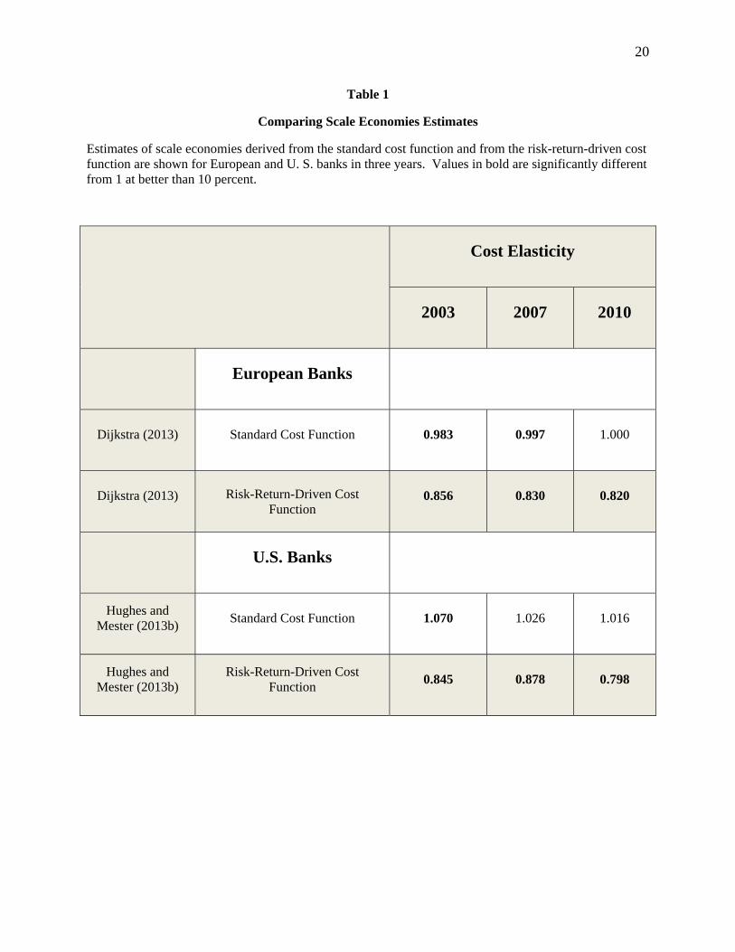
Do big banks experience overall scale economies?

The estimation of the risk-return-driven cost function in equation (3) reveals the scale

economies that elude the standard cost function. Dijkstra (2013) estimates both the standard cost

function and the risk-return-driven cost function for European banks in 2003, 2007, and 2010.

Table 1 reports the cost elasticities he obtains. For the standard cost function, the cost elasticity

is either 1 or very close to 1 for the three years – essentially constant returns to scale. By

controlling for the investment strategy, the risk-return-driven cost function yields estimates of

the cost elasticity that imply a 10 percent increase in outputs is associated with an 8.56 percent

increase in cost in 2003, an 8.30 percent increase in 2007, and an 8.20 percent increase in 2010 –

evidence of large scale economies that elude the standard cost function.

Hughes and Mester (2013b) find similar results for the same three years for top-tier U.S.

bank holding companies. The standard cost function yields cost elasticities that imply either

scale diseconomies or constant returns to scale: in 2003, a 10 percent increase in outputs results

in a 10.7 percent increase in cost; in 2007 and 2010, the cost elasticities are not statistically

different from one. In contrast, after controlling for the investment strategy, the risk-return-

driven cost function provides evidence of substantial cost economies: a 10 percent increase in

outputs implies an 8.45 percent increase in cost in 2003, an 8.78 percent increase in 2007, and a

7.98 percent increase in 2010.

13

[INSERT TABLE 2 HERE]

Not only do Hughes and Mester (2013b) find evidence of substantial scale economies for

all three years, they also find that the largest banks experience the largest scale economies. In

Table 2, the estimates of cost elasticities are broken down by size groups. Consider a

comparison of the mean cost elasticities of banks in the range of $2 - $10 billion in assets to

those of banks whose assets exceed $100 billion. For a 10 percent increase in outputs, in 2003

cost increases by 8.34 percent for the smaller banks and 7.37 percent for the very large banks; in

2007, 8.70 percent for smaller banks and 7.49 percent for the largest; and in 2010, 7.54 percent

for the smaller banks and 7.00 percent for the largest.9

Are the scale economies found for the largest financial institutions generated by a more efficient production technology or by cost-of-funds subsidies because of being perceived as too big to fail? Hughes and Mester (2013b) conduct tests to determine whether technology or cost-of-

funds subsidies due to too-big-to-fail account for the estimated scale economies of the largest

financial institutions. Using the 2007 data on U.S. banks, they re-estimate the cost function after

dropping banks larger than $100 billion in assets, the so-called too-big-to-fail banks.10 They then

calculate the cost elasticity for the largest banks whose assets exceed $100 billion out-of-sample

based on the fitted cost function. Compared to the baseline cost elasticity of 0.749 for these

banks reported in Table 2, they obtain a cost elasticity of 0.742. If the largest institutions benefit

from a lower cost of funds because of being perceived as too big to fail, their elimination from

the estimation and the out-of-sample calculation of nearly the same value of cost elasticity 9 The estimate of a mean cost elasticity of 0.700 in 2010 for banks whose assets exceed $100 billion is consistent with approximately $14 - $19 billion in cost synergies at $2.4 trillion in consolidated assets, the size of JPMorgan Chase at the time of the Goldman report on breaking up JP Morgan Chase and the response by CFO Marianne Lake that JPMorgan Chase has approximately $18 billion in cost synergies. 10 See Brewer and Jagtiani (2009) for a discussion of the definition of the too-big-to-fail classification.

14

provides compelling evidence that the study’s estimated scale economies at the largest

institutions are not being driven by the perception of being too big to fail.

The authors also performed an additional test to see whether the estimate of scale

economies at banks whose assets exceed $100 billion is being driven by a cost-of-funding

advantage from being perceived as too big to fail. They recalculated estimated cost elasticities

for these banks, replacing their actual cost-of-funds with the median cost-of-funds for banks in

the sample with $100 billion or less in assets. The mean cost elasticity for the too-big-to-fail

banks with these pseudo-prices is 0.743 compared to the baseline 0.749. This is suggestive that

it is production technology, not perceptions about being too-big-to-fail, that generates the scale

economies of the largest financial institutions.11

Thus, while there may be a funding cost advantage among the largest banks (perhaps

because they are perceived as being too-big-to-fail), the risk-return-driven cost function controls

for this funding advantage when computing scale economies, and there is no evidence that a

funding cost advantage influences the estimates of scale economies.

11 Davies and Tracey (2014) estimate a standard cost function for European banks and obtain significant scale economies. They test the robustness of this result by replacing the interest rate paid on borrowed funds with the interest rate implied by Moody’s rating, assuming no government or outside assistance in the case of financial distress. While using the actual observed price of borrowed funds yields evidence of scale economies, these economies disappear when the pseudo-price is used in the estimation. They assume that this difference in measured scale economies is due to a too-big-to-fail subsidy. Hughes and Mester (2013b) point out some weaknesses of the Davies and Tracey (2014) approach. While Hughes and Mester use a pseudo-price strategy, they substitute the pseudo-prices into the equation for the cost elasticity derived from the cost function estimated with the observed prices. In contrast, Davies and Tracey re-estimate the cost function using the pseudo-prices and the total cost and input expenditures that correspond to the original observed prices. Their model assumes that cost is minimized with respect to the pseudo-prices, but the total costs and cost shares belong to the observed prices, not the pseudo-prices. Since the pseudo-prices do not give rise to the total costs used in the re-estimation, the evidence obtained from the re-estimation is hard to interpret and cannot be considered evidence that the too-big-to-fail policy generates the scale economies.

15

How would restrictions on the size of the largest financial institutions affect their global competitiveness?

Tarullo (2011) describes the trade-off between systemic risk and efficiency: “An

additional concern would arise if some countries made the trade-off by limiting the size or

configuration of their financial firms for systemic risk reasons at the cost of realizing genuine

economies of scope or scale, while other countries did not. In this case, firms from the first

group of countries might well be at a competitive disadvantage in the provision of certain cross-

border activities.”

Wheelock and Wilson (2012) compare the cost of the 4 largest institutions in 2009

($1.244 - $2.225 trillion) with a number of $1 trillion institutions equaling the total assets of the

four largest institutions. The combined cost of the scaled-down institutions is 9 percent higher.

Hughes and Mester (2013b) compare the cost of the 17 largest institutions whose assets

exceeded $100 billion in 2007 with these institutions scaled back to half their size with the same

product mix. They increase the number of smaller institutions so that the combined assets equal

the assets of the 17 largest institutions. The cost of the scaled-down institutions is 23 percent

higher.

Proposals to limit the size of banks or to break up existing large institutions to reduce

systemic risk face the problem that economic incentives reward scale and scope. Smaller

institutions will produce at higher average cost and will likely not be able to provide the variety

of financial products and services that characterize larger institutions. Because such size

restrictions would work against market forces, they would create incentives for companies to

avoid them. An obvious strategy entails operating outside the more regulated sector where there

is no assurance that new sources of systemic risk will not develop. Thus, the incentive to escape

regulatory restrictions on the size and configuration of financial institutions would require

16

intensive research and monitoring, roles currently assigned in the U.S. to the Office of Financial

Research and the Financial Stability Oversight Council.

Conclusions

Scale economies are hard to detect empirically because costly endogenous risk-taking

interacts with the production technology, which tends to obscure them. Empirical results based

on models that account for endogenous risk-taking indicate that the largest financial institutions

experience the largest scale economies and that technological advantages, such as diversification

and the spreading of information costs and other costs that do not increase proportionately with

size, rather than safety-net subsidies appear to generate the scale economies.

It is very important to note that the literature does not indicate whether these benefits of

larger size outweigh the potential costs in terms of the systemic risk that large scale may impose

on the financial system. More research is needed to calibrate efficiency benefits against potential

system risks posted by large, complex institutions. However, the finding of significant scale

economies does suggest that if public policy considerations imply that society would be better

off with smaller financial institutions, restrictions that limit the size of financial institutions, if

effective, may put large banks at a competitive disadvantage in global markets where

competitors are not similarly constrained. Moreover, size restrictions may not be effective since

they work against market forces and create incentives for firms to avoid them. Avoiding the

restrictions could thereby push risk-taking outside of the more regulated financial sector without

necessarily reducing systemic risk. These factors need to be considered when evaluating policies

concerning financial institution scale.

17

References Bair, Sheila, January 18, 2012, “Why it’s time to break up the ‘too big to fail’ banks,” Fortune. Becalli, E., Anolli, M., Borello, G., 2015, “Are European banks too big? Evidence on economies of scale,” Journal of Banking and Finance, Vol. 58, pp. 232-246. Berger, A.N., Mester, L.J., 1997, “Inside the black box: What explains differences in the efficiencies of financial institutions?” Journal of Banking and Finance, Vol. 21, pp. 895-947. Bossone, B., Lee, J.-K., 2004, “In finance, size matters: The ‘systemic scale economies’ hypothesis,” IMF Staff Papers, Vol. 51:1. Brewer, E., Jagtiani, J., 2009, “How much did banks pay to become too-big-to-fail and to become systemically important?” Federal Reserve Bank of Philadelphia Working Paper No. 09-34. Davies, R., Tracey, B., 2014, “Too big to be efficient? The impact of too-big-to-fail factors on scale economies for banks,” Journal of Money, Credit, and Banking, Vol. 46, pp. 219-253. Deaton, A., Muellbauer, J., 1980, “An almost ideal demand system,” American Economic Review, Vol. 70, pp. 312-326. Demsetz, R. S. and Strahan, P. E., 1997, “Diversification, size, and risk at bank holding companies,” Journal of Money, Credit, and Banking, Vol. 29, pp. 300–313. Dijkstra, M., 2013, “Economies of scale and scope in the European banking sector 2002-2011,” Amsterdam Center for Law & Economics Working Paper No. 2013-11. Feng, G., Serletis, A., 2010, “Efficiency, technical change, and returns to scale in large US banks: Panel data evidence from an output distance function satisfying theoretical regularity,” Journal of Banking and Finance, Vol. 34, pp. 127-138. Fisher, R. and Rosenblum, H., April 4, 2012, “How huge banks threaten the economy,” The Wall Street Journal. Greenspan, A., 2010, “The crisis,” Brookings Papers on Economic Activity, pp. 201-246. Hughes, J.P., Lang, W., Mester, L.J., Moon C.-G., 1996, “Efficient banking under interstate branching,” Journal of Money, Credit, and Banking, Vol. 28, pp. 1045-1071. Hughes, J.P., Lang, W., Mester, L.J., Moon C.-G., 2000, “Recovering risky technologies using the almost ideal demand system: An application to U.S. banking,” Journal of Financial Services Research, Vol. 18, pp. 5-27.

18

Hughes, J.P., Mester, L.J., 1998, “Bank capitalization and cost: Evidence of scale economies in risk management and signaling,” Review of Economics and Statistics, Vol. 80, pp. 314-325. Hughes, J.P. and Mester, L.J., 2013a, “A primer on market discipline and governance of financial institutions for those in a state of shocked disbelief,” Chapter 2 in Efficiency and Productivity Growth: Modelling in the Financial Services Industry, ed. Pasiouras, F., John Wiley and Sons: West Sussex, U.K., pp. 19-47. Hughes, J.P. and Mester, L.J., 2013b, “Who said large banks don’t experience scale economies? Evidence from a risk-return-driven cost function,” Journal of Financial Intermediation, Vol. 22, pp. 559-585. Hughes, J.P., Mester, L.J. and Moon, C.-G., 2001, “Are scale economies in banking elusive or illusive? Evidence obtained by incorporating capital structure and risk-taking into models of bank production,” Journal of Banking and Finance, Vol. 25, pp. 2169-2208. Kovner, A., Vickery, J., and Zhou, L., 2014, “Do big banks have lower operating costs?” Federal Reserve Bank of New York Economic Policy Review, Dec., pp. 1-27. Marcus, A.J., 1984, “Deregulation and bank financial policy,” Journal of Banking and Finance, Vol. 8, pp. 557-565. Popper, N., February 24, 2015, “JPMorgan Chase insists it’s worth more as one than in pieces,” The New York Times. Purcell, P., June 25, 2012, “Shareholders can cure too big to fail,” Wall Street Journal. Ramsden, R., Fitzgerald, C., Parls, D., and Senet, K., January 5, 2015, “New capital rules reignite the JPM breakup debate,” Goldman Sachs Equity Research, United States: Banks. Tarullo, Daniel K., 2011, “Industrial organization and systemic risk: An agenda for further research,” Conference on the Regulation of Systemic Risk, Federal Reserve Board, Washington, D.C. Wheelock, D., Wilson, P., 2012, “Do large banks have lower costs? New estimates of returns to scale for US banks,” Journal of Money, Credit, and Banking, Vol. 44, pp. 171-99. Wheelock, D. C., Wilson, P. W., 2015, “The evolution of scale economies in U.S. banking,” Federal Reserve Bank of St. Louis, Working Paper 2015-021A.

19

Expected Return

0 RiskB RiskA= RiskC RiskD Risk

Figure 1

Scale Economies as a Function of Risk-Expected Return Trade-Off From Hughes and Mester (2013b)

ERB

ERC

ERD

ERA A

B

C

D smaller output

larger output

20

Table 1

Comparing Scale Economies Estimates

Estimates of scale economies derived from the standard cost function and from the risk-return-driven cost function are shown for European and U. S. banks in three years. Values in bold are significantly different from 1 at better than 10 percent.

Cost Elasticity

2003 2007 2010

European Banks

Dijkstra (2013) Standard Cost Function 0.983 0.997 1.000

Dijkstra (2013) Risk-Return-Driven Cost Function

0.856 0.830 0.820

U.S. Banks

Hughes and Mester (2013b)

Standard Cost Function 1.070 1.026 1.016

Hughes and Mester (2013b)

Risk-Return-Driven Cost Function

0.845 0.878 0.798

21

Table 2

Cost Elasticities Estimated from the Risk-Return-Driven Cost Function From Hughes and Mester (2013b)

Estimates of scale economies derived from the risk-return-driven cost function are shown for U. S. banks in three years. Values in bold are significantly different from 1 at better than 10 percent.

Cost Elasticity

Consolidated Assets 2003 2007 2010

< $0.8 billion 0.855 0.891 0.815

$0.8 - $2 billion 0.833 0.882 0.814

$2 - $10 billion 0.834 0.870 0.754

$10 - $50 billion 0.731 0.846 0.763

$50 - $100 billion 0.711 0.812 0.701

> $100 billion 0.737 0.749 0.700