Short title: The Fundamental Law of Road Congestion

The Fundamental Law of Road Congestion:Evidence from US cities

By GILLES DURANTON AND MATTHEW A. TURNER*

We investigate the effect of lane kilometers of roads on vehicle-kilometers traveled (VKT) in US cities.

VKT increases proportionately to roadway lane kilometers for interstate highways and probably

slightly less rapidly for other types of roads. The sources for this extra VKT are increases in driving

by current residents, increases in commercial traffic, and migration. Increasing lane kilometers for

one type of road diverts little traffic from other types of road. We find no evidence that the provision

of public transportation affects VKT. We conclude that increased provision of roads or public transit

is unlikely to relieve congestion. (JEL R41, L91)

We investigate the effect of lane kilometers of roads on vehicle-kilometers traveled (VKT) for different

types of roads in the United States (US). For interstate highways in metropolitan areas we find that VKT

increases one for one with interstate highways, confirming the ‘fundamental law of highway congestion’

suggested by Anthony Downs (1962; 1992). We also uncover suggestive evidence that this law may extend

beyond interstate highways to a broad class of major urban roads, a ‘fundamental law of road congestion’.

These results suggest that increased provision of interstate highways and major urban roads is unlikely to

relieve congestion of these roads.

Our investigation is of interest for three reasons. First, an average American household spent 161

person-minutes per day in a passenger vehicle in 2001. These minutes allowed 134 person-km of auto

*Duranton: Department of Economics, University of Toronto, 150 Saint George Street, Toronto, Ontario M5S 3G7,

Canada (e-mail: gilles.duranton@utoronto.ca; website: http://individual.utoronto.ca/gilles/default.html).

Also affiliated with the Centre for Economic Policy Research, the Rimini Centre for Economic Analysis, and the Centre

for Economic Performance at the London School of Economics; Turner: Department of Economics, University of

Toronto, 150 Saint George Street, Toronto, Ontario M5S 3G7, Canada (e-mail: mturner@chass.utoronto.ca; website:

http://www.economics.utoronto.ca/mturner/index.htm).). We thank Richard Arnott, Severin Borenstein, Klaus

Desmet, Jan Brueckner, Victor Couture, Edward Glaeser, Steve Kohlhagen, Andreas Kopp, David Levinson, Guy

Michaels, Se-Il Mun, Ken Small, two anonymous referees who clearly went beyond the call of duty, and seminar and

conference participants for comments and suggestions. Thanks also to Byron Moldofsky for assistance with GIS and data

processing and Magda Biesiada for excellent research assistance. Financial support from the Canadian Social Science

and Humanities Research Council and the Paris School of Economics is gratefully acknowledged by both authors.

1

travel at an average speed of 44 km/h. Multiplying by the number of households in the US and any

reasonable dollar value of time, we see that the US allocated considerable resources to passenger vehicle

travel. That Americans rank commuting among their least enjoyable activities (Alan B. Krueger et al., 2009)

buttresses our suspicion that the costs of congestion are large. To the extent that travel resources could

have been better allocated, understanding congestion and the effect of potential policy interventions is an

important economic problem.

Second, since the costs of congestion and of transportation infrastructure are both large, transportation

policy should be based on the careful analysis of high quality data, not on the claims of advocacy groups.

Unfortunately, there is currently little empirical basis for accepting or rejecting the claims by the American

Road and Transportation Builders Association that “adding highway capacity is key to helping to reduce traffic

congestion”, or of the American Public Transit Association that without new investment in public transit,

highways will become so congested that they “will no longer work”.1 Our results do not support either of

these claims.

Third, with the increasing certainty of global warming comes the need to manage carbon emissions.

According to the US Bureau of Transportation Statistics (2007, chapter 4) the road transportation sector

accounts for about a third of US carbon emissions from energy use. Understanding the implications for

VKT of changes to transportation infrastructure is immediately relevant to this policy problem.

Ours is not the first attempt to measure the effect of the supply of roads on traffic. Following Roy E.

Jorgensen (1947), a large literature estimates new traffic for particular facilities after their opening or after a

capacity expansion (see Phil B. Goodwin, 1996; Robert Cervero, 2002, for reviews).2 However studies of a

particular road provide little basis for assessing the impact that changes in infrastructure have on traffic in

the city at large, a question that is probably more relevant to transportation policy. As Cervero’s (2002)

review shows, few studies take an approach similar to ours and assess the effect of road provision on traffic

over entire areas. These studies generally find a positive elasticity of VKT to the supply of roads, although

their estimates of this elasticity vary widely. We improve on this literature in three respects.

First, we use more and more comprehensive data. To begin, we take average annual daily traffic (AADT)

and a description of the road network from the US Highway Performance and Monitoring System (HPMS)

for 1983, 1993, and 2003. We add a description of individual and household travel behavior taken from the

1995 Nationwide Personal Transportation Survey and 2001 National Household Travel Survey (which we

1The quote from the APTA is at www.apta.com/government_affairs/aptatest/documents/testimony060921.pdf.

The quote from the ARTBA is harder to find and occurs in an undated flyer which is no longer available on their website,

http://www.artba.org/.2While Jorgensen (1947) is our first modern source, the analysis of the effects of new facilities such as bridges and

their tariffs on flows of vehicles follows a much older tradition, dating back to Jules E.J. Dupuit (1844).

2

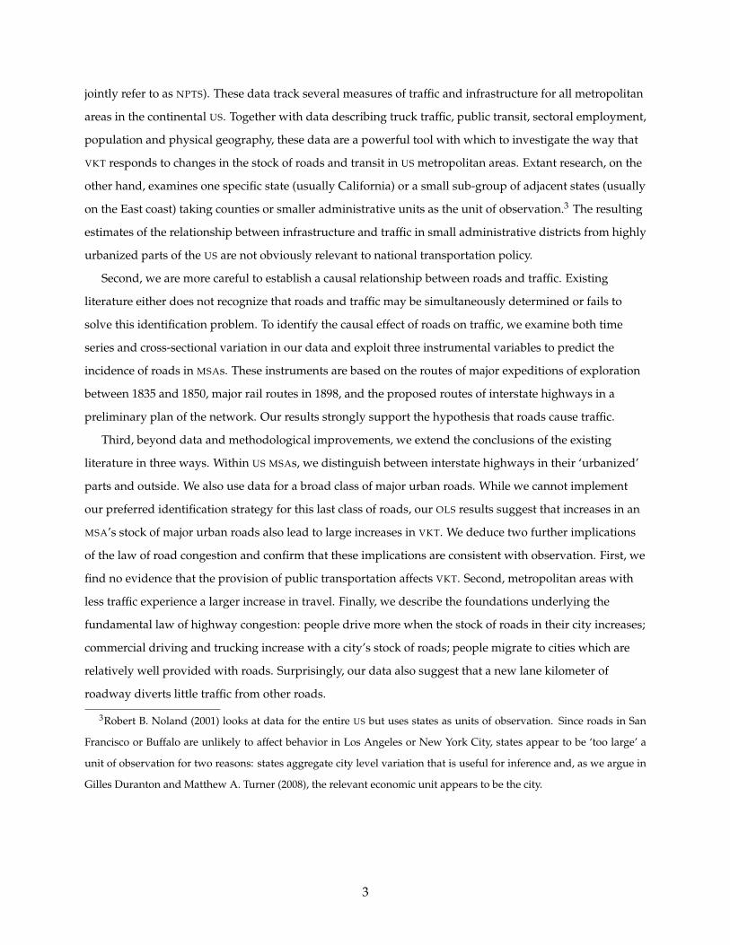
jointly refer to as NPTS). These data track several measures of traffic and infrastructure for all metropolitan

areas in the continental US. Together with data describing truck traffic, public transit, sectoral employment,

population and physical geography, these data are a powerful tool with which to investigate the way that

VKT responds to changes in the stock of roads and transit in US metropolitan areas. Extant research, on the

other hand, examines one specific state (usually California) or a small sub-group of adjacent states (usually

on the East coast) taking counties or smaller administrative units as the unit of observation.3 The resulting

estimates of the relationship between infrastructure and traffic in small administrative districts from highly

urbanized parts of the US are not obviously relevant to national transportation policy.

Second, we are more careful to establish a causal relationship between roads and traffic. Existing

literature either does not recognize that roads and traffic may be simultaneously determined or fails to

solve this identification problem. To identify the causal effect of roads on traffic, we examine both time

series and cross-sectional variation in our data and exploit three instrumental variables to predict the

incidence of roads in MSAs. These instruments are based on the routes of major expeditions of exploration

between 1835 and 1850, major rail routes in 1898, and the proposed routes of interstate highways in a

preliminary plan of the network. Our results strongly support the hypothesis that roads cause traffic.

Third, beyond data and methodological improvements, we extend the conclusions of the existing

literature in three ways. Within US MSAs, we distinguish between interstate highways in their ‘urbanized’

parts and outside. We also use data for a broad class of major urban roads. While we cannot implement

our preferred identification strategy for this last class of roads, our OLS results suggest that increases in an

MSA’s stock of major urban roads also lead to large increases in VKT. We deduce two further implications

of the law of road congestion and confirm that these implications are consistent with observation. First, we

find no evidence that the provision of public transportation affects VKT. Second, metropolitan areas with

less traffic experience a larger increase in travel. Finally, we describe the foundations underlying the

fundamental law of highway congestion: people drive more when the stock of roads in their city increases;

commercial driving and trucking increase with a city’s stock of roads; people migrate to cities which are

relatively well provided with roads. Surprisingly, our data also suggest that a new lane kilometer of

roadway diverts little traffic from other roads.

3Robert B. Noland (2001) looks at data for the entire US but uses states as units of observation. Since roads in San

Francisco or Buffalo are unlikely to affect behavior in Los Angeles or New York City, states appear to be ‘too large’ a

unit of observation for two reasons: states aggregate city level variation that is useful for inference and, as we argue in

Gilles Duranton and Matthew A. Turner (2008), the relevant economic unit appears to be the city.

3

0

P

VKTQ∗ Q∗′

P(Q)

AC(R)

AC(R′)

1

FIGURE 1—SUPPLY AND DEMAND FOR ROAD TRAFFIC.

I. Roads and traffic: a simple framework

To motivate our econometric strategy consider a simple model of equilibrium VKT. To begin, let R denote

lane kilometers of roads in a city, let Q denote VKT, and let P(Q) be the inverse demand for VKT. The

downward sloping line in figure 1 represents an inverse VKT demand curve for a particular city.

Let C(R,Q) be the total variable cost of VKT, Q, given roads, R. In equilibrium all drivers face the same

average cost of travel. Holding lane kilometers constant at R, the average cost of driving increases with

VKT. Hence, the average cost curve for VKT is upward sloping. This feature is well documented in the

transportation literature (Kenneth A. Small and Erik T. Verhoef, 2007). The leftmost upward sloping curve

in figure 1 represents the supply curve AC(R) associated with roads R.

Equilibrium VKT, Q∗(R) is characterized by

(1) P(Q∗) =C(R,Q∗)

Q∗.

That is, willingness to pay equals average cost.

Increasing the supply of road lane kilometers from R to R′ reduces the average cost of driving for any

level of VKT.4 It thus shifts the average cost curve to the right. With R lane kilometers of roads in the city,

the demand curve intersects with the supply curve at Q∗, the equilibrium VKT. With R′

lane kilometers of

road, the corresponding equilibrium implies a VKT of Q′∗.

4There are pathological examples where increases in the extent of a road network can reduce its capacity, in particular

the ‘Braess paradox’ described in Small and Verhoef (2007). We ignore such pathological examples here.

4

We would like to learn the effect of an increase in the stock of roads on driving in cities. That is, we

would like to learn about the function Q∗(R) defined implicitly by equation (1). Indexing cities by i and

years by t, our problem may be stated as one of estimating,

(2) ln(Qit) = A0 + ρQR ln(Rit) + A1Xit + εit,

where X denotes a vector of observed city characteristics and ε describes unobserved contributors to

driving. We are interested in the coefficient of R, the road elasticity of VKT, ρQR ≡ ∂ ln Q/∂ ln R.

With data describing driving and the stock of roads in a set of cities, we can estimate equation (2) with

OLS to obtain consistent estimates of ρQR , provided that cov(R,ε|X) = 0. In practice, we hope that roads will

be assigned to growing cities and fear that they are assigned to prop-up declining cities. In either case, the

required orthogonality condition fails. Thus, we are concerned that estimating equation (2) will not lead to

the true value of ρQR .

As a next step, we partition ε into permanent and time varying components, and write

(3) ln(Qit) = A0 + ρQR ln(Rit) + A1Xit + δi + ηit.

With data describing a panel of cities, we can estimate this equation using city fixed effects to remove all

time invariant city effects. This leads to consistent estimates of ρQR , provided that cov(R,η|X,δ) = 0. We also

estimate the first difference equation,

(4) ∆ ln(Qit) = ρQR ∆ ln(Rit) + A1∆Xit + ∆ηit,

where ∆ is the first difference operator. Since all time invariant factors drop out of the first difference

equation, we are left with essentially the same orthogonality requirement as for equation (3).5 If, in

equation (4), we include city characteristics in level and initial VKT as control variables, then we account for

the possibility that these initial conditions may determine traffic growth and be correlated with changes in

roadway.

To our knowledge, there is no study of a comprehensive set of metropolitan areas in the literature. The

extant literature, however, has estimated variants of equations (2), (3), and (4) on a small samples of

counties or metropolitan areas. While the early literature on induced demand at the area level (e.g. Frank S.

Koppelman, 1972) only ran simple OLS regressions in the spirit of equation (2), second generation work on

the issue typically explored a variety of specifications with fixed effects and, sometimes, a complex lag

structure. For instance, Mark Hansen et al. (1993) and Hansen and Yuanlin Huang (1997) use panels of

urban counties and MSAs in California while Noland (2001) uses a panel of US states. All find a positive

5In fact, the two estimates have subtly different properties, see Jeffrey M. Wooldridge (2001, chapter 4).

5

association between VKT and lane kilometers of roadway, with estimated elasticities generally ranging

between 0.3 and 0.7.

While equations (3) and (4) improve upon equation (2), we are concerned that roads will be assigned to

cities in response to a contemporaneous shock to the city’s traffic. To deal with this identification issue, we

model the assignment of roads to cities explicitly. This leads to a two equation model, one to predict the

assignment of roads to cities, the other to predict the effect of roads on traffic,

ln(Rit) = B0 + B1Xit + B2Zit + µit

ln(Qit) = A0 + ρQR̂ln(Rit) + A1Xit + εit,

(5)

where ̂ln(Rit) is predicted lane kilometers of roadway as estimated in the first stage. We can obtain

consistent estimates of ρQR provided that we are able to find instruments to satisfy cov(Z,R|X) 6= 0 and

cov(Z,ε|X) = 0.

The possible simultaneous determination of VKT and lane kilometers is recognized by several authors.

To instrument for lane kilometers of highways Cervero and Hansen (2002) use about 20 instruments

describing politics and physical geography. This approach is subject to the problems associated with the

use of a large number of instruments. Moreover, we expect the physical geography of cities, climate in

particular, to affect the demand for travel directly in addition to affecting the supply of roads. This violates

the condition cov(Z,ε|X) = 0 and invalidates the instruments. Noland and William A. Cowart (2000) use

land area and population density as instruments for lane kilometers of roads. Again, we expect population

density to be a determinant of the demand for travel as much as a determinant of the supply of roads.

Lewis M. Fulton et al. (2000) instrument growth in lane kilometers of highways by short lags of the same

variables in a first difference specification. The exclusion restriction then requires that past changes in road

supply be uncorrelated with contemporaneous changes in demand. Since changes in road supply are

serially correlated (and they need to be so for the instrument to have any predictive power), the exclusion

restriction is unlikely to hold when new roads are supplied as a result of VKT demand shocks. We postpone

a discussion of our own choice of instruments.

Each of the approaches described above relies on different variation in the data to estimate ρQR .

Equation (2) relies on cross-sectional variation, while equations (3) and (4) use only time series variation.

Equation (5) exploits the instrumental variables we describe later. Should all three methods arrive at the

same estimate of ρQR , then all are correct, or all are incorrect and an improbable relationship exists between

the various errors and instrumental variables.

We now turn to a description of our data and estimates of ρQR based on the estimating equations

presented in this section.

6

II. Data and estimation

We take the (Consolidated) Metropolitan Statistical Area (MSA) drawn to 1999 boundaries as our unit of

observation. Since each MSA aggregates one or more counties, MSA boundaries often encompass much

land that is not ‘urban’ in the common sense of the word. However, MSAs are generally organized around

one or more ‘urbanized areas’ which make up the core(s) of the MSA and typically occupy only a fraction of

an MSA’s land area. By using data collected at the level of ‘urbanized areas’ we can distinguish more from

less densely developed parts of each metropolitan area.

To measure each MSA’s stock of interstate highways and traffic we use the US Highway Performance

and Monitoring System (HPMS) ‘Universe’ and ‘Sample’ data for 1983, 1993, and 2003.6 The data appendix

provides a more detailed description of the HPMS. The Federal Highway Administration in the US

Department of Transportation (DOT) collects these data, which are used by the federal government for

planning purposes and to apportion federal highway money. For each year, for the entire universe of the

interstate highway system within their boundaries states must report the length, number of lanes, and the

number of vehicles per lane per day passing any point. This last quantity is referred to as the average

annual daily traffic (AADT). We use a county identifier to match every segment of interstate highway to an

MSA. We then calculate lane kilometers, VKT, and AADT per lane km for interstate highways within each

MSA.

In the Sample data states report the same information (and more) for every segment of interstate

highway within urbanized areas. By merging the Sample with the Universe data we distinguish urban

from non urban interstates within MSAs.

The Sample data also report information about a sample of other roads within urbanized areas. This

sample is intended to represent all major roads in urbanized areas within the state. From the sample data

we calculate road length, location, AADT and share of truck traffic for all major roads in the urbanized area.

The HPMS sample data also assigns each segment to one of six functional classes, described in DOT (1989).

One of these classes is ‘interstate highway’. We group four of the remaining five classes; ‘collector’, ‘minor

arterial’, ‘principal arterial’, and ‘other highway’ into a measure of major urban roads, omitting the last

class, ‘local roads’.7 Our definition of ‘major urban road’ thus includes all non local roads that are not

6The HPMS is available annually. We focus on 1983, 1993 and 2003 because these dates are close to census years and

to the years for which we have data on public transportation. In addition, we sometimes make use of the 1995 and 2001

HPMS.7Loosely, a ‘local road’ is one that primarily provides access to land adjacent to the road and every other class of road

serves to connect local roads. The HPMS does not require states to report data on local roads, although some local roads

appear in the data.

7

TABLE 1—SUMMARY STATISTICS FOR OUR MAIN HPMS AND PUBLIC TRANSPORTATION VARIABLES

Year: 1983 1993 2003

Mean daily VKT (IH,’000 km) 7,777 11,905 15,961(16,624) (24,251) (31,579)

Mean AADT (IH) 4,832 7,174 9,361(2,726) (3,413) (4,092)

Mean lane km (IH) 1,140 1,208 1,280(1,650) (1,729) (1,858)

Mean lane km (IH, per 10,000 population) 26.7 24.3 22.1(26.9) (20.9) (16.4)

Mean daily VKT (MRU,’000 km) 14,553 22,450 31,242(36,303) (49,132) (70,692)

Mean AADT (MRU) 3,146 3,646 3,934(847) (947) (1,059)

Mean lane km (MRU) 3,885 5,071 6471(7,926) (9,119) (12,426)

Mean VKT share urbanized (IHU/IH) 0.38 0.44 0.48Mean lane km share urbanized (IHU/IH) 0.29 0.36 0.40Mean share truck AADT (IH) 0.11 0.12 0.13Peak service large buses per 10,000 population 1.20 1.09 1.34

(1.02) (0.98) (0.98)Peak service large buses 169 165 217

(563) (562) (742)Number MSAs 228 228 228Mean MSA population 753,726 834,290 950,054

Notes: Cross MSA means and standard deviations between brackets. IH denotes interstate highways for the entire MSA.IHU denotes interstate highways for the urbanized areas within an MSA. MRU denotes major roads for the urbanizedareas within an MSA.

interstate highways. Within urbanized areas, interstates represent about 1.5 percent of all road kilometers

and 24 percent of VKT while major urban roads represent 27 percent of road kilometers and another 62

percent of VKT (DOT, 2005a). The data appendix provides more detail.

Table 1 presents MSA averages of AADT for the 228 MSAs with non zero interstate milage in 1983, 1993,

and 2003. These data show that AADT, the number of vehicles passing any point on an average lane of

interstate highway, increased from 4,832 in 1983 to 9,361 in 2003. Thus, at the end of our study period, an

average lane of interstate highway carries almost twice as much traffic as at the beginning. We also find

that lane kilometers of interstate highways increase by about 6 percent between 1983 and 1993 and

between 1993 and 2003. Together, the increase in lane kilometers and the increase in AADT imply that

interstate VKT in an average MSA more than doubled over our twenty year study period.

Table 1 also presents descriptive statistics for major urban roads. Major roads represent between three

and five times as many lane kilometers as interstate highways but only twice as much VKT. Note that

urbanized area boundaries, unlike MSA boundaries, are not constant over our three cross-sections, so the

8

dramatic increase in urbanized area VKT and lane kilometers over our study period may partly reflect

increases in the extent of urbanized areas.

A. Cross-sectional estimates of the roadway elasticity of VKT

We now turn to estimating the elasticity of MSA VKT to lane kilometers for each of the following categories

of roads and travel: All MSA interstates (IH), urbanized MSA interstates (IHU), non urban MSA interstates

(IHNU), and major urban roads (MRU). Table 2 presents estimates of this elasticity for four specifications of

the cross-sectional equation (2) for each type of road in 1983, 1993, and 2003.

In panel A of this table, the dependent variable is MSA interstate VKT. Columns 1 to 4 consider the 1983

cross-section. In the first column we include only our variable of interest, the log of lane kilometers of road,

and a constant. In the second we add MSA population. In the third, we add nine census division dummy

variables along with five measures of physical geography: elevation range within the MSA, the ruggedness

of terrain in the MSA, two measures of climate, and a measure of how dispersed is development in the MSA.

Details about these variables are available in the data appendix. In column 4 we also add socio-economic

controls; share of population with at least some college education, log mean income, share poor, share of

manufacturing employment, and an index of segregation. We also add decennial population variables

from 1920-1980 to control for the long-run growth of MSAs. Because Past populations and socio-economic

variables are likely to correlate with unobserved attributes of MSAs that determine the demand for driving,

regressions including these variables are useful robustness checks. Columns 5 to 8 replicate these

regressions for 1993, while columns 9-12 are for 2003.

Depending on the decade, the elasticity of MSA interstate highway VKT with respect to lane kilometers

is between 1.23 and 1.25 when estimated without controls, ranges between 0.71 and 0.94 in specifications

with controls, and is estimated precisely in each specification. While some estimates are statistically

different from one, all are positive and greater than 0.71.

Turning to the other explanatory variables, we also note that the elasticity of MSA interstate highway

VKT with respect to population is much less than one in all specifications. This will persist in nearly all of

our estimations and suggests that people in larger cities drive much less, per capita, than they do in

smaller cities. We consider the possible endogeneity of this variable below. We also note that VKT is higher

in MSAs with mild weather, neither cold nor hot. For the other measures of geography, including the extent

to which development is scattered or compact, as measured by the variable ‘sprawl’, we do not find a

robust association with MSA interstate highway VKT.

Panel B of table 2 is similar to panel A, but the dependent variable and the measure of roads are based

on urban interstates. The estimations in panel B suggest that the urban interstate VKT elasticity of urban

9

TABLE 2—VKT AS A FUNCTION OF LANE KILOMETERS, OLS BY DECADE.

[1] [2] [3] [4] [5] [6] [7] [8] [9] [10] [11] [12]Year: 1983 1983 1983 1983 1993 1993 1993 1993 2003 2003 2003 2003

Panel A. Dependent variable: ln VKT for Interstate Highways, entire MSAs

ln(IH lane km) 1.24a 0.92a 0.94a 0.92a 1.25a 0.73a 0.76a 0.77a 1.23a 0.71a 0.75a 0.76a

(0.04) (0.06) (0.06) (0.05) (0.02) (0.05) (0.04) (0.04) (0.02) (0.05) (0.04) (0.04)ln(population) 0.43a 0.42a 1.01a 0.54a 0.51a 0.46c 0.53a 0.49a 0.39

(0.04) (0.05) (0.37) (0.04) (0.04) (0.25) (0.04) (0.04) (0.35)Elevation range -0.057 -0.076 -0.027 -0.038 -0.026 -0.030

(0.060) (0.054) (0.056) (0.054) (0.053) (0.048)Ruggedness 6.81c 5.29 5.86c 3.90 5.72c 3.46

(3.46) (3.24) (3.00) (3.00) (3.06) (3.11)Heating degree days -0.014a -0.015a -0.012a -0.013a -0.011a -0.013a

(0.004) (0.01) (0.003) (0.004) (0.003) (0.004)

Cooling degree days -0.019c -0.027b -0.019a -0.022b -0.019b -0.020b

(0.010) (0.012) (0.007) (0.009) (0.007) (0.009)Sprawl 0.0059c 0.0061c 0.0033 0.0019 0.0021 0.0016

(0.0031) (0.0036) (0.0028) (0.0029) (0.0027) (0.0027)Census divisions Y Y Y Y Y YPast populations Y Y YSocio-econ. charac. Y Y Y

R2 0.86 0.93 0.94 0.95 0.87 0.94 0.95 0.96 0.88 0.94 0.96 0.96

Panel B. Dependent variable: ln VKT for Interstate Highways, urbanized areas within MSAs

ln(IHU lane km) 1.26a 1.04a 1.05a 1.06a 1.23a 0.95a 0.97a 1.00a 1.20a 0.92a 0.94a 0.97a

(0.02) (0.03) (0.03) (0.03) (0.02) (0.03) (0.03) (0.04) (0.02) (0.03) (0.03) (0.04)

Panel C. Dependent variable: ln VKT for Major Roads, urbanized areas within MSAs

ln(MRU lane km) 1.08a 0.90a 0.89a 0.88a 1.13a 0.72a 0.78a 0.80a 1.14a 0.66a 0.67a 0.70a

(0.02) (0.03) (0.03) (0.03) (0.01) (0.04) (0.04) (0.04) (0.01) (0.04) (0.04) (0.04)

Panel D. Dependent variable: ln VKT for Interstate Highways, outside urbanized areas within MSAs

ln(IHNU lane km) 1.06a 0.83a 0.85a 0.84a 1.03a 0.81a 0.83a 0.82a 1.00a 0.82a 0.84a 0.83a

(0.03) (0.05) (0.04) (0.03) (0.03) (0.04) (0.03) (0.03) (0.04) (0.03) (0.03) (0.03)

Notes: The same regressions for different types of roads are performed in all four panels. All regressions include aconstant. Robust standard errors in parentheses. 228 observations for each regression in panel A and 192 in panels B-D.a: Significant at the 1 percent level.b: Significant at the 5 percent level.c: Significant at the 10 percent level.

10

interstate lane kilometers is closer to one and larger than for all interstates when controls are included.

Panels C and D of table 2 are also similar to panel A, but investigate major urban roads and non urban

interstates. These results are close to those presented in panel A.

Columns 1-4 of table 3 replicate the four specifications of table 2 for all interstate highways but pool the

three cross-sections. Unsurprisingly the estimates for the roadway elasticity of VKT are in-between the

estimates of table 2 for the different decades. Column 3, which controls for population and geography but

not for (possibly endogenous) socio-economic characteristics of MSAs, is our preferred specification.

Hence, we take the value of 0.86 as our preferred OLS estimate of the elasticity of MSA interstate highway

VKT with respect to lane kilometers (but note that OLS is not our preferred estimation method).

Appendix table 1 (in a separate appendix) reports further regressions pooling all three cross-sections for

different types of roads in urbanized areas and outside. The results of this table generally confirm those of

table 2, with the caveat that some changes in roads and traffic may reflect changes in urbanized area

boundaries.

B. Fixed effects and time series estimates of the roadway elasticity of VKT

Thus far we have reported estimates of ρQR which exploit cross-sectional variation. We now turn to

estimates of ρQR based on time series variation. Because the data is fully comparable over time only for all

interstate highways within MSAs, we focus on this type of road.

Columns 5-10 of table 3 estimate equation (3) by including MSA fixed effects in our cross-sectional

regression. Because they condition out permanent determinants of VKT for each city which are potentially

correlated with roadway, we prefer the specifications with MSA fixed effects to those without. In column 5

we replicate column 1 of the same table but include MSA fixed effects. In column 6, we augment the

specification of column 2 with MSA fixed effects. In column 7, we repeat this for column 4. In column 8 we

replicate column 6 using only the 192 MSAs which have urban interstate highways in all years instead of the

228 MSAs which report interstate highways in all three of our sample years. Columns 9 and 10 run the

same regression again on MSAs with below and above median 1990 population size respectively. All the

fixed-effect estimates of the interstate VKT elasticity of interstate lane kilometers are slightly above one

except for column 8 where the estimate is slightly below one. This is obtained for the more restricted

sample of MSAs with interstate highways in their urbanized area. However, given the similarity between

the results, we do not concern ourselves further with sample selection. While it is estimated precisely in all

specifications, ρQR is not statistically different from one at standard levels of confidence in columns 5

through 10. Overall, we note that including MSA fixed effects leads to slightly higher estimates of ρQR .

We now estimate the interstate VKT elasticity of interstate lane kilometers using our first difference

11

TABLE 3—VKT AS A FUNCTION OF LANE KILOMETERS, POOLED OLS.

[1] [2] [3] [4] [5] [6] [7] [8] [9] [10]MSA sample All All All All All All All w. IHU Big Small

Dependent variable: ln VKT for interstate highways, entire MSAs

ln(IH lane km) 1.24a 0.82a 0.86a 0.85a 1.05a 1.06a 1.05a 0.95a 1.05a 1.12a

(0.02) (0.05) (0.05) (0.04) (0.04) (0.04) (0.04) (0.03) (0.04) (0.08)

ln(population) 0.48a 0.44a 0.32a 0.34a 0.39a 0.32a 0.44a 0.31b

(0.04) (0.04) (0.12) (0.09) (0.09) (0.09) (0.11) (0.12)Geography Y YCensus divisions Y YSocio-econ. charac. Y YPast populations YMSA fixed effects Y Y Y Y Y Y

R2 0.88 0.94 0.95 0.96 0.94 0.94 0.95 0.94 0.96 0.93

Notes: All regressions include year effects. Robust standard errors in parentheses (clustered by MSA in columns1-4).Complete sample of 228 MSAs (684 observations) with interstate highways in columns 1-7; 192 MSAs (576observations) with urban interstate highways in column 8; 114 MSAs (342 observations) above the median populationsize in 1990 in column 9; 114 MSAs (342 observations) below the median population size in 1990 in column 10.a: Significant at the 1 percent level.b: Significant at the 5 percent level.c: Significant at the 10 percent level.

estimating equation (4). Unlike the fixed effects estimations of table 3, in the first difference regressions of

table 4, we allow the levels of MSA initial characteristics to affect the growth of traffic. Using our three

cross-sections we compute two cross-sections of first differences. In panel A of table 4 we pool these two

cross-sections of first differences to estimate equation (4). Our dependent variable is the 10 year change in

interstate VKT. In column 1, we include only a constant and year dummies as controls. In column 2, we

add changes in MSA population. In column 3, we also control for initial VKT. In column 4, we add physical

geography and census division dummies. Column 5 adds decennial MSA population levels from 1920-1980

and initial socioeconomic characteristics of cities. In each case, our point estimate of ρQR is very close to one

and is precisely estimated.

Columns 6-8 consider more restricted samples of observations. Column 6 replicates column 2 using

only observations with increases in lane kilometers greater than 5 percent. Column 7 uses the same

selection rule to replicate column 5. Column 8 replicates column 5 again but this time using only

observations with declines in lane kilometers greater than 5 percent. The results for large increases in lane

kilometers are the same as for the whole sample of MSAs. The elasticity we estimate in column 8 is 0.8.

These estimations do not allow us to determine whether the response of traffic to roads is non linear in the

amount of change to the road network, or if metropolitan areas experiencing large changes are different

12

TABLE 4—CHANGE IN VKT AS A FUNCTION OF CHANGE IN LANE KILOMETERS.

[1] [2] [3] [4] [5] [6] [7] [8] [9] [10]MSA sample All All All All All Lane ↑ Lane ↑ Lane ↓ All All

Panel A. Dependent variable: ∆ ln VKT for interstate highways, entire MSAs, OLS

∆ ln(IH lane km) 1.04a 1.05a 1.02a 1.00a 0.93a 1.09a 0.90a 0.82a 1.03a 1.03a

(0.05) (0.05) (0.04) (0.04) (0.04) (0.06) (0.06) (0.09) (0.05) (0.05)

∆ ln(population) 0.34a 0.40a 0.44a 0.39a 0.31c 0.45b 0.16 0.51b

(0.10) (0.10) (0.11) (0.13) (0.17) (0.21) (0.22) (0.20)ln(initial VKT) -0.047a -0.057a -0.12a -0.15a -0.13a

(0.006) (0.007) (0.02) (0.03) (0.04)

Geography Y Y Y YCensus divisions Y Y Y YSocio-econ. charac. Y Y YPast populations Y Y YMSA fixed effects Y Y

R2 0.87 0.87 0.89 0.90 0.91 0.91 0.94 0.69 0.91 0.94

Panel B. Dependent variable: ∆ ln VKT for interstate highways, entire MSAs, TSLS

∆ ln(IH lane km) 1.05a 1.02a 1.00a 0.92a 1.07a 0.90a 0.82a 1.03a

(0.05) (0.04) (0.04) (0.04) (0.06) (0.05) (0.09) (0.03)

∆ ln(population) 0.093 0.34b 0.45 1.02b -0.16 1.14 1.50 0.62c

(0.18) (0.16) (0.32) (0.45) (0.29) (0.72) (1.45) (0.37)

First stage Statistic 63.3 54.3 29.2 23.9 45.7 12.3 4.05 20.1

Notes: All regressions include a constant and decade effects. Robust standard errors clustered by MSA in parentheses.456 observations for each regression in columns 1-5 and 9-10, 205 in columns 6-7 which consider only increases in lanekilometers of more than 5 percent, and 115 in column 8 which considers declines in lane kilometers greater than 5percent. Instrument for ∆ ln(population) is expected population growth based on initial composition of economicactivity.a: Significant at the 1 percent level.b: Significant at the 5 percent level.c: Significant at the 10 percent level.

13

from those experiencing small changes.8

Finally, column 9 of table 4 estimates equation (4) including MSA fixed effects and year fixed effects as

controls, while column 10 adds MSA population. These estimates are second difference estimates which

exploit changes in the rate of change of roads and traffic. Strikingly, these regressions also estimate the

interstate VKT elasticity of interstate highways to be very close to one.

In panel B of table 4, we repeat the first difference regressions of panel A except that we instrument for

the change in population. Following Timothy Bartik (1991) and others after him, we construct our

instrument for MSA level population growth from the initial shares of sectoral employment in the MSA and

the national growth rate of each sector during the study period. Interacting these quantities yields the MSA

population growth that would occur if all MSA sectors grew at the national average rate with sectoral

shares constant. To construct our population growth instrument we use employment data for each MSA

and the entire US for two-digit sectors from the County Business Patterns.

Despite the strength of the instrument, when running these regressions on a complete sample of MSAs,

the standard errors for the coefficient on population change are much larger than in OLS. The OLS range for

this coefficient is between 0.3 and 0.5. When instrumenting the range is broader, from close to zero to

above unity. We draw two conclusions from this second panel. First, there is a suggestion that the TSLS

coefficient on population changes is above its OLS value when more controls are introduced. This is

consistent with population migrating to MSAs where VKT increases more slowly, all else equal. Second, the

coefficient on changes in lane kilometers of roads is unaffected by this change in estimation strategy. This

strongly suggests that even if population is endogenous, our estimate for the elasticity of interstate

highway VKT is unaffected. Our preferred estimate for the roadway elasticity of VKT in table 4 is 1.00 from

column 3 in panel B. This is the first-difference estimate for our preferred specification which takes into

account the endogeneity of population.

In the separate appendix, we perform a number of further checks on our first difference results.

Appendix table 2 presents regressions conducted on each of our two cross-sections of first differences

separately. They confirm results of table 4 but, like table 2, indicate a slight decrease of ρQR over time. In

appendix tables 3 and 4 we perform two simple falsification tests. In appendix table 3 we focus on changes

in VKT between 1993 and 2003 as dependent variable. We show that the coefficient on contemporaneous

changes in lane kilometers of interstate highways (i.e., between 1993 and 2003) is unaffected by the

inclusion in the regression of earlier changes in lane kilometers of interstate highways (i.e., between 1983

and 1993). The coefficient on earlier changes is always insignificant. In appendix table 4, we focus on

8Apart from measurement error, decreases in lane kilometers are likely to reflect temporary closures while increases

reflect new and permanent construction.

14

changes in VKT between 1983 and 1993 as dependent variable. We show that the coefficient on

contemporaneous changes in lane kilometers of interstate highways (i.e., between 1983 and 1993) is

unaffected by the inclusion in the regression of later changes in lane kilometers of interstate highways (i.e.,

between 1993 and 2003). The coefficient of the later changes variable is small, positive, and significant

when we include contemporaneous changes in the regression.9

C. IV estimates of the roadway elasticity of VKT

In order for estimates of equations (2), (3), and (4) to result in consistent estimates, we require that the

unobserved error be uncorrelated with the stock of roads (or changes in this stock). If the demand for VKT

helps to determine an MSA’s road network, then our measure of roads is endogenous, and this assumption

does not hold. To address this possibility, we estimate the instrumental variables system described in

equation (5).

We rely on three instruments: planned interstate highway kilometers from the 1947 highway plan; 1898

railroad route kilometers, and the incidence of major expeditions of exploration between 1835 and 1850.

Nathaniel Baum-Snow (2007), Guy Michaels (2008), and Duranton and Turner (2008) also use planned

interstates as an instrument for features of the interstate system. Duranton and Turner (2008) use the 1898

railroad system for the same purpose. The exploration routes variable is new to the literature.10

Our measure of MSA kilometers of 1947 planned interstate highways is based on a digital image of the

1947 highway plan created from its paper record (US House of Representatives, 1947) and converted to a

digital map as in Duranton and Turner (2008). Kilometers of 1947 planned interstate highway in each MSA

are calculated directly from this map. Figure 2 shows an image of the original plan. Our measure of MSA

kilometers of 1898 railroads is based on a digital image of a map of major railroad lines in 1898 (Gray, c.

1898). This image was converted to a digital map as in Duranton and Turner (2008). Kilometers of 1898

railroad contained in each MSA are calculated directly from this map. Figure 3 shows an image of the

original railroad map. Our measure of early exploration routes is based on a map of routes of major

expeditions of exploration of the US between 1835 and 1850 (US Geological Survey, 1970). An image based

on this map is reproduced in figure 4. Note that, in addition to exploration routes, this map also shows the

routes of major roads established prior to 1835 in the more settled eastern part of the country. The data

appendix provides more detail about these variables.

9This may reflect either by serial correlation in roadway changes or a lagged response in the supply of roadway to

increases in VKT.10The discussion of the 1947 highway plan and 1898 railroad routes is derived from, and abbreviates more extensive

discussions of these variables by these earlier authors, particularly Duranton and Turner (2008).

15

FIGURE 2—1947 US INTERSTATE HIGHWAY PLAN

Source: Image based on US House of Representatives (1947).

16

FIGURE 3—1898 US RAILROADS

Source: Image based on Gray (c. 1898).

Common sense suggests that all three instruments should be relevant. The 1947 plan describes many

interstate highways that were subsequently built. Many 1898 railroads were abandoned and turned into

roads. Many current interstate highways follow the same routes taken by early explorers. Estimates of the

reduced form equation predicting roads as a function of our instruments confirm this intuition. In almost

all specifications predicting interstate lane kilometers, the first-stage statistic for the instrumental variables

is large enough to pass the weak instrument tests proposed in James H. Stock and Motohiro Yogo (2005).

We generally report the results of conventional TSLS estimations, but in the few cases where our

instruments are weak, we also report the corresponding LIML estimates.11

A qualifier is important here. Our instruments are good predictors of MSA level stocks of interstate

highways and urban interstate highways. They are not good predictors of MSA level stocks of major roads

or of non urban interstate highways. For this reason, we conduct IV estimations only for interstate

highways and urban interstate highways.

We now turn to the conditional exogeneity of our two instruments. The 1947 highway plan was first

drawn to “connect by routes as direct as practicable the principal metropolitan areas, cities and industrial

11Limited information maximum likelihood (LIML) is a one-stage IV estimator. Compared to TSLS, it provides more

reliable point estimates and test statistics with weak instruments.

17

FIGURE 4—ROUTES OF US MAJOR EXPEDITIONS OF EXPLORATION, 1835 TO 1850

Source: Image based on US Geological Survey (1970, p. 138).

18

centers, to serve the national defense and to connect suitable border points with routes of continental

importance in the Dominion of Canada and the Republic of Mexico” (US Federal Works Agency, Public

Roads Administration, 1947, cited in Michaels, 2008). That the 1947 highway plan was, in fact, drawn to

this mandate is confirmed by both econometric and historical evidence reviewed in Duranton and Turner

(2008). In particular, in a regression of log 1947 kilometers of planned interstate highways on log 1950

population, the coefficient on log 1950 population is almost exactly one, a result that is robust to the

addition of various controls. On the other hand population growth around 1947 is uncorrelated with

planned highway kilometers. Thus, the 1947 plan was drawn to fulfill its mandate and connect major

population centers of the mid-1940s, not to anticipate future population or traffic demand.

Note that the exclusion restriction associated with equation (5) requires the orthogonality of the

dependent variable and the instruments conditional on control variables. This observation is important.

Cities that receive more roads in the 1947 plan tend to be larger than cities that receive fewer. Since we

observe that large cities have higher levels of VKT, 1947 planned interstate highway kilometers predicts

VKT by directly predicting population and indirectly by predicting 1980 road kilometers. Thus the

exogeneity of this instrument hinges on having an appropriate set of controls, population in particular.

Next consider the case for the exogeneity of the 1898 railroad network. This network was built, for the

most part, during and immediately after the civil war, and during the industrial revolution. At this time,

the US economy was much smaller and more agricultural than during our study period. In addition, the

rail network was developed by private companies with the intention to make a profit from railroad

operations in the not too distant future. See Robert Fogel (1964) and Albert Fishlow (1965) for two classic

accounts of the development of US railroads. As for the highway plan, the same qualifying comment

applies: instrument validity requires that, conditional on control variables, rail routes be correlated with

the dependent variable only through contemporaneous interstate highways. With this said, after

controlling for historical populations and physical geography, it is difficult to imagine how a rail network

built for profit could anticipate the demand for vehicle travel in cities 100 years later save through its effect

on roads.

Finally, consider the case for the exogeneity of routes of expeditions of exploration between 1835 and

1850. Among these routes are; a Mexican boundary survey, the Whiting-Smith 1849 search for a

commercial route between San Antonio and El Paso, the 1849 Warner-Williamson expedition in search of a

route from Sacramento to the Great Basin, the 1839 Farnham-Smith expedition from Peoria to Portland,

and the Smith scientific expedition to the Badlands of South Dakota. Some of these expeditions were

explicitly charged with finding an easy way from one place to another and it is hard to imagine that this

objective was not also important to the others. While we expect that these early explorers were drawn to

attractive places, after controlling for historical populations and physical geography it is difficult to

19

imagine how these explorers could select routes that anticipate the demand for vehicle travel in cities 150

years later save through their effect on roads.

Table 5 presents instrumental variables estimations where our dependent variable is all MSA interstate

VKT. In panel A we use all three of our instruments, and we pool our three decennial cross-sections.

Column 1 includes only interstate lane kilometers and decade effects as controls. Column 2 adds

population as a control, column 3 adds our physical geography variables and census division indicators,

column 4 adds our other city level demographic variables, and column 5 adds decennial population levels

from 1920 to 1980. We pass standard over identification test in all specifications and the values of our

first-stage statistics suggest that our instruments are not weak, or are near the critical values suggested by

Stock and Yogo (2005). In columns 2 through 5 we see that our estimates of ρQR are within one standard

error of 1. In column 1, the coefficient of interstate highways is larger because of the correlation between

interstate highway lane kilometers and population levels.

We note that the IV estimates of the roadway elasticity of VKT are slightly higher than their OLS

counterparts (in tables 2 and 3) by 0.1 to 0.2. While the differences between IV and OLS are not all

significant, they are suggestive of a negative feedback between VKT and the allocation of roadway. More

precisely, lane kilometers of interstate highways appear to be allocated to MSAs with a lower demand for

travel. This would be consistent with the finding of Duranton and Turner (2008) that there is more road

construction in cities that experience negative shocks to employment.

In columns 3, 4, and 5 of panel A our instruments are near the critical values suggested in Stock and

Yogo (2005), so in panel B we present the corresponding LIML estimates. These estimates are essentially

identical to the TSLS estimates of panel A.

In panels C, D, and E, we repeat the TSLS estimates of panel A using each of our instruments alone. We

find that using the 1947 highway instrument alone results in slightly higher estimates, that using 1898

railroads alone results in essentially identical estimates, and that using 1835 exploration routes alone

results in slightly lower estimates. In all, the IV estimates presented in panels A-E of table 5 strongly

suggest that the interstate VKT elasticity of interstate highways is close to one.

In panels A-E of table 5 we pool our three cross-sections. This may conceal cross-decade variation in our

parameters. To address this issue, in panels F-H we report IV estimates of ρQR using each of our

cross-sections separately. We see that the roadway elasticity of VKT decreases from slightly above one in

1983 to slightly below one in 2003. However this decline is not statistically significant when including

geographic and other controls. This (admittedly weak) trend downward suggests the conjecture that more

roadway can lead to a more than proportional increase in traffic when roads are not congested.

Alternatively, it may be that the most useful highway segments are developed earlier and receive more

traffic. This second conjecture is consistent with John G. Fernald’s (1999) conclusion that the productivity

20

TABLE 5—VKT AS A FUNCTION OF LANE KILOMETERS, IV.

[1] [2] [3] [4] [5]Panel A (TSLS). Dependent variable: ln VKT for interstate highways, entire MSAs.Instruments: ln 1835 exploration routes, ln 1898 railroads, and ln 1947 planned interstatesln(IH lane km) 1.32a 0.92a 1.03a 1.01a 1.04a

(0.04) (0.10) (0.11) (0.12) (0.13)ln(population) 0.40a 0.30a 0.34a 0.23c

(0.07) (0.09) (0.10) (0.12)Geography Y Y YCensus divisions Y Y YSocio-econ. charac. Y YPast populations YOveridentification p-value 0.60 0.11 0.26 0.24 0.29First stage Statistic 42.8 16.5 11.8 11.5 8.84

Panel B (LIML). Dependent variable: ln VKT for interstate highways, entire MSAs.Instruments: ln 1835 exploration routes, ln 1898 railroads, and ln 1947 planned interstatesln(IH lane km) 1.32a 0.94a 1.05a 1.02a 1.06a

(0.04) (0.11) (0.12) (0.13) (0.15)

Overidentification p-value 0.60 0.11 0.26 0.25 0.30

Panel C. (TSLS). Dependent variable: ln VKT for interstate highways, entire MSAs.Instruments: ln 1947 planned interstatesln(IH lane km) 1.33a 1.00a 1.10a 1.08a 1.12a

(0.05) (0.11) (0.13) (0.13) (0.15)

First stage Statistic 99.7 41.5 29.8 29.5 26.7

Panel D. (TSLS). Dependent variable: ln VKT for interstate highways, entire MSAs.Instruments: ln 1898 railroadsln(IH lane km) 1.31a 0.83a 1.03a 1.00a 1.02a

(0.06) (0.15) (0.18) (0.18) (0.22)

First stage Statistic 23.7 25.8 19.0 21.1 11.9

Panel E (TSLS). Dependent variable: ln VKT for interstate highways, entire MSAs.Instruments: ln 1835 exploration routesln(IH lane km) 1.25a 0.63a 0.75a 0.68a 0.72a

(0.08) (0.17) (0.18) (0.21) (0.22)

First stage Statistic 53.6 13.8 9.91 7.15 6.32

Panel F (LIML). Dependent variable: ln VKT for interstate highways, entire MSAs, 1983.Instruments: ln 1898 railroads and ln 1947 planned interstatesln(IH lane km) 1.39a 1.09a 1.18a 1.15a 1.20a

(0.04) (0.10) (0.11) (0.13) (0.16)

Overidentification p-value 0.69 0.10 0.31 0.25 0.29First stage Statistic 37.9 17.7 12.1 14.4 9.51

Panel G (LIML). Dependent variable: ln VKT for interstate highways, entire MSAs, 1993.Instruments: ln 1898 railroads and ln 1947 planned interstatesln(IH lane km) 1.33a 0.98a 1.13a 1.08a 1.13a

(0.05) (0.13) (0.16) (0.15) (0.17)

Overidentification p-value 0.91 0.53 0.97 0.88 0.81First stage Statistic 53.1 22.7 14.4 15.8 11.7

Panel H (LIML). Dependent variable: ln VKT for interstate highways, entire MSAs, 2003.Instruments: ln 1898 railroads and ln 1947 planned interstatesln(IH lane km) 1.26a 0.82a 0.93a 0.92a 0.97a

(0.05) (0.11) (0.13) (0.13) (0.16)

Overidentification p-value 0.77 0.55 0.96 0.98 0.93First stage Statistic 52.2 21.0 14.2 14.4 9.76

Notes: All regressions include a constant (and year effects for panels A-E). Robust standard errors in parentheses(clustered by MSA in panels A-E). 684 observations corresponding to 228 MSAs for each regression for panels A-E and228 observations for panels F-H.a: Significant at the 1 percent level.b: Significant at the 5 percent level.c: Significant at the 10 percent level.

21

effects of the US interstate system shows a marked decline over time. We hope future research will more

completely investigate these issues.

In table 5, our preferred estimate for the elasticity of interstate highway VKT with respect to lane

kilometers is from panel A and column 3 at 1.03. This estimate also constitutes our preferred estimate

overall since it is obtained using our preferred estimation method, which controls for the endogeneity of

roads, and our preferred specification, which includes geographical controls but not the socio-economic

characteristics of MSAs.

III. Implications of the fundamental law of road congestion

We now note two logical implications of the fundamental law of road congestion. By confirming that these

implications are consistent with observation, we provide further indirect evidence of the law.12

A. Traffic and transit

The fundamental law of road congestion requires that new road capacity be met with a proportional

increase in driving. A corollary is that if we were to somehow remove a subset of a city’s drivers from a

city’s roads, then others would take their place. We can think of public transit in this way. Public transit

serves to free up road capacity by taking drivers off the roads and putting them in buses or trains. Thus,

the fundamental law implies that the provision of public transit should not affect the overall level of VKT in

a city. We now investigate this proposition.

To measure an MSA’s stock of public transit, we use MSA level data on public transit. These data are

based on the Section 15 annual reports, and measure public transportation as the daily average peak

service of large buses in 1984, 1994, and 2004. We note that these data do not allow us to investigate other

forms of public transportation, such as light rail, independently of buses.13

Since we expect that the stock of public transit in an MSA may depend in part on how congested is the

road network, we are concerned that our measure of public transit will be endogenous in a regression to

explain MSA interstate VKT. To deal with this issue, we again resort to instrumental variables estimation. In

12In the working paper version of this article (Duranton and Turner, 2009), we also show that if the long run variable

costs of producing VKT is approximately constant returns to scale, the fundamental law of road congestion then implies

that the demand for travel should be flat. We provide evidence to this effect and use this result in a welfare calculation.13There are too few MSAs with light rail to permit informative cross-sectional analysis. Our data indicate that there

are only 11 MSAs with any light rail at all in 1984, and of these only 6 had more than 100 rail cars. The situation is only

marginally better in 1994 when 21 MSAs had light rail or commuter rail service and 7 had more than 100 cars. We have

experimented with an index that sums large buses and rail cars.

22

addition to the 1947 highway plan and 1898 railroad kilometers, we use the MSA share of democratic vote

in the 1972 presidential election as an instrument in this estimation.

The 1972 US presidential election between Richard Nixon and George McGovern was fought on the

Vietnam War and McGovern’s very progressive social agenda. It ended with Nixon’s landslide victory.

Places where McGovern did well are also arguably places which elected local officials with a strong social

agenda. Importantly, this election also took place shortly after the 1970 Urban Mass Transportation Act and

it only briefly predates the first oil shock and the 1974 National Mass Transportation Act that followed.

While total federal support for public transportation was less than 5 billion dollars (in 2003 dollars) for the

entire decade starting in 1960, the 1970 act appropriated nearly 15 billion dollars and the 1974 act

appropriated 44 billion dollars. Similar levels of funding persist to the time of this writing (see Edward

Weiner, 1997; Daniel Baldwin Hess and Peter A. Lombardi, 2005, for a history of US public transportation).

More generally, during the 1970s public transit expanded and evolved from a private fare-based industry

to a quasi-public sector activity sustained by significant subsidies.

In order for a 1972 election to predict 1984 levels of public transit infrastructure, public transit funding

must be persistent. In fact, the ‘stickiness’ of public transit provision is widely observed (Jose A.

Gomez-Ibanez, 1996) and is confirmed in our data. The Spearman rank correlation of bus counts between

1984 and 2004 is 0.90. Our data also suggest that MSAs which voted heavily for McGovern in 1972 made a

greater effort to develop public transit in the 1970s, and these high levels of public transit persisted through

our study period. Furthermore, the raw data confirms the relevance of our instrument. The pairwise

correlation between log 1984 buses and 1972 democratic vote is 0.34. This partial correlation is robust to

adding controls for geography and past population. In a nutshell, the 1972 share of democratic vote is a

good predictor of the 1984 MSA provision of buses which then grew proportionately to population.

The argument for the exogeneity of the 1972 democratic vote is less strong than that for the road

instruments.14 Nonetheless, a good argument can be made that funding for public transportation in

American cities in the early 1970s was a response to contemporaneous social needs. More specifically, the

provision of buses at this time did not seek to accommodate traffic congestion during the 1983-2003 period.

Two facts strengthen the case for our empirical strategy. First, as we show below, the results for public

14In particular, it is possible that a high share democratic vote in 1972 was associated with a variety of other policies

and local characteristics that affected subsequent VKT. Since we control for 1980 population (and thus implicitly for

growth between 1970 and 1980), we would need these policies to have long-lasting effects and not be reflected in

population growth. In this respect, Edward L. Glaeser, José A. Scheinkman, and Andrei Shleifer (1995) find very weak

or no association between a number of urban policies (though not public transport) and urban growth between 1960

and 1990. In addition, recent work by Fernando Ferreira and Joseph Gyourko (2009) could find no evidence of any

partisan effect with respect to the allocation of municipal expenditure.

23

TABLE 6—VKT AS A FUNCTION OF LANE KILOMETERS AND BUSES, POOLED REGRESSIONS.

[1] [2] [3] [4] [5] [6] [7] [8] [9] [10]OLS OLS OLS OLS OLS OLS LIML LIML LIML LIML

Dependent variable: ln VKT for interstate highways, entire MSAs

ln(IH lane km) 1.07a 0.82a 0.86a 0.86a 1.06a 1.06a 1.38a 0.96a 1.09a 1.18a

(0.04) (0.05) (0.05) (0.04) (0.05) (0.05) (0.08) (0.10) (0.13) (0.17)

ln(bus) 0.14a -0.023 0.026 0.039b 0.021b 0.012c -0.035 -0.081c 0.12 0.21(0.02) (0.017) (0.019) (0.018) (0.009) (0.008) (0.049) (0.046) (0.10) (0.14)

ln(population) 0.51a 0.40a 0.26b 0.32a 0.50a 0.079 -0.15(0.05) (0.05) (0.12) (0.10) (0.12) (0.207) (0.27)

Geography Y Y Y YCensus divisions Y Y Y YSocio-econ. charac. Y YPast populations Y YMSA fixed effects Y Y

R2 0.90 0.94 0.95 0.96 0.94 0.94 - - - -Overidentification p-value 0.90 0.46 0.47 0.38First stage Statistic 23.3 21.1 9.53 5.68

Notes: All regressions include a constant and year effects. Robust standard errors clustered by MSA in parentheses. 684observations corresponding to 228 MSAs for each regression. Instruments for buses and lane kilometers are ln 1898railroads, ln 1947 planned interstates, and 1972 presidential election share of democratic vote.a: Significant at the 1 percent level.b: Significant at the 5 percent level.c: Significant at the 10 percent level.

transportation are robust and stable as we change specifications. Second, when it is possible to conduct

over identification tests, our results always pass these tests.

Regressions in table 6 are similar to regressions in tables 3 and 5 except that we also include the log

count of large buses in an MSA as an explanatory variable. In columns 1 through 6 we present OLS

regressions while in columns 7 through 10 we report LIML regressions (rather than TSLS since our set of

instruments is sometimes marginally weak). Our dependent variable is log VKT for all interstates. As in

results reported earlier, the lane kilometer elasticity of VKT is close to one in all specifications. The second

row gives our estimates of the bus elasticity of VKT. These estimates are consistently small, are in general

precisely estimated, do not have a consistent sign, and are often statistically indistinguishable from zero.

To check the robustness of our results, appendix table 5 (in a separate appendix) repeats some of the

regressions of table 6 for each of our three cross-sections. The resulting estimates of the bus elasticity of

VKT are qualitatively unchanged. As a further check, appendix table 6 repeats the regressions of table 6

using a broader measure of transit adding all train cars to our count of buses. The resulting elasticity

estimates of this table are virtually identical to those of table 6.

Consistent with the fundamental law, these results fail to support the hypothesis that increased

provision of public transit affects VKT. This finding also should be of independent interest to policy makers.

24

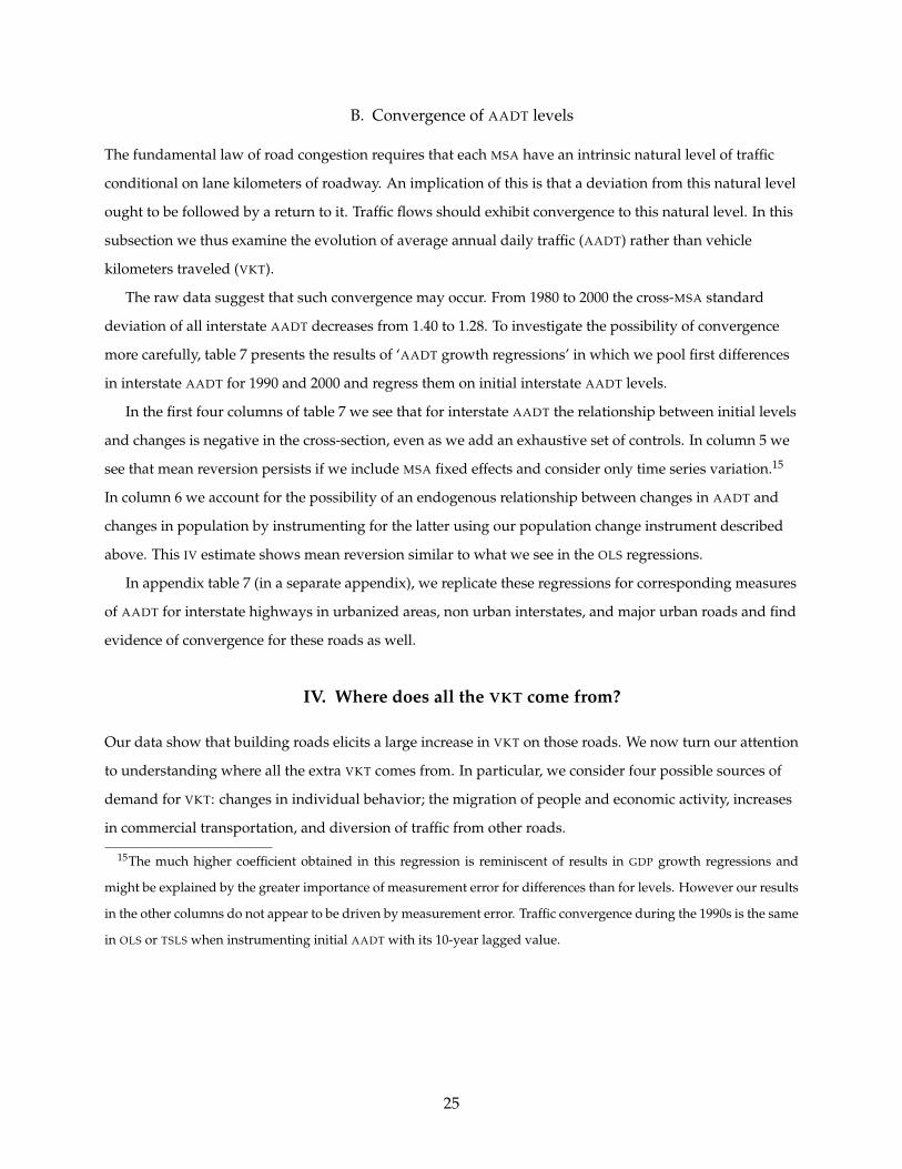
B. Convergence of AADT levels

The fundamental law of road congestion requires that each MSA have an intrinsic natural level of traffic

conditional on lane kilometers of roadway. An implication of this is that a deviation from this natural level

ought to be followed by a return to it. Traffic flows should exhibit convergence to this natural level. In this

subsection we thus examine the evolution of average annual daily traffic (AADT) rather than vehicle

kilometers traveled (VKT).

The raw data suggest that such convergence may occur. From 1980 to 2000 the cross-MSA standard

deviation of all interstate AADT decreases from 1.40 to 1.28. To investigate the possibility of convergence

more carefully, table 7 presents the results of ‘AADT growth regressions’ in which we pool first differences

in interstate AADT for 1990 and 2000 and regress them on initial interstate AADT levels.

In the first four columns of table 7 we see that for interstate AADT the relationship between initial levels

and changes is negative in the cross-section, even as we add an exhaustive set of controls. In column 5 we

see that mean reversion persists if we include MSA fixed effects and consider only time series variation.15

In column 6 we account for the possibility of an endogenous relationship between changes in AADT and

changes in population by instrumenting for the latter using our population change instrument described

above. This IV estimate shows mean reversion similar to what we see in the OLS regressions.

In appendix table 7 (in a separate appendix), we replicate these regressions for corresponding measures

of AADT for interstate highways in urbanized areas, non urban interstates, and major urban roads and find

evidence of convergence for these roads as well.

IV. Where does all the VKT come from?

Our data show that building roads elicits a large increase in VKT on those roads. We now turn our attention

to understanding where all the extra VKT comes from. In particular, we consider four possible sources of

demand for VKT: changes in individual behavior; the migration of people and economic activity, increases

in commercial transportation, and diversion of traffic from other roads.

15The much higher coefficient obtained in this regression is reminiscent of results in GDP growth regressions and

might be explained by the greater importance of measurement error for differences than for levels. However our results

in the other columns do not appear to be driven by measurement error. Traffic convergence during the 1990s is the same

in OLS or TSLS when instrumenting initial AADT with its 10-year lagged value.

25

TABLE 7—CONVERGENCE IN DAILY TRAFFIC.

[1] [2] [3] [4] [5] [6]OLS OLS OLS OLS OLS, FE TSLS

Dependent variable: Change in ln daily traffic (AADT) for interstate highways, entire MSAs.

Initial ln IH AADT level -0.11a -0.12a -0.17a -0.22a -0.98a -0.17a

(0.02) (0.02) (0.02) (0.03) (0.05) (0.02)

∆ ln(population) 0.38a 0.48a 0.29b 0.69b

(0.10) (0.11) (0.14) (0.31)Geography Y Y YCensus divisions Y Y YInitial share manufacturing Y YPast populations YSocio-econ. charac. Y

R2 0.26 0.32 0.39 0.44 0.82 -First stage Statistic 47.6

Notes: All regressions include decade effects. Robust standard errors in parentheses (clustered by MSA). 456observations corresponding to 228 MSAs for each regression. Instrument for ∆ ln(population) is expected populationgrowth based on initial composition of economic activity. interacted with the national growth of sectors.a: Significant at the 1 percent level.b: Significant at the 5 percent level.c: Significant at the 10 percent level.

A. Commercial VKT

To investigate the relationship between changes in the road network and changes in truck VKT we first use

the HPMS Sample data’s report of the daily share of single unit and combination trucks using each road

segment on an average day. With our other data, this allows us to calculate truck VKT for all roads in our

sample. With these measures of truck VKT in hand, we replicate our earlier analysis of all VKT for truck

VKT.

Table 8 reports these results. Our dependent variable is all interstate highway truck VKT and the

explanatory variable of interest is lane kilometers of interstate highways. In columns 1 through 5, we

report OLS estimates. In columns 6, 7 and 8 we include MSA fixed effects and identify the effect of interstate

highways on truck VKT using only time series variation. In columns 9 and 10 we report TSLS where we use

our three historical variables to instrument for contemporaneous lane kilometers. In every case, our

estimate of the highway elasticity of truck VKT is above one and is estimated precisely. While the OLS and

fixed-effect estimates are generally within two standard deviations of one, the IV estimates in columns 9

and 10 are above 2 and are more than two standard deviations above one.

In all, we find that a 10 percent increase in interstate highways causes about a 10-20 percent increase in

truck VKT, so that commercial traffic is at least as responsive to road supply as other traffic.

We confirm these results for all interstate highways in Appendix table 8 which runs separate regressions

for each decade. We also replicate these regressions for urbanized roads. Interestingly truck VKT in cities

26

TABLE 8—TRUCK VKT AS A FUNCTION OF LANE KILOMETERS, POOLED REGRESSIONS.

[1] [2] [3] [4] [5] [6] [7] [8] [9] [10]OLS OLS OLS OLS OLS OLS OLS OLS TSLS TSLS

Dependent variable: ln Truck VKT for interstate highways, entire MSAs

ln(IH lane km) 1.30a 1.16a 1.20a 1.25a 1.19a 1.46a 1.48a 1.52a 2.09a 2.32a

(0.07) (0.13) (0.13) (0.13) (0.14) (0.26) (0.27) (0.27) (0.44) (0.43)

ln(population) 0.16c 0.13 0.23b 1.79b 2.14b 2.02b -0.48 -0.77b

(0.08) (0.11) (0.10) (0.79) (0.94) (0.91) (0.31) (0.34)Geography Y Y Y YCensus divisions Y Y Y YSocio-econ. charac. Y Y YPast populations YMSA fixed effects Y Y Y

R2 0.53 0.54 0.58 0.59 0.61 0.31 0.34 0.34 - -Overidentification p-value 0.27 0.18First stage Statistic 16.5 11.8

Notes: All regressions include a constant and year effects. Robust standard errors clustered by MSA in parentheses.Instruments are ln 1835 exploration routes, ln 1898 railroads, and ln 1947 planned interstates. 684 observationscorresponding to 228 MSAs for each regression.a: Significant at the 1 percent level.b: Significant at the 5 percent level.c: Significant at the 10 percent level.

responds less to changes in major roads than does interstate truck traffic to changes in interstates.

In a separate appendix, we also examine the relationship between roads and employment in traffic

intensive activities. We use County Business Patterns data for 1983, 1993, and 2003. These data provide

county level information on employment in "Motor freight transportation and warehousing" (SIC 42).

Appendix tables 9 and 10 present results of regressions predicting log MSA employment in trucking and

warehousing. These regressions show that employment in this sector increases with interstate lane

kilometers, that it is more responsive to the supply of non urbanized area interstate than to the supply of

urbanized area interstate, and that it has become more sensitive to changes in the supply of interstate

highways over the course of our study period.

An interesting explanation for our findings is that improvements to highways cause large increases in

the use of these routes by long-haul truckers, while improvements to the local road network cause smaller

increases in local commercial traffic.

B. Individual driving behavior and highways

We now investigate the extent to which individual or household driving behavior changes in response to

changes in the extent of an MSA’s interstate network. To accomplish this, we look at the relationship

27

between lane kilometers of interstate highway and three different measures of individual and household

driving taken from the 1995 and 2001 NPTS.

The NPTS actually consists of four parts. The ‘household survey’ provides categorical variables

describing the age, race, education, and income of the household head or the principal respondent.16

Confidential geocode information allows us to assign all households to MSAs.17 The ‘vehicle survey’

provides a detailed description of each household motor vehicle including the survey respondents’ report

of how many kilometers it was driven in the past twelve months. We use the vehicle survey to construct an

estimate of total VKT for the household during the survey year. The ‘person survey’ describes travel

behavior for household members over the past week, commuting behavior in particular. We use the person

survey to measure commuting behavior for the average commuter in a respondent household. Finally, the

‘trip survey’ describes all household travel on a given randomly selected day. We use this survey to

measure all household daily VKT.

While we provide more detailed discussion of the NPTS and some descriptive statistics in the data

appendix, it is useful to discuss the relationship between the NPTS and HPMS based measures of VKT. The

NPTS reports a per household measure of VKT on all roads while the HPMS reports aggregate VKT on

interstates and major urban roads within MSAs. Thus, the HPMS looks at all traffic on a subset of roads

while the NPTS looks at all household driving on any roads, but ignores commercial or through traffic and

changes in population.

To investigate the extent to which individual or household driving behavior changes in response to

changes in the extent of an MSA’s interstate network we look at the relationship between lane kilometers of

interstate highway and our three NPTS derived measures of individual and household driving.

We perform two series of estimations using our two pooled cross-sections of the NPTS. The first uses

our city level cross-section estimating equation (2), adjusted to reflect the fact that our unit of observation is

16It is worth noting that the NPTS survey protocol requires a phone call, a house visit, and that respondents keep a

travel diary. Thus it should be regarded as accurate relative to other sources self-reported travel data. The 2000 US census

provides an alternative source of information regarding commute times. This information is reported for a sample of

the population using 12 time-bands. A comparison between 2000 census and 2001 NPTS data of mean commute times

across 227 MSAs yields a raw correlation of 0.63. This correlation is 0.85 when considering only MSAs with population

above 1 million. Means computed from the NPTS appear more noisy. Regressing log census mean commute times for

all commuters (including those using public transportation) against mean NPTS car commute times yields a coefficient

of 1.05 in a regression without constant.17The public use data only reveals respondents’s MSAs for respondents residing in large MSAs. We do not use earlier

waves of the NPTS because they cannot be geocoded.

28

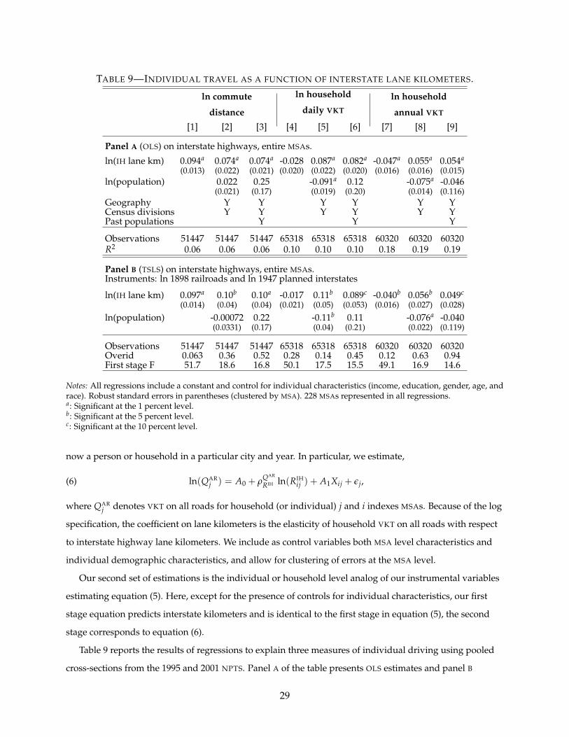
TABLE 9—INDIVIDUAL TRAVEL AS A FUNCTION OF INTERSTATE LANE KILOMETERS.

ln commute

distance

ln household

daily VKT

ln household

annual VKT

[1] [2] [3] [4] [5] [6] [7] [8] [9]

Panel A (OLS) on interstate highways, entire MSAs.

ln(IH lane km) 0.094a 0.074a 0.074a -0.028 0.087a 0.082a -0.047a 0.055a 0.054a

(0.013) (0.022) (0.021) (0.020) (0.022) (0.020) (0.016) (0.016) (0.015)ln(population) 0.022 0.25 -0.091a 0.12 -0.075a -0.046

(0.021) (0.17) (0.019) (0.20) (0.014) (0.116)Geography Y Y Y Y Y YCensus divisions Y Y Y Y Y YPast populations Y Y Y

Observations 51447 51447 51447 65318 65318 65318 60320 60320 60320R2 0.06 0.06 0.06 0.10 0.10 0.10 0.18 0.19 0.19

Panel B (TSLS) on interstate highways, entire MSAs.Instruments: ln 1898 railroads and ln 1947 planned interstates

ln(IH lane km) 0.097a 0.10b 0.10a -0.017 0.11b 0.089c -0.040b 0.056b 0.049c

(0.014) (0.04) (0.04) (0.021) (0.05) (0.053) (0.016) (0.027) (0.028)

ln(population) -0.00072 0.22 -0.11b 0.11 -0.076a -0.040(0.0331) (0.17) (0.04) (0.21) (0.022) (0.119)

Observations 51447 51447 51447 65318 65318 65318 60320 60320 60320Overid 0.063 0.36 0.52 0.28 0.14 0.45 0.12 0.63 0.94First stage F 51.7 18.6 16.8 50.1 17.5 15.5 49.1 16.9 14.6

Notes: All regressions include a constant and control for individual characteristics (income, education, gender, age, andrace). Robust standard errors in parentheses (clustered by MSA). 228 MSAs represented in all regressions.a: Significant at the 1 percent level.b: Significant at the 5 percent level.c: Significant at the 10 percent level.

now a person or household in a particular city and year. In particular, we estimate,

ln(QARj ) = A0 + ρQAR

RIH ln(RIHij ) + A1Xij + εj,(6)

where QARj denotes VKT on all roads for household (or individual) j and i indexes MSAs. Because of the log

specification, the coefficient on lane kilometers is the elasticity of household VKT on all roads with respect

to interstate highway lane kilometers. We include as control variables both MSA level characteristics and

individual demographic characteristics, and allow for clustering of errors at the MSA level.

Our second set of estimations is the individual or household level analog of our instrumental variables

estimating equation (5). Here, except for the presence of controls for individual characteristics, our first

stage equation predicts interstate kilometers and is identical to the first stage in equation (5), the second

stage corresponds to equation (6).

Table 9 reports the results of regressions to explain three measures of individual driving using pooled

cross-sections from the 1995 and 2001 NPTS. Panel A of the table presents OLS estimates and panel B

29

presents TSLS estimates. In the first three columns our dependent variable is commute kilometers on a

typical day for all NPTS individuals who commute. In columns 4 through 6 our dependent variable is total

household vehicle kilometers on a particular travel day. In columns 7 through 9, our dependent variable is

total VKT by all household vehicles in the survey year.

With the exception of the regression in column 7, for which there is no measurable relationship between

interstate kilometers and household vehicle kilometers, all estimates suggest a positive and statistically

significant relationship between the extent of the highway network and individual travel. Our preferred

estimates are the TSLS estimates in panel B. These estimates suggest that a 10 percent increase in the extent

of the interstate network causes about a 1 percent increase in individual driving on all roads. While the

NPTS data does not reveal which classes of roads accommodate this increase in driving, below we use the

HPMS to explore the diversion of traffic between classes of roads.

C. Population growth

By reducing the cost of transportation within a city, all else equal, improvements to a city’s road network

make a city more attractive relative to other cities. Given the high mobility of the US population, this

suggests that changes to a city’s road network should be met with changes to a city’s population. In fact,

this conjecture appears to be true, and the extant literature estimates the size of this effect.

Michaels (2008) and Amitabh Chandra and Eric Thompson (2000) provide suggestive evidence. Both

papers consider the effect of improvements in access to the interstate system on rural counties in the US.

Michaels (2008) finds that an interstate highway in a rural county leads to large increases in retail earnings.

Chandra and Thompson (2000) find that improved access to the interstate system causes an overall

increase in firm earnings. Together, these results show that interstate highways cause increases in the level

of local economic activity. To the extent that population levels and overall economic activity are linked, this

suggests that improvements to the interstate network lead to population increases.

Duranton and Turner (2008) provide more direct evidence. Duranton and Turner (2008) consider US

MSAs between 1980 and 2000, and investigate the way that population growth responds to changes in the

road network. Like the current paper, they rely on an early plan of the interstate highway network and

1898 railroad routes as instruments for the modern road network. They find that a 10 percent increase the

extent of the road network causes a 1.3 percent increase in MSA population over 10 years, and a 2 percent

increase over 20 years.

30

D. Diversion from other roads

We measure traffic and lane kilometers for three exclusive classes of roads in each MSA; urbanized area

interstates, non urbanized area interstates, and major urbanized area roads. These data allow direct tests of

whether changes to one class of roads affects VKT on the others. In particular, we estimate each of the three

following variants of equation (2),

ln(QIHUit ) = A0 + ρQIHU

RIHU ln(RIHUit ) + ρQIHU

RIHNU ln(RIHNUit ) + ρQIHU

RMRU ln(RMRUit ) + A1Xit + εit(7)

ln(QIHNUit ) = B0 + ρQIHNU

RIHU ln(RIHUit ) + ρQIHNU

RIHNU ln(RIHNUit ) + ρQIHNU

RMRU ln(RMRUit ) + B1Xit + γit(8)

ln(QMRUit ) = C0 + ρQMRU

RIHU ln(RIHUit ) + ρQMRU

RIHNU ln(RIHNUit ) + ρQMRU

RMRU ln(RMRUit ) + C1Xit + νit.(9)

In equation (7), ρQIHU

RIHNU is the urbanized area interstate VKT elasticity of non urbanized area interstate lane

kilometers. If, for example, this parameter is -0.1 then a 10 percent increase in non urbanized area interstate

lane kilometers results in a 1 percent decrease in urbanized area interstate VKT. Interpretation of other

coefficients is similar.

Table 10 reports estimates of equations (7)-(9). In all regressions we pool our three cross-sections of

HPMS data and use OLS. Panel A presents estimates of equation (7). In these regressions our dependent

variable is urbanized area interstate VKT and the dependent variables of interest are the three measures of

lane kilometers. We exploit cross-sectional variation and from left to right, use progressively more

exhaustive lists of controls. Panels B and C are similar to panel A, but use non urbanized interstate VKT and

major urbanized area road VKT as dependent variables.

Consistent with our earlier results we see that VKT elasticity of own lane kilometers is close to one for

all specifications in panel A and above 0.8 for all specifications in panels B and C. The largest estimated

cross elasticity is 0.22 for the non urbanized area interstate VKT elasticity of urbanized area major road lane

kilometers, in column 1, row 3 of panel B. This estimate is not robust to the addition of controls, and is

negative or indistinguishable from zero in other specifications. The estimate of the urbanized area

interstate VKT elasticity of urbanized area major road lane kilometers in row 3 column 1 of panel A is

similar. Other cross-elasticities are generally quite small. Our preferred regressions are reported in column

5. In this specification, all cross-elasticities are negative with magnitudes no larger than 0.1. In sum, table

10 suggests that, while traffic diversion does occur in response to changes in the road network, the

fundamental law of road congestion mainly reflects traffic creation rather than traffic diversion.

In a separate appendix, we confirm these results in appendix tables 11 and 12. In these tables we

replicate the results of table 10 in decade by decade OLS regressions and in first difference regressions.

31

TABLE 10—VKT AS A FUNCTION OF LANE KILOMETERS FOR DIFFERENT TYPES OF ROADS, POOLED

OLS.

[1] [2] [3] [4] [5]

Panel A. Dependent variable: ln VKT for interstate highways, urbanized areas within MSAs

ln(IHU lane km) 1.09a 1.01a 1.04a 1.03a 1.04a

(0.03) (0.03) (0.03) (0.03) (0.03)ln(IHNU lane km) -0.026 -0.083a -0.086a -0.087a -0.099a

(0.031) (0.025) (0.024) (0.024) (0.023)

ln(MRU lane km) 0.22a -0.13b -0.12b -0.12b -0.100b

(0.04) (0.06) (0.06) (0.05) (0.05)ln(population) Y Y Y YGeography Y Y YCensus divisions Y Y YSocio-econ. charac. Y YPast populations Y

R2 0.96 0.97 0.97 0.98 0.98

Panel B. Dependent variable: ln VKT for interstate highways, outside urbanized areas within MSAs

ln(IHU lane km) 0.032 -0.049 -0.030 -0.030 -0.013(0.037) (0.034) (0.031) (0.030) (0.032)

ln(IHNU lane km) 0.87a 0.81a 0.84a 0.85a 0.83a

(0.04) (0.03) (0.03) (0.02) (0.02)

ln(MRU lane km) 0.22a -0.14b -0.053 -0.046 -0.013(0.05) (0.05) (0.052) (0.050) (0.050)

R2 0.85 0.88 0.92 0.92 0.93

Panel C. Dependent variable: ln VKT for Major Roads, urbanized areas within MSAs

ln(IHU lane km) 0.015 -0.049a -0.049a -0.057a -0.048a

(0.021) (0.018) (0.016) (0.014) (0.015)

ln(IHNU lane km) 0.042b -0.0038 0.00063 -0.0044 -0.0042(0.021) (0.0181) (0.0150) (0.0133) (0.0133)

ln(MRU lane km) 1.09a 0.81a 0.82a 0.81a 0.82a

(0.03) (0.03) (0.03) (0.03) (0.03)

R2 0.97 0.98 0.99 0.99 0.99

Notes: All regressions include a constant and year effects. Robust standard errors clustered by MSA in parentheses. 572observations corresponding to 192 MSAs for each regression.a: Significant at the 1 percent level.b: Significant at the 5 percent level.c: Significant at the 10 percent level.

32

E. An accounting exercise

The fundamental law of road congestion requires that changes in the extent of the road network are met

with proportional changes in traffic. We have suggested four possible sources for this increase in traffic;

changes in trucking and commercial driving, changes in individual or household driving behavior,

changes in population, and diversion of traffic. We now consider whether these four sources are sufficient

to explain the fundamental law and assess their relative importance.

To begin, consider a 10 percent increase in the interstate network of an average MSA around 2000. Using

our preferred estimate from column 3 of table 5, this increase causes a 10.3 percent increase in VKT on the

interstates of our hypothetical city.

In table 1 we see that in 2003, trucks accounted for 13 percent of VKT on interstate highways in an

average MSA. In table 8, our preferred specification is column 10, where the truck VKT elasticity of

interstate highways is about 2.3. This means that a 10 percent increase in the stock of roads causes about a

23 percent increase in truck VKT and a 3.0 percent increase in overall interstate VKT, about 29 percent of the

total increase in VKT caused by our 10 percent increase in roads. While our preferred elasticity of 2.3 may

seem high, the average of all estimates in panel A of table 8 is 1.5. This lower value would imply that trucks

represent 18 percent of the total increase in VKT. Therefore, we estimate that trucks account for between 19

and 29 percent of the total increase in interstate VKT that results from our hypothetical 10 percent increase

in interstate lane kilometers.

For migration, taking the preferred estimate from Duranton and Turner (2008), our 10 percent increase

in the interstate network causes about a 2.1 percent increase in population. From column 3 of table 5, the

MSA population elasticity of interstate VKT is 0.30. Together, these two elasticities suggest that a 10 percent

increase in population results in about a 0.6 percent increase interstate VKT, about 6 percent of the total

increase. This elasticity of 0.30 is estimated in a regression that also controls for decennial population levels

between 1920 and 1970. Because decennial population levels are highly correlated, this may understate the

effect of population on VKT.

Panel B of table 4, which controls for the endogeneity of population in first difference estimates, reports

higher estimates. The estimate in column 5 is 1.02. This alternative value implies that population growth

represents 21 percent the total effect of an extension in interstate lane kilometers. Therefore, we estimate

that migration accounts for between 5 and 21 percent of the total increase in interstate VKT that results from

our hypothetical 10 percent increase in interstate lane kilometers.

Turning to substitution across roads, we suppose that the 10 percent increase in our MSA’s interstate

lane kilometers network is accomplished by increasing both urbanized and non urbanized interstates by 10

percent. Since we are considering increases to both classes of interstate highways, we need only be

33

concerned with diversion of traffic from major urbanized area roads. This is estimated in panel C of table

10. In rows 1 and 2 of column 5, we see that a 10 percent increase in urbanized and non urbanized

interstate causes a decrease in major urban road VKT of 0.48 percent and 0.04 percent, respectively (and

basing our calculation on column 3 or 4 would yield similar results). That is, our 10 percent increase in

interstate lane kilometers diverts 0.52 percent of traffic from major urban roads. Using the levels of VKT for

major urban and all interstates given in table 1 allows us to calculate that this diversion amounts to about a

1 percent increase in interstate VKT, or about 10 percent of the total effect of our hypothetical 10 percent

extension. Because many estimates in table 10 (or in appendix tables 12 and 13) indicate no substitution

from major urban roads towards interstates, we cannot rule out the absence of a substitution effect.

Therefore, we estimate that the diversion of traffic from other classes of roads accounts for between 0 and

10 percent of the total increase in interstate VKT that results from our hypothetical 10 percent increase in

interstate lane kilometers.

Calculating the contribution of changes to household behavior is more difficult. Table 9 estimates the

effect of interstate lane kilometers on individual driving behavior. We take the estimate of 0.11 given by

column 5 of panel B (which is very close to the corresponding estimate for alternative measures of VKT in

columns 2, 3, and 6 of both panels). A 10 percent increase in interstate lane kilometers causes a 1.1 percent

increase in household annual VKT. Unfortunately, our data do not allow us to apportion household driving

to different road networks. A first possibility is to assume that this 1.1 percent increase in driving is

proportional to current driving across all road networks. Since households represent 87 percent of

interstate VKT, this 1.1 percent increase represents an increase in interstate VKT of 0.9 percent or 9 percent

of the total increase in interstate VKT caused by a 10 percent increase in lane kilometers. This is arguably an

unrealistic lower bound. Alternately, suppose that the 1.1 percent increase in household driving takes

place only on interstates (recall that we earlier reported that about 24 percent of VKT takes place on

interstates). In this case, the increase in interstate VKT would account for 4.1 percent of the total change in

VKT or 39 percent of the effect of our expansion in lane miles. This constitutes an upper-bound. Therefore,

we estimate that increases in household driving account for between 9 and 39 percent of the total increase

in interstate VKT that results from our hypothetical 10 percent increase in interstate lane kilometers.

To sum up, of four possible sources for the new traffic following an increase in lane kilometers of

interstates, changes to individual behavior and changes in commercial driving are the most important.

Migration and traffic diversion are significantly less important. We also note that if we take the upper

bounds for the shares of all four sources we account for just about the entire increase in VKT.

34

V. Conclusion

This paper analyzes new data describing city level traffic in the continental US between 1983 and 2003. Our

estimates of the elasticity of MSA interstate highway VKT with respect to lane kilometers are 0.86 in OLS,

1.00 in first difference, and 1.03 with IV. Because our instruments provide a plausible source of exogenous

variation, we regard 1.03 as the most defensible estimate. We take this as a confirmation of the

‘fundamental law of highway congestion’ suggested by Downs (1962) where the extension of interstate

highways is met with a proportional increase in traffic for US MSAs.

We also provide suggestive evidence that this law extends beyond urban highways, a ‘fundamental law

of road congestion’. For a broad class of major roads within the ‘urbanized’ part of MSAs we estimate a

roadway elasticity of VKT between 0.67 and 0.89 depending on the decade in OLS. Changes in the

boundaries of urban areas over time and the weakness of our instruments for this class of roads preclude

reliable first-difference and IV estimates.

Beyond direct evidence we confirm two implications of the fundamental law of road congestion; we

find no evidence that public transit affects VKT and there is convergence of traffic levels. Our results also

suggest that roads are assigned to MSAs with little or no regard for the prevailing level of traffic.

We also consider the sources of new traffic elicited by extensions to the interstate network. We find that

changes to individual driving behavior and increases in trucking are most important. Migration is

somewhat less important. Surprisingly, diversion of traffic from other road networks does not appear to

play a large role.

These findings suggest that both road capacity expansions and extensions to public transit are not

appropriate policies with which to combat traffic congestion. This leaves congestion pricing as the main

candidate tool to curb traffic congestion.

35

REFERENCES

Bartik, Timothy. 1991. Who Benefits from State and Local Economic Development Policies? Kalamazoo (MI):

W.E. Upjohn Institute for Employment Research.

Baum-Snow, Nathaniel. 2007. “Did Highways Cause Suburbanization?” Quarterly Journal of Economics

122(2): 775–805.

Burchfield, Marcy, Henry G. Overman, Diego Puga, and Matthew A. Turner. 2006. “Causes of Sprawl: A

Portrait from Space.” Quarterly Journal of Economics 121(2): 587–633.

Cervero, Robert. 2002. “Induced Travel Demand: Research Design, Empirical Evidence, and Normative

Policies.” Journal of Planning Literature 17(3): 2–20.

Cervero, Robert, and Mark Hansen. 2002. “Induced Travel Demand and Induced Road Investment: A

Simultaneous Equation Analysis.” Journal of Transport Economics and Policy 36(3): 469–490.

Chandra, Amitabh, and Eric Thompson. 2000. “Does Public Infractsructure Affect Economic Activity?

Evidence from the Rural Interstate Highway System.” Regional Science and Urban Economics 30(4):

457–490.

Cutler, David M., and Edward L. Glaeser. 1997. “Are Ghettos Good or Bad?” Quarterly Journal of

Economics 112(3): 827–872.

Downs, Anthony. 1962. “The Law of Peak-Hour Express-Way Congestion.” Traffic Quarterly 16(3): 393–409.

Downs, Anthony. 1992. Stuck in Traffic: Coping With Peak-Hour Traffic Congestion. Washington D.C.:

Brookings Institution Press.

Dupuit, Jules E.J. 1844. “De la Mesure de l’Utilité des Travaux Publics.” Annales des Ponts et Chaussées

Second series, 8(116): 332–375.

Duranton, Gilles, and Matthew A. Turner. 2008. “Urban Growth and Transportation.” Unpublished.

Duranton, Gilles, and Matthew A. Turner. 2009. “The Fundamental Law of Road Congestion: Evidence

From US Cities.” National Bureau of Economic Research Working Paper 15376.

Fernald, John G. 1999. “Roads to Prosperity? Assessing the Link between Public Capital and

Productivity.” American Economic Review 89(3): 619–638.

Ferreira, Fernando, and Joseph Gyourko. 2009. “Do Political Parties Matter? Evidence from US Cities.”

Quarterly Journal of Economics 124(1): 399–422.

36

Fishlow, Albert. 1965. American Railroads and the Transformation of the Ante-Bellum Economy. Cambridge

(MA): Harvard University Press.

Fogel, Robert. 1964. Railroads and American Economic Growth: Essays in Econometric History. Baltimore (MD):

Johns Hopkins University Press.

Fulton, Lewis M., Robert B. Noland, Daniel J. Meszler, and John V. Thomas. 2000. “A Statistical Analysis

of Induced Travel Effects in the U.S. Mid-Atlantic Region.” Journal of Transportation Statistics 3(1) :1–14.

Glaeser, Edward L., José A. Scheinkman, and Andrei Shleifer. 1995. “Economic Growth in a

Cross-Section of Cities.” Journal of Monetary Economics 36(1): 117–143.

Gomez-Ibanez, Jose A. 1996. “Big-City Transit, Ridership, Deficits, and Politics.” Journal of the American

Planning Association 62(1): 30–50.

Goodwin, Phil B. 1996. “Empirical Evidence on Induced Traffic.” Transportation 23(1): 23–54.

Gray, Charles P. c. 1898. Gray’s New Trunk Railway Map of the United States, Dom. of Canada and Portion of

Mexico. Compiled from latest official sources, showing carefully selected list of cities & towns in readable type for

quick reference. New York, NY. Library of congress catalogue # G3701.P3 1898 G7 RR 67.

Hansen, Mark, David Gillen, Allison Dobbins, Yualin Huang, and Monish Puvathingal. 1993. “The Air

Quality Impacts of Urban Highway Capacity Expansion: Traffic Generation and Land Use Changes.”

Report, University of California at Berkeley, Institute for Transportation Studies.

Hansen, Mark and Yuanlin Huang. 1997. “Road Supply and Traffic in California Urban Areas.”

Transportation Research A 21(3): 205–218.

Hess, Daniel Baldwin, and Peter A. Lombardi. 2005. “Governmental Subsidies for Public Transit: History,

Current Issues, and Recent Evidence.” Public Works Management Policy 10(4): 138–156.

Jorgensen, Roy E. 1947. “Influence of Expressways in Diverting Traffic from Alternate Routes and in

Generating New Traffic.” Highway Research Board Proceedings, Traffic and Operations 27(0): 322–330.

Koppelman, Frank S. 1972. “Preliminary Study for Development of a Macro Urban Transport Travel

Demand Model.” Technical report, Massachussets Institute of Technology, Department of Civil

Engineering, Transportation System Division.

Krueger, Alan B., Daniel Kahneman, David Schkade, Norbert Schwarz, and Arthur A. Stone. 2009.

“National Time Accounting: The Currency of Life.” In Alan B. Krueger (ed.) Measuring the Subjective

37

Well-Being of Nations: National Accounts of Time Use and Well-Being. Chicago: NBER and University of

Chicago Press, 9–86.

Michaels, Guy. 2008. “The Effect of Trade on the Demand for Skill - Evidence from the Interstate Highway

System.” Review of Economics and Statistics 90(4): 683–701.

Noland, Robert B. 2001. “Relationship between Highway Capacity and Vehicle Travel.” Transportation

Research A 35(1): 47–72.

Noland, Robert B., and William A. Cowart. 2000. “Analysis of Metropolitan Highway Capacity and the

Growth in Vehicle Miles of Travel.” Transportation 27(4): 363–390.

Schipper, Mark, and Vicki Moorhead. 2000. “Odometer versus Self-Reported Estimates of Vehicle Miles

Traveled.” Technical Document, Energy Information Administration (United States Department of

Energy).

Small, Kenneth A., and Erik T. Verhoef. 2007. The Economics of Urban Transportation. New York (NY):

Routledge.

Stock, James H., and Motohiro Yogo. 2005. “Testing for Weak Instruments in Linear IV Regression.” In

Donald W.K. Andrews and James H. Stock (eds.) Identification and Inference for Econometric Models: Essays

in Honor of Thomas Rothenberg. Cambridge: Cambridge University Press, 80–108.

US Bureau of Transportation Statistics. 2007. Transportation Statistics Annual Report 2007. Washington, DC:

US Government Printing Office.

US Department of Transportation, Federal Highway Administration. 1989. FHWA Functional Classification

Guidlines. Washington, DC: US Government Printing Office.

US Department of Transportation, Federal Highway Administration. 2003a. Archive Highway Performance

Monitoring System (HPMS) Data Item Descriptions 1993 - 1998. Washington, DC: US Government Printing

Office.

US Department of Transportation, Federal Highway Administration. 2003b. Archive Highway Performance

Monitoring System (HPMS) Data Item Descriptions 1982-1987. Washington, DC:: US Government Printing

Office.

US Department of Transportation, Federal Highway Administration. 2005a. Highway Statistics 2005,

Functional System Travel, Table VM-2. Washington, DC:: US Government Printing Office.

38

US Department of Transportation, Federal Highway Administration. 2005b. HPMS Field Manual.

Washington, DC:: US Government Printing Office.

US Department of Transportation, Urban Mass Transit Administration. 1986. National Urban Mass Transit

Statistics, 1984 Section 15 report. Washington, DC: US Government Printing Office.

US Federal Works Agency, Public Roads Administration. 1947. Press release.

US Geological Survey. 1970. The National Atlas of the United States of America. Washington, DC: United

States Geological Survey.

US House of Representatives. 1947. A Report on the National Interregional Highway Committee, Outlining and

Recommending a National System of Interregional Highways. Washington, DC: US Government Printing

Office.

Weiner, Edward. 1997. Urban Transportation Planning in the United States: An Historical Overview. Fifth

edition. Washington, DC: US Department of Transportation.

Wooldridge, Jeffrey M. 2001. Econometric Analysis of Cross Section and Panel Data. First edition. Cambridge

MA: MIT press.

APPENDIX A: DESCRIPTION OF DATA

A.. Consistent MSA definitions

MSA’s are defined as aggregations of counties. We use the 1999 MSA definitions. In order to insure that our

definitions are constant over time, we track changes in county boundaries back to 1920 and make

adjustments to MSA definitions as required in each decade.

B.. HPMS data

We rely extensively on the Highway Performance Monitoring System (HPMS) data for 1983, 1993, and 2003,

and slightly on the HPMS data for 1995 and 2001. These data are collected and maintained by the US

Federal Highway Administration in cooperation with many sub-national government agencies.

Documentation is available in DOT (2003a, 2003b, and 2005b).

The HPMS consists of two parts. The Universe data is supplied for most road segments in the interstate

highway system and some other major roads, and provides a description of each segment. The Sample data

provides additional information about all segments in the Universe data, including an urbanized area code

39

for segments falling in urbanized areas. For a sample of smaller urbanized area roads, the Sample data also

provides all data fields that occur in the Universe and Sample data.

In general, each segment reported in the HPMS represents a larger set of similar segments (typically of

the same road), called a sample. Thus, each reported segment is associated with an expansion factor which

relates the length of the segment described in the data to the length of the sample it represents. Since states

are required to report information on every interstate highway segment, all interstate highway segments

should have an expansion factor of one. In fact, the average expansion factor for these segments is about

1.5, so that states seem not to be in compliance with reporting requirements. For non interstate segments,

principally smaller classes of roads, reporting requirements permit expansion factors of up to 100. In fact, a

small number of larger expansion factors occur but we exclude these segments from our sample. For

urbanized area roads in the relevant classes, reporting rules require that the union of all samples be the set

of all urbanized area roads. Loosely, urbanized area road segments are partitioned into sets of similar

segments, and one segment from each set is reported in the HPMS sample data. In this sense, Sample data

represents all urbanized road segments subject to reporting requirements.

For the interstate highway system the HPMS records number of lanes, length, AADT, and county. By

construction, road segments do not cross county borders. For segments in urbanized areas, the HPMS also

provides an urbanized area code. Since MSAs are county based units, these data allow us to calculate VKT

for the urbanized and non urbanized area interstate systems by MSA.

Within urbanized areas, the HPMS, not only describes the interstate highway system, but also all roads

in the following functional classes: Principal arterial - Other freeways and expressways, Principal arterial -

other, Minor arterial, Collector, Local. There is no mandated reporting of local roads, so they make up only

a small share of the HPMS data and are excluded from our analysis. Our ‘major roads’ are defined as the

union of the remaining classes. The definitions of these road classes are given in DOT (1989) and span

about 20 pages. Loosely, a local road is one which is predominantly used to access addresses on that road,

e.g., a residential street. Any road used principally to connect local roads (but not an interstate) falls in one

of the larger classes that we consolidate into major roads.

C.. NPTS data

In table 11, we report some descriptive statistics about our two waves of the NPTS. Surprisingly, these data

show that driving distances per person, household, and vehicle all declined between 1995 and 2001.

The ‘vehicle survey’ provides a detailed description of each household motor vehicle including the

survey respondents’ report of how many kilometers it was driven in the past twelve months. We use this

information to construct an estimate of total VKT for the household during the survey year. This

40

information is reported in the top section of table 11. The ‘person survey’ describes travel behavior for each

household member on a typical travel day. From this, we construct household mean commute distance,

time and speed for household members who drive to work. Table 11 shows that mean commute distance

decreased from 20.4 km in 1995 to 19.4 in 2001. This decrease in distance resulted in a small decrease in

mean commute times despite a decline in speed. Finally, the ‘travel day’ survey collects detailed

information about each trip taken by each household member on a randomly selected travel day. These

data allow the calculation of household person-kilometers of vehicle travel, along with the person-minutes

required to accomplish this travel, and the average speed of this travel. Table 11 shows that total daily

household person-kilometers of travel was approximately constant over the study period, but that the time

required to accomplish this travel increased from 147.7 minutes to 160.9 minutes and speed decreased from

48.4 to 43.9 km/h.

The descriptive statistics in table 11 point at stability or a small decline in VKT per household between

1995 and 2001. For the same period, the HPMS indicates increases of around 20 percent for VKT, as reported

at the bottom of table 11. It is natural to wonder whether these two findings are contradictory. To see that

they are not, note that the NPTS and the HPMS report different measures of VKT.18 The NPTS reports a per

household measure of VKT on all roads. On the other hand, the HPMS reports aggregate VKT on interstates

and major urban roads within MSAs. Thus, the HPMS looks at a different set of roads than the NPTS and the

2001-1995 difference reflects changes in commercial traffic and number of households, in addition to

changes in VKT per household.

D.. Instruments

Our measures of the 1947 interstate highway plan and the 1898 railroad network are taken from Duranton

and Turner (2008) and are documented there. Further discussion of the 1947 highway plan is available in

Michaels (2008) and Baum-Snow (2007).

While our exploration routes variable is new, Duranton and Turner (2008) experimented with a

different formulation and found that it did not have much predictive ability. In this initial formulation of

the exploration route data, we treated the exploration route map in exactly the same way as we did the

1947 highway plan and the 1898 railroad map. That is, all routes are treated in exactly the same way and

18We rule out sampling errors. NPTS data sample a large number of households, are broadly acknowledged to be

of high quality, and their correlation with census data is also high as mentioned above. Mark Schipper and Vicki

Moorhead (2000) also provide evidence that reported VKT in the NPTS is highly consistent with odometer VKT from the

1994 Residential Transportation Energy Consumption Survey. As for the HPMS, it is carefully scrutinized by the Bureau

of Transportation Statistics which uses it as the basis of its Transportation Statistics Annual Report.

41

TABLE 11—SUMMARY STATISTICS FOR OUR MAIN NPTS VARIABLES AND HMPS VKT FOR CORRES-

PONDING YEARS.

Year: 1995 2001

NPTS vehicle survey (annual)Mean vehicle km (person) 12,436 12,203

(7,737) (8,398)Mean vehicle km (household) 32,546 30,352

(19,672) (20,198)Mean vehicle km (vehicle) 19,560 17,573

(9,355) (9,030)

NPTS person survey (daily)Distance to work (km) 20.4 19.4

(21.6) (20.2)Minutes drive to work 22.4 21.3

(17.3) (16.3)Speed to work 50.9 49.6

(21.1) (22.1)

NPTS trip survey (daily)Total household person-km 134.8 134.5

(119.9) (112.0)Total household person-minutes 147.7 160.9

(88.7) (90.7)Mean household km/h 48.4 43.9

(12.2) (15.1)

Total HMPS VKT

Interstate Highways (’000 km) 2,876,074 3,484,750Major Urban Roads (’000 km) 5,530,845 6,624,656

Number MSAs 228 228

Notes: Averaged over individuals or households. Means and standard deviations between brackets.

receive exactly the same weight. In particular, this means that well used and important routes, such as the

Oregon or Santa Fe trails, are given the same weight as less successful routes. With this said, since the

exploration routes map provides a line for each expedition it describes, even if this line is very close to the

line for another expedition on the same route, the map does permit us to distinguish more intensively used

routes from less. In particular, if we digitize the map and count all pixels assigned to any route, we have a

measure of the intensity with which a region was used by explorers between 1835 and 1850. This is

precisely what we did. Figure 5 illustrates.

The share of the democratic vote in the 1972 presidential election is calculated from the General Election

Data for the United States, 1950-1990, from the Inter-university Consortium for Political and Social

42

FIGURE 5—CONSTRUCTION OF AN EXPLORATION ROUTES INDEX

Notes: Right panel gives detail of original map of 1835-1850 exploration routes for a segment of the Oregon trail nearSalt Lake City (US Geological Survey, 1970). Left panel shows incidence of exploration routes in same region. For thisregion, our measure of exploration routes is the count of grey pixels in the right panel.

Research (ICPSR).

E.. Geography

Our data includes five measures describing the physical geography of an MSA taken from the data used by

Marcy Burchfield et al. (2006). The particular measures of physical geography that we use are: elevation

range within the MSA, the ruggedness of terrain in the MSA, heating degree days, and cooling degree days

and ‘sprawl’ in 1992. Elevation range is the difference in meters between the elevation of the highest and

lowest point in the MSA. Ruggedness is calculated by imposing a regular 90 meter grid on each MSA and

calculating the mean difference in elevation between each cell and adjacent cells. Heating and cooling

degree days are engineering measures used to assess the demand for heating and cooling. Sprawl is the

measure of sprawl calculated in Burchfield et al. (2006) and measures the share of undeveloped land in the

square kilometer surrounding an average structure. More detail about these variables is available in

Burchfield et al. (2006) and at http://diegopuga.org/data/sprawl/.

F.. Employment

To measure employment we use the County Business Patterns data from the US Census Bureau. These data

are available annually from 1983 to 2003. We construct disaggregated employment data at the two

digit-level (with 81 sectors) to investigate whether the supply of interstate highways and other major roads

affects the composition of economic activity and, in particular, employment in transportation-intensive

sectors. Between 1983 and 2003, three different industrial classifications have been used in the US: the

43

standard industrial classification (SIC) which remained unchanged at the two-digit level until 1997, the

1997 North American Industry Classification System (NAICS) from 1998 to 2002, and the 2002 NAICS for

2003. Using the same cross-walk as in Duranton and Turner (2008), we perform our employment

regressions using SIC categories.

G.. Public transit infrastructure

To comply with Section 15 of the Urban Mass Transportation Act, all public transit districts in the US

submit annual reports to the federal government detailing their assets and activities over the course of the

year. Our data for 1984 bus service comes from table 3.6, p3-308, of DOT Urban Mass Transit

Administration (1986). The section 15 reports are available in electronic form starting in 1984. While these

reports do not assign transit districts to an MSA, they contain enough geographic information, e.g.,

zipcode, so that about 700 of the 740 transit districts that operate during 1984, 1994, or 2004 can be assigned

to a non MSA county or to an MSA.

With this correspondence constructed, we count all ‘large buses’ in each MSA at peak service for 1984.

We use this daily average number of large buses operating at peak service in 1984 to measure an MSA’s

stock of public transit infrastructure. In our definition of large buses we include buses in the following

Section 15 reporting classes: articulated bus; bus A (>35 seats); bus B (25-35 seats); bus C (<25 seats);

double deck bus; motor bus; motor bus (private); street car; trolley bus.

H.. Socio-economic characteristics:

To measure MSA socio-economic characteristics, we use three data sources. The share of manufacturing

employment is computed from the County Business Patterns for 1983, 1993, and 2003 to match the years of

data for VKT and roadway. The 1980 segregation index is calculated from 1980 census tract level data and is

based on the measure of housing segregation described in equation (3), p. 836 of David M. Cutler and

Glaeser (1997). Finally, the share of college educated workers, share of poor, and average earnings are

computed using data from the 1980, 1990, and 2000 decennial censuses. From the education questions in

these three censuses, we are able to build a consistent variable capturing the share of residents with some

college education (or more) by MSA. The three censuses also contain a question about poverty which can

be aggregated in the same way. Individual earnings are also aggregated in a similar fashion with the caveat

that the bands and the top code differ across censuses.

44