The fundamental group €1(X) is especially - Cornell University
88
The fundamental group π 1 (X) is especially useful when studying spaces of low dimension, as one would expect from its definition which involves only maps from low-dimensional spaces into X , namely loops I → X and homotopies of loops, maps I × I → X . The definition in terms of objects that are at most 2 dimensional manifests itself for example in the fact that when X is a CW complex, π 1 (X) depends only on the 2 skeleton of X . In view of the low-dimensional nature of the fundamental group, we should not expect it to be a very refined tool for dealing with high-dimensional spaces. Thus it cannot distinguish between spheres S n with n ≥ 2 . This limitation to low dimensions can be removed by considering the natural higher-dimensional analogs of π 1 (X) , the homotopy groups π n (X) , which are defined in terms of maps of the n dimensional cube I n into X and homotopies I n × I → X of such maps. Not surprisingly, when X is a CW complex, π n (X) depends only on the (n + 1) skeleton of X . And as one might hope, homotopy groups do indeed distinguish spheres of all dimensions since π i (S n ) is 0 for i<n and Z for i = n . However, the higher-dimensional homotopy groups have the serious drawback that they are extremely difficult to compute in general. Even for simple spaces like spheres, the calculation of π i (S n ) for i>n turns out to be a huge problem. For- tunately there is a more computable alternative to homotopy groups: the homology groups H n (X) . Like π n (X) , the homology group H n (X) for a CW complex X de- pends only on the (n + 1) skeleton. For spheres, the homology groups H i (S n ) are isomorphic to the homotopy groups π i (S n ) in the range 1 ≤ i ≤ n , but homology groups have the advantage that H i (S n ) = 0 for i>n . The computability of homology groups does not come for free, unfortunately. The definition of homology groups is decidedly less transparent than the definition of homotopy groups, and once one gets beyond the definition there is a certain amount of technical machinery to be set up before any real calculations and applications can be given. In the exposition below we approach the definition of H n (X) by two prelim- inary stages, first giving a few motivating examples nonrigorously, then constructing
Transcript of The fundamental group €1(X) is especially - Cornell University

The fundamental group π1(X) is especially useful when studying spaces of low
dimension, as one would expect from its definition which involves only maps from
low-dimensional spaces into X , namely loops I→X and homotopies of loops, maps
I×I→X . The definition in terms of objects that are at most 2 dimensional manifests
itself for example in the fact that when X is a CW complex, π1(X) depends only on
the 2 skeleton of X . In view of the low-dimensional nature of the fundamental group,
we should not expect it to be a very refined tool for dealing with high-dimensional
spaces. Thus it cannot distinguish between spheres Sn with n ≥ 2. This limitation
to low dimensions can be removed by considering the natural higher-dimensional
analogs of π1(X) , the homotopy groups πn(X) , which are defined in terms of maps
of the n dimensional cube In into X and homotopies In×I→X of such maps. Not
surprisingly, when X is a CW complex, πn(X) depends only on the (n+ 1) skeleton
of X . And as one might hope, homotopy groups do indeed distinguish spheres of all
dimensions since πi(Sn) is 0 for i < n and Z for i = n .
However, the higher-dimensional homotopy groups have the serious drawback
that they are extremely difficult to compute in general. Even for simple spaces like
spheres, the calculation of πi(Sn) for i > n turns out to be a huge problem. For-
tunately there is a more computable alternative to homotopy groups: the homology
groups Hn(X) . Like πn(X) , the homology group Hn(X) for a CW complex X de-
pends only on the (n + 1) skeleton. For spheres, the homology groups Hi(Sn) are
isomorphic to the homotopy groups πi(Sn) in the range 1 ≤ i ≤ n , but homology
groups have the advantage that Hi(Sn) = 0 for i > n .
The computability of homology groups does not come for free, unfortunately.
The definition of homology groups is decidedly less transparent than the definition
of homotopy groups, and once one gets beyond the definition there is a certain amount
of technical machinery to be set up before any real calculations and applications can
be given. In the exposition below we approach the definition of Hn(X) by two prelim-
inary stages, first giving a few motivating examples nonrigorously, then constructing

98 Chapter 2 Homology
a restricted model of homology theory called simplicial homology, before plunging
into the general theory, known as singular homology. After the definition of singular
homology has been assimilated, the real work of establishing its basic properties be-
gins. This takes close to 20 pages, and there is no getting around the fact that it is a
substantial effort. This takes up most of the first section of the chapter, with small
digressions only for two applications to classical theorems of Brouwer: the fixed point
theorem and ‘invariance of dimension’.
The second section of the chapter gives more applications, including the ho-
mology definition of Euler characteristic and Brouwer’s notion of degree for maps
Sn→Sn . However, the main thrust of this section is toward developing techniques
for calculating homology groups efficiently. The maximally efficient method is known
as cellular homology, whose power comes perhaps from the fact that it is ‘homology
squared’ — homology defined in terms of homology. Another quite useful tool is
Mayer–Vietoris sequences, the analog for homology of van Kampen’s theorem for the
fundamental group.
An interesting feature of homology that begins to emerge after one has worked
with it for a while is that it is the basic properties of homology that are used most
often, and not the actual definition itself. This suggests that an axiomatic approach
to homology might be possible. This is indeed the case, and in the third section of
the chapter we list axioms which completely characterize homology groups for CW
complexes. One could take the viewpoint that these rather algebraic axioms are all that
really matters about homology groups, that the geometry involved in the definition of
homology is secondary, needed only to show that the axiomatic theory is not vacuous.
The extent to which one adopts this viewpoint is a matter of taste, and the route taken
here of postponing the axioms until the theory is well-established is just one of several
possible approaches.
The chapter then concludes with three optional sections of Additional Topics. The
first is rather brief, relating H1(X) to π1(X) , while the other two contain a selection
of classical applications of homology. These include the n dimensional version of the
Jordan curve theorem and the ‘invariance of domain’ theorem, both due to Brouwer,
along with the Lefschetz fixed point theorem.
The Idea of Homology
The difficulty with the higher homotopy groups πn is that they are not directly
computable from a cell structure as π1 is. For example, the 2-sphere has no cells in
dimensions greater than 2, yet its n dimensional homotopy group πn(S2) is nonzero
for infinitely many values of n . Homology groups, by contrast, are quite directly
related to cell structures, and may indeed be regarded as simply an algebraization of
the first layer of geometry in cell structures: how cells of dimension n attach to cells
of dimension n− 1.

The Idea of Homology 99
Let us look at some examples to see what the idea is. Consider the graph X1 shown
in the figure, consisting of two vertices joined by four edges.
When studying the fundamental group of X1 we consider
loops formed by sequences of edges, starting and ending
at a fixed basepoint. For example, at the basepoint x , the
loop ab−1 travels forward along the edge a , then backward
along b , as indicated by the exponent −1. A more compli-
cated loop would be ac−1bd−1ca−1 . A salient feature of the
fundamental group is that it is generally nonabelian, which both enriches and compli-
cates the theory. Suppose we simplify matters by abelianizing. Thus for example the
two loops ab−1 and b−1a are to be regarded as equal if we make a commute with
b−1 . These two loops ab−1 and b−1a are really the same circle, just with a different
choice of starting and ending point: x for ab−1 and y for b−1a . The same thing
happens for all loops: Rechoosing the basepoint in a loop just permutes its letters
cyclically, so a byproduct of abelianizing is that we no longer have to pin all our loops
down to a fixed basepoint. Thus loops become cycles, without a chosen basepoint.
Having abelianized, let us switch to additive notation, so cycles become linear
combinations of edges with integer coefficients, such as a − b + c − d . Let us call
these linear combinations chains of edges. Some chains can be decomposed into
cycles in several different ways, for example (a − c) + (b − d) = (a − d) + (b − c) ,
and if we adopt an algebraic viewpoint then we do not want to distinguish between
these different decompositions. Thus we broaden the meaning of the term ‘cycle’ to
be simply any linear combination of edges for which at least one decomposition into
cycles in the previous more geometric sense exists.
What is the condition for a chain to be a cycle in this more algebraic sense? A
geometric cycle, thought of as a path traversed in time, is distinguished by the prop-
erty that it enters each vertex the same number of times that it leaves the vertex. For
an arbitrary chain ka+ ℓb +mc + nd , the net number of times this chain enters y
is k+ ℓ +m + n since each of a , b , c , and d enters y once. Similarly, each of the
four edges leaves x once, so the net number of times the chain ka+ ℓb +mc + nd
enters x is −k− ℓ−m−n . Thus the condition for ka+ ℓb+mc +nd to be a cycle
is simply k+ ℓ +m+n = 0.
To describe this result in a way that would generalize to all graphs, let C1 be the
free abelian group with basis the edges a,b, c, d and let C0 be the free abelian group
with basis the vertices x,y . Elements of C1 are chains of edges, or 1 dimensional
chains, and elements of C0 are linear combinations of vertices, or 0 dimensional
chains. Define a homomorphism ∂ :C1→C0 by sending each basis element a,b, c, d
to y−x , the vertex at the head of the edge minus the vertex at the tail. Thus we have
∂(ka + ℓb +mc + nd) = (k + ℓ +m + n)y − (k + ℓ +m + n)x , and the cycles are
precisely the kernel of ∂ . It is a simple calculation to verify that a−b , b−c , and c−d
100 Chapter 2 Homology
form a basis for this kernel. Thus every cycle in X1 is a unique linear combination of
these three most obvious cycles. By means of these three basic cycles we convey the
geometric information that the graph X1 has three visible ‘holes’, the empty spaces
between the four edges.
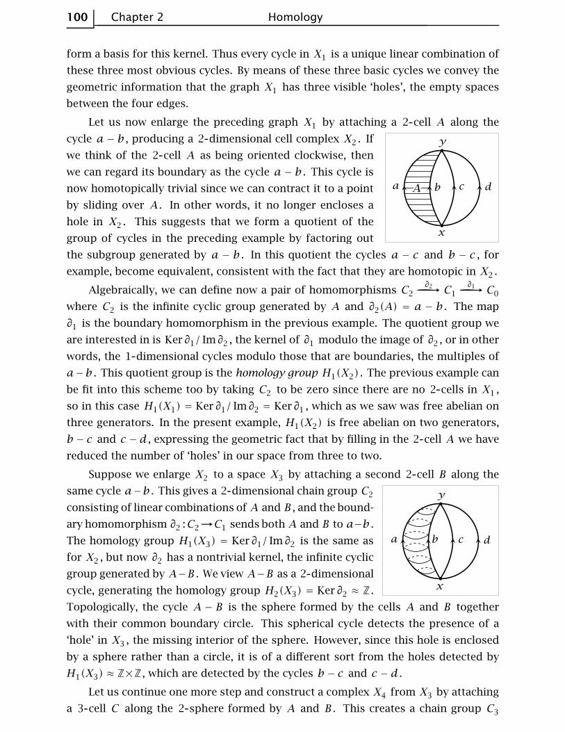
Let us now enlarge the preceding graph X1 by attaching a 2 cell A along the
cycle a − b , producing a 2 dimensional cell complex X2 . If
we think of the 2 cell A as being oriented clockwise, then
we can regard its boundary as the cycle a− b . This cycle is
now homotopically trivial since we can contract it to a point
by sliding over A . In other words, it no longer encloses a
hole in X2 . This suggests that we form a quotient of the
group of cycles in the preceding example by factoring out
the subgroup generated by a − b . In this quotient the cycles a − c and b − c , for
example, become equivalent, consistent with the fact that they are homotopic in X2 .
Algebraically, we can define now a pair of homomorphisms C2∂2------------→ C1
∂1------------→ C0
where C2 is the infinite cyclic group generated by A and ∂2(A) = a − b . The map
∂1 is the boundary homomorphism in the previous example. The quotient group we
are interested in is Ker ∂1/ Im∂2 , the kernel of ∂1 modulo the image of ∂2 , or in other
words, the 1 dimensional cycles modulo those that are boundaries, the multiples of
a−b . This quotient group is the homology group H1(X2) . The previous example can
be fit into this scheme too by taking C2 to be zero since there are no 2 cells in X1 ,
so in this case H1(X1) = Ker ∂1/ Im ∂2 = Ker ∂1 , which as we saw was free abelian on
three generators. In the present example, H1(X2) is free abelian on two generators,
b − c and c − d , expressing the geometric fact that by filling in the 2 cell A we have
reduced the number of ‘holes’ in our space from three to two.
Suppose we enlarge X2 to a space X3 by attaching a second 2 cell B along the
same cycle a−b . This gives a 2 dimensional chain group C2
consisting of linear combinations of A and B , and the bound-
ary homomorphism ∂2 :C2→C1 sends both A and B to a−b .
The homology group H1(X3) = Ker ∂1/ Im ∂2 is the same as
for X2 , but now ∂2 has a nontrivial kernel, the infinite cyclic
group generated by A−B . We view A−B as a 2 dimensional
cycle, generating the homology group H2(X3) = Ker ∂2 ≈ Z .
Topologically, the cycle A − B is the sphere formed by the cells A and B together
with their common boundary circle. This spherical cycle detects the presence of a
‘hole’ in X3 , the missing interior of the sphere. However, since this hole is enclosed
by a sphere rather than a circle, it is of a different sort from the holes detected by
H1(X3) ≈ Z×Z , which are detected by the cycles b − c and c − d .
Let us continue one more step and construct a complex X4 from X3 by attaching
a 3 cell C along the 2 sphere formed by A and B . This creates a chain group C3

The Idea of Homology 101
generated by this 3 cell C , and we define a boundary homomorphism ∂3 :C3→C2
sending C to A − B since the cycle A − B should be viewed as the boundary of C
in the same way that the 1 dimensional cycle a − b is the boundary of A . Now we
have a sequence of three boundary homomorphisms C3
∂3------------→C2∂2------------→C1
∂1------------→C0 and
the quotient H2(X4) = Ker ∂2/ Im ∂3 has become trivial. Also H3(X4) = Ker ∂3 = 0.
The group H1(X4) is the same as H1(X3) , namely Z×Z , so this is the only nontrivial
homology group of X4 .
It is clear what the general pattern of the examples is. For a cell complex X one
has chain groups Cn(X) which are free abelian groups with basis the n cells of X ,
and there are boundary homomorphisms ∂n :Cn(X)→Cn−1(X) , in terms of which
one defines the homology group Hn(X) = Ker ∂n/ Im∂n+1 . The major difficulty is
how to define ∂n in general. For n = 1 this is easy: The boundary of an oriented
edge is the vertex at its head minus the vertex at its tail. The next case n = 2 is also
not hard, at least for cells attached along cycles that are simply loops of edges, for
then the boundary of the cell is this cycle of edges, with the appropriate signs taking
orientations into account. But for larger n , matters become more complicated. Even
if one restricts attention to cell complexes formed from polyhedral cells with nice
attaching maps, there is still the matter of orientations to sort out.
The best solution to this problem seems to be to adopt an indirect approach.
Arbitrary polyhedra can always be subdivided into special polyhedra called simplices
(the triangle and the tetrahedron are the 2 dimensional and 3 dimensional instances)
so there is no loss of generality, though initially there is some loss of efficiency, in re-
stricting attention entirely to simplices. For simplices there is no difficulty in defining
boundary maps or in handling orientations. So one obtains a homology theory, called
simplicial homology, for cell complexes built from simplices. Still, this is a rather
restricted class of spaces, and the theory itself has a certain rigidity that makes it
awkward to work with.
The way around these obstacles is to step back from the geometry of spaces
decomposed into simplices and to consider instead something which at first glance
seems wildly more complicated, the collection of all possible continuous maps of
simplices into a given space X . These maps generate tremendously large chain groups
Cn(X) , but the quotients Hn(X) = Ker ∂n/ Im ∂n+1 , called singular homology groups,
turn out to be much smaller, at least for reasonably nice spaces X . In particular, for
spaces like those in the four examples above, the singular homology groups coincide
with the homology groups we computed from the cellular chains. And as we shall
see later in this chapter, singular homology allows one to define these nice cellular
homology groups for all cell complexes, and in particular to solve the problem of
defining the boundary maps for cellular chains.

102 Chapter 2 Homology
The most important homology theory in algebraic topology, and the one we shall
be studying almost exclusively, is called singular homology. Since the technical appa-
ratus of singular homology is somewhat complicated, we will first introduce a more
primitive version called simplicial homology in order to see how some of the apparatus
works in a simpler setting before beginning the general theory.
The natural domain of definition for simplicial homology is a class of spaces we
call ∆ complexes, which are a mild generalization of the more classical notion of
a simplicial complex. Historically, the modern definition of singular homology was
first given in [Eilenberg 1944], and ∆ complexes were introduced soon thereafter in
[Eilenberg-Zilber 1950] where they were called semisimplicial complexes. Within a
few years this term came to be applied to what Eilenberg and Zilber called complete
semisimplicial complexes, and later there was yet another shift in terminology as
the latter objects came to be called simplicial sets. In theory this frees up the term
semisimplicial complex to have its original meaning, but to avoid potential confusion
it seems best to introduce a new name, and the term ∆ complex has at least the virtue
of brevity.
D–Complexes
The torus, the projective plane, and the Klein bottle can each be obtained from a
square by identifying opposite edges in the way indicated by the arrows in the follow-
ing figures:
Cutting a square along a diagonal produces two triangles, so each of these surfaces
can also be built from two triangles by identifying their edges in pairs. In similar
fashion a polygon with any number of sides can be cut along
diagonals into triangles, so in fact all closed surfaces can be
constructed from triangles by identifying edges. Thus we have
a single building block, the triangle, from which all surfaces can
be constructed. Using only triangles we could also construct a
large class of 2 dimensional spaces that are not surfaces in the
strict sense, by allowing more than two edges to be identified
together at a time.

Simplicial and Singular Homology Section 2.1 103
The idea of a ∆ complex is to generalize constructions like these to any number
of dimensions. The n dimensional analog of the triangle is the n simplex. This is the
smallest convex set in a Euclidean space
Rm containing n + 1 points v0, ··· , vn
that do not lie in a hyperplane of dimen-
sion less than n , where by a hyperplane
we mean the set of solutions of a system
of linear equations. An equivalent condi-
tion would be that the difference vectors
v1 − v0, ··· , vn − v0 are linearly independent. The points vi are the vertices of the
simplex, and the simplex itself is denoted [v0, ··· , vn] . For exam-
ple, there is the standard n simplex
∆n = { (t0, ··· , tn) ∈ Rn+1 ||||∑iti = 1 and ti ≥ 0 for all i
}
whose vertices are the unit vectors along the coordinate axes.
For purposes of homology it will be important to keep track of the order of the
vertices of a simplex, so ‘n simplex’ will really mean ‘n simplex with an ordering
of its vertices’. A by-product of ordering the vertices of a simplex [v0, ··· , vn] is
that this determines orientations of the edges [vi, vj] according to increasing sub-
scripts, as shown in the two preceding figures. Specifying the ordering of the vertices
also determines a canonical linear homeomorphism from the standard n simplex
∆n onto any other n simplex [v0, ··· , vn] , preserving the order of vertices, namely,
(t0, ··· , tn)֏∑i tivi . The coefficients ti are the barycentric coordinates of the point∑
i tivi in [v0, ··· , vn] .
If we delete one of the n + 1 vertices of an n simplex [v0, ··· , vn] , then the
remaining n vertices span an (n − 1) simplex, called a face of [v0, ··· , vn] . We
adopt the following convention:
The vertices of a face, or of any subsimplex spanned by a subset of the vertices,
will always be ordered according to their order in the larger simplex.
The union of all the faces of ∆n is the boundary of ∆n , written ∂∆n . The open
simplex◦∆n is ∆n − ∂∆n , the interior of ∆n .
A D complex structure on a space X is a collection of maps σα :∆n→X , with n
depending on the index α , such that:
(i) The restriction σα ||◦∆n is injective, and each point of X is in the image of exactly
one such restriction σα ||◦∆n .
(ii) Each restriction of σα to a face of ∆n is one of the maps σβ :∆n−1→X . Here we
are identifying the face of ∆n with ∆n−1 by the canonical linear homeomorphism
between them that preserves the ordering of the vertices.
(iii) A set A ⊂ X is open iff σ−1α (A) is open in ∆n for each σα .

104 Chapter 2 Homology
Among other things, this last condition rules out trivialities like regarding all the
points of X as individual vertices. The earlier decompositions of the torus, projective
plane, and Klein bottle into two triangles, three edges, and one or two vertices define
∆ complex structures with a total of six σα ’s for the torus and Klein bottle and seven
for the projective plane. The orientations on the edges in the pictures are compatible
with a unique ordering of the vertices of each simplex, and these orderings determine
the maps σα .
A consequence of (iii) is that X can be built as a quotient space of a collection
of disjoint simplices ∆nα , one for each σα :∆n→X , the quotient space obtained by
identifying each face of a ∆nα with the ∆n−1β corresponding to the restriction σβ of
σα to the face in question, as in condition (ii). One can think of building the quotient
space inductively, starting with a discrete set of vertices, then attaching edges to
these to produce a graph, then attaching 2 simplices to the graph, and so on. From
this viewpoint we see that the data specifying a ∆ complex can be described purely
combinatorially as collections of n simplices ∆nα for each n together with functions
associating to each face of each n simplex ∆nα an (n− 1) simplex ∆n−1β .
More generally, ∆ complexes can be built from collections of disjoint simplices by
identifying various subsimplices spanned by subsets of the vertices, where the iden-
tifications are performed using the canonical linear homeomorphisms that preserve
the orderings of the vertices. The earlier ∆ complex structures on a torus, projective
plane, or Klein bottle can be obtained in this way, by identifying pairs of edges of
two 2 simplices. If one starts with a single 2 simplex and identifies all three edges
to a single edge, preserving the orientations given by the ordering of the vertices,
this produces a ∆ complex known as the ‘dunce hat’. By contrast, if the three edges
of a 2 simplex are identified preserving a cyclic orientation of the three edges, as in
the first figure at the right, this does not produce a
∆ complex structure, although if the 2 simplex is
subdivided into three smaller 2 simplices about a
central vertex, then one does obtain a ∆ complex
structure on the quotient space.
Thinking of a ∆ complex X as a quotient space of a collection of disjoint sim-
plices, it is not hard to see that X must be a Hausdorff space. Condition (iii) then
implies that each restriction σα ||◦∆n is a homeomorphism onto its image, which is
thus an open simplex in X . It follows from Proposition A.2 in the Appendix that
these open simplices σα(◦∆n) are the cells enα of a CW complex structure on X with
the σα ’s as characteristic maps. We will not need this fact at present, however.
Simplicial Homology
Our goal now is to define the simplicial homology groups of a ∆ complex X . Let
∆n(X) be the free abelian group with basis the open n simplices enα of X . Elements

Simplicial and Singular Homology Section 2.1 105
of ∆n(X) , called n chains, can be written as finite formal sums∑αnαe
nα with co-
efficients nα ∈ Z . Equivalently, we could write∑αnασα where σα :∆n→X is the
characteristic map of enα , with image the closure of enα as described above. Such a
sum∑αnασα can be thought of as a finite collection, or ‘chain’, of n simplices in X
with integer multiplicities, the coefficients nα .
As one can see in the next figure, the boundary of the n simplex [v0, ··· , vn] con-
sists of the various (n−1) dimensional simplices [v0, ··· , vi, ··· , vn] , where the ‘hat’
symbol over vi indicates that this vertex is deleted from the sequence v0, ··· , vn .
In terms of chains, we might then wish to say that the boundary of [v0, ··· , vn] is the
(n− 1) chain formed by the sum of the faces [v0, ··· , vi, ··· , vn] . However, it turns
out to be better to insert certain signs and instead let the boundary of [v0, ··· , vn] be∑i(−1)i[v0, ··· , vi, ··· , vn] . Heuristically, the signs are inserted to take orientations
into account, so that all the faces of a simplex are coherently oriented, as indicated in
the following figure:
∂[v0, v1] = [v1]− [v0]
∂[v0, v1, v2] = [v1, v2]− [v0, v2]+ [v0, v1]
∂[v0, v1, v2, v3] = [v1, v2, v3]− [v0, v2, v3]
+ [v0, v1, v3]− [v0, v1, v2]
In the last case, the orientations of the two hidden faces are also counterclockwise
when viewed from outside the 3 simplex.
With this geometry in mind we define for a general ∆ complex X a boundary
homomorphism ∂n :∆n(X)→∆n−1(X) by specifying its values on basis elements:
∂n(σα) =∑
i
(−1)iσα ||[v0, ··· , vi, ··· , vn]
Note that the right side of this equation does indeed lie in ∆n−1(X) since each restric-
tion σα ||[v0, ··· , vi, ··· , vn] is the characteristic map of an (n− 1) simplex of X .
Lemma 2.1. The composition ∆n(X)∂n------------→∆n−1(X)
∂n−1------------------→∆n−2(X) is zero.
Proof: We have ∂n(σ) =∑i(−1)iσ ||[v0, ··· , vi, ··· , vn] , and hence
∂n−1∂n(σ) =∑
j<i
(−1)i(−1)jσ ||[v0, ··· , vj , ··· , vi, ··· , vn]
+∑
j>i
(−1)i(−1)j−1σ ||[v0, ··· , vi, ··· , vj , ··· , vn]

106 Chapter 2 Homology
The latter two summations cancel since after switching i and j in the second sum, it
becomes the negative of the first. ⊔⊓
The algebraic situation we have now is a sequence of homomorphisms of abelian
groups
··· -→Cn+1∂n+1-----------------→Cn
∂n------------→Cn−1 -→··· -→C1∂1------------→C0
∂0------------→0
with ∂n∂n+1 = 0 for each n . Such a sequence is called a chain complex. Note that
we have extended the sequence by a 0 at the right end, with ∂0 = 0. The equation
∂n∂n+1 = 0 is equivalent to the inclusion Im ∂n+1 ⊂ Ker ∂n , where Im and Ker denote
image and kernel. So we can define the nth homology group of the chain complex to
be the quotient group Hn = Ker ∂n/ Im ∂n+1 . Elements of Ker ∂n are called cycles and
elements of Im ∂n+1 are called boundaries. Elements of Hn are cosets of Im ∂n+1 ,
called homology classes. Two cycles representing the same homology class are said
to be homologous. This means their difference is a boundary.
Returning to the case that Cn = ∆n(X) , the homology group Ker ∂n/ Im ∂n+1 will
be denoted H∆n(X) and called the nth simplicial homology group of X .
Example 2.2. X = S1 , with one vertex v and one edge e . Then ∆0(S1)
and ∆1(S1) are both Z and the boundary map ∂1 is zero since ∂e = v−v .
The groups ∆n(S1) are 0 for n ≥ 2 since there are no simplices in these
dimensions. Hence
H∆n(S1) ≈
{Z for n = 0,10 for n ≥ 2
This is an illustration of the general fact that if the boundary maps in a chain complex
are all zero, then the homology groups of the complex are isomorphic to the chain
groups themselves.
Example 2.3. X = T , the torus with the ∆ complex structure pictured earlier, having
one vertex, three edges a , b , and c , and two 2 simplices U and L . As in the previous
example, ∂1 = 0 so H∆0(T) ≈ Z . Since ∂2U = a+ b − c = ∂2L and {a,b,a+ b − c} is
a basis for ∆1(T) , it follows that H∆1 (T) ≈ Z⊕Z with basis the homology classes [a]
and [b] . Since there are no 3 simplices, H∆2 (T) is equal to Ker ∂2 , which is infinite
cyclic generated by U − L since ∂(pU + qL) = (p + q)(a+ b− c) = 0 only if p = −q .
Thus
H∆n(T) ≈
Z ⊕ Z for n = 1
Z for n = 0,20 for n ≥ 3
Example 2.4. X = RP2 , as pictured earlier, with two vertices v and w , three edges
a , b , and c , and two 2 simplices U and L . Then Im ∂1 is generated by w − v , so
H∆0 (X) ≈ Z with either vertex as a generator. Since ∂2U = −a+b+c and ∂2L = a−b+c ,
we see that ∂2 is injective, so H∆2 (X) = 0. Further, Ker ∂1 ≈ Z⊕Z with basis a−b and
c , and Im ∂2 is an index-two subgroup of Ker ∂1 since we can choose c and a−b+ c

Simplicial and Singular Homology Section 2.1 107
as a basis for Ker ∂1 and a− b+ c and 2c = (a− b+ c)+ (−a+ b+ c) as a basis for
Im ∂2 . Thus H∆1 (X) ≈ Z2 .
Example 2.5. We can obtain a ∆ complex structure on Sn by taking two copies of ∆nand identifying their boundaries via the identity map. Labeling these two n simplices
U and L , then it is obvious that Ker ∂n is infinite cyclic generated by U − L . Thus
H∆n(Sn) ≈ Z for this ∆ complex structure on Sn . Computing the other homology
groups would be more difficult.
Many similar examples could be worked out without much trouble, such as the
other closed orientable and nonorientable surfaces. However, the calculations do tend
to increase in complexity before long, particularly for higher-dimensional complexes.
Some obvious general questions arise: Are the groups H∆n(X) independent of
the choice of ∆ complex structure on X ? In other words, if two ∆ complexes are
homeomorphic, do they have isomorphic homology groups? More generally, do they
have isomorphic homology groups if they are merely homotopy equivalent? To answer
such questions and to develop a general theory it is best to leave the rather rigid
simplicial realm and introduce the singular homology groups. These have the added
advantage that they are defined for all spaces, not just ∆ complexes. At the end of
this section, after some theory has been developed, we will show that simplicial and
singular homology groups coincide for ∆ complexes.
Traditionally, simplicial homology is defined for simplicial complexes, which are
the ∆ complexes whose simplices are uniquely determined by their vertices. This
amounts to saying that each n simplex has n+ 1 distinct vertices, and that no other
n simplex has this same set of vertices. Thus a simplicial complex can be described
combinatorially as a set X0 of vertices together with sets Xn of n simplices, which
are (n+1) element subsets of X0 . The only requirement is that each (k+1) element
subset of the vertices of an n simplex in Xn is a k simplex, in Xk . From this combi-
natorial data a ∆ complex X can be constructed, once we choose a partial ordering
of the vertices X0 that restricts to a linear ordering on the vertices of each simplex
in Xn . For example, we could just choose a linear ordering of all the vertices. This
might perhaps involve invoking the Axiom of Choice for large vertex sets.
An exercise at the end of this section is to show that every ∆ complex can be
subdivided to be a simplicial complex. In particular, every ∆ complex is then homeo-
morphic to a simplicial complex.
Compared with simplicial complexes, ∆ complexes have the advantage of simpler
computations since fewer simplices are required. For example, to put a simplicial
complex structure on the torus one needs at least 14 triangles, 21 edges, and 7 vertices,
and for RP2 one needs at least 10 triangles, 15 edges, and 6 vertices. This would slow
down calculations considerably!

108 Chapter 2 Homology
Singular Homology
A singular n simplex in a space X is by definition just a map σ :∆n→X . The
word ‘singular’ is used here to express the idea that σ need not be a nice embedding
but can have ‘singularities’ where its image does not look at all like a simplex. All that
is required is that σ be continuous. Let Cn(X) be the free abelian group with basis
the set of singular n simplices in X . Elements of Cn(X) , called n chains, or more
precisely singularn chains, are finite formal sums∑iniσi for ni ∈ Z and σi :∆n→X .
A boundary map ∂n :Cn(X)→Cn−1(X) is defined by the same formula as before:
∂n(σ) =∑
i
(−1)iσ ||[v0, ··· , vi, ··· , vn]
Implicit in this formula is the canonical identification of [v0, ··· , vi, ··· , vn] with
∆n−1 , preserving the ordering of vertices, so that σ ||[v0, ··· , vi, ··· , vn] is regarded
as a map ∆n−1→X , that is, a singular (n− 1) simplex.
Often we write the boundary map ∂n from Cn(X) to Cn−1(X) simply as ∂ when
this does not lead to serious ambiguities. The proof of Lemma 2.1 applies equally well
to singular simplices, showing that ∂n∂n+1 = 0 or more concisely ∂2= 0, so we can
define the singular homology group Hn(X) = Ker ∂n/ Im∂n+1 .
It is evident from the definition that homeomorphic spaces have isomorphic sin-
gular homology groups Hn , in contrast with the situation for H∆n . On the other hand,
since the groups Cn(X) are so large, the number of singular n simplices in X usually
being uncountable, it is not at all clear that for a ∆ complex X with finitely many sim-
plices, Hn(X) should be finitely generated for all n , or that Hn(X) should be zero
for n larger than the dimension of X — two properties that are trivial for H∆n(X) .
Though singular homology looks so much more general than simplicial homology,
it can actually be regarded as a special case of simplicial homology by means of the
following construction. For an arbitrary space X , define the singular complex S(X)
to be the ∆ complex with one n simplex ∆nσ for each singular n simplex σ :∆n→X ,
with ∆nσ attached in the obvious way to the (n − 1) simplices of S(X) that are the
restrictions of σ to the various (n− 1) simplices in ∂∆n . It is clear from the defini-
tions that H∆n(S(X)
)is identical with Hn(X) for all n , and in this sense the singular
homology group Hn(X) is a special case of a simplicial homology group. One can
regard S(X) as a ∆ complex model for X , although it is usually an extremely large
object compared to X .
Cycles in singular homology are defined algebraically, but they can be given a
somewhat more geometric interpretation in terms of maps from finite ∆ complexes.
To see this, note first that a singular n chain ξ can always be written in the form∑i εiσi with εi = ±1, allowing repetitions of the singular n simplices σi . Given such
an n chain ξ =∑i εiσi , when we compute ∂ξ as a sum of singular (n−1) simplices
with signs ±1, there may be some canceling pairs consisting of two identical singu-
lar (n − 1) simplices with opposite signs. Choosing a maximal collection of such

Simplicial and Singular Homology Section 2.1 109
canceling pairs, construct an n dimensional ∆ complex Kξ from a disjoint union of
n simplices ∆ni , one for each σi , by identifying the pairs of (n−1) dimensional faces
corresponding to the chosen canceling pairs. The σi ’s then induce a map Kξ→X . If
ξ is a cycle, all the (n−1) dimensional faces of the ∆ni ’s are identified in pairs. Thus
Kξ is a manifold, locally homeomorphic to Rn , near all points in the complement
of the (n − 2) skeleton Kn−2ξ of Kξ . All the n simplices of Kξ can be coherently
oriented by taking the signs of the σi ’s into account, so Kξ − Kn−2ξ is actually an
oriented manifold. A closer inspection shows that Kξ is also a manifold near points
in the interiors of (n − 2) simplices, so the nonmanifold points of Kξ in fact lie in
the (n−3) skeleton. However, near points in the interiors of (n−3) simplices it can
very well happen that Kξ is not a manifold.
In particular, elements of H1(X) are represented by collections of oriented loops
in X , and elements of H2(X) are represented by maps of closed oriented surfaces
into X . With a bit more work it can be shown that an oriented 1 cycle∐αS
1α→X is
zero in H1(X) iff it extends to a map of a compact oriented surface with boundary∐αS
1α into X . The analogous statement for 2 cycles is also true. In the early days of
homology theory it may have been believed, or at least hoped, that this close connec-
tion with manifolds continued in all higher dimensions, but this has turned out not to
be the case. There is a sort of homology theory built from manifolds, called bordism,
but it is quite a bit more complicated than the homology theory we are studying here.
After these preliminary remarks let us begin to see what can be proved about
singular homology.
Proposition 2.6. Corresponding to the decomposition of a space X into its path-
components Xα there is an isomorphism of Hn(X) with the direct sum⊕αHn(Xα) .
Proof: Since a singular simplex always has path-connected image, Cn(X) splits as the
direct sum of its subgroups Cn(Xα) . The boundary maps ∂n preserve this direct sum
decomposition, taking Cn(Xα) to Cn−1(Xα) , so Ker ∂n and Im ∂n+1 split similarly as
direct sums, hence the homology groups also split, Hn(X) ≈⊕αHn(Xα) . ⊔⊓
Proposition 2.7. If X is nonempty and path-connected, then H0(X) ≈ Z . Hence for
any space X , H0(X) is a direct sum of Z ’s, one for each path-component of X .
Proof: By definition, H0(X) = C0(X)/ Im ∂1 since ∂0 = 0. Define a homomorphism
ε :C0(X)→Z by ε(∑
iniσi)=∑ini . This is obviously surjective if X is nonempty.
The claim is that Ker ε = Im ∂1 if X is path-connected, and hence ε induces an iso-
morphism H0(X) ≈ Z .
To verify the claim, observe first that Im ∂1 ⊂ Ker ε since for a singular 1 simplex
σ :∆1→X we have ε∂1(σ) = ε(σ ||[v1] − σ ||[v0]
)= 1 − 1 = 0. For the reverse
inclusion Ker ε ⊂ Im ∂1 , suppose ε(∑
iniσi)= 0, so
∑ini = 0. The σi ’s are singular
0 simplices, which are simply points of X . Choose a path τi : I→X from a basepoint

110 Chapter 2 Homology
x0 to σi(v0) and let σ0 be the singular 0 simplex with image x0 . We can view τias a singular 1 simplex, a map τi : [v0, v1]→X , and then we have ∂τi = σi − σ0 .
Hence ∂(∑
iniτi)=∑iniσi −
∑iniσ0 =
∑iniσi since
∑ini = 0. Thus
∑iniσi is a
boundary, which shows that Ker ε ⊂ Im ∂1 . ⊔⊓
Proposition 2.8. If X is a point, then Hn(X) = 0 for n > 0 and H0(X) ≈ Z .
Proof: In this case there is a unique singular n simplex σn for each n , and ∂(σn) =∑i(−1)iσn−1 , a sum of n+ 1 terms, which is therefore 0 for n odd and σn−1 for n
even, n ≠ 0. Thus we have the chain complex
··· -→Z≈------------→Z
0------------→Z
≈------------→Z
0------------→Z -→0
with boundary maps alternately isomorphisms and trivial maps, except at the last Z .
The homology groups of this complex are trivial except for H0 ≈ Z . ⊔⊓
It is often very convenient to have a slightly modified version of homology for
which a point has trivial homology groups in all dimensions, including zero. This is
done by defining the reduced homology groups Hn(X) to be the homology groups
of the augmented chain complex
··· -→C2(X)∂2------------→C1(X)
∂1------------→C0(X)ε------------→Z -→0
where ε(∑
iniσi)=∑ini as in the proof of Proposition 2.7. Here we had better
require X to be nonempty, to avoid having a nontrivial homology group in dimension
−1. Since ε∂1 = 0, ε vanishes on Im ∂1 and hence induces a map H0(X)→Z with
kernel H0(X) , so H0(X) ≈ H0(X)⊕Z . Obviously Hn(X) ≈ Hn(X) for n > 0.
Formally, one can think of the extra Z in the augmented chain complex as gener-
ated by the unique map [∅]→X where [∅] is the empty simplex, with no vertices.
The augmentation map ε is then the usual boundary map since ∂[v0] = [v0] = [∅] .
Readers who know about the fundamental group π1(X) may wish to make a
detour here to look at §2.A where it is shown that H1(X) is the abelianization of
π1(X) whenever X is path-connected. This result will not be needed elsewhere in the
chapter, however.
Homotopy Invariance
The first substantial result we will prove about singular homology is that ho-
motopy equivalent spaces have isomorphic homology groups. This will be done by
showing that a map f :X→Y induces a homomorphism f∗ :Hn(X)→Hn(Y ) for each
n , and that f∗ is an isomorphism if f is a homotopy equivalence.
For a map f :X→Y , an induced homomorphism f♯ :Cn(X)→Cn(Y ) is defined
by composing each singular n simplex σ :∆n→X with f to get a singular n simplex

Simplicial and Singular Homology Section 2.1 111
f♯(σ) = fσ :∆n→Y , then extending f♯ linearly via f♯(∑
iniσi)=∑inif♯(σi) =∑
inifσi . The maps f♯ :Cn(X)→Cn(Y ) satisfy f♯∂ = ∂f♯ since
f♯∂(σ) = f♯(∑
i(−1)iσ ||[v0, ··· , vi, ··· , vn])
=∑i(−1)ifσ ||[v0, ··· , vi, ··· , vn] = ∂f♯(σ)
Thus we have a diagram
such that in each square the composition f♯∂ equals the composition ∂f♯ . A diagram
of maps with the property that any two compositions of maps starting at one point in
the diagram and ending at another are equal is called a commutative diagram. In the
present case commutativity of the diagram is equivalent to the commutativity relation
f♯∂ = ∂f♯ , but commutative diagrams can contain commutative triangles, pentagons,
etc., as well as commutative squares.
The fact that the maps f♯ :Cn(X)→Cn(Y ) satisfy f♯∂ = ∂f♯ is also expressed
by saying that the f♯ ’s define a chain map from the singular chain complex of X
to that of Y . The relation f♯∂ = ∂f♯ implies that f♯ takes cycles to cycles since
∂α = 0 implies ∂(f♯α) = f♯(∂α) = 0. Also, f♯ takes boundaries to boundaries
since f♯(∂β) = ∂(f♯β) . Hence f♯ induces a homomorphism f∗ :Hn(X)→Hn(Y ) . An
algebraic statement of what we have just proved is:
Proposition 2.9. A chain map between chain complexes induces homomorphisms
between the homology groups of the two complexes. ⊔⊓
Two basic properties of induced homomorphisms which are important in spite
of being rather trivial are:
(i) (fg)∗ = f∗g∗ for a composed mapping Xg-----→ Y
f-----→ Z . This follows from
associativity of compositions ∆n σ-----→X
g-----→Y
f-----→Z .
(ii) 11∗ = 11 where 11 denotes the identity map of a space or a group.
Less trivially, we have:
Theorem 2.10. If two maps f ,g :X→Y are homotopic, then they induce the same
homomorphism f∗ = g∗ :Hn(X)→Hn(Y ) .
In view of the formal properties (fg)∗ = f∗g∗ and 11∗ = 11, this immediately
implies:
Corollary 2.11. The maps f∗ :Hn(X)→Hn(Y ) induced by a homotopy equivalence
f :X→Y are isomorphisms for all n . ⊔⊓
For example, if X is contractible then Hn(X) = 0 for all n .

112 Chapter 2 Homology
Proof of 2.10: The essential ingredient is a procedure for
subdividing ∆n×I into simplices. The figure shows the
cases n = 1,2. In ∆n×I , let ∆n×{0} = [v0, ··· , vn]
and ∆n×{1} = [w0, ··· ,wn] , where vi and wi have the
same image under the projection ∆n×I→∆n . We can pass
from [v0, ··· , vn] to [w0, ··· ,wn] by interpolating a se-
quence of n simplices, each obtained from the preceding
one by moving one vertex vi up to wi , starting with vnand working backwards to v0 . Thus the first step is to
move [v0, ··· , vn] up to [v0, ··· , vn−1,wn] , then the sec-
ond step is to move this up to [v0, ··· , vn−2,wn−1,wn] ,
and so on. In the typical step [v0, ··· , vi,wi+1, ··· ,wn]
moves up to [v0, ··· , vi−1,wi, ··· ,wn] . The region be-
tween these two n simplices is exactly the (n+1) simplex
[v0, ··· , vi,wi, ··· ,wn] which has [v0, ··· , vi,wi+1, ··· ,wn] as its lower face and
[v0, ··· , vi−1,wi, ··· ,wn] as its upper face. Altogether, ∆n×I is the union of the
(n+1) simplices [v0, ··· , vi,wi, ··· ,wn] , each intersecting the next in an n simplex
face.
Given a homotopy F :X×I→Y from f to g and a singular simplex σ :∆n→X ,
we can form the composition F ◦ (σ×11) :∆n×I→X×I→Y . Using this, we can define
prism operators P :Cn(X)→Cn+1(Y ) by the following formula:
P(σ) =∑
i
(−1)iF ◦ (σ×11)||[v0, ··· , vi,wi, ··· ,wn]
We will show that these prism operators satisfy the basic relation
∂P = g♯ − f♯ − P∂
Geometrically, the left side of this equation represents the boundary of the prism, and
the three terms on the right side represent the top ∆n×{1} , the bottom ∆n×{0} , and
the sides ∂∆n×I of the prism. To prove the relation we calculate
∂P(σ) =∑
j≤i
(−1)i(−1)jF◦(σ×11)||[v0, ··· , vj , ··· , vi,wi, ··· ,wn]
+∑
j≥i
(−1)i(−1)j+1F◦(σ×11)||[v0, ··· , vi,wi, ··· , wj , ··· ,wn]
The terms with i = j in the two sums cancel except for F ◦ (σ×11)||[v0,w0, ··· ,wn] ,
which is g ◦σ = g♯(σ) , and −F ◦ (σ×11)||[v0, ··· , vn, wn] , which is −f ◦σ = −f♯(σ) .
The terms with i ≠ j are exactly −P∂(σ) since
P∂(σ) =∑
i<j
(−1)i(−1)jF◦(σ×11)||[v0, ··· , vi,wi, ··· , wj , ··· ,wn]
+∑
i>j
(−1)i−1(−1)jF◦(σ×11)||[v0, ··· , vj , ··· , vi,wi, ··· ,wn]

Simplicial and Singular Homology Section 2.1 113
Now we can finish the proof of the theorem. If α ∈ Cn(X) is a cycle, then we
have g♯(α)− f♯(α) = ∂P(α)+ P∂(α) = ∂P(α) since ∂α = 0. Thus g♯(α)− f♯(α) is
a boundary, so g♯(α) and f♯(α) determine the same homology class, which means
that g∗ equals f∗ on the homology class of α . ⊔⊓
The relationship ∂P+P∂ = g♯−f♯ is expressed by saying P is a chain homotopy
between the chain maps f♯ and g♯ . We have just shown:
Proposition 2.12. Chain-homotopic chain maps induce the same homomorphism on
homology. ⊔⊓
There are also induced homomorphisms f∗ : Hn(X)→Hn(Y ) for reduced homol-
ogy groups since f♯ε = εf♯ where f♯ is the identity map on the added groups Z in the
augmented chain complexes. The properties of induced homomorphisms we proved
above hold equally well in the setting of reduced homology, with the same proofs.
Exact Sequences and Excision
If there was always a simple relationship between the homology groups of a space
X , a subspace A , and the quotient space X/A , then this could be a very useful tool
in understanding the homology groups of spaces such as CW complexes that can be
built inductively from successively more complicated subspaces. Perhaps the simplest
possible relationship would be if Hn(X) contained Hn(A) as a subgroup and the
quotient group Hn(X)/Hn(A) was isomorphic to Hn(X/A) . While this does hold
in some cases, if it held in general then homology theory would collapse totally since
every space X can be embedded as a subspace of a space with trivial homology groups,
namely the cone CX = (X×I)/(X×{0}) , which is contractible.
It turns out that this overly simple model does not have to be modified too much
to get a relationship that is valid in fair generality. The novel feature of the actual
relationship is that it involves the groups Hn(X) , Hn(A) , and Hn(X/A) for all values
of n simultaneously. In practice this is not as bad as it might sound, and in addition
it has the pleasant side effect of sometimes allowing higher-dimensional homology
groups to be computed in terms of lower-dimensional groups which may already be
known, for example by induction.
In order to formulate the relationship we are looking for, we need an algebraic
definition which is central to algebraic topology. A sequence of homomorphisms
··· ---------→An+1αn+1-------------------------→An
αn------------------→An−1 ---------→ ···
is said to be exact if Kerαn = Imαn+1 for each n . The inclusions Imαn+1 ⊂ Kerαnare equivalent to αnαn+1 = 0, so the sequence is a chain complex, and the opposite
inclusions Kerαn ⊂ Imαn+1 say that the homology groups of this chain complex are
trivial.

114 Chapter 2 Homology
A number of basic algebraic concepts can be expressed in terms of exact se-
quences, for example:
(i) 0 -→Aα-----→B is exact iff Kerα = 0, i.e., α is injective.
(ii) Aα-----→B -→0 is exact iff Imα = B , i.e., α is surjective.
(iii) 0 -→Aα-----→B -→0 is exact iff α is an isomorphism, by (i) and (ii).
(iv) 0 -→Aα-----→ B
β-----→ C -→ 0 is exact iff α is injective, β is surjective, and Kerβ =
Imα , so β induces an isomorphism C ≈ B/ Imα . This can be written C ≈ B/A if
we think of α as an inclusion of A as a subgroup of B .
An exact sequence 0→A→B→C→0 as in (iv) is called a short exact sequence.
Exact sequences provide the right tool to relate the homology groups of a space,
a subspace, and the associated quotient space:
Theorem 2.13. If X is a space and A is a nonempty closed subspace that is a defor-
mation retract of some neighborhood in X , then there is an exact sequence
··· -----→Hn(A)i∗------------→ Hn(X)
j∗------------→ Hn(X/A)
∂-----→Hn−1(A)
i∗------------→ Hn−1(X) -----→···
··· -----→H0(X/A) -----→0
where i is the inclusion AX and j is the quotient map X→X/A .
The map ∂ will be constructed in the course of the proof. The idea is that an
element x ∈ Hn(X/A) can be represented by a chain α in X with ∂α a cycle in A
whose homology class is ∂x ∈ Hn−1(A) .
Pairs of spaces (X,A) satisfying the hypothesis of the theorem will be called
good pairs. For example, if X is a CW complex and A is a nonempty subcomplex,
then (X,A) is a good pair by Proposition A.5 in the Appendix.
Corollary 2.14. Hn(Sn) ≈ Z and Hi(S
n) = 0 for i ≠ n .
Proof: For n > 0 take (X,A) = (Dn, Sn−1) so X/A = Sn . The terms Hi(Dn) in the
long exact sequence for this pair are zero since Dn is contractible. Exactness of the
sequence then implies that the maps Hi(Sn)
∂-----→ Hi−1(S
n−1) are isomorphisms for
i > 0 and that H0(Sn) = 0. The result now follows by induction on n , starting with
the case of S0 where the result holds by Propositions 2.6 and 2.8. ⊔⊓
As an application of this calculation we have the following classical theorem of
Brouwer, the 2 dimensional case of which was proved in §1.1.
Corollary 2.15. ∂Dn is not a retract of Dn . Hence every map f :Dn→Dn has a
fixed point.
Proof: If r :Dn→∂Dn is a retraction, then ri = 11 for i : ∂Dn→Dn the inclusion map.
The composition Hn−1(∂Dn)
i∗------------→ Hn−1(Dn)
r∗------------→ Hn−1(∂Dn) is then the identity map

Simplicial and Singular Homology Section 2.1 115
on Hn−1(∂Dn) ≈ Z . But i∗ and r∗ are both 0 since Hn−1(D
n) = 0, and we have a
contradiction. The statement about fixed points follows as in Theorem 1.9. ⊔⊓
The derivation of the exact sequence of homology groups for a good pair (X,A)
will be rather a long story. We will in fact derive a more general exact sequence which
holds for arbitrary pairs (X,A) , but with the homology groups of the quotient space
X/A replaced by relative homology groups, denoted Hn(X,A) . These turn out to be
quite useful for many other purposes as well.
Relative Homology Groups
It sometimes happens that by ignoring a certain amount of data or structure one
obtains a simpler, more flexible theory which, almost paradoxically, can give results
not readily obtainable in the original setting. A familiar instance of this is arithmetic
mod n , where one ignores multiples of n . Relative homology is another example. In
this case what one ignores is all singular chains in a subspace of the given space.
Relative homology groups are defined in the following way. Given a space X and
a subspace A ⊂ X , let Cn(X,A) be the quotient group Cn(X)/Cn(A) . Thus chains in
A are trivial in Cn(X,A) . Since the boundary map ∂ :Cn(X)→Cn−1(X) takes Cn(A)
to Cn−1(A) , it induces a quotient boundary map ∂ :Cn(X,A)→Cn−1(X,A) . Letting n
vary, we have a sequence of boundary maps
··· -→Cn(X,A)∂------------→Cn−1(X,A) -→···
The relation ∂2= 0 holds for these boundary maps since it holds before passing to
quotient groups. So we have a chain complex, and the homology groups Ker ∂/ Im∂
of this chain complex are by definition the relative homology groups Hn(X,A) . By
considering the definition of the relative boundary map we see:
Elements of Hn(X,A) are represented by relative cycles: n chains α ∈ Cn(X)
such that ∂α ∈ Cn−1(A) .
A relative cycle α is trivial in Hn(X,A) iff it is a relative boundary: α = ∂β+ γ
for some β ∈ Cn+1(X) and γ ∈ Cn(A) .
These properties make precise the intuitive idea that Hn(X,A) is ‘homology of X
modulo A ’.
The quotient Cn(X)/Cn(A) could also be viewed as a subgroup of Cn(X) , the
subgroup with basis the singular n simplices σ :∆n→X whose image is not con-
tained in A . However, the boundary map does not take this subgroup of Cn(X) to
the corresponding subgroup of Cn−1(X) , so it is usually better to regard Cn(X,A) as
a quotient rather than a subgroup of Cn(X) .
Our goal now is to show that the relative homology groups Hn(X,A) for any pair
(X,A) fit into a long exact sequence
··· -→Hn(A) -→Hn(X) -→Hn(X,A) -→Hn−1(A) -→Hn−1(X) -→···
··· -→H0(X,A) -→0

116 Chapter 2 Homology
This will be entirely a matter of algebra. To start the process, consider the diagram
where i is inclusion and j is the quotient map. The diagram is commutative by the def-
inition of the boundary maps. Letting n vary, and drawing these short exact sequences
vertically rather than horizontally, we
have a large commutative diagram of
the form shown at the right, where the
columns are exact and the rows are
chain complexes which we denote A ,
B , and C . Such a diagram is called a
short exact sequence of chain com-
plexes. We will show that when we
pass to homology groups, this short
exact sequence of chain complexes stretches out into a long exact sequence of homol-
ogy groups
··· -→Hn(A)i∗------------→Hn(B)
j∗------------→Hn(C)
∂-----→Hn−1(A)
i∗------------→Hn−1(B) -→···
where Hn(A) denotes the homology group Ker ∂/ Im∂ at An in the chain complex A ,
and Hn(B) and Hn(C) are defined similarly.
The commutativity of the squares in the short exact sequence of chain complexes
means that i and j are chain maps. These therefore induce maps i∗ and j∗ on
homology. To define the boundary map ∂ :Hn(C)→Hn−1(A) , let c ∈ Cn be a cycle.
Since j is onto, c = j(b) for some b ∈ Bn . The element ∂b ∈ Bn−1
is in Ker j since j(∂b) = ∂j(b) = ∂c = 0. So ∂b = i(a) for some
a ∈ An−1 since Ker j = Im i . Note that ∂a = 0 since i(∂a) =
∂i(a) = ∂∂b = 0 and i is injective. We define ∂ :Hn(C)→Hn−1(A)
by sending the homology class of c to the homology class of a ,
∂[c] = [a] . This is well-defined since:
The element a is uniquely determined by ∂b since i is injective.
A different choice b′ for b would have j(b′) = j(b) , so b′ −b is in Ker j = Im i .
Thus b′ − b = i(a′) for some a′ , hence b′ = b + i(a′) . The effect of replacing b
by b+i(a′) is to change a to the homologous element a+∂a′ since i(a+∂a′) =
i(a)+ i(∂a′) = ∂b + ∂i(a′) = ∂(b + i(a′)) .
A different choice of c within its homology class would have the form c + ∂c′ .
Since c′ = j(b′) for some b′ , we then have c + ∂c′ = c + ∂j(b′) = c + j(∂b′) =
j(b + ∂b′) , so b is replaced by b + ∂b′ , which leaves ∂b and therefore also a
unchanged.

Simplicial and Singular Homology Section 2.1 117
The map ∂ :Hn(C)→Hn−1(A) is a homomorphism since if ∂[c1] = [a1] and ∂[c2] =
[a2] via elements b1 and b2 as above, then j(b1 + b2) = j(b1)+ j(b2) = c1 + c2 and
i(a1 + a2) = i(a1)+ i(a2) = ∂b1 + ∂b2 = ∂(b1 + b2) , so ∂([c1]+ [c2]) = [a1]+ [a2] .
Theorem 2.16. The sequence of homology groups
··· -→Hn(A)i∗------------→Hn(B)
j∗------------→Hn(C)
∂-----→Hn−1(A)
i∗------------→Hn−1(B) -→···is exact.
Proof: There are six things to verify:
Im i∗ ⊂ Ker j∗ . This is immediate since ji = 0 implies j∗i∗ = 0.
Im j∗ ⊂ Ker ∂ . We have ∂j∗ = 0 since in this case ∂b = 0 in the definition of ∂ .
Im ∂ ⊂ Ker i∗ . Here i∗∂ = 0 since i∗∂ takes [c] to [∂b] = 0.
Ker j∗ ⊂ Im i∗ . A homology class in Ker j∗ is represented by a cycle b ∈ Bn with
j(b) a boundary, so j(b) = ∂c′ for some c′ ∈ Cn+1 . Since j is surjective, c′ = j(b′)
for some b′ ∈ Bn+1 . We have j(b − ∂b′) = j(b) − j(∂b′) = j(b) − ∂j(b′) = 0 since
∂j(b′) = ∂c′ = j(b) . So b − ∂b′ = i(a) for some a ∈ An . This a is a cycle since
i(∂a) = ∂i(a) = ∂(b−∂b′) = ∂b = 0 and i is injective. Thus i∗[a] = [b−∂b′] = [b] ,
showing that i∗ maps onto Ker j∗ .
Ker ∂ ⊂ Im j∗ . In the notation used in the definition of ∂ , if c represents a homology
class in Ker ∂ , then a = ∂a′ for some a′ ∈ An . The element b − i(a′) is a cycle
since ∂(b − i(a′)) = ∂b − ∂i(a′) = ∂b − i(∂a′) = ∂b − i(a) = 0. And j(b − i(a′)) =
j(b) − ji(a′) = j(b) = c , so j∗ maps [b − i(a′)] to [c] .
Ker i∗ ⊂ Im ∂ . Given a cycle a ∈ An−1 such that i(a) = ∂b for some b ∈ Bn , then
j(b) is a cycle since ∂j(b) = j(∂b) = ji(a) = 0, and ∂ takes [j(b)] to [a] . ⊔⊓
This theorem represents the beginnings of the subject of homological algebra.
The method of proof is sometimes called diagram chasing.
Returning to topology, the preceding algebraic theorem yields a long exact se-
quence of homology groups:
··· -→Hn(A)i∗------------→Hn(X)
j∗------------→Hn(X,A)
∂-----→Hn−1(A)
i∗------------→Hn−1(X) -→···
··· -→H0(X,A) -→0
The boundary map ∂ :Hn(X,A)→Hn−1(A) has a very simple description: If a class
[α] ∈ Hn(X,A) is represented by a relative cycle α , then ∂[α] is the class of the
cycle ∂α in Hn−1(A) . This is immediate from the algebraic definition of the boundary
homomorphism in the long exact sequence of homology groups associated to a short
exact sequence of chain complexes.
This long exact sequence makes precise the idea that the groups Hn(X,A) mea-
sure the difference between the groups Hn(X) and Hn(A) . In particular, exactness

118 Chapter 2 Homology
implies that if Hn(X,A) = 0 for all n , then the inclusion AX induces isomorphisms
Hn(A) ≈ Hn(X) for all n , by the remark (iii) following the definition of exactness. The
converse is also true according to an exercise at the end of this section.
There is a completely analogous long exact sequence of reduced homology groups
for a pair (X,A) with A ≠∅ . This comes from applying the preceding algebraic ma-
chinery to the short exact sequence of chain complexes formed by the short exact se-
quences 0→Cn(A)→Cn(X)→Cn(X,A)→0 in nonnegative dimensions, augmented
by the short exact sequence 0 -→Z11-----→ Z -→ 0 -→ 0 in dimension −1. In particular
this means that Hn(X,A) is the same as Hn(X,A) for all n , when A ≠∅ .
Example 2.17. In the long exact sequence of reduced homology groups for the pair
(Dn, ∂Dn) , the maps Hi(Dn, ∂Dn)
∂-----→ Hi−1(S
n−1) are isomorphisms for all i > 0
since the remaining terms Hi(Dn) are zero for all i . Thus we obtain the calculation
Hi(Dn, ∂Dn) ≈
{Z for i = n0 otherwise
Example 2.18. Applying the long exact sequence of reduced homology groups to a
pair (X,x0) with x0 ∈ X yields isomorphisms Hn(X,x0) ≈ Hn(X) for all n since
Hn(x0) = 0 for all n .
There are induced homomorphisms for relative homology just as there are in the
nonrelative, or ‘absolute’, case. A map f :X→Y with f(A) ⊂ B , or more concisely
f : (X,A)→(Y , B) , induces homomorphisms f♯ :Cn(X,A)→Cn(Y , B) since the chain
map f♯ :Cn(X)→Cn(Y ) takes Cn(A) to Cn(B) , so we get a well-defined map on quo-
tients, f♯ :Cn(X,A)→Cn(Y , B) . The relation f♯∂ = ∂f♯ holds for relative chains since
it holds for absolute chains. By Proposition 2.9 we then have induced homomorphisms
f∗ :Hn(X,A)→Hn(Y , B) .
Proposition 2.19. If two maps f ,g : (X,A)→(Y , B) are homotopic through maps of
pairs (X,A)→(Y , B) , then f∗ = g∗ :Hn(X,A)→Hn(Y , B) .
Proof: The prism operator P from the proof of Theorem 2.10 takes Cn(A) to Cn+1(B) ,
hence induces a relative prism operator P :Cn(X,A)→Cn+1(Y , B) . Since we are just
passing to quotient groups, the formula ∂P + P∂ = g♯ − f♯ remains valid. Thus the
maps f♯ and g♯ on relative chain groups are chain homotopic, and hence they induce
the same homomorphism on relative homology groups. ⊔⊓
An easy generalization of the long exact sequence of a pair (X,A) is the long
exact sequence of a triple (X,A, B) , where B ⊂ A ⊂ X :
··· -→Hn(A, B) -→Hn(X, B) -→Hn(X,A) -→Hn−1(A, B) -→···
This is the long exact sequence of homology groups associated to the short exact
sequence of chain complexes formed by the short exact sequences
0 -→Cn(A, B) -→Cn(X, B) -→Cn(X,A) -→0

Simplicial and Singular Homology Section 2.1 119
For example, taking B to be a point, the long exact sequence of the triple (X,A, B)
becomes the long exact sequence of reduced homology for the pair (X,A) .
Excision
A fundamental property of relative homology groups is given by the following
Excision Theorem, describing when the relative groups Hn(X,A) are unaffected by
deleting, or excising, a subset Z ⊂ A .
Theorem 2.20. Given subspaces Z ⊂ A ⊂ X such that the closure of Z is contained
in the interior of A , then the inclusion (X − Z,A − Z) (X,A) induces isomor-
phisms Hn(X−Z,A−Z)→Hn(X,A) for all n . Equivalently, for subspaces A,B ⊂ X
whose interiors cover X , the inclusion (B,A ∩ B) (X,A) induces isomorphisms
Hn(B,A∩ B)→Hn(X,A) for all n .
The translation between the two versions is obtained by
setting B = X−Z and Z = X−B . Then A∩B = A−Z and the
condition clZ ⊂ intA is equivalent to X = intA∪ intB since
X − intB = clZ .
The proof of the excision theorem will involve a rather lengthy technical detour
involving a construction known as barycentric subdivision, which allows homology
groups to be computed using small singular simplices. In a metric space ‘smallness’
can be defined in terms of diameters, but for general spaces it will be defined in terms
of covers.
For a space X , let U = {Uj} be a collection of subspaces of X whose interiors
form an open cover of X , and let CU
n (X) be the subgroup of Cn(X) consisting of
chains∑iniσi such that each σi has image contained in some set in the cover U . The
boundary map ∂ :Cn(X)→Cn−1(X) takes CU
n(X) to CU
n−1(X) , so the groups CU
n (X)
form a chain complex. We denote the homology groups of this chain complex by
HU
n(X) .
Proposition 2.21. The inclusion ι :CU
n(X) Cn(X) is a chain homotopy equiva-
lence, that is, there is a chain map ρ :Cn(X)→CU
n (X) such that ιρ and ρι are chain
homotopic to the identity. Hence ι induces isomorphisms HU
n(X) ≈ Hn(X) for all n .
Proof: The barycentric subdivision process will be performed at four levels, beginning
with the most geometric and becoming increasingly algebraic.
(1) Barycentric Subdivision of Simplices. The points of a simplex [v0, ··· , vn] are the
linear combinations∑i tivi with
∑i ti = 1 and ti ≥ 0 for each i . The barycenter or
‘center of gravity’ of the simplex [v0, ··· , vn] is the point b =∑i tivi whose barycen-
tric coordinates ti are all equal, namely ti = 1/(n + 1) for each i . The barycentric
subdivision of [v0, ··· , vn] is the decomposition of [v0, ··· , vn] into the n simplices
[b,w0, ··· ,wn−1] where, inductively, [w0, ··· ,wn−1] is an (n− 1) simplex in the
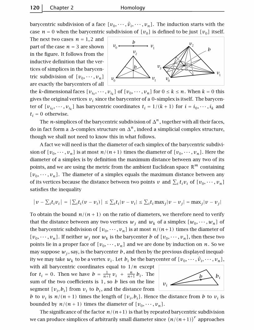
120 Chapter 2 Homology
barycentric subdivision of a face [v0, ··· , vi, ··· , vn] . The induction starts with the
case n = 0 when the barycentric subdivision of [v0] is defined to be just [v0] itself.
The next two cases n = 1,2 and
part of the case n = 3 are shown
in the figure. It follows from the
inductive definition that the ver-
tices of simplices in the barycen-
tric subdivision of [v0, ··· , vn]
are exactly the barycenters of all
the k dimensional faces [vi0 , ··· , vik] of [v0, ··· , vn] for 0 ≤ k ≤ n . When k = 0 this
gives the original vertices vi since the barycenter of a 0 simplex is itself. The barycen-
ter of [vi0 , ··· , vik] has barycentric coordinates ti = 1/(k+ 1) for i = i0, ··· , ik and
ti = 0 otherwise.
The n simplices of the barycentric subdivision of ∆n , together with all their faces,
do in fact form a ∆ complex structure on ∆n , indeed a simplicial complex structure,
though we shall not need to know this in what follows.
A fact we will need is that the diameter of each simplex of the barycentric subdivi-
sion of [v0, ··· , vn] is at most n/(n+1) times the diameter of [v0, ··· , vn] . Here the
diameter of a simplex is by definition the maximum distance between any two of its
points, and we are using the metric from the ambient Euclidean space Rm containing
[v0, ··· , vn] . The diameter of a simplex equals the maximum distance between any
of its vertices because the distance between two points v and∑i tivi of [v0, ··· , vn]
satisfies the inequality
∣∣v −∑itivi∣∣ =
∣∣∑iti(v − vi)
∣∣ ≤∑iti|v − vi| ≤∑itimaxj|v − vj| =maxj|v − vj|
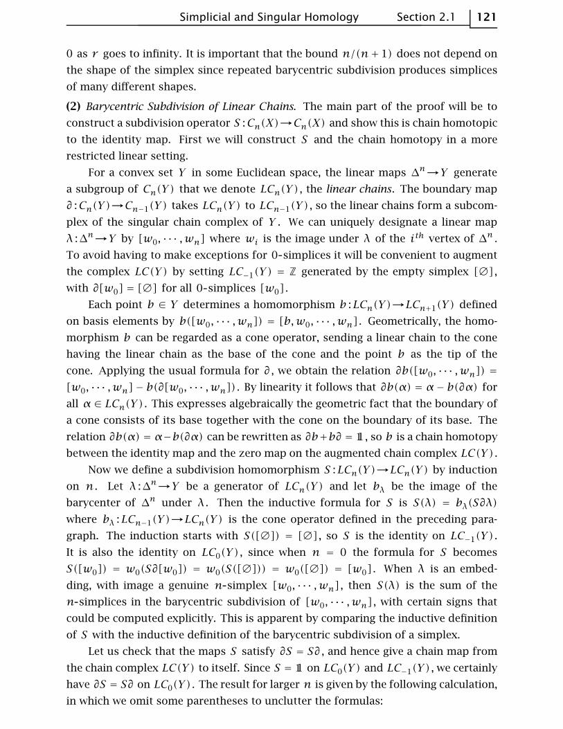
To obtain the bound n/(n+ 1) on the ratio of diameters, we therefore need to verify
that the distance between any two vertices wj and wk of a simplex [w0, ··· ,wn] of
the barycentric subdivision of [v0, ··· , vn] is at most n/(n+1) times the diameter of
[v0, ··· , vn] . If neither wj nor wk is the barycenter b of [v0, ··· , vn] , then these two
points lie in a proper face of [v0, ··· , vn] and we are done by induction on n . So we
may suppose wj , say, is the barycenter b , and then by the previous displayed inequal-
ity we may take wk to be a vertex vi . Let bi be the barycenter of [v0, ··· , vi, ··· , vn] ,
with all barycentric coordinates equal to 1/n except
for ti = 0. Then we have b = 1n+1
vi +nn+1
bi . The
sum of the two coefficients is 1, so b lies on the line
segment [vi, bi] from vi to bi , and the distance from
b to vi is n/(n+ 1) times the length of [vi, bi] . Hence the distance from b to vi is
bounded by n/(n+ 1) times the diameter of [v0, ··· , vn] .
The significance of the factor n/(n+1) is that by repeated barycentric subdivision
we can produce simplices of arbitrarily small diameter since(n/(n+1)
)rapproaches
Simplicial and Singular Homology Section 2.1 121
0 as r goes to infinity. It is important that the bound n/(n+ 1) does not depend on
the shape of the simplex since repeated barycentric subdivision produces simplices
of many different shapes.
(2) Barycentric Subdivision of Linear Chains. The main part of the proof will be to
construct a subdivision operator S :Cn(X)→Cn(X) and show this is chain homotopic
to the identity map. First we will construct S and the chain homotopy in a more
restricted linear setting.
For a convex set Y in some Euclidean space, the linear maps ∆n→Y generate
a subgroup of Cn(Y ) that we denote LCn(Y ) , the linear chains. The boundary map
∂ :Cn(Y )→Cn−1(Y ) takes LCn(Y ) to LCn−1(Y ) , so the linear chains form a subcom-
plex of the singular chain complex of Y . We can uniquely designate a linear map
λ :∆n→Y by [w0, ··· ,wn] where wi is the image under λ of the ith vertex of ∆n .
To avoid having to make exceptions for 0 simplices it will be convenient to augment
the complex LC(Y) by setting LC−1(Y ) = Z generated by the empty simplex [∅] ,
with ∂[w0] = [∅] for all 0 simplices [w0] .
Each point b ∈ Y determines a homomorphism b :LCn(Y )→LCn+1(Y ) defined
on basis elements by b([w0, ··· ,wn]) = [b,w0, ··· ,wn] . Geometrically, the homo-
morphism b can be regarded as a cone operator, sending a linear chain to the cone
having the linear chain as the base of the cone and the point b as the tip of the
cone. Applying the usual formula for ∂ , we obtain the relation ∂b([w0, ··· ,wn]) =
[w0, ··· ,wn]− b(∂[w0, ··· ,wn]) . By linearity it follows that ∂b(α) = α− b(∂α) for
all α ∈ LCn(Y ) . This expresses algebraically the geometric fact that the boundary of
a cone consists of its base together with the cone on the boundary of its base. The
relation ∂b(α) = α−b(∂α) can be rewritten as ∂b+b∂ = 11, so b is a chain homotopy
between the identity map and the zero map on the augmented chain complex LC(Y) .
Now we define a subdivision homomorphism S :LCn(Y )→LCn(Y ) by induction
on n . Let λ :∆n→Y be a generator of LCn(Y ) and let bλ be the image of the
barycenter of ∆n under λ . Then the inductive formula for S is S(λ) = bλ(S∂λ)
where bλ :LCn−1(Y )→LCn(Y ) is the cone operator defined in the preceding para-
graph. The induction starts with S([∅]) = [∅] , so S is the identity on LC−1(Y ) .
It is also the identity on LC0(Y ) , since when n = 0 the formula for S becomes
S([w0]) = w0(S∂[w0]) = w0(S([∅])) = w0([∅]) = [w0] . When λ is an embed-
ding, with image a genuine n simplex [w0, ··· ,wn] , then S(λ) is the sum of the
n simplices in the barycentric subdivision of [w0, ··· ,wn] , with certain signs that
could be computed explicitly. This is apparent by comparing the inductive definition
of S with the inductive definition of the barycentric subdivision of a simplex.
Let us check that the maps S satisfy ∂S = S∂ , and hence give a chain map from
the chain complex LC(Y) to itself. Since S = 11 on LC0(Y ) and LC−1(Y ) , we certainly
have ∂S = S∂ on LC0(Y ) . The result for larger n is given by the following calculation,
in which we omit some parentheses to unclutter the formulas:

122 Chapter 2 Homology
∂Sλ = ∂bλ(S∂λ)
= S∂λ− bλ∂(S∂λ) since ∂bλ = 11− bλ∂
= S∂λ− bλS(∂∂λ) since ∂S(∂λ) = S∂(∂λ) by induction on n
= S∂λ since ∂∂ = 0
We next build a chain homotopy T :LCn(Y )→LCn+1(Y ) between S and the iden-
tity, fitting into a diagram
We define T on LCn(Y ) inductively by setting T = 0 for n = −1 and letting Tλ =
bλ(λ − T∂λ) for n ≥ 0. The geometric motivation for this formula is an inductively
defined subdivision of ∆n×I obtained by
joining all simplices in ∆n×{0} ∪ ∂∆n×Ito the barycenter of ∆n×{1} , as indicated
in the figure in the case n = 2. What T
actually does is take the image of this sub-
division under the projection ∆n×I→∆n .
The chain homotopy formula ∂T +T∂ = 11− S is trivial on LC−1(Y ) where T = 0
and S = 11. Verifying the formula on LCn(Y ) with n ≥ 0 is done by the calculation
∂Tλ = ∂bλ(λ− T∂λ)
= λ− T∂λ− bλ∂(λ− T∂λ) since ∂bλ = 11− bλ∂
= λ− T∂λ− bλ[∂λ− ∂T(∂λ)
]
= λ− T∂λ− bλ[S(∂λ)+ T∂(∂λ)
]by induction on n
= λ− T∂λ− Sλ since ∂∂ = 0 and Sλ = bλ(S∂λ)
Now we can discard the group LC−1(Y ) and the relation ∂T + T∂ = 11 − S still
holds since T was zero on LC−1(Y ) .
(3) Barycentric Subdivision of General Chains. Define S :Cn(X)→Cn(X) by setting
Sσ = σ♯S∆n for a singular n simplex σ :∆n→X . Since S∆n is the sum of the
n simplices in the barycentric subdivision of ∆n , with certain signs, Sσ is the corre-
sponding signed sum of the restrictions of σ to the n simplices of the barycentric
subdivision of ∆n . The operator S is a chain map since
∂Sσ = ∂σ♯S∆n = σ♯∂S∆n = σ♯S∂∆n
= σ♯S(∑
i(−1)i∆ni)
where ∆ni is the ith face of ∆n
=∑i(−1)iσ♯S∆ni
=∑i(−1)iS(σ ||∆ni )
= S(∑
i(−1)iσ ||∆ni)= S(∂σ)

Simplicial and Singular Homology Section 2.1 123
In similar fashion we define T :Cn(X)→Cn+1(X) by Tσ = σ♯T∆n , and this gives a
chain homotopy between S and the identity, since the formula ∂T +T∂ = 11−S holds
by the calculation
∂Tσ = ∂σ♯T∆n = σ♯∂T∆n = σ♯(∆n − S∆n − T∂∆n) = σ − Sσ − σ♯T∂∆n
= σ − Sσ − T(∂σ)
where the last equality follows just as in the previous displayed calculation, with S
replaced by T .
(4) Iterated Barycentric Subdivision. A chain homotopy between 11 and the iterate Sm
is given by the operator Dm =∑
0≤i<m TSi since
∂Dm +Dm∂ =∑
0≤i<m
(∂TSi + TSi∂
)=
∑
0≤i<m
(∂TSi + T∂Si
)=
∑
0≤i<m
(∂T + T∂
)Si =
∑
0≤i<m
(11− S
)Si =
∑
0≤i<m
(Si − Si+1)
= 11− Sm
For each singular n simplex σ :∆n→X there exists an m such that Sm(σ) lies in
CU
n (X) since the diameter of the simplices of Sm(∆n) will be less than a Lebesgue
number of the cover of ∆n by the open sets σ−1(intUj) if m is large enough. (Recall
that a Lebesgue number for an open cover of a compact metric space is a number
ε > 0 such that every set of diameter less than ε lies in some set of the cover; such a
number exists by an elementary compactness argument.) We cannot expect the same
number m to work for all σ ’s, so let us define m(σ) to be the smallest m such that
Smσ is in CU
n (X) .
We now define D :Cn(X)→Cn+1(X) by setting Dσ = Dm(σ)σ for each singular
n simplex σ :∆n→X . For this D we would like to find a chain map ρ :Cn(X)→Cn(X)with image in CU
n (X) satisfying the chain homotopy equation
(∗) ∂D +D∂ = 11− ρ
A quick way to do this is simply to regard this equation as defining ρ , so we let
ρ = 11− ∂D −D∂ . It follows easily that ρ is a chain map since
∂ρ(σ) = ∂σ − ∂2Dσ − ∂D∂σ = ∂σ − ∂D∂σ
and ρ(∂σ) = ∂σ − ∂D∂σ −D∂2σ = ∂σ − ∂D∂σ
To check that ρ takes Cn(X) to CU
n (X) we compute ρ(σ) more explicitly:
ρ(σ) = σ − ∂Dσ −D(∂σ)
= σ − ∂Dm(σ)σ −D(∂σ)
= Sm(σ)σ +Dm(σ)(∂σ)−D(∂σ) since ∂Dm +Dm∂ = 11− Sm
The term Sm(σ)σ lies in CU
n (X) by the definition of m(σ) . The remaining terms
Dm(σ)(∂σ)−D(∂σ) are linear combinations of terms Dm(σ)(σj)−Dm(σj)(σj) for σjthe restriction of σ to a face of ∆n , so m(σj) ≤ m(σ) and hence the difference

124 Chapter 2 Homology
Dm(σ)(σj)−Dm(σj)(σj) consists of terms TSi(σj) with i ≥m(σj) , and these terms
lie in CU
n (X) since T takes CU
n−1(X) to CU
n (X) .
Viewing ρ as a chain map Cn(X)→CU
n (X) , the equation (∗) says that ∂D+D∂ =
11−ιρ for ι :CU
n (X)Cn(X) the inclusion. Furthermore, ρι = 11 since D is identically
zero on CU
n (X) , as m(σ) = 0 if σ is in CU
n(X) , hence the summation defining Dσ is
empty. Thus we have shown that ρ is a chain homotopy inverse for ι . ⊔⊓
Proof of the Excision Theorem: We prove the second version, involving a decom-
position X = A ∪ B . For the cover U = {A,B} we introduce the suggestive notation
Cn(A + B) for CU
n(X) , the sums of chains in A and chains in B . At the end of the
preceding proof we had formulas ∂D + D∂ = 11 − ιρ and ρι = 11. All the maps ap-
pearing in these formulas take chains in A to chains in A , so they induce quotient
maps when we factor out chains in A . These quotient maps automatically satisfy the
same two formulas, so the inclusion Cn(A + B)/Cn(A) Cn(X)/Cn(A) induces an
isomorphism on homology. The map Cn(B)/Cn(A∩ B)→Cn(A + B)/Cn(A) induced
by inclusion is obviously an isomorphism since both quotient groups are free with
basis the singular n simplices in B that do not lie in A . Hence we obtain the desired
isomorphism Hn(B,A∩ B) ≈ Hn(X,A) induced by inclusion. ⊔⊓
All that remains in the proof of Theorem 2.13 is to replace relative homology
groups with absolute homology groups. This is achieved by the following result.
Proposition 2.22. For good pairs (X,A) , the quotient map q : (X,A)→(X/A,A/A)induces isomorphisms q∗ :Hn(X,A)→Hn(X/A,A/A) ≈ Hn(X/A) for all n .
Proof: Let V be a neighborhood of A in X that deformation retracts onto A . We
have a commutative diagram
The upper left horizontal map is an isomorphism since in the long exact sequence of
the triple (X,V ,A) the groups Hn(V,A) are zero for all n , because a deformation
retraction of V onto A gives a homotopy equivalence of pairs (V,A) ≃ (A,A) , and
Hn(A,A) = 0. The deformation retraction of V onto A induces a deformation retrac-
tion of V/A onto A/A , so the same argument shows that the lower left horizontal
map is an isomorphism as well. The other two horizontal maps are isomorphisms
directly from excision. The right-hand vertical map q∗ is an isomorphism since q
restricts to a homeomorphism on the complement of A . From the commutativity of
the diagram it follows that the left-hand q∗ is an isomorphism. ⊔⊓
This proposition shows that relative homology can be expressed as reduced abso-
lute homology in the case of good pairs (X,A) , but in fact there is a way of doing this

Simplicial and Singular Homology Section 2.1 125
for arbitrary pairs. Consider the space X∪CA where CA is the cone (A×I)/(A×{0})
whose base A×{1} we identify with A ⊂ X . Using terminology
introduced in Chapter 0, X∪CA can also be described as the map-
ping cone of the inclusion AX . The assertion is that Hn(X,A)
is isomorphic to Hn(X ∪ CA) for all n via the sequence of iso-
morphisms
Hn(X ∪ CA) ≈ Hn(X ∪ CA,CA) ≈ Hn(X ∪ CA− {p}, CA− {p}) ≈ Hn(X,A)
where p ∈ CA is the tip of the cone. The first isomorphism comes from the exact
sequence of the pair, using the fact that CA is contractible. The second isomorphism
is excision, and the third comes from a deformation retraction of CA− {p} onto A .
Here is an application of the preceding proposition:
Example 2.23. Let us find explicit cycles representing generators of the infinite
cyclic groups Hn(Dn, ∂Dn) and Hn(S
n) . Replacing (Dn, ∂Dn) by the equivalent pair
(∆n, ∂∆n) , we will show by induction on n that the identity map in :∆n→∆n , viewed
as a singular n simplex, is a cycle generating Hn(∆n, ∂∆n) . That it is a cycle is clear
since we are considering relative homology. When n = 0 it certainly represents a
generator. For the induction step, let Λ ⊂ ∆n be the union of all but one of the
(n− 1) dimensional faces of ∆n . Then we claim there are isomorphisms
Hn(∆n, ∂∆n)≈------------→Hn−1(∂∆n,Λ)
≈←------------- Hn−1(∆n−1, ∂∆n−1)
The first isomorphism is a boundary map in the long exact sequence of the triple
(∆n, ∂∆n,Λ) , whose third terms Hi(∆n,Λ) are zero since ∆n deformation retracts
onto Λ , hence (∆n,Λ) ≃ (Λ,Λ) . The second isomorphism is induced by the inclusion
i :∆n−1→∂∆n as the face not contained in Λ . When n = 1, i induces an isomorphism
on relative homology since this is true already at the chain level. When n > 1, ∂∆n−1
is nonempty so we are dealing with good pairs and i induces a homeomorphism of
quotients ∆n−1/∂∆n−1≈ ∂∆n/Λ . The induction step then follows since the cycle in is
sent under the first isomorphism to the cycle ∂in which equals ±in−1 in Cn−1(∂∆n,Λ) .To find a cycle generating Hn(S
n) let us regard Sn as two n simplices ∆n1 and
∆n2 with their boundaries identified in the obvious way, preserving the ordering of
vertices. The difference ∆n1 −∆n2 , viewed as a singular n chain, is then a cycle, and we
claim it represents a generator of Hn(Sn) . To see this, consider the isomorphisms
Hn(Sn)
≈------------→Hn(S
n,∆n2 )≈←------------- Hn(∆n1 , ∂∆n1 )
where the first isomorphism comes from the long exact sequence of the pair (Sn,∆n2 )and the second isomorphism is justified in the nontrivial cases n > 0 by passing to
quotients as before. Under these isomorphisms the cycle ∆n1 − ∆n2 in the first group
corresponds to the cycle ∆n1 in the third group, which represents a generator of this
group as we have seen, so ∆n1 −∆n2 represents a generator of Hn(Sn) .

126 Chapter 2 Homology
The preceding proposition implies that the excision property holds also for sub-
complexes of CW complexes:
Corollary 2.24. If the CW complex X is the union of subcomplexes A and B , then
the inclusion (B,A∩B)(X,A) induces isomorphisms Hn(B,A∩B)→Hn(X,A) for
all n .
Proof: Since CW pairs are good, Proposition 2.22 allows us to pass to the quotient
spaces B/(A ∩ B) and X/A which are homeomorphic, assuming we are not in the
trivial case A∩ B = ∅ . ⊔⊓
Here is another application of the preceding proposition:
Corollary 2.25. For a wedge sum∨αXα , the inclusions iα :Xα
∨αXα induce an iso-
morphism⊕α iα∗ :
⊕α Hn(Xα)→Hn(
∨αXα) , provided that the wedge sum is formed
at basepoints xα ∈ Xα such that the pairs (Xα, xα) are good.
Proof: Since reduced homology is the same as homology relative to a basepoint, this
follows from the proposition by taking (X,A) = (∐αXα,
∐α{xα}) . ⊔⊓
Here is an application of the machinery we have developed, a classical result of
Brouwer from around 1910 known as ‘invariance of dimension’, which says in partic-
ular that Rm is not homeomorphic to Rn if m ≠ n .
Theorem 2.26. If nonempty open sets U ⊂ Rm and V ⊂ Rn are homeomorphic,
then m = n .
Proof: For x ∈ U we have Hk(U,U − {x}) ≈ Hk(Rm,Rm − {x}) by excision. From
the long exact sequence for the pair (Rm,Rm − {x}) we get Hk(Rm,Rm − {x}) ≈
Hk−1(Rm− {x}) . Since Rm − {x} deformation retracts onto a sphere Sm−1 , we con-
clude that Hk(U,U − {x}) is Z for k =m and 0 otherwise. By the same reasoning,
Hk(V,V − {y}) is Z for k = n and 0 otherwise. Since a homeomorphism h :U→Vinduces isomorphisms Hk(U,U − {x})→Hk(V,V − {h(x)}) for all k , we must have
m = n . ⊔⊓
Generalizing the idea of this proof, the local homology groups of a space X at a
point x ∈ X are defined to be the groups Hn(X,X−{x}) . For any open neighborhood
U of x , excision gives isomorphisms Hn(X,X − {x}) ≈ Hn(U,U − {x}) assuming
points are closed in X , and thus the groups Hn(X,X − {x}) depend only on the
local topology of X near x . A homeomorphism f :X→Y must induce isomorphisms
Hn(X,X − {x}) ≈ Hn(Y , Y − {f(x)}) for all x and n , so the local homology groups
can be used to tell when spaces are not locally homeomorphic at certain points, as in
the preceding proof. The exercises give some further examples of this.

Simplicial and Singular Homology Section 2.1 127
Naturality
The exact sequences we have been constructing have an extra property that will
become important later at key points in many arguments, though at first glance this
property may seem just an idle technicality, not very interesting. We shall discuss the
property now rather than interrupting later arguments to check it when it is needed,
but the reader may prefer to postpone a careful reading of this discussion.
The property is called naturality. For example, to say that the long exact sequence
of a pair is natural means that for a map f : (X,A)→(Y , B) , the diagram
is commutative. Commutativity of the squares involving i∗ and j∗ follows from the
obvious commutativity of the corresponding squares of chain groups, with Cn in place
of Hn . For the other square, when we defined induced homomorphisms we saw that
f♯∂ = ∂f♯ at the chain level. Then for a class [α] ∈ Hn(X,A) represented by a relative
cycle α , we have f∗∂[α] = f∗[∂α] = [f♯∂α] = [∂f♯α] = ∂[f♯α] = ∂f∗[α] .
Alternatively, we could appeal to the general algebraic fact that the long exact
sequence of homology groups associated to a short exact sequence of chain complexes
is natural: For a commutative diagram of short exact sequences of chain complexes
the induced diagram
is commutative. Commutativity of the first two squares is obvious since βi = i′α
implies β∗i∗ = i′∗α∗ and γj = j′β implies γ∗j∗ = j
′∗β∗ . For the third square, recall
that the map ∂ :Hn(C)→Hn−1(A) was defined by ∂[c] = [a] where c = j(b) and
i(a) = ∂b . Then ∂[γ(c)] = [α(a)] since γ(c) = γj(b) = j′(β(b)) and i′(α(a)) =
βi(a) = β∂(b) = ∂β(b) . Hence ∂γ∗[c] = α∗[a] = α∗∂[c] .

128 Chapter 2 Homology
This algebraic fact also implies naturality of the long exact sequence of a triple
and the long exact sequence of reduced homology of a pair.
Finally, there is the naturality of the long exact sequence in Theorem 2.13, that
is, commutativity of the diagram
where i and q denote inclusions and quotient maps, and f :X/A→Y/B is induced
by f . The first two squares commute since fi = if and fq = qf . The third square
expands into
We have already shown commutativity of the first and third squares, and the second
square commutes since fq = qf .
The Equivalence of Simplicial and Singular Homology
We can use the preceding results to show that the simplicial and singular homol-
ogy groups of ∆ complexes are always isomorphic. For the proof it will be convenient
to consider the relative case as well, so let X be a ∆ complex with A ⊂ X a sub-
complex. Thus A is the ∆ complex formed by any union of simplices of X . Relative
groups H∆n(X,A) can be defined in the same way as for singular homology, via relative
chains ∆n(X,A) = ∆n(X)/∆n(A) , and this yields a long exact sequence of simplicial
homology groups for the pair (X,A) by the same algebraic argument as for singular
homology. There is a canonical homomorphism H∆n(X,A)→Hn(X,A) induced by the
chain map ∆n(X,A)→Cn(X,A) sending each n simplex of X to its characteristic
map σ :∆n→X . The possibility A = ∅ is not excluded, in which case the relative
groups reduce to absolute groups.
Theorem 2.27. The homomorphisms H∆n(X,A)→Hn(X,A) are isomorphisms for
all n and all ∆ complex pairs (X,A) .
Proof: First we do the case that X is finite-dimensional and A is empty. For Xk
the k skeleton of X , consisting of all simplices of dimension k or less, we have a
commutative diagram of exact sequences:

Simplicial and Singular Homology Section 2.1 129
Let us first show that the first and fourth vertical maps are isomorphisms for all n .
The simplicial chain group ∆n(Xk, Xk−1) is zero for n ≠ k , and is free abelian with
basis the k simplices of X when n = k . Hence H∆n(Xk, Xk−1) has exactly the same
description. The corresponding singular homology groups Hn(Xk, Xk−1) can be com-
puted by considering the map Φ :∐α(∆kα, ∂∆kα)→(Xk, Xk−1) formed by the character-
istic maps ∆k→X for all the k simplices of X . Since Φ induces a homeomorphism
of quotient spaces∐α∆kα/
∐α∂∆kα ≈ Xk/Xk−1 , it induces isomorphisms on all singu-
lar homology groups. Thus Hn(Xk, Xk−1) is zero for n ≠ k , while for n = k this
group is free abelian with basis represented by the relative cycles given by the char-
acteristic maps of all the k simplices of X , in view of the fact that Hk(∆k, ∂∆k) is
generated by the identity map ∆k→∆k , as we showed in Example 2.23. Therefore the
map H∆k(Xk, Xk−1)→Hk(X
k, Xk−1) is an isomorphism.
By induction on k we may assume the second and fifth vertical maps in the pre-
ceding diagram are isomorphisms as well. The following frequently quoted basic alge-
braic lemma will then imply that the middle vertical map is an isomorphism, finishing
the proof when X is finite-dimensional and A = ∅ .
The Five-Lemma. In a commutative diagram
of abelian groups as at the right, if the two rows
are exact and α , β , δ , and ε are isomorphisms,
then γ is an isomorphism also.
Proof: It suffices to show:
(a) γ is surjective if β and δ are surjective and ε is injective.
(b) γ is injective if β and δ are injective and α is surjective.
The proofs of these two statements are straightforward diagram chasing. There is
really no choice about how the argument can proceed, and it would be a good exercise
for the reader to close the book now and reconstruct the proofs without looking.
To prove (a), start with an element c′ ∈ C′ . Then k′(c′) = δ(d) for some d ∈ D
since δ is surjective. Since ε is injective and εℓ(d) = ℓ′δ(d) = ℓ′k′(c′) = 0, we
deduce that ℓ(d) = 0, hence d = k(c) for some c ∈ C by exactness of the upper row.
The difference c′−γ(c) maps to 0 under k′ since k′(c′)−k′γ(c) = k′(c′)−δk(c) =
k′(c′)− δ(d) = 0. Therefore c′ − γ(c) = j′(b′) for some b′ ∈ B′ by exactness. Since
β is surjective, b′ = β(b) for some b ∈ B , and then γ(c + j(b)) = γ(c) + γj(b) =
γ(c)+ j′β(b) = γ(c)+ j′(b′) = c′ , showing that γ is surjective.
To prove (b), suppose that γ(c) = 0. Since δ is injective, δk(c) = k′γ(c) = 0
implies k(c) = 0, so c = j(b) for some b ∈ B . The element β(b) satisfies j′β(b) =
γj(b) = γ(c) = 0, so β(b) = i′(a′) for some a′ ∈ A′ . Since α is surjective, a′ = α(a)
for some a ∈ A . Since β is injective, β(i(a) − b) = βi(a) − β(b) = i′α(a) − β(b) =
i′(a′)−β(b) = 0 implies i(a)−b = 0. Thus b = i(a) , and hence c = j(b) = ji(a) = 0
since ji = 0. This shows γ has trivial kernel. ⊔⊓

130 Chapter 2 Homology
Returning to the proof of the theorem, we next consider the case that X is infinite-
dimensional, where we will use the following fact: A compact set in X can meet only
finitely many open simplices of X , that is, simplices with their proper faces deleted.
This is a general fact about CW complexes proved in the Appendix, but here is a
direct proof for ∆ complexes. If a compact set C intersected infinitely many open
simplices, it would contain an infinite sequence of points xi each lying in a different
open simplex. Then the sets Ui = X−⋃j≠i{xj} , which are open since their preimages
under the characteristic maps of all the simplices are clearly open, form an open cover
of C with no finite subcover.
This can be applied to show the map H∆n(X)→Hn(X) is surjective. Represent a
given element of Hn(X) by a singular n cycle z . This is a linear combination of finitely
many singular simplices with compact images, meeting only finitely many open sim-
plices of X , hence contained in Xk for some k . We have shown that H∆n(Xk)→Hn(X
k)
is an isomorphism, in particular surjective, so z is homologous in Xk (hence in X ) to
a simplicial cycle. This gives surjectivity. Injectivity is similar: If a simplicial n cycle
z is the boundary of a singular chain in X , this chain has compact image and hence
must lie in some Xk , so z represents an element of the kernel of H∆n(Xk)→Hn(X
k) .
But we know this map is injective, so z is a simplicial boundary in Xk , and therefore
in X .
It remains to do the case of arbitrary X with A ≠ ∅ , but this follows from the
absolute case by applying the five-lemma to the canonical map from the long exact
sequence of simplicial homology groups for the pair (X,A) to the corresponding long
exact sequence of singular homology groups. ⊔⊓
We can deduce from this theorem that Hn(X) is finitely generated whenever X
is a ∆ complex with finitely many n simplices, since in this case the simplicial chain
group ∆n(X) is finitely generated, hence also its subgroup of cycles and therefore
also the latter group’s quotient H∆n(X) . If we write Hn(X) as the direct sum of cyclic
groups, then the number of Z summands is known traditionally as the nth Betti
number of X , and integers specifying the orders of the finite cyclic summands are
called torsion coefficients.
It is a curious historical fact that homology was not thought of originally as a
sequence of groups, but rather as Betti numbers and torsion coefficients. One can
after all compute Betti numbers and torsion coefficients from the simplicial boundary
maps without actually mentioning homology groups. This computational viewpoint,
with homology being numbers rather than groups, prevailed from when Poincare first
started serious work on homology around 1900, up until the 1920s when the more
abstract viewpoint of groups entered the picture. During this period ‘homology’ meant
primarily ‘simplicial homology’, and it was another 20 years before the shift to singular
homology was complete, with the final definition of singular homology emerging only

Simplicial and Singular Homology Section 2.1 131
in a 1944 paper of Eilenberg, after contributions from quite a few others, particularly
Alexander and Lefschetz. Within the next few years the rest of the basic structure
of homology theory as we have presented it fell into place, and the first definitive
treatment appeared in the classic book [Eilenberg & Steenrod 1952].
Exercises
1. What familiar space is the quotient ∆ complex of a 2 simplex [v0, v1, v2] obtained
by identifying the edges [v0, v1] and [v1, v2] , preserving the ordering of vertices?
2. Show that the ∆ complex obtained from ∆3 by performing the edge identifications
[v0, v1] ∼ [v1, v3] and [v0, v2] ∼ [v2, v3] deformation retracts onto a Klein bottle.
Find other pairs of identifications of edges that produce ∆ complexes deformation
retracting onto a torus, a 2 sphere, and RP2 .
3. Construct a ∆ complex structure on RPn as a quotient of a ∆ complex structure
on Sn having vertices the two vectors of length 1 along each coordinate axis in Rn+1 .
4. Compute the simplicial homology groups of the triangular parachute obtained from
∆2 by identifying its three vertices to a single point.
5. Compute the simplicial homology groups of the Klein bottle using the ∆ complex
structure described at the beginning of this section.
6. Compute the simplicial homology groups of the ∆ complex obtained from n + 1
2 simplices ∆20, ··· ,∆2
n by identifying all three edges of ∆20 to a single edge, and for
i > 0 identifying the edges [v0, v1] and [v1, v2] of ∆2i to a single edge and the edge
[v0, v2] to the edge [v0, v1] of ∆2i−1 .
7. Find a way of identifying pairs of faces of ∆3 to produce a ∆ complex structure
on S3 having a single 3 simplex, and compute the simplicial homology groups of this
∆ complex.
8. Construct a 3 dimensional ∆ complex X from n tetrahe-
dra T1, ··· , Tn by the following two steps. First arrange the
tetrahedra in a cyclic pattern as in the figure, so that each Tishares a common vertical face with its two neighbors Ti−1
and Ti+1 , subscripts being taken mod n . Then identify the
bottom face of Ti with the top face of Ti+1 for each i . Show the simplicial homology
groups of X in dimensions 0, 1, 2, 3 are Z , Zn , 0 , Z , respectively. [The space X is
an example of a lens space; see Example 2.43 for the general case.]
9. Compute the homology groups of the ∆ complex X obtained from ∆n by identi-
fying all faces of the same dimension. Thus X has a single k simplex for each k ≤ n .
10. (a) Show the quotient space of a finite collection of disjoint 2 simplices obtained
by identifying pairs of edges is always a surface, locally homeomorphic to R2 .
(b) Show the edges can always be oriented so as to define a ∆ complex structure on
the quotient surface. [This is more difficult.]

132 Chapter 2 Homology
11. Show that if A is a retract of X then the map Hn(A)→Hn(X) induced by the
inclusion A ⊂ X is injective.
12. Show that chain homotopy of chain maps is an equivalence relation.
13. Verify that f ≃ g implies f∗ = g∗ for induced homomorphisms of reduced
homology groups.
14. Determine whether there exists a short exact sequence 0→Z4→Z8⊕Z2→Z4→0.
More generally, determine which abelian groups A fit into a short exact sequence
0→Zpm→A→Zpn→0 with p prime. What about the case of short exact sequences
0→Z→A→Zn→0?
15. For an exact sequence A→B→C→D→E show that C = 0 iff the map A→Bis surjective and D→E is injective. Hence for a pair of spaces (X,A) , the inclusion
AX induces isomorphisms on all homology groups iff Hn(X,A) = 0 for all n .
16. (a) Show that H0(X,A) = 0 iff A meets each path-component of X .
(b) Show that H1(X,A) = 0 iff H1(A)→H1(X) is surjective and each path-component
of X contains at most one path-component of A .
17. (a) Compute the homology groups Hn(X,A) when X is S2 or S1×S1 and A is a
finite set of points in X .
(b) Compute the groups Hn(X,A) and Hn(X, B) for X
a closed orientable surface of genus two with A and B
the circles shown. [What are X/A and X/B ?]
18. Show that for the subspace Q ⊂ R , the relative homology group H1(R,Q) is free
abelian and find a basis.
19. Compute the homology groups of the subspace of I×I consisting of the four
boundary edges plus all points in the interior whose first coordinate is rational.
20. Show that Hn(X) ≈ Hn+1(SX) for all n , where SX is the suspension of X . More
generally, thinking of SX as the union of two cones CX with their bases identified,
compute the reduced homology groups of the union of any finite number of cones
CX with their bases identified.
21. Making the preceding problem more concrete, construct explicit chain maps
s :Cn(X)→Cn+1(SX) inducing isomorphisms Hn(X)→Hn+1(SX) .
22. Prove by induction on dimension the following facts about the homology of a
finite-dimensional CW complex X , using the observation that Xn/Xn−1 is a wedge
sum of n spheres:
(a) If X has dimension n then Hi(X) = 0 for i > n and Hn(X) is free.
(b) Hn(X) is free with basis in bijective correspondence with the n cells if there are
no cells of dimension n− 1 or n+ 1.
(c) If X has k n cells, then Hn(X) is generated by at most k elements.

Simplicial and Singular Homology Section 2.1 133
23. Show that the second barycentric subdivision of a ∆ complex is a simplicial
complex. Namely, show that the first barycentric subdivision produces a ∆ complex
with the property that each simplex has all its vertices distinct, then show that for a
∆ complex with this property, barycentric subdivision produces a simplicial complex.
24. Show that each n simplex in the barycentric subdivision of ∆n is defined by n
inequalities ti0 ≤ ti1 ≤ ··· ≤ tin in its barycentric coordinates, where (i0, ··· , in) is a
permutation of (0, ··· , n) .
25. Find an explicit, noninductive formula for the barycentric subdivision operator
S :Cn(X)→Cn(X) .
26. Show that H1(X,A) is not isomorphic to H1(X/A) if X = [0,1] and A is the
sequence 1, 1/2,1/3, ··· together with its limit 0. [See Example 1.25.]
27. Let f : (X,A)→(Y , B) be a map such that both f :X→Y and the restriction
f :A→B are homotopy equivalences.
(a) Show that f∗ :Hn(X,A)→Hn(Y , B) is an isomorphism for all n .
(b) For the case of the inclusion f : (Dn, Sn−1) (Dn,Dn − {0}) , show that f is not
a homotopy equivalence of pairs — there is no g : (Dn,Dn − {0})→(Dn, Sn−1) such
that fg and gf are homotopic to the identity through maps of pairs. [Observe that
a homotopy equivalence of pairs (X,A)→(Y , B) is also a homotopy equivalence for
the pairs obtained by replacing A and B by their closures.]
28. Let X be the cone on the 1 skeleton of ∆3 , the union of all line segments joining
points in the six edges of ∆3 to the barycenter of ∆3 . Compute the local homology
groups Hn(X,X − {x}) for all x ∈ X . Define ∂X to be the subspace of points x
such that Hn(X,X − {x}) = 0 for all n , and compute the local homology groups
Hn(∂X, ∂X−{x}) . Use these calculations to determine which subsets A ⊂ X have the
property that f(A) ⊂ A for all homeomorphisms f :X→X .
29. Show that S1×S1 and S1
∨ S1∨ S2 have isomorphic homology groups in all
dimensions, but their universal covering spaces do not.
30. In each of the following commutative diagrams assume that all maps but one are
isomorphisms. Show that the remaining map must be an isomorphism as well.
31. Using the notation of the five-lemma, give an example where the maps α , β , δ ,
and ε are zero but γ is nonzero. This can be done with short exact sequences in
which all the groups are either Z or 0.

134 Chapter 2 Homology
Now that the basic properties of homology have been established, we can begin
to move a little more freely. Our first topic, exploiting the calculation of Hn(Sn) , is
Brouwer’s notion of degree for maps Sn→Sn . Historically, Brouwer’s introduction of
this concept in the years 1910–12 preceded the rigorous development of homology,
so his definition was rather different, using the technique of simplicial approximation
which we explain in §2.C. The later definition in terms of homology is certainly more
elegant, though perhaps with some loss of geometric intuition. More in the spirit of
Brouwer’s definition is a third approach using differential topology, presented very
lucidly in [Milnor 1965].
Degree
For a map f :Sn→Sn with n > 0, the induced map f∗ :Hn(Sn)→Hn(S
n) is a
homomorphism from an infinite cyclic group to itself and so must be of the form
f∗(α) = dα for some integer d depending only on f . This integer is called the
degree of f , with the notation deg f . Here are some basic properties of degree:
(a) deg 11 = 1, since 11∗ = 11.
(b) deg f = 0 if f is not surjective. For if we choose a point x0 ∈ Sn−f(Sn) then f
can be factored as a composition Sn→Sn − {x0} Sn and Hn(Sn− {x0}) = 0
since Sn − {x0} is contractible. Hence f∗ = 0.
(c) If f ≃ g then deg f = degg since f∗ = g∗ . The converse statement, that f ≃ g
if deg f = degg , is a fundamental theorem of Hopf from around 1925 which we
prove in Corollary 4.25.
(d) deg fg = deg f degg , since (fg)∗ = f∗g∗ . As a consequence, deg f = ±1 if f
is a homotopy equivalence since fg ≃ 11 implies deg f degg = deg 11 = 1.
(e) deg f = −1 if f is a reflection of Sn , fixing the points in a subsphere Sn−1
and interchanging the two complementary hemispheres. For we can give Sn a
∆ complex structure with these two hemispheres as its two n simplices ∆n1 and
∆n2 , and the n chain ∆n1 − ∆n2 represents a generator of Hn(Sn) as we saw in
Example 2.23, so the reflection interchanging ∆n1 and ∆n2 sends this generator to
its negative.
(f) The antipodal map −11 :Sn→Sn , x֏ −x , has degree (−1)n+1 since it is the
composition of n + 1 reflections, each changing the sign of one coordinate in
Rn+1 .
(g) If f :Sn→Sn has no fixed points then deg f = (−1)n+1 . For if f(x) ≠ x then the
line segment from f(x) to −x , defined by t֏ (1− t)f (x)− tx for 0 ≤ t ≤ 1,
does not pass through the origin. Hence if f has no fixed points, the formula
ft(x) = [(1 − t)f (x) − tx]/|(1 − t)f (x) − tx| defines a homotopy from f to

Computations and Applications Section 2.2 135
the antipodal map. Note that the antipodal map has no fixed points, so the fact
that maps without fixed points are homotopic to the antipodal map is a sort of
converse statement.
Here is an interesting application of degree:
Theorem 2.28. Sn has a continuous field of nonzero tangent vectors iff n is odd.
Proof: Suppose x֏ v(x) is a tangent vector field on Sn , assigning to a vector
x ∈ Sn the vector v(x) tangent to Sn at x . Regarding v(x) as a vector at the origin
instead of at x , tangency just means that x and v(x) are orthogonal in Rn+1 . If
v(x) ≠ 0 for all x , we may normalize so that |v(x)| = 1 for all x by replacing v(x)
by v(x)/|v(x)| . Assuming this has been done, the vectors (cos t)x + (sin t)v(x) lie
in the unit circle in the plane spanned by x and v(x) . Letting t go from 0 to π , we
obtain a homotopy ft(x) = (cos t)x+ (sin t)v(x) from the identity map of Sn to the
antipodal map −11. This implies that deg(−11) = deg 11, hence (−1)n+1= 1 and n
must be odd.
Conversely, if n is odd, say n = 2k−1, we can define v(x1, x2, ··· , x2k−1, x2k) =
(−x2, x1, ··· ,−x2k, x2k−1) . Then v(x) is orthogonal to x , so v is a tangent vector
field on Sn , and |v(x)| = 1 for all x ∈ Sn . ⊔⊓
For the much more difficult problem of finding the maximum number of tan-
gent vector fields on Sn that are linearly independent at each point, see [VBKT] or
[Husemoller 1966].
Another nice application of degree, giving a partial answer to a question raised in
Example 1.43, is the following result:
Proposition 2.29. Z2 is the only nontrivial group that can act freely on Sn if n is
even.
Recall that an action of a group G on a space X is a homomorphism from G
to the group Homeo(X) of homeomorphisms X→X , and the action is free if the
homeomorphism corresponding to each nontrivial element of G has no fixed points.
In the case of Sn , the antipodal map x֏−x generates a free action of Z2 .
Proof: Since the degree of a homeomorphism must be ±1, an action of a group G
on Sn determines a degree function d :G→{±1} . This is a homomorphism since
deg fg = deg f degg . If the action is free, then d sends every nontrivial element of
G to (−1)n+1 by property (g) above. Thus when n is even, d has trivial kernel, so
G ⊂ Z2 . ⊔⊓
Next we describe a technique for computing degrees which can be applied to most
maps that arise in practice. Suppose f :Sn→Sn , n > 0, has the property that for

136 Chapter 2 Homology
some point y ∈ Sn , the preimage f−1(y) consists of only finitely many points, say
x1, ··· , xm . Let U1, ··· , Um be disjoint neighborhoods of these points, mapped by f
into a neighborhood V of y . Then f(Ui − xi) ⊂ V − y for each i , and we have a
diagram
where all the maps are the obvious ones, and in particular ki and pi are induced
by inclusions, so the triangles and squares commute. The two isomorphisms in the
upper half of the diagram come from excision, while the lower two isomorphisms come
from exact sequences of pairs. Via these four isomorphisms, the top two groups in the
diagram can be identified with Hn(Sn) ≈ Z , and the top homomorphism f∗ becomes
multiplication by an integer called the local degree of f at xi , written deg f ||xi .
For example, if f is a homeomorphism, then y can be any point and there is
only one corresponding xi , so all the maps in the diagram are isomorphisms and
deg f ||xi = deg f = ±1. More generally, if f maps each Ui homeomorphically onto
V , then deg f ||xi = ±1 for each i . This situation occurs quite often in applications,
and it is usually not hard to determine the correct signs.
Here is the formula that reduces degree calculations to computing local degrees:
Proposition 2.30. deg f =∑i deg f ||xi .
Proof: By excision, the central term Hn(Sn, Sn − f−1(y)
)in the preceding diagram
is the direct sum of the groups Hn(Ui, Ui − xi) ≈ Z , with ki the inclusion of the
ith summand and pi the projection onto the ith summand. Identifying the outer
groups in the diagram with Z as before, commutativity of the lower triangle says that
pij(1) = 1, hence j(1) = (1, ··· ,1) =∑i ki(1) . Commutativity of the upper square
says that the middle f∗ takes ki(1) to deg f ||xi , hence the sum∑i ki(1) = j(1)
is taken to∑i deg f ||xi . Commutativity of the lower square then gives the formula
deg f =∑i deg f ||xi . ⊔⊓
Example 2.31. We can use this result to construct a map Sn→Sn of any given degree,
for each n ≥ 1. Let q :Sn→∨kSn be the quotient map obtained by collapsing the
complement of k disjoint open balls Bi in Sn to a point, and let p :∨kSn→Sn identify
all the summands to a single sphere. Consider the composition f = pq . For almost all
y ∈ Sn we have f−1(y) consisting of one point xi in each Bi . The local degree of f
at xi is ±1 since f is a homeomorphism near xi . By precomposing p with reflections
of the summands of∨kSn if necessary, we can make each local degree either +1 or
−1, whichever we wish. Thus we can produce a map Sn→Sn of degree ±k .

Computations and Applications Section 2.2 137
Example 2.32. In the case of S1 , the map f(z) = zk , where we view S1 as the unit
circle in C , has degree k . This is evident in the case k = 0 since f is then constant.
The case k < 0 reduces to the case k > 0 by composing with z֏ z−1 , which is a
reflection, of degree −1. To compute the degree when k > 0, observe first that for
any y ∈ S1 , f−1(y) consists of k points x1, ··· , xk near each of which f is a local
homeomorphism, stretching a circular arc by a factor of k . This local stretching can
be eliminated by a deformation of f near xi that does not change local degree, so the
local degree at xi is the same as for a rotation of S1 . A rotation is a homeomorphism
so its local degree at any point equals its global degree, which is +1 since a rotation
is homotopic to the identity. Hence deg f ||xi = 1 and deg f = k .
Another way of obtaining a map Sn→Sn of degree k is to take a repeated sus-
pension of the map z֏ zk in Example 2.32, since suspension preserves degree:
Proposition 2.33. deg Sf = deg f , where Sf :Sn+1→Sn+1 is the suspension of the
map f :Sn→Sn .
Proof: Let CSn denote the cone (Sn×I)/(Sn×1) with base Sn = Sn×0 ⊂ CSn ,
so CSn/Sn is the suspension of Sn . The map f induces Cf : (CSn, Sn)→(CSn, Sn)with quotient Sf . The naturality of the boundary maps
in the long exact sequence of the pair (CSn, Sn) then
gives commutativity of the diagram at the right. Hence
if f∗ is multiplication by d , so is Sf∗ . ⊔⊓
Note that for f :Sn→Sn , the suspension Sf maps only one point to each of the
two ‘poles’ of Sn+1 . This implies that the local degree of Sf at each pole must equal
the global degree of Sf . Thus the local degree of a map Sn→Sn can be any integer
if n ≥ 2, just as the degree itself can be any integer when n ≥ 1.
Cellular Homology
Cellular homology is a very efficient tool for computing the homology groups of
CW complexes, based on degree calculations. Before giving the definition of cellular
homology, we first establish a few preliminary facts:
Lemma 2.34. If X is a CW complex, then :
(a) Hk(Xn, Xn−1) is zero for k ≠ n and is free abelian for k = n , with a basis in
one-to-one correspondence with the n cells of X .
(b) Hk(Xn) = 0 for k > n . In particular, if X is finite-dimensional then Hk(X) = 0
for k > dimX .
(c) The map Hk(Xn)→Hk(X) induced by the inclusion XnX is an isomorphism
for k < n and surjective for k = n .
Proof: Statement (a) follows immediately from the observation that (Xn, Xn−1) is a
good pair and Xn/Xn−1 is a wedge sum of n spheres, one for each n cell of X . Here

138 Chapter 2 Homology
we are using Proposition 2.22 and Corollary 2.25. Next consider the following part of
the long exact sequence of the pair (Xn, Xn−1) :
Hk+1(Xn, Xn−1) -→Hk(X
n−1) -→Hk(Xn) -→Hk(X
n, Xn−1)
If k ≠ n the last term is zero by part (a) so the middle map is surjective, while if
k ≠ n− 1 then the first term is zero so the middle map is injective. Now look at the
inclusion-induced homomorphisms
Hk(X0) -→Hk(X
1) -→··· -→Hk(Xk−1) -→Hk(X
k) -→Hk(Xk+1) -→···
By what we have just shown these are all isomorphisms except that the map to Hk(Xk)
may not be surjective and the map from Hk(Xk) may not be injective. The first part
of the sequence then gives statement (b) since Hk(X0) = 0 when k > 0. Also, the last
part of the sequence gives (c) when X is finite-dimensional.
The proof of (c) when X is infinite-dimensional requires more work, and this can
be done in two different ways. The more direct approach is to descend to the chain
level and use the fact that a singular chain in X has compact image, hence meets only
finitely many cells of X by Proposition A.1 in the Appendix. Thus each chain lies
in a finite skeleton Xm . So a k cycle in X is a cycle in some Xm , and then by the
finite-dimensional case of (c), the cycle is homologous to a cycle in Xn if n ≥ k , so
Hk(Xn)→Hk(X) is surjective. Similarly for injectivity, if a k cycle in Xn bounds a
chain in X , this chain lies in some Xm with m ≥ n , so by the finite-dimensional case
the cycle bounds a chain in Xn if n > k .
The other approach is more general. From the long exact sequence of the pair
(X,Xn) it suffices to show Hk(X,Xn) = 0 for k ≤ n . Since Hk(X,X
n) ≈ Hk(X/Xn) ,
this reduces the problem to showing:
(∗) Hk(X) = 0 for k ≤ n if the n skeleton of X is a point.
When X is finite-dimensional, (∗) is immediate from the finite-dimensional case
of (c) which we have already shown. It will suffice therefore to reduce the infinite-
dimensional case to the finite-dimensional case. This reduction will be achieved by
stretching X out to a complex that is at least locally finite-dimensional, using a special
case of the ‘mapping telescope’ construction described in greater generality in §3.F.
Consider X×[0,∞) with its product cell structure,
where we give [0,∞) the cell structure with the integer
points as 0 cells. Let T =⋃iX
i×[i,∞) , a subcomplex
of X×[0,∞) . The figure shows a schematic picture of T with [0,∞) in the hor-
izontal direction and the subcomplexes Xi×[i, i + 1] as rectangles whose size in-
creases with i since Xi ⊂ Xi+1 . The line labeled R can be ignored for now. We claim
that T ≃ X , hence Hk(X) ≈ Hk(T) for all k . Since X is a deformation retract of
X×[0,∞) , it suffices to show that X×[0,∞) also deformation retracts onto T . Let
Yi = T∪(X×[i,∞)
). Then Yi deformation retracts onto Yi+1 since X×[i, i+1] defor-
mation retracts onto Xi×[i, i+1]∪X×{i+1} by Proposition 0.16. If we perform the

Computations and Applications Section 2.2 139
deformation retraction of Yi onto Yi+1 during the t interval [1− 1/2i,1− 1/2i+1] ,
then this gives a deformation retraction ft of X×[0,∞) onto T , with points in
Xi×[0,∞) stationary under ft for t ≥ 1 − 1/2i+1 . Continuity follows from the fact
that CW complexes have the weak topology with respect to their skeleta, so a map is
continuous if its restriction to each skeleton is continuous.
Recalling that X0 is a point, let R ⊂ T be the ray X0×[0,∞) and let Z ⊂ T be the
union of this ray with all the subcomplexes Xi×{i} . Then Z/R is homeomorphic to∨iX
i , a wedge sum of finite-dimensional complexes with n skeleton a point, so the
finite-dimensional case of (∗) together with Corollary 2.25 describing the homology
of wedge sums implies that Hk(Z/R) = 0 for k ≤ n . The same is therefore true for Z ,
from the long exact sequence of the pair (Z,R) , since R is contractible. Similarly, T/Z
is a wedge sum of finite-dimensional complexes with (n+ 1) skeleton a point, since
if we first collapse each subcomplex Xi×{i} of T to a point, we obtain the infinite
sequence of suspensions SXi ‘skewered’ along the ray R , and then if we collapse R to
a point we obtain∨iΣXi where ΣXi is the reduced suspension of Xi , obtained from
SXi by collapsing the line segment X0×[i, i+1] to a point, so ΣXi has (n+1) skeleton
a point. Thus Hk(T/Z) = 0 for k ≤ n+ 1. The long exact sequence of the pair (T ,Z)
then implies that Hk(T) = 0 for k ≤ n , and we have proved (∗) . ⊔⊓
Let X be a CW complex. Using Lemma 2.34, portions of the long exact sequences
for the pairs (Xn+1, Xn) , (Xn, Xn−1) , and (Xn−1, Xn−2) fit into a diagram
where dn+1 and dn are defined as the compositions jn∂n+1 and jn−1∂n , which are
just ‘relativizations’ of the boundary maps ∂n+1 and ∂n . The composition dndn+1
includes two successive maps in one of the exact sequences, hence is zero. Thus the
horizontal row in the diagram is a chain complex, called the cellular chain complex
of X since Hn(Xn, Xn−1) is free with basis in one-to-one correspondence with the
n cells of X , so one can think of elements of Hn(Xn, Xn−1) as linear combinations
of n cells of X . The homology groups of this cellular chain complex are called the
cellular homology groups of X . Temporarily we denote them HCWn (X) .
Theorem 2.35. HCWn (X) ≈ Hn(X) .

140 Chapter 2 Homology
Proof: From the diagram above, Hn(X) can be identified with Hn(Xn)/ Im ∂n+1 .
Since jn is injective, it maps Im ∂n+1 isomorphically onto Im(jn∂n+1) = Imdn+1
and Hn(Xn) isomorphically onto Im jn = Ker ∂n . Since jn−1 is injective, Ker ∂n =
Kerdn . Thus jn induces an isomorphism of the quotient Hn(Xn)/ Im ∂n+1 onto
Kerdn/ Imdn+1 . ⊔⊓
Here are a few immediate applications:
(i) Hn(X) = 0 if X is a CW complex with no n cells.
(ii) More generally, if X is a CW complex with k n cells, then Hn(X) is generated
by at most k elements. For since Hn(Xn, Xn−1) is free abelian on k generators,
the subgroup Kerdn must be generated by at most k elements, hence also the
quotient Kerdn/ Imdn+1 .
(iii) If X is a CW complex having no two of its cells in adjacent dimensions, then
Hn(X) is free abelian with basis in one-to-one correspondence with the n cells
of X . This is because the cellular boundary maps dn are automatically zero in
this case.
This last observation applies for example to CPn , which has a CW structure with one
cell of each even dimension 2k ≤ 2n as we saw in Example 0.6. Thus
Hi(CPn) ≈
{Z for i = 0,2,4, ··· ,2n0 otherwise
Another simple example is Sn×Sn with n > 1, using the product CW structure con-
sisting of a 0 cell, two n cells, and a 2n cell.
It is possible to prove the statements (i)–(iii) for finite-dimensional CW complexes
by induction on the dimension, without using cellular homology but only the basic
results from the previous section. However, the viewpoint of cellular homology makes
(i)–(iii) quite transparent.
Next we describe how the cellular boundary maps dn can be computed. When
n = 1 this is easy since the boundary map d1 :H1(X1, X0)→H0(X
0) is the same as
the simplicial boundary map ∆1(X)→∆0(X) . In case X is connected and has only
one 0 cell, then d1 must be 0, otherwise H0(X) would not be Z . When n > 1 we will
show that dn can be computed in terms of degrees:
Cellular Boundary Formula. dn(enα) =
∑β dαβe
n−1β where dαβ is the degree of the
map Sn−1α →X
n−1→Sn−1β that is the composition of the attaching map of enα with
the quotient map collapsing Xn−1− en−1
β to a point.
Here we are identifying the cells enα and en−1β with generators of the corresponding
summands of the cellular chain groups. The summation in the formula contains only
finitely many terms since the attaching map of enα has compact image, so this image
meets only finitely many cells en−1β .
To derive the cellular boundary formula, consider the commutative diagram

Computations and Applications Section 2.2 141
where:
Φα is the characteristic map of the cell enα and ϕα is its attaching map.
q :Xn−1→Xn−1/Xn−2 is the quotient map.
qβ :Xn−1/Xn−2→Sn−1β collapses the complement of the cell en−1
β to a point, the
resulting quotient sphere being identified with Sn−1β = Dn−1
β /∂Dn−1β via the char-
acteristic map Φβ .
∆αβ : ∂Dnα→Sn−1β is the composition qβqϕα , in other words, the attaching map
of enα followed by the quotient map Xn−1→Sn−1β collapsing the complement of
en−1β in Xn−1 to a point.
The map Φα∗ takes a chosen generator [Dnα] ∈ Hn(Dnα , ∂D
nα) to a generator of the Z
summand of Hn(Xn, Xn−1) corresponding to enα . Letting enα denote this generator,
commutativity of the left half of the diagram then gives dn(enα) = jn−1ϕα∗∂[D
nα] . In
terms of the basis for Hn−1(Xn−1, Xn−2) corresponding to the cells en−1
β , the map qβ∗is the projection of Hn−1(X
n−1/Xn−2) onto its Z summand corresponding to en−1β .
Commutativity of the diagram then yields the formula for dn given above.
Example 2.36. Let Mg be the closed orientable surface of genus g with its usual CW
structure consisting of one 0 cell, 2g 1 cells, and one 2 cell attached by the product
of commutators [a1, b1] ··· [ag, bg] . The associated cellular chain complex is
0 -----→Zd2------------→Z
2g d1------------→Z -----→0
As observed above, d1 must be 0 since there is only one 0 cell. Also, d2 is 0 because
each ai or bi appears with its inverse in [a1, b1] ··· [ag, bg] , so the maps ∆αβ are
homotopic to constant maps. Since d1 and d2 are both zero, the homology groups
of Mg are the same as the cellular chain groups, namely, Z in dimensions 0 and 2,
and Z2g in dimension 1.
Example 2.37. The closed nonorientable surface Ng of genus g has a cell structure
with one 0 cell, g 1 cells, and one 2 cell attached by the word a21a
22 ···a
2g . Again
d1 = 0, and d2 :Z→Zg is specified by the equation d2(1) = (2, ··· ,2) since each ai
appears in the attaching word of the 2 cell with total exponent 2, which means that
each ∆αβ is homotopic to the map z֏z2 , of degree 2. Since d2(1) = (2, ··· ,2) , we
have d2 injective and hence H2(Ng) = 0. If we change the basis for Zg by replacing
the last standard basis element (0, ··· ,0,1) by (1, ··· ,1) , we see that H1(Ng) ≈
Zg−1⊕Z2 .

142 Chapter 2 Homology
These two examples illustrate the general fact that the orientability of a closed
connected manifold M of dimension n is detected by Hn(M) , which is Z if M is
orientable and 0 otherwise. This is shown in Theorem 3.26.
Example 2.38: An Acyclic Space. Let X be obtained from S1∨ S1 by attaching two
2 cells by the words a5b−3 and b3(ab)−2 . Then d2 :Z2→Z2 has matrix
(5 −2−3 1
),
with the two columns coming from abelianizing a5b−3 and b3(ab)−2 to 5a − 3b
and −2a + b , in additive notation. The matrix has determinant −1, so d2 is an
isomorphism and Hi(X) = 0 for all i . Such a space X is called acyclic.
We can see that this acyclic space is not contractible by considering π1(X) , which
has the presentation⟨a,b |||| a
5b−3, b3(ab)−2 ⟩ . There is a nontrivial homomorphism
from this group to the group G of rotational symmetries of a regular dodecahedron,
sending a to the rotation ρa through angle 2π/5 about the axis through the center
of a pentagonal face, and b to the rotation ρb through angle 2π/3 about the axis
through a vertex of this face. The composition ρaρb is a rotation through angle π
about the axis through the midpoint of an edge abutting this vertex. Thus the relations
a5= b3
= (ab)2 defining π1(X) become ρ5a = ρ
3b = (ρaρb)
2= 1 in G , which means
there is a well-defined homomorphism ρ :π1(X)→G sending a to ρa and b to ρb .
It is not hard to see that G is generated by ρa and ρb , so ρ is surjective. With
more work one can compute that the kernel of ρ is Z2 , generated by the element
a5= b3
= (ab)2 , and this Z2 is in fact the center of π1(X) . In particular, π1(X) has
order 120 since G has order 60.
After these 2 dimensional examples, let us now move up to three dimensions,
where we have the additional task of computing the cellular boundary map d3 .
Example 2.39. A 3 dimensional torus
T 3= S1
×S1×S1 can be constructed
from a cube by identifying each pair
of opposite square faces as in the first
of the two figures. The second figure
shows a slightly different pattern of
identifications of opposite faces, with the front and back faces now identified via a
rotation of the cube around a horizontal left-right axis. The space produced by these
identifications is the product K×S1 of a Klein bottle and a circle. For both T 3 and
K×S1 we have a CW structure with one 3 cell, three 2 cells, three 1 cells, and one
0 cell. The cellular chain complexes thus have the form
0 -→Zd3------------→Z
3 d2------------→Z3 0-----→Z -→0
In the case of the 3 torus T 3 the cellular boundary map d2 is zero by the same
calculation as for the 2 dimensional torus. We claim that d3 is zero as well. This
amounts to saying that the three maps ∆αβ :S2→S2 corresponding to the three 2 cells

Computations and Applications Section 2.2 143
have degree zero. Each ∆αβ maps the interiors of two opposite faces of the cube
homeomorphically onto the complement of a point in the target S2 and sends the
remaining four faces to this point. Computing local degrees at the center points of
the two opposite faces, we see that the local degree is +1 at one of these points and
−1 at the other, since the restrictions of ∆αβ to these two faces differ by a reflection
of the boundary of the cube across the plane midway between them, and a reflection
has degree −1. Since the cellular boundary maps are all zero, we deduce that Hi(T3)
is Z for i = 0,3, Z3 for i = 1,2, and 0 for i > 3.
For K×S1 , when we compute local degrees for the front and back faces we find
that the degrees now have the same rather than opposite signs since the map ∆αβ on
these two faces differs not by a reflection but by a rotation of the boundary of the cube.
The local degrees for the other faces are the same as before. Using the letters A , B , C
to denote the 2 cells given by the faces orthogonal to the edges a , b , c , respectively,
we have the boundary formulas d3e3= 2C , d2A = 2b , d2B = 0, and d2C = 0. It
follows that H3(K×S1) = 0, H2(K×S
1) = Z⊕Z2 , and H1(K×S1) = Z⊕Z⊕Z2 .
Many more examples of a similar nature, quotients of a cube or other polyhedron
with faces identified in some pattern, could be worked out in similar fashion. But let
us instead turn to some higher-dimensional examples.
Example 2.40: Moore Spaces. Given an abelian group G and an integer n ≥ 1, we
will construct a CW complex X such that Hn(X) ≈ G and Hi(X) = 0 for i ≠ n . Such a
space is called a Moore space, commonly written M(G,n) to indicate the dependence
on G and n . It is probably best for the definition of a Moore space to include the
condition that M(G,n) be simply-connected if n > 1. The spaces we construct will
have this property.
As an easy special case, when G = Zm we can take X to be Sn with a cell en+1
attached by a map Sn→Sn of degree m . More generally, any finitely generated G can
be realized by taking wedge sums of examples of this type for finite cyclic summands
of G , together with copies of Sn for infinite cyclic summands of G .
In the general nonfinitely generated case let F→G be a homomorphism of a free
abelian group F onto G , sending a basis for F onto some set of generators of G . The
kernel K of this homomorphism is a subgroup of a free abelian group, hence is itself
free abelian. Choose bases {xα} for F and {yβ} for K , and write yβ =∑α dβαxα .
Let Xn =∨αS
nα , so Hn(X
n) ≈ F via Corollary 2.25. We will construct X from Xn by
attaching cells en+1β via maps fβ :Sn→Xn such that the composition of fβ with the
projection onto the summand Snα has degree dβα . Then the cellular boundary map
dn+1 will be the inclusion K F , hence X will have the desired homology groups.
The construction of fβ generalizes the construction in Example 2.31 of a map
Sn→Sn of given degree. Namely, we can let fβ map the complement of∑α |dβα|

144 Chapter 2 Homology
disjoint balls in Sn to the 0 cell of Xn while sending |dβα| of the balls onto the
summand Snα by maps of degree +1 if dβα > 0, or degree −1 if dβα < 0.
Example 2.41. By taking a wedge sum of the Moore spaces constructed in the preced-
ing example for varying n we obtain a connected CW complex with any prescribed
sequence of homology groups in dimensions 1,2,3, ··· .
Example 2.42: Real Projective Space RPn . As we saw in Example 0.4, RPn has a CW
structure with one cell ek in each dimension k ≤ n , and the attaching map for ek is the
2 sheeted covering projection ϕ :Sk−1→RPk−1 . To compute the boundary map dkwe compute the degree of the composition Sk−1 ϕ
-----→RPk−1 q-----→RPk−1/RPk−2
= Sk−1 ,
with q the quotient map. The map qϕ restricts to a homeomorphism from each
component of Sk−1− Sk−2 onto RPk−1
−RPk−2 , and these two homeomorphisms are
obtained from each other by precomposing with the antipodal map of Sk−1 , which
has degree (−1)k . Hence degqϕ = deg 11+deg(−11) = 1+ (−1)k , and so dk is either
0 or multiplication by 2 according to whether k is odd or even. Thus the cellular
chain complex for RPn is
0 -→Z2-----→Z
0-----→···
2-----→Z
0-----→Z
2-----→Z
0-----→Z -→0 if n is even
0 -→Z0-----→Z
2-----→···
2-----→Z
0-----→Z
2-----→Z
0-----→Z -→0 if n is odd
From this it follows that
Hk(RPn) =
Z for k = 0 and for k = n odd
Z2 for k odd, 0 < k < n0 otherwise
Example 2.43: Lens Spaces. This example is somewhat more complicated. Given an
integer m > 1 and integers ℓ1, ··· , ℓn relatively prime to m , define the lens space L =
Lm(ℓ1, ··· , ℓn) to be the orbit space S2n−1/Zm of the unit sphere S2n−1⊂ C
n with the
action of Zm generated by the rotation ρ(z1, ··· , zn) = (e2πiℓ1/mz1, ··· , e
2πiℓn/mzn) ,
rotating the j th C factor of Cn by the angle 2πℓj/m . In particular, when m = 2, ρ
is the antipodal map, so L = RP2n−1 in this case. In the general case, the projection
S2n−1→L is a covering space since the action of Zm on S2n−1 is free: Only the identity
element fixes any point of S2n−1 since each point of S2n−1 has some coordinate zjnonzero and then e2πikℓj/mzj ≠ zj for 0 < k < m , as a result of the assumption that
ℓj is relatively prime to m .
We shall construct a CW structure on L with one cell ek for each k ≤ 2n− 1 and
show that the resulting cellular chain complex is
0 -→Z0-----→Z
m------------→Z
0-----→···
0-----→Z
m------------→Z
0-----→Z -→0
with boundary maps alternately 0 and multiplication by m . Hence
Hk(Lm(ℓ1, ··· , ℓn)
)=
Z for k = 0,2n− 1
Zm for k odd, 0 < k < 2n− 1
0 otherwise

Computations and Applications Section 2.2 145
To obtain the CW structure, first subdivide the unit circle C in the nth C factor
of Cn by taking the points e2πij/m∈ C as vertices, j = 1, ··· ,m . Joining the j th
vertex of C to the unit sphere S2n−3⊂ C
n−1 by arcs of great circles in S2n−1 yields
a (2n− 2) dimensional ball B2n−2j bounded by S2n−3 . Specifically, B2n−2
j consists of
the points cosθ (0, ··· ,0, e2πij/m)+sinθ (z1, ··· , zn−1,0) for 0 ≤ θ ≤ π/2. Similarly,
joining the j th edge of C to S2n−3 gives a ball B2n−1j bounded by B2n−2
j and B2n−2j+1 ,
subscripts being taken mod m . The rotation ρ carries S2n−3 to itself and rotates C
by the angle 2πℓn/m , hence ρ permutes the B2n−2j ’s and the B2n−1
j ’s. A suitable
power of ρ , namely ρr where rℓn ≡ 1 mod m , takes each B2n−2j and B2n−1
j to the
next one. Since ρr has order m , it is also a generator of the rotation group Zm , and
hence we may obtain L as the quotient of one B2n−1j by identifying its two faces B2n−2
j
and B2n−2j+1 together via ρr .
In particular, when n = 2, B2n−1j is a lens-shaped
3 ball and L is obtained from this ball by identifying its
two curved disk faces via ρr , which may be described as
the composition of the reflection across the plane con-
taining the rim of the lens, taking one face of the lens to
the other, followed by a rotation of this face through the
angle 2πℓ/m where ℓ = rℓ1 . The figure illustrates the
case (m,ℓ) = (7,2) , with the two dots indicating a typical pair of identified points in
the upper and lower faces of the lens. Since the lens space L is determined by the rota-
tion angle 2πℓ/m , it is conveniently written Lℓ/m . Clearly only the mod m value of ℓ
matters. It is a classical theorem of Reidemeister from the 1930s that Lℓ/m is homeo-
morphic to Lℓ′/m′ iff m′=m and ℓ′ ≡ ±ℓ±1 mod m . For example, when m = 7 there
are only two distinct lens spaces L1/7 and L2/7 . The ‘if’ part of this theorem is easy:
Reflecting the lens through a mirror shows that Lℓ/m ≈ L−ℓ/m , and by interchanging
the roles of the two C factors of C2 one obtains Lℓ/m ≈ Lℓ−1/m . In the converse di-
rection, Lℓ/m ≈ Lℓ′/m′ clearly implies m =m′ since π1(Lℓ/m) ≈ Zm . The rest of the
theorem takes considerably more work, involving either special 3 dimensional tech-
niques or more algebraic methods that generalize to classify the higher-dimensional
lens spaces as well. The latter approach is explained in [Cohen 1973].
Returning to the construction of a CW structure on Lm(ℓ1, ··· , ℓn) , observe that
the (2n − 3) dimensional lens space Lm(ℓ1, ··· , ℓn−1) sits in Lm(ℓ1, ··· , ℓn) as the
quotient of S2n−3 , and Lm(ℓ1, ··· , ℓn) is obtained from this subspace by attaching
two cells, of dimensions 2n− 2 and 2n− 1, coming from the interiors of B2n−1j and
its two identified faces B2n−2j and B2n−2
j+1 . Inductively this gives a CW structure on
Lm(ℓ1, ··· , ℓn) with one cell ek in each dimension k ≤ 2n− 1.
The boundary maps in the associated cellular chain complex are computed as
follows. The first one, d2n−1 , is zero since the identification of the two faces of
B2n−1j is via a reflection (degree −1) across B2n−1
j fixing S2n−3 , followed by a rota-

146 Chapter 2 Homology
tion (degree +1), so d2n−1(e2n−1) = e2n−2
− e2n−2= 0. The next boundary map
d2n−2 takes e2n−2 to me2n−3 since the attaching map for e2n−2 is the quotient map
S2n−3→Lm(ℓ1, ··· , ℓn−1) and the balls B2n−3j in S2n−3 which project down onto e2n−3
are permuted cyclically by the rotation ρ of degree +1. Inductively, the subsequent
boundary maps dk then alternate between 0 and multiplication by m .
Also of interest are the infinite-dimensional lens spaces Lm(ℓ1, ℓ2, ···) = S∞/Zm
defined in the same way as in the finite-dimensional case, starting from a sequence of
integers ℓ1, ℓ2, ··· relatively prime to m . The space Lm(ℓ1, ℓ2, ···) is the union of the
increasing sequence of finite-dimensional lens spaces Lm(ℓ1, ··· , ℓn) for n = 1,2, ··· ,
each of which is a subcomplex of the next in the cell structure we have just con-
structed, so Lm(ℓ1, ℓ2, ···) is also a CW complex. Its cellular chain complex consists
of a Z in each dimension with boundary maps alternately 0 and m , so its reduced
homology consists of a Zm in each odd dimension.
In the terminology of §1.B, the infinite-dimensional lens space Lm(ℓ1, ℓ2, ···) is
an Eilenberg–MacLane space K(Zm,1) since its universal cover S∞ is contractible, as
we showed there. By Theorem 1B.8 the homotopy type of Lm(ℓ1, ℓ2, ···) depends
only on m , and not on the ℓi ’s. This is not true in the finite-dimensional case, when
two lens spaces Lm(ℓ1, ··· , ℓn) and Lm(ℓ′1, ··· , ℓ
′n) have the same homotopy type
iff ℓ1 ··· ℓn ≡ ±knℓ′1 ···ℓ
′n mod m for some integer k . A proof of this is outlined in
Exercise 2 in §3.E and Exercise 29 in §4.2. For example, the 3 dimensional lens spaces
L1/5 and L2/5 are not homotopy equivalent, though they have the same fundamental
group and the same homology groups. On the other hand, L1/7 and L2/7 are homotopy
equivalent but not homeomorphic.
Euler Characteristic
For a finite CW complex X , the Euler characteristic χ(X) is defined to be the
alternating sum∑n(−1)ncn where cn is the number of n cells of X , generalizing
the familiar formula vertices − edges + faces for 2 dimensional complexes. The
following result shows that χ(X) can be defined purely in terms of homology, and
hence depends only on the homotopy type of X . In particular, χ(X) is independent
of the choice of CW structure on X .
Theorem 2.44. χ(X) =∑n(−1)n rankHn(X) .
Here the rank of a finitely generated abelian group is the number of Z summands
when the group is expressed as a direct sum of cyclic groups. We shall need the
following fact, whose proof we leave as an exercise: If 0→A→B→C→0 is a short
exact sequence of finitely generated abelian groups, then rank B = rankA+ rankC .
Proof of 2.44: This is purely algebraic. Let
0 -→Ckdk------------→Ck−1 -→··· -→C1
d1------------→C0 -→0

Computations and Applications Section 2.2 147
be a chain complex of finitely generated abelian groups, with cycles Zn = Kerdn ,
boundaries Bn = Imdn+1 , and homology Hn = Zn/Bn . Thus we have short exact
sequences 0→Zn→Cn→Bn−1→0 and 0→Bn→Zn→Hn→0, hence
rankCn = rankZn + rank Bn−1
rankZn = rank Bn + rankHn
Now substitute the second equation into the first, multiply the resulting equation by
(−1)n , and sum over n to get∑n(−1)n rankCn =
∑n(−1)n rankHn . Applying this
with Cn = Hn(Xn, Xn−1) then gives the theorem. ⊔⊓
For example, the surfaces Mg and Ng have Euler characteristics χ(Mg) = 2−2g
and χ(Ng) = 2−g . Thus all the orientable surfaces Mg are distinguished from each
other by their Euler characteristics, as are the nonorientable surfaces Ng , and there
are only the relations χ(Mg) = χ(N2g) .
Split Exact Sequences
Suppose one has a retraction r :X→A , so ri = 11 where i :A→X is the inclusion.
The induced map i∗ :Hn(A)→Hn(X) is then injective since r∗i∗ = 11. From this it
follows that the boundary maps in the long exact sequence for (X,A) are zero, so the
long exact sequence breaks up into short exact sequences
0 -→Hn(A)i∗-----→Hn(X)
j∗-----→Hn(X,A) -→0
The relation r∗i∗ = 11 actually gives more information than this, by the following
piece of elementary algebra:
Splitting Lemma. For a short exact sequence 0 -→Ai-----→ B
j-----→ C -→ 0 of abelian
groups the following statements are equivalent :
(a) There is a homomorphism p :B→A such that pi = 11 :A→A .
(b) There is a homomorphism s :C→B such that js = 11 :C→C .
(c) There is an isomorphism B ≈ A⊕C making
a commutative diagram as at the right, where
the maps in the lower row are the obvious ones,
a֏ (a,0) and (a, c)֏ c .
If these conditions are satisfied, the exact sequence is said to split. Note that (c)
is symmetric: There is no essential difference between the roles of A and C .
Sketch of Proof: For the implication (a) ⇒ (c) one checks that the map B→A⊕C ,
b֏(p(b), j(b)
), is an isomorphism with the desired properties. For (b) ⇒ (c) one
uses instead the map A⊕C→B , (a, c)֏ i(a) + s(c) . The opposite implications
(c) ⇒ (a) and (c) ⇒ (b) are fairly obvious. If one wants to show (b) ⇒ (a) directly,
one can define p(b) = i−1(b − sj(b)) . Further details are left to the reader. ⊔⊓

148 Chapter 2 Homology
Except for the implications (b)⇒ (a) and (b)⇒ (c) , the proof works equally well
for nonabelian groups. In the nonabelian case, (b) is definitely weaker than (a) and (c),
and short exact sequences satisfying (b) only determine B as a semidirect product of
A and C . The difficulty is that s(C) might not be a normal subgroup of B . In the
nonabelian case one defines ‘splitting’ to mean that (b) is satisfied.
In both the abelian and nonabelian contexts, if C is free then every exact sequence
0→Ai-----→B
j-----→C→0 splits, since one can define s :C→B by choosing a basis {cα}
for C and letting s(cα) be any element bα ∈ B such that j(bα) = cα . The converse
is also true: If every short exact sequence ending in C splits, then C is free. This is
because for every C there is a short exact sequence 0→A→B→C→0 with B free
— choose generators for C and let B have a basis in one-to-one correspondence with
these generators, then let B→C send each basis element to the corresponding gen-
erator — so if this sequence 0→A→B→C→0 splits, C is isomorphic to a subgroup
of a free group, hence is free.
From the Splitting Lemma and the remarks preceding it we deduce that a retrac-
tion r :X→A gives a splitting Hn(X) ≈ Hn(A)⊕Hn(X,A) . This can be used to show
the nonexistence of such a retraction in some cases, for example in the situation of
the Brouwer fixed point theorem, where a retraction Dn→Sn−1 would give an im-
possible splitting Hn−1(Dn) ≈ Hn−1(S
n−1)⊕Hn−1(Dn, Sn−1) . For a somewhat more
subtle example, consider the mapping cylinder Mf of a degree m map f :Sn→Sn
with m > 1. If Mf retracted onto the Sn ⊂ Mf corresponding to the domain of f ,
we would have a split short exact sequence
But this sequence does not split since Z is not isomorphic to Z⊕Zm if m > 1, so the
retraction cannot exist. In the simplest case of the degree 2 map S1→S1 , z֏ z2 ,
this says that the Mobius band does not retract onto its boundary circle.
Homology of Groups
In §1.B we constructed for each group G a CW complex K(G,1) having a con-
tractible universal cover, and we showed that the homotopy type of such a space
K(G,1) is uniquely determined by G . The homology groups Hn(K(G,1)
)therefore
depend only on G , and are usually denoted simply Hn(G) . The calculations for lens
spaces in Example 2.43 show that Hn(Zm) is Zm for odd n and 0 for even n > 0.
Since S1 is a K(Z,1) and the torus is a K(Z×Z,1) , we also know the homology of
these two groups. More generally, the homology of finitely generated abelian groups
can be computed from these examples using the Kunneth formula in §3.B and the fact
that a product K(G,1)×K(H,1) is a K(G×H,1) .
Here is an application of the calculation of Hn(Zm) :

Computations and Applications Section 2.2 149
Proposition 2.45. If a finite-dimensional CW complex X is a K(G,1) , then the group
G = π1(X) must be torsionfree.
This applies to quite a few manifolds, for example closed surfaces other than
S2 and RP2 , and also many 3 dimensional manifolds such as complements of knots
in S3 .
Proof: If G had torsion, it would have a finite cyclic subgroup Zm for some m > 1,
and the covering space of X corresponding to this subgroup of G = π1(X) would
be a K(Zm,1) . Since X is a finite-dimensional CW complex, the same would be true
of its covering space K(Zm,1) , and hence the homology of the K(Zm,1) would be
nonzero in only finitely many dimensions. But this contradicts the fact that Hn(Zm)
is nonzero for infinitely many values of n . ⊔⊓
Reflecting the richness of group theory, the homology of groups has been studied
quite extensively. A good starting place for those wishing to learn more is the text-
book [Brown 1982]. At a more advanced level the books [Adem & Milgram 1994] and
[Benson 1992] treat the subject from a mostly topological viewpoint.
Mayer–Vietoris Sequences
In addition to the long exact sequence of homology groups for a pair (X,A) , there
is another sort of long exact sequence, known as a Mayer–Vietoris sequence, which
is equally powerful but is sometimes more convenient to use. For a pair of subspaces
A , B ⊂ X such that X is the union of the interiors of A and B , this exact sequence
has the form
··· -→Hn(A∩ B)Φ------------→Hn(A)⊕Hn(B)
Ψ------------→Hn(X)
∂------------→Hn−1(A∩ B) -→···
··· -→H0(X) -→0
In addition to its usefulness for calculations, the Mayer–Vietoris sequence is also ap-
plied frequently in induction arguments, where one might know that a certain state-
ment is true for A , B , and A∩B by induction and then deduce that it is true for A∪B
by the exact sequence.
The Mayer–Vietoris sequence is easy to derive from the machinery of §2.1. Let
Cn(A+ B) be the subgroup of Cn(X) consisting of chains that are sums of chains in
A and chains in B . The usual boundary map ∂ :Cn(X)→Cn−1(X) takes Cn(A+B) to
Cn−1(A+B) , so the Cn(A+B) ’s form a chain complex. According to Proposition 2.21,
the inclusions Cn(A + B) Cn(X) induce isomorphisms on homology groups. The
Mayer–Vietoris sequence is then the long exact sequence of homology groups asso-
ciated to the short exact sequence of chain complexes formed by the short exact
sequences
0 -→Cn(A∩ B)ϕ------------→Cn(A)⊕ Cn(B)
ψ------------→Cn(A+ B) -→0

150 Chapter 2 Homology
where ϕ(x) = (x,−x) and ψ(x,y) = x + y . The exactness of this short exact
sequence can be checked as follows. First, Kerϕ = 0 since a chain in A ∩ B that
is zero as a chain in A (or in B ) must be the zero chain. Next, Imϕ ⊂ Kerψ since
ψϕ = 0. Also, Kerψ ⊂ Imϕ since for a pair (x,y) ∈ Cn(A)⊕Cn(B) the condition
x + y = 0 implies x = −y , so x is a chain in both A and B , that is, x ∈ Cn(A∩ B) ,
and (x,y) = (x,−x) ∈ Imϕ . Finally, exactness at Cn(A+ B) is immediate from the
definition of Cn(A+ B) .
The boundary map ∂ :Hn(X)→Hn−1(A∩ B) can easily be made explicit. A class
α ∈ Hn(X) is represented by a cycle z , and by barycentric subdivision or some other
method we can choose z to be a sum x+y of chains in A and B , respectively. It need
not be true that x and y are cycles individually, but ∂x = −∂y since ∂(x + y) = 0,
and the element ∂α ∈ Hn−1(A∩ B) is represented by the cycle ∂x = −∂y , as is clear
from the definition of the boundary map in the long exact sequence of homology
groups associated to a short exact sequence of chain complexes.
There is also a formally identical Mayer–Vietoris sequence for reduced homology
groups, obtained by augmenting the previous short exact sequence of chain complexes
in the obvious way:
Mayer–Vietoris sequences can be viewed as analogs of the van Kampen theorem
since if A∩B is path-connected, the H1 terms of the reduced Mayer–Vietoris sequence
yield an isomorphism H1(X) ≈(H1(A)⊕H1(B)
)/ ImΦ . This is exactly the abelianized
statement of the van Kampen theorem, and H1 is the abelianization of π1 for path-
connected spaces, as we show in §2.A.
There are also Mayer–Vietoris sequences for decompositions X = A∪B such that
A and B are deformation retracts of neighborhoods U and V with U∩V deformation
retracting onto A∩B . Under these assumptions the five-lemma implies that the maps
Cn(A + B)→Cn(U + V) induce isomorphisms on homology, and hence so do the
maps Cn(A + B)→Cn(X) , which was all that we needed to obtain a Mayer–Vietoris
sequence. For example, if X is a CW complex and A and B are subcomplexes, then
we can choose for U and V neighborhoods of the form Nε(A) and Nε(B) constructed
in the Appendix, which have the property that Nε(A)∩Nε(B) = Nε(A∩ B) .
Example 2.46. Take X = Sn with A and B the northern and southern hemispheres,
so that A ∩ B = Sn−1 . Then in the reduced Mayer–Vietoris sequence the terms
Hi(A)⊕Hi(B) are zero, so we obtain isomorphisms Hi(Sn) ≈ Hi−1(S
n−1) . This gives
another way of calculating the homology groups of Sn by induction.
Example 2.47. We can decompose the Klein bottle K as the union of two Mobius
bands A and B glued together by a homeomorphism between their boundary circles.

Computations and Applications Section 2.2 151
Then A , B , and A ∩ B are homotopy equivalent to circles, so the interesting part of
the reduced Mayer–Vietoris sequence for the decomposition K = A∪B is the segment
0 -→H2(K) -→H1(A∩ B)Φ-----→H1(A)⊕H1(B) -→H1(K) -→0
The map Φ is Z→Z⊕Z , 1֏(2,−2) , since the boundary circle of a Mobius band wraps
twice around the core circle. Since Φ is injective we obtain H2(K) = 0. Furthermore,
we have H1(K) ≈ Z⊕Z2 since we can choose (1,0) and (1,−1) as a basis for Z⊕Z . All
the higher homology groups of K are zero from the earlier part of the Mayer–Vietoris
sequence.
Example 2.48. Let us describe an exact sequence which is somewhat similar to the
Mayer–Vietoris sequence and which in some cases generalizes it. If we are given two
maps f ,g :X→Y then we can form a quotient space Z of the disjoint union of X×I
and Y via the identifications (x,0) ∼ f(x) and (x,1) ∼ g(x) , thus attaching one
end of X×I to Y by f and the other end by g . For example, if f and g are each the
identity map X→X then Z = X×S1 . If only one of f and g , say f , is the identity
map, then Z is homeomorphic to what is called the mapping torus of g , the quotient
space of X×I under the identifications (x,0) ∼ (g(x),1) . The Klein bottle is an
example, with g a reflection S1→S1 .
The exact sequence we want has the form
(∗) ··· ----→Hn(X)f∗−g∗----------------------------→Hn(Y )
i∗---------→Hn(Z) ----→Hn−1(X)f∗−g∗----------------------------→Hn−1(Y ) ----→···
where i is the evident inclusion Y Z . To derive this exact sequence, consider
the map q : (X×I,X×∂I)→(Z, Y ) that is the restriction to X×I of the quotient map
X×I ∐ Y→Z . The map q induces a map of long exact sequences:
In the upper row the middle term is the direct sum of two copies of Hn(X) , and the
map i∗ is surjective since X×I deformation retracts onto X×{0} and X×{1} . Sur-
jectivity of the maps i∗ in the upper row implies that the next maps are 0, which
in turn implies that the maps ∂ are injective. Thus the map ∂ in the upper row
gives an isomorphism of Hn+1(X×I,X×∂I) onto the kernel of i∗ , which consists of
the pairs (α,−α) for α ∈ Hn(X) . This kernel is a copy of Hn(X) , and the middle
vertical map q∗ takes (α,−α) to f∗(α) − g∗(α) . The left-hand q∗ is an isomor-
phism since these are good pairs and q induces a homeomorphism of quotient spaces
(X×I)/(X×∂I)→Z/Y . Hence if we replace Hn+1(Z, Y ) in the lower exact sequence
by the isomorphic group Hn(X) ≈ Ker i∗ we obtain the long exact sequence we want.
In the case of the mapping torus of a reflection g :S1→S1 , with Z a Klein bottle,
the interesting portion of the exact sequence (∗) is

152 Chapter 2 Homology
Thus H2(Z) = 0 and we have a short exact sequence 0→Z2→H1(Z)→Z→0. This
splits since Z is free, so H1(Z) ≈ Z2⊕Z . Other examples are given in the Exercises.
If Y is the disjoint union of spaces Y1 and Y2 , with f :X→Y1 and g :X→Y2 ,
then Z consists of the mapping cylinders of these two maps with their domain ends
identified. For example, suppose we have a CW complex decomposed as the union of
two subcomplexes A and B and we take f and g to be the inclusions A∩BA and
A ∩ B B . Then the double mapping cylinder Z is homotopy equivalent to A ∪ B
since we can view Z as (A∩ B)×I with A and B attached at the two ends, and then
slide the attaching of A down to the B end to produce A∪B with (A∩B)× I attached
at one of its ends. By Proposition 0.18 the sliding operation preserves homotopy type,
so we obtain a homotopy equivalence Z ≃ A∪B . The exact sequence (∗) in this case
is the Mayer–Vietoris sequence.
A relative form of the Mayer–Vietoris sequence is sometimes useful. If one has
a pair of spaces (X, Y ) = (A ∪ B,C ∪ D) with C ⊂ A and D ⊂ B , such that X is the
union of the interiors of A and B , and Y is the union of the interiors of C and D ,
then there is a relative Mayer–Vietoris sequence
··· -→Hn(A∩ B,C ∩D)Φ------------→Hn(A,C)⊕Hn(B,D)
Ψ------------→Hn(X, Y )
∂------------→ ···
To derive this, consider the commutative diagram
where Cn(A + B,C + D) is the quotient of the subgroup Cn(A + B) ⊂ Cn(X) by its
subgroup Cn(C + D) ⊂ Cn(Y ) . Thus the three columns of the diagram are exact.
We have seen that the first two rows are exact, and we claim that the third row is
exact also, with the maps ϕ and ψ induced from the ϕ and ψ in the second row.
Since ψϕ = 0 in the second row, this holds also in the third row, so the third row
is at least a chain complex. Viewing the three rows as chain complexes, the diagram
then represents a short exact sequence of chain complexes. The associated long exact
sequence of homology groups has two out of every three terms zero since the first
two rows of the diagram are exact. Hence the remaining homology groups are zero
and the third row is exact.

Computations and Applications Section 2.2 153
The third column maps to 0→Cn(Y )→Cn(X)→Cn(X, Y )→0, inducing maps of
homology groups that are isomorphisms for the X and Y terms as we have seen above.
So by the five-lemma the maps Cn(A+B,C+D)→Cn(X, Y ) also induce isomorphisms
on homology. The relative Mayer–Vietoris sequence is then the long exact sequence
of homology groups associated to the short exact sequence of chain complexes given
by the third row of the diagram.
Homology with Coefficients
There is an easy generalization of the homology theory we have considered so
far that behaves in a very similar fashion and sometimes offers technical advantages.
The generalization consists of using chains of the form∑iniσi where each σi is
a singular n simplex in X as before, but now the coefficients ni are taken to lie
in a fixed abelian group G rather than Z . Such n chains form an abelian group
Cn(X;G) , and there is the expected relative version Cn(X,A;G) = Cn(X;G)/Cn(A;G) .
The old formula for the boundary maps ∂ can still be used for arbitrary G , namely
∂(∑
iniσi)=∑i,j(−1)jniσi ||[v0, ··· , vj, ··· , vn] . Just as before, a calculation shows
that ∂2= 0, so the groups Cn(X;G) and Cn(X,A;G) form chain complexes. The
resulting homology groups Hn(X;G) and Hn(X,A;G) are called homology groups
with coefficients in G. Reduced groups Hn(X;G) are defined via the augmented chain
complex ··· -→C0(X;G)ε-----→G -→0 with ε again defined by summing coefficients.
The case G = Z2 is particularly simple since one is just considering sums of sin-
gular simplices with coefficients 0 or 1, so by discarding terms with coefficient 0
one can think of chains as just finite ‘unions’ of singular simplices. The boundary
formulas also simplify since one no longer has to worry about signs. Since signs are
an algebraic representation of orientation considerations, one can also ignore orien-
tations. This means that homology with Z2 coefficients is often the most natural tool
in the absence of orientability.
All the theory we developed in §2.1 for Z coefficients carries over directly to
general coefficient groups G with no change in the proofs. The same is true for Mayer–
Vietoris sequences. Differences between Hn(X;G) and Hn(X) begin to appear only
when one starts making calculations. When X is a point, the method used to compute
Hn(X) shows that Hn(X;G) is G for n = 0 and 0 for n > 0. From this it follows
just as for G = Z that Hn(Sk;G) is G for n = k and 0 otherwise.
Cellular homology also generalizes to homology with coefficients, with the cellu-
lar chain group Hn(Xn, Xn−1) replaced by Hn(X
n, Xn−1;G) , which is a direct sum of
G ’s, one for each n cell. The proof that the cellular homology groups HCWn (X) agree
with singular homology Hn(X) extends immediately to give HCWn (X;G) ≈ Hn(X;G) .
The cellular boundary maps are given by the same formula as for Z coefficients,
dn(∑
αnαenα
)=∑α,β dαβnαe
n−1β . The old proof applies, but the following result is
needed to know that the coefficients dαβ are the same as before:

154 Chapter 2 Homology
Lemma 2.49. If f :Sk→Sk has degree m , then f∗ :Hk(Sk;G)→Hk(S
k;G) is multi-
plication by m .
Proof: As a preliminary observation, note that a homomorphism ϕ :G1→G2 induces
maps ϕ♯ :Cn(X,A;G1)→Cn(X,A;G2) commuting with boundary maps, so there are
induced homomorphisms ϕ∗ :Hn(X,A;G1)→Hn(X,A;G2) . These have various nat-
urality properties. For example, they give a commutative diagram mapping the long
exact sequence of homology for the pair (X,A) with G1 coefficients to the correspond-
ing sequence with G2 coefficients. Also, the maps ϕ∗ commute with homomorphisms
f∗ induced by maps f : (X,A)→(Y , B) .Now let f :Sk→Sk have degree m and let ϕ :Z→G take 1 to a given element
g ∈ G . Then we have a commutative
diagram as at the right, where commu-
tativity of the outer two squares comes
from the inductive calculation of these
homology groups, reducing to the case k = 0 when the commutativity is obvious.
Since the diagram commutes, the assumption that the map across the top takes
1 to m implies that the map across the bottom takes g to mg . ⊔⊓
Example 2.50. It is instructive to see what happens to the homology of RPn when
the coefficient group G is chosen to be a field F . The cellular chain complex is
···0-----→F
2-----→F
0-----→F
2-----→F
0-----→F -→0
Hence if F has characteristic 2, for example if F = Z2 , then Hk(RPn;F) ≈ F for
0 ≤ k ≤ n , a more uniform answer than with Z coefficients. On the other hand, if
F has characteristic different from 2 then the boundary maps F2-----→ F are isomor-
phisms, hence Hk(RPn;F) is F for k = 0 and for k = n odd, and is zero otherwise.
In §3.A we will see that there is a general algebraic formula expressing homology
with arbitrary coefficients in terms of homology with Z coefficients. Some easy special
cases that give much of the flavor of the general result are included in the Exercises.
In spite of the fact that homology with Z coefficients determines homology with
other coefficient groups, there are many situations where homology with a suitably
chosen coefficient group can provide more information than homology with Z coef-
ficients. A good example of this is the proof of the Borsuk–Ulam theorem using Z2
coefficients in §2.B.
As another illustration, we will now give an example of a map f :X→Y with the
property that the induced maps f∗ are trivial for homology with Z coefficients but
not for homology with Zm coefficients for suitably chosen m . Thus homology with
Zm coefficients tells us that f is not homotopic to a constant map, which we would
not know using only Z coefficients.

Computations and Applications Section 2.2 155
Example 2.51. Let X be a Moore space M(Zm, n) obtained from Sn by attaching a
cell en+1 by a map of degree m . The quotient map f :X→X/Sn = Sn+1 induces
trivial homomorphisms on reduced homology with Z coefficients since the nonzero
reduced homology groups of X and Sn+1 occur in different dimensions. But with Zm
coefficients the story is different, as we can see by considering the long exact sequence
of the pair (X, Sn) , which contains the segment
0 = Hn+1(Sn;Zm) -→Hn+1(X;Zm)
f∗-----→Hn+1(X/S
n;Zm)
Exactness says that f∗ is injective, hence nonzero since Hn+1(X;Zm) is Zm , the cel-
lular boundary map Hn+1(Xn+1, Xn;Zm)→Hn(X
n, Xn−1;Zm) being Zmm-----→Zm .
Exercises
1. Prove the Brouwer fixed point theorem for maps f :Dn→Dn by applying degree
theory to the map Sn→Sn that sends both the northern and southern hemispheres
of Sn to the southern hemisphere via f . [This was Brouwer’s original proof.]
2. Given a map f :S2n→S2n , show that there is some point x ∈ S2n with either
f(x) = x or f(x) = −x . Deduce that every map RP2n→RP2n has a fixed point.
Construct maps RP2n−1→RP2n−1 without fixed points from linear transformations
R2n→R
2n without eigenvectors.
3. Let f :Sn→Sn be a map of degree zero. Show that there exist points x,y ∈ Sn
with f(x) = x and f(y) = −y . Use this to show that if F is a continuous vector
field defined on the unit ball Dn in Rn such that F(x) ≠ 0 for all x , then there exists
a point on ∂Dn where F points radially outward and another point on ∂Dn where F
points radially inward.
4. Construct a surjective map Sn→Sn of degree zero, for each n ≥ 1.
5. Show that any two reflections of Sn across different n dimensional hyperplanes
are homotopic, in fact homotopic through reflections. [The linear algebra formula for
a reflection in terms of inner products may be helpful.]
6. Show that every map Sn→Sn can be homotoped to have a fixed point if n > 0.
7. For an invertible linear transformation f :Rn→Rn show that the induced map
on Hn(Rn,Rn − {0}) ≈ Hn−1(R
n− {0}) ≈ Z is 11 or −11 according to whether the
determinant of f is positive or negative. [Use Gaussian elimination to show that the
matrix of f can be joined by a path of invertible matrices to a diagonal matrix with
±1’s on the diagonal.]
8. A polynomial f(z) with complex coefficients, viewed as a map C→C , can always
be extended to a continuous map of one-point compactifications f :S2→S2 . Show
that the degree of f equals the degree of f as a polynomial. Show also that the local
degree of f at a root of f is the multiplicity of the root.

156 Chapter 2 Homology
9. Compute the homology groups of the following 2 complexes:
(a) The quotient of S2 obtained by identifying north and south poles to a point.
(b) S1×(S1
∨ S1) .
(c) The space obtained from D2 by first deleting the interiors of two disjoint subdisks
in the interior of D2 and then identifying all three resulting boundary circles
together via homeomorphisms preserving clockwise orientations of these circles.
(d) The quotient space of S1×S1 obtained by identifying points in the circle S1
×{x0}
that differ by 2π/m rotation and identifying points in the circle {x0}×S1 that
differ by 2π/n rotation.
10. Let X be the quotient space of S2 under the identifications x ∼ −x for x in the
equator S1 . Compute the homology groups Hi(X) . Do the same for S3 with antipodal
points of the equatorial S2⊂ S3 identified.
11. In an exercise for §1.2 we described a 3 dimensional CW complex obtained from
the cube I3 by identifying opposite faces via a one-quarter twist. Compute the ho-
mology groups of this complex.
12. Show that the quotient map S1×S1→S2 collapsing the subspace S1
∨ S1 to a
point is not nullhomotopic by showing that it induces an isomorphism on H2 . On the
other hand, show via covering spaces that any map S2→S1×S1 is nullhomotopic.
13. Let X be the 2 complex obtained from S1 with its usual cell structure by attaching
two 2 cells by maps of degrees 2 and 3, respectively.
(a) Compute the homology groups of all the subcomplexes A ⊂ X and the corre-
sponding quotient complexes X/A .
(b) Show that X ≃ S2 and that the only subcomplex A ⊂ X for which the quotient
map X→X/A is a homotopy equivalence is the trivial subcomplex, the 0 cell.
14. A map f :Sn→Sn satisfying f(x) = f(−x) for all x is called an even map. Show
that an even map Sn→Sn must have even degree, and that the degree must in fact be
zero when n is even. When n is odd, show there exist even maps of any given even
degree. [Hints: If f is even, it factors as a composition Sn→RPn→Sn . Using the
calculation of Hn(RPn) in the text, show that the induced map Hn(Sn)→Hn(RPn)
sends a generator to twice a generator when n is odd. It may be helpful to show that
the quotient map RPn→RPn/RPn−1 induces an isomorphism on Hn when n is odd.]
15. Show that if X is a CW complex then Hn(Xn) is free by identifying it with the
kernel of the cellular boundary map Hn(Xn, Xn−1)→Hn−1(X
n−1, Xn−2) .
16. Let ∆n = [v0, ··· , vn] have its natural ∆ complex structure with k simplices
[vi0 , ··· , vik] for i0 < ··· < ik . Compute the ranks of the simplicial (or cellular) chain
groups ∆i(∆n) and the subgroups of cycles and boundaries. [Hint: Pascal’s triangle.]
Apply this to show that the k skeleton of ∆n has homology groups Hi((∆n)k) equal
to 0 for i < k , and free of rank(nk+1
)for i = k .

Computations and Applications Section 2.2 157
17. Show the isomorphism between cellular and singular homology is natural in
the following sense: A map f :X→Y that is cellular — satisfying f(Xn) ⊂ Yn for
all n — induces a chain map f∗ between the cellular chain complexes of X and
Y , and the map f∗ :HCWn (X)→HCWn (Y ) induced by this chain map corresponds to
f∗ :Hn(X)→Hn(Y ) under the isomorphism HCWn ≈ Hn .
18. For a CW pair (X,A) show there is a relative cellular chain complex formed by
the groups Hi(Xi, Xi−1
∪Ai) , having homology groups isomorphic to Hn(X,A) .
19. Compute Hi(RPn/RPm) for m < n by cellular homology, using the standard CW
structure on RPn with RPm as its m skeleton.
20. For finite CW complexes X and Y , show that χ(X×Y) = χ(X)χ(Y) .
21. If a finite CW complex X is the union of subcomplexes A and B , show that
χ(X) = χ(A)+ χ(B)− χ(A∩ B) .
22. For X a finite CW complex and p : X→X an n sheeted covering space, show that
χ(X) = nχ(X) .
23. Show that if the closed orientable surface Mg of genus g is a covering space
of Mh , then g = n(h − 1) + 1 for some n , namely, n is the number of sheets in
the covering. [Conversely, if g = n(h − 1) + 1 then there is an n sheeted covering
Mg→Mh , as we saw in Example 1.41.]
24. Suppose we build S2 from a finite collection of polygons by identifying edges
in pairs. Show that in the resulting CW structure on
S2 the 1 skeleton cannot be either of the two graphs
shown, with five and six vertices. [This is one step in a
proof that neither of these graphs embeds in R2 .]
25. Show that for each n ∈ Z there is a unique function ϕ assigning an integer to
each finite CW complex, such that (a) ϕ(X) = ϕ(Y) if X and Y are homeomorphic,
(b) ϕ(X) = ϕ(A)+ϕ(X/A) if A is a subcomplex of X , and (c) ϕ(S0) = n . For such
a function ϕ , show that ϕ(X) = ϕ(Y) if X ≃ Y .
26. For a pair (X,A) , let X ∪ CA be X with a cone on A attached.
(a) Show that X is a retract of X∪CA iff A is contractible in X : There is a homotopy
ft :A→X with f0 the inclusion AX and f1 a constant map.
(b) Show that if A is contractible in X then Hn(X,A) ≈ Hn(X)⊕Hn−1(A) , using the
fact that (X ∪ CA)/X is the suspension SA of A .
27. The short exact sequences 0→Cn(A)→Cn(X)→Cn(X,A)→0 always split, but
why does this not always yield splittings Hn(X) ≈ Hn(A)⊕Hn(X,A)?
28. (a) Use the Mayer–Vietoris sequence to compute the homology groups of the space
obtained from a torus S1×S1 by attaching a Mobius band via a homeomorphism from
the boundary circle of the Mobius band to the circle S1×{x0} in the torus.
(b) Do the same for the space obtained by attaching a Mobius band to RP2 via a
homeomorphism of its boundary circle to the standard RP1⊂ RP2 .

158 Chapter 2 Homology
29. The surface Mg of genus g , embedded in R3 in the standard way, bounds a
compact region R . Two copies of R , glued together by the identity map between their
boundary surfaces Mg , form a closed 3-manifold X . Compute the homology groups
of X via the Mayer–Vietoris sequence for this decomposition of X into two copies of
R . Also compute the relative groups Hi(R,Mg) .
30. For the mapping torus Tf of a map f :X→X , we constructed in Example 2.48 a
long exact sequence ··· -→Hn(X)11−f∗---------------------→Hn(X) -→Hn(Tf ) -→Hn−1(X) -→ ··· . Use
this to compute the homology of the mapping tori of the following maps:
(a) A reflection S2→S2 .
(b) A map S2→S2 of degree 2.
(c) The map S1×S1→S1
×S1 that is the identity on one factor and a reflection on
the other.
(d) The map S1×S1→S1
×S1 that is a reflection on each factor.
(e) The map S1×S1→S1
×S1 that interchanges the two factors and then reflects one
of the factors.
31. Use the Mayer–Vietoris sequence to show there are isomorphisms Hn(X ∨ Y) ≈
Hn(X)⊕Hn(Y ) if the basepoints of X and Y that are identified in X ∨ Y are defor-
mation retracts of neighborhoods U ⊂ X and V ⊂ Y .
32. For SX the suspension of X , show by a Mayer–Vietoris sequence that there are
isomorphisms Hn(SX) ≈ Hn−1(X) for all n .
33. Suppose the space X is the union of open sets A1, ··· , An such that each inter-
section Ai1 ∩ ··· ∩Aik is either empty or has trivial reduced homology groups. Show
that Hi(X) = 0 for i ≥ n − 1, and give an example showing this inequality is best
possible, for each n .
34. [Deleted — see the errata for comments.]
35. Use the Mayer–Vietoris sequence to show that a nonorientable closed surface,
or more generally a finite simplicial complex X for which H1(X) contains torsion,
cannot be embedded as a subspace of R3 in such a way as to have a neighborhood
homeomorphic to the mapping cylinder of some map from a closed orientable surface
to X . [This assumption on a neighborhood is in fact not needed if one deduces the
result from Alexander duality in §3.3.]
36. Show that Hi(X×Sn) ≈ Hi(X)⊕Hi−n(X) for all i and n , where Hi = 0 for
i < 0 by definition. Namely, show Hi(X×Sn) ≈ Hi(X) ⊕ Hi(X×S
n, X×{x0}) and
Hi(X×Sn, X×{x0}) ≈ Hi−1(X×S
n−1, X×{x0}) . [For the latter isomorphism the rela-
tive Mayer–Vietoris sequence yields an easy proof.]
37. Give an elementary derivation for the Mayer–Vietoris sequence in simplicial ho-
mology for a ∆ complex X decomposed as the union of subcomplexes A and B .

Computations and Applications Section 2.2 159
38. Show that a commutative diagram
with the two sequences across the top and bottom exact, gives rise to an exact se-
quence ··· -→ En+1 -→ Bn -→ Cn⊕Dn -→ En -→ Bn−1 -→ ··· where the maps
are obtained from those in the previous diagram in the obvious way, except that
Bn→Cn⊕Dn has a minus sign in one coordinate.
39. Use the preceding exercise to derive relative Mayer–Vietoris sequences for CW
pairs (X, Y ) = (A∪ B,C ∪D) with A = B or C = D .
40. From the long exact sequence of homology groups associated to the short ex-
act sequence of chain complexes 0 -→ Ci(X)n-----→ Ci(X) -→ Ci(X;Zn) -→ 0 deduce
immediately that there are short exact sequences
0 -→Hi(X)/nHi(X) -→Hi(X;Zn) -→n-Torsion(Hi−1(X)) -→0
where n-Torsion(G) is the kernel of the map Gn-----→G , g֏ng . Use this to show that
Hi(X;Zp) = 0 for all i and all primes p iff Hi(X) is a vector space over Q for all i .
41. For X a finite CW complex and F a field, show that the Euler characteristic χ(X)
can also be computed by the formula χ(X) =∑n(−1)n dimHn(X;F) , the alternating
sum of the dimensions of the vector spaces Hn(X;F) .
42. Let X be a finite connected graph having no vertex that is the endpoint of just
one edge, and suppose that H1(X;Z) is free abelian of rank n > 1, so the group of
automorphisms of H1(X;Z) is GLn(Z) , the group of invertible n×n matrices with
integer entries whose inverse matrix also has integer entries. Show that if G is a finite
group of homeomorphisms of X , then the homomorphism G→GLn(Z) assigning to
g :X→X the induced homomorphism g∗ :H1(X;Z)→H1(X;Z) is injective. Show the
same result holds if the coefficient group Z is replaced by Zm with m > 2. What goes
wrong when m = 2?
43. (a) Show that a chain complex of free abelian groups Cn splits as a direct sum of
subcomplexes 0→Ln+1→Kn→0 with at most two nonzero terms. [Show the short
exact sequence 0→Ker ∂→Cn→ Im ∂→0 splits and take Kn = Ker ∂ .]
(b) In case the groups Cn are finitely generated, show there is a further splitting into
summands 0→Z→0 and 0 -→ Zm-----→ Z -→ 0. [Reduce the matrix of the boundary
map Ln+1→Kn to echelon form by elementary row and column operations.]
(c) Deduce that if X is a CW complex with finitely many cells in each dimension, then
Hn(X;G) is the direct sum of the following groups:
a copy of G for each Z summand of Hn(X)
a copy of G/mG for each Zm summand of Hn(X)
a copy of the kernel of Gm-----→G for each Zm summand of Hn−1(X)

160 Chapter 2 Homology
Sometimes it is good to step back from the forest of details and look for gen-
eral patterns. In this rather brief section we will first describe the general pattern
of homology by axioms, then we will look at some common formal features shared
by many of the constructions we have made, using the language of categories and
functors which has become common in much of modern mathematics.
Axioms for Homology
For simplicity let us restrict attention to CW complexes and focus on reduced ho-
mology to avoid mentioning relative homology. A (reduced) homology theory assigns
to each nonempty CW complex X a sequence of abelian groups hn(X) and to each map
f :X→Y between CW complexes a sequence of homomorphisms f∗ : hn(X)→hn(Y )such that (fg)∗ = f∗g∗ and 11∗ = 11, and so that the following three axioms are
satisfied.
(1) If f ≃ g :X→Y , then f∗ = g∗ : hn(X)→hn(Y ) .(2) There are boundary homomorphisms ∂ : hn(X/A)→hn−1(A) defined for each CW
pair (X,A) , fitting into an exact sequence
···∂------------→ hn(A)
i∗------------→ hn(X)q∗------------→ hn(X/A)
∂------------→ hn−1(A)
i∗------------→ ···
where i is the inclusion and q is the quotient map. Furthermore the boundary
maps are natural: For f : (X,A)→(Y , B) inducing a quotient map f :X/A→Y/B ,
there are commutative diagrams
(3) For a wedge sum X =∨αXα with inclusions iα :Xα X , the direct sum map⊕
α iα∗ :⊕α hn(Xα)→hn(X) is an isomorphism for each n .
Negative values for the subscripts n are permitted. Ordinary singular homology is
zero in negative dimensions by definition, but interesting homology theories with
nontrivial groups in negative dimensions do exist.
The third axiom may seem less substantial than the first two, and indeed for finite
wedge sums it can be deduced from the first two axioms, though not in general for
infinite wedge sums, as an example in the Exercises shows.
It is also possible, and not much more difficult, to give axioms for unreduced
homology theories. One supposes one has relative groups hn(X,A) defined, special-
izing to absolute groups by setting hn(X) = hn(X,∅) . Axiom (1) is replaced by its

The Formal Viewpoint Section 2.3 161
obvious relative form, and axiom (2) is broken into two parts, the first hypothesizing
a long exact sequence involving these relative groups, with natural boundary maps,
the second stating some version of excision, for example hn(X,A) ≈ hn(X/A,A/A)
if one is dealing with CW pairs. In axiom (3) the wedge sum is replaced by disjoint
union.
These axioms for unreduced homology are essentially the same as those origi-
nally laid out in the highly influential book [Eilenberg & Steenrod 1952], except that
axiom (3) was omitted since the focus there was on finite complexes, and there was
another axiom specifying that the groups hn(point) are zero for n ≠ 0, as is true
for singular homology. This axiom was called the ‘dimension axiom’, presumably be-
cause it specifies that a point has nontrivial homology only in dimension zero. It can
be regarded as a normalization axiom, since one can trivially define a homology the-
ory where it fails by setting hn(X,A) = Hn+k(X,A) for a fixed nonzero integer k . At
the time there were no interesting homology theories known for which the dimension
axiom did not hold, but soon thereafter topologists began studying a homology theory
called ‘bordism’ having the property that the bordism groups of a point are nonzero in
infinitely many dimensions. Axiom (3) seems to have appeared first in [Milnor 1962].
Reduced and unreduced homology theories are essentially equivalent. From an
unreduced theory h one gets a reduced theory h by setting hn(X) equal to the
kernel of the canonical map hn(X)→hn(point) . In the other direction, one sets
hn(X) = hn(X+) where X+ is the disjoint union of X with a point. We leave it
as an exercise to show that these two transformations between reduced and unre-
duced homology are inverses of each other. Just as with ordinary homology, one has
hn(X) ≈ hn(X)⊕hn(x0) for any point x0 ∈ X , since the long exact sequence of the
pair (X,x0) splits via the retraction of X onto x0 . Note that hn(x0) = 0 for all n ,
as can be seen by looking at the long exact sequence of reduced homology groups of
the pair (x0, x0) .
The groups hn(x0) ≈ hn(S0) are called the coefficients of the homology theo-
ries h and h , by analogy with the case of singular homology with coefficients. One
can trivially realize any sequence of abelian groups Gi as the coefficient groups of a
homology theory by setting hn(X,A) =⊕iHn−i(X,A;Gi) .
In general, homology theories are not uniquely determined by their coefficient
groups, but this is true for singular homology: If h is a homology theory defined
for CW pairs, whose coefficient groups hn(x0) are zero for n ≠ 0, then there are
natural isomorphisms hn(X,A) ≈ Hn(X,A;G) for all CW pairs (X,A) and all n ,
where G = h0(x0) . This will be proved in Theorem 4.59.
We have seen how Mayer–Vietoris sequences can be quite useful for singular ho-
mology, and in fact every homology theory has Mayer–Vietoris sequences, at least
for CW complexes. These can be obtained directly from the axioms in the follow-

162 Chapter 2 Homology
ing way. For a CW complex X = A ∪ B with A and B subcomplexes, the inclusion
(B,A∩ B) (X,A) induces a commutative diagram of exact sequences
The vertical maps between relative groups are isomorphisms since B/(A∩B) = X/A .
Then it is a purely algebraic fact, whose proof is Exercise 38 at the end of the previous
section, that a diagram such as this with every third vertical map an isomorphism
gives rise to a long exact sequence involving the remaining nonisomorphic terms. In
the present case this takes the form of a Mayer-Vietoris sequence
··· -→hn(A∩ B)ϕ-----→hn(A)⊕ hn(B)
ψ-----→hn(X)
∂-----→hn−1(A∩ B) -→···
Categories and Functors
Formally, singular homology can be regarded as a sequence of functions Hn that
assign to each space X an abelian group Hn(X) and to each map f :X→Y a homo-
morphism Hn(f ) = f∗ :Hn(X)→Hn(Y ) , and similarly for relative homology groups.
This sort of situation arises quite often, and not just in algebraic topology, so it is
useful to introduce some general terminology for it. Roughly speaking, ‘functions’
like Hn are called ‘functors’, and the domains and ranges of these functors are called
‘categories’. Thus for Hn the domain category consists of topological spaces and con-
tinuous maps, or in the relative case, pairs of spaces and continuous maps of pairs,
and the range category consists of abelian groups and homomorphisms. A key point
is that one is interested not only in the objects in the category, for example spaces or
groups, but also in the maps, or ‘morphisms’, between these objects.
Now for the precise definitions. A category C consists of three things:
(1) A collection Ob(C) of objects.
(2) Sets Mor(X, Y ) of morphisms for each pair X,Y ∈ Ob(C) , including a distin-
guished ‘identity’ morphism 11 = 11X ∈ Mor(X,X) for each X .
(3) A ‘composition of morphisms’ function ◦ : Mor(X, Y )×Mor(Y ,Z)→Mor(X,Z) for
each triple X,Y ,Z ∈ Ob(C) , satisfying f ◦11 = f , 11◦f = f , and (f ◦g)◦h =
f ◦ (g ◦h) .
There are plenty of obvious examples, such as:
The category of topological spaces, with continuous maps as the morphisms. Or
we could restrict to special classes of spaces such as CW complexes, keeping
continuous maps as the morphisms. We could also restrict the morphisms, for
example to homeomorphisms.
The category of groups, with homomorphisms as morphisms. Or the subcategory
of abelian groups, again with homomorphisms as the morphisms. Generalizing

The Formal Viewpoint Section 2.3 163
this is the category of modules over a fixed ring, with morphisms the module
homomorphisms.
The category of sets, with arbitrary functions as the morphisms. Or the mor-
phisms could be restricted to injections, surjections, or bijections.
There are also many categories where the morphisms are not simply functions, for
example:
Any group G can be viewed as a category with only one object and with G as the
morphisms of this object, so that condition (3) reduces to two of the three axioms
for a group. If we require only these two axioms, associativity and a left and right
identity, we have a ‘group without inverses’, usually called a monoid since it is
the same thing as a category with one object.
A partially ordered set (X,≤) can be considered a category where the objects are
the elements of X and there is a unique morphism from x to y whenever x ≤ y .
The relation x ≤ x gives the morphism 11 and transitivity gives the composition
Mor(x,y)×Mor(y, z)→Mor(x, z) . The condition that x ≤ y and y ≤ x implies
x = y says that there is at most one morphism between any two objects.
There is a ‘homotopy category’ whose objects are topological spaces and whose
morphisms are homotopy classes of maps, rather than actual maps. This uses
the fact that composition is well-defined on homotopy classes: f0g0 ≃ f1g1 if
f0 ≃ f1 and g0 ≃ g1 .
Chain complexes are the objects of a category, with chain maps as morphisms.
This category has various interesting subcategories, obtained by restricting the
objects. For example, we could take chain complexes whose groups are zero
in negative dimensions, or zero outside a finite range. Or we could restrict to
exact sequences, or short exact sequences. In each case we take morphisms to
be chain maps, which are commutative diagrams. Going a step further, there
is a category whose objects are short exact sequences of chain complexes and
whose morphisms are commutative diagrams of maps between such short exact
sequences.
A functor F from a category C to a category D assigns to each object X in C an
object F(X) in D and to each morphism f ∈ Mor(X, Y ) in C a morphism F(f) ∈
Mor(F(X), F(Y)
)in D , such that F(11) = 11 and F(f ◦g) = F(f)◦F(g) . In the case of
the singular homology functor Hn , the latter two conditions are the familiar properties
11∗ = 11 and (fg)∗ = f∗g∗ of induced maps. Strictly speaking, what we have just
defined is a covariant functor. A contravariant functor would differ from this by
assigning to f ∈ Mor(X, Y ) a ‘backwards’ morphism F(f) ∈ Mor(F(Y), F(X)
)with
F(11) = 11 and F(f ◦g) = F(g)◦F(f) . A classical example of this is the dual vector
space functor, which assigns to a vector space V over a fixed scalar field K the dual
vector space F(V) = V∗ of linear maps V→K , and to each linear transformation

164 Chapter 2 Homology
f :V→W the dual map F(f) = f∗ :W∗→V∗ , going in the reverse direction. In the
next chapter we will study the contravariant version of homology, called cohomology.
A number of the constructions we have studied in this chapter are functors:
The singular chain complex functor assigns to a space X the chain complex of
singular chains in X and to a map f :X→Y the induced chain map. This is
a functor from the category of spaces and continuous maps to the category of
chain complexes and chain maps.
The algebraic homology functor assigns to a chain complex its sequence of ho-
mology groups and to a chain map the induced homomorphisms on homology.
This is a functor from the category of chain complexes and chain maps to the
category whose objects are sequences of abelian groups and whose morphisms
are sequences of homomorphisms.
The composition of the two preceding functors is the functor assigning to a space
its singular homology groups.
The first example above, the singular chain complex functor, can itself be re-
garded as the composition of two functors. The first functor assigns to a space
X its singular complex S(X) , a ∆ complex, and the second functor assigns to
a ∆ complex its simplicial chain complex. This is what the two functors do on
objects, and what they do on morphisms can be described in the following way. A
map of spaces f :X→Y induces a map f∗ :S(X)→S(Y) by composing singular
simplices ∆n→X with f . The map f∗ is a map between ∆ complexes taking the
distinguished characteristic maps in the domain ∆ complex to the distinguished
characteristic maps in the target ∆ complex. Call such maps D maps and let
them be the morphisms in the category of ∆ complexes. Note that a ∆ map in-
duces a chain map between simplicial chain complexes, taking basis elements to
basis elements, so we have a simplicial chain complex functor taking the category
of ∆ complexes and ∆ maps to the category of chain complexes and chain maps.
There is a functor assigning to a pair of spaces (X,A) the associated long exact
sequence of homology groups. Morphisms in the domain category are maps of
pairs, and in the target category morphisms are maps between exact sequences
forming commutative diagrams. This functor is the composition of two functors,
the first assigning to (X,A) a short exact sequence of chain complexes, the sec-
ond assigning to such a short exact sequence the associated long exact sequence
of homology groups. Morphisms in the intermediate category are the evident
commutative diagrams.
Another sort of process we have encountered is the transformation of one functor
into another, for example:
Boundary maps Hn(X,A)→Hn−1(A) in singular homology, or indeed in any ho-
mology theory.

The Formal Viewpoint Section 2.3 165
Change-of-coefficient homomorphisms Hn(X;G1)→Hn(X;G2) induced by a ho-
momorphism G1→G2 , as in the proof of Lemma 2.49.
In general, if one has two functors F,G :C→D then a natural transformation T from
F to G assigns a morphism TX :F(X)→G(X) to each object
X ∈ C , in such a way that for each morphism f :X→Y in
C the square at the right commutes. The case that F and G
are contravariant rather than covariant is similar.
We have been describing the passage from topology to the abstract world of cat-
egories and functors, but there is also a nice path in the opposite direction:
To each category C there is associated a ∆ complex BC called the classifying
space of C , whose n simplices are the strings X0→X1→ ···→Xn of morphisms
in C . The faces of this simplex are obtained by deleting an Xi , and then compos-
ing the two adjacent morphisms if i ≠ 0, n . Thus when n = 2 the three faces of
X0→X1→X2 are X0→X1 , X1→X2 , and the composed morphism X0→X2 . In
case C has a single object and the morphisms of C form a group G , then BC is
the same as the ∆ complex BG constructed in Example 1B.7, a K(G,1) . In gen-
eral, the space BC need not be a K(G,1) , however. For example, if we start with a
∆ complex X and regard its set of simplices as a partially ordered set C(X) under
the relation of inclusion of faces, then BC(X) is the barycentric subdivision of X .
A functor F :C→D induces a map BC→BD . This is the ∆ map that sends an
n simplex X0→X1→ ···→Xn to the n simplex F(X0)→F(X1)→ ···→F(Xn) .A natural transformation from a functor F to a functor G induces a homotopy
between the induced maps of classifying spaces. We leave this for the reader to
make explicit, using the subdivision of ∆n×I into (n + 1) simplices described
earlier in the chapter.
Exercises
1. If Tn(X,A) denotes the torsion subgroup of Hn(X,A;Z) , show that the functors
(X,A)֏ Tn(X,A) , with the obvious induced homomorphisms Tn(X,A)→Tn(Y , B)and boundary maps Tn(X,A)→Tn−1(A) , do not define a homology theory. Do the
same for the ‘mod torsion’ functor MTn(X,A) = Hn(X,A;Z)/Tn(X,A) .
2. Define a candidate for a reduced homology theory on CW complexes by hn(X) =∏iHi(X)
/⊕i Hi(X) . Thus hn(X) is independent of n and is zero if X is finite-
dimensional, but is not identically zero, for example for X =∨iSi . Show that the
axioms for a homology theory are satisfied except that the wedge axiom fails.
3. Show that if h is a reduced homology theory, then hn(point) = 0 for all n . Deduce
that there are suspension isomorphisms hn(X) ≈ hn+1(SX) for all n .
4. Show that the wedge axiom for homology theories follows from the other axioms
in the case of finite wedge sums.

166 Chapter 2 Homology
There is a close connection between H1(X) and π1(X) , arising from the fact that
a map f : I→X can be viewed as either a path or a singular 1 simplex. If f is a loop,
with f(0) = f(1) , this singular 1 simplex is a cycle since ∂f = f(1)− f(0) .
Theorem 2A.1. By regarding loops as singular 1 cycles, we obtain a homomorphism
h :π1(X,x0)→H1(X) . If X is path-connected, then h is surjective and has kernel
the commutator subgroup of π1(X) , so h induces an isomorphism from the abelian-
ization of π1(X) onto H1(X) .
Proof: Recall the notation f ≃ g for the relation of homotopy, fixing endpoints,
between paths f and g . Regarding f and g as chains, the notation f ∼ g will mean
that f is homologous to g , that is, f − g is the boundary of some 2 chain. Here are
some facts about this relation.
(i) If f is a constant path, then f ∼ 0. Namely, f is a cycle since it is a loop, and
since H1(point) = 0, f must then be a boundary. Explicitly, f is the boundary of the
constant singular 2 simplex σ having the same image as f since
∂σ = σ ||[v1, v2]− σ ||[v0, v2]+ σ ||[v0, v1] = f − f + f = f
(ii) If f ≃ g then f ∼ g . To see this, consider a homotopy F : I×I→X from f to
g . This yields a pair of singular 2 simplices σ1 and σ2 in X
by subdividing the square I×I into two triangles [v0, v1, v3]
and [v0, v2, v3] as shown in the figure. When one computes
∂(σ1 − σ2) , the two restrictions of F to the diagonal of the
square cancel, leaving f − g together with two constant sin-
gular 1 simplices from the left and right edges of the square.
By (i) these are boundaries, so f − g is also a boundary.
(iii) f g ∼ f +g , where f g denotes the product of the paths
f and g . For if σ :∆2→X is the composition of orthogonal
projection of ∆2= [v0, v1, v2] onto the edge [v0, v2] followed
by f g : [v0, v2]→X , then ∂σ = g − f g + f .
(iv) f ∼ −f , where f is the inverse path of f . This follows from the preceding three
observations, which give f + f ∼ f f ∼ 0.
Applying (ii) and (iii) to loops, it follows that we have a well-defined homomor-
phism h :π1(X,x0)→H1(X) sending the homotopy class of a loop f to the homology
class of the 1 cycle f .

Homology and Fundamental Group Section 2.A 167
To show h is surjective when X is path-connected, let∑iniσi be a 1 cycle rep-
resenting a given element of H1(X) . After relabeling the σi ’s we may assume each
ni is ±1. By (iv) we may in fact take each ni to be +1, so our 1 cycle is∑i σi . If
some σi is not a loop, then the fact that ∂(∑
iσi)= 0 means there must be another
σj such that the composed path σi σj is defined. By (iii) we may then combine the
terms σi and σj into a single term σi σj . Iterating this, we reduce to the case that
each σi is a loop. Since X is path-connected, we may choose a path γi from x0 to
the basepoint of σi . We have γi σi γi ∼ σi by (iii) and (iv), so we may assume all
σi ’s are loops at x0 . Then we can combine all the σi ’s into a single σ by (iii). This
says the given element of H1(X) is in the image of h .
The commutator subgroup of π1(X) is contained in the kernel of h since H1(X)
is abelian. To obtain the reverse inclusion we will show that every class [f ] in the
kernel of h is trivial in the abelianization π1(X)ab of π1(X) .
If an element [f ] ∈ π1(X) is in the kernel of h , then f , as a 1 cycle, is the bound-
ary of a 2 chain∑iniσi . Again we may assume each ni is ±1. As in the discussion
preceding Proposition 2.6, we can associate to the chain∑iniσi a 2 dimensional
∆ complex K by taking a 2 simplex ∆2i for each σi and identi-
fying certain pairs of edges of these 2 simplices. Namely, if we
apply the usual boundary formula to write ∂σi = τi0−τi1+τi2for singular 1 simplices τij , then the formula
f = ∂(∑
iniσi)=∑ini∂σi =
∑i,j(−1)jniτij
implies that we can group all but one of the τij ’s into pairs for which the two co-
efficients (−1)jni in each pair are +1 and −1. The one remaining τij is equal to
f . We then identify edges of the ∆2j ’s corresponding to the paired τij ’s, preserving
orientations of these edges so that we obtain a ∆ complex K .
The maps σi fit together to give a map σ :K→X . We can deform σ , staying
fixed on the edge corresponding to f , so that each vertex maps to the basepoint x0 ,
in the following way. Paths from the images of these vertices to x0 define such a
homotopy on the union of the 0 skeleton of K with the edge corresponding to f ,
and then we can appeal to the homotopy extension property in Proposition 0.16 to
extend this homotopy to all of K . Alternatively, it is not hard to construct such an
extension by hand. Restricting the new σ to the simplices ∆2i , we obtain a new chain∑
iniσi with boundary equal to f and with all τij ’s loops at x0 .
Using additive notation in the abelian group π1(X)ab , we have the formula [f ] =∑i,j(−1)jni[τij] because of the canceling pairs of τij ’s. We can rewrite the summa-
tion∑i,j(−1)jni[τij] as
∑ini[∂σi] where [∂σi] = [τi0] − [τi1] + [τi2] . Since σi
gives a nullhomotopy of the composed loop τi0 −τi1 +τi2 , we conclude that [f ] = 0
in π1(X)ab . ⊔⊓

168 Chapter 2 Homology
The end of this proof can be illuminated by looking more closely at the geometry.
The complex K is in fact a compact surface with boundary consisting of a single circle
formed by the edge corresponding to f . This is because any pattern of identifications
of pairs of edges of a finite collection of disjoint 2 simplices produces a compact sur-
face with boundary. We leave it as an exercise for the reader to check that the algebraic
formula f = ∂(∑
iniσi)
with each ni = ±1 implies that K
is an orientable surface. The component of K containing
the boundary circle is a standard closed orientable surface
of some genus g with an open disk removed, by the basic
structure theorem for compact orientable surfaces. Giving
this surface the cell structure indicated in the figure, it then
becomes obvious that f is homotopic to a product of g com-
mutators in π1(X) .
The map h :π1(X,x0)→H1(X) can also be defined by h([f]) = f∗(α) where
f :S1→X represents a given element of π1(X,x0) , f∗ is the induced map on H1 , and
α is the generator of H1(S1) ≈ Z represented by the standard map σ : I→S1 , σ(s) =
e2πis . This is because both [f ] ∈ π1(X,x0) and f∗(α) ∈ H1(X) are represented by
the loop fσ : I→X . A consequence of this definition is that h([f]) = h([g]) if f
and g are homotopic maps S1→X , since f∗ = g∗ by Theorem 2.10.
Example 2A.2. For the closed orientable surface M of genus g , the abelianization
of π1(M) is Z2g , the product of 2g copies of Z , and a basis for H1(M) consists of
the 1 cycles represented by the 1 cells of M in its standard CW structure. We can
also represent a basis by the loops αi and βi shown in the figure below since these
loops are homotopic to the loops represented by the 1 cells, as one can see in the
picture of the cell structure in Chapter 0. The loops γi , on the other hand, are trivial
in homology since the portion of M on one side of γi is a compact surface bounded
by γi , so γi is homotopic to a loop that is a product of commutators, as we saw a
couple paragraphs earlier. The loop α′i represents the same
homology class as αi since the region between γi and αi∪α′i
provides a homotopy between γi and a product of two loops
homotopic to αi and the inverse of α′i , so αi − α′i ∼ γi ∼ 0,
hence αi ∼ α′i .

Classical Applications Section 2.B 169
In this section we use homology theory to prove several interesting results in
topology and algebra whose statements give no hint that algebraic topology might be
involved.
To begin, we calculate the homology of complements of embedded spheres and
disks in a sphere. Recall that an embedding is a map that is a homeomorphism onto
its image.
Proposition 2B.1. (a) For an embedding h :Dk→Sn , Hi(Sn −h(Dk)
)= 0 for all i .
(b) For an embedding h :Sk→Sn with k < n , Hi(Sn −h(Sk)
)is Z for i = n−k− 1
and 0 otherwise.
As a special case of (b) we have the Jordan curve theorem: A subspace of S2
homeomorphic to S1 separates S2 into two complementary components, or equiv-
alently, path-components since open subsets of Sn are locally path-connected. One
could just as well use R2 in place of S2 here since deleting a point from an open set
in S2 does not affect its connectedness. More generally, (b) says that a subspace of
Sn homeomorphic to Sn−1 separates it into two components, and these components
have the same homology groups as a point. Somewhat surprisingly, there are embed-
dings where these complementary components are not simply-connected as they are
for the standard embedding. An example is the Alexander horned sphere in S3 which
we describe in detail following the proof of the proposition. These complications in-
volving embedded Sn−1 ’s in Sn are all local in nature since it is known that any locally
nicely embedded Sn−1 in Sn is equivalent to the standard Sn−1⊂ Sn , equivalent in
the sense that there is a homeomorphism of Sn taking the given embedded Sn−1 onto
the standard Sn−1 . In particular, both complementary regions are homeomorphic to
open balls. See [Brown 1960] for a precise statement and proof. When n = 2 it is a
classical theorem of Schoenflies that all embeddings S1 S2 are equivalent.
By contrast, when we come to embeddings of Sn−2 in Sn , even locally nice embed-
dings need not be equivalent to the standard one. This is the subject of knot theory,
including the classical case of knotted embeddings of S1 in S3 or R3 . For embeddings
of Sn−2 in Sn the complement always has the same homology as S1 , according to the
theorem, but the fundamental group can be quite different. In spite of the fact that
the homology of a knot complement does not detect knottedness, it is still possible to
use homology to distinguish different knots by looking at the homology of covering
spaces of their complements.
Proof: We prove (a) by induction on k . When k = 0, Sn − h(D0) is homeomorphic
to Rn , so this case is trivial. For the induction step it will be convenient to replace
the domain disk Dk of h by the cube Ik . Let A = Sn − h(Ik−1×[0, 1/2]) and let

170 Chapter 2 Homology
B = Sn −h(Ik−1×[1/2,1]), so A∩ B = Sn −h(Ik) and A∪ B = Sn −h(Ik−1
×{1/2}). By
induction Hi(A∪B) = 0 for all i , so the Mayer–Vietoris sequence gives isomorphisms
Φ : Hi(Sn − h(Ik)
)→Hi(A)⊕Hi(B) for all i . Modulo signs, the two components of Φ
are induced by the inclusions Sn −h(Ik)A and Sn −h(Ik) B , so if there exists
an i dimensional cycle α in Sn − h(Ik) that is not a boundary in Sn − h(Ik) , then
α is also not a boundary in at least one of A and B . (When i = 0 the word ‘cycle’
here is to be interpreted in the sense of augmented chain complexes since we are
dealing with reduced homology.) By iteration we can then produce a nested sequence
of closed intervals I1 ⊃ I2 ⊃ ··· in the last coordinate of Ik shrinking down to a
point p ∈ I , such that α is not a boundary in Sn − h(Ik−1×Im) for any m . On
the other hand, by induction on k we know that α is the boundary of a chain β in
Sn − h(Ik−1×{p}) . This β is a finite linear combination of singular simplices with
compact image in Sn − h(Ik−1×{p}) . The union of these images is covered by the
nested sequence of open sets Sn − h(Ik−1×Im) , so by compactness β must actually
be a chain in Sn − h(Ik−1×Im) for some m . This contradiction shows that α must
be a boundary in Sn − h(Ik) , finishing the induction step.
Part (b) is also proved by induction on k , starting with the trivial case k = 0 when
Sn − h(S0) is homeomorphic to Sn−1×R . For the induction step, write Sk as the
union of hemispheres Dk+ and Dk− intersecting in Sk−1 . The Mayer–Vietoris sequence
for A = Sn−h(Dk+) and B = Sn−h(Dk−) , both of which have trivial reduced homology
by part (a), then gives isomorphisms Hi(Sn − h(Sk)
)≈ Hi+1
(Sn − h(Sk−1)
). ⊔⊓
If we apply the last part of this proof to an embedding h :Sn→Sn , the Mayer-
Vietoris sequence ends with the terms H0(A)⊕H0(B)→H0
(Sn − h(Sn−1)
)→0. Both
H0(A) and H0(B) are zero, so exactness would imply that H0
(Sn − h(Sn−1)
)= 0
which appears to contradict the fact that Sn − h(Sn−1) has two path-components.
The only way out of this dilemma is for h to be surjective, so that A∩B is empty and
the 0 at the end of the Mayer-Vietoris sequence is H−1(∅) which is Z rather than 0.
In particular, this shows that Sn cannot be embedded in Rn since this would
yield a nonsurjective embedding in Sn . A consequence is that there is no embedding
RmR
n for m > n since this would restrict to an embedding of Sn ⊂ Rm into Rn .
More generally there is no continuous injection Rm→R
n for m > n since this too
would give an embedding SnRn .
Example 2B.2: The Alexander Horned Sphere. This is a subspace S ⊂ R3 homeo-
morphic to S2 such that the unbounded component of R3−S is not simply-connected
as it is for the standard S2⊂ R
3 . We will construct S by defining a sequence of com-
pact subspaces X0 ⊃ X1 ⊃ ··· of R3 whose intersection is homeomorphic to a ball,
and then S will be the boundary sphere of this ball.
We begin with X0 a solid torus S1×D2 obtained from a ball B0 by attaching
a handle I×D2 along ∂I×D2 . In the figure this handle is shown as the union of

Classical Applications Section 2.B 171
two ‘horns’ attached to the ball, together with
a shorter handle drawn as dashed lines. To
form the space X1 ⊂ X0 we delete part of the
short handle, so that what remains is a pair of
linked handles attached to the ball B1 that is
the union of B0 with the two horns. To form
X2 the process is repeated: Decompose each of
the second stage handles as a pair of horns and
a short handle, then delete a part of the short
handle. In the same way Xn is constructed in-
ductively from Xn−1 . Thus Xn is a ball Bn with
2n handles attached, and Bn is obtained from
Bn−1 by attaching 2n horns. There are homeo-
morphisms hn :Bn−1→Bn that are the identity
outside a small neighborhood of Bn − Bn−1 . As n goes to infinity, the composition
hn ···h1 approaches a map f :B0→R3 which is continuous since the convergence is
uniform. The set of points in B0 where f is not equal to hn ···h1 for large n is a
Cantor set, whose image under f is the intersection of all the handles. It is not hard
to see that f is one-to-one. By compactness it follows that f is a homeomorphism
onto its image, a ball B ⊂ R3 whose boundary sphere f(∂B0) is S , the Alexander
horned sphere.
Now we compute π1(R3−B) . Note that B is the intersection of the Xn ’s, so R3
−B
is the union of the complements Yn of the Xn ’s, which form an increasing sequence
Y0 ⊂ Y1 ⊂ ··· . We will show that the groups π1(Yn) also form an increasing sequence
of successively larger groups, whose union is π1(R3−B) . To begin we have π1(Y0) ≈ Z
since X0 is a solid torus embedded in R3 in a standard way. To compute π1(Y1) , let
Y 0 be the closure of Y0 in Y1 , so Y 0−Y0 is an open annulus A and π1(Y 0) is also Z .
We obtain Y1 from Y 0 by attaching the space Z = Y1−Y0 along A . The group π1(Z)
is the free group F2 on two generators α1 and α2 represented by loops linking the
two handles, since Z − A is homeomorphic to an open ball with two straight tubes
deleted. A loop α generating π1(A) represents the commutator [α1, α2] , as one
can see by noting that the closure of Z is obtained from Z by adjoining two disjoint
surfaces, each homeomorphic to a torus with an open disk removed; the boundary
of this disk is homotopic to α and is also homotopic to the commutator of meridian
and longitude circles in the torus, which correspond to α1 and α2 . Van Kampen’s
theorem now implies that the inclusion Y0 Y1 induces an injection of π1(Y0) into
π1(Y1) as the infinite cyclic subgroup generated by [α1, α2] .
In a similar way we can regard Yn+1 as being obtained from Yn by adjoining 2n
copies of Z . Assuming inductively that π1(Yn) is the free group F2n with generators
represented by loops linking the 2n smallest handles of Xn , then each copy of Z ad-

172 Chapter 2 Homology
joined to Yn changes π1(Yn) by making one of the generators into the commutator of
two new generators. Note that adjoining a copy of Z induces an injection on π1 since
the induced homomorphism is the free product of the injection π1(A)→π1(Z) with
the identity map on the complementary free factor. Thus the map π1(Yn)→π1(Yn+1)
is an injection F2n→F2n+1 . The group π1(R3− B) is isomorphic to the union of this
increasing sequence of groups by a compactness argument: Each loop in R3− B has
compact image and hence must lie in some Yn , and similarly for homotopies of loops.
In particular we see explicitly why π1(R3− B) has trivial abelianization, because
each of its generators is exactly equal to the commutator of two other generators.
This inductive construction in which each generator of a free group is decreed to
be the commutator of two new generators is perhaps the simplest way of building a
nontrivial group with trivial abelianization, and for the construction to have such a
nice geometric interpretation is something to marvel at. From a naive viewpoint it may
seem a little odd that a highly nonfree group can be built as a union of an increasing
sequence of free groups, but this can also easily happen for abelian groups, as Q for
example is the union of an increasing sequence of infinite cyclic subgroups.
The next theorem says that for subspaces of Rn , the property of being open is
a topological invariant. This result is known classically as Invariance of Domain, the
word ‘domain’ being an older designation for an open set in Rn .
Theorem 2B.3. If U is an open set in Rn and h :U→Rn is an embedding, or more
generally just a continuous injection, then the image h(U) is an open set in Rn .
Proof: Viewing Sn as the one-point compactification of Rn , an equivalent statement
is that h(U) is open in Sn , and this is what we will prove. Each x ∈ U is the center
point of a disk Dn ⊂ U . It will suffice to prove that h(Dn − ∂Dn) is open in Sn . The
hypothesis on h implies that its restrictions to Dn and ∂Dn are embeddings. By the
previous proposition Sn−h(∂Dn) has two path-components. These path-components
are h(Dn − ∂Dn) and Sn − h(Dn) since these two subspaces are disjoint and path-
connected, the first since it is homeomorphic to Dn − ∂Dn and the second by the
proposition. Since Sn − h(∂Dn) is open in Sn , its path-components are the same as
its components. The components of a space with finitely many components are open,
so h(Dn − ∂Dn) is open in Sn − h(∂Dn) and hence also in Sn . ⊔⊓
Here is an application involving the notion of an n manifold, which is a Hausdorff
space locally homeomorphic to Rn :
Corollary 2B.4. If M is a compact n manifold and N is a connected n manifold,
then an embedding h :M→N must be surjective, hence a homeomorphism.
Proof: h(M) is closed in N since it is compact and N is Hausdorff. Since N is
connected it suffices to show h(M) is also open in N , and this is immediate from the
theorem. ⊔⊓

Classical Applications Section 2.B 173
The Invariance of Domain and the n dimensional generalization of the Jordan
curve theorem were first proved by Brouwer around 1910, at a very early stage in the
development of algebraic topology.
Division Algebras
Here is an algebraic application of homology theory due to H. Hopf:
Theorem 2B.5. R and C are the only finite-dimensional division algebras over R
which are commutative and have an identity.
By definition, an algebra structure on Rn is simply a bilinear multiplication map
Rn×R
n→Rn , (a, b)֏ ab . Thus the product satisfies left and right distributivity,
a(b+c) = ab+ac and (a+b)c = ac+bc , and scalar associativity, α(ab) = (αa)b =
a(αb) for α ∈ R . Commutativity, full associativity, and an identity element are not
assumed. An algebra is a division algebra if the equations ax = b and xa = b are
always solvable whenever a ≠ 0. In other words, the linear transformations x֏ax
and x֏xa are surjective when a ≠ 0. These are linear maps Rn→Rn , so surjectivity
is equivalent to having trivial kernel, which means there are no zero-divisors.
The four classical examples are R , C , the quaternion algebra H , and the octonion
algebra O . Frobenius proved in 1877 that R , C , and H are the only finite-dimensional
associative division algebras over R with an identity element. If the product satisfies
|ab| = |a||b| as in the classical examples, then Hurwitz showed in 1898 that the
dimension of the algebra must be 1, 2, 4, or 8, and others subsequently showed that
the only examples with an identity element are the classical ones. A full discussion
of all this, including some examples showing the necessity of the hypothesis of an
identity element, can be found in [Ebbinghaus 1991]. As one would expect, the proofs
of these results are algebraic, but if one drops the condition that |ab| = |a||b| it
seems that more topological proofs are required. We will show in Theorem 3.21 that
a finite-dimensional division algebra over R must have dimension a power of 2. The
fact that the dimension can be at most 8 is a famous theorem of [Bott & Milnor 1958]
and [Kervaire 1958]. See §4.B for a few more comments on this.
Proof: Suppose first that Rn has a commutative division algebra structure. Define
a map f :Sn−1→Sn−1 by f(x) = x2/|x2| . This is well-defined since x ≠ 0 implies
x2≠ 0 in a division algebra. The map f is continuous since the multiplication map
Rn×R
n→Rn is bilinear, hence continuous. Since f(−x) = f(x) for all x , f induces
a quotient map f :RPn−1→Sn−1 . The following argument shows that f is injective.
An equality f(x) = f(y) implies x2= α2y2 for α = (|x2
|/|y2|)1/2 > 0. Thus we
have x2− α2y2
= 0, which factors as (x + αy)(x − αy) = 0 using commutativity
and the fact that α is a real scalar. Since there are no divisors of zero, we deduce that
x = ±αy . Since x and y are unit vectors and α is real, this yields x = ±y , so x
and y determine the same point of RPn−1 , which means that f is injective.

174 Chapter 2 Homology
Since f is an injective map of compact Hausdorff spaces, it must be a homeo-
morphism onto its image. By Corollary 2B.4, f must in fact be surjective if we are
not in the trivial case n = 1. Thus we have a homeomorphism RPn−1≈ Sn−1 . This
implies n = 2 since if n > 2 the spaces RPn−1 and Sn−1 have different homology
groups (or different fundamental groups).
It remains to show that a 2 dimensional commutative division algebra A with
identity is isomorphic to C . This is elementary algebra: If j ∈ A is not a real scalar
multiple of the identity element 1 ∈ A and we write j2= a + bj for a,b ∈ R , then
(j − b/2)2 = a+ b2/4 so by rechoosing j we may assume that j2= a ∈ R . If a ≥ 0,
say a = c2 , then j2= c2 implies (j + c)(j − c) = 0, so j = ±c , but this contradicts
the choice of j . So j2= −c2 and by rescaling j we may assume j2
= −1, hence A is
isomorphic to C . ⊔⊓
Leaving out the last paragraph, the proof shows that a finite-dimensional com-
mutative division algebra, not necessarily with an identity, must have dimension at
most 2. Oddly enough, there do exist 2 dimensional commutative division algebras
without identity elements, for example C with the modified multiplication z·w = zw ,
the bar denoting complex conjugation.
The Borsuk–Ulam Theorem
In Theorem 1.10 we proved the 2 dimensional case of the Borsuk–Ulam theorem,
and now we will give a proof for all dimensions, using the following theorem of Borsuk:
Proposition 2B.6. An odd map f :Sn→Sn , satisfying f(−x) = −f(x) for all x ,
must have odd degree.
The corresponding result that even maps have even degree is easier, and was an
exercise for §2.2.
The proof will show that using homology with a coefficient group other than Z
can sometimes be a distinct advantage. The main ingredient will be a certain exact
sequence associated to a two-sheeted covering space p : X→X ,
··· -→Hn(X;Z2)τ∗-----→Hn(X;Z2)
p∗-----→Hn(X;Z2) -→Hn−1(X;Z2) -→···
This is the long exact sequence of homology groups associated to a short exact se-
quence of chain complexes consisting of short exact sequences of chain groups
0 -→Cn(X;Z2)τ-----→Cn(X;Z2)
p♯-----→Cn(X;Z2) -→0
The map p♯ is surjective since singular simplices σ :∆n→X always lift to X , as ∆nis simply-connected. Each σ has in fact precisely two lifts σ1 and σ2 . Because we
are using Z2 coefficients, the kernel of p♯ is generated by the sums σ1+ σ2 . So if we
define τ to send each σ :∆n→X to the sum of its two lifts to ∆n , then the image of
τ is the kernel of p♯ . Obviously τ is injective, so we have the short exact sequence

Classical Applications Section 2.B 175
indicated. Since τ and p♯ commute with boundary maps, we have a short exact
sequence of chain complexes, yielding the long exact sequence of homology groups.
The map τ∗ is a special case of more general transfer homomorphisms considered
in §3.G, so we will refer to the long exact sequence involving the maps τ∗ as the
transfer sequence. This sequence can also be viewed as a special case of the Gysin
sequences discussed in §4.D. There is a generalization of the transfer sequence to
homology with other coefficients, but this uses a more elaborate form of homology
called homology with local coefficients, as we show in §3.H.
Proof of 2B.6: The proof will involve the transfer sequence for the covering space
p :Sn→RPn . This has the following form, where to simplify notation we abbreviate
RPn to Pn and we let the coefficient group Z2 be implicit:
The initial 0 is Hn+1(Pn;Z2) , which vanishes since Pn is an n dimensional CW com-
plex. The other terms that are zero are Hi(Sn) for 0 < i < n . We assume n > 1,
leaving the minor modifications needed for the case n = 1 to the reader. All the terms
that are not zero are Z2 , by cellular homology. Alternatively, this exact sequence can
be used to compute the homology groups Hi(RPn;Z2) if one does not already know
them. Since all the nonzero groups in the sequence are Z2 , exactness forces the maps
to be isomorphisms or zero as indicated.
An odd map f :Sn→Sn induces a quotient map f :RPn→RPn . These two maps
induce a map from the transfer sequence to itself, and we will need to know that
the squares in the resulting diagram commute. This follows from the naturality of
the long exact sequence of homology associated to a short exact sequence of chain
complexes, once we verify commutativity of the diagram
Here the right-hand square commutes since pf = fp . The left-hand square com-
mutes since for a singular i simplex σ :∆i→Pn with lifts σ1 and σ2 , the two lifts of
fσ are f σ1 and f σ2 since f takes antipodal points to antipodal points.
Now we can see that all the maps f∗ and f∗ in the commutative diagram of
transfer sequences are isomorphisms by induction on dimension, using the evident
fact that if three maps in a commutative square are isomorphisms, so is the fourth.
The induction starts with the trivial fact that f∗ and f∗ are isomorphisms in dimen-
sion zero.

176 Chapter 2 Homology
In particular we deduce that the map f∗ :Hn(Sn;Z2)→Hn(S
n;Z2) is an isomor-
phism. By Lemma 2.49 this map is multiplication by the degree of f mod 2, so the
degree of f must be odd. ⊔⊓
The fact that odd maps have odd degree easily implies the Borsuk–Ulam theorem:
Corollary 2B.7. For every map g :Sn→Rn there exists a point x ∈ Sn with g(x) =
g(−x) .
Proof: Let f(x) = g(x) − g(−x) , so f is odd. We need to show that f(x) = 0 for
some x . If this is not the case, we can replace f(x) by f(x)/|f(x)| to get a new
map f :Sn→Sn−1 which is still odd. The restriction of this f to the equator Sn−1
then has odd degree by the proposition. But this restriction is nullhomotopic via the
restriction of f to one of the hemispheres bounded by Sn−1 . ⊔⊓
Exercises
1. Compute Hi(Sn−X) when X is a subspace of Sn homeomorphic to Sk ∨ Sℓ or to
Sk∐ Sℓ .
2. Show that Hi(Sn−X) ≈ Hn−i−1(X) when X is homeomorphic to a finite connected
graph. [First do the case that the graph is a tree.]
3. Let (D, S) ⊂ (Dn, Sn−1) be a pair of subspaces homeomorphic to (Dk, Sk−1) , with
D ∩ Sn−1= S . Show the inclusion Sn−1
− S Dn − D induces an isomorphism on
homology. [Glue two copies of (Dn,D) to the two ends of (Sn−1×I, S× I) to produce
a k sphere in Sn and look at a Mayer–Vietoris sequence for the complement of this
k sphere.]
4. In the unit sphere Sp+q−1⊂ R
p+q let Sp−1 and Sq−1 be the subspheres consisting
of points whose last q and first p coordinates are zero, respectively.
(a) Show that Sp+q−1− Sp−1 deformation retracts onto Sq−1 , and is in fact homeo-
morphic to Sq−1×R
p .
(b) Show that Sp−1 and Sq−1 are not the boundaries of any pair of disjointly embedded
disks Dp and Dq in Dp+q . [The preceding exercise may be useful.]
5. Let S be an embedded k sphere in Sn for which there exists a disk Dn ⊂ Sn
intersecting S in the disk Dk ⊂ Dn defined by the first k coordinates of Dn . Let
Dn−k ⊂ Dn be the disk defined by the last n− k coordinates, with boundary sphere
Sn−k−1 . Show that the inclusion Sn−k−1Sn−S induces an isomorphism on homol-
ogy groups.
6. Modify the construction of the Alexander horned sphere to produce an embedding
S2R3 for which neither component of R3
− S2 is simply-connected.

Simplicial Approximation Section 2.C 177
7. Analyze what happens when the number of handles in the basic
building block for the Alexander horned sphere is doubled, as in
the figure at the right.
8. Show that R2n+1 is not a division algebra over R if n > 0 by
considering how the determinant of the linear map x֏ax given
by the multiplication in a division algebra structure would vary as
a moves along a path in R2n+1−{0} joining two antipodal points.
9. Make the transfer sequence explicit in the case of a trivial covering X→X , where
X = X×S0 .
10. Use the transfer sequence for the covering S∞→RP∞ to compute Hn(RP∞;Z2) .
11. Use the transfer sequence for the covering X×S∞→X×RP∞ to produce isomor-
phisms Hn(X×RP∞;Z2) ≈⊕i≤nHi(X;Z2) for all n .
Many spaces of interest in algebraic topology can be given the structure of sim-
plicial complexes, and early in the history of the subject this structure was exploited
as one of the main technical tools. Later, CW complexes largely superseded simplicial
complexes in this role, but there are still some occasions when the extra structure of
simplicial complexes can be quite useful. This will be illustrated nicely by the proof
of the classical Lefschetz fixed point theorem in this section.
One of the good features of simplicial complexes is that arbitrary continuous
maps between them can always be deformed to maps that are linear on the simplices
of some subdivision of the domain complex. This is the idea of ‘simplicial approxi-
mation’, developed by Brouwer and Alexander before 1920. Here is the relevant def-
inition: If K and L are simplicial complexes, then a map f :K→L is simplicial if it
sends each simplex of K to a simplex of L by a linear map taking vertices to ver-
tices. In barycentric coordinates, a linear map of a simplex [v0, ··· , vn] has the form∑i tivi֏
∑i tif(vi) . Since a linear map from a simplex to a simplex is uniquely
determined by its values on vertices, this means that a simplicial map is uniquely
determined by its values on vertices. It is easy to see that a map from the vertices
of K to the vertices of L extends to a simplicial map iff it sends the vertices of each
simplex of K to the vertices of some simplex of L .
Here is the most basic form of the Simplicial Approximation Theorem:
Theorem 2C.1. If K is a finite simplicial complex and L is an arbitrary simplicial
complex, then any map f :K→L is homotopic to a map that is simplicial with respect
to some iterated barycentric subdivision of K .

178 Chapter 2 Homology
To see that subdivision of K is essential, consider the case of maps Sn→Sn . With
fixed simplicial structures on the domain and range spheres there are only finitely
many simplicial maps since there are only finitely many ways to map vertices to ver-
tices. Hence only finitely many degrees are realized by maps that are simplicial with
respect to fixed simplicial structures in both the domain and range spheres. This re-
mains true even if the simplicial structure on the range sphere is allowed to vary, since
if the range sphere has more vertices than the domain sphere then the map cannot be
surjective, hence must have degree zero.
Before proving the simplicial approximation theorem we need some terminology
and a lemma. The star Stσ of a simplex σ in a simplicial complex X is defined to be
the subcomplex consisting of all the simplices of X that contain σ . Closely related to
this is the open star stσ , which is the union of the interiors of all simplices containing
σ , where the interior of a simplex τ is by definition τ − ∂τ . Thus stσ is an open set
in X whose closure is Stσ .
Lemma 2C.2. For vertices v1, ··· , vn of a simplicial complex X , the intersection
stv1 ∩ ··· ∩ stvn is empty unless v1, ··· , vn are the vertices of a simplex σ of X ,
in which case stv1 ∩ ··· ∩ stvn = stσ .
Proof: The intersection stv1 ∩ ··· ∩ stvn consists of the interiors of all simplices τ
whose vertex set contains {v1, ··· , vn} . If stv1 ∩ ··· ∩ stvn is nonempty, such a τ
exists and contains the simplex σ = [v1, ··· , vn] ⊂ X . The simplices τ containing
{v1, ··· , vn} are just the simplices containing σ , so stv1 ∩ ··· ∩ stvn = stσ . ⊔⊓
Proof of 2C.1: Choose a metric on K that restricts to the standard Euclidean metric
on each simplex of K . For example, K can be viewed as a subcomplex of a sim-
plex ∆N whose vertices are all the vertices of K , and we can restrict a standard met-
ric on ∆N to give a metric on K . Let ε be a Lebesgue number for the open cover
{f−1(stw)| w is a vertex of L } of K . After iterated barycentric subdivision of K we
may assume that each simplex has diameter less than ε/2. The closed star of each
vertex v of K then has diameter less than ε , hence this closed star maps by f to
the open star of some vertex g(v) of L . The resulting map g :K0→L0 thus satisfies
f(Stv) ⊂ stg(v) for all vertices v of K .
To see that g extends to a simplicial map g :K→L , consider the problem of
extending g over a simplex [v1, ··· , vn] of K . An interior point x of this simplex
lies in stvi for each i , so f(x) lies in stg(vi) for each i , since f(stvi) ⊂ stg(vi) by
the definition of g(vi) . Thus stg(v1)∩···∩stg(vn) ≠∅ , so [g(v1), ··· , g(vn)] is a
simplex of L by the lemma, and we can extend g linearly over [v1, ··· , vn] . Both f(x)
and g(x) lie in a single simplex of L since g(x) lies in [g(v1), ··· , g(vn)] and f(x)
lies in the star of this simplex. So taking the linear path (1−t)f (x)+tg(x) , 0 ≤ t ≤ 1,
in the simplex containing f(x) and g(x) defines a homotopy from f to g . To check
continuity of this homotopy it suffices to restrict to the simplex [v1, ··· , vn] , where

Simplicial Approximation Section 2.C 179
continuity is clear since f(x) varies continuously in the star of [g(v1), ··· , g(vn)]
and g(x) varies continuously in [g(v1), ··· , g(vn)] . ⊔⊓
Notice that if f already sends some vertices of K to vertices of L then we may
choose g to equal to f on these vertices, and hence the homotopy from f to g will
be stationary on these vertices. This is convenient if one is in a situation where one
wants maps and homotopies to preserve basepoints.
The proof makes it clear that the simplicial approximation g can be chosen not
just homotopic to f but also close to f if we allow subdivisions of L as well as K .
The Lefschetz Fixed Point Theorem
This very classical application of homology is a considerable generalization of the
Brouwer fixed point theorem. It is also related to the Euler characteristic formula.
For a homomorphism ϕ :Zn→Zn with matrix [aij] , the trace trϕ is defined
to be∑i aii , the sum of the diagonal elements of [aij] . Since tr([aij][bij]) =
tr([bij][aij]) , conjugate matrices have the same trace, and it follows that trϕ is in-
dependent of the choice of basis for Zn . For a homomorphism ϕ :A→A of a finitely
generated abelian group A we can then define trϕ to be the trace of the induced
homomorphism ϕ :A/Torsion→A/Torsion .
For a map f :X→X of a finite CW complex X , or more generally any space whose
homology groups are finitely generated and vanish in high dimensions, the Lefschetz
number τ(f) is defined to be∑n(−1)n tr
(f∗ :Hn(X)→Hn(X)
). In particular, if f
is the identity, or is homotopic to the identity, then τ(f) is the Euler characteristic
χ(X) since the trace of the n×n identity matrix is n .
Here is the Lefschetz fixed point theorem:
Theorem 2C.3. If X is a finite simplicial complex, or more generally a retract of a
finite simplicial complex, and f :X→X is a map with τ(f) ≠ 0 , then f has a fixed
point.
As we show in Theorem A.7 in the Appendix, every compact, locally contractible
space that can be embedded in Rn for some n is a retract of a finite simplicial com-
plex. This includes compact manifolds and finite CW complexes, for example. The
compactness hypothesis is essential, since a translation of R has τ = 1 but no fixed
points. For an example showing that local properties are also
significant, let X be the compact subspace of R2 consisting of
two concentric circles together with a copy of R between them
whose two ends spiral in to the two circles, wrapping around
them infinitely often, and let f :X→X be a homeomorphism
translating the copy of R along itself and rotating the circles,
with no fixed points. Since f is homotopic to the identity, we have τ(f) = χ(X) ,
which equals 1 since the three path components of X are two circles and a line.

180 Chapter 2 Homology
If X has the same homology groups as a point, at least modulo torsion, then
the theorem says that every map X→X has a fixed point. This holds for exam-
ple for RPn if n is even. The case of projective spaces is interesting because of
its connection with linear algebra. An invertible linear transformation f :Rn→Rn
takes lines through 0 to lines through 0, hence induces a map f :RPn−1→RPn−1 .
Fixed points of f are equivalent to eigenvectors of f . The characteristic polyno-
mial of f has odd degree if n is odd, hence has a real root, so an eigenvector ex-
ists in this case. This is in agreement with the observation above that every map
RP2k→RP2k has a fixed point. On the other hand the rotation of R2k defined by
f(x1, ··· , x2k) = (x2,−x1, x4,−x3, ··· , x2k,−x2k−1) has no eigenvectors and its pro-
jectivization f :RP2k−1→RP2k−1 has no fixed points.
Similarly, in the complex case an invertible linear transformation f :Cn→Cn in-
duces f :CPn−1→CPn−1 , and this always has a fixed point since the characteristic
polynomial always has a complex root. Nevertheless, as in the real case there is a
map CP2k−1→CP2k−1 without fixed points. Namely, consider f :C2k→C2k defined
by f(z1, ··· , z2k) = (z2,−z1, z4,−z3, ··· , z2k,−z2k−1) . This map is only ‘conjugate-
linear’ over C , but this is still good enough to imply that f induces a well-defined
map f on CP2k−1 , and it is easy to check that f has no fixed points. The similarity
between the real and complex cases persists in the fact that every map CP2k→CP2k
has a fixed point, though to deduce this from the Lefschetz fixed point theorem re-
quires more structure than homology has, so this will be left as an exercise for §3.2,
using cup products in cohomology.
One could go further and consider the quaternionic case. The antipodal map of
S4= HP1 has no fixed points, but every map HPn→HPn with n > 1 does have a
fixed point. This is shown in Example 4L.4 using considerably heavier machinery.
Proof of 2C.3: The general case easily reduces to the case of finite simplicial com-
plexes, for suppose r :K→X is a retraction of a finite simplicial complex K onto X .
For a map f :X→X , the composition fr :K→X ⊂ K then has exactly the same fixed
points as f . Since r∗ :Hn(K)→Hn(X) is projection onto a direct summand, we have
tr(f∗r∗) = tr(f∗) and hence τ(fr) = τ(f) .
For X a finite simplicial complex, suppose that f :X→X has no fixed points. We
claim there is a subdivision L of X , a further subdivision K of L , and a simplicial map
g :K→L homotopic to f such that g(σ)∩σ = ∅ for each simplex σ of K . To see this,
first choose a metric d on X as in the proof of the simplicial approximation theorem.
Since f has no fixed points, d(x, f(x)
)> 0 for all x ∈ X , so by the compactness
of X there is an ε > 0 such that d(x, f(x)
)> ε for all x . Choose a subdivision
L of X so that the stars of all simplices have diameter less than ε/2. Applying the
simplicial approximation theorem, there is a subdivision K of L and a simplicial map
g :K→L homotopic to f . By construction, g has the property that for each simplex
σ of K , f(σ) is contained in the star of the simplex g(σ) . Then g(σ) ∩ σ = ∅

Simplicial Approximation Section 2.C 181
for each simplex σ of K since for any choice of x ∈ σ we have d(x, f(x)
)> ε ,
while g(σ) lies within distance ε/2 of f(x) and σ lies within distance ε/2 of x , as
a consequence of the fact that σ is contained in a simplex of L , K being a subdivision
of L .
The Lefschetz numbers τ(f) and τ(g) are equal since f and g are homotopic.
Since g is simplicial, it takes the n skeleton Kn of K to the n skeleton Ln of L , for
each n . Since K is a subdivision of L , Ln is contained in Kn , and hence g(Kn) ⊂ Kn
for all n . Thus g induces a chain map of the cellular chain complex {Hn(Kn, Kn−1)}
to itself. This can be used to compute τ(g) according to the formula
τ(g) =∑n
(−1)n tr(g∗ :Hn(K
n, Kn−1)→Hn(Kn, Kn−1)
)
This is the analog of Theorem 2.44 for trace instead of rank, and is proved in precisely
the same way, based on the elementary algebraic fact that trace is additive for endo-
morphisms of short exact sequences: Given a com-
mutative diagram as at the right with exact rows,
then trβ = trα + trγ . This algebraic fact can be
proved by reducing to the easy case that A , B , and
C are free by first factoring out the torsion in B , hence also the torsion in A , then
eliminating any remaining torsion in C by replacing A by a larger subgroup A′ ⊂ B ,
with A having finite index in A′ . The details of this argument are left to the reader.
Finally, note that g∗ :Hn(Kn, Kn−1)→Hn(K
n, Kn−1) has trace 0 since the matrix
for g∗ has zeros down the diagonal, in view of the fact that g(σ) ∩ σ = ∅ for each
n simplex σ . So τ(f) = τ(g) = 0. ⊔⊓
Example 2C.4. Let us verify the theorem in an example. Let X be the closed ori-
entable surface of genus 3 as shown in the figure below, with f :X→X the 180
degree rotation about a vertical axis
passing through the central hole of
X . Since f has no fixed points, we
should have τ(f) = 0. The induced
map f∗ :H0(X)→H0(X) is the iden-
tity, as always for a path-connected space, so this contributes 1 to τ(f) . For H1(X)
we saw in Example 2A.2 that the six loops αi and βi represent a basis. The map
f∗ interchanges the homology classes of α1 and α3 , and likewise for β1 and β3 ,
while β2 is sent to itself and α2 is sent to α′2 which is homologous to α2 as we
saw in Example 2A.2. So f∗ :H1(X)→H1(X) contributes −2 to τ(f) . It remains
to check that f∗ :H2(X)→H2(X) is the iden-
tity, which we do by the commutative diagram
at the right, where x is a point of X in the cen-
tral torus and y = f(x) . We can see that the

182 Chapter 2 Homology
left-hand vertical map is an isomorphism by considering the long exact sequence of
the triple (X,X − {x}, X1) where X1 is the 1 skeleton of X in its usual CW struc-
ture and x is chosen in X − X1 , so that X − {x} deformation retracts onto X1 and
Hn(X − {x}, X1) = 0 for all n . The same reasoning shows the right-hand vertical
map is an isomorphism. There is a similar commutative diagram with f replaced by
a homeomorphism g that is homotopic to the identity and equals f in a neighbor-
hood of x , with g the identity outside a disk in X containing x and y . Since g is
homotopic to the identity, it induces the identity across the top row of the diagram,
and since g equals f near x , it induces the same map as f in the bottom row of the
diagram, by excision. It follows that the map f∗ in the upper row is the identity.
This example generalizes to surfaces of any odd genus by adding symmetric pairs
of tori at the left and right. Examples for even genus are described in one of the
exercises.
Fixed point theory is a well-developed side branch of algebraic topology, but we
touch upon it only occasionally in this book. For a nice introduction see [Brown 1971].
Simplicial Approximations to CW Complexes
The simplicial approximation theorem allows arbitrary continuous maps to be
replaced by homotopic simplicial maps in many situations, and one might wonder
about the analogous question for spaces: Which spaces are homotopy equivalent to
simplicial complexes? We will show this is true for the most common class of spaces
in algebraic topology, CW complexes. In the Appendix the question is answered for a
few other classes of spaces as well.
Theorem 2C.5. Every CW complex X is homotopy equivalent to a simplicial complex,
which can be chosen to be of the same dimension as X , finite if X is finite, and
countable if X is countable.
We will build a simplicial complex Y ≃ X inductively as an increasing union of
subcomplexes Yn homotopy equivalent to the skeleta Xn . For the inductive step,
assuming we have already constructed Yn ≃ Xn , let en+1 be an (n + 1) cell of X
attached by a map ϕ :Sn→Xn . The map Sn→Yn corresponding to ϕ under the
homotopy equivalence Yn ≃ Xn is homotopic to a simplicial map f :Sn→Yn by the
simplicial approximation theorem, and it is not hard to see that the spaces Xn∪ϕen+1
and Yn∪f en+1 are homotopy equivalent, where the subscripts denote attaching en+1
via ϕ and f , respectively; see Proposition 0.18 for a proof. We can view Yn ∪f en+1
as the mapping cone Cf , obtained from the mapping cylinder of f by collapsing the
domain end to a point. If we knew that the mapping cone of a simplicial map was a
simplicial complex, then by performing the same construction for all the (n+1) cells
of X we would have completed the induction step. Unfortunately, and somewhat
surprisingly, mapping cones and mapping cylinders are rather awkward objects in the

Simplicial Approximation Section 2.C 183
simplicial category. To avoid this awkwardness we will instead construct simplicial
analogs of mapping cones and cylinders that have all the essential features of actual
mapping cones and cylinders.
Let us first construct the simplicial analog of a mapping cylinder. For a simpli-
cial map f :K→L this will be a simplicial complex M(f) containing both L and the
barycentric subdivision K′ of K as subcomplexes, and such that there is a deformation
retraction rt of M(f) onto L with r1||K′= f . The
figure shows the case that f is a simplicial surjection
∆2→∆1 . The construction proceeds one simplex of
K at a time, by induction on dimension. To begin, the
ordinary mapping cylinder of f :K0→L suffices for
M(f ||K0) . Assume inductively that we have already
constructed M(f ||Kn−1) . Let σ be an n simplex of
K and let τ = f(σ) , a simplex of L of dimension n or less. By the inductive hy-
pothesis we have already constructed M(f : ∂σ→τ) with the desired properties, and
we let M(f :σ→τ) be the cone on M(f : ∂σ→τ) , as shown in the figure. The space
M(f : ∂σ→τ) is contractible since by induction it deformation retracts onto τ which
is contractible. The cone M(f :σ→τ) is of course contractible, so the inclusion
of M(f : ∂σ→τ) into M(f :σ→τ) is a homotopy equivalence. This implies that
M(f :σ→τ) deformation retracts onto M(f : ∂σ→τ) by Corollary 0.20, or one can
give a direct argument using the fact that M(f : ∂σ→τ) is contractible. By attaching
M(f :σ→τ) to M(f ||Kn−1) along M(f : ∂σ→τ) ⊂ M(f ||Kn−1) for all n simplices
σ of K we obtain M(f ||Kn) with a deformation retraction onto M(f ||K
n−1) . Tak-
ing the union over all n yields M(f) with a deformation retraction rt onto L , the
infinite concatenation of the previous deformation retractions, with the deformation
retraction of M(f ||Kn) onto M(f ||K
n−1) performed in the t interval [1/2n+1,1/2n] .
The map r1||K may not equal f , but it is homotopic to f via the linear homotopy
tf+(1−t)r1 , which is defined since r1(σ) ⊂ f(σ) for all simplices σ of K . By apply-
ing the homotopy extension property to the homotopy of r1 that equals tf +(1−t)r1
on K and the identity map on L , we can improve our deformation retraction of M(f)
onto L so that its restriction to K at time 1 is f .
From the simplicial analog M(f) of a mapping cylinder we construct the simpli-
cial ‘mapping cone’ C(f) by attaching the ordinary cone on K′ to the subcomplex
K′ ⊂ M(f) .
Proof of 2C.5: We will construct for each n a CW complex Zn containing Xn as a
deformation retract and also containing as a deformation retract a subcomplex Ynthat is a simplicial complex. Beginning with Y0 = Z0 = X
0 , suppose inductively that
we have already constructed Yn and Zn . Let the cells en+1α of X be attached by maps
ϕα :Sn→Xn . Using the simplicial approximation theorem, there is a homotopy from
ϕα to a simplicial map fα :Sn→Yn . The CW complex Wn = Zn⋃αM(fα) contains a
184 Chapter 2 Homology
simplicial subcomplex Snα homeomorphic to Sn at one end of M(fα) , and the homeo-
morphism Sn ≈ Snα is homotopic in Wn to the map fα , hence also to ϕα . Let Zn+1 be
obtained from Zn by attaching Dn+1α ×I ’s via these homotopies between the ϕα ’s and
the inclusions SnαWn . Thus Zn+1 contains Xn+1 at one end, and at the other end we
have a simplicial complex Yn+1 = Yn⋃α C(fα) , where C(fα) is obtained from M(fα)
by attaching a cone on the subcomplex Snα . Since Dn+1×I deformation retracts onto
∂Dn+1×I ∪Dn+1
×{1} , we see that Zn+1 deformation retracts onto Zn∪Yn+1 , which
in turn deformation retracts onto Yn ∪ Yn+1 = Yn+1 by induction. Likewise, Zn+1
deformation retracts onto Xn+1∪Wn which deformation retracts onto Xn+1
∪Zn and
hence onto Xn+1∪Xn = Xn+1 by induction.
Let Y =⋃n Yn and Z =
⋃n Zn . The deformation retractions of Zn onto Xn
give deformation retractions of X ∪ Zn onto X , and the infinite concatenation of the
latter deformation retractions is a deformation retraction of Z onto X . Similarly, Z
deformation retracts onto Y . ⊔⊓
Exercises
1. What is the minimum number of edges in simplicial complex structures K and L
on S1 such that there is a simplicial map K→L of degree n?
2. Use the Lefschetz fixed point theorem to show that a map Sn→Sn has a fixed
point unless its degree is equal to the degree of the antipodal map x֏−x .
3. Verify that the formula f(z1, ··· , z2k) = (z2,−z1, z4,−z3, ··· , z2k,−z2k−1) defines
a map f :C2k→C2k inducing a quotient map CP2k−1→CP2k−1 without fixed points.
4. If X is a finite simplicial complex and f :X→X is a simplicial homeomorphism,
show that the Lefschetz number τ(f) equals the Euler characteristic of the set of fixed
points of f . In particular, τ(f) is the number of fixed points if the fixed points are
isolated. [Hint: Barycentrically subdivide X to make the fixed point set a subcomplex.]
5. Let M be a closed orientable surface embedded in R3 in such a way that reflection
across a plane P defines a homeomorphism r :M→M fixing M ∩ P , a collection of
circles. Is it possible to homotope r to have no fixed points?
6. Do an even-genus analog of Example 2C.4 by replacing the central torus by a sphere
letting f be a homeomorphism that restricts to the antipodal map on this sphere.
7. Verify that the Lefschetz fixed point theorem holds also when τ(f) is defined using
homology with coefficients in a field F .
8. Let X be homotopy equivalent to a finite simplicial complex and let Y be homotopy
equivalent to a finite or countably infinite simplicial complex. Using the simplicial ap-
proximation theorem, show that there are at most countably many homotopy classes
of maps X→Y .
9. Show that there are only countably many homotopy types of finite CW complexes.