THE FRESNEL DIFFRACTION: A STORY OF LIGHT AND … · THE FRESNEL DIFFRACTION: A STORY OF LIGHT AND...

New Concepts in Imaging: Optical and Statistical ModelsD. Mary, C. Theys and C. Aime (eds)EAS Publications Series, 59 (2013) 37–58

THE FRESNEL DIFFRACTION:A STORY OF LIGHT AND DARKNESS

C. Aime1, E. Aristidi1 and Y. Rabbia1

Abstract. In a first part of the paper we give a simple introductionto the free space propagation of light at the level of a Master degreein Physics. The presentation promotes linear filtering aspects at theexpense of fundamental physics. Following the Huygens-Fresnel ap-proach, the propagation of the wave writes as a convolution relation-ship, the impulse response being a quadratic phase factor. We givethe corresponding filter in the Fourier plane. As an illustration, wedescribe the propagation of wave with a spatial sinusoidal amplitude,introduce lenses as quadratic phase transmissions, discuss their Fouriertransform properties and give some properties of Soret screens. Clas-sical diffractions of rectangular diaphragms are also given here. In asecond part of the paper, the presentation turns into the use of exter-nal occulters in coronagraphy for the detection of exoplanets and thestudy of the solar corona. Making use of Lommel series expansions, weobtain the analytical expression for the diffraction of a circular opaquescreen, giving thereby the complete formalism for the Arago-Poissonspot. We include there shaped occulters. The paper ends up with abrief application to incoherent imaging in astronomy.

1 Historical introduction

The question whether the light is a wave or a particle goes back to the seven-teenth century during which the mechanical corpuscular theory of Newton tookprecedence over the wave theory of Huygens. Newton’s particle theory, which ex-plained most of the observations at that time, stood as the undisputed model formore than a century. This is not surprising since it was not easy to observe natu-ral phenomena resulting from the wave nature of light. At that time light sourceslike the Sun or a candle light were used. They are incoherent extended sourceswhile a coherent source is needed to see interference phenomenas, unquestionablesignatures of the wave nature of light.

1 Laboratoire Lagrange, Universite de Nice Sophia-Antipolis, Centre National de la RechercheScientifique, Observatoire de la Cote d’Azur, Parc Valrose, 06108 Nice, France

c© EAS, EDP Sciences 2013DOI: 10.1051/eas/1359003

38 New Concepts in Imaging: Optical and Statistical Models

The starting point of the wave theory is undoubtedly the historical double-slits experiment of Young in 1801. The two slits were illuminated by a single slitexposed to sunlight, thin enough to produce the necessary spatially coherent light.Young could observe for the first time the interference fringes in the overlap ofthe light beams diffracted by the double slits, demonstrating thereby the wavenature of light against Newton’s particle theory. Indeed, the darkness in thefringes cannot be explained by the sum of two particles but easily interpreted byvibrations out of phase. This argument was very strong. Nevertheless Einsteinhad to struggle in his turn to have the concept of photons accepted by the scientificcommunity a century later. In astronomy, we can use the simplified semiclassicaltheory of photodetection, in which the light propagates as a wave and is detectedas a particle (Goodman 1985).

In Young ’s time, Newton’s prestige was so important that the wave natureof light was not at all widely accepted by the scientific community. About fifteenyears later, Fresnel worked on the same problematics, at the beginning without be-ing aware of Young’s work. Starting from the Huygens approach, Fresnel proposeda mathematical model for the propagation of light. He competed in a contest pro-posed by the Academy of Sciences. The subject was of a quest for a mathematicaldescription of diffraction phenomena appearing in the shade of opaque screens.Poisson, a jury’s member, argued that according to Fresnel’s theory, a bright spotshould appear at the center of a circular object’s shadow, the intensity of the spotbeing equal to that of the undisturbed wavefront. The experiment was soon real-ized by Arago, another jury’s member, who indeed brilliantly confirmed Fresnel’stheory. This bright spot is now called after Poisson, Arago or Fresnel.

Arago’s milestone experience was reproduced during the CNRS school of June2012, using learning material for students in Physics at the University of NiceSophia – Antipolis. The results are given in Figure 1. A laser and a beam expanderwere used to produce a coherent plane wave. The occulter was a transparent slidewith an opaque disk of diameter 1.5 mm, while Arago used a metallic disk ofdiameter 2 mm glued on a glass plate. Images obtained in planes at a distance ofz = 150, 280 and 320 mm away from the screen of observation are given in thefigure. The Arago bright spot clearly appears and remains present whatever thedistance z is. The concentric circular rings are not as neat as expected, because ofthe poor quality of the plate and of the occulting disk, a difficulty already noted byFresnel (see for example in de Senarmont et al. 1866). We give the mathematicalexpression for the Fresnel diffraction in the last section of this paper.

The presentation we propose here is a short introduction to the relations offree space propagation of light, or Fresnel diffraction. It does not aim to be aformal course or a tutorial in optics, and remains in the theme of the school, foran interdisciplinary audience of astronomers and signal processing scientists. Werestrict our presentation to the scalar theory of diffraction in the case of paraxialoptics, thus leaving aside much of the work of Fresnel on polarization. We showthat the propagation of light can be simply presented with the formalism of linearfiltering. The reader who wishes a more academic presentation can refer to booksof Goodman (2005) and Born & Wolf (2006).

C. Aime et al.: The Fresnel Diffraction 39

Fig. 1. Reproduction of Arago’s experience performed during the CNRS school. Top

left: the occulter (diameter: 1.5 mm), and its Fresnel diffraction figures at the distances

of 150 mm (top right), 280 mm (bottom left) and 320 mm (bottom right) from the screen

of observation.

The paper is organized as follows. We establish the basic relations for the freespace propagation in Section 2. An illustration for the propagation of a sinusoidalpattern is given in Section 3. Fourier properties of lenses are described in Section 4.Section 5 is devoted to the study of shadows produced by external occulters withapplication to coronagraphy. Section 6 gives a brief application to incoherentimaging in astronomy.

2 Basic relations for free space propagation, a simplified approach

We consider a point source S emitting a monochromatic wave of period T , anddenote AS(t) = A exp(−2iπt/T ) its complex amplitude. In a very simplified model


where the light propagates along a ray at the velocity v = c/n (n is the refractiveindex), the vibration at a point P located at a distance s from the source is:

AP (s, t) = A exp(−2iπ

(t− s/v)T

)= A exp

(−2iπ

t

T

)exp

(2iπ

ns

λ

)(2.1)

where λ = cT is the wavelength of the light, the quantity ns is the optical pathlength introduced by Fermat, a contemporary of Huygens. The time dependentfactor exp(−2iπt/T ), common to all amplitudes, is omitted later on in the pre-sentation. For the sake of simplicity, we moreover assume a propagation in thevacuum with n = 1.

In the Huygens-Fresnel model, the propagation occurs in a different way. Firstof all, instead of rays, wavelets and wavefronts are considered. A simple model fora wavefront is the locus of points having the same phase, i.e. where all rays origi-nating from a coherent source have arrived at a given time. A spherical wavefrontbecomes a plane wavefront for a far away point source. According to Malus the-orem, wavefronts and rays are orthogonal. The Huygens-Fresnel principle statesthat each point of any wavefront irradiates an elementary spherical wavelet, andthat these secondary waves combine together to form the wavefront at any subse-quent time.

We assume that all waves propagate in the z positive direction in a {x, y, z}coordinate system. Their complex amplitudes are described in parallel transverseplanes {x, y}, for different z values. If we denote A0(x, y) the complex amplitudeof a wave in the plane z = 0, its expression Az(x, y) at the distance z may beobtained by one of the following equivalent equations:

Az(x, y) = A0(x, y) ∗ 1iλz

expiπ(x2 + y2)

λz

Az(x, y) = �−1[A0(u, v) exp(−iπλz(u2 + v2))

](2.2)

where λ is the wavelength of the light, the symbol ∗ stands for the 2D convolution.A0(u, v) is the 2D Fourier transform of A0(x, y) for the conjugate variables (u, v)(spatial frequencies), defined as

A0(u, v) =∫∫

A0(x, y) exp(−2iπ(ux + vy))dxdy. (2.3)

The symbol �−1 denotes the two dimensional inverse Fourier transform. It is inter-esting to note the quantity

√λz, playing the role of a size factor in Equation (2.2),

as we explain in the next section in which these relationships are established andtheir consequences analyzed.

2.1 The fundamental relation of convolution for complex amplitudes

The model proposed by Huygens appears as a forerunner of the convolution inPhysics. In the plane z, the amplitude Az(x, y) is the result of the addition of


Fig. 2. Notations for the free space propagation between the plane at z = 0 of transverse

coordinates ξ and η and the plane at the distance z of transverse coordinates x and y.

the elementary wavelets coming from all points of the plane located at z = 0. Tobuild the relations between the two waves in the planes z = 0 and z, we will haveto consider the coordinates of the points of these planes. To make the notationssimpler, we substitute ξ and η to x and y in the plane z = 0.

Let us first consider the point-like source at the origin O of coordinates ξ =η = 0, and the surrounding elementary wavefront of surface σ = dξ dη. Thewavelet emitted by O is an elementary spherical wave. After a propagation over thedistance s, the amplitude of this spherical wave can be written as (α/s) σA0(0, 0)×exp(2iπs/λ), where α is a coefficient to be determined. The factor 1/s is requiredto conserve the energy.

Now we start deriving the usual simplified expression for this elementary waveletin the plane {x, y} at the distance z from O. Under the assumption of paraxialoptics, i.e. x and y � z, the distance s is approximated by

s = (x2 + y2 + z2)1/2 � z + (x2 + y2)/2z. (2.4)

The elementary wavelet emitted from a small region σ = dξdη around O (seeFig. 2) and received in the plane z can be written:

A0(0, 0)σ × α

sexp

(2iπ

s

λ

)� A0(0, 0) dξdη × exp

(2iπ

z

λ

) α

zexp

(iπ

x2 + y2

λz

)·

(2.5)The approximation 1/s � 1/z can be used, when s works as a factor for thewhole amplitude, since this latter is not sensitive to a small variation of s. Onthe contrary the two terms in the Taylor expansion of Equation (2.4) must bekept in the argument of the complex exponential, since it expresses a phase and isvery sensitive to a small variation of s. For example a variation of s as faint as λinduces a phase variation of 2π.


For a point source P at the position (ξ, η), the response is:

dAz(x, y) = A0(ξ, η) exp(2iπ

z

λ

) α

zexp

(iπ

(x− ξ)2 + (y − η)2

λz

)dξdη. (2.6)

According to the Huygens-Fresnel principle, we sum the wave amplitudes for allpoint like sources coming from the plane at z = 0 to obtain the amplitude in z:

Az(x, y) = exp(2iπ

z

λ

) ∫∫A0(ξ, η)

α

zexp

(iπ

(x− ξ)2 + (y − η)2

λz

)dξdη

=exp(2iπ

z

λ

)A0(x, y) ∗ α

zexp

(iπ

x2 + y2

λz

)· (2.7)

Equation (2.7) results in the convolution of the amplitude at z = 0 with theamplitude of a spherical wave. The factor exp(2iπz/λ) corresponds to the phaseshift induced by the propagation over the distance z, and will be in general omittedas not being a function of x and y. The coefficient α is given by the complete theoryof diffraction. We can derive it considering the propagation of a plane wave of unitamplitude A = 1. Whatever the distance z we must recover a plane wave. So wehave:

1 ∗ α

zexp

(iπ

x2 + y2

λz

)= 1 (2.8)

which leads to the value α = (iλ)−1, as the result of the Fresnel integral. The finalexpression is then:

Az(x, y) = A0(x, y) ∗ 1iλz

exp(

iπx2 + y2

λz

)= A0(x, y) ∗Dz(x, y). (2.9)

The function Dz(x, y) behaves as the point-spread function (PSF) for the ampli-tudes. It is separable in x and y:

Dz(x, y) = D0z(x)D0

z(y) =1√iλz

exp iπx2

λz· 1√

iλzexp iπ

y2

λz(2.10)

where D0z(x) is normalized in the sense that

∫D0

z(x)dx = 1. It is important tonote that Dz(x, y) is a complex function, essentially a quadratic phase factor, butfor the normalizing value iλz.

2.1.1 The Fresnel transform

Another form for the equation of free space propagation of the light can be obtainedby developing Equation (2.9) as follows

Az(x, y) =1

iλzexp

(iπ

x2 + y2

λz

)×∫∫ {

A0(ξ, η) exp(

iπξ2 + η2

λz

)}exp

(−2iπ

(ξ

x

λz+ η

y

λz

))dξ dη.

(2.11)


The integral clearly describes the Fourier transform of the function between brack-ets for the spatial frequencies x/λz and y/λz. It is usually noted as:

Az(x, y) =1

iλzexp

(iπ

x2 + y2

λz

)Fz

[A0(x, y) exp

(iπ

x2 + y2

λz

)]· (2.12)

Following Nazarathy & Shamir (1980), it is worth noting that the symbolFz can beinterpreted as an operator that applies on the function itself, keeping the originalvariables x and y, followed by a scaling that transform x and y into x/λz and y/λz.Although it may be of interest, the operator approach implies the establishmentof a complete algebra, and does not present, at least for the authors of this note,a decisive advantage for most problems encountered in optics.

The Fresnel transform and the convolution relationship are strictly equivalent,but when multiple propagations are considered, it is often advisable to write theconvolution first, and then apply the Fresnel transform to put in evidence theFourier transform of a product of convolution.

2.2 Filtering in the Fourier space

The convolution relationship in the direct plane corresponds to a linear filteringin the Fourier plane. If we denote u and v the spatial frequencies associated withx and y, the Fourier transform of Equation (2.9) becomes

Az(u, v) = A0(u, v).Dz(u, v) (2.13)

where:Dz(u, v) = exp(−iπλz(u2 + v2)) (2.14)

is the amplitude transfer function for the free space propagation over thedistance z. Each spatial frequency is affected by a phase factor proportional to thesquare modulus of the frequency. For the sake of simplicity, we will still denotethis function a modulation transfer function (MTF), although it is quite differentfrom the usual Hermitian MTFs encountered in incoherent imagery.

The use of the spatial filtering is particularly useful for a numerical computationof the Fresnel diffraction. Starting with a discrete version of A0(x, y), we computeits 2D Fast Fourier Transform (FFT) A0(u, v), multiply it by Dz(u, v) and take theinverse 2D FFT to recover Az(x, y). We used this approach to derive the Fresneldiffraction of the petaled occulter given in the last section of this paper.

Before ending this section, we can check that the approximations used theredo not alter basic physical properties of the wave propagation. To obtain thecoefficient α, we have used the fact that a plane wave remains a plane wave alongthe propagation. The reader will also verify that a spherical wave remains also aspherical wave along the propagation. This is easily done using the filtering in theFourier space. A last verification is the conservation of energy, i.e. the fact thatthe flux of the intensity does not depend on z. That derives from the fact that theMTF is a pure phase filter and is easily verified making use of Parseval theorem.


Sinusoidal pattern

Fig. 3. Left: image of a two-dimensional sinusoidal pattern (Eq. (3.1)). The spatial

period is 1/m = 0.52 mm. Top right: optical Fourier tranform of the sinusoidal pattern

in the (u, v) plane. Bottom right: plot of the intensity of the optical Fourier transform

as a function of the spatial frequency u for v = 0.

3 Fresnel diffraction from a sinusoidal transmission

The particular spatial filtering properties of the Fresnel diffraction can be illus-trated observing how a spatial frequency is modified in the free space propagation.The experiment was presented at the CNRS school observing the diffraction of aplate of transmission in amplitude of the form:

f1(x, y) = (1− ε) + ε cos(2π(mxx + myy)). (3.1)

The plate is a slide of a set of fringes. This transmission in fact bears threeelementary spatial frequencies at the positions {u, v} respectively equal to {0, 0},{mx, my} and {−mx,−my}. For the simplicity of notations we assume in thefollowing that the fringes are rotated so as to make my = 0 and mx = m, and weassume (1− ε) ∼ 1. The fringes and their optical Fourier transform are shown inFigure 3. We describes further in the paper how the operation of Fourier transformcan be made optically.

As one increases the distance z, the fringes in the images almost disappearand appear again periodically with the same original contrast. A careful obser-vation makes it possible to observe an inversion of the fringes in two successiveappearances. This phenomenon is a consequence of the filtering by Dz(u, v). Thefrequencies at u = ± m are affected by the same phase factor exp−(iπλzm2),while the zero frequency is unchanged. At a distance z behind the screen thecomplex amplitude therefore expresses as

Uz(x, y) ∼ 1 + ε cos(2πmx) exp(−iπλzm2). (3.2)


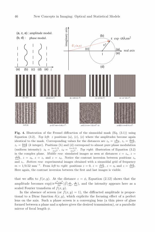
When λzm2 is equal to an integer number k, the amplitude is purely real andequal to 1 ± ε cos(2πmx). When λzm2 = 1/2 + k, the amplitude modulation isan imaginary term, and Uz � 1 ± iε cos(2πmx). For ε very small, the wavefrontis then almost a pure phase factor of uniform amplitude. It can be represented asan undulated wavefront, with advances and delays of the optical path comparedto the plane wave. The wave propagates towards the z direction, continuouslytransforming itself from amplitude to phase modulations, as illustrated in Figure 4.

The observed intensity is

Iz(x, y) ∼ 1 + 2ε cos(2πmx) cos(πλzm2). (3.3)

The fringes almost disappear for z = (k + 1/2)/(λm2), with k integer. Theyare visible with a contrast maximum for z = k/(λm2), and the image is invertedbetween two successive values of k.

At the CNRS school we have also shown the Fresnel diffraction of a Ronchipattern, a two dimensional square wave fR(x, y) made of alternate opaque andtransparent parallel stripes of equal width, as illustrated in Figure 5. Making useof the Fourier series decomposition, we can write the square wave as a simpleaddition of sinusoidal terms of the form:

fR(x, y) =12

+2π

∞∑n=0

12n + 1

sin(2π(2n + 1)mx). (3.4)

The complex amplitude Uz(x, y) at a distance z behind the Ronchi pattern issimply obtained by the sum of the sine terms modified by the transfer function.We have:

Uz(x, y) =12

+2π

∞∑n=0

12n + 1

sin(2π(2n + 1)mx) exp(−iπλz(2n + 1)2m2). (3.5)

As the wave propagates, each sinusoidal component experiences a phase modu-lation depending on its spatial frequency. One obtains an image identical to theRonchi pattern when all the spatial frequencies in Uz(x, y) are phase-shifted by amultiple of 2π. The occurrences of identical images are obtained for λzm2 = 2k,as for the single sine term. This property is known as the Talbot effect.

4 Focusing screens and Fourier transform properties of lenses

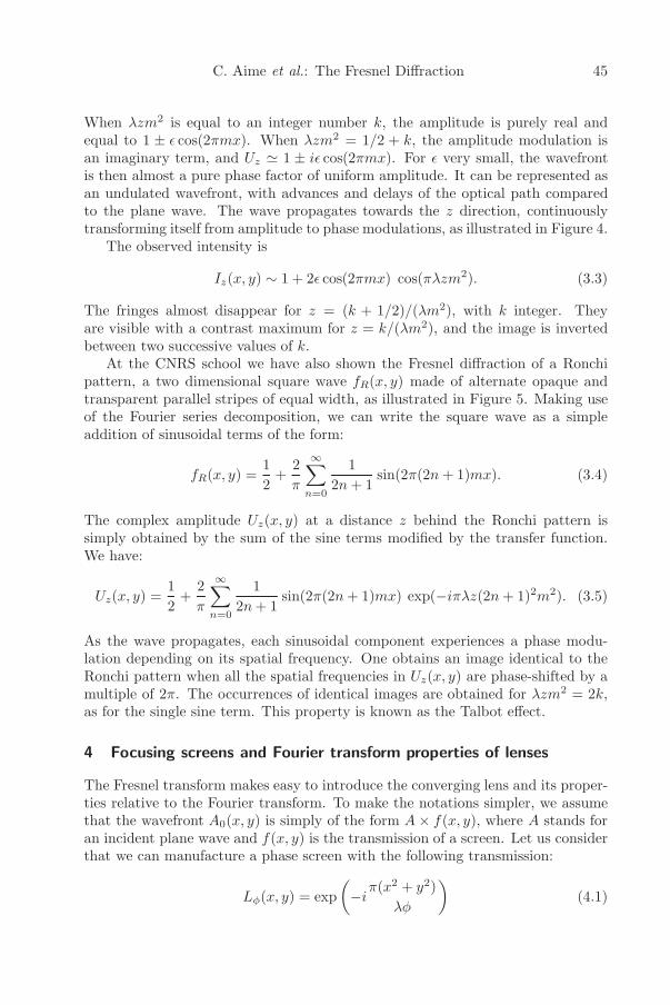
The Fresnel transform makes easy to introduce the converging lens and its proper-ties relative to the Fourier transform. To make the notations simpler, we assumethat the wavefront A0(x, y) is simply of the form A× f(x, y), where A stands foran incident plane wave and f(x, y) is the transmission of a screen. Let us considerthat we can manufacture a phase screen with the following transmission:

Lφ(x, y) = exp(−i

π(x2 + y2)λφ

)(4.1)


1

!axe

imag

inai

re

axe reel

exp -i zm2

(a)

(b)

(c)

(d)

(e)

z (c) (a) (b) (d) (e)

(a, c, e) :

(b, d) : Modul. Amplitude

Modul. Phase

U (x,y)z

phase modul.

real axis

imag

inar

y ax

is

aamplitude modul.

Fig. 4. Illustration of the Fresnel diffraction of the sinusoidal mask (Eq. (3.1)) using

Equation (3.2). Top left: z positions (a), (c), (e) where the amplitudes become again

identical to the mask. Corresponding values for the distances are za = kλm2 , zc = k+1

λm2 ,

ze = k+2λm2 (k integer). Positions (b) and (d) correspond to almost pure phase modulation

(uniform intensity): zb = k+1/2

λm2 , zd = k+3/2

λm2 . Top right: illustration of Equation (3.2)

in the complex plane. Middle row: simulated images as seen at distances z = za, z =1/4

λm2 , z = zb, z = zc and z = zd. Notice the contrast inversion between positions za

and zc. Bottom row: experimental images obtained with a sinusoıdal grid of frequency

m = 1/0.52 mm−1. From left to right: positions z = 0, z = 1/4

λm2 , z = zb and z = 3/4

λm2 .

Here again, the contrast inversion between the first and last images is visible.

that we affix to f(x, y). At the distance z = φ, Equation (2.12) shows that theamplitude becomes exp(iπ x2+y2

λφ )f( xλφ , y

λφ ), and the intensity appears here as ascaled Fourier transform of f(x, y).

In the absence of screen (or f(x, y) = 1), the diffracted amplitude is propor-tional to a Dirac function δ(x, y), which explicits the focusing effect of a perfectlens on the axis. Such a phase screen is a converging lens (a thin piece of glassformed between a plane and a sphere gives the desired transmission), or a parabolicmirror of focal length φ.


Ronchi pattern

Fig. 5. Left: image of a Ronchi pattern. The period if 1/m = 0.86 mm (see Eq. (3.4)).

Top right: optical Fourier tranform of the sinusoidal pattern in the (u, v) plane. Bottom

right: intensity of the optical Fourier transform as a function of the spatial frequency

u for v = 0. Note that the even harmonics of the frequency m are present, while they

should not with a perfect Ronchi pattern with identical widths of white and black strips.

The phase factor exp(iπ x2+y2

λφ ) which remains in this focal plane correspondsto a diverging lens L−φ(x, y). It can be cancelled adding here a converging lens offocal length φ. So, a system made of two identical converging lenses of focal lengthφ separated by a distance φ optically performs the exact Fourier transform of thetransmission in amplitude of a screen. Such a device is called an optical Fouriertransform system. This property becomes obvious if we re-write the Fresnel trans-form of Equation (2.12) making explicit the expression corresponding to diverginglenses:

Az(x, y) =1

iλzL−z(x, y) Fz[A0(x, y)L−z(x, y)]. (4.2)

It is clear here that for the optical Fourier transform system the two converginglenses cancel the diverging terms of propagation. Another similar Fourier trans-form device can be obtained with a single converging lens of focal length φ, settingthe transmission f(x, y) in front of it at the distance φ and observing in its focalplane. Such systems have been used to perform image processing, as described byFrancon (1979).

It is important to note that phase factors disappear also when the quantity ofinterest is the intensity, as for example in incoherent imagery (see Sect. 6). OpticalFourier transforms were actually used in the past to analyse speckle patterns atthe focus of large telescopes (Labeyrie 1970).


4.1 Focusing screens with a real transmission

It is possible to make screens of real transmission (between 0 and 1) acting asconverging lenses. For that, the transmission of the screen must contain a termsimilar to Lφ(x, y). To make its transmission real, we can add the transmission ofa diverging lens L−φ(x, y). Doing so we get a cosine term. It is then necessary toadd a constant term and use the right coefficients to make the transmission of thescreen between 0 and 1. We result in:

sφ(x, y) =12

+14{Lφ(x, y) + L−φ(x, y)} =

12

+12

cos(

π(x2 + y2)λφ

)· (4.3)

Such a screen acts as a converging lens of focal length φ, but with a poor trans-mission (1/4 in amplitude, 1/16 in intensity). It will also act as a diverging lensand as a simple screen of uniform transmission. A different combination of lensesleads to a transmission with a sine term.

The variable transmission of such screens is very difficult to manufacture withprecision. It is easier to make a screen of binary transmission (1 or 0). This canbe done for example by the following transmission:

Sφ(x, y) =12

+2π

∞∑n=0

12n + 1

sin(

π(2n + 1)x2 + y2

λφ

)=

12+

1iπ

∞∑n=0

12n + 1

{exp

(iπ(2n + 1)

x2 + y2

λφ

)− exp

(−iπ(2n + 1)

x2 + y2

λφ

)}

=12

+i

π

∞∑n=0

12n + 1

{Lφ/(2n+1)(x, y)− (L−φ/(2n+1)(x, y)}.

(4.4)

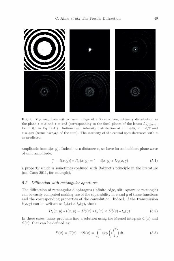
The transmission of such a screen is given in Figure 6 (top left). Its efficiency tofocus in the plane z = φ is slightly improved (from 1/4 to 1/π) at the expense ofan infinite number of converging and diverging lenses (of focal lengths φ/(2n+1)).A few of these ghost focal planes are shown in Figure 6 (experimental results).

These systems may found interesting applications at wavelengths for whichit is difficult to manufacture classical lenses or mirrors. It is interesting to notethat screens based on this principle have been proposed also for astronomicalapplications in the visible domain by Koechlin et al. (2009).

5 Fresnel diffraction and shadowing in astronomy: Applicationto coronagraphy

5.1 Fresnel diffraction with complementary screens

Let us consider two complementary screens of the form t(x, y) and 1 − t(x, y).The amplitude diffracted by the complementary screen is 1 minus the diffracted


Fig. 6. Top row, from left to right: image of a Soret screen, intensity distribution in

the plane z = φ and z = φ/3 (corresponding to the focal planes of the lenses Lφ/(2n+1)

for n=0,1 in Eq. (4.4)). Bottom row: intensity distribution at z = φ/5, z = φ/7 and

z = φ/9 (terms n=2,3,4 of the sum). The intensity of the central spot decreases with n

as predicted.

amplitude from t(x, y). Indeed, at a distance z, we have for an incident plane waveof unit amplitude:

(1− t(x, y)) ∗Dz(x, y) = 1− t(x, y) ∗Dz(x, y) (5.1)

a property which is sometimes confused with Babinet’s principle in the literature(see Cash 2011, for example).

5.2 Diffraction with rectangular apertures

The diffraction of rectangular diaphragms (infinite edge, slit, square or rectangle)can be easily computed making use of the separability in x and y of these functionsand the corresponding properties of the convolution. Indeed, if the transmissiont(x, y) can be written as tx(x)× ty(y), then:

Dz(x, y) ∗ t(x, y) = D0z(x) ∗ tx(x) ×D0

z(y) ∗ ty(y). (5.2)

In these cases, many problems find a solution using the Fresnel integrals C(x) andS(x), that can be defined as:

F (x) = C(x) + iS(x) =∫ x

0

exp(

it2

2

)dt. (5.3)


2 1 0 1 2 3 40.0

0.2

0.4

0.6

0.8

1.0

1.2

1.4

2 1 0 1 2 3 40

2 Π

4 Π

6 Π

Fig. 7. Left: normalized intensity and right: phase (unwrapped) of the Fresnel diffraction

of an infinite edge H(x), outlined in the left figure. The observing plane is at 1 m from

the screen, the wavelength is 0.6 μm. The x-axis is in mm.

The complex amplitude diffracted by an edge is obtained computing the convolu-tion of Dz(x, y) with the Heaviside function H(x) for all x and y (we may denoteits transmission as t(x, y) = H(x)× 1(y) for clarity). We have:

AH(x, y) = Dz(x, y) ∗H(x) = D0z(x) ∗H(x) =

12

+1√2i

F

(x

√2zλ

)· (5.4)

The intensity and the phase of the wave are given in Figure 7. The intensity isvery often represented in Fresnel diffraction, but this is not the case for the phase.The rapid increase of phase in the geometrical dark zone may be heuristicallyinterpreted as a tilted wavefront, the light coming there originating from the brightzone.

Similarly, the free space propagation of the light for a slit of width L canbe directly derived from the above relation assuming that the transmission ist(x, y) = H(x + L/2)−H(x− L/2). We have:

AL+(x, y) =1√2i

{F (

2x + L√2λz

)− F (2x− L√

2λz)}

(5.5)

where the subscript L+ stands for a clear slit of width L. Graphical representationsof the corresponding intensity and phase are displayed in Figure 8.

As already written, the Fresnel diffracted amplitude from the complementaryscreen can be obtained as 1 minus the diffracted amplitude from the slit. It canbe also be written as the sum of the diffraction of two bright edges H(x − L/2)and H(−x − L/2). Then it is clear that ripples visible in the shadow of the slitare due to phase terms produced by the edges. We have:

AL−(x, y) = 1− 1√2i

{F

(2x + L√

2λz

)+ F

(2x− L√

2λz

)}=

1√2i

F

(−2x− L√2λz

)+

1√2i

F

(2x− L√

2λz

)(5.6)

where L− stands for an opaque strip of width L.


1.0 0.5 0.0 0.5 1.00.0

0.5

1.0

1.5

1.0 0.5 0.0 0.5 1.00.0

0.5

1.0

1.5

Fig. 8. Fresnel diffractions (in intensity) of a transmitting slit (left) and an opaque slit

(right) of width 1 mm (slits are outlined in the figures). Observing planes are at 0.3 m

(red), 1 m (blue) and 3 m (dashed) from the screen, the wavelength is 0.6 μm.

Fig. 9. Fresnel diffraction (left: amplitude, right: phase) of a square occulter of side 50 m

at 80 000 km, with λ = 0.6 μm. The region represented in the figures is 100 m × 100 m.

The color scale for the amplitude (black, white, blue, red) is chosen so as to highlight the

structures in the dark zone of the screen. The color scale for the phase is blue for −π,

black for 0 and red for +π (the phase is not unwrapped here).

A transmitting square (or rectangle) aperture can be written as the prod-uct of two orthogonal slits. Therefore the Fresnel diffraction of the open squareAL2+(x, y) is the combination of two Fresnel diffractions in x and y. This prop-erty of separability is no longer verified for the diffraction of the opaque squareAL2−(x, y), which transmission must be written as 1 minus the transmission ofthe open square. We have:

AL2+(x, y) =ALx+(x, y)×ALy+(x, y)AL2−(x, y) =1−AL2+(x, y). (5.7)

We give in Figure 9 an example of the amplitude and phase of the wave in theshadow of a square occulter of 50×50 meters at a distance of 80 000 km, and that


could possibly be used for exoplanet detection. These parameters are compatiblewith the observation of a planet at about 0.1 arcsec from the star (a Solar – Earthsystem at 10 parsec) with a 4-m telescope. It is however interesting to note thestrong phase perturbation in the center of the shadow, while it is almost zerooutside. In such an experiment, the telescope is set in the center of the pattern toblock the direct starlight, and the planet is observable beyond the angular darkzone of the occulter. The level of intensity in the central zone is of the order of10−4 of that of the direct light. This is still too bright to perform direct detectionof exoplanets: the required value is 10−6 or less. To make the shadow darker itwould be necessary to increase the size of the occulter and the distance betweenthe occulter and the telescope.

5.3 Fresnel diffraction with a circular occulter: The Arago-Poisson spot

The transmission of a circular occulter of diameter D can be written as 1−Π(r/D),where r =

√x2 + y2, and Π(r) is the rectangle function of transmission 1 for

|r| < 1/2 and 0 elsewhere. Since the occulter is a radial function, its Fresneldiffraction is also a radial function that can be written as:

AD(r) = 1− 1iλz

exp(

iπr2

λz

)∫ D/2

0

2πξ exp(

iπξ2

λz

)J0

(2π

ξr

λz

)dξ (5.8)

where J0(r) is the Bessel function of the first kind. Here again, the Fresnel diffrac-tion from the occulter writes as 1 minus the Fresnel diffraction of the hole. At thecenter of the shadow we have AD(0) = exp[iπD2/(4λz)] and we recover the valueof 1 for the intensity.

Obtaining the complete expression of the wave for any r value is somewhattricky. The integral of Equation (5.8) is a Hankel transform that does not have asimple analytic solution. A similar problem (the wave amplitude near the focusof a lens) has been solved by Lommel, as described by Born & Wolf (2006). Itis possible to transpose their approach to obtain the Fresnel diffraction from acircular occulter.

After a lot of calculations, we obtain the result in the form of alternatingLommel series for the real and imaginary parts of the amplitude. The result canbe represented in a concise form as:

Ψ(r) =

r < D/2 : A exp(

iπr2

λz

)exp

(iπD2

4λz

)×

∞∑k=0

(−i)k

(2r

D

)k

Jk

(πDr

λz

)r = D/2 :

A

2

[1 + exp

(iπD2

2λz

)J0

(πD2

2λz

)]r > D/2 : A−A exp

(iπr2

λz

)exp

(iπD2

4λz

)×

∞∑k=1

(−i)k

(D

2r

)k

Jk

(πDr

λz

)·

(5.9)


Two expressions are needed to ensure the convergence of the sum depending onthe value of 2r/D compared to 1. The convergence is fast except for the transitionzone around r ∼ D/2, and luckily there is a simple analytical form there. Anupper bound of the series limited to n terms is given by the absolute value of then + 1 term, according to Leibniz’ estimate.

An illustration of this formula is given in Figure 10 for an occulter of diameter50 m, observed at a distance of 80 000 km, at λ = 0.55 μm, which corresponds todata for the exoplanet case. For this figure, we computed the series for 100 terms,which can be rapidly done using Mathematica (Wolfram 2012) and gives a suffi-cient precision everywhere. The Arago spot is clearly visible at the center of thediffraction zone. For r � D, the amplitude is fairly described by the only non-zeroterm of the Lommel series that is the Bessel function J0(πrD/(λz)). Its diameteris approximately 1.53λz/D.

As mentioned in the introduction, Arago’s experience was reproduced duringthe CNRS school of June 2012. Fresnel diffraction patterns (intensity) of a smallocculter, reproduced in Figure 1 show the Arago spot at their center.

Thus a circular screen is not a good occulter.For the detection of exoplanets, several projects envisage petaled occulters

(Arenberg et al. 2007; Cash 2011) and we give an illustration of the performancesin Figure 11. The analytic study of circular occulters remains however of interestfor solar applications. Indeed, because of the extended nature of the solar disk, itseems difficult to use shaped occulters there, even if serrated edge occulters havebeen envisaged for that application (Koutchmy 1988).

Out[89]=40 20 0 20 40

0.0

0.2

0.4

0.6

0.8

1.0

1.2

40 20 0 20 400

10

20

30

40

Fig. 10. Fresnel diffraction of an occulter of diameter 50 m, observed at a distance of

80 000 km, at λ = 0.55 μm. Left: 2D intensity, top right: central cut of the intensity,

bottom right: central cut of the unwrapped phase. Notice the strong Arago spot at the

center of the shadow and the important phase variation.


Fig. 11. Fresnel diffraction of an occulter with a petal shape. From left to right: the

occulter, the intensity (×10) in the shadow and the phase. The parameters are the same

as in Figure 10 D = 50 m, z = 80 000 km, λ = 0.55 μm. The shadow at the center of the

screen is much darker (no Arago spot) and the phase variation is weak there.

Fig. 12. Numerical 3D representation of the PSF (left), here an Airy function, and the

corresponding OTF (right) of a perfect telescope with a circular entrance aperture.

6 Application to incoherent imaging in astronomy

The formation of an image at the focus of a telescope in astronomy can be di-vided into two steps, one corresponding to a coherent process leading to the pointspread function (PSF) and the other corresponding to a sum of intensities, e.g. anincoherent process. Equation (4.2) makes it possible to write the PSF observedin the focal plane of the telescope as a function of the spatial (x, y) or angular(α = x/φ, β = y/φ) coordinates. For an on-axis point-source of unit intensity, wehave:

Rφ(x, y) =1

Sλ2φ2

∣∣∣∣P (x

λφ,

y

λφ

)∣∣∣∣2R(α, β) =

1Sλ2

∣∣∣∣P (α

λ,β

λ

)∣∣∣∣2 (6.1)

where φ is the telescope focal length and P (x, y) is the function that defines thetelescope transmission. Aberrations or other phase defaults due to atmosphericturbulence can be included in the term P (x, y). The division by the surface area


Fig. 13. Example of PSFs shown during the CNRS school using a simple optical setup.

Top, circular apertures, bottom, corresponding PSFs. Note the inverse relationship be-

tween the size of the PSF and the aperture diameter.

S of the telescope allows the calculation of a normalized PSF. The normalizingcoefficients ensure the energy conservation of the form:∫∫

Rφ(x, y) dxdy =∫∫

R(α, β) dαdβ =1S

∫∫|P (ξ, η)|2 dξdη = 1. (6.2)

We have made use of Parseval theorem to write the last equality. For a telescopeof variable transmission, see Aime (2005).

It is convenient to consider angular coordinates independent of the focal lengthof the instrument. Each point of the object forms its own response in intensityshifted at the position corresponding to its angular location. This leads to aconvolution relationship. The focal plane image is reversed compared to the objectsense. By orienting the axes in the focal plane in the same direction as in the sky,


Fig. 14. From left to right: aperture, PSF and MTF. For the sake of clarity, the MTF

corresponding to the 18-aperture interferometer is drawn for smaller elementary apertures

than those of the left figure.

we obtain:

I(α, β) = O(α, β) ∗R(−α,−β) (6.3)


where O(α, β) is the irradiance of the astronomical object. The Fourier transformof R(−α,−β) gives the optical transfer function (OTF) T (u, v):

T (u, v) = F [R(−α,−β)] =1S

∫ ∫P (x, y)P ∗(x− λu, y − λv)dxdy (6.4)

where u and v are the angular spatial frequencies.For a perfect circular aperture of diameter D operated at the wavelength λ,

the PSF becomes the following radial function of γ:

R(α, β) = R(γ) =(

2J1(πγD/λ)

πγD/λ

)2S2

λ2(6.5)

where γ =√

α2 + β2, and the OTF is the radial function of w =√

u2 + v2:

T (u, v) = T(w) =2π

⎛⎝arccos(

λw

D

)− λw

D

√1−

(λw

D

)2⎞⎠ · (6.6)

This expression is obtained computing the surface common to two shifted discs.The OTF looks like a Chinese-hat, with a high frequency cutoff wc = D/λ.

Examples of PSFs for various apertures presented during the CNRS schoolare given in Figure 14. The corresponding MTFs shown in the same figure arecomputed numerically.

7 Conclusion

This presentation aimed at introducing the formalism for Fresnel’s diffraction the-ory, widely used in optics and astronomy.

Besides analytical derivation of basic relationships involving instrumental pa-rameters, visual illustrations using laboratory demonstrations are given, as waspresented during the CNRS school. Most of these are basic in the field of imageformation and are frequently met in astronomy. A few of them concerning theshadows produced by the screens are seldomly addressed in the astronomical lit-erature up to now, though they presently are emerging topics. Demonstrationsare made using laboratory material for students in Physics: a laser and a beamexpander, various transmitting or opaque screens and a detector.

The paper begins with a historical background leading to the current context.Then analytical derivations, based on the Huyghens-Fresnel principle, using wave-fronts and complex amplitudes are presented, providing expressions for the freespace propagation of light. Plenty use is made of convolution relationships andfiltering aspects.

Fresnel’s diffraction is illustrated through some situations, such as the propa-gation after a screen with sinusoidal transmission function, or such as shadowingproduced by occulters set on the pointing direction of a telescope for coronagra-phy. Here are met such effects as the so-called Poisson-Arago spot, and diffraction


by sharp edges (rectangular or circular screens). The use of focusing screens havebeen considered as well. Along that way, expressions of diffracted amplitudes aregiven for various shapes of apertures. Then, the Fourier transform properties oflenses and binary screens (made of transparent and opaque zones, i.e. transmissionfunction being 0 or 1 accordingly) are presented.

The paper ends with a section describing incoherent imaging in astronomy anddealing with PSFs (intensity response of the instrument to a point-like source)and MTFs (a link with linear filtering). Images of PSFs obtained with the demon-stration set-up, are presented for various shapes and configurations of collectingapertures: from single disk to diluted apertures (several sub-pupils) as used inaperture synthesis with several telescopes. Besides, illustrations for associatedMTFs are obtained by computation.

The paper could hopefully be used either as a reminder or as an introductionto the basics of the image formation process in the context of diffraction theory.

The authors wish to thank Dr S. Robbe-Dubois for her critical reading of the manuscript.

References

Aime, C., 2005, A&A, 434, 785

Arenberg, J.W., Lo, A.S., Glassman, T.M., & Cash, W., 2007, C.R. Physique, 8, 438

Born, M., & Wolf, E., 2006, Principles of Optics, 7th Ed. (Cambridge University Press),484

Cash, W., 2011, ApJ, 738, 76

Koechlin, L., Serre, D., & Deba, P., 2009, Ap&SS, 320, 225

Francon, M., 1979, Optical image formation and processing (New York: Academic Press)

Goodman, J.W., 1985, Statistical Optics (New York, NY: John Wiley and Sons)

Goodman, J.W., 2005, Introduction to Fourier Optics (Roberts and Company Publishers)

Koutchmy, S., 1988, Space Sci. Rev., 47, 95

Labeyrie, A., 1970, A&A, 6, 85

Lamy, P., Dame, L., Vives, S., & Zhukov, A., 2010, SPIE, 7731, 18

Nazarathy, M., & Shamir, J., 1980, J. Opt. Soc. Am., 70, 150

de Senarmont, M., Verdet, E., & Fresnel, L., 1866, Oeuvres completes d’Augustin Fresnel(Paris, Imprimerie Imperiale)

Wolfram Mathematica, 2012, Wolfram Research, Inc., Champaign, IL

THE FRESNEL DIFFRACTION: A STORY OF LIGHT AND … · THE FRESNEL DIFFRACTION: A STORY OF LIGHT AND...

Documents

Transcript of THE FRESNEL DIFFRACTION: A STORY OF LIGHT AND … · THE FRESNEL DIFFRACTION: A STORY OF LIGHT AND...