The FREQ Procedure - SAS Support
207
SAS/STAT ® 13.1 User’s Guide The FREQ Procedure
Transcript of The FREQ Procedure - SAS Support

SAS/STAT® 13.1 User’s GuideThe FREQ Procedure

This document is an individual chapter from SAS/STAT® 13.1 User’s Guide.
The correct bibliographic citation for the complete manual is as follows: SAS Institute Inc. 2013. SAS/STAT® 13.1 User’s Guide.Cary, NC: SAS Institute Inc.
Copyright © 2013, SAS Institute Inc., Cary, NC, USA
All rights reserved. Produced in the United States of America.
For a hard-copy book: No part of this publication may be reproduced, stored in a retrieval system, or transmitted, in any form or byany means, electronic, mechanical, photocopying, or otherwise, without the prior written permission of the publisher, SAS InstituteInc.
For a web download or e-book: Your use of this publication shall be governed by the terms established by the vendor at the timeyou acquire this publication.
The scanning, uploading, and distribution of this book via the Internet or any other means without the permission of the publisher isillegal and punishable by law. Please purchase only authorized electronic editions and do not participate in or encourage electronicpiracy of copyrighted materials. Your support of others’ rights is appreciated.
U.S. Government License Rights; Restricted Rights: The Software and its documentation is commercial computer softwaredeveloped at private expense and is provided with RESTRICTED RIGHTS to the United States Government. Use, duplication ordisclosure of the Software by the United States Government is subject to the license terms of this Agreement pursuant to, asapplicable, FAR 12.212, DFAR 227.7202-1(a), DFAR 227.7202-3(a) and DFAR 227.7202-4 and, to the extent required under U.S.federal law, the minimum restricted rights as set out in FAR 52.227-19 (DEC 2007). If FAR 52.227-19 is applicable, this provisionserves as notice under clause (c) thereof and no other notice is required to be affixed to the Software or documentation. TheGovernment’s rights in Software and documentation shall be only those set forth in this Agreement.
SAS Institute Inc., SAS Campus Drive, Cary, North Carolina 27513-2414.
December 2013
SAS provides a complete selection of books and electronic products to help customers use SAS® software to its fullest potential. Formore information about our offerings, visit support.sas.com/bookstore or call 1-800-727-3228.
SAS® and all other SAS Institute Inc. product or service names are registered trademarks or trademarks of SAS Institute Inc. in theUSA and other countries. ® indicates USA registration.
Other brand and product names are trademarks of their respective companies.

SAS and all other SAS Institute Inc. product or service names are registered trademarks or trademarks of SAS Institute Inc. in the USA and other countries. ® indicates USA registration. Other brand and product names are trademarks of their respective companies. © 2013 SAS Institute Inc. All rights reserved. S107969US.0613
Discover all that you need on your journey to knowledge and empowerment.
support.sas.com/bookstorefor additional books and resources.
Gain Greater Insight into Your SAS® Software with SAS Books.

Chapter 40
The FREQ Procedure
ContentsOverview: FREQ Procedure . . . . . . . . . . . . . . . . . . . . . . . . . . . . . . . . . . 2622Getting Started: FREQ Procedure . . . . . . . . . . . . . . . . . . . . . . . . . . . . . . . 2624
Frequency Tables and Statistics . . . . . . . . . . . . . . . . . . . . . . . . . . . . . 2624Agreement Study . . . . . . . . . . . . . . . . . . . . . . . . . . . . . . . . . . . . . 2631
Syntax: FREQ Procedure . . . . . . . . . . . . . . . . . . . . . . . . . . . . . . . . . . . . 2634PROC FREQ Statement . . . . . . . . . . . . . . . . . . . . . . . . . . . . . . . . . 2634BY Statement . . . . . . . . . . . . . . . . . . . . . . . . . . . . . . . . . . . . . . 2636EXACT Statement . . . . . . . . . . . . . . . . . . . . . . . . . . . . . . . . . . . . 2637OUTPUT Statement . . . . . . . . . . . . . . . . . . . . . . . . . . . . . . . . . . . 2645TABLES Statement . . . . . . . . . . . . . . . . . . . . . . . . . . . . . . . . . . . 2656TEST Statement . . . . . . . . . . . . . . . . . . . . . . . . . . . . . . . . . . . . . 2693WEIGHT Statement . . . . . . . . . . . . . . . . . . . . . . . . . . . . . . . . . . . 2696
Details: FREQ Procedure . . . . . . . . . . . . . . . . . . . . . . . . . . . . . . . . . . . . 2697Inputting Frequency Counts . . . . . . . . . . . . . . . . . . . . . . . . . . . . . . . 2697Grouping with Formats . . . . . . . . . . . . . . . . . . . . . . . . . . . . . . . . . 2698Missing Values . . . . . . . . . . . . . . . . . . . . . . . . . . . . . . . . . . . . . . 2699In-Database Computation . . . . . . . . . . . . . . . . . . . . . . . . . . . . . . . . 2701Statistical Computations . . . . . . . . . . . . . . . . . . . . . . . . . . . . . . . . . 2702
Definitions and Notation . . . . . . . . . . . . . . . . . . . . . . . . . . . . 2702Chi-Square Tests and Statistics . . . . . . . . . . . . . . . . . . . . . . . . . 2704Measures of Association . . . . . . . . . . . . . . . . . . . . . . . . . . . . 2709Binomial Proportion . . . . . . . . . . . . . . . . . . . . . . . . . . . . . . 2719Risks and Risk Differences . . . . . . . . . . . . . . . . . . . . . . . . . . . 2725Common Risk Difference . . . . . . . . . . . . . . . . . . . . . . . . . . . . 2736Odds Ratio and Relative Risks for 2 x 2 Tables . . . . . . . . . . . . . . . . 2737Cochran-Armitage Test for Trend . . . . . . . . . . . . . . . . . . . . . . . 2740Jonckheere-Terpstra Test . . . . . . . . . . . . . . . . . . . . . . . . . . . . 2741Tests and Measures of Agreement . . . . . . . . . . . . . . . . . . . . . . . 2743Cochran-Mantel-Haenszel Statistics . . . . . . . . . . . . . . . . . . . . . . 2748Gail-Simon Test for Qualitative Interactions . . . . . . . . . . . . . . . . . . 2756Exact Statistics . . . . . . . . . . . . . . . . . . . . . . . . . . . . . . . . . 2757
Computational Resources . . . . . . . . . . . . . . . . . . . . . . . . . . . . . . . . 2761Output Data Sets . . . . . . . . . . . . . . . . . . . . . . . . . . . . . . . . . . . . . 2762Displayed Output . . . . . . . . . . . . . . . . . . . . . . . . . . . . . . . . . . . . . 2765ODS Table Names . . . . . . . . . . . . . . . . . . . . . . . . . . . . . . . . . . . . 2773ODS Graphics . . . . . . . . . . . . . . . . . . . . . . . . . . . . . . . . . . . . . . 2777

2622 F Chapter 40: The FREQ Procedure
Examples: FREQ Procedure . . . . . . . . . . . . . . . . . . . . . . . . . . . . . . . . . . 2778Example 40.1: Output Data Set of Frequencies . . . . . . . . . . . . . . . . . . . . . 2778Example 40.2: Frequency Dot Plots . . . . . . . . . . . . . . . . . . . . . . . . . . . 2781Example 40.3: Chi-Square Goodness-of-Fit Tests . . . . . . . . . . . . . . . . . . . 2784Example 40.4: Binomial Proportions . . . . . . . . . . . . . . . . . . . . . . . . . . 2788Example 40.5: Analysis of a 2x2 Contingency Table . . . . . . . . . . . . . . . . . . 2791Example 40.6: Output Data Set of Chi-Square Statistics . . . . . . . . . . . . . . . . 2794Example 40.7: Cochran-Mantel-Haenszel Statistics . . . . . . . . . . . . . . . . . . 2796Example 40.8: Cochran-Armitage Trend Test . . . . . . . . . . . . . . . . . . . . . . 2798Example 40.9: Friedman’s Chi-Square Test . . . . . . . . . . . . . . . . . . . . . . . 2802Example 40.10: Cochran’s Q Test . . . . . . . . . . . . . . . . . . . . . . . . . . . . 2803
References . . . . . . . . . . . . . . . . . . . . . . . . . . . . . . . . . . . . . . . . . . . 2806
Overview: FREQ ProcedureThe FREQ procedure produces one-way to n-way frequency and contingency (crosstabulation) tables. Fortwo-way tables, PROC FREQ computes tests and measures of association. For n-way tables, PROC FREQprovides stratified analysis by computing statistics across, as well as within, strata.
For one-way frequency tables, PROC FREQ computes goodness-of-fit tests for equal proportions or specifiednull proportions. For one-way tables, PROC FREQ also provides confidence limits and tests for binomialproportions, including tests for noninferiority and equivalence.
For contingency tables, PROC FREQ can compute various statistics to examine the relationships betweentwo classification variables. For some pairs of variables, you might want to examine the existence or strengthof any association between the variables. To determine if an association exists, chi-square tests are computed.To estimate the strength of an association, PROC FREQ computes measures of association that tend to beclose to zero when there is no association and close to the maximum (or minimum) value when there isperfect association. The statistics for contingency tables include the following:
• chi-square tests and measures
• measures of association
• risks (binomial proportions) and risk differences for 2 � 2 tables
• odds ratios and relative risks for 2 � 2 tables
• tests for trend
• tests and measures of agreement
• Cochran-Mantel-Haenszel statistics

Overview: FREQ Procedure F 2623
PROC FREQ computes asymptotic standard errors, confidence intervals, and tests for measures of associationand measures of agreement. Exact p-values and confidence intervals are available for many test statisticsand measures. PROC FREQ also performs analyses that adjust for any stratification variables by computingstatistics across, as well as within, strata for n-way tables. These statistics include Cochran-Mantel-Haenszelstatistics and measures of agreement.
In choosing measures of association to use in analyzing a two-way table, you should consider the study design(which indicates whether the row and column variables are dependent or independent), the measurementscale of the variables (nominal, ordinal, or interval), the type of association that each measure is designedto detect, and any assumptions required for valid interpretation of a measure. You should exercise care inselecting measures that are appropriate for your data.
Similar comments apply to the choice and interpretation of test statistics. For example, the Mantel-Haenszelchi-square statistic requires an ordinal scale for both variables and is designed to detect a linear association.The Pearson chi-square, on the other hand, is appropriate for all variables and can detect any kind ofassociation, but it is less powerful for detecting a linear association because its power is dispersed over agreater number of degrees of freedom (except for 2 � 2 tables).
For more information about selecting the appropriate statistical analyses, see Agresti (2007) and Stokes,Davis, and Koch (2012).
Several SAS procedures produce frequency counts; only PROC FREQ computes chi-square tests for one-wayto n-way tables and measures of association and agreement for contingency tables. Other procedures toconsider for counting include the TABULATE and UNIVARIATE procedures. When you want to producecontingency tables and tests of association for sample survey data, use PROC SURVEYFREQ. See Chapter 14,“Introduction to Survey Procedures,” for more information. When you want to fit models to categorical data,use a procedure such as CATMOD, GENMOD, GLIMMIX, LOGISTIC, PROBIT, or SURVEYLOGISTIC.See Chapter 8, “Introduction to Categorical Data Analysis Procedures,” for more information.
PROC FREQ uses the Output Delivery System (ODS), a SAS subsystem that provides capabilities fordisplaying and controlling the output from SAS procedures. ODS enables you to convert any of the outputfrom PROC FREQ into a SAS data set. See the section “ODS Table Names” on page 2773 for moreinformation.
PROC FREQ uses ODS Graphics to create graphs as part of its output. For general information about ODSGraphics, see Chapter 21, “Statistical Graphics Using ODS.” For specific information about the statisticalgraphics available with the FREQ procedure, see the PLOTS= option in the TABLES statement and thesection “ODS Graphics” on page 2777.

2624 F Chapter 40: The FREQ Procedure
Getting Started: FREQ Procedure
Frequency Tables and StatisticsThe FREQ procedure provides easy access to statistics for testing for association in a crosstabulation table.
In this example, high school students applied for courses in a summer enrichment program; these coursesincluded journalism, art history, statistics, graphic arts, and computer programming. The students acceptedwere randomly assigned to classes with and without internships in local companies. Table 40.1 containscounts of the students who enrolled in the summer program by gender and whether they were assigned aninternship slot.
Table 40.1 Summer Enrichment Data
EnrollmentGender Internship Yes No Totalboys yes 35 29 64boys no 14 27 41girls yes 32 10 42girls no 53 23 76
The SAS data set SummerSchool is created by inputting the summer enrichment data as cell count data, orproviding the frequency count for each combination of variable values. The following DATA step statementscreate the SAS data set SummerSchool:
data SummerSchool;input Gender $ Internship $ Enrollment $ Count @@;datalines;
boys yes yes 35 boys yes no 29boys no yes 14 boys no no 27girls yes yes 32 girls yes no 10girls no yes 53 girls no no 23;
The variable Gender takes the values ‘boys’ or ‘girls,’ the variable Internship takes the values ‘yes’ and‘no,’ and the variable Enrollment takes the values ‘yes’ and ‘no.’ The variable Count contains the number ofstudents that correspond to each combination of data values. The double at sign (@@) indicates that morethan one observation is included on a single data line. In this DATA step, two observations are included oneach line.
Researchers are interested in whether there is an association between internship status and summer programenrollment. The Pearson chi-square statistic is an appropriate statistic to assess the association in thecorresponding 2 � 2 table. The following PROC FREQ statements specify this analysis.
You specify the table for which you want to compute statistics with the TABLES statement. You specify thestatistics you want to compute with options after a slash (/) in the TABLES statement.
Frequency Tables and Statistics F 2625
proc freq data=SummerSchool order=data;tables Internship*Enrollment / chisq;weight Count;
run;
The ORDER= option controls the order in which variable values are displayed in the rows and columnsof the table. By default, the values are arranged according to the alphanumeric order of their unformattedvalues. If you specify ORDER=DATA, the data are displayed in the same order as they occur in the inputdata set. Here, because ‘yes’ appears before ‘no’ in the data, ‘yes’ appears first in any table. Other optionsfor controlling order include ORDER=FORMATTED, which orders according to the formatted values, andORDER=FREQUENCY, which orders by descending frequency count.
In the TABLES statement, Internship*Enrollment specifies a table where the rows are internship status and thecolumns are program enrollment. The CHISQ option requests chi-square statistics for assessing associationbetween these two variables. Because the input data are in cell count form, the WEIGHT statement is required.The WEIGHT statement names the variable Count, which provides the frequency of each combination ofdata values.
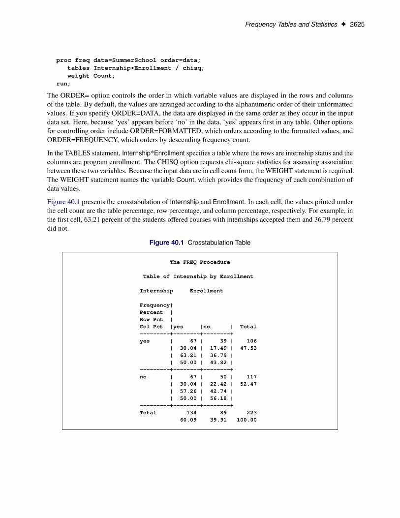
Figure 40.1 presents the crosstabulation of Internship and Enrollment. In each cell, the values printed underthe cell count are the table percentage, row percentage, and column percentage, respectively. For example, inthe first cell, 63.21 percent of the students offered courses with internships accepted them and 36.79 percentdid not.
Figure 40.1 Crosstabulation Table
The FREQ Procedure
Table of Internship by Enrollment
Internship Enrollment
Frequency|Percent |Row Pct |Col Pct |yes |no | Total---------+--------+--------+yes | 67 | 39 | 106
| 30.04 | 17.49 | 47.53| 63.21 | 36.79 || 50.00 | 43.82 |
---------+--------+--------+no | 67 | 50 | 117
| 30.04 | 22.42 | 52.47| 57.26 | 42.74 || 50.00 | 56.18 |
---------+--------+--------+Total 134 89 223
60.09 39.91 100.00

2626 F Chapter 40: The FREQ Procedure
Figure 40.2 displays the statistics produced by the CHISQ option. The Pearson chi-square statistic is labeled‘Chi-Square’ and has a value of 0.8189 with 1 degree of freedom. The associated p-value is 0.3655, whichmeans that there is no significant evidence of an association between internship status and program enrollment.The other chi-square statistics have similar values and are asymptotically equivalent. The other statistics (phicoefficient, contingency coefficient, and Cramér’s V) are measures of association derived from the Pearsonchi-square. For Fisher’s exact test, the two-sided p-value is 0.4122, which also shows no association betweeninternship status and program enrollment.
Figure 40.2 Statistics Produced with the CHISQ Option
Statistic DF Value Prob------------------------------------------------------Chi-Square 1 0.8189 0.3655Likelihood Ratio Chi-Square 1 0.8202 0.3651Continuity Adj. Chi-Square 1 0.5899 0.4425Mantel-Haenszel Chi-Square 1 0.8153 0.3666Phi Coefficient 0.0606Contingency Coefficient 0.0605Cramer's V 0.0606
Fisher's Exact Test----------------------------------Cell (1,1) Frequency (F) 67Left-sided Pr <= F 0.8513Right-sided Pr >= F 0.2213
Table Probability (P) 0.0726Two-sided Pr <= P 0.4122
The analysis, so far, has ignored gender. However, it might be of interest to ask whether program enrollmentis associated with internship status after adjusting for gender. You can address this question by doing ananalysis of a set of tables (in this case, by analyzing the set consisting of one for boys and one for girls). TheCochran-Mantel-Haenszel (CMH) statistic is appropriate for this situation: it addresses whether rows andcolumns are associated after controlling for the stratification variable. In this case, you would be stratifyingby gender.
The PROC FREQ statements for this analysis are very similar to those for the first analysis, except that thereis a third variable, Gender, in the TABLES statement. When you cross more than two variables, the tworightmost variables construct the rows and columns of the table, respectively, and the leftmost variablesdetermine the stratification.
The following PROC FREQ statements also request frequency plots for the crosstabulation tables. PROCFREQ produces these plots by using ODS Graphics to create graphs as part of the procedure output.ODS Graphics must be enabled before producing plots. The PLOTS(ONLY)=FREQPLOT option requestsfrequency plots. The TWOWAY=CLUSTER plot-option specifies a cluster layout for the two-way frequencyplots.

Frequency Tables and Statistics F 2627
ods graphics on;proc freq data=SummerSchool;
tables Gender*Internship*Enrollment /chisq cmh plots(only)=freqplot(twoway=cluster);
weight Count;run;ods graphics off;
This execution of PROC FREQ first produces two individual crosstabulation tables of Internship byEnrollment: one for boys and one for girls. Frequency plots and chi-square statistics are produced foreach individual table. Figure 40.3, Figure 40.4, and Figure 40.5 show the results for boys. Note that thechi-square statistic for boys is significant at the ˛ D 0:05 level of significance. Boys offered a course with aninternship are more likely to enroll than boys who are not.
Figure 40.4 displays the frequency plot of Internship by Enrollment for boys. By default, frequency plots aredisplayed as bar charts. You can use PLOTS= options to request dot plots instead of bar charts, to changethe orientation of the bars from vertical to horizontal, and to change the scale from frequencies to percents.You can also use PLOTS= options to specify other two-way layouts (stacked, vertical groups, or horizontalgroups) and to change the primary grouping from column levels to row levels.
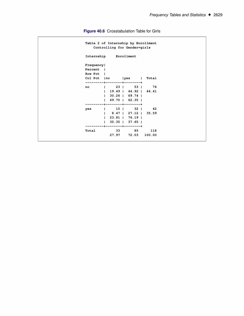
Figure 40.6, Figure 40.7, and Figure 40.8 display the crosstabulation table, frequency plot, and chi-squarestatistics for girls. You can see that there is no evidence of association between internship offers and programenrollment for girls.
Figure 40.3 Crosstabulation Table for Boys
The FREQ Procedure
Table 1 of Internship by EnrollmentControlling for Gender=boys
Internship Enrollment
Frequency|Percent |Row Pct |Col Pct |no |yes | Total---------+--------+--------+no | 27 | 14 | 41
| 25.71 | 13.33 | 39.05| 65.85 | 34.15 || 48.21 | 28.57 |
---------+--------+--------+yes | 29 | 35 | 64
| 27.62 | 33.33 | 60.95| 45.31 | 54.69 || 51.79 | 71.43 |
---------+--------+--------+Total 56 49 105
53.33 46.67 100.00

2628 F Chapter 40: The FREQ Procedure
Figure 40.4 Frequency Plot for Boys
Figure 40.5 Chi-Square Statistics for Boys
Statistic DF Value Prob------------------------------------------------------Chi-Square 1 4.2366 0.0396Likelihood Ratio Chi-Square 1 4.2903 0.0383Continuity Adj. Chi-Square 1 3.4515 0.0632Mantel-Haenszel Chi-Square 1 4.1963 0.0405Phi Coefficient 0.2009Contingency Coefficient 0.1969Cramer's V 0.2009
Fisher's Exact Test----------------------------------Cell (1,1) Frequency (F) 27Left-sided Pr <= F 0.9885Right-sided Pr >= F 0.0311
Table Probability (P) 0.0196Two-sided Pr <= P 0.0467
Frequency Tables and Statistics F 2629
Figure 40.6 Crosstabulation Table for Girls
Table 2 of Internship by EnrollmentControlling for Gender=girls
Internship Enrollment
Frequency|Percent |Row Pct |Col Pct |no |yes | Total---------+--------+--------+no | 23 | 53 | 76
| 19.49 | 44.92 | 64.41| 30.26 | 69.74 || 69.70 | 62.35 |
---------+--------+--------+yes | 10 | 32 | 42
| 8.47 | 27.12 | 35.59| 23.81 | 76.19 || 30.30 | 37.65 |
---------+--------+--------+Total 33 85 118
27.97 72.03 100.00

2630 F Chapter 40: The FREQ Procedure
Figure 40.7 Frequency Plot for Girls
Figure 40.8 Chi-Square Statistics for Girls
Statistic DF Value Prob------------------------------------------------------Chi-Square 1 0.5593 0.4546Likelihood Ratio Chi-Square 1 0.5681 0.4510Continuity Adj. Chi-Square 1 0.2848 0.5936Mantel-Haenszel Chi-Square 1 0.5545 0.4565Phi Coefficient 0.0688Contingency Coefficient 0.0687Cramer's V 0.0688
Fisher's Exact Test----------------------------------Cell (1,1) Frequency (F) 23Left-sided Pr <= F 0.8317Right-sided Pr >= F 0.2994
Table Probability (P) 0.1311Two-sided Pr <= P 0.5245

Agreement Study F 2631
These individual table results demonstrate the occasional problems with combining information into one tableand not accounting for information in other variables such as Gender. Figure 40.9 contains the CMH results.There are three summary (CMH) statistics; which one you use depends on whether your rows and/or columnshave an order in r � c tables. However, in the case of 2 � 2 tables, ordering does not matter and all threestatistics take the same value. The CMH statistic follows the chi-square distribution under the hypothesisof no association, and here, it takes the value 4.0186 with 1 degree of freedom. The associated p-value is0.0450, which indicates a significant association at the ˛ D 0:05 level.
Thus, when you adjust for the effect of gender in these data, there is an association between internship andprogram enrollment. But, if you ignore gender, no association is found. Note that the CMH option alsoproduces other statistics, including estimates and confidence limits for relative risk and odds ratios for 2 � 2tables and the Breslow-Day Test. These results are not displayed here.
Figure 40.9 Test for the Hypothesis of No Association
Cochran-Mantel-Haenszel Statistics (Based on Table Scores)
Statistic Alternative Hypothesis DF Value Prob---------------------------------------------------------------
1 Nonzero Correlation 1 4.0186 0.04502 Row Mean Scores Differ 1 4.0186 0.04503 General Association 1 4.0186 0.0450
Agreement StudyMedical researchers are interested in evaluating the efficacy of a new treatment for a skin condition. Derma-tologists from participating clinics were trained to conduct the study and to evaluate the condition. After thetraining, two dermatologists examined patients with the skin condition from a pilot study and rated the samepatients. The possible evaluations are terrible, poor, marginal, and clear. Table 40.2 contains the data.
Table 40.2 Skin Condition Data
Dermatologist 2Dermatologist 1 Terrible Poor Marginal ClearTerrible 10 4 1 0Poor 5 10 12 2Marginal 2 4 12 5Clear 0 2 6 13
2632 F Chapter 40: The FREQ Procedure
The following DATA step statements create the SAS dataset SkinCondition. The dermatologists’ evaluationsof the patients are contained in the variables Derm1 and Derm2; the variable Count is the number of patientsgiven a particular pair of ratings.
data SkinCondition;input Derm1 $ Derm2 $ Count;datalines;
terrible terrible 10terrible poor 4terrible marginal 1terrible clear 0poor terrible 5poor poor 10poor marginal 12poor clear 2marginal terrible 2marginal poor 4marginal marginal 12marginal clear 5clear terrible 0clear poor 2clear marginal 6clear clear 13;
The following PROC FREQ statements request an agreement analysis of the skin condition data. In orderto evaluate the agreement of the diagnoses (a possible contribution to measurement error in the study), thekappa coefficient is computed.
The TABLES statement requests a crosstabulation of the variables Derm1 and Derm2. The AGREE option inthe TABLES statement requests the kappa coefficient, together with its standard error and confidence limits.The KAPPA option in the TEST statement requests a test for the null hypothesis that kappa equals zero, orthat the agreement is purely by chance. The NOPRINT option in the TABLES statement suppresses thedisplay of the two-way table. The PLOTS= option requests an agreement plot for the two dermatologists.ODS Graphics must be enabled before producing plots.
ods graphics on;proc freq data=SkinCondition order=data;
tables Derm1*Derm2 /agree noprint plots=agreeplot;
test kappa;weight Count;
run;ods graphics off;
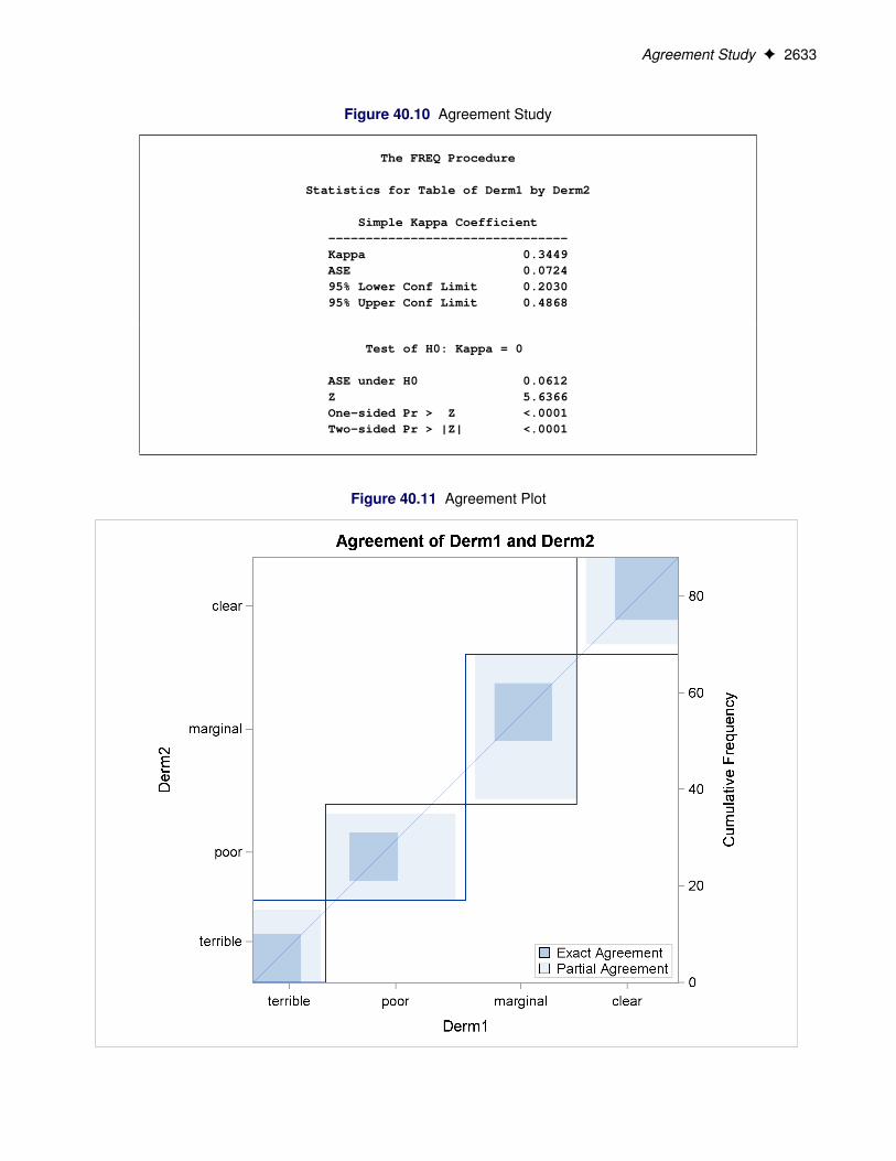
Figure 40.10 and Figure 40.11 show the results. The kappa coefficient has the value 0.3449, which indicatessome agreement between the dermatologists, and the hypothesis test confirms that you can reject the nullhypothesis of no agreement. This conclusion is further supported by the confidence interval of (0.2030,0.4868), which suggests that the true kappa is greater than zero. The AGREE option also produces Bowker’stest for symmetry and the weighted kappa coefficient, but that output is not shown here. Figure 40.11 displaysthe agreement plot for the ratings of the two dermatologists.
Agreement Study F 2633
Figure 40.10 Agreement Study
The FREQ Procedure
Statistics for Table of Derm1 by Derm2
Simple Kappa Coefficient--------------------------------Kappa 0.3449ASE 0.072495% Lower Conf Limit 0.203095% Upper Conf Limit 0.4868
Test of H0: Kappa = 0
ASE under H0 0.0612Z 5.6366One-sided Pr > Z <.0001Two-sided Pr > |Z| <.0001
Figure 40.11 Agreement Plot
2634 F Chapter 40: The FREQ Procedure
Syntax: FREQ ProcedureThe following statements are available in the FREQ procedure:
PROC FREQ < options > ;BY variables ;EXACT statistic-options < / computation-options > ;OUTPUT < OUT=SAS-data-set > output-options ;TABLES requests < / options > ;TEST options ;WEIGHT variable < / option > ;
The PROC FREQ statement is the only required statement for the FREQ procedure. If you specify thefollowing statements, PROC FREQ produces a one-way frequency table for each variable in the most recentlycreated data set.
proc freq;run;
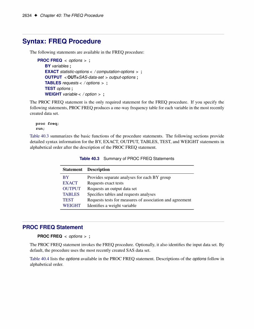
Table 40.3 summarizes the basic functions of the procedure statements. The following sections providedetailed syntax information for the BY, EXACT, OUTPUT, TABLES, TEST, and WEIGHT statements inalphabetical order after the description of the PROC FREQ statement.
Table 40.3 Summary of PROC FREQ Statements
Statement Description
BY Provides separate analyses for each BY groupEXACT Requests exact testsOUTPUT Requests an output data setTABLES Specifies tables and requests analysesTEST Requests tests for measures of association and agreementWEIGHT Identifies a weight variable
PROC FREQ StatementPROC FREQ < options > ;
The PROC FREQ statement invokes the FREQ procedure. Optionally, it also identifies the input data set. Bydefault, the procedure uses the most recently created SAS data set.
Table 40.4 lists the options available in the PROC FREQ statement. Descriptions of the options follow inalphabetical order.
PROC FREQ Statement F 2635
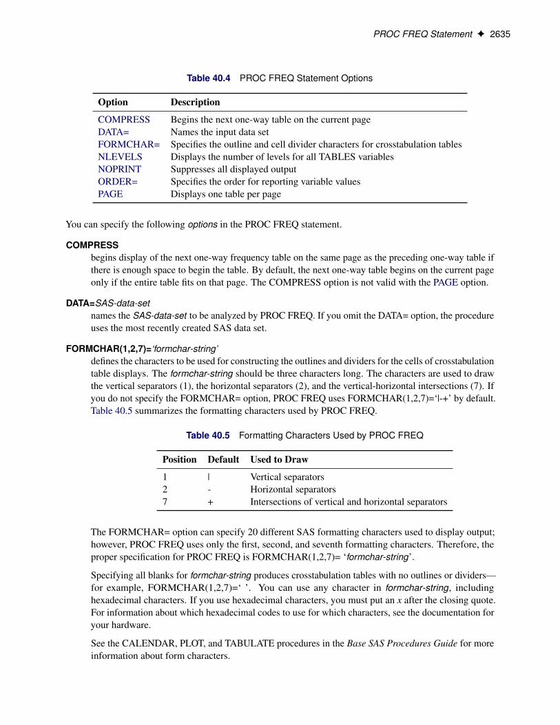
Table 40.4 PROC FREQ Statement Options
Option Description
COMPRESS Begins the next one-way table on the current pageDATA= Names the input data setFORMCHAR= Specifies the outline and cell divider characters for crosstabulation tablesNLEVELS Displays the number of levels for all TABLES variablesNOPRINT Suppresses all displayed outputORDER= Specifies the order for reporting variable valuesPAGE Displays one table per page
You can specify the following options in the PROC FREQ statement.
COMPRESSbegins display of the next one-way frequency table on the same page as the preceding one-way table ifthere is enough space to begin the table. By default, the next one-way table begins on the current pageonly if the entire table fits on that page. The COMPRESS option is not valid with the PAGE option.
DATA=SAS-data-setnames the SAS-data-set to be analyzed by PROC FREQ. If you omit the DATA= option, the procedureuses the most recently created SAS data set.
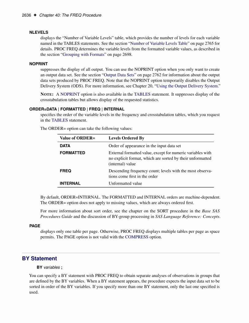
FORMCHAR(1,2,7)=‘formchar-string’defines the characters to be used for constructing the outlines and dividers for the cells of crosstabulationtable displays. The formchar-string should be three characters long. The characters are used to drawthe vertical separators (1), the horizontal separators (2), and the vertical-horizontal intersections (7). Ifyou do not specify the FORMCHAR= option, PROC FREQ uses FORMCHAR(1,2,7)=‘|-+’ by default.Table 40.5 summarizes the formatting characters used by PROC FREQ.
Table 40.5 Formatting Characters Used by PROC FREQ
Position Default Used to Draw
1 | Vertical separators2 - Horizontal separators7 + Intersections of vertical and horizontal separators
The FORMCHAR= option can specify 20 different SAS formatting characters used to display output;however, PROC FREQ uses only the first, second, and seventh formatting characters. Therefore, theproper specification for PROC FREQ is FORMCHAR(1,2,7)= ‘formchar-string’.
Specifying all blanks for formchar-string produces crosstabulation tables with no outlines or dividers—for example, FORMCHAR(1,2,7)=‘ ’. You can use any character in formchar-string, includinghexadecimal characters. If you use hexadecimal characters, you must put an x after the closing quote.For information about which hexadecimal codes to use for which characters, see the documentation foryour hardware.
See the CALENDAR, PLOT, and TABULATE procedures in the Base SAS Procedures Guide for moreinformation about form characters.
2636 F Chapter 40: The FREQ Procedure
NLEVELSdisplays the “Number of Variable Levels” table, which provides the number of levels for each variablenamed in the TABLES statements. See the section “Number of Variable Levels Table” on page 2765 fordetails. PROC FREQ determines the variable levels from the formatted variable values, as described inthe section “Grouping with Formats” on page 2698.
NOPRINTsuppresses the display of all output. You can use the NOPRINT option when you only want to createan output data set. See the section “Output Data Sets” on page 2762 for information about the outputdata sets produced by PROC FREQ. Note that the NOPRINT option temporarily disables the OutputDelivery System (ODS). For more information, see Chapter 20, “Using the Output Delivery System.”
NOTE: A NOPRINT option is also available in the TABLES statement. It suppresses display of thecrosstabulation tables but allows display of the requested statistics.
ORDER=DATA | FORMATTED | FREQ | INTERNALspecifies the order of the variable levels in the frequency and crosstabulation tables, which you requestin the TABLES statement.
The ORDER= option can take the following values:
Value of ORDER= Levels Ordered By
DATA Order of appearance in the input data set
FORMATTED External formatted value, except for numeric variables withno explicit format, which are sorted by their unformatted(internal) value
FREQ Descending frequency count; levels with the most observa-tions come first in the order
INTERNAL Unformatted value
By default, ORDER=INTERNAL. The FORMATTED and INTERNAL orders are machine-dependent.The ORDER= option does not apply to missing values, which are always ordered first.
For more information about sort order, see the chapter on the SORT procedure in the Base SASProcedures Guide and the discussion of BY-group processing in SAS Language Reference: Concepts.
PAGEdisplays only one table per page. Otherwise, PROC FREQ displays multiple tables per page as spacepermits. The PAGE option is not valid with the COMPRESS option.
BY StatementBY variables ;
You can specify a BY statement with PROC FREQ to obtain separate analyses of observations in groups thatare defined by the BY variables. When a BY statement appears, the procedure expects the input data set to besorted in order of the BY variables. If you specify more than one BY statement, only the last one specified isused.
EXACT Statement F 2637
If your input data set is not sorted in ascending order, use one of the following alternatives:
• Sort the data by using the SORT procedure with a similar BY statement.
• Specify the NOTSORTED or DESCENDING option in the BY statement for the FREQ procedure.The NOTSORTED option does not mean that the data are unsorted but rather that the data are arrangedin groups (according to values of the BY variables) and that these groups are not necessarily inalphabetical or increasing numeric order.
• Create an index on the BY variables by using the DATASETS procedure (in Base SAS software).
For more information about BY-group processing, see the discussion in SAS Language Reference: Concepts.For more information about the DATASETS procedure, see the discussion in the Base SAS Procedures Guide.
EXACT StatementEXACT statistic-options < / computation-options > ;
The EXACT statement requests exact tests and confidence limits for selected statistics. The statistic-optionsidentify which statistics to compute, and the computation-options specify options for computing exactstatistics. See the section “Exact Statistics” on page 2757 for details.
NOTE: PROC FREQ computes exact tests by using fast and efficient algorithms that are superior to directenumeration. Exact tests are appropriate when a data set is small, sparse, skewed, or heavily tied. Forsome large problems, computation of exact tests might require a considerable amount of time and memory.Consider using asymptotic tests for such problems. Alternatively, when asymptotic methods might not besufficient for such large problems, consider using Monte Carlo estimation of exact p-values. You can requestMonte Carlo estimation by specifying the MC computation-option in the EXACT statement. See the section“Computational Resources” on page 2759 for more information.
Statistic Options
The statistic-options specify which exact tests and confidence limits to compute. Table 40.6 lists the availablestatistic-options and the exact statistics that are computed. Descriptions of the statistic-options follow thetable in alphabetical order.
For one-way tables, exact p-values are available for binomial proportion tests, the chi-square goodness-of-fittest, and the likelihood ratio chi-square test. Exact (Clopper-Pearson) confidence limits are available for thebinomial proportion.
For two-way tables, exact p-values are available for the following tests: Pearson chi-square test, likelihoodratio chi-square test, Mantel-Haenszel chi-square test, Fisher’s exact test, Jonckheere-Terpstra test, andCochran-Armitage test for trend. Exact p-values are also available for tests of the following statistics: Pearsoncorrelation coefficient, Spearman correlation coefficient, Kendall’s tau-b, Stuart’s tau-c, Somers’ D.C jR/,Somers’ D.RjC/, simple kappa coefficient, and weighted kappa coefficient.
For 2 � 2 tables, PROC FREQ provides the exact McNemar’s test, exact confidence limits for the odds ratio,and Barnard’s unconditional exact test for the risk (proportion) difference. PROC FREQ also provides exactunconditional confidence limits for the risk difference and for the relative risk (ratio of proportions). Forstratified 2 � 2 tables, PROC FREQ provides Zelen’s exact test for equal odds ratios, exact confidence limitsfor the common odds ratio, and an exact test for the common odds ratio.

2638 F Chapter 40: The FREQ Procedure
Most of the statistic-option names listed in Table 40.6 are identical to the corresponding option names in theTABLES and OUTPUT statements. You can request exact computations for groups of statistics by usingstatistic-options that are identical to the TABLES statement options CHISQ, MEASURES, and AGREE. Forexample, when you specify the CHISQ statistic-option in the EXACT statement, PROC FREQ computesexact p-values for the Pearson chi-square, likelihood ratio chi-square, and Mantel-Haenszel chi-square testsfor two-way tables. You can request an exact test for an individual statistic by specifying the correspondingstatistic-option from the list in Table 40.6.
Using the EXACT Statement with the TABLES StatementYou must use a TABLES statement with the EXACT statement. If you use only one TABLES statement, youdo not need to specify the same options in both the TABLES and EXACT statements; when you specify astatistic-option in the EXACT statement, PROC FREQ automatically invokes the corresponding TABLESstatement option. However, when you use an EXACT statement with multiple TABLES statements, you mustspecify options in the TABLES statements to request statistics. PROC FREQ then provides exact tests orconfidence limits for those statistics that you also specify in the EXACT statement.
Table 40.6 EXACT Statement Statistic Options
Statistic Option Exact Statistics
AGREE McNemar’s test (for 2 � 2 tables), simple kappa test,weighted kappa test
BARNARD Barnard’s test (for 2 � 2 tables)BINOMIAL | BIN Binomial proportion tests for one-way tablesCHISQ Chi-square goodness-of-fit test for one-way tables;
Pearson chi-square, likelihood ratio chi-square, andMantel-Haenszel chi-square tests for two-way tables
COMOR Confidence limits for the common odds ratio,common odds ratio test (for h � 2 � 2 tables)
EQOR | ZELEN Zelen’s test for equal odds ratios (for h � 2 � 2 tables)FISHER Fisher’s exact testJT Jonckheere-Terpstra testKAPPA Test for the simple kappa coefficientKENTB | TAUB Test for Kendall’s tau-bLRCHI Likelihood ratio chi-square test (one-way and two-way tables)MCNEM McNemar’s test (for 2 � 2 tables)MEASURES Tests for the Pearson correlation and Spearman correlation,
confidence limits for the odds ratio (for 2 � 2 tables)MHCHI Mantel-Haenszel chi-square testOR | ODDSRATIO Confidence limits for the odds ratio (for 2 � 2 tables)PCHI Pearson chi-square test (one-way and two-way tables)PCORR Test for the Pearson correlation coefficientRELRISK Confidence limits for the relative risk (for 2 � 2 tables)RISKDIFF Confidence limits for the proportion difference (for 2� 2 tables)SCORR Test for the Spearman correlation coefficientSMDCR Test for Somers’ D.C jR/SMDRC Test for Somers’ D.RjC/STUTC | TAUC Test for Stuart’s tau-cTREND Cochran-Armitage test for trendWTKAP | WTKAPPA Test for the weighted kappa coefficient

EXACT Statement F 2639
You can specify the following statistic-options in the EXACT statement.
AGREErequests exact tests for the simple and weighted kappa coefficients and McNemar’s exact test. “Testsand Measures of Agreement” on page 2743 and “Exact Statistics” on page 2757 for details.
The AGREE option in the TABLES statement provides the simple and weighted kappa coefficients(with their standard errors and confidence limits) and the asymptotic McNemar’s test. The AGREEoption in the TEST statement provides asymptotic tests for the kappa coefficients.
Kappa coefficients can be computed for square two-way tables, where the number of rows equalsthe number of columns. For 2 � 2 tables, the weighted kappa coefficient equals the simple kappacoefficient, and PROC FREQ displays only the simple kappa coefficient. McNemar’s test is availablefor 2 � 2 tables.
BARNARDrequests Barnard’s exact unconditional test for the risk (proportion) difference for 2 � 2 tables. See thesection “Barnard’s Unconditional Exact Test” on page 2735 for details. The RISKDIFF option in theTABLES statement provides risk difference estimates, confidence limits, and asymptotic tests. See thesection “Risks and Risk Differences” on page 2725 for more information.
BINOMIAL
BINrequests exact tests for the binomial proportion (for one-way tables). See the section “Binomial Tests”on page 2721 for details. The BINOMIAL option in the TABLES statement provides confidence limitsand asymptotic tests for the binomial proportion. See the section “Binomial Proportion” on page 2719for more information.
CHISQrequests exact tests for the Pearson chi-square, likelihood ratio chi-square, and Mantel-Haenszelchi-square for two-way tables. See the section “Chi-Square Tests and Statistics” on page 2704 fordetails. The CHISQ option in the TABLES statement provides asymptotic tests for these statistics.
For one-way tables, the CHISQ option requests the exact chi-square goodness-of-fit test. See thesection “Chi-Square Test for One-Way Tables” on page 2704 for details.
COMORrequests an exact test and exact confidence limits for the common odds ratio for multiway 2 � 2 tables.See the section “Exact Confidence Limits for the Common Odds Ratio” on page 2754 for details. TheCMH option in the TABLES statement provides Mantel-Haenszel and logit estimates and asymptoticconfidence limits for the common odds ratio.
EQOR
ZELENrequests Zelen’s exact test for equal odds ratios, which is available for multiway 2 � 2 tables. See thesection “Zelen’s Exact Test for Equal Odds Ratios” on page 2754 for details. The CMH option in theTABLES statement provides the asymptotic Breslow-Day test for homogeneity of odds ratios.
2640 F Chapter 40: The FREQ Procedure
FISHERrequest Fisher’s exact test. See the sections “Fisher’s Exact Test” on page 2708 and “Exact Statistics”on page 2757 for details. For 2 � 2 tables, the CHISQ option in the TABLES statement providesFisher’s exact test. For general R � C tables, Fisher’s exact test is also known as the Freeman-Haltontest.
JTrequests the exact Jonckheere-Terpstra test. See the sections “Jonckheere-Terpstra Test” on page 2741and “Exact Statistics” on page 2757 for details. The JT option in the TABLES statement provides theasymptotic Jonckheere-Terpstra test.
KAPPArequests an exact test for the simple kappa coefficient. See the sections “Simple Kappa Coefficient”on page 2744 and “Exact Statistics” on page 2757 for details. The AGREE option in the TABLESstatement provides the simple kappa estimate, standard error, and confidence limits. The KAPPAoption in the TEST statement provides the asymptotic test for the simple kappa coefficient.
Kappa coefficients are defined only for square tables, where the number of rows equals the number ofcolumns. PROC FREQ does not compute kappa coefficients for tables that are not square.
KENTB
TAUBrequests an exact test for Kendall’s tau-b. See the sections “Kendall’s Tau-b” on page 2711 and “ExactStatistics” on page 2757 for details. The MEASURES option in the TABLES statement provides theKendall’s tau-b estimate and standard error. The KENTB option in the TEST statement provides anasymptotic test for Kendall’s tau-b.
LRCHIrequests an exact test for the likelihood ratio chi-square for two-way tables. See the sections “LikelihoodRatio Chi-Square Test” on page 2707 and “Exact Statistics” on page 2757 for details. For one-waytables, the LRCHI option requests an exact likelihood ratio goodness-of-fit test. See the section“Likelihood Ratio Chi-Square Test for One-Way Tables” on page 2706 for details.
The CHISQ option in the TABLES statement provides asymptotic likelihood ratio chi-square tests.
MCNEMrequests the exact McNemar’s test. See the sections “McNemar’s Test” on page 2743 and “ExactStatistics” on page 2757 for details. The AGREE option in the TABLES statement provides theasymptotic McNemar’s test.
MEASURESrequests exact tests for the Pearson and Spearman correlations. See the sections “Pearson CorrelationCoefficient” on page 2713, “Spearman Rank Correlation Coefficient” on page 2714, and “ExactStatistics” on page 2757 for details. The PCORR and SCORR options in the TEST statement provideasymptotic tests for the Pearson and Spearman correlations, respectively.
This option also requests exact confidence limits for the odds ratio for 2�2 tables. For more information,see the sections “Odds Ratio” on page 2737 and “Exact Confidence Limits for the Odds Ratio” onpage 2738. The MEASURES, OR(CL=), and RELRISK options in the TABLES statement provideasymptotic confidence limits for the odds ratio.

EXACT Statement F 2641
MHCHIrequests an exact test for the Mantel-Haenszel chi-square. See the sections “Mantel-Haenszel Chi-Square Test” on page 2707 and “Exact Statistics” on page 2757 for details. The CHISQ option in theTABLES statement provides the asymptotic Mantel-Haenszel chi-square test.
OR
ODDSRATIOrequests exact confidence limits for the odds ratio for 2 � 2 tables. For more information, see thesections “Odds Ratio” on page 2737 and “Exact Confidence Limits for the Odds Ratio” on page 2738.The MEASURES, OR(CL=), and RELRISK options in the TABLES statement provide asymptoticconfidence limits for the odds ratio.
You can set the confidence level by specifying the ALPHA= option in the TABLES statement. Thedefault of ALPHA=0.05 produces 95% confidence limits.
PCHIrequests an exact test for the Pearson chi-square for two-way tables. See the sections “Pearson Chi-Square Test for Two-Way Tables” on page 2705 and “Exact Statistics” on page 2757 for details. Forone-way tables, the PCHI option requests an exact chi-square goodness-of-fit test. See the section“Chi-Square Test for One-Way Tables” on page 2704 for details. The CHISQ option in the TABLESstatement provides asymptotic chi-square tests.
PCORRrequests an exact test for the Pearson correlation coefficient. See the sections “Pearson CorrelationCoefficient” on page 2713 and “Exact Statistics” on page 2757 for details. The MEASURES optionin the TABLES statement provides the Pearson correlation estimate and standard error. The PCORRoption in the TEST statement provides an asymptotic test for the Pearson correlation.
RELRISK < (options) >requests exact unconditional confidence limits for the relative risk for 2 � 2 tables. PROC FREQcomputes the confidence limits by inverting two separate one-sided exact tests (Santner and Snell1980). By default, this computation uses the unstandardized relative risk as the test statistic. If youspecify the RELRISK(METHOD=SCORE) option, the computation uses the score statistic (Chan andZhang 1999). For more information, see the section “Exact Unconditional Confidence Limits for theRelative Risk” on page 2739.
You can set the confidence level by specifying the ALPHA= option in the TABLES statement. Thedefault of ALPHA=0.05 produces 95% confidence limits.
The RELRISK and MEASURES options in the TABLES statement provide asymptotic confidencelimits for the relative risk. For more information, see the section “Relative Risks” on page 2739.
You can specify the following options:
COLUMN=1 | 2 | BOTHspecifies the table column for which to compute the relative risk. The default is COLUMN=1,which provides exact confidence limits for the column 1 relative risk. If you specifyCOLUMN=BOTH, PROC FREQ provides exact confidence limits for both column 1 and column2 relative risks.

2642 F Chapter 40: The FREQ Procedure
METHOD=SCORErequests exact unconditional confidence limits that are based on the score statistic (Chan andZhang 1999). For more information, see the section “Exact Unconditional Confidence Limits forthe Relative Risk” on page 2739. If you do not specify METHOD=SCORE, by default the exactconfidence limit computations are based on the unstandardized relative risk.
RISKDIFF < (options) >requests exact unconditional confidence limits for the risk difference for 2 � 2 tables. PROC FREQcomputes the confidence limits by inverting two separate one-sided exact tests (Santner and Snell1980). By default, this computation uses the unstandardized risk difference as the test statistic. If youspecify the RISKDIFF(METHOD=SCORE) option, the computation uses the score statistic (Chan andZhang 1999). See the section “Exact Unconditional Confidence Limits for the Risk Difference” onpage 2734 for more information.
You can set the confidence level by specifying the ALPHA= option in the TABLES statement. Thedefault of ALPHA=0.05 produces 95% confidence limits.
The RISKDIFF option in the TABLES statement provides asymptotic confidence limits for the riskdifference, including Wald, Newcombe, and Miettinen-Nurminen (score) confidence limits. See thesection “Risk Difference Confidence Limits” on page 2727 for more information.
You can specify the following options:
COLUMN=1 | 2 | BOTHspecifies the table column for which to compute the risk difference. The default isCOLUMN=BOTH, which provides exact confidence limits for both column 1 and column2 risk differences.
METHOD=SCORErequests exact unconditional confidence limits that are based on the score statistic (Chan andZhang 1999). See the section “Exact Unconditional Confidence Limits for the Risk Difference”on page 2734 for more information. If you do not specify METHOD=SCORE, by default theexact confidence limit computations are based on the unstandardized risk difference.
SCORRrequests an exact test for the Spearman correlation coefficient. See the sections “Spearman RankCorrelation Coefficient” on page 2714 and “Exact Statistics” on page 2757 for details. The MEASURESoption in the TABLES statement provides the Spearman correlation estimate and standard error. TheSCORR option in the TEST statement provides an asymptotic test for the Spearman correlation.
SMDCRrequests an exact test for Somers’ D.C jR/. See the sections “Somers’ D” on page 2712 and “ExactStatistics” on page 2757 for details. The MEASURES option in the TABLES statement providesSomers’ D.C jR/ estimate and the standard error. The SMDCR option in the TEST statement providesan asymptotic test for Somers’ D.C jR/.
SMDRCrequests an exact test for Somers’ D.RjC/. See the sections “Somers’ D” on page 2712 and “ExactStatistics” on page 2757 for details. The MEASURES option in the TABLES statement providesSomers’ D.RjC/ estimate and the standard error. The SMDRC option in the TEST statement requestsan asymptotic test for Somers’ D.C jR/.
EXACT Statement F 2643
STUTC
TAUCrequests an exact test for Stuart’s tau-c. See the sections “Stuart’s Tau-c” on page 2712 and “ExactStatistics” on page 2757 for details. The MEASURES option in the TABLES statement providesStuart’s tau-c estimate and the standard error. The STUTC option in the TEST statement provides anasymptotic test for Stuart’s tau-c.
TRENDrequests the exact Cochran-Armitage test for trend. See the sections “Cochran-Armitage Test for Trend”on page 2740 and “Exact Statistics” on page 2757 for details. The TREND option in the TABLESstatement provides the asymptotic Cochran-Armitage trend test. The trend test is available for tables ofdimensions 2 � C or R � 2.
WTKAP
WTKAPPArequests an exact test for the weighted kappa coefficient. See the sections “Weighted Kappa Coefficient”on page 2745 and “Exact Statistics” on page 2757 for details. The AGREE option in the TABLESstatement provides the weighted kappa estimate, standard error, and confidence limits. The WTKAPoption in the TEST statement provides the asymptotic test for the weighted kappa coefficient.
Kappa coefficients are defined only for square tables, where the number of rows equals the number ofcolumns. PROC FREQ does not compute kappa coefficients for tables that are not square. For 2 � 2tables, the weighted kappa coefficient equals the simple kappa coefficient, and PROC FREQ does notpresent separate results for the weighted kappa coefficient.
Computation Options
The computation-options specify options for computing exact statistics. You can specify the followingcomputation-options in the EXACT statement after a slash (/).
ALPHA=˛specifies the level of the confidence limits for Monte Carlo p-value estimates. The value of ˛ must bebetween 0 and 1, and the default is 0.01. A confidence level of ˛ produces 100.1 � ˛/% confidencelimits. The default of ALPHA=.01 produces 99% confidence limits for the Monte Carlo estimates.
The ALPHA= option invokes the MC option.
MAXTIME=valuespecifies the maximum clock time (in seconds) that PROC FREQ can use to compute an exactp-value. If the procedure does not complete the computation within the specified time, the computationterminates. The MAXTIME= value must be a positive number. This option is available for Monte Carloestimation of exact p-values as well as for direct exact p-value computation. For more information, seethe section “Computational Resources” on page 2759.
MCrequests Monte Carlo estimation of exact p-values instead of direct exact p-value computation. MonteCarlo estimation can be useful for large problems that require a considerable amount of time andmemory for exact computations but for which asymptotic approximations might not be sufficient. Formore information, see the section “Monte Carlo Estimation” on page 2760.

2644 F Chapter 40: The FREQ Procedure
This option is available for all EXACT statistic-options except the BINOMIAL option and the followingoptions that apply only to 2 � 2 or h � 2 � 2 tables: BARNARD, COMOR, EQOR, MCNEM, OR,RELRISK, and RISKDIFF. PROC FREQ always computes exact tests or confidence limits (not MonteCarlo estimates) for these statistics.
The ALPHA=, N=, and SEED= options invoke the MC option.
MIDPrequests exact mid p-values for the exact tests. The exact mid p-value is defined as the exact p-valueminus half the exact point probability. For more information, see the section “Definition of p-Values”on page 2758.
The MIDP option is available for all EXACT statement statistic-options except the following:BARNARD, EQOR, OR, RELRISK, and RISKDIFF. You cannot specify both the MIDP optionand the MC option.
N=nspecifies the number of samples for Monte Carlo estimation. The value of n must be a positive integer,and the default is 10,000. Larger values of n produce more precise estimates of exact p-values. Becauselarger values of n generate more samples, the computation time increases.
The N= option invokes the MC option.
PFORMAT=format-name | EXACTspecifies the display format for exact p-values. PROC FREQ applies this format to one- and two-sidedexact p-values, exact point probabilities, and exact mid p-values. By default, PROC FREQ displaysexact p-values in the PVALUE6.4 format.
You can provide a format-name or you can specify PFORMAT=EXACT to control the format of exactp-values. The value of format-name can be any standard SAS numeric format or a user-defined format.The format length must not exceed 24. For information about formats, see the FORMAT procedurein the Base SAS Procedures Guide and the FORMAT statement and SAS format in SAS Formats andInformats: Reference.
If you specify PFORMAT=EXACT, PROC FREQ uses the 6.4 format to display exact p-values that aregreater than or equal to 0.001; the procedure uses the E10.3 format to display values that are between0.000 and 0.001. This is the format that PROC FREQ uses to display exact p-values in releases beforeSAS/STAT 12.3. Beginning in SAS/STAT 12.3, by default PROC FREQ uses the PVALUE6.4 formatto display exact p-values.
POINTrequests exact point probabilities for the exact tests. The exact point probability is the exact probabilitythat the test statistic equals the observed value. For more information, see the section “Definition ofp-Values” on page 2758.
The POINT option is available for all EXACT statement statistic-options except the following:BARNARD, EQOR, OR, RELRISK, and RISKDIFF. You cannot specify both the POINT option andthe MC option.
SEED=numberspecifies the initial seed for random number generation for Monte Carlo estimation. The value of theSEED= option must be an integer. If you do not specify the SEED= option or if the SEED= value isnegative or zero, PROC FREQ uses the time of day from the computer’s clock to obtain the initial seed.
The SEED= option invokes the MC option.

OUTPUT Statement F 2645
OUTPUT StatementOUTPUT < OUT=SAS-data-set > output-options ;
The OUTPUT statement creates a SAS data set that contains statistics that are computed by PROC FREQ.Table 40.7 lists the statistics that can be stored in the output data set. You identify which statistics to includeby specifying output-options.
You must use a TABLES statement with the OUTPUT statement. The OUTPUT statement stores statistics foronly one table request. If you use multiple TABLES statements, the contents of the output data set correspondto the last TABLES statement. If you use multiple table requests in a single TABLES statement, the contentsof the output data set correspond to the last table request. Only one OUTPUT statement is allowed in a singleinvocation of the procedure.
For a one-way or two-way table, the output data set contains one observation that stores the requestedstatistics for the table. For a multiway table, the output data set contains an observation for each two-waytable (stratum) of the multiway crosstabulation. If you request summary statistics for the multiway table, theoutput data set also contains an observation that stores the across-strata summary statistics. If you use a BYstatement, the output data set contains an observation or set of observations for each BY group. For moreinformation about the contents of the output data set, see the section “Contents of the OUTPUT StatementOutput Data Set” on page 2763.
The output data set that is created by the OUTPUT statement is not the same as the output data set thatis created by the OUT= option in the TABLES statement. The OUTPUT statement creates a data set thatcontains statistics (such as the Pearson chi-square and its p-value), and the OUT= option in the TABLESstatement creates a data set that contains frequency table counts and percentages. See the section “OutputData Sets” on page 2762 for more information.
As an alternative to the OUTPUT statement, you can use the Output Delivery System (ODS) to store statisticsthat PROC FREQ computes. ODS can create a SAS data set from any table that PROC FREQ produces. Seethe section “ODS Table Names” on page 2773 for more information.
You can specify the following options in the OUTPUT statement:
OUT=SAS-data-setspecifies the name of the output data set. When you use an OUTPUT statement but do not use theOUT= option, PROC FREQ creates a data set and names it by using the DATAn convention.
output-optionsspecify the statistics to include in the output data set. Table 40.7 lists the output-options that areavailable in the OUTPUT statement, together with the TABLES statement options that are required toproduce the statistics. Descriptions of the output-options follow the table in alphabetical order.
You can specify output-options to request individual statistics, or you can request groups of statisticsby using output-options that are identical to the group options in the TABLES statement (for example,the CHISQ, MEASURES, CMH, AGREE, and ALL options).
When you specify an output-option, the output data set includes statistics from the correspondinganalysis. In addition to the estimate or test statistic, the output data set includes associated values suchas standard errors, confidence limits, p-values, and degrees of freedom. See the section “Contents ofthe OUTPUT Statement Output Data Set” on page 2763 for details.

2646 F Chapter 40: The FREQ Procedure
To store a statistic in the output data set, you must also request computation of that statistic withthe appropriate TABLES, EXACT, or TEST statement option. For example, the PCHI output-optionincludes the Pearson chi-square in the output data set. You must also request computation of thePearson chi-square by specifying the CHISQ option in the TABLES statement. Or, if you use only oneTABLES statement, you can request computation of the Pearson chi-square by specifying the PCHIor CHISQ option in the EXACT statement. Table 40.7 lists the TABLES statement options that arerequired to produce the OUTPUT data set statistics.
Table 40.7 OUTPUT Statement Output Options
Output Option Output Data Set Statistics Required TABLESStatement Option
AGREE McNemar’s test (2 � 2 tables), Bowker’s test, AGREEsimple and weighted kappas; for multiple strata,overall simple and weighted kappas, tests for equalkappas, and Cochran’s Q (h � 2 � 2 tables)
AJCHI Continuity-adjusted chi-square (2 � 2 tables) CHISQALL CHISQ, MEASURES, and CMH statistics; ALL
N (number of nonmissing observations)BDCHI Breslow-Day test (h � 2 � 2 tables) CMH, CMH1, or CMH2BINOMIAL | BIN Binomial statistics (one-way tables) BINOMIALCHISQ For one-way tables, goodness-of-fit test; CHISQ
for two-way tables, Pearson, likelihood ratio,continuity-adjusted, and Mantel-Haenszelchi-squares, Fisher’s exact test (2 � 2 tables),phi and contingency coefficients, Cramér’s V
CMH Cochran-Mantel-Haenszel (CMH) correlation, CMHrow mean scores (ANOVA), and generalassociation statistics; for 2 � 2 tables, logitand Mantel-Haenszel common odds ratiosand relative risks, Breslow-Day test
CMH1 CMH statistics, except row mean scores (ANOVA) CMH or CMH1and general association statistics
CMH2 CMH statistics, except general association statistic CMH or CMH2CMHCOR CMH correlation statistic CMH, CMH1, or CMH2CMHGA CMH general association statistic CMHCMHRMS CMH row mean scores (ANOVA) statistic CMH or CMH2COCHQ Cochran’s Q (h � 2 � 2 tables) AGREECONTGY Contingency coefficient CHISQCRAMV Cramér’s V CHISQEQKAP Test for equal simple kappas AGREEEQOR | ZELEN Zelen’s test for equal odds ratios (h � 2 � 2 tables) CMH and EXACT EQOREQWKP Test for equal weighted kappas AGREEFISHER Fisher’s exact test CHISQ or FISHER 1
GAMMA Gamma MEASURESGS | GAILSIMON Gail-Simon test CMH(GAILSIMON)
1CHISQ computes Fisher’s exact test for 2 � 2 tables. Use the FISHER option to compute Fisher’s exact test for general r � ctables.

OUTPUT Statement F 2647
Table 40.7 continued
Output Option Output Data Set Statistics Required TABLESStatement Option
JT Jonckheere-Terpstra test JTKAPPA Simple kappa coefficient AGREEKENTB | TAUB Kendall’s tau-b MEASURESLAMCR Lambda asymmetric .C jR/ MEASURESLAMDAS Lambda symmetric MEASURESLAMRC Lambda asymmetric .RjC/ MEASURESLGOR Logit common odds ratio CMH, CMH1, or CMH2LGRRC1 Logit common relative risk, column 1 CMH, CMH1, or CMH2LGRRC2 Logit common relative risk, column 2 CMH, CMH1, or CMH2LRCHI Likelihood ratio chi-square CHISQMCNEM McNemar’s test (2 � 2 tables) AGREEMEASURES Gamma, Kendall’s tau-b, Stuart’s tau-c, MEASURES
Somers’ D.C jR/ and D.RjC/, Pearson andSpearman correlations, lambda asymmetric.C jR/ and .RjC/, lambda symmetric,uncertainty coefficients .C jR/ and .RjC/,symmetric uncertainty coefficient;odds ratio and relative risks (2 � 2 tables)
MHCHI Mantel-Haenszel chi-square CHISQMHOR | COMOR Mantel-Haenszel common odds ratio CMH, CMH1, or CMH2MHRRC1 Mantel-Haenszel common relative risk, column 1 CMH, CMH1, or CMH2MHRRC2 Mantel-Haenszel common relative risk, column 2 CMH, CMH1, or CMH2N Number of nonmissing observationsNMISS Number of missing observationsOR | ODDSRATIO Odds ratio (2 � 2 tables) MEASURES or RELRISKPCHI Chi-square goodness-of-fit test (one-way tables), CHISQ
Pearson chi-square (two-way tables)PCORR Pearson correlation coefficient MEASURESPHI Phi coefficient CHISQPLCORR Polychoric correlation coefficient PLCORRRDIF1 Column 1 risk difference (row 1 – row 2) RISKDIFFRDIF2 Column 2 risk difference (row 1 – row 2) RISKDIFFRELRISK Odds ratio and relative risks (2 � 2 tables) MEASURES or RELRISKRISKDIFF Risks and risk differences (2 � 2 tables) RISKDIFFRISKDIFF1 Risks and risk difference, column 1 RISKDIFFRISKDIFF2 Risks and risk difference, column 2 RISKDIFFRRC1 | RELRISK1 Relative risk, column 1 MEASURES or RELRISKRRC2 | RELRISK2 Relative risk, column 2 MEASURES or RELRISKRSK1 | RISK1 Column 1 overall risk RISKDIFFRSK11 | RISK11 Column 1 risk for row 1 RISKDIFFRSK12 | RISK12 Column 2 risk for row 1 RISKDIFFRSK2 | RISK2 Column 2 overall risk RISKDIFFRSK21 | RISK21 Column 1 risk for row 2 RISKDIFFRSK22 | RISK22 Column 2 risk for row 2 RISKDIFF

2648 F Chapter 40: The FREQ Procedure
Table 40.7 continued
Output Option Output Data Set Statistics Required TABLESStatement Option
SCORR Spearman correlation coefficient MEASURESSMDCR Somers’ D.C jR/ MEASURESSMDRC Somers’ D.RjC/ MEASURESSTUTC | TAUC Stuart’s tau-c MEASURESTREND Cochran-Armitage test for trend TRENDTSYMM | BOWKER Bowker’s test of symmetry AGREEU Symmetric uncertainty coefficient MEASURESUCR Uncertainty coefficient .C jR/ MEASURESURC Uncertainty coefficient .RjC/ MEASURESWTKAP | WTKAPPA Weighted kappa coefficient AGREE
You can specify the following output-options in the OUTPUT statement.
AGREEincludes the following tests and measures of agreement in the output data set: McNemar’s test (for 2�2tables), Bowker’s test of symmetry, the simple kappa coefficient, and the weighted kappa coefficient.For multiway tables, the AGREE option also includes the following statistics in the output data set:overall simple and weighted kappa coefficients, tests for equal simple and weighted kappa coefficients,and Cochran’s Q test.
The AGREE option in the TABLES statement requests computation of tests and measures of agreement.See the section “Tests and Measures of Agreement” on page 2743 for details about these statistics.
AGREE statistics are computed only for square tables, where the number of rows equals the numberof columns. PROC FREQ provides Bowker’s test of symmetry and weighted kappa coefficients onlyfor tables larger than 2 � 2. (For 2 � 2 tables, Bowker’s test is identical to McNemar’s test, and theweighted kappa coefficient equals the simple kappa coefficient.) Cochran’s Q is available for multiway2 � 2 tables.
AJCHIincludes the continuity-adjusted chi-square in the output data set. The continuity-adjusted chi-squareis available for 2 � 2 tables and is provided by the CHISQ option in the TABLES statement. See thesection “Continuity-Adjusted Chi-Square Test” on page 2707 for details.
ALLincludes all statistics that are requested by the CHISQ, MEASURES, and CMH output-options in theoutput data set. ALL also includes the number of nonmissing observations, which you can requestindividually by specifying the N output-option.
BDCHIincludes the Breslow-Day test in the output data set. The Breslow-Day test for homogeneity of oddsratios is computed for multiway 2 � 2 tables and is provided by the CMH, CMH1, and CMH2 optionsin the TABLES statement. See the section “Breslow-Day Test for Homogeneity of the Odds Ratios”on page 2753 for details.

OUTPUT Statement F 2649
BINOMIAL
BINincludes the binomial proportion estimate, confidence limits, and tests in the output data set. TheBINOMIAL option in the TABLES statement requests computation of binomial statistics, which areavailable for one-way tables. See the section “Binomial Proportion” on page 2719 for details.
CHISQincludes the following chi-square tests and measures in the output data set for two-way tables: Pearsonchi-square, likelihood ratio chi-square, Mantel-Haenszel chi-square, phi coefficient, contingencycoefficient, and Cramér’s V. For 2�2 tables, CHISQ also includes Fisher’s exact test and the continuity-adjusted chi-square in the output data set. See the section “Chi-Square Tests and Statistics” onpage 2704 for details. For one-way tables, CHISQ includes the chi-square goodness-of-fit test in theoutput data set. See the section “Chi-Square Test for One-Way Tables” on page 2704 for details. TheCHISQ option in the TABLES statement requests computation of these statistics.
If you specify the CHISQ(WARN=OUTPUT) option in the TABLES statement, the CHISQ option alsoincludes the variable WARN_PCHI in the output data set. This variable indicates the validity warningfor the asymptotic Pearson chi-square test.
CMHincludes the following Cochran-Mantel-Haenszel statistics in the output data set: correlation, rowmean scores (ANOVA), and general association. For 2 � 2 tables, the CMH option also includesthe Mantel-Haenszel and logit estimates of the common odds ratio and relative risks. For multiway(stratified) 2 � 2 tables, the CMH option includes the Breslow-Day test for homogeneity of odds ratios.The CMH option in the TABLES statement requests computation of these statistics. See the section“Cochran-Mantel-Haenszel Statistics” on page 2748 for details.
If you specify the CMH(MF) option in the TABLES statement, the CMH option includes the Mantel-Fleiss analysis in the output data set. The variables MF_CMH and WARN_CMH contain the Mantel-Fleiss criterion and the warning indicator, respectively.
CMH1includes the CMH statistics in the output data set, with the exception of the row mean scores (ANOVA)statistic and the general association statistic. The CMH1 option in the TABLES statement requestscomputation of these statistics. See the section “Cochran-Mantel-Haenszel Statistics” on page 2748for details.
CMH2includes the CMH statistics in the output data set, with the exception of the general association statistic.The CMH2 option in the TABLES statement requests computation of these statistics. See the section“Cochran-Mantel-Haenszel Statistics” on page 2748 for details.
CMHCORincludes the Cochran-Mantel-Haenszel correlation statistic in the output data set. The CMH option inthe TABLES statement requests computation of this statistic. See the section “Correlation Statistic” onpage 2749 for details.
CMHGAincludes the Cochran-Mantel-Haenszel general association statistic in the output data set. The CMHoption in the TABLES statement requests computation of this statistic. See the section “GeneralAssociation Statistic” on page 2750 for details.

2650 F Chapter 40: The FREQ Procedure
CMHRMSincludes the Cochran-Mantel-Haenszel row mean scores (ANOVA) statistic in the output data set. TheCMH option in the TABLES statement requests computation of this statistic. See the section “ANOVA(Row Mean Scores) Statistic” on page 2750 for details.
COCHQincludes Cochran’s Q test in the output data set. The AGREE option in the TABLES statement requestscomputation of this test, which is available for multiway 2 � 2 tables. See the section “Cochran’s QTest” on page 2747 for details.
CONTGYincludes the contingency coefficient in the output data set. The CHISQ option in the TABLES statementrequests computation of the contingency coefficient. See the section “Contingency Coefficient” onpage 2709 for details.
CRAMVincludes Cramér’s V in the output data set. The CHISQ option in the TABLES statement requestscomputation of Cramér’s V. See the section “Cramér’s V” on page 2709 for details.
EQKAPincludes the test for equal simple kappa coefficients in the output data set. The AGREE option in theTABLES statement requests computation of this test, which is available for multiway, square (h� r � r)tables. See the section “Tests for Equal Kappa Coefficients” on page 2747 for details.
EQOR
ZELENincludes Zelen’s exact test for equal odds ratios in the output data set. The EQOR option in the EXACTstatement requests computation of this test, which is available for multiway 2 � 2 tables. See thesection “Zelen’s Exact Test for Equal Odds Ratios” on page 2754 for details.
EQWKPincludes the test for equal weighted kappa coefficients in the output data set. The AGREE optionin the TABLES statement requests computation of this test. The test for equal weighted kappas isavailable for multiway, square (h � r � r) tables where r > 2. See the section “Tests for Equal KappaCoefficients” on page 2747 for details.
FISHERincludes Fisher’s exact test in the output data set. For 2 � 2 tables, the CHISQ option in the TABLESstatement provides Fisher’s exact test. For tables larger than 2 � 2, the FISHER option in the EXACTstatement provides Fisher’s exact test. See the section “Fisher’s Exact Test” on page 2708 for details.
GAMMAincludes the gamma statistic in the output data set. The MEASURES option in the TABLES statementrequests computation of the gamma statistic. See the section “Gamma” on page 2711 for details.
GS
GAILSIMONincludes the Gail-Simon test for qualitative interaction in the output data set. The CMH(GAILSIMON)option in the TABLES statement requests computation of this test. See the section “Gail-Simon Testfor Qualitative Interactions” on page 2756 for details.
OUTPUT Statement F 2651
JTincludes the Jonckheere-Terpstra test in the output data set. The JT option in the TABLES statementrequests the Jonckheere-Terpstra test. See the section “Jonckheere-Terpstra Test” on page 2741 fordetails.
KAPPAincludes the simple kappa coefficient in the output data set. The AGREE option in the TABLESstatement requests computation of kappa, which is available for square tables (where the number ofrows equals the number of columns). For multiway square tables, the KAPPA option also includesthe overall kappa coefficient in the output data set. See the sections “Simple Kappa Coefficient” onpage 2744 and “Overall Kappa Coefficient” on page 2747 for details.
KENTB
TAUBincludes Kendall’s tau-b in the output data set. The MEASURES option in the TABLES statementrequests computation of Kendall’s tau-b. See the section “Kendall’s Tau-b” on page 2711 for details.
LAMCRincludes the asymmetric lambda �.C jR/ in the output data set. The MEASURES option in theTABLES statement requests computation of lambda. See the section “Lambda (Asymmetric)” onpage 2716 for details.
LAMDASincludes the symmetric lambda in the output data set. The MEASURES option in the TABLESstatement requests computation of lambda. See the section “Lambda (Symmetric)” on page 2717 fordetails.
LAMRCincludes the asymmetric lambda �.RjC/ in the output data set. The MEASURES option in theTABLES statement requests computation of lambda. See the section “Lambda (Asymmetric)” onpage 2716 for details.
LGORincludes the logit estimate of the common odds ratio in the output data set. The CMH option in theTABLES statement requests computation of this statistic, which is available for 2 � 2 tables. See thesection “Adjusted Odds Ratio and Relative Risk Estimates” on page 2751 for details.
LGRRC1includes the logit estimate of the common relative risk (column 1) in the output data set. The CMHoption in the TABLES statement requests computation of this statistic, which is available for 2 � 2tables. See the section “Adjusted Odds Ratio and Relative Risk Estimates” on page 2751 for details.
LGRRC2includes the logit estimate of the common relative risk (column 2) in the output data set. The CMHoption in the TABLES statement requests computation of this statistic, which is available for 2 � 2tables. See the section “Adjusted Odds Ratio and Relative Risk Estimates” on page 2751 for details.
LRCHIincludes the likelihood ratio chi-square in the output data set. The CHISQ option in the TABLESstatement requests computation of the likelihood ratio chi-square. See the section “Likelihood RatioChi-Square Test” on page 2707 for details.

2652 F Chapter 40: The FREQ Procedure
MCNEMincludes McNemar’s test (for 2 � 2 tables) in the output data set. The AGREE option in the TABLESstatement requests computation of McNemar’s test. See the section “McNemar’s Test” on page 2743for details.
MEASURESincludes the following measures of association in the output data set: gamma, Kendall’s tau-b, Stuart’stau-c, Somers’ D.C jR/, Somers’ D.RjC/, Pearson and Spearman correlation coefficients, lambda(symmetric and asymmetric), and uncertainty coefficients (symmetric and asymmetric). For 2�2 tables,the MEASURES option also includes the odds ratio, column 1 relative risk, and column 2 relative risk.The MEASURES option in the TABLES statement requests computation of these statistics. See thesection “Measures of Association” on page 2709 for details.
MHCHIincludes the Mantel-Haenszel chi-square in the output data set. The CHISQ option in the TABLESstatement requests computation of the Mantel-Haenszel chi-square. See the section “Mantel-HaenszelChi-Square Test” on page 2707 for details.
MHOR
COMORincludes the Mantel-Haenszel estimate of the common odds ratio in the output data set. The CMHoption in the TABLES statement requests computation of this statistic, which is available for 2 � 2tables. See the section “Adjusted Odds Ratio and Relative Risk Estimates” on page 2751 for details.
MHRRC1includes the Mantel-Haenszel estimate of the common relative risk (column 1) in the output data set.The CMH option in the TABLES statement requests computation of this statistic, which is availablefor 2 � 2 tables. See the section “Adjusted Odds Ratio and Relative Risk Estimates” on page 2751 fordetails.
MHRRC2includes the Mantel-Haenszel estimate of the common relative risk (column 2) in the output data set.The CMH option in the TABLES statement requests computation of this statistic, which is availablefor 2 � 2 tables. See the section “Adjusted Odds Ratio and Relative Risk Estimates” on page 2751 fordetails.
Nincludes the number of nonmissing observations in the output data set.
NMISSincludes the number of missing observations in the output data set. See the section “Missing Values”on page 2699 for details about how PROC FREQ handles missing values.
OR
ODDSRATIO
RRORincludes the odds ratio (for 2 � 2 tables) in the output data set. The MEASURES, OR(CL=), andRELRISK options in the TABLES statement request this statistic. For more information, see thesection “Odds Ratio” on page 2737.

OUTPUT Statement F 2653
PCHIincludes the Pearson chi-square in the output data set for two-way tables. See the section “PearsonChi-Square Test for Two-Way Tables” on page 2705 for details. For one-way tables, the PCHI optionincludes the chi-square goodness-of-fit test in the output data set. See the section “Chi-Square Test forOne-Way Tables” on page 2704 for details. The CHISQ option in the TABLES statement requestscomputation of these statistics.
If you specify the CHISQ(WARN=OUTPUT) option in the TABLES statement, the PCHI option alsoincludes the variable WARN_PCHI in the output data set. This variable indicates the validity warningfor the asymptotic Pearson chi-square test.
PCORRincludes the Pearson correlation coefficient in the output data set. The MEASURES option in the TA-BLES statement requests computation of the Pearson correlation. See the section “Pearson CorrelationCoefficient” on page 2713 for details.
PHIincludes the phi coefficient in the output data set. The CHISQ option in the TABLES statement requestscomputation of the phi coefficient. See the section “Phi Coefficient” on page 2709 for details.
PLCORRincludes the polychoric correlation coefficient in the output data set. For 2 � 2 tables, this statisticis known as the tetrachoric correlation coefficient. The PLCORR option in the TABLES statementrequests computation of the polychoric correlation. See the section “Polychoric Correlation” onpage 2715 for details.
RDIF1includes the column 1 risk difference (row 1 – row 2) in the output data set. The RISKDIFF optionin the TABLES statement requests computation of risks and risk differences, which are available for2 � 2 tables. See the section “Risks and Risk Differences” on page 2725 for details.
RDIF2includes the column 2 risk difference (row 1 – row 2) in the output data set. The RISKDIFF optionin the TABLES statement requests computation of risks and risk differences, which are available for2 � 2 tables. See the section “Risks and Risk Differences” on page 2725 for details.
RELRISKincludes the column 1 and column 2 relative risks (for 2 � 2 tables) in the output data set. TheMEASURES and RELRISK options in the TABLES statement request these statistics. For moreinformation, see the section “Relative Risks” on page 2739.
RISKDIFFincludes risks (binomial proportions) and risk differences for 2 � 2 tables in the output data set. Thesestatistics include the row 1 risk, row 2 risk, total (overall) risk, and risk difference (row 1 – row 2) forcolumn 1 and column 2. The RISKDIFF option in the TABLES statement requests computation ofthese statistics. See the section “Risks and Risk Differences” on page 2725 for details.
RISKDIFF1includes column 1 risks (binomial proportions) and risk differences for 2 � 2 tables in the output dataset. These statistics include the row 1 risk, row 2 risk, total (overall) risk, and risk difference (row 1 –row 2). The RISKDIFF option in the TABLES statement requests computation of these statistics. Seethe section “Risks and Risk Differences” on page 2725 for details.
2654 F Chapter 40: The FREQ Procedure
RISKDIFF2includes column 2 risks (binomial proportions) and risk differences for 2 � 2 tables in the output dataset. These statistics include the row 1 risk, row 2 risk, total (overall) risk, and risk difference (row 1 –row 2). The RISKDIFF option in the TABLES statement requests computation of these statistics. Seethe section “Risks and Risk Differences” on page 2725 for details.
RRC1
RELRISK1includes the column 1 relative risk in the output data set. The MEASURES and RELRISK optionsin the TABLES statement request relative risks, which are available for 2 � 2 tables. See the section“Odds Ratio and Relative Risks for 2 x 2 Tables” on page 2737 for details.
RRC2
RELRISK2includes the column 2 relative risk in the output data set. The MEASURES and RELRISK optionsin the TABLES statement request relative risks, which are available for 2 � 2 tables. See the section“Odds Ratio and Relative Risks for 2 x 2 Tables” on page 2737 for details.
RSK1
RISK1includes the overall column 1 risk in the output data set. The RISKDIFF option in the TABLESstatement requests computation of risks and risk differences, which are available for 2 � 2 tables. Seethe section “Risks and Risk Differences” on page 2725 for details.
RSK11
RISK11includes the column 1 risk for row 1 in the output data set. The RISKDIFF option in the TABLESstatement requests computation of risks and risk differences, which are available for 2 � 2 tables. Seethe section “Risks and Risk Differences” on page 2725 for details.
RSK12
RISK12includes the column 2 risk for row 1 in the output data set. The RISKDIFF option in the TABLESstatement requests computation of risks and risk differences, which are available for 2 � 2 tables. Seethe section “Risks and Risk Differences” on page 2725 for details.
RSK2
RISK2includes the overall column 2 risk in the output data set. The RISKDIFF option in the TABLES state-ment requests computation of risks and risk differences. See the section “Risks and Risk Differences”on page 2725 for details.
RSK21
RISK21includes the column 1 risk for row 2 in the output data set. The RISKDIFF option in the TABLESstatement requests computation of risks and risk differences, which are available for 2 � 2 tables. Seethe section “Risks and Risk Differences” on page 2725 for details.

OUTPUT Statement F 2655
RSK22
RISK22includes the column 2 risk for row 2 in the output data set. The RISKDIFF option in the TABLESstatement requests computation of risks and risk differences, which are available for 2 � 2 tables. Seethe section “Risks and Risk Differences” on page 2725 for details.
SCORRincludes the Spearman correlation coefficient in the output data set. The MEASURES option in theTABLES statement requests computation of the Spearman correlation. See the section “SpearmanRank Correlation Coefficient” on page 2714 for details.
SMDCRincludes Somers’ D.C jR/ in the output data set. The MEASURES option in the TABLES statementrequests computation of Somers’ D. See the section “Somers’ D” on page 2712 for details.
SMDRCincludes Somers’ D.RjC/ in the output data set. The MEASURES option in the TABLES statementrequests computation of Somers’ D. See the section “Somers’ D” on page 2712 for details.
STUTC
TAUCincludes Stuart’s tau-c in the output data set. The MEASURES option in the TABLES statementrequests computation of tau-c. See the section “Stuart’s Tau-c” on page 2712 for details.
TRENDincludes the Cochran-Armitage test for trend in the output data set. The TREND option in the TABLESstatement requests computation of the trend test. This test is available for tables of dimension 2 � C orR � 2. See the section “Cochran-Armitage Test for Trend” on page 2740 for details.
TSYMM
BOWKERincludes Bowker’s test of symmetry in the output data set. The AGREE option in the TABLESstatement requests computation of Bowker’s test. See the section “Bowker’s Test of Symmetry” onpage 2744 for details.
Uincludes the uncertainty coefficient (symmetric) in the output data set. The MEASURES option in theTABLES statement requests computation of the uncertainty coefficient. See the section “UncertaintyCoefficient (Symmetric)” on page 2718 for details.
UCRincludes the asymmetric uncertainty coefficient U.C jR/ in the output data set. The MEASURESoption in the TABLES statement requests computation of the uncertainty coefficient. See the section“Uncertainty Coefficients (Asymmetric)” on page 2718 for details.
URCincludes the asymmetric uncertainty coefficient U.RjC/ in the output data set. The MEASURESoption in the TABLES statement requests computation of the uncertainty coefficient. See the section“Uncertainty Coefficients (Asymmetric)” on page 2718 for details.
2656 F Chapter 40: The FREQ Procedure
WTKAP
WTKAPPAincludes the weighted kappa coefficient in the output data set. The AGREE option in the TABLESstatement requests computation of weighted kappa, which is available for square tables larger than2 � 2. For multiway tables, the WTKAP option also includes the overall weighted kappa coefficient inthe output data set. See the sections “Weighted Kappa Coefficient” on page 2745 and “Overall KappaCoefficient” on page 2747 for details.
TABLES StatementTABLES requests < / options > ;
The TABLES statement requests one-way to n-way frequency and crosstabulation tables and statistics forthose tables.
If you omit the TABLES statement, PROC FREQ generates one-way frequency tables for all data set variablesthat are not listed in the other statements.
The following argument is required in the TABLES statement.
requestsspecify the frequency and crosstabulation tables to produce. A request is composed of one variablename or several variable names separated by asterisks. To request a one-way frequency table, use asingle variable. To request a two-way crosstabulation table, use an asterisk between two variables. Torequest a multiway table (an n-way table, where n>2), separate the desired variables with asterisks.The unique values of these variables form the rows, columns, and strata of the table. You can includeup to 50 variables in a single multiway table request.
For two-way to multiway tables, the values of the last variable form the crosstabulation table columns,while the values of the next-to-last variable form the rows. Each level (or combination of levels) of theother variables forms one stratum. PROC FREQ produces a separate crosstabulation table for eachstratum. For example, a specification of A*B*C*D in a TABLES statement produces k tables, where kis the number of different combinations of values for A and B. Each table lists the values for C downthe side and the values for D across the top.
You can use multiple TABLES statements in the PROC FREQ step. PROC FREQ builds all the tablerequests in one pass of the data, so that there is essentially no loss of efficiency. You can also specifyany number of table requests in a single TABLES statement. To specify multiple table requests quickly,use a grouping syntax by placing parentheses around several variables and joining other variables orvariable combinations. For example, the statements shown in Table 40.8 illustrate grouping syntax.
Table 40.8 Grouping Syntax
TABLES Request Equivalent to
A*(B C) A*B A*C(A B)*(C D) A*C B*C A*D B*D(A B C)*D A*D B*D C*DA – – C A B C(A – – C)*D A*D B*D C*D
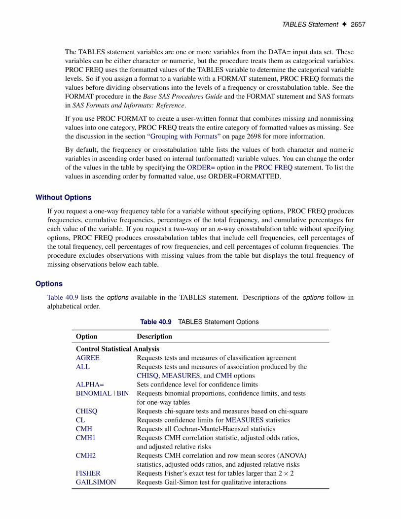
TABLES Statement F 2657
The TABLES statement variables are one or more variables from the DATA= input data set. Thesevariables can be either character or numeric, but the procedure treats them as categorical variables.PROC FREQ uses the formatted values of the TABLES variable to determine the categorical variablelevels. So if you assign a format to a variable with a FORMAT statement, PROC FREQ formats thevalues before dividing observations into the levels of a frequency or crosstabulation table. See theFORMAT procedure in the Base SAS Procedures Guide and the FORMAT statement and SAS formatsin SAS Formats and Informats: Reference.
If you use PROC FORMAT to create a user-written format that combines missing and nonmissingvalues into one category, PROC FREQ treats the entire category of formatted values as missing. Seethe discussion in the section “Grouping with Formats” on page 2698 for more information.
By default, the frequency or crosstabulation table lists the values of both character and numericvariables in ascending order based on internal (unformatted) variable values. You can change the orderof the values in the table by specifying the ORDER= option in the PROC FREQ statement. To list thevalues in ascending order by formatted value, use ORDER=FORMATTED.
Without Options
If you request a one-way frequency table for a variable without specifying options, PROC FREQ producesfrequencies, cumulative frequencies, percentages of the total frequency, and cumulative percentages foreach value of the variable. If you request a two-way or an n-way crosstabulation table without specifyingoptions, PROC FREQ produces crosstabulation tables that include cell frequencies, cell percentages ofthe total frequency, cell percentages of row frequencies, and cell percentages of column frequencies. Theprocedure excludes observations with missing values from the table but displays the total frequency ofmissing observations below each table.
Options
Table 40.9 lists the options available in the TABLES statement. Descriptions of the options follow inalphabetical order.
Table 40.9 TABLES Statement Options
Option Description
Control Statistical AnalysisAGREE Requests tests and measures of classification agreementALL Requests tests and measures of association produced by the
CHISQ, MEASURES, and CMH optionsALPHA= Sets confidence level for confidence limitsBINOMIAL | BIN Requests binomial proportions, confidence limits, and tests
for one-way tablesCHISQ Requests chi-square tests and measures based on chi-squareCL Requests confidence limits for MEASURES statisticsCMH Requests all Cochran-Mantel-Haenszel statisticsCMH1 Requests CMH correlation statistic, adjusted odds ratios,
and adjusted relative risksCMH2 Requests CMH correlation and row mean scores (ANOVA)
statistics, adjusted odds ratios, and adjusted relative risksFISHER Requests Fisher’s exact test for tables larger than 2 � 2GAILSIMON Requests Gail-Simon test for qualitative interactions
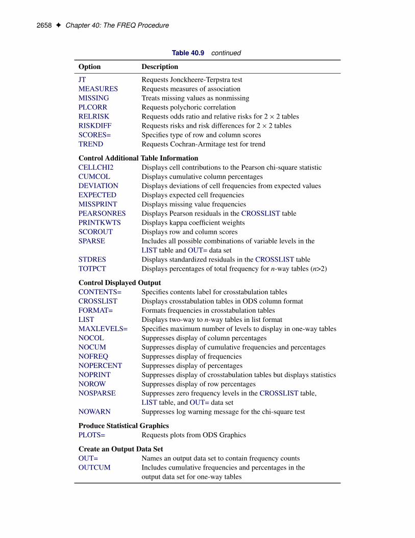
2658 F Chapter 40: The FREQ Procedure
Table 40.9 continued
Option Description
JT Requests Jonckheere-Terpstra testMEASURES Requests measures of associationMISSING Treats missing values as nonmissingPLCORR Requests polychoric correlationRELRISK Requests odds ratio and relative risks for 2 � 2 tablesRISKDIFF Requests risks and risk differences for 2 � 2 tablesSCORES= Specifies type of row and column scoresTREND Requests Cochran-Armitage test for trend
Control Additional Table InformationCELLCHI2 Displays cell contributions to the Pearson chi-square statisticCUMCOL Displays cumulative column percentagesDEVIATION Displays deviations of cell frequencies from expected valuesEXPECTED Displays expected cell frequenciesMISSPRINT Displays missing value frequenciesPEARSONRES Displays Pearson residuals in the CROSSLIST tablePRINTKWTS Displays kappa coefficient weightsSCOROUT Displays row and column scoresSPARSE Includes all possible combinations of variable levels in the
LIST table and OUT= data setSTDRES Displays standardized residuals in the CROSSLIST tableTOTPCT Displays percentages of total frequency for n-way tables (n>2)
Control Displayed OutputCONTENTS= Specifies contents label for crosstabulation tablesCROSSLIST Displays crosstabulation tables in ODS column formatFORMAT= Formats frequencies in crosstabulation tablesLIST Displays two-way to n-way tables in list formatMAXLEVELS= Specifies maximum number of levels to display in one-way tablesNOCOL Suppresses display of column percentagesNOCUM Suppresses display of cumulative frequencies and percentagesNOFREQ Suppresses display of frequenciesNOPERCENT Suppresses display of percentagesNOPRINT Suppresses display of crosstabulation tables but displays statisticsNOROW Suppresses display of row percentagesNOSPARSE Suppresses zero frequency levels in the CROSSLIST table,
LIST table, and OUT= data setNOWARN Suppresses log warning message for the chi-square test
Produce Statistical GraphicsPLOTS= Requests plots from ODS Graphics
Create an Output Data SetOUT= Names an output data set to contain frequency countsOUTCUM Includes cumulative frequencies and percentages in the
output data set for one-way tables
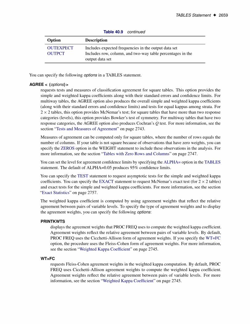
TABLES Statement F 2659
Table 40.9 continued
Option Description
OUTEXPECT Includes expected frequencies in the output data setOUTPCT Includes row, column, and two-way table percentages in the
output data set
You can specify the following options in a TABLES statement.
AGREE < (options) >requests tests and measures of classification agreement for square tables. This option provides thesimple and weighted kappa coefficients along with their standard errors and confidence limits. Formultiway tables, the AGREE option also produces the overall simple and weighted kappa coefficients(along with their standard errors and confidence limits) and tests for equal kappas among strata. For2 � 2 tables, this option provides McNemar’s test; for square tables that have more than two responsecategories (levels), this option provides Bowker’s test of symmetry. For multiway tables that have tworesponse categories, the AGREE option also produces Cochran’s Q test. For more information, see thesection “Tests and Measures of Agreement” on page 2743.
Measures of agreement can be computed only for square tables, where the number of rows equals thenumber of columns. If your table is not square because of observations that have zero weights, you canspecify the ZEROS option in the WEIGHT statement to include these observations in the analysis. Formore information, see the section “Tables with Zero Rows and Columns” on page 2747.
You can set the level for agreement confidence limits by specifying the ALPHA= option in the TABLESstatement. The default of ALPHA=0.05 produces 95% confidence limits.
You can specify the TEST statement to request asymptotic tests for the simple and weighted kappacoefficients. You can specify the EXACT statement to request McNemar’s exact test (for 2 � 2 tables)and exact tests for the simple and weighted kappa coefficients. For more information, see the section“Exact Statistics” on page 2757.
The weighted kappa coefficient is computed by using agreement weights that reflect the relativeagreement between pairs of variable levels. To specify the type of agreement weights and to displaythe agreement weights, you can specify the following options:
PRINTKWTSdisplays the agreement weights that PROC FREQ uses to compute the weighted kappa coefficient.Agreement weights reflect the relative agreement between pairs of variable levels. By default,PROC FREQ uses the Cicchetti-Allison form of agreement weights. If you specify the WT=FCoption, the procedure uses the Fleiss-Cohen form of agreement weights. For more information,see the section “Weighted Kappa Coefficient” on page 2745.
WT=FCrequests Fleiss-Cohen agreement weights in the weighted kappa computation. By default, PROCFREQ uses Cicchetti-Allison agreement weights to compute the weighted kappa coefficient.Agreement weights reflect the relative agreement between pairs of variable levels. For moreinformation, see the section “Weighted Kappa Coefficient” on page 2745.

2660 F Chapter 40: The FREQ Procedure
ALLrequests all tests and measures that are produced by the CHISQ, MEASURES, and CMH options. Youcan control the number of CMH statistics to compute by specifying the CMH1 or CMH2 option.
ALPHA=˛specifies the level of confidence limits. The value of ˛ must be between 0 and 1, and the default is0.05. A confidence level of ˛ produces 100.1 � ˛/% confidence limits. The default of ALPHA=0.05produces 95% confidence limits.
ALPHA= applies to confidence limits that are requested by TABLES statement options. There is aseparate ALPHA= option in the EXACT statement that sets the level of confidence limits for MonteCarlo estimates of exact p-values, which you request by specifying the MC option in the EXACTstatement.
BINOMIAL < (binomial-options) >
BIN < (binomial-options) >requests the binomial proportion for one-way tables. When you specify the BINOMIAL option,by default PROC FREQ also provides the asymptotic standard error, asymptotic Wald and exact(Clopper-Pearson) confidence limits, and the asymptotic equality test for the binomial proportion.
You can specify binomial-options in parentheses after the BINOMIAL option. The LEVEL= binomial-option identifies the variable level for which to compute the proportion. If you do not specify LEVEL=,PROC FREQ computes the proportion for the first level that appears in the output. The P= binomial-option specifies the null proportion for the binomial tests. If you do not specify P=, PROC FREQ usesP=0.5 by default.
You can also specify binomial-options to request additional tests and confidence limits for the binomialproportion. The EQUIV, NONINF, and SUP binomial-options request tests of equivalence, nonin-feriority, and superiority, respectively. The CL= binomial-option requests confidence limits for thebinomial proportion. Table 40.10 summarizes the binomial-options.
Available confidence limits for the binomial proportion include Agresti-Coull, exact (Clopper-Pearson),Jeffreys, Wald, and Wilson (score) confidence limits. You can specify more than one type of binomialconfidence limits in the same analysis. If you do not specify any confidence limit requests, PROCFREQ computes Wald asymptotic confidence limits and exact (Clopper-Pearson) confidence limitsby default. The ALPHA= option determines the confidence level, and the default of ALPHA=0.05produces 95% confidence limits for the binomial proportion.
As part of the noninferiority, superiority, and equivalence analyses, PROC FREQ provides test-basedconfidence limits that have a confidence coefficient of 100.1�2˛/% (Schuirmann 1999). The ALPHA=option determines the confidence level, and the default of ALPHA=0.05 produces 90% confidencelimits. See the sections “Noninferiority Test” on page 2722 and “Equivalence Test” on page 2724 fordetails.
To request exact tests for the binomial proportion, specify the BINOMIAL option in the EXACTstatement. PROC FREQ then computes exact p-values for all binomial tests that you request withbinomial-options, which can include tests of noninferiority, superiority, and equivalence, in addition tothe test of equality.
See the section “Binomial Proportion” on page 2719 for details.
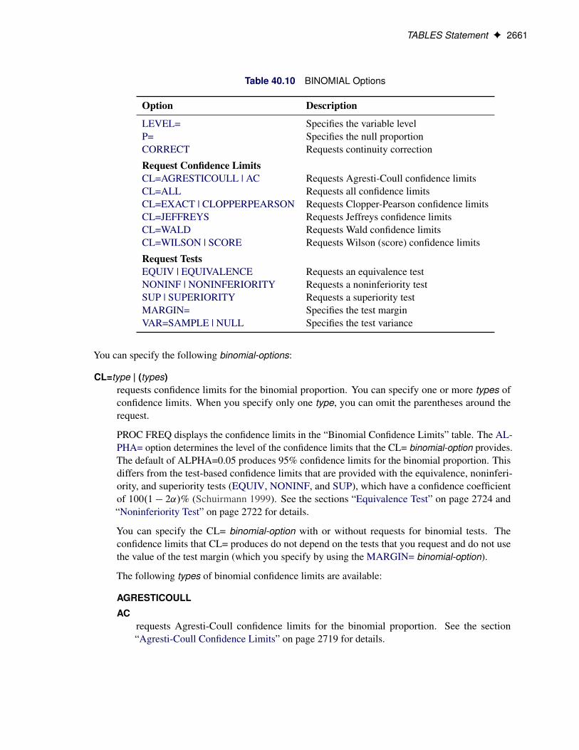
TABLES Statement F 2661
Table 40.10 BINOMIAL Options
Option Description
LEVEL= Specifies the variable levelP= Specifies the null proportionCORRECT Requests continuity correction
Request Confidence LimitsCL=AGRESTICOULL | AC Requests Agresti-Coull confidence limitsCL=ALL Requests all confidence limitsCL=EXACT | CLOPPERPEARSON Requests Clopper-Pearson confidence limitsCL=JEFFREYS Requests Jeffreys confidence limitsCL=WALD Requests Wald confidence limitsCL=WILSON | SCORE Requests Wilson (score) confidence limits
Request TestsEQUIV | EQUIVALENCE Requests an equivalence testNONINF | NONINFERIORITY Requests a noninferiority testSUP | SUPERIORITY Requests a superiority testMARGIN= Specifies the test marginVAR=SAMPLE | NULL Specifies the test variance
You can specify the following binomial-options:
CL=type | (types)requests confidence limits for the binomial proportion. You can specify one or more types ofconfidence limits. When you specify only one type, you can omit the parentheses around therequest.
PROC FREQ displays the confidence limits in the “Binomial Confidence Limits” table. The AL-PHA= option determines the level of the confidence limits that the CL= binomial-option provides.The default of ALPHA=0.05 produces 95% confidence limits for the binomial proportion. Thisdiffers from the test-based confidence limits that are provided with the equivalence, noninferi-ority, and superiority tests (EQUIV, NONINF, and SUP), which have a confidence coefficientof 100.1 � 2˛/% (Schuirmann 1999). See the sections “Equivalence Test” on page 2724 and“Noninferiority Test” on page 2722 for details.
You can specify the CL= binomial-option with or without requests for binomial tests. Theconfidence limits that CL= produces do not depend on the tests that you request and do not usethe value of the test margin (which you specify by using the MARGIN= binomial-option).
The following types of binomial confidence limits are available:
AGRESTICOULL
ACrequests Agresti-Coull confidence limits for the binomial proportion. See the section“Agresti-Coull Confidence Limits” on page 2719 for details.
2662 F Chapter 40: The FREQ Procedure
ALLrequests all available types of confidence limits for the binomial proportion. These includethe following: Agresti-Coull, exact (Clopper-Pearson), Jeffreys, Wald, and Wilson (score)confidence limits.
EXACT
CLOPPERPEARSONrequests exact (Clopper-Pearson) confidence limits for the binomial proportion. See thesection “Exact (Clopper-Pearson) Confidence Limits” on page 2720 for details. If you do notrequest any binomial confidence limits by specifying the CL= binomial-option, PROC FREQproduces Wald and exact (Clopper-Pearson) confidence limits by default. To request exacttests for the binomial proportion, specify the BINOMIAL option in the EXACT statement.
JEFFREYSrequests Jeffreys confidence limits for the binomial proportion. See the section “JeffreysConfidence Limits” on page 2720 for details.
WALD < (CORRECT) >requests Wald confidence limits for the binomial proportion. See the section “Wald Con-fidence Limits” on page 2719 for details. If you do not request any binomial confidencelimits by specifying the CL= binomial-option, PROC FREQ produces Wald and exact(Clopper-Pearson) confidence limits by default.
If you specify CL=WALD(CORRECT), the Wald confidence limits include a continuitycorrection. If you specify the CORRECT binomial-option, the Wald confidence limits andthe Wald tests include continuity corrections.
WILSON < (CORRECT) >
SCORE < (CORRECT) >requests Wilson confidence limits for the binomial proportion. These are also known asscore confidence limits. See the section “Wilson (Score) Confidence Limits” on page 2720for details.
If you specify CL=WILSON(CORRECT) or the CORRECT binomial-option, the Wilsonconfidence limits include a continuity correction.
CORRECTincludes a continuity correction in the Wald confidence limits, Wald tests, and Wilson confidencelimits.
You can request continuity corrections individually for Wald or Wilson confidence limits by spec-ifying the CL=WALD(CORRECT) or CL=WILSON(CORRECT) binomial-option, respectively.
EQUIV
EQUIVALENCErequests a test of equivalence for the binomial proportion. See the section “Equivalence Test” onpage 2724 for details. You can specify the equivalence test margins, the null proportion, and thevariance type with the MARGIN=, P=, and VAR= binomial-options, respectively. To request anexact equivalence test, specify the BINOMIAL option in the EXACT statement.
TABLES Statement F 2663
LEVEL=level-number | ‘level-value’specifies the variable level for the binomial proportion. By default, PROC FREQ computesthe proportion of observations for the first variable level that appears in the output. To requesta different level, use LEVEL=level-number or LEVEL=‘level-value’, where level-number isthe variable level’s number or order in the output, and level-value is the formatted value of thevariable level. The value of level-number must be a positive integer. You must enclose level-valuein single quotes.
MARGIN=value | (lower , upper )specifies the margin for the noninferiority, superiority, and equivalence tests, which you requestwith the NONINF, SUP, and EQUIV binomial-options, respectively. If you do not specify thisoption, PROC FREQ uses a margin of 0.2 by default.
For noninferiority and superiority tests, specify a single value for the MARGIN= option. TheMARGIN= value must be a positive number. You can specify value as a number between 0 and 1.Or you can specify value in percentage form as a number between 1 and 100, and PROC FREQconverts that number to a proportion. The procedure treats the value 1 as 1%.
For noninferiority and superiority tests, the test limits must be between 0 and 1. The limits aredetermined by the null proportion value (which you can specify with the P= binomial-option) andby the margin value. The noninferiority limit equals the null proportion minus the margin. Bydefault, the null proportion equals 0.5 and the margin equals 0.2, which gives a noninferioritylimit of 0.3. The superiority limit equals the null proportion plus the margin, which is 0.7 bydefault.
For an equivalence test, you can specify a single MARGIN= value, or you can specify both lowerand upper values. If you specify a single MARGIN= value, it must be a positive number, asdescribed previously. If you specify a single MARGIN= value for an equivalence test, PROCFREQ uses –value as the lower margin and value as the upper margin for the test. If you specifyboth lower and upper values for an equivalence test, you can specify them in proportion form asnumbers between –1 or 1. Or you can specify them in percentage form as numbers between –100and 100, and PROC FREQ converts the numbers to proportions. The value of lower must be lessthan the value of upper .
The equivalence limits must be between 0 and 1. The equivalence limits are determined by thenull proportion value (which you can specify with the P= binomial-option) and by the marginvalues. The lower equivalence limit equals the null proportion plus the lower margin. By default,the null proportion equals 0.5 and the lower margin equals –0.2, which gives a lower equivalencelimit of 0.3. The upper equivalence limit equals the null proportion plus the upper margin, whichis 0.7 by default.
See the sections “Noninferiority Test” on page 2722 and “Equivalence Test” on page 2724 fordetails.
NONINF
NONINFERIORITYrequests a test of noninferiority for the binomial proportion. See the section “Noninferiority Test”on page 2722 for details. You can specify the noninferiority test margin, the null proportion, andthe variance type with the MARGIN=, P=, and VAR= binomial-options, respectively. To requestan exact noninferiority test, specify the BINOMIAL option in the EXACT statement.
2664 F Chapter 40: The FREQ Procedure
P=valuespecifies the null hypothesis proportion for the binomial tests. If you omit this option, PROCFREQ uses 0.5 as the null proportion. The null proportion value must be a positive number. Youcan specify value as a number between 0 and 1. Or you can specify value in percentage formas a number between 1 and 100, and PROC FREQ converts that number to a proportion. Theprocedure treats the value 1 as 1%.
SUP
SUPERIORITYrequests a test of superiority for the binomial proportion. See the section “Superiority Test” onpage 2723 for details. You can specify the superiority test margin, the null proportion, and thevariance type with the MARGIN=, P=, and VAR= binomial-options, respectively. To request anexact superiority test, specify the BINOMIAL option in the EXACT statement.
VAR=SAMPLE | NULLspecifies the type of variance estimate to use in the Wald tests of noninferiority, superiority,and equivalence. The default is VAR=SAMPLE, which estimates the variance from the sampleproportion. VAR=NULL uses a test-based variance that is computed from the null hypothesisproportion (which is specified by the P= binomial-option). See the sections “Noninferiority Test”on page 2722 and “Equivalence Test” on page 2724 for details.
CELLCHI2displays each table cell’s contribution to the Pearson chi-square statistic in the crosstabulation table.The cell chi-square is computed as .frequency � expected/2=expected, where frequency is the tablecell frequency (count) and expected is the expected cell frequency, which is computed under the nullhypothesis that the row and column variables are independent. For more information, see the section“Pearson Chi-Square Test for Two-Way Tables” on page 2705. This option has no effect for one-waytables or for tables that are displayed in list format (which you can request by specifying the LISToption).
CHISQ < (chisq-options) >requests chi-square tests of homogeneity or independence and measures of association that are basedon the chi-square statistic. For two-way tables, the chi-square tests include the Pearson chi-square,likelihood ratio chi-square, and Mantel-Haenszel chi-square tests. The chi-square measures includethe phi coefficient, contingency coefficient, and Cramér’s V. For 2 � 2 tables, the CHISQ option alsoprovides Fisher’s exact test and the continuity-adjusted chi-square test. See the section “Chi-SquareTests and Statistics” on page 2704 for details.
For one-way tables, the CHISQ option provides the Pearson chi-square goodness-of-fit test. Youcan also request the likelihood ratio goodness-of-fit test for one-way tables by specifying the LRCHIchisq-option in parentheses after the CHISQ option. By default, the one-way chi-square tests arebased on the null hypothesis of equal proportions. Alternatively, you can provide null hypothesisproportions or frequencies by specifying the TESTP= or TESTF= chisq-option, respectively. See thesection “Chi-Square Test for One-Way Tables” on page 2704 for more information.
To request Fisher’s exact test for tables larger than 2 � 2, specify the FISHER option in the EXACTstatement. Exact p-values are also available for the Pearson, likelihood ratio, and Mantel-Haenszelchi-square tests. See the description of the EXACT statement for more information.

TABLES Statement F 2665
You can specify the following chisq-options:
DF=dfspecifies the degrees of freedom for the chi-square tests. The value of df must not be zero. If thevalue of df is positive, PROC FREQ uses df as the degrees of freedom for the chi-square tests. Ifthe value of df is negative, PROC FREQ uses df to adjust the default degrees of freedom for thechi-square tests.
By default for one-way tables, the value of df is (n – 1), where n is the number of variable levelsin the table. By default for two-way tables, the value of df is (r – 1) (c – 1), where r is thenumber of rows in the table and c is the number of columns. See the sections “Chi-Square Testfor One-Way Tables” on page 2704 and “Chi-Square Tests and Statistics” on page 2704 for moreinformation.
If you specify a negative value of df , PROC FREQ adjusts the default degrees of freedom byadding the (negative) value of df to the default value to produce the adjusted degrees of freedom.The adjusted degrees of freedom must be positive.
The DF= chisq-option specifies or adjusts the degrees of freedom for the following chi-squaretests: the Pearson and likelihood ratio goodness-of-fit tests for one-way tables; and the Pearson,likelihood ratio, and Mantel-Haenszel chi-square tests for two-way tables.
LRCHIrequests the likelihood ratio goodness-of-fit test for one-way tables. See the section “LikelihoodRatio Chi-Square Test for One-Way Tables” on page 2706 for more information.
By default, this test is based on the null hypothesis of equal proportions. You can providenull hypothesis proportions or frequencies by specifying the TESTP= or TESTF= chisq-option,respectively. You can request an exact likelihood ratio goodness-of-fit test by specifying theLRCHI option in the EXACT statement.
TESTF=(values)| SAS-data-setspecifies null hypothesis frequencies for the one-way chi-square goodness-of-fit tests. See thesection “Chi-Square Test for One-Way Tables” on page 2704 for details. You can list the nullfrequencies as values in parentheses after TESTF=. Or you can provide the null frequencies in asecondary input data set by specifying TESTF=SAS-data-set . The TESTF=SAS-data-set cannotbe the same data set that you specify in the DATA= option. You can specify only one TESTF= orTESTP= data set in a single invocation of the procedure.
If you list the null frequencies as values, you can separate the values with blanks or commas.The values must be positive numbers. The number of values must equal the number of variablelevels in the one-way table. The sum of the values must equal the total frequency for the one-waytable. Order the values to match the order in which the corresponding variable levels appear inthe one-way frequency table.
If you provide the null frequencies in a secondary input data set (TESTF=SAS-data-set), the vari-able that contains the null frequencies should be named _TESTF_, TestFrequency, or Frequency.The null frequencies must be positive numbers. The number of frequencies must equal thenumber of levels in the one-way frequency table, and the sum of the frequencies must equal thetotal frequency for the one-way table. Order the null frequencies in the data set to match theorder in which the corresponding variable levels appear in the one-way frequency table.
2666 F Chapter 40: The FREQ Procedure
TESTP=(values)| SAS-data-setspecifies null hypothesis proportions for the one-way chi-square goodness-of-fit tests. See thesection “Chi-Square Test for One-Way Tables” on page 2704 for details. You can list the nullproportions as values in parentheses after TESTP=. Or you can provide the null proportions in asecondary input data set by specifying TESTP=SAS-data-set . The TESTP=SAS-data-set cannotbe the same data set that you specify in the DATA= option. You can specify only one TESTF= orTESTP= data set in a single invocation of the procedure.
If you list the null proportions as values, you can separate the values with blanks or commas.The values must be positive numbers. The number of values must equal the number of variablelevels in the one-way table. Order the values to match the order in which the correspondingvariable levels appear in the one-way frequency table. You can specify values in probabilityform as numbers between 0 and 1, where the proportions sum to 1. Or you can specify values inpercentage form as numbers between 0 and 100, where the percentages sum to 100.
If you provide the null proportions in a secondary input data set (TESTP=SAS-data-set), thevariable that contains the null proportions should be named _TESTP_, TestPercent, or Percent.The null proportions must be positive numbers. The number of proportions must equal thenumber of levels in the one-way frequency table. You can provide the proportions in probabilityform as numbers between 0 and 1, where the proportions sum to 1. Or you can provide theproportions in percentage form as numbers between 0 and 100, where the percentages sum to100. Order the null proportions in the data set to match the order in which the correspondingvariable levels appear in the one-way frequency table.
WARN=type | (types)controls the warning message for the validity of the asymptotic Pearson chi-square test. Bydefault, PROC FREQ displays a warning message when more than 20% of the table cells haveexpected frequencies that are less than 5. If you specify the NOPRINT option in the PROC FREQstatement, the procedure displays the warning in the log; otherwise, the procedure displays thewarning as a footnote in the chi-square table. You can use the WARN= option to suppress thewarning and to include a warning indicator in the output data set.
You can specify one or more of the following types in the WARN= option. If you specifymore than one type value, enclose the values in parentheses after WARN=. For example,warn = (output noprint).
Value of WARN= Description
OUTPUT Adds a warning indicator variable to the output data setNOLOG Suppresses the chi-square warning message in the logNOPRINT Suppresses the chi-square warning message in the displayNONE Suppresses the chi-square warning message entirely
If you specify the WARN=OUTPUT option, the ODS output data set ChiSq contains a variablenamed Warning that equals 1 for the Pearson chi-square observation when more than 20% of thetable cells have expected frequencies that are less than 5 and equals 0 otherwise. If you specifyWARN=OUTPUT and also specify the CHISQ option in the OUTPUT statement, the statisticsoutput data set contains a variable named WARN_PCHI that indicates the warning.
The WARN=NOLOG option has the same effect as the NOWARN option in the TABLESstatement.
TABLES Statement F 2667
CLrequests confidence limits for the measures of association, which you can request by specifying theMEASURES option. For more information, see the sections “Measures of Association” on page 2709and “Confidence Limits” on page 2710. You can set the level of the confidence limits by using theALPHA= option. The default of ALPHA=0.05 produces 95% confidence limits.
If you omit the MEASURES option, the CL option invokes MEASURES. The CL option is equivalentto the MEASURES(CL) option.
CMH < (cmh-options) >requests Cochran-Mantel-Haenszel statistics, which test for association between the row and columnvariables after adjusting for the remaining variables in a multiway table. The Cochran-Mantel-Haenszelstatistics include the nonzero correlation statistic, the row mean scores (ANOVA) statistic, and thegeneral association statistic. In addition, for 2 � 2 tables, the CMH option provides the adjustedMantel-Haenszel and logit estimates of the odds ratio and relative risks, together with their confidencelimits. For stratified 2 � 2 tables, the CMH option provides the Breslow-Day test for homogeneity ofodds ratios. (To request Tarone’s adjustment for the Breslow-Day test, specify the BDT cmh-option.)See the section “Cochran-Mantel-Haenszel Statistics” on page 2748 for details.
You can use the CMH1 or CMH2 option to control the number of CMH statistics that PROC FREQcomputes.
For stratified 2 � 2 tables, you can request Zelen’s exact test for equal odds ratios by specifying theEQOR option in the EXACT statement. See the section “Zelen’s Exact Test for Equal Odds Ratios” onpage 2754 for details. You can request exact confidence limits for the common odds ratio by specifyingthe COMOR option in the EXACT statement. This option also provides a common odds ratio test. Seethe section “Exact Confidence Limits for the Common Odds Ratio” on page 2754 for details.
You can specify the following cmh-options in parentheses after the CMH option. These cmh-options,which apply to stratified 2 � 2 tables, are also available with the CMH1 or CMH2 option.
BDTrequests Tarone’s adjustment in the Breslow-Day test for homogeneity of odds ratios. See thesection “Breslow-Day Test for Homogeneity of the Odds Ratios” on page 2753 for details.
GAILSIMON < (COLUMN=1 | 2) >
GS < (COLUMN=1 | 2) >requests the Gail-Simon test for qualitative interaction, which applies to stratified 2 � 2 tables.See the section “Gail-Simon Test for Qualitative Interactions” on page 2756 for details.
The COLUMN= option specifies the column of the risk differences to use in computing the Gail-Simon test. By default, PROC FREQ uses column 1 risk differences. If you specify COLUMN=2,PROC FREQ uses column 2 risk differences.
The GAILSIMON cmh-option has the same effect as the GAILSIMON option in the TABLESstatement.
MANTELFLEISS
MFrequests the Mantel-Fleiss criterion for the Mantel-Haenszel statistic for stratified 2 � 2 tables.See the section “Mantel-Fleiss Criterion” on page 2751 for details.

2668 F Chapter 40: The FREQ Procedure
CMH1 < (cmh-options) >requests the Cochran-Mantel-Haenszel correlation statistic. This option does not provide the CMH rowmean scores (ANOVA) statistic or the general association statistic, which are provided by the CMHoption. For tables larger than 2 � 2, the CMH1 option requires less memory than the CMH option,which can require an enormous amount of memory for large tables.
For 2 � 2 tables, the CMH1 option also provides the adjusted Mantel-Haenszel and logit estimates ofthe odds ratio and relative risks, together with their confidence limits. For stratified 2 � 2 tables, theCMH1 option provides the Breslow-Day test for homogeneity of odds ratios.
The cmh-options for CMH1 are the same as the cmh-options that are available with the CMH option.See the description of the CMH option for details.
CMH2 < (cmh-options) >requests the Cochran-Mantel-Haenszel correlation statistic and the row mean scores (ANOVA) statistic.This option does not provide the CMH general association statistic, which is provided by the CMHoption. For tables larger than 2 � 2, the CMH2 option requires less memory than the CMH option,which can require an enormous amount of memory for large tables.
For 2 � 2 tables, the CMH1 option also provides the adjusted Mantel-Haenszel and logit estimates ofthe odds ratio and relative risks, together with their confidence limits. For stratified 2 � 2 tables, theCMH1 option provides the Breslow-Day test for homogeneity of odds ratios.
The cmh-options for CMH2 are the same as the cmh-options that are available with the CMH option.See the description of the CMH option for details.
CONTENTS=‘string’specifies the label to use for crosstabulation tables in the contents file, the Results window, and thetrace record. For information about output presentation, see the SAS Output Delivery System: User’sGuide.
If you omit the CONTENTS= option, the contents label for crosstabulation tables is “Cross-TabularFreq Table” by default.
Note that contents labels for all crosstabulation tables that are produced by a single TABLES statementuse the same text. To specify different contents labels for different crosstabulation tables, request thetables in separate TABLES statements and use the CONTENTS= option in each TABLES statement.
To remove the crosstabulation table entry from the contents file, you can specify a null label withCONTENTS=‘’ .
The CONTENTS= option affects only contents labels for crosstabulation tables. It does not affectcontents labels for other PROC FREQ tables.
To specify the contents label for any PROC FREQ table, you can use PROC TEMPLATE to createa customized table template. The CONTENTS_LABEL attribute in the DEFINE TABLE statementof PROC TEMPLATE specifies the contents label for the table. See the chapter “The TEMPLATEProcedure” in the SAS Output Delivery System: User’s Guide for more information.
CROSSLIST < (options) >displays crosstabulation tables by using an ODS column format instead of the default crosstabulationcell format. In the CROSSLIST table display, the rows correspond to the crosstabulation table cells, andthe columns correspond to descriptive statistics such as frequencies and percentages. The CROSSLIST

TABLES Statement F 2669
table displays the same information as the default crosstabulation table (but it uses an ODS columnformat). For more information about the contents of the CROSSLIST table, See the section “Two-Wayand Multiway Tables” on page 2767.
You can control the contents of a CROSSLIST table by specifying the same options available for thedefault crosstabulation table. These include the NOFREQ, NOPERCENT, NOROW, and NOCOLoptions. You can request additional information in a CROSSLIST table by specifying the CELLCHI2,DEVIATION, EXPECTED, MISSPRINT, and TOTPCT options. You can also display standardizedresiduals or Pearson residuals in a CROSSLIST table by specifying the CROSSLIST(STDRES) orCROSSLIST(PEARSONRES) option, respectively; these options are not available for the defaultcrosstabulation table. The FORMAT= and CUMCOL options have no effect on CROSSLIST tables.You cannot specify both the LIST option and the CROSSLIST option in the same TABLES statement.
For CROSSLIST tables, you can use the NOSPARSE option to suppress display of variable levels thathave zero frequencies. By default, PROC FREQ displays all levels of the column variable within eachlevel of the row variable, including any levels that have zero frequencies. By default for multiwaytables that are displayed as CROSSLIST tables, the procedure displays all levels of the row variablefor each stratum of the table, including any row levels with zero frequencies in the stratum.
You can specify the following options:
STDRESdisplays the standardized residuals of the table cells in the CROSSLIST table. The standardizedresidual is the ratio of (frequency – expected) to its standard error, where frequency is the tablecell frequency (count) and expected is the expected table cell frequency, which is computed underthe null hypothesis that the row and column variables are independent. For more information, seethe section “Standardized Residuals” on page 2705. You can display the expected values anddeviations by specifying the EXPECTED and DEVIATION options, respectively.
PEARSONRESdisplays the Pearson residuals of the table cells in the CROSSLIST table. The Pearson residual isthe square root of the table cell’s contribution to the Pearson chi-square statistic. The Pearsonresidual is computed as .frequency � expected/=
pexpected, where frequency is the table cell
frequency (count) and expected is the expected table cell frequency, which is computed under thenull hypothesis that the row and column variables are independent. For more information, seethe section “Pearson Chi-Square Test for Two-Way Tables” on page 2705. You can display theexpected values, deviations, and cell chi-squares by specifying the EXPECTED, DEVIATION,and CELLCHI2 options, respectively.
CUMCOLdisplays the cumulative column percentages in the cells of the crosstabulation table. The CUMCOLoption does not apply to crosstabulation tables produced with the LIST or CROSSLIST option.
DEVIATIONdisplays the deviations of the frequencies from the expected frequencies (frequency – expected) in thecrosstabulation table. The expected frequencies are computed under the null hypothesis that the rowand column variables are independent. For more information, see the section “Pearson Chi-SquareTest for Two-Way Tables” on page 2705. You can display the expected values by specifying theEXPECTED option. This option has no effect for one-way tables or for tables that are displayed in listformat (which you can request by specifying the LIST option).
2670 F Chapter 40: The FREQ Procedure
EXPECTEDdisplays the expected cell frequencies in the crosstabulation table. The expected frequencies arecomputed under the null hypothesis that the row and column variables are independent. For moreinformation, see the section “Pearson Chi-Square Test for Two-Way Tables” on page 2705. This optionhas no effect for one-way tables or for tables that are displayed in list format (which you can requestby specifying the LIST option).
FISHERrequests Fisher’s exact test for tables that are larger than 2 � 2. (For 2 � 2 tables, the CHISQ optionprovides Fisher’s exact test.) This test is also known as the Freeman-Halton test. See the sections“Fisher’s Exact Test” on page 2708 and “Exact Statistics” on page 2757 for more information.
If you omit the CHISQ option in the TABLES statement, the FISHER option invokes CHISQ. You canalso request Fisher’s exact test by specifying the FISHER option in the EXACT statement.
NOTE: PROC FREQ computes exact tests by using fast and efficient algorithms that are superior todirect enumeration. Exact tests are appropriate when a data set is small, sparse, skewed, or heavilytied. For some large problems, computation of exact tests might require a substantial amount of timeand memory. Consider using asymptotic tests for such problems. Alternatively, when asymptoticmethods might not be sufficient for such large problems, consider using Monte Carlo estimation ofexact p-values. You can request Monte Carlo estimation by specifying the MC computation-option inthe EXACT statement. See the section “Computational Resources” on page 2759 for more information.
FORMAT=format-namespecifies a format for the following crosstabulation table cell values: frequency, expected frequency,and deviation. PROC FREQ also uses the specified format to display the row and column totalfrequencies and the overall total frequency in crosstabulation tables.
You can specify any standard SAS numeric format or a numeric format defined with the FORMATprocedure. The format length must not exceed 24. If you omit the FORMAT= option, by default PROCFREQ uses the BEST6. format to display frequencies less than 1E6, and the BEST7. format otherwise.
The FORMAT= option applies only to crosstabulation tables displayed in the default format. It doesnot apply to crosstabulation tables produced with the LIST or CROSSLIST option.
To change display formats in any FREQ table, you can use PROC TEMPLATE. See the chapter “TheTEMPLATE Procedure” in the SAS Output Delivery System: User’s Guide for more information.
GAILSIMON < (COLUMN=1 | 2) >
GS < (COLUMN=1 | 2) >requests the Gail-Simon test for qualitative interaction, which applies to stratified 2 � 2 tables. See thesection “Gail-Simon Test for Qualitative Interactions” on page 2756 for details.
The COLUMN= option specifies the column of the risk differences to use in computing the Gail-Simontest. By default, PROC FREQ uses column 1 risk differences. If you specify COLUMN=2, PROCFREQ uses column 2 risk differences.
JTrequests the Jonckheere-Terpstra test. See the section “Jonckheere-Terpstra Test” on page 2741 fordetails. To request exact p-values for the Jonckheere-Terpstra test, specify the JT option in the EXACTstatement. See the section “Exact Statistics” on page 2757 for more information.

TABLES Statement F 2671
LISTdisplays two-way and multiway tables by using a list format instead of the default crosstabulation cellformat. This option displays an entire multiway table in one table, instead of displaying a separatetwo-way table for each stratum. For more information, see the section “Two-Way and Multiway Tables”on page 2767.
The LIST option is not available when you request tests and statistics; you must use the standardcrosstabulation table display or the CROSSLIST display when you request tests and statistics.
MAXLEVELS=nspecifies the maximum number of variable levels to display in one-way frequency tables. The value ofn must be a positive integer. PROC FREQ displays the first n variable levels, matching the order inwhich the levels appear in the one-way frequency table. (The ORDER= option controls the order ofthe variable levels. By default, ORDER=INTERNAL, which orders the variable levels by unformattedvalue.)
The MAXLEVELS= option also applies to one-way frequency plots, which you can request byspecifying the PLOTS=FREQPLOT option when ODS Graphics is enabled.
If you specify the MISSPRINT option to display missing levels in the frequency table, theMAXLEVELS= option displays the first n nonmissing levels.
The MAXLEVELS= option does not apply to the OUT= output data set, which includes all variablelevels. The MAXLEVELS= option does not affect the computation of percentages, statistics, or testsfor the one-way table; these values are based on the complete table.
MEASURES < (CL) >requests measures of association and their asymptotic standard errors. This option provides thefollowing measures: gamma, Kendall’s tau-b, Stuart’s tau-c, Somers’ D.C jR/, Somers’ D.RjC/,Pearson and Spearman correlation coefficients, lambda (symmetric and asymmetric), and uncertaintycoefficients (symmetric and asymmetric). If you specify the CL option in parentheses after theMEASURES option, PROC FREQ provides confidence limits for the measures of association. Formore information, see the section “Measures of Association” on page 2709.
For 2� 2 tables, the MEASURES option also provides the odds ratio, column 1 relative risk, column 2relative risk, and their asymptotic Wald confidence limits. You can request the odds ratio and relativerisks separately (without the other measures of association) by specifying the RELRISK option. Youcan request confidence limits for the odds ratio by specifying the OR(CL=) option.
You can use the TEST statement to request asymptotic tests for the following measures of association:gamma, Kendall’s tau-b, Stuart’s tau-c, Somers’ D.C jR/, Somers’ D.RjC/, and Pearson and Spear-man correlation coefficients. You can use the EXACT statement to request exact confidence limitsfor the odds ratio, exact unconditional confidence limits for the relative risks, and exact tests for thefollowing measures of association: Kendall’s tau-b, Stuart’s tau-c, Somers’ D.C jR/ and D.RjC/, andPearson and Spearman correlation coefficients. For more information, see the descriptions of the TESTand EXACT statements and the section “Exact Statistics” on page 2757.
MISSINGtreats missing values as a valid nonmissing level for all TABLES variables. The MISSING optiondisplays the missing levels in frequency and crosstabulation tables and includes them in all calculationsof percentages, tests, and measures.
2672 F Chapter 40: The FREQ Procedure
By default, if you do not specify the MISSING or MISSPRINT option, an observation is excluded froma table if it has a missing value for any of the variables in the TABLES request. When PROC FREQexcludes observations with missing values, it displays the total frequency of missing observationsbelow the table. See the section “Missing Values” on page 2699 for more information.
MISSPRINTdisplays missing value frequencies in frequency and crosstabulation tables but does not include themissing value frequencies in any computations of percentages, tests, or measures.
By default, if you do not specify the MISSING or MISSPRINT option, an observation is excluded froma table if it has a missing value for any of the variables in the TABLES request. When PROC FREQexcludes observations with missing values, it displays the total frequency of missing observationsbelow the table. See the section “Missing Values” on page 2699 for more information.
NOCOLsuppresses the display of column percentages in crosstabulation table cells.
NOCUMsuppresses the display of cumulative frequencies and percentages in one-way frequency tables. TheNOCUM option also suppresses the display of cumulative frequencies and percentages in crosstabula-tion tables in list format, which you request with the LIST option.
NOFREQsuppresses the display of cell frequencies in crosstabulation tables. The NOFREQ option also sup-presses row total frequencies. This option has no effect for one-way tables or for crosstabulation tablesin list format, which you request with the LIST option.
NOPERCENTsuppresses the display of overall percentages in crosstabulation tables. These percentages include thecell percentages of the total (two-way) table frequency, as well as the row and column percentages ofthe total table frequency. To suppress the display of cell percentages of row or column totals, use theNOROW or NOCOL option, respectively.
For one-way frequency tables and crosstabulation tables in list format, the NOPERCENT optionsuppresses the display of percentages and cumulative percentages.
NOPRINTsuppresses the display of frequency and crosstabulation tables but displays all requested tests andstatistics. To suppress the display of all output, including tests and statistics, use the NOPRINT optionin the PROC FREQ statement.
NOROWsuppresses the display of row percentages in crosstabulation table cells.
NOSPARSEsuppresses the display of cells with a zero frequency count in LIST output and omits them fromthe OUT= data set. The NOSPARSE option applies when you specify the ZEROS option in theWEIGHT statement to include observations with zero weights. By default, the ZEROS option invokesthe SPARSE option, which displays table cells with a zero frequency count in the LIST output andincludes them in the OUT= data set. See the description of the ZEROS option for more information.

TABLES Statement F 2673
The NOSPARSE option also suppresses the display of variable levels with zero frequency inCROSSLIST tables. By default for CROSSLIST tables, PROC FREQ displays all levels of thecolumn variable within each level of the row variable, including any column variable levels with zerofrequency for that row. For multiway tables displayed with the CROSSLIST option, the proceduredisplays all levels of the row variable for each stratum of the table by default, including any rowvariable levels with zero frequency for the stratum.
NOWARNsuppresses the log warning message for the validity of the asymptotic Pearson chi-square test. Bydefault, PROC FREQ provides a validity warning for the asymptotic Pearson chi-square test whenmore than 20cells have expected frequencies that are less than 5. This warning message appears in thelog if you specify the NOPRINT option in the PROC FREQ statement,
The NOWARN option is equivalent to the CHISQ(WARN=NOLOG) option. You can also use theCHISQ(WARN=) option to suppress the warning message in the display and to request a warningvariable in the chi-square ODS output data set or in the OUTPUT data set.
OR(CL=type | (types))
ODDSRATIO(CL=type | (types))requests the odds ratio and confidence limits for 2 � 2 tables. You can specify one or more types ofconfidence limits, which include exact, score, and Wald confidence limits. When you specify only oneconfidence limit type, you can omit the parentheses around the request.
PROC FREQ displays the confidence limits in the “Confidence Limits for the Odds Ratio” table.Specifying the OR option without the CL= option is equivalent to specifying the RELRISK option,which produces the “Odds Ratio and Relative Risks” table. For more information, see the descriptionof the RELRISK option. When you specify the OR(CL=) option, PROC FREQ does not produce the“Odds Ratio and Relative Risks” table unless you also specify the RELRISK or MEASURES option.
The ALPHA= option determines the confidence level, and the default of ALPHA=0.05 produces 95%confidence limits for the odds ratio.
You can specify the following types:
EXACTdisplays exact confidence limits for the odds ratio in the “Confidence Limits for the Odds Ratio”table. You must also request computation of the exact confidence limits by specifying the ORoption in the EXACT statement. For more information, see the section “Exact Confidence Limitsfor the Odds Ratio” on page 2738.
SCORE < (CORRECT=NO) >requests score confidence limits for the odds ratio. For more information, see the section “ScoreConfidence Limits for the Odds Ratio” on page 2738. If you specify CORRECT=NO, PROCFREQ provides the uncorrected form of the confidence limits.
WALDrequests asymptotic Wald confidence limits for the odds ratio. For more information, see thesection “Odds Ratio and Relative Risks for 2 x 2 Tables” on page 2737.

2674 F Chapter 40: The FREQ Procedure
OUT=SAS-data-setnames an output data set that contains frequency or crosstabulation table counts and percentages. Ifmore than one table request appears in the TABLES statement, the contents of the OUT= data setcorrespond to the last table request in the TABLES statement. The OUT= data set variable COUNTcontains the frequencies and the variable PERCENT contains the percentages. See the section “OutputData Sets” on page 2762 for details. You can specify the following options to include additionalinformation in the OUT= data set: OUTCUM, OUTEXPECT, and OUTPCT.
OUTCUMincludes cumulative frequencies and cumulative percentages in the OUT= data set for one-way tables.The variable CUM_FREQ contains the cumulative frequencies, and the variable CUM_PCT contains thecumulative percentages. See the section “Output Data Sets” on page 2762 for details. The OUTCUMoption has no effect for two-way or multiway tables.
OUTEXPECTincludes expected cell frequencies in the OUT= data set for crosstabulation tables. The variableEXPECTED contains the expected cell frequencies. See the section “Output Data Sets” on page 2762for details. The EXPECTED option has no effect for one-way tables.
OUTPCTincludes the following additional variables in the OUT= data set for crosstabulation tables:
PCT_COL percentage of column frequency
PCT_ROW percentage of row frequency
PCT_TABL percentage of stratum (two-way table) frequency, for n-way tables where n > 2
See the section “Output Data Sets” on page 2762 for details. The OUTPCT option has no effect forone-way tables.
PLCORR < (options) >requests the polychoric correlation coefficient and its asymptotic standard error. For 2 � 2 tables, thisstatistic is more commonly known as the tetrachoric correlation coefficient, and it is labeled as such inthe displayed output. For more information, see the section “Polychoric Correlation” on page 2715.
If you also specify the CL or MEASURES(CL) option, PROC FREQ provides confidence limits forthe polychoric correlation. If you specify the PLCORR option in the TEST statement, the procedureprovides Wald and likelihood ratio tests for the polychoric correlation. The PLCORR option invokesthe MEASURES option.
You can specify the following options:
CONVERGE=valuespecifies the convergence criterion for computing the polychoric correlation. The convergencecriterion value must be a positive number. By default, CONVERGE=0.0001. Iterative com-putation of the polychoric correlation stops when the convergence measure falls below valueor when the number of iterations exceeds the MAXITER= number , whichever happens first.For parameter values that are less than 0.01, PROC FREQ evaluates convergence by using theabsolute difference instead of the relative difference. For more information, see the section“Polychoric Correlation” on page 2715.
TABLES Statement F 2675
MAXITER=numberspecifies the maximum number of iterations for computing the polychoric correlation. The valueof number must be a positive integer. By default, MAXITER=20. Iterative computation of thepolychoric correlation stops when the number of iterations exceeds the maximum number orwhen the convergence measure falls below the CONVERGE= value, whichever happens first.For more information, see the section “Polychoric Correlation” on page 2715.
PLOTS < (global-plot-options) > < =plot-request < (plot-options) > >
PLOTS < (global-plot-options) >
< =(plot-request < (plot-options) > < . . . plot-request < (plot-options) > > ) >controls the plots that are produced through ODS Graphics. Plot-requests identify the plots, andplot-options control the appearance and content of the plots. You can specify plot-options in parenthesesafter a plot-request . A global-plot-option applies to all plots for which it is available unless it is alteredby a specific plot-option. You can specify global-plot-options in parentheses after the PLOTS option.
When you specify only one plot-request , you can omit the parentheses around the request. For example:
plots=allplots=freqplotplots=(freqplot oddsratioplot)plots(only)=(cumfreqplot deviationplot)
ODS Graphics must be enabled before plots can be requested. For example:
ods graphics on;proc freq;
tables treatment*response / chisq plots=freqplot;weight wt;
run;ods graphics off;
For more information about enabling and disabling ODS Graphics, see the section “Enabling andDisabling ODS Graphics” on page 606 in Chapter 21, “Statistical Graphics Using ODS.”
If ODS Graphics is enabled but you do not specify the PLOTS= option, PROC FREQ produces all plotsthat are associated with the analyses that you request, with the exception of the frequency, cumulativefrequency, and mosaic plots. To produce a frequency plot or cumulative frequency plot when ODSGraphics is enabled, you must specify the FREQPLOT or CUMFREQPLOT plot-request , respectively,in the PLOTS= option, or you must specify the PLOTS=ALL option. To produce a mosaic plot whenODS Graphics is enabled, you must specify the MOSAICPLOT plot-request in the PLOTS= option, oryou must specify the PLOTS=ALL option.
PROC FREQ produces the remaining plots (listed in Table 40.11) by default when you request thecorresponding TABLES statement options. You can suppress default plots and request specific plots byusing the PLOTS(ONLY)= option; PLOTS(ONLY)=(plot-requests) produces only the plots that arespecified as plot-requests. You can suppress all plots by specifying the PLOTS=NONE option. ThePLOTS option has no effect when you specify the NOPRINT option in the PROC FREQ statement.

2676 F Chapter 40: The FREQ Procedure
Plot Requests
Table 40.11 lists the available plot-requests together with their required TABLES statement options.Descriptions of the plot-requests follow the table in alphabetical order.
Table 40.11 Plot Requests
Plot Request Description Required TABLES Statement Option
AGREEPLOT Agreement plot AGREE (r � r table)ALL All plots NoneCUMFREQPLOT Cumulative frequency plot One-way table requestDEVIATIONPLOT Deviation plot CHISQ (one-way table)FREQPLOT Frequency plot Any table requestKAPPAPLOT Kappa plot AGREE (h � r � r table)MOSAICPLOT Mosaic plot Two-way or multiway table requestNONE No plots NoneODDSRATIOPLOT Odds ratio plot MEASURES or RELRISK (h � 2 � 2 table)RELRISKPLOT Relative risk plot MEASURES or RELRISK (h � 2 � 2 table)RISKDIFFPLOT Risk difference plot RISKDIFF (h � 2 � 2 table)WTKAPPAPLOT Weighted kappa plot AGREE (h � r � r table, r > 2)
The following plot-requests are available with the PLOTS= option:
AGREEPLOT < (plot-options) >requests an agreement plot (Bangdiwala and Bryan 1987), An agreement plot displays the strengthof agreement in a two-way table, where the row and column variables represent two independentratings of n subjects. For information about agreement plots, see Bangdiwala (1988); Bangdiwalaet al. (2008), and Friendly (2000, Section 3.7.2).
To produce an agreement plot, you must also specify the AGREE option in the TABLES statement.Agreement statistics and plots are available for two-way square tables, where the number of rowsequals the number of columns.
Table 40.12 lists the plot-options that are available for agreement plots. See the subsection “PlotOptions” for descriptions of the plot-options.
Table 40.12 Plot Options for AGREEPLOT
Plot Option Description Values
LEGEND= Legend YES� or NOPARTIAL= Partial agreement YES� or NOSHOWSCALE= Frequency scale YES� or NOSTATS Statistics None�Default

TABLES Statement F 2677
ALLrequests all plots that are associated with the specified analyses. Table 40.11 lists the availableplot-requests and the corresponding analysis options. If you specify the PLOTS=ALL option,PROC FREQ produces the frequency, cumulative frequency, and mosaic plots that are associatedwith the tables that you request. (These plots are not produced by default when ODS Graphics isenabled.)
CUMFREQPLOT < (plot-options) >requests a plot of cumulative frequencies. Cumulative frequency plots are available for one-wayfrequency tables.
To produce a cumulative frequency plot, you must specify the CUMFREQPLOT plot-requestin the PLOTS= option, or you must specify the PLOTS=ALL option. PROC FREQ does notproduce cumulative frequency plots by default when ODS Graphics is enabled.
Table 40.13 lists the plot-options that are available for cumulative frequency plots. See thesubsection “Plot Options” for descriptions of the plot-options.
Table 40.13 Plot Options for CUMFREQPLOT
Plot Option Description Values
ORIENT= Orientation VERTICAL� or HORIZONTALSCALE= Scale FREQ� or PERCENTTYPE= Type BARCHART� or DOTPLOT�Default
DEVIATIONPLOT < (plot-options) >requests a plot of relative deviations from expected frequencies. Deviation plots are availablefor chi-square analysis of one-way frequency tables. To produce a deviation plot, you must alsospecify the CHISQ option in the TABLES statement for a one-way frequency table.
Table 40.14 lists the plot-options that are available for deviation plots. See the subsection “PlotOptions” for descriptions of the plot-options.
Table 40.14 Plot Options for DEVIATIONPLOT
Plot Option Description Values
NOSTAT No statistic NoneORIENT= Orientation VERTICAL� or HORIZONTALTYPE= Type BARCHART� or DOTPLOT�Default
FREQPLOT < (plot-options) >requests a frequency plot. Frequency plots are available for frequency and crosstabulation tables.For multiway crosstabulation tables, PROC FREQ provides a two-way frequency plot for eachstratum (two-way table).
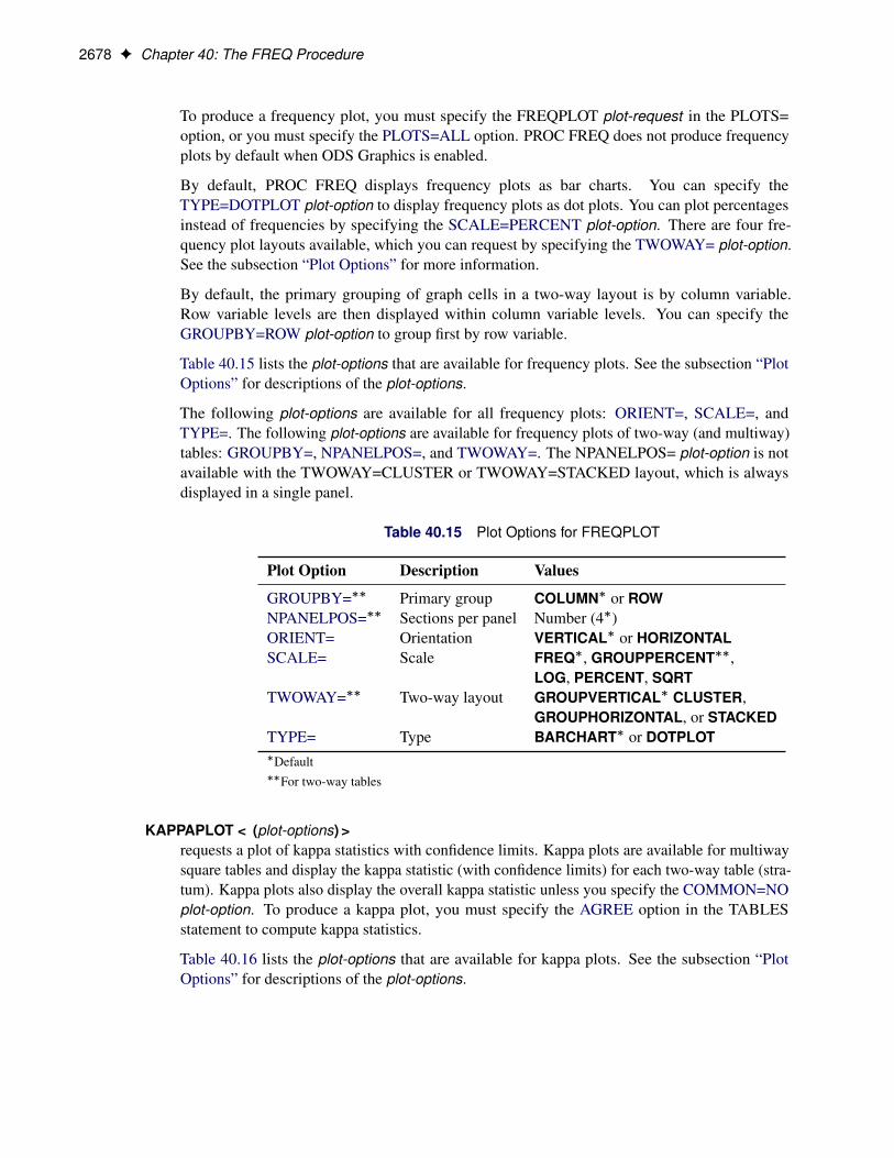
2678 F Chapter 40: The FREQ Procedure
To produce a frequency plot, you must specify the FREQPLOT plot-request in the PLOTS=option, or you must specify the PLOTS=ALL option. PROC FREQ does not produce frequencyplots by default when ODS Graphics is enabled.
By default, PROC FREQ displays frequency plots as bar charts. You can specify theTYPE=DOTPLOT plot-option to display frequency plots as dot plots. You can plot percentagesinstead of frequencies by specifying the SCALE=PERCENT plot-option. There are four fre-quency plot layouts available, which you can request by specifying the TWOWAY= plot-option.See the subsection “Plot Options” for more information.
By default, the primary grouping of graph cells in a two-way layout is by column variable.Row variable levels are then displayed within column variable levels. You can specify theGROUPBY=ROW plot-option to group first by row variable.
Table 40.15 lists the plot-options that are available for frequency plots. See the subsection “PlotOptions” for descriptions of the plot-options.
The following plot-options are available for all frequency plots: ORIENT=, SCALE=, andTYPE=. The following plot-options are available for frequency plots of two-way (and multiway)tables: GROUPBY=, NPANELPOS=, and TWOWAY=. The NPANELPOS= plot-option is notavailable with the TWOWAY=CLUSTER or TWOWAY=STACKED layout, which is alwaysdisplayed in a single panel.
Table 40.15 Plot Options for FREQPLOT
Plot Option Description Values
GROUPBY=�� Primary group COLUMN� or ROWNPANELPOS=�� Sections per panel Number (4�)ORIENT= Orientation VERTICAL� or HORIZONTALSCALE= Scale FREQ�, GROUPPERCENT��,
LOG, PERCENT, SQRTTWOWAY=�� Two-way layout GROUPVERTICAL� CLUSTER,
GROUPHORIZONTAL, or STACKEDTYPE= Type BARCHART� or DOTPLOT�Default��For two-way tables
KAPPAPLOT < (plot-options) >requests a plot of kappa statistics with confidence limits. Kappa plots are available for multiwaysquare tables and display the kappa statistic (with confidence limits) for each two-way table (stra-tum). Kappa plots also display the overall kappa statistic unless you specify the COMMON=NOplot-option. To produce a kappa plot, you must specify the AGREE option in the TABLESstatement to compute kappa statistics.
Table 40.16 lists the plot-options that are available for kappa plots. See the subsection “PlotOptions” for descriptions of the plot-options.

TABLES Statement F 2679
Table 40.16 Plot Options for KAPPAPLOT and WTKAPPAPLOT
Plot Option Description Values
CLDISPLAY= Error bar type SERIF�, SERIFARROW,LINE, LINEARROW, or BAR
COMMON= Overall kappa YES� or NONPANELPOS= Statistics per graphic Number (All�)ORDER= Order of two-way levels ASCENDING or DESCENDINGRANGE= Range to display Values or CLIPSTATS Statistic values None�Default
MOSAICPLOT < (plot-options) >requests a mosaic plot. Mosaic plots are available for two-way and multiway crosstabulationtables; for multiway tables, PROC FREQ provides a mosaic plot for each two-way table (stratum).
To produce a mosaic plot, you must specify the MOSAICPLOT plot-request in the PLOTS=option, or you must specify the PLOTS=ALL option. PROC FREQ does not produce mosaicplots by default when ODS Graphics is enabled.
Mosaic plots display tiles that correspond to the crosstabulation table cells. The areas of the tilesare proportional to the frequencies of the table cells. The column variable is displayed on the Xaxis, and the tile widths are proportional to the relative frequencies of the column variable levels.The row variable is displayed on the Y axis, and the tile heights are proportional to the relativefrequencies of the row levels within column levels. For more information, see Friendly (2000).
By default, the colors of the tiles correspond to the row variable levels. If you specify theCOLORSTAT= plot-option, the tiles are colored according to the values of the Pearson orstandardized residuals.
You can specify the following plot-options:
COLORSTAT < =PEARSONRES | STDRES >colors the mosaic plot tiles according to the values of residuals. If you specify COL-ORSTAT=PEARSONRES, the tiles are colored according to the Pearson residuals of thecorresponding table cells. For more information, see the section “Pearson Chi-SquareTest for Two-Way Tables” on page 2705. If you specify COLORSTAT=STDRES, thetiles are colored according to the standardized residuals of the corresponding table cells.For more information, see the section “Standardized Residuals” on page 2705. You candisplay the Pearson or standardized residuals in the CROSSLIST table by specifying theCROSSLIST(PEARSONRES) or CROSSLIST(STDRES) option, respectively.
SQUAREproduces a square mosaic plot, where the height of the Y axis equals the width of the X axis.In a square mosaic plot, the scale of the relative frequencies is the same on both axes. Bydefault, PROC FREQ produces a rectangular mosaic plot.

2680 F Chapter 40: The FREQ Procedure
NONEsuppresses all plots.
ODDSRATIOPLOT < (plot-options) >requests a plot of odds ratios with confidence limits. Odds ratio plots are available for multiway2 � 2 tables and display the odds ratio (with confidence limits) for each 2 � 2 table (stratum).To produce an odds ratio plot, you must also specify the MEASURES, OR(CL=), or RELRISKoption in the TABLES statement to compute odds ratios.
By default, the odds ratio plot displays asymptotic Wald confidence limits for the odds ratios(CL=WALD). You can specify the CL=EXACT or CL=SCORE plot-option to display exact orscore confidence limits, respectively. To display exact or score confidence limits, you must alsorequest their computation. You can specify the OR option in the EXACT statement to requestexact confidence limits for the odds ratio; you can specify the OR(CL=SCORE) option in theTABLES statement to request score confidence limits for the odds ratio.
By default, the odds ratio plot displays the common odds ratio when the procedure computesthe common value. You can suppress display of the common odds ratio by specifying theCOMMON=NO plot-option. To compute the common odds ratio for a multiway table, you canspecify the CMH option in the TABLES statement. To display the common odds ratio whenthe plot displays exact confidence limits (CL=EXACT), you must request computation of exactconfidence limits for the common odds ratio by specifying the COMOR option in the EXACTstatement. When you specify the CL=SCORE plot-option, the odds ratio plot does not displaythe common odds ratio.
Table 40.17 lists the plot-options that are available for odds ratio plots. See the subsection “PlotOptions” for descriptions of the plot-options.
Table 40.17 Plot Options for ODDSRATIOPLOT, RELRISKPLOT, and RISKDIFFPLOT
Plot Option Description Values
CL= Confidence limit type TypeCLDISPLAY= Error bar type SERIF�, SERIFARROW,
LINE, LINEARROW, or BARCOMMON= Common value YES� or NOCOLUMN=�� Risk column 1� or 2LOGBASE=��� Axis scale 2, E, or 10NPANELPOS= Statistics per graphic Number (All�)ORDER= Order of two-way levels ASCENDING or DESCENDINGRANGE= Range to display Values or CLIPSTATS Statistic values None�Default��Available for RELRISKPLOT and RISKDIFFPLOT���Available for ODDSRATIOPLOT and RELRISKPLOT
RELRISKPLOT < (plot-options) >requests a plot of relative risks with confidence limits. Relative risk plots are available formultiway 2 � 2 tables and display the relative risk (with confidence limits) for each 2 � 2 table

TABLES Statement F 2681
(stratum). To produce a relative risk plot, you must also specify the MEASURES or RELRISKoption in the TABLES statement to compute relative risks.
If you specify the CMH option in the TABLES statement to compute the common relative risk forthe multiway table, by default the plot displays the common relative risk. The COMMON=NOplot-option suppresses display of the common relative risk. If you do not specify the CMH option,the common relative risk is not available to be displayed in the plot.
By default, relative risk plots display asymptotic confidence limits. You can specify theCL=EXACT plot-option to display exact confidence limits for the relative risks. You mustalso request computation of exact confidence limits by specifying the RELRISK option in theEXACT statement. When you specify the CL=EXACT plot-option, the relative risk plot does notdisplay the common relative risk.
Table 40.17 lists the plot-options that are available for relative risk plots. See the subsection “PlotOptions” for descriptions of the plot-options.
RISKDIFFPLOT < (plot-options) >requests a plot of risk (proportion) differences with confidence limits. Risk difference plots areavailable for multiway 2 � 2 tables and display the risk difference (with confidence limits) foreach 2�2 table (stratum). To produce a risk difference plot, you must also specify the RISKDIFFoption in the TABLES statement to compute risk differences.
By default, risk difference plots display asymptotic Wald confidence limits. You can specify theCL=EXACT plot-option to display exact confidence limits for the risk differences. You mustalso request computation of exact confidence limits by specifying the RISKDIFF option in theEXACT statement.
In addition to Wald and exact confidence limits, you can display the following confidence limittypes in a risk difference plot: Agresti-Caffo, Hauck-Anderson, Miettinen-Nurminen (score),and Newcombe. See the descriptions of the CL= plot-option and the RISKDIFF option for moreinformation.
By default or when you specify CL=WALD, the risk difference plot displays the commonrisk difference when PROC FREQ computes the common value. To compute the commonrisk difference for a multiway table, you can specify the RISKDIFF(COMMON) option in theTABLES statement. When you specify other confidence limit types, the risk difference plot doesnot display the common risk difference. You can suppress display of the common risk differenceby specifying the COMMON=NO plot-option.
Table 40.17 lists the plot-options that are available for risk difference plots. See the subsection“Plot Options” for descriptions of the plot-options.
WTKAPPAPLOT < (plot-options) >requests a plot of weighted kappa coefficients with confidence limits. Weighted kappa plots areavailable for multiway square tables and display the weighted kappa coefficient (with confidencelimits) for each two-way table (stratum). Weighted kappa plots also display the overall weightedkappa coefficient unless you specify the COMMON=NO plot-option.
To produce a weighted kappa plot, you must specify the AGREE option in the TABLES statementto compute weighted kappa coefficients, and the table dimension must be greater than 1.
Table 40.16 lists the plot-options that are available for weighted kappa plots. See the subsection“Plot Options” for descriptions of the plot-options.
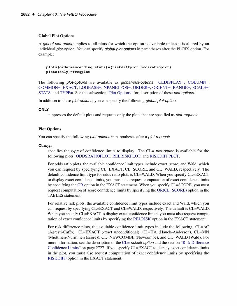
2682 F Chapter 40: The FREQ Procedure
Global Plot Options
A global-plot-option applies to all plots for which the option is available unless it is altered by anindividual plot-option. You can specify global-plot-options in parentheses after the PLOTS option. Forexample:
plots(order=ascending stats)=(riskdiffplot oddsratioplot)plots(only)=freqplot
The following plot-options are available as global-plot-options: CLDISPLAY=, COLUMN=,COMMON=, EXACT, LOGBASE=, NPANELPOS=, ORDER=, ORIENT=, RANGE=, SCALE=,STATS, and TYPE=. See the subsection “Plot Options” for description of these plot-options.
In addition to these plot-options, you can specify the following global-plot-option:
ONLYsuppresses the default plots and requests only the plots that are specified as plot-requests.
Plot Options
You can specify the following plot-options in parentheses after a plot-request:
CL=typespecifies the type of confidence limits to display. The CL= plot-option is available for thefollowing plots: ODDSRATIOPLOT, RELRISKPLOT, and RISKDIFFPLOT.
For odds ratio plots, the available confidence limit types include exact, score, and Wald, whichyou can request by specifying CL=EXACT, CL=SCORE, and CL=WALD, respectively. Thedefault confidence limit type for odds ratio plots is CL=WALD. When you specify CL=EXACTto display exact confidence limits, you must also request computation of exact confidence limitsby specifying the OR option in the EXACT statement. When you specify CL=SCORE, you mustrequest computation of score confidence limits by specifying the OR(CL=SCORE) option in theTABLES statement.
For relative risk plots, the available confidence limit types include exact and Wald, which youcan request by specifying CL=EXACT and CL=WALD, respectively. The default is CL=WALD.When you specify CL=EXACT to display exact confidence limits, you must also request compu-tation of exact confidence limits by specifying the RELRISK option in the EXACT statement.
For risk difference plots, the available confidence limit types include the following: CL=AC(Agresti-Caffo), CL=EXACT (exact unconditional), CL=HA (Hauck-Anderson), CL=MN(Miettinen-Nurminen (score)), CL=NEWCOMBE (Newcombe), and CL=WALD (Wald). Formore information, see the description of the CL= riskdiff-option and the section “Risk DifferenceConfidence Limits” on page 2727. If you specify CL=EXACT to display exact confidence limitsin the plot, you must also request computation of exact confidence limits by specifying theRISKDIFF option in the EXACT statement.

TABLES Statement F 2683
CLDISPLAY=SERIF | SERIFARROW | LINE | LINEARROW | BAR < width >controls the appearance of the confidence limit error bars. This plot-option is available for thefollowing plots: KAPPAPLOT, ODDSRATIOPLOT, RELRISKPLOT, RISKDIFFPLOT, andWTKAPPAPLOT.
The default is CLDISPLAY=SERIF, which displays the confidence limits as lines with serifs.CLDISPLAY=LINE displays the confidence limits as plain lines without serifs. The CLDIS-PLAY=SERIFARROW and CLDISPLAY=LINEARROW plot-options display arrowheads onany error bars that are clipped by the RANGE= plot-option; if an entire error bar is cut from theplot, the plot displays an arrowhead that points toward the statistic.
CLDISPLAY=BAR displays the confidence limits as bars. By default, the width of the barsequals the size of the marker for the estimate. You can control the width of the bars and thesize of the marker by specifying the value of width as a percentage of the distance between bars,0 < width � 1. The bar might disappear when the value of width is very small.
COLUMN=1 | 2specifies the table column to use to compute the risks (proportion) for the relative risk plot(RELRISKPLOT) and the risk difference plot (RISKDIFFPLOT). If you specify COLUMN=1,the plot displays the column 1 relative risks or the column 1 risk differences. Similarly, if youspecify COLUMN=2, the plot displays the column 2 relative risks or risk differences.
For relative risk plots, the default is COLUMN=1. For risk difference plots, the default isCOLUMN=1 if you request computation of both column 1 and column 2 risk differences byspecifying the RISKDIFF option. If you request computation of only the column 1 (or column2) risk differences by specifying the RISKDIFF(COLUMN=1) (or RISKDIFF(COLUMN=2))option, by default the risk difference plot displays the risk differences for the column that youspecify.
COMMON=YES | NOcontrols the display of the common (overall) statistic in plots that display stratum (two-way table)statistics for a multiway table. The COMMON= plot-option is available for the following plots:KAPPAPLOT, ODDSRATIOPLOT, RELRISKPLOT, RISKDIFFPLOT, and WTKAPPAPLOT.
By default, COMMON=YES and plots display the common value when PROC FREQ computesit. When you specify the AGREE option in the TABLES statement for a multiway table, PROCFREQ computes the common simple and weighted kappa coefficients, which can be displayedin the simple and weighted kappa plots, respectively. When you specify the MEASURES orRELRISK option in the TABLES statement, PROC FREQ computes only stratum-level oddsratios and relative risks; to compute common odds ratios and relative risks, you must also specifythe CMH option in the TABLES statement. To compute the common risk difference, you mustspecify the RISKDIFF(COMMON) option. For more information, see the descriptions of theplot-requests.
EXACTrequests display of exact confidence limits instead of asymptotic confidence limits. TheEXACT plot-option is available for the odds ratio plot (ODDSRATIOPLOT), relative risk plot(RELRISKPLOT), and risk difference plot (RISKDIFFPLOT). The EXACT plot-option is equiv-alent to the CL=EXACT plot-option.
When you specify the EXACT plot-option, you must also request computation of exact confidencelimits by specifying the appropriate statistic-option in the EXACT statement.

2684 F Chapter 40: The FREQ Procedure
GROUPBY=COLUMN | ROWspecifies the primary grouping for two-way frequency plots, which you can request by specifyingthe FREQPLOT plot=request . The default is GROUPBY=COLUMN, which groups graph cellsfirst by column variable and displays row variable levels within column variable levels. You canspecify GROUPBY=ROW to group first by row variable. In two-way and multiway table requests,the column variable is the last variable specified and forms the columns of the crosstabulationtable. The row variable is the next-to-last variable specified and forms the rows of the table.
By default for a bar chart that is displayed in the TWOWAY=STACKED layout, bars correspondto the column variable levels, and row levels are displayed (stacked) within each column bar.By default for a bar chart that is displayed in the TWOWAY=CLUSTER layout, bars are firstgrouped by column variable levels, and row levels are displayed as adjacent bars within eachcolumn-level group. You can reverse the default row and column variable grouping by specifyingGROUPBY=ROW.
LOGBASE=2 | E | 10applies to the odds ratio plot (ODDSRATIOPLOT) and the relative risk plot (RELRISKPLOT).This plot-option displays the odds ratio or relative risk axis on the log scale that you specify.
LEGEND=YES | NOapplies to the agreement plot (AGREEPLOT). LEGEND=NO suppresses the legend that identifiesthe areas of exact and partial agreement. The default is LEGEND=YES.
NOSTATapplies to the deviation plot (DEVIATIONPLOT). NOSTAT suppresses the chi-square p-valuethat deviation plot displays by default.
NPANELPOS=ndivides the plot into multiple panels that display at most jnj statistics or sections.
If n is positive, the number of statistics or sections per panel is balanced; if n is negative, thenumber of statistics per panel is not balanced. For example, suppose you want to display 21 oddsratios. NPANELPOS=20 displays two panels, the first with 11 odds ratios and the second with10 odds ratios; NPANELPOS=–20 displays 20 odds ratios in the first panel but only 1 odds ratioin the second panel. This plot-option is available for all plots except mosaic plots and one-wayweighted frequency plots.
For two-way frequency plots (FREQPLOT), NPANELPOS=n requests that panels display at mostjnj sections, where sections correspond to row or column variable levels, depending on the typeof plot and the grouping. By default, n=4 and each panel includes at most four sections. Thisplot-option applies to two-way plots that are displayed in the TWOWAY=GROUPVERTICAL orTWOWAY=GROUPHORIZONTAL layout. The NPANELPOS= plot-option does not apply tothe TWOWAY=CLUSTER and TWOWAY=STACKED layouts, which are always displayed in asingle panel.
For plots that display statistics along with confidence limits, NPANELPOS=n requests thatpanels display at most jnj statistics. By default, n=0 and all statistics are displayed in a singlepanel. This plot-option applies to the following plots: KAPPAPLOT, ORPLOT, RELRISKPLOT,RISKDIFFPLOT, and WTKAPPAPLOT.

TABLES Statement F 2685
ORDER=ASCENDING | DESCENDINGdisplays the two-way table (strata) statistics in order of the statistic value. If you specifyORDER=ASCENDING or ORDER=DESCENDING, the plot displays the statistics in ascendingor descending order, respectively. By default, the order of the statistics in the plot matches theorder that the two-way table strata appear in the multiway table display.
This plot-option applies to the following plots: KAPPAPLOT, ODDSRATIOPLOT, REL-RISKPLOT, RISKDIFFPLOT, and WTKAPPAPLOT.
ORIENT=HORIZONTAL | VERTICALcontrols the orientation of the plot. The ORIENT= plot-option applies to the following plots:CUMFREQPLOT, DEVIATIONPLOT, and FREQPLOT.
ORIENT=HORIZONTAL places the variable levels on the Y axis and the frequencies, percent-ages, or statistic values on the X axis. ORIENT=VERTICAL places the variable levels on the Xaxis. The default orientation is ORIENT=VERTICAL for bar charts (TYPE=BARCHART) andORIENT=HORIZONTAL for dot plots (TYPE=DOTPLOT).
PARTIAL=YES | NOcontrols the display of partial agreement in the agreement plot (AGREEPLOT). PARTIAL=NOsuppresses the display of partial agreement. When you specify PARTIAL=NO, the agreementplot displays only exact agreement. Exact agreement includes the diagonal cells of the squaretable, where the row and column variable levels are the same. Partial agreement includes theadjacent off-diagonal table cells, where the row and column values are within one level of exactagreement. The default is PARTIAL=YES.
RANGE=( < min > < , max > )| CLIPspecifies the range of values to display. If you specify RANGE=CLIP, the confidence limitsare clipped and the display range is determined by the minimum and maximum values of thestatistics. By default, the display range includes all confidence limits.
This plot-option is available for the following plots: KAPPAPLOT, ODDSRATIOPLOT, REL-RISKPLOT, RISKDIFFPLOT, and WTKAPPAPLOT.
SCALE=FREQ | GROUPPERCENT | LOG | PERCENT | SQRTspecifies the scale of the frequencies to display. This plot-option is available for frequency plots(FREQPLOT) and cumulative frequency plots (CUMFREQPLOT).
The default is SCALE=FREQ, which displays unscaled frequencies. SCALE=PERCENT displayspercentages (relative frequencies) of the total frequency. SCALE=LOG displays log (base 10)frequencies. SCALE=SQRT displays square roots of the frequencies, producing a plot known asa rootogram.
SCALE=GROUPPERCENT is available for two-way frequency plots. This option displays therow or column percentages instead of the overall percentages (of the table frequency). By default(or when you specify the GROUPBY=COLUMN plot-option), SCALE=GROUPPERCENTdisplays the column percentages. If you specify the GROUPBY=ROW plot-option, the primarygrouping of graph cells is by row variable level and the plot displays row percentages. For moreinformation, see the description of the GROUPBY= plot-option.

2686 F Chapter 40: The FREQ Procedure
SHOWSCALE=YES | NOcontrols the display of the cumulative frequency scale on the right side of the agreement plot(AGREEPLOT). SHOWSCALE=NO suppresses the display of the scale. The default is SHOWS-CALE=YES.
STATSdisplays statistic values in the plot. For the following plots, the STATS plot-option dis-plays the statistics and their confidence limits on the right side of the plot: KAPPAPLOT,ODDSRATIOPLOT, RELRISKPLOT, RISKDIFFPLOT, and WTKAPPAPLOT.
For the agreement plot (AGREEPLOT), STATS displays the values of the kappa statistic, theweighted kappa statistic, and the Bn measure (Bangdiwala and Bryan 1987).
If you do not request the STATS plot-option, these plots do not display the statistic values.
TWOWAY=CLUSTER | GROUPHORIZONTAL | GROUPVERTICAL | STACKEDspecifies the layout for two-way frequency plots.
All TWOWAY= layouts are available for bar charts (TYPE=BARCHART). All TWOWAY=layouts except TWOWAY=CLUSTER are available for dot plots (TYPE=DOTPLOT). TheORIENT= and GROUPBY= plot-options are available for all TWOWAY= layouts.
The default two-way layout is TWOWAY=GROUPVERTICAL, which produces a groupedplot that has a vertical common baseline. By default for bar charts (TYPE=BARCHART,ORIENT=VERTICAL), the X axis displays column variable levels, and the Y axis displaysfrequencies. The plot includes a vertical (Y-axis) block for each row variable level. The relativepositions of the graph cells in this plot layout are the same as the relative positions of the tablecells in the crosstabulation table. You can reverse the default row and column grouping byspecifying the GROUPBY=ROW plot-option.
The TWOWAY=GROUPHORIZONTAL layout produces a grouped plot that has a horizontalcommon baseline. By default (GROUPBY=COLUMN), the plot displays a block on the X axisfor each column variable level. Within each column-level block, the plot displays row variablelevels.
The TWOWAY=STACKED layout produces stacked displays of frequencies. By default(GROUPBY=COLUMN) in a stacked bar chart, the bars correspond to column variable levels,and row levels are stacked within each column level. By default in a stacked dot plot, thedotted lines correspond to column levels, and cell frequencies are plotted as data dots on thecorresponding column line. The dot color identifies the row level.
The TWOWAY=CLUSTER layout, which is available only for bar charts, displays groups ofadjacent bars. By default, the primary grouping is by column variable level, and row levels aredisplayed within each column level.
You can reverse the default row and column grouping in any layout by specifying theGROUPBY=ROW plot-option. The default is GROUPBY=COLUMN, which groups first bycolumn variable.
TYPE=BARCHART | DOTPLOTspecifies the plot type (format) of the frequency (FREQPLOT), cumulative frequency(CUMFREQPLOT), and deviation plots (DEVIATIONPLOT). TYPE=BARCHART produces abar chart and TYPE=DOTPLOT produces a dot plot. The default is TYPE=BARCHART.

TABLES Statement F 2687
PRINTKWTSdisplays the agreement weights that PROC FREQ uses to compute the weighted kappa coefficient.Agreement weights reflect the relative agreement between pairs of variable levels. By default, PROCFREQ uses the Cicchetti-Allison form of agreement weights. If you specify the AGREE(WT=FC)option, the procedure uses the Fleiss-Cohen form of agreement weights. For more information, see thesection “Weighted Kappa Coefficient” on page 2745.
This option has no effect unless you also specify the AGREE option to compute the weighted kappacoefficient. The PRINTKWTS option is equivalent to the AGREE(PRINTKWTS) option.
RELRISK
ORrequests relative risk measures and their asymptotic Wald confidence limits for 2 � 2 tables. Thesemeasures include the odds ratio, the column 1 relative risk, and the column 2 relative risk. PROCFREQ displays the statistics and confidence limits in the “Odds Ratio and Relative Risks” table. Formore information, see the section “Odds Ratio and Relative Risks for 2 x 2 Tables” on page 2737.
You can request exact confidence limits for the odds ratio by specifying the OR option in the EXACTstatement. You can request exact unconditional confidence limits for the relative risks by specifying theRELRISK option in the EXACT statement. For more information, see the sections “Exact ConfidenceLimits for the Odds Ratio” on page 2738 and “Exact Unconditional Confidence Limits for the RelativeRisk” on page 2739.
You can request score confidence limits for the odds ratio by specifying the OR(CL=) option. Thisoption produces the “Confidence Limits for the Odds Ratio” table, which can also display Wald andexact confidence limits. For more information, see the section “Score Confidence Limits for the OddsRatio” on page 2738.
You can also obtain the relative risk measures by specifying the MEASURES option, which producesother measures of association in addition to the relative risks.
RISKDIFF < (riskdiff-options) >requests risks (binomial proportions) and risk differences for 2 � 2 tables. When you specify theRISKDIFF option, PROC FREQ provides the row 1 risk, row 2 risk, total (overall) risk, and riskdifference (row 1 – row 2), together with their asymptotic standard errors and Wald confidence limits.PROC FREQ also provides exact (Clopper-Pearson) confidence limits for the row 1, row 2, and totalrisks by default. You can request exact unconditional confidence limits for the risk difference byspecifying the RISKDIFF option in the EXACT statement. For more information, see the section“Risks and Risk Differences” on page 2725. PROC FREQ displays these results in the column 1 andcolumn 2 “Risk Estimates” tables.
You can specify riskdiff-options in parentheses after the RISKDIFF option to request tests and additionalconfidence limits for the risk difference, as well as estimates of the common risk difference for multiway2 � 2 tables. Table 40.18 summarizes the riskdiff-options.
The CL= riskdiff-option requests confidence limits for the risk difference. Available confidence limittypes include Agresti-Caffo, exact unconditional, Hauck-Anderson, Miettinen-Nurminen (score),Newcombe, and Wald. Continuity-corrected Newcombe and Wald confidence limits are also available.You can request more than one type of confidence limits in the same analysis. PROC FREQ displaysthe confidence limits in the “Confidence Limits for the Proportion (Risk) Difference” table.

2688 F Chapter 40: The FREQ Procedure
The CL=EXACT riskdiff-option displays exact unconditional confidence limits in the “Proportion (Risk)Difference Confidence Limits” table. When you use CL=EXACT, you must also request computationof the exact confidence limits by specifying the RISKDIFF option in the EXACT statement.
The EQUIV, NONINF, and SUP riskdiff-options request tests of equivalence, noninferiority, andsuperiority, respectively, for the risk difference. Available test methods include Farrington-Manning(score), Hauck-Anderson, and Newcombe (hybrid-score), in addition to the Wald test.
As part of the noninferiority, superiority, and equivalence analyses, PROC FREQ provides null-basedequivalence limits that have a confidence coefficient of 100.1 � 2˛/% (Schuirmann 1999). TheALPHA= option determines the confidence level, and the default of ALPHA=0.05 produces 90%equivalence limits. See the sections “Noninferiority Tests” on page 2731 and “Equivalence Tests” onpage 2733 for details.
Table 40.18 RISKDIFF (Proportion Difference) Options
Option Description
COLUMN=1 | 2 Specifies the risk columnCOMMON Requests common risk differenceCORRECT Requests continuity correctionNORISKS Suppresses default risk tables
Request Confidence LimitsCL=AC Requests Agresti-Caffo confidence limitsCL=EXACT Displays exact confidence limitsCL=HA Requests Hauck-Anderson confidence limitsCL=MN | SCORE Requests Miettinen-Nurminen confidence limitsCL=NEWCOMBE Requests Newcombe confidence limitsCL=WALD Requests Wald confidence limits
Request TestsEQUAL Requests an equality testEQUIV | EQUIVALENCE Requests an equivalence testNONINF | NONINFERIORITY Requests a noninferiority testSUP | SUPERIORITY Requests a superiority testMARGIN= Specifies the test marginMETHOD= Specifies the test methodVAR=SAMPLE | NULL Specifies the test variance
You can specify the following riskdiff-options in parentheses after the RISKDIFF option:
CL=type | (types)requests confidence limits for the risk difference. You can specify one or more types of confidencelimits. When you specify only one type, you can omit the parentheses around the request. PROCFREQ displays the confidence limits in the “Proportion (Risk) Difference Confidence Limits”table.
The ALPHA= option determines the confidence level, and the default of ALPHA=0.05 produces95% confidence limits for the risk difference. This differs from the test-based confidence limitsthat are provided with the equivalence, noninferiority, and superiority tests (EQUIV, NONINF,and SUP), which have a confidence coefficient of 100.1 � 2˛/% (Schuirmann 1999).
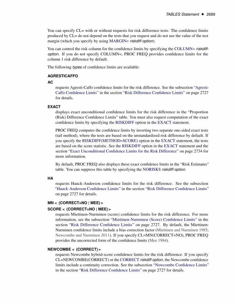
TABLES Statement F 2689
You can specify CL= with or without requests for risk difference tests. The confidence limitsproduced by CL= do not depend on the tests that you request and do not use the value of the testmargin (which you specify by using MARGIN= riskdiff-option).
You can control the risk column for the confidence limits by specifying the COLUMN= riskdiff-option. If you do not specify COLUMN=, PROC FREQ provides confidence limits for thecolumn 1 risk difference by default.
The following types of confidence limits are available:
AGRESTICAFFO
ACrequests Agresti-Caffo confidence limits for the risk difference. See the subsection “Agresti-Caffo Confidence Limits” in the section “Risk Difference Confidence Limits” on page 2727for details.
EXACTdisplays exact unconditional confidence limits for the risk difference in the “Proportion(Risk) Difference Confidence Limits” table. You must also request computation of the exactconfidence limits by specifying the RISKDIFF option in the EXACT statement.
PROC FREQ computes the confidence limits by inverting two separate one-sided exact tests(tail method), where the tests are based on the unstandardized risk difference by default. Ifyou specify the RISKDIFF(METHOD=SCORE) option in the EXACT statement, the testsare based on the score statistic. See the RISKDIFF option in the EXACT statement and thesection “Exact Unconditional Confidence Limits for the Risk Difference” on page 2734 formore information.
By default, PROC FREQ also displays these exact confidence limits in the “Risk Estimates”table. You can suppress this table by specifying the NORISKS riskdiff-option.
HArequests Hauck-Anderson confidence limits for the risk difference. See the subsection“Hauck-Anderson Confidence Limits” in the section “Risk Difference Confidence Limits”on page 2727 for details.
MN < (CORRECT=NO | MEE) >
SCORE < (CORRECT=NO | MEE) >requests Miettinen-Nurminen (score) confidence limits for the risk difference. For moreinformation, see the subsection “Miettinen-Nurminen (Score) Confidence Limits” in thesection “Risk Difference Confidence Limits” on page 2727. By default, the Miettinen-Nurminen confidence limits include a bias correction factor (Miettinen and Nurminen 1985;Newcombe and Nurminen 2011). If you specify CL=MN(CORRECT=NO), PROC FREQprovides the uncorrected form of the confidence limits (Mee 1984).
NEWCOMBE < (CORRECT) >requests Newcombe hybrid-score confidence limits for the risk difference. If you specifyCL=NEWCOMBE(CORRECT) or the CORRECT riskdiff-option, the Newcombe confidencelimits include a continuity correction. See the subsection “Newcombe Confidence Limits”in the section “Risk Difference Confidence Limits” on page 2727 for details.
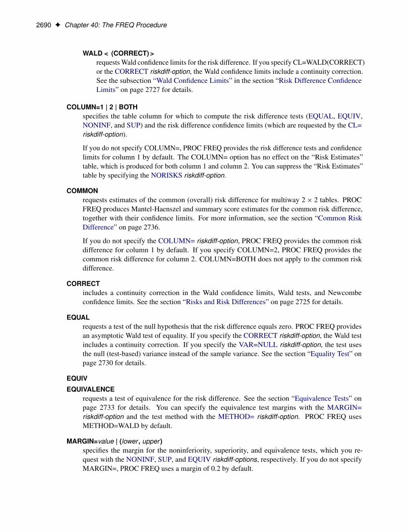
2690 F Chapter 40: The FREQ Procedure
WALD < (CORRECT) >requests Wald confidence limits for the risk difference. If you specify CL=WALD(CORRECT)or the CORRECT riskdiff-option, the Wald confidence limits include a continuity correction.See the subsection “Wald Confidence Limits” in the section “Risk Difference ConfidenceLimits” on page 2727 for details.
COLUMN=1 | 2 | BOTHspecifies the table column for which to compute the risk difference tests (EQUAL, EQUIV,NONINF, and SUP) and the risk difference confidence limits (which are requested by the CL=riskdiff-option).
If you do not specify COLUMN=, PROC FREQ provides the risk difference tests and confidencelimits for column 1 by default. The COLUMN= option has no effect on the “Risk Estimates”table, which is produced for both column 1 and column 2. You can suppress the “Risk Estimates”table by specifying the NORISKS riskdiff-option.
COMMONrequests estimates of the common (overall) risk difference for multiway 2 � 2 tables. PROCFREQ produces Mantel-Haenszel and summary score estimates for the common risk difference,together with their confidence limits. For more information, see the section “Common RiskDifference” on page 2736.
If you do not specify the COLUMN= riskdiff-option, PROC FREQ provides the common riskdifference for column 1 by default. If you specify COLUMN=2, PROC FREQ provides thecommon risk difference for column 2. COLUMN=BOTH does not apply to the common riskdifference.
CORRECTincludes a continuity correction in the Wald confidence limits, Wald tests, and Newcombeconfidence limits. See the section “Risks and Risk Differences” on page 2725 for details.
EQUALrequests a test of the null hypothesis that the risk difference equals zero. PROC FREQ providesan asymptotic Wald test of equality. If you specify the CORRECT riskdiff-option, the Wald testincludes a continuity correction. If you specify the VAR=NULL riskdiff-option, the test usesthe null (test-based) variance instead of the sample variance. See the section “Equality Test” onpage 2730 for details.
EQUIV
EQUIVALENCErequests a test of equivalence for the risk difference. See the section “Equivalence Tests” onpage 2733 for details. You can specify the equivalence test margins with the MARGIN=riskdiff-option and the test method with the METHOD= riskdiff-option. PROC FREQ usesMETHOD=WALD by default.
MARGIN=value | (lower , upper )specifies the margin for the noninferiority, superiority, and equivalence tests, which you re-quest with the NONINF, SUP, and EQUIV riskdiff-options, respectively. If you do not specifyMARGIN=, PROC FREQ uses a margin of 0.2 by default.

TABLES Statement F 2691
For noninferiority and superiority tests, specify a single value for MARGIN=. The MARGIN=value must be a positive number. You can specify value as a number between 0 and 1. Or youcan specify value in percentage form as a number between 1 and 100, and PROC FREQ convertsthat number to a proportion. The procedure treats the value 1 as 1%.
For an equivalence test, you can specify a single MARGIN= value, or you can specify both lowerand upper values. If you specify a single MARGIN= value, it must be a positive number, asdescribed previously. If you specify a single MARGIN= value for an equivalence test, PROCFREQ uses –value as the lower margin and value as the upper margin for the test. If you specifyboth lower and upper values for an equivalence test, you can specify them in proportion form asnumbers between –1 or 1. Or you can specify them in percentage form as numbers between –100and 100, and PROC FREQ converts the numbers to proportions. The value of lower must be lessthan the value of upper .
METHOD=methodspecifies the method for the noninferiority, superiority, and equivalence analyses, which yourequest with the NONINF, SUP, and EQUIV riskdiff-options, respectively. If you do not specifythe METHOD= riskdiff-option, PROC FREQ uses METHOD=WALD by default.
The following methods are available:
FMSCORE
requests Farrington-Manning (score) tests and equivalence limits for the equivalence, nonin-feriority, and superiority analyses. See the subsection “Farrington-Manning (Score) Test” inthe section “Noninferiority Tests” on page 2731 for details.
HArequests Hauck-Anderson tests and confidence limits for the equivalence, noninferiority, andsuperiority analyses. See the subsection “Hauck-Anderson Test” in the section “Noninferior-ity Tests” on page 2731 for details.
NEWCOMBErequests Newcombe (hybrid-score) confidence limits for the equivalence, noninferiority, andsuperiority analyses. If you specify the CORRECT riskdiff-option, the Newcombe confi-dence limits include a continuity correction. See the subsection “Newcombe NoninferiorityAnalysis” in the section “Noninferiority Tests” on page 2731 for details.
WALDrequests Wald tests and confidence limits for the equivalence, noninferiority, and superiorityanalyses. If you specify the CORRECT riskdiff-option, the Wald confidence limits include acontinuity correction. If you specify the VAR=NULL riskdiff-option, the tests and confidencelimits use the null (test-based) variance instead of the sample variance. See the subsection“Wald Test” in the section “Noninferiority Tests” on page 2731 for details.
NONINFNONINFERIORITY
requests a test of noninferiority for the risk difference. See the section “Noninferiority Tests” onpage 2731 for details. You can specify the test margin with the MARGIN= riskdiff-option andthe test method with the METHOD= riskdiff-option. PROC FREQ uses METHOD=WALD bydefault.

2692 F Chapter 40: The FREQ Procedure
NORISKSsuppresses display of the “Risk Estimates” tables, which the RISKDIFF option produces bydefault for column 1 and column 2. The “Risk Estimates” tables contain the risks and riskdifferences, together with their asymptotic standard errors, Wald confidence limits, and exactconfidence limits.
SUP
SUPERIORITYrequests a test of superiority for the binomial proportion. See the section “Superiority Test” onpage 2733 for details. You can specify the test margin with the MARGIN= riskdiff-option andthe test method with the METHOD= riskdiff-option. PROC FREQ uses METHOD=WALD bydefault.
VAR=SAMPLE | NULLspecifies the type of variance estimate to use in the Wald tests of noninferiority, superiority,equivalence, and equality. The default is VAR=SAMPLE, which uses the sample variance.VAR=NULL uses a test-based variance that is computed by using the null hypothesis riskdifference value. See the sections “Equality Test” on page 2730 and “Noninferiority Tests” onpage 2731 for details.
SCORES=typespecifies the type of row and column scores that PROC FREQ uses to compute the following statistics:Mantel-Haenszel chi-square, Pearson correlation, Cochran-Armitage test for trend, weighted kappacoefficient, and Cochran-Mantel-Haenszel statistics. The value of type can be one of the following:
• MODRIDIT
• RANK
• RIDIT
• TABLE
See the section “Scores” on page 2703 for descriptions of these score types.
If you do not specify the SCORES= option, PROC FREQ uses SCORES=TABLE by default. Forcharacter variables, the row and column TABLE scores are the row and column numbers. That is,the TABLE score is 1 for row 1, 2 for row 2, and so on. For numeric variables, the row and columnTABLE scores equal the variable values. See the section “Scores” on page 2703 for details. UsingMODRIDIT, RANK, or RIDIT scores yields nonparametric analyses.
You can use the SCOROUT option to display the row and column scores.
SCOROUTdisplays the row and column scores that PROC FREQ uses to compute score-based tests and statistics.You can specify the score type with the SCORES= option. See the section “Scores” on page 2703 fordetails.
The scores are computed and displayed only when PROC FREQ computes statistics for two-way tables.You can use ODS to store the scores in an output data set. See the section “ODS Table Names” onpage 2773 for more information.
TEST Statement F 2693
SPARSEreports all possible combinations of the variable values for an n-way table when n > 1, even if acombination does not occur in the data. The SPARSE option applies only to crosstabulation tablesdisplayed in LIST format and to the OUT= output data set. If you do not use the LIST or OUT= option,the SPARSE option has no effect.
When you specify the SPARSE and LIST options, PROC FREQ displays all combinations of variablevalues in the table listing, including those with a frequency count of zero. By default, without theSPARSE option, PROC FREQ does not display zero-frequency levels in LIST output. When you usethe SPARSE and OUT= options, PROC FREQ includes empty crosstabulation table cells in the outputdata set. By default, PROC FREQ does not include zero-frequency table cells in the output data set.
See the section “Missing Values” on page 2699 for more information.
TOTPCTdisplays the percentage of the total multiway table frequency in crosstabulation tables for n-waytables, where n > 2. By default, PROC FREQ displays the percentage of the individual two-way tablefrequency but does not display the percentage of the total frequency for multiway crosstabulationtables. See the section “Two-Way and Multiway Tables” on page 2767 for more information.
The percentage of total multiway table frequency is displayed by default when you specify the LISToption. It is also provided by default in the PERCENT variable in the OUT= output data set.
TRENDrequests the Cochran-Armitage test for trend. The table must be 2 � C or R � 2 to compute the trendtest. See the section “Cochran-Armitage Test for Trend” on page 2740 for details. To request exactp-values for the trend test, specify the TREND option in the EXACT statement. See the section “ExactStatistics” on page 2757 for more information.
TEST StatementTEST test-options ;
The TEST statement requests asymptotic tests for measures of association and measures of agreement. Thetest-options identify which tests to compute. Table 40.19 lists the available test-options, together with theircorresponding TABLES statement options. Descriptions of the test-options follow the table in alphabeticalorder.
For each measure of association or agreement that you request in the TEST statement, PROC FREQ providesan asymptotic test that the measure equals zero. The procedure displays the asymptotic standard errorunder the null hypothesis, the test statistic, and the one-sided and two-sided p-values. Additionally, PROCFREQ reports the confidence limits for the measure. The ALPHA= option in the TABLES statementdetermines the confidence level, which by default equals 0.05 and provides 95% confidence limits. See thesections “Asymptotic Tests” on page 2710 and “Confidence Limits” on page 2710 for details. Also see thesections “Measures of Association” on page 2709 and “Tests and Measures of Agreement” on page 2743 forinformation about the individual measures.
You can also request exact tests for selected measures of association and agreement by using the EXACTstatement. See the section “Exact Statistics” on page 2757 for more information.

2694 F Chapter 40: The FREQ Procedure
Using the TEST Statement with the TABLES StatementYou must use a TABLES statement with the TEST statement. If you use only one TABLES statement, youdo not need to specify the same options in both the TABLES and TEST statements; when you specify anoption in the TEST statement, PROC FREQ automatically invokes the corresponding TABLES statementoption. However, when you use the TEST statement with multiple TABLES statements, you must specifyoptions in the TABLES statements to request statistics. PROC FREQ then provides asymptotic tests for thosestatistics that you also specify in the TEST statement.
Table 40.19 TEST Statement Options
Test Option Asymptotic Tests Required TABLESStatement Option
AGREE Simple and weighted kappa coefficients AGREEGAMMA Gamma ALL or MEASURESKAPPA Simple kappa coefficient AGREEKENTB | TAUB Kendall’s tau-b ALL or MEASURESMEASURES Gamma, Kendall’s tau-b, Stuart’s tau-c, ALL or MEASURES
Somers’ D.C jR/, Somers’ D.RjC/,Pearson and Spearman correlations
PCORR Pearson correlation coefficient ALL or MEASURESPLCORR Polychoric correlation PLCORRSCORR Spearman correlation coefficient ALL or MEASURESSMDCR Somers’ D.C jR/ ALL or MEASURESSMDRC Somers’ D.RjC/ ALL or MEASURESSTUTC | TAUC Stuart’s tau-c ALL or MEASURESWTKAP | WTKAPPA Weighted kappa coefficient AGREE
You can specify the following test-options in the TEST statement.
AGREErequests asymptotic tests for the simple kappa coefficient and the weighted kappa coefficient. See thesections “Simple Kappa Coefficient” on page 2744 and “Weighted Kappa Coefficient” on page 2745for details.
The AGREE option in the TABLES statement provides estimates, standard errors, and confidencelimits for kappa coefficients. You can request exact tests for kappa coefficients by using the EXACTstatement.
Kappa coefficients are defined only for square tables, where the number of rows equals the numberof columns. Kappa coefficients are not computed for tables that are not square. For 2 � 2 tables, theweighted kappa coefficient is identical to the simple kappa coefficient, and PROC FREQ presents onlythe simple kappa coefficient.
GAMMArequests an asymptotic test for the gamma statistic. See the section “Gamma” on page 2711 for details.The MEASURES option in the TABLES statement provides the gamma statistic and its asymptoticstandard error.
TEST Statement F 2695
KAPPArequests an asymptotic test for the simple kappa coefficient. See the section “Simple Kappa Coefficient”on page 2744 for details.
The AGREE option in the TABLES statement provides the kappa statistic, its standard error, and itsconfidence limits. You can request an exact test for the simple kappa coefficient by specifying theKAPPA option in the EXACT statement.
Kappa coefficients are defined only for square tables, where the number of rows equals the number ofcolumns. PROC FREQ does not compute kappa coefficients for tables that are not square.
KENTB
TAUBrequests an asymptotic test for Kendall’s tau-b. See the section “Kendall’s Tau-b” on page 2711 fordetails.
The MEASURES option in the TABLES statement provides Kendall’s tau-b and its standard error. Youcan request an exact test for Kendall’s tau-b by specifying the KENTB option in the EXACT statement.
MEASURESrequests asymptotic tests for the following measures of association: gamma, Kendall’s tau-b, Pearsoncorrelation coefficient, Somers’ D.C jR/, Somers’ D.RjC/, Spearman correlation coefficient, andStuart’s tau-c. See the section “Measures of Association” on page 2709 for details.
The MEASURES option in the TABLES statement provides measures of association and their asymp-totic standard errors. You can request exact tests for selected measures by using the EXACT statement.
PCORRrequests an asymptotic test for the Pearson correlation coefficient. See the section “Pearson CorrelationCoefficient” on page 2713 for details.
The MEASURES option in the TABLES statement provides the Pearson correlation and its standarderror. You can request an exact test for the Pearson correlation by specifying the PCORR option in theEXACT statement.
PLCORRrequests Wald and likelihood ratio tests for the polychoric correlation coefficient. See the section“Polychoric Correlation” on page 2715 for details.
The PLCORR option in the TABLES statement provides the polychoric correlation and its standarderror.
SCORRrequests an asymptotic test for the Spearman correlation coefficient. See the section “Spearman RankCorrelation Coefficient” on page 2714 for details.
The MEASURES option in the TABLES statement provides the Spearman correlation and its standarderror. You can request an exact test for the Spearman correlation by specifying the SCORR option inthe EXACT statement.
2696 F Chapter 40: The FREQ Procedure
SMDCRrequests an asymptotic test for Somers’ D.C jR/. See the section “Somers’ D” on page 2712 fordetails.
The MEASURES option in the TABLES statement provides Somers’ D.C jR/ and its standard error.You can request an exact test for Somers’ D.C jR/ by specifying the SMDCR option in the EXACTstatement.
SMDRCrequests an asymptotic test for Somers’ D.RjC/. See the section “Somers’ D” on page 2712 fordetails.
The MEASURES option in the TABLES statement provides Somers’ D.RjC/ and its standard error.You can request an exact test for Somers’ D.RjC/ by specifying the SMDRC option in the EXACTstatement.
STUTC
TAUCrequests an asymptotic test for Stuart’s tau-c. See the section “Stuart’s Tau-c” on page 2712 for details.
The MEASURES option in the TABLES statement provides Stuart’s tau-c and its standard error. Youcan request an exact test for Stuart’s tau-c by specifying the STUTC option in the EXACT statement.
WTKAP
WTKAPPArequests an asymptotic test for the weighted kappa coefficient. See the section “Weighted KappaCoefficient” on page 2745 for details.
The AGREE option in the TABLES statement provides the weighted kappa coefficient, its standarderror, and confidence limits. You can request an exact test for the weighted kappa by specifying theWTKAP option in the EXACT statement.
Kappa coefficients are defined only for square tables, where the number of rows equals the number ofcolumns. PROC FREQ does not compute kappa coefficients for tables that are not square. For 2 � 2tables, the weighted kappa coefficient is identical to the simple kappa coefficient, and PROC FREQpresents only the simple kappa coefficient.
WEIGHT StatementWEIGHT variable < / option > ;
The WEIGHT statement names a numeric variable that provides a weight for each observation in the inputdata set. The WEIGHT statement is most commonly used to input cell count data. See the section “InputtingFrequency Counts” on page 2697 for more information. If you use a WEIGHT statement, PROC FREQassumes that an observation represents n observations, where n is the value of variable. The value of theWEIGHT variable is not required to be an integer.
If the value of the WEIGHT variable is missing, PROC FREQ does not use that observation in the analysis.If the value of the WEIGHT variable is zero, PROC FREQ ignores the observation unless you specify theZEROS option, which includes observations with zero weights. If you do not specify a WEIGHT statement,

Details: FREQ Procedure F 2697
PROC FREQ assigns a weight of one to each observation. The sum of the WEIGHT variable values representsthe total number of observations.
If any value of the WEIGHT variable is negative, PROC FREQ displays the frequencies computed fromthe weighted values but does not compute percentages and statistics. If you create an output data set byusing the OUT= option in the TABLES statement, PROC FREQ assigns missing values to the PERCENTvariable. PROC FREQ also assigns missing values to the variables that the OUTEXPECT and OUTPCToptions provide. If any value of the WEIGHT variable is negative, you cannot create an output data set byusing the OUTPUT statement because statistics are not computed when there are negative weights.
You can specify the following option in the WEIGHT statement:
ZEROSincludes observations with zero weight values. By default, PROC FREQ ignores observations withzero weights.
If you specify the ZEROS option, frequency and and crosstabulation tables display any levels cor-responding to observations with zero weights. Without the ZEROS option, PROC FREQ does notprocess observations with zero weights, and so does not display levels that contain only observationswith zero weights.
With the ZEROS option, PROC FREQ includes levels with zero weights in the chi-square goodness-of-fit test for one-way tables. Also, PROC FREQ includes any levels with zero weights in binomialcomputations for one-way tables. This makes it possible to compute binomial tests and estimates whenthe specified level contains no observations with positive weights.
For two-way tables, the ZEROS option enables computation of kappa statistics when there are levelsthat contain no observations with positive weight. For more information, see the section “Tables withZero Rows and Columns” on page 2747.
Note that even with the ZEROS option, PROC FREQ does not compute the CHISQ or MEASURESstatistics for two-way tables when the table has a zero row or zero column because most of thesestatistics are undefined in this case.
The ZEROS option invokes the SPARSE option in the TABLES statement, which includes table cellswith a zero frequency count in the LIST output and in the OUT= data set. By default, without theSPARSE option, PROC FREQ does not include zero frequency cells in the LIST output or in the OUT=data set. If you specify the ZEROS option in the WEIGHT statement but do not want the SPARSEoption, you can specify the NOSPARSE option in the TABLES statement.
Details: FREQ Procedure
Inputting Frequency CountsPROC FREQ can use either raw data or cell count data to produce frequency and crosstabulation tables. Rawdata, also known as case-record data, report the data as one record for each subject or sample member. Cellcount data report the data as a table, listing all possible combinations of data values along with the frequencycounts. This way of presenting data often appears in published results.

2698 F Chapter 40: The FREQ Procedure
The following DATA step statements store raw data in a SAS data set:
data Raw;input Subject $ R C @@;datalines;
01 1 1 02 1 1 03 1 1 04 1 1 05 1 106 1 2 07 1 2 08 1 2 09 2 1 10 2 111 2 1 12 2 1 13 2 2 14 2 2 14 2 2;
You can store the same data as cell counts by using the following DATA step statements:
data CellCounts;input R C Count @@;datalines;
1 1 5 1 2 32 1 4 2 2 3;
The variable R contains the values for the rows, and the variable C contains the values for the columns. Thevariable Count contains the cell count for each row and column combination.
Both the Raw data set and the CellCounts data set produce identical frequency counts, two-way tables, andstatistics. When using the CellCounts data set, you must include a WEIGHT statement to specify that thevariable Count contains cell counts. For example, the following PROC FREQ statements create a two-waycrosstabulation table by using the CellCounts data set:
proc freq data=CellCounts;tables R*C;weight Count;
run;
Grouping with FormatsPROC FREQ groups a variable’s values according to its formatted values. If you assign a format to a variablewith a FORMAT statement, PROC FREQ formats the variable values before dividing observations into thelevels of a frequency or crosstabulation table.
For example, suppose that variable X has the values 1.1, 1.4, 1.7, 2.1, and 2.3. Each of these values appearsas a level in the frequency table. If you decide to round each value to a single digit, include the followingstatement in the PROC FREQ step:
format X 1.;
Now the table lists the frequency count for formatted level 1 as two and for formatted level 2 as three.
PROC FREQ treats formatted character variables in the same way. The formatted values are used to groupthe observations into the levels of a frequency table or crosstabulation table. PROC FREQ uses the entirevalue of a character format to classify an observation.
You can also use the FORMAT statement to assign formats that were created with the FORMAT procedure tothe variables. User-written formats determine the number of levels for a variable and provide labels for a
Missing Values F 2699
table. If you use the same data with different formats, then you can produce frequency counts and statisticsfor different classifications of the variable values.
When you use PROC FORMAT to create a user-written format that combines missing and nonmissing valuesinto one category, PROC FREQ treats the entire category of formatted values as missing. For example, aquestionnaire codes 1 as yes, 2 as no, and 8 as a no answer. The following PROC FORMAT statements createa user-written format:
proc format;value Questfmt 1 ='Yes'
2 ='No'8,. ='Missing';
run;
When you use a FORMAT statement to assign Questfmt. to a variable, the variable’s frequency table nolonger includes a frequency count for the response of 8. You must use the MISSING or MISSPRINT optionin the TABLES statement to list the frequency for no answer. The frequency count for this level includesobservations with either a value of 8 or a missing value (.).
The frequency or crosstabulation table lists the values of both character and numeric variables in ascendingorder based on internal (unformatted) variable values unless you change the order with the ORDER= option.To list the values in ascending order by formatted values, use ORDER=FORMATTED in the PROC FREQstatement.
For more information about the FORMAT statement, see SAS Formats and Informats: Reference.
Missing ValuesWhen the value of the WEIGHT variable is missing, PROC FREQ does not include that observation in theanalysis.
PROC FREQ treats missing BY variable values like any other BY variable value. The missing values form aseparate BY group.
If an observation has a missing value for a variable in a TABLES request, by default PROC FREQ does notinclude that observation in the frequency or crosstabulation table. Also by default, PROC FREQ does notinclude observations with missing values in the computation of percentages and statistics. The proceduredisplays the number of missing observations below each table.
PROC FREQ also reports the number of missing values in output data sets. The TABLES statement OUT=data set includes an observation that contains the missing value frequency. The NMISS option in theOUTPUT statement provides an output data set variable that contains the missing value frequency.
The following options change the way in which PROC FREQ handles missing values of TABLES variables:
MISSPRINT displays missing value frequencies in frequency or crosstabulation tables but does not includethem in computations of percentages or statistics.
MISSING treats missing values as a valid nonmissing level for all TABLES variables. Displays miss-ing levels in frequency and crosstabulation tables and includes them in computations ofpercentages and statistics.
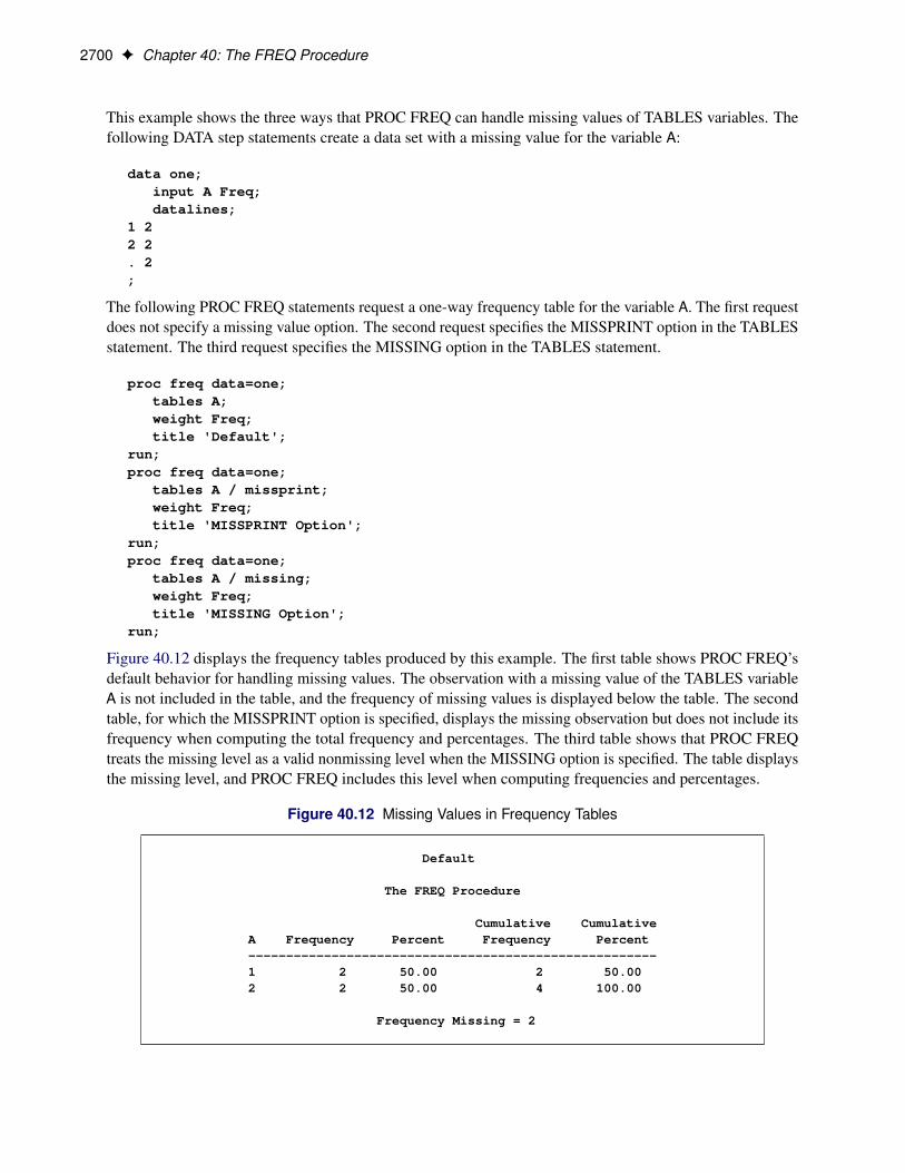
2700 F Chapter 40: The FREQ Procedure
This example shows the three ways that PROC FREQ can handle missing values of TABLES variables. Thefollowing DATA step statements create a data set with a missing value for the variable A:
data one;input A Freq;datalines;
1 22 2. 2;
The following PROC FREQ statements request a one-way frequency table for the variable A. The first requestdoes not specify a missing value option. The second request specifies the MISSPRINT option in the TABLESstatement. The third request specifies the MISSING option in the TABLES statement.
proc freq data=one;tables A;weight Freq;title 'Default';
run;proc freq data=one;
tables A / missprint;weight Freq;title 'MISSPRINT Option';
run;proc freq data=one;
tables A / missing;weight Freq;title 'MISSING Option';
run;
Figure 40.12 displays the frequency tables produced by this example. The first table shows PROC FREQ’sdefault behavior for handling missing values. The observation with a missing value of the TABLES variableA is not included in the table, and the frequency of missing values is displayed below the table. The secondtable, for which the MISSPRINT option is specified, displays the missing observation but does not include itsfrequency when computing the total frequency and percentages. The third table shows that PROC FREQtreats the missing level as a valid nonmissing level when the MISSING option is specified. The table displaysthe missing level, and PROC FREQ includes this level when computing frequencies and percentages.
Figure 40.12 Missing Values in Frequency Tables
Default
The FREQ Procedure
Cumulative CumulativeA Frequency Percent Frequency Percent------------------------------------------------------1 2 50.00 2 50.002 2 50.00 4 100.00
Frequency Missing = 2
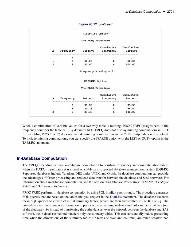
In-Database Computation F 2701
Figure 40.12 continued
MISSPRINT Option
The FREQ Procedure
Cumulative CumulativeA Frequency Percent Frequency Percent------------------------------------------------------. 2 . . .1 2 50.00 2 50.002 2 50.00 4 100.00
Frequency Missing = 2
MISSING Option
The FREQ Procedure
Cumulative CumulativeA Frequency Percent Frequency Percent------------------------------------------------------. 2 33.33 2 33.331 2 33.33 4 66.672 2 33.33 6 100.00
When a combination of variable values for a two-way table is missing, PROC FREQ assigns zero to thefrequency count for the table cell. By default, PROC FREQ does not display missing combinations in LISTformat. Also, PROC FREQ does not include missing combinations in the OUT= output data set by default.To include missing combinations, you can specify the SPARSE option with the LIST or OUT= option in theTABLES statement.
In-Database ComputationThe FREQ procedure can use in-database computation to construct frequency and crosstabulation tableswhen the DATA= input data set is stored as a table in a supported database management system (DBMS).Supported databases include Teradata, DB2 under UNIX, and Oracle. In-database computation can providethe advantages of faster processing and reduced data transfer between the database and SAS software. Forinformation about in-database computation, see the section “In-Database Procedures” in SAS/ACCESS forRelational Databases: Reference.
PROC FREQ performs in-database computation by using SQL implicit pass-through. The procedure generatesSQL queries that are based on the tables that you request in the TABLES statement. The database executesthese SQL queries to construct initial summary tables, which are then transmitted to PROC FREQ. Theprocedure uses this summary information to perform the remaining analyses and tasks in the usual way (outof the database). So instead of transferring the entire data set over the network between the database and SASsoftware, the in-database method transfers only the summary tables. This can substantially reduce processingtime when the dimensions of the summary tables (in terms of rows and columns) are much smaller than

2702 F Chapter 40: The FREQ Procedure
the dimensions of the entire database table (in terms of individual observations). Additionally, in-databasesummarization uses efficient parallel processing, which can also provide performance advantages.
In-database computation is controlled by the SQLGENERATION option, which you can specify in either aLIBNAME statement or an OPTIONS statement. See the section “In-Database Procedures” in SAS/ACCESSfor Relational Databases: Reference for details about the SQLGENERATION option and other options thataffect in-database computation. By default, PROC FREQ uses in-database computation when possible. Thereare no FREQ procedure options that control in-database computation.
PROC FREQ uses formatted values to group observations into the levels of frequency and crosstabulationtables. See the section “Grouping with Formats” on page 2698 for more information. If formats are availablein the database, then in-database summarization uses the formats. If formats are not available in the database,then in-database summarization is based on the raw data values, and PROC FREQ performs the final,formatted classification (out of the database). For more information, see the section “Deploying and UsingSAS Formats in Teradata” in SAS/ACCESS for Relational Databases: Reference.
The order of observations is not inherently defined for DBMS tables. The following options relate to theorder of observations and therefore should not be specified for PROC FREQ in-database computation:
• If you specify the FIRSTOBS= or OBS= data set option, PROC FREQ does not perform in-databasecomputation.
• If you specify the NOTSORTED option in the BY statement, PROC FREQ in-database computationignores it and uses the default ASCENDING order for BY variables.
• If you specify the ORDER=DATA option for input data in a DBMS table, PROC FREQ computationmight produce different results for separate runs of the same analysis. In addition to determining theorder of variable levels in crosstabulation table displays, the ORDER= option can also affect the valuesof many of the test statistics and measures that PROC FREQ computes.
Statistical Computations
Definitions and Notation
A two-way table represents the crosstabulation of row variable X and column variable Y. Let the table rowvalues or levels be denoted by Xi , i D 1; 2; : : : ; R, and the column values by Yj , j D 1; 2; : : : ; C . Let nijdenote the frequency of the table cell in the ith row and jth column and define the following notation:
ni � DXj
nij (row totals)
n�j DXi
nij (column totals)
n DXi
Xj
nij (overall total)
pij D nij =n (cell percentages)
pi � D ni �=n (row percentages of total)
p�j D n�j =n (column percentages of total)

Statistical Computations F 2703
Ri D score for row i
Cj D score for column j
NR DXi
ni �Ri=n (average row score)
NC DXj
n�jCj =n (average column score)
Aij DXk>i
Xl>j
nkl CXk<i
Xl<j
nkl
Dij DXk>i
Xl<j
nkl CXk<i
Xl>j
nkl
P DXi
Xj
nijAij (twice the number of concordances)
Q DXi
Xj
nijDij (twice the number of discordances)
ScoresPROC FREQ uses scores of the variable values to compute the Mantel-Haenszel chi-square, Pearsoncorrelation, Cochran-Armitage test for trend, weighted kappa coefficient, and Cochran-Mantel-Haenszelstatistics. The SCORES= option in the TABLES statement specifies the score type that PROC FREQ uses.The available score types are TABLE, RANK, RIDIT, and MODRIDIT scores. The default score type isTABLE. Using MODRIDIT, RANK, or RIDIT scores yields nonparametric analyses.
For numeric variables, table scores are the values of the row and column levels. If the row or column variableis formatted, then the table score is the internal numeric value corresponding to that level. If two or morenumeric values are classified into the same formatted level, then the internal numeric value for that level isthe smallest of these values. For character variables, table scores are defined as the row numbers and columnnumbers (that is, 1 for the first row, 2 for the second row, and so on).
Rank scores, which you request with the SCORES=RANK option, are defined as
R1i DXk<i
nk� C .ni � C 1/=2 i D 1; 2; : : : ; R
C 1j DXl<j
n�l C .n�j C 1/=2 j D 1; 2; : : : ; C
where R1i is the rank score of row i, and C 1j is the rank score of column j. Note that rank scores yieldmidranks for tied values.
Ridit scores, which you request with the SCORES=RIDIT option, are defined as rank scores standardized bythe sample size (Bross 1958; Mack and Skillings 1980). Ridit scores are derived from the rank scores as
R2i D R1i =n i D 1; 2; : : : ; R
C 2j D C1j =n j D 1; 2; : : : ; C
Modified ridit scores (SCORES=MODRIDIT) represent the expected values of the order statistics of theuniform distribution on (0,1) (van Elteren 1960; Lehmann and D’Abrera 2006). Modified ridit scores are
2704 F Chapter 40: The FREQ Procedure
derived from rank scores as
R3i D R1i =.nC 1/ i D 1; 2; : : : ; R
C 3j D C1j =.nC 1/ j D 1; 2; : : : ; C
Chi-Square Tests and Statistics
The CHISQ option provides chi-square tests of homogeneity or independence and measures of associationthat are based on the chi-square statistic. When you specify the CHISQ option in the TABLES statement,PROC FREQ computes the following chi-square tests for each two-way table: Pearson chi-square, likelihoodratio chi-square, and Mantel-Haenszel chi-square tests. PROC FREQ provides the following measures ofassociation that are based on the Pearson chi-square statistic: phi coefficient, contingency coefficient, andCramér’s V. For 2 � 2 tables, the CHISQ option also provides Fisher’s exact test and the continuity-adjustedchi-square statistic. You can request Fisher’s exact test for general R � C tables by specifying the FISHERoption in the TABLES or EXACT statement.
If you specify the CHISQ option for one-way tables, PROC FREQ provides a one-way Pearson chi-squaregoodness-of-fit test. If you specify the CHISQ(LRCHI) option for one-way tables, PROC FREQ also providesa one-way likelihood ratio chi-square test. The other tests and statistics that the CHISQ option produces areavailable only for two-way tables.
For two-way tables, the null hypothesis for the chi-square tests is no association between the row variableand the column variable. When the sample size n is large, the test statistics have asymptotic chi-squaredistributions under the null hypothesis. When the sample size is not large, or when the data set is sparseor heavily tied, exact tests might be more appropriate than asymptotic tests. PROC FREQ provides exactp-values for the Pearson chi-square, likelihood ratio chi-square, and Mantel-Haenszel chi-square tests, inaddition to Fisher’s exact test. For one-way tables, PROC FREQ provides exact p-values for the Pearsonand likelihood ratio chi-square goodness-of-fit tests. You can request these exact tests by specifying thecorresponding options in the EXACT statement. See the section “Exact Statistics” on page 2757 for moreinformation.
The Mantel-Haenszel chi-square statistic is appropriate only when both variables lie on an ordinal scale. Theother chi-square tests and statistics in this section are appropriate for either nominal or ordinal variables. Thefollowing sections give the formulas that PROC FREQ uses to compute the chi-square tests and statistics.For more information about these statistics, see Agresti (2007) and Stokes, Davis, and Koch (2012), and theother references cited.
Chi-Square Test for One-Way TablesFor one-way frequency tables, the CHISQ option in the TABLES statement provides a chi-square goodness-of-fit test. Let C denote the number of classes, or levels, in the one-way table. Let fi denote the frequencyof class i (or the number of observations in class i) for i D 1; 2; : : : ; C . Then PROC FREQ computes theone-way chi-square statistic as
QP D
CXiD1
.fi � ei /2=ei
where ei is the expected frequency for class i under the null hypothesis.
In the test for equal proportions, which is the default for the CHISQ option, the null hypothesis specifiesequal proportions of the total sample size for each class. Under this null hypothesis, the expected frequency
Statistical Computations F 2705
for each class equals the total sample size divided by the number of classes,
ei D n = C for i D 1; 2; : : : ; C
In the test for specified frequencies, which PROC FREQ computes when you input null hypothesis frequenciesby using the TESTF= option, the expected frequencies are the TESTF= values that you specify. In the test forspecified proportions, which PROC FREQ computes when you input null hypothesis proportions by usingthe TESTP= option, the expected frequencies are determined from the specified TESTP= proportions pi as
ei D pi � n for i D 1; 2; : : : ; C
Under the null hypothesis (of equal proportions, specified frequencies, or specified proportions), QP has anasymptotic chi-square distribution with C–1 degrees of freedom.
In addition to the asymptotic test, you can request an exact one-way chi-square test by specifying the CHISQoption in the EXACT statement. See the section “Exact Statistics” on page 2757 for more information.
Pearson Chi-Square Test for Two-Way TablesThe Pearson chi-square for two-way tables involves the differences between the observed and expectedfrequencies, where the expected frequencies are computed under the null hypothesis of independence. ThePearson chi-square statistic is computed as
QP DXi
Xj
.nij � eij /2=eij
where nij is the observed frequency in table cell (i, j) and eij is the expected frequency for table cell (i,j). The expected frequency is computed under the null hypothesis that the row and column variables areindependent,
eij D .ni � n�j / = n
When the row and column variables are independent, QP has an asymptotic chi-square distribution with(R–1)(C–1) degrees of freedom. For large values of QP , this test rejects the null hypothesis in favor of thealternative hypothesis of general association.
In addition to the asymptotic test, you can request an exact Pearson chi-square test by specifying the PCHIor CHISQ option in the EXACT statement. See the section “Exact Statistics” on page 2757 for moreinformation.
For 2�2 tables, the Pearson chi-square is also appropriate for testing the equality of two binomial proportions.For R � 2 and 2 � C tables, the Pearson chi-square tests the homogeneity of proportions. See Fienberg(1980) for details.
Standardized ResidualsWhen you specify the CROSSLIST(STDRES) option in the TABLES statement for two-way or multiwaytables, PROC FREQ displays the standardized residuals in the CROSSLIST table.
The standardized residual of a crosstabulation table cell is the ratio of (frequency – expected) to its standarderror, where frequency is the table cell frequency and expected is the estimated expected cell frequency. Theexpected frequency is computed under the null hypothesis that the row and column variables are independent.See the section “Pearson Chi-Square Test for Two-Way Tables” on page 2705 for more information.

2706 F Chapter 40: The FREQ Procedure
PROC FREQ computes the standardized residual of table cell (i, j) as
.nij � eij / =
qeij .1 � pi �/.1 � p�j /
where nij is the observed frequency of table cell (i, j), eij is the expected frequency of the table cell, pi � isthe proportion in row i (ni �=n), and p�j is the proportion in column j (n�j =n). The expected frequency oftable cell (i, j) is computed as
eij D .ni � n�j / = n
Under the null hypothesis of independence, each standardized residual has an asymptotic standard normaldistribution. See section 2.4.5 of Agresti (2007) for more information.
Likelihood Ratio Chi-Square Test for One-Way TablesFor one-way frequency tables, the CHISQ(LRCHI) option in the TABLES statement provides a likelihoodratio chi-square goodness-of-fit test. By default, the likelihood ratio test is based on the null hypothesis ofequal proportions in the C classes (levels) of the one-way table. If you specify null hypothesis proportions orfrequencies by using the CHISQ(TESTP=) or CHISQ(TESTF=) option, respectively, the likelihood ratio testis based on the null hypothesis values that you specify.
PROC FREQ computes the one-way likelihood ratio test as
G2 D 2
CXiD1
fi ln.fi=ei /
where fi is the observed frequency of class i, and ei is the expected frequency of class i under the nullhypothesis.
For the null hypothesis of equal proportions, the expected frequency of each class equals the total samplesize divided by the number of classes,
ei D n = C for i D 1; 2; : : : ; C
If you provide null hypothesis frequencies by specifying the CHISQ(TESTF=) option in the TABLESstatement, the expected frequencies are the TESTF= values that you specify. If you provide null hypothesisproportions by specifying the CHISQ(TESTP=) option in the TABLES statement, PROC FREQ computesthe expected frequencies as
ei D pi � n for i D 1; 2; : : : ; C
where the proportions pi are the TESTP= values that you specify.
Under the null hypothesis (of equal proportions, specified frequencies, or specified proportions), the likelihoodratio statistic G2 has an asymptotic chi-square distribution with C–1 degrees of freedom.
In addition to the asymptotic test, you can request an exact one-way likelihood ratio chi-square test byspecifying the LRCHI option in the EXACT statement. See the section “Exact Statistics” on page 2757 formore information.

Statistical Computations F 2707
Likelihood Ratio Chi-Square TestThe likelihood ratio chi-square involves the ratios between the observed and expected frequencies. Thelikelihood ratio chi-square statistic is computed as
G2 D 2Xi
Xj
nij ln�nij =eij
�where nij is the observed frequency in table cell (i, j) and eij is the expected frequency for table cell (i, j).
When the row and column variables are independent, G2 has an asymptotic chi-square distribution with(R–1)(C–1) degrees of freedom.
In addition to the asymptotic test, you can request an exact likelihood ratio chi-square test by specifying theLRCHI or CHISQ option in the EXACT statement. See the section “Exact Statistics” on page 2757 for moreinformation.
Continuity-Adjusted Chi-Square TestThe continuity-adjusted chi-square for 2 � 2 tables is similar to the Pearson chi-square, but it is adjustedfor the continuity of the chi-square distribution. The continuity-adjusted chi-square is most useful for smallsample sizes. The use of the continuity adjustment is somewhat controversial; this chi-square test is moreconservative (and more like Fisher’s exact test) when the sample size is small. As the sample size increases,the continuity-adjusted chi-square becomes more like the Pearson chi-square.
The continuity-adjusted chi-square statistic is computed as
QC DXi
Xj
�max.0; jnij � eij j � 0:5/
�2= eij
Under the null hypothesis of independence, QC has an asymptotic chi-square distribution with (R–1)(C–1)degrees of freedom.
Mantel-Haenszel Chi-Square TestThe Mantel-Haenszel chi-square statistic tests the alternative hypothesis that there is a linear associationbetween the row variable and the column variable. Both variables must lie on an ordinal scale. TheMantel-Haenszel chi-square statistic is computed as
QMH D .n � 1/r2
where r is the Pearson correlation between the row variable and the column variable. For a description ofthe Pearson correlation, see the “Pearson Correlation Coefficient” on page 2713. The Pearson correlationand thus the Mantel-Haenszel chi-square statistic use the scores that you specify in the SCORES= option inthe TABLES statement. See Mantel and Haenszel (1959) and Landis, Heyman, and Koch (1978) for moreinformation.
Under the null hypothesis of no association, QMH has an asymptotic chi-square distribution with one degreeof freedom.
In addition to the asymptotic test, you can request an exact Mantel-Haenszel chi-square test by specifyingthe MHCHI or CHISQ option in the EXACT statement. See the section “Exact Statistics” on page 2757 formore information.

2708 F Chapter 40: The FREQ Procedure
Fisher’s Exact TestFisher’s exact test is another test of association between the row and column variables. This test assumes thatthe row and column totals are fixed, and then uses the hypergeometric distribution to compute probabilitiesof possible tables conditional on the observed row and column totals. Fisher’s exact test does not depend onany large-sample distribution assumptions, and so it is appropriate even for small sample sizes and for sparsetables.
2 � 2 Tables For 2 � 2 tables, PROC FREQ gives the following information for Fisher’s exact test: tableprobability, two-sided p-value, left-sided p-value, and right-sided p-value. The table probability equals thehypergeometric probability of the observed table, and is in fact the value of the test statistic for Fisher’s exacttest.
Where p is the hypergeometric probability of a specific table with the observed row and column totals,Fisher’s exact p-values are computed by summing probabilities p over defined sets of tables,
Prob DXA
p
The two-sided p-value is the sum of all possible table probabilities (conditional on the observed row andcolumn totals) that are less than or equal to the observed table probability. For the two-sided p-value, the setA includes all possible tables with hypergeometric probabilities less than or equal to the probability of theobserved table. A small two-sided p-value supports the alternative hypothesis of association between the rowand column variables.
For 2 � 2 tables, one-sided p-values for Fisher’s exact test are defined in terms of the frequency of the cell inthe first row and first column of the table, the (1,1) cell. Denoting the observed (1,1) cell frequency by n11,the left-sided p-value for Fisher’s exact test is the probability that the (1,1) cell frequency is less than or equalto n11. For the left-sided p-value, the set A includes those tables with a (1,1) cell frequency less than or equalto n11. A small left-sided p-value supports the alternative hypothesis that the probability of an observationbeing in the first cell is actually less than expected under the null hypothesis of independent row and columnvariables.
Similarly, for a right-sided alternative hypothesis, A is the set of tables where the frequency of the (1,1) cellis greater than or equal to that in the observed table. A small right-sided p-value supports the alternative thatthe probability of the first cell is actually greater than that expected under the null hypothesis.
Because the (1,1) cell frequency completely determines the 2 � 2 table when the marginal row and columnsums are fixed, these one-sided alternatives can be stated equivalently in terms of other cell probabilities orratios of cell probabilities. The left-sided alternative is equivalent to an odds ratio less than 1, where theodds ratio equals (n11n22=n12n21). Additionally, the left-sided alternative is equivalent to the column 1 riskfor row 1 being less than the column 1 risk for row 2, p1j1 < p1j2. Similarly, the right-sided alternative isequivalent to the column 1 risk for row 1 being greater than the column 1 risk for row 2, p1j1 > p1j2. SeeAgresti (2007) for details.
R � C Tables Fisher’s exact test was extended to general R � C tables by Freeman and Halton (1951),and this test is also known as the Freeman-Halton test. For R � C tables, the two-sided p-value definitionis the same as for 2 � 2 tables. The set A contains all tables with p less than or equal to the probability ofthe observed table. A small p-value supports the alternative hypothesis of association between the row andcolumn variables. For R � C tables, Fisher’s exact test is inherently two-sided. The alternative hypothesisis defined only in terms of general, and not linear, association. Therefore, Fisher’s exact test does not haveright-sided or left-sided p-values for general R � C tables.
Statistical Computations F 2709
For R � C tables, PROC FREQ computes Fisher’s exact test by using the network algorithm of Mehta andPatel (1983), which provides a faster and more efficient solution than direct enumeration. See the section“Exact Statistics” on page 2757 for more details.
Phi CoefficientThe phi coefficient is a measure of association derived from the Pearson chi-square. The range of thephi coefficient is �1 � � � 1 for 2 � 2 tables. For tables larger than 2 � 2, the range is 0 � � �
min.pR � 1;
pC � 1/ (Liebetrau 1983). The phi coefficient is computed as
� D .n11n22 � n12n21/ =pn1�n2�n�1n�2 for 2 � 2 tables
� DpQP=n otherwise
See Fleiss, Levin, and Paik (2003, pp. 98–99) for more information.
Contingency CoefficientThe contingency coefficient is a measure of association derived from the Pearson chi-square. The rangeof the contingency coefficient is 0 � P �
p.m � 1/=m, where m D min.R; C / (Liebetrau 1983). The
contingency coefficient is computed as
P DpQP = .QP C n/
See Kendall and Stuart (1979, pp. 587–588) for more information.
Cramér’s VCramér’s V is a measure of association derived from the Pearson chi-square. It is designed so that theattainable upper bound is always 1. The range of Cramér’s V is �1 � V � 1 for 2 � 2 tables; for tableslarger than 2 � 2, the range is 0 � V � 1. Cramér’s V is computed as
V D � for 2 � 2 tables
V D
sQP=n
min.R � 1; C � 1/otherwise
See Kendall and Stuart (1979, p. 588) for more information.
Measures of Association
When you specify the MEASURES option in the TABLES statement, PROC FREQ computes severalstatistics that describe the association between the row and column variables of the contingency table. Thefollowing are measures of ordinal association that consider whether the column variable Y tends to increaseas the row variable X increases: gamma, Kendall’s tau-b, Stuart’s tau-c, and Somers’ D. These measures areappropriate for ordinal variables, and they classify pairs of observations as concordant or discordant. A pairis concordant if the observation with the larger value of X also has the larger value of Y. A pair is discordantif the observation with the larger value of X has the smaller value of Y. See Agresti (2007) and the otherreferences cited for the individual measures of association.
The Pearson correlation coefficient and the Spearman rank correlation coefficient are also appropriate forordinal variables. The Pearson correlation describes the strength of the linear association between the rowand column variables, and it is computed by using the row and column scores specified by the SCORES=option in the TABLES statement. The Spearman correlation is computed with rank scores. The polychoriccorrelation (requested by the PLCORR option) also requires ordinal variables and assumes that the variables

2710 F Chapter 40: The FREQ Procedure
have an underlying bivariate normal distribution. The following measures of association do not requireordinal variables and are appropriate for nominal variables: lambda asymmetric, lambda symmetric, and theuncertainty coefficients.
PROC FREQ computes estimates of the measures according to the formulas given in the following sections.For each measure, PROC FREQ computes an asymptotic standard error (ASE), which is the square root ofthe asymptotic variance denoted by Var in the following sections.
Confidence LimitsIf you specify the CL option in the TABLES statement, PROC FREQ computes asymptotic confidencelimits for all MEASURES statistics. The confidence coefficient is determined according to the value of theALPHA= option, which, by default, equals 0.05 and produces 95% confidence limits.
The confidence limits are computed as
Est ˙ . z˛=2 �ASE /
where Est is the estimate of the measure, z˛=2 is the 100.1 � ˛=2/ percentile of the standard normaldistribution, and ASE is the asymptotic standard error of the estimate.
Asymptotic TestsFor each measure that you specify in the TEST statement, PROC FREQ computes an asymptotic test ofthe null hypothesis that the measure equals zero. Asymptotic tests are available for the following measuresof association: gamma, Kendall’s tau-b, Stuart’s tau-c, Somers’ D.C jR/, Somers’ D.RjC/, the Pearsoncorrelation coefficient, and the Spearman rank correlation coefficient. To compute an asymptotic test, PROCFREQ uses a standardized test statistic z, which has an asymptotic standard normal distribution under thenull hypothesis. The test statistic is computed as
z D Est =p
Var0.Est/
where Est is the estimate of the measure and Var0.Est/ is the variance of the estimate under the nullhypothesis. Formulas for Var0.Est/ for the individual measures of association are given in the followingsections.
Note that the ratio of Est top
Var0.Est/ is the same for the following measures: gamma, Kendall’s tau-b,Stuart’s tau-c, Somers’ D.C jR/, and Somers’ D.RjC/. Therefore, the tests for these measures are identical.For example, the p-values for the test of H0W gamma D 0 equal the p-values for the test of H0W tau � b D 0.
PROC FREQ computes one-sided and two-sided p-values for each of these tests. When the test statistic z isgreater than its null hypothesis expected value of zero, PROC FREQ displays the right-sided p-value, whichis the probability of a larger value of the statistic occurring under the null hypothesis. A small right-sidedp-value supports the alternative hypothesis that the true value of the measure is greater than zero. When thetest statistic is less than or equal to zero, PROC FREQ displays the left-sided p-value, which is the probabilityof a smaller value of the statistic occurring under the null hypothesis. A small left-sided p-value supports thealternative hypothesis that the true value of the measure is less than zero. The one-sided p-value P1 can beexpressed as
P1 D
(Prob.Z > z/ if z > 0
Prob.Z < z/ if z � 0
where Z has a standard normal distribution. The two-sided p-value P2 is computed as
P2 D Prob.jZj > jzj/
Statistical Computations F 2711
Exact TestsExact tests are available for the following measures of association: Kendall’s tau-b, Stuart’s tau-c, Somers’D.C jR/ and .RjC/, the Pearson correlation coefficient, and the Spearman rank correlation coefficient. Ifyou request an exact test for a measure of association in the EXACT statement, PROC FREQ computes theexact test of the hypothesis that the measure equals zero. See the section “Exact Statistics” on page 2757 fordetails.
GammaThe gamma (�) statistic is based only on the number of concordant and discordant pairs of observations. Itignores tied pairs (that is, pairs of observations that have equal values of X or equal values of Y). Gamma isappropriate only when both variables lie on an ordinal scale. The range of gamma is �1 � � � 1. If the rowand column variables are independent, then gamma tends to be close to zero. Gamma is computed as
G D .P �Q/ = .P CQ/
and the asymptotic variance is
Var.G/ D16
.P CQ/4
Xi
Xj
nij .QAij � PDij /2
For 2 � 2 tables, gamma is equivalent to Yule’s Q. See Goodman and Kruskal (1979) and Agresti (2002) formore information.
The variance under the null hypothesis that gamma equals zero is computed as
Var0.G/ D4
.P CQ/2
0@Xi
Xj
nij .Aij �Dij /2� .P �Q/2=n
1ASee Brown and Benedetti (1977) for details.
Kendall’s Tau-bKendall’s tau-b (�b) is similar to gamma except that tau-b uses a correction for ties. Tau-b is appropriate onlywhen both variables lie on an ordinal scale. The range of tau-b is �1 � �b � 1. Kendall’s tau-b is computedas
tb D .P �Q/ =pwrwc
and the asymptotic variance is
Var.tb/ D1
w4
0@Xi
Xj
nij .2wdij C tbvij /2� n3t2b .wr C wc/
2
1Awhere
w Dpwrwc
wr D n2 �Xi
n2i �
wc D n2 �Xj
n2�j
dij D Aij �Dij
vij D ni �wc C n�jwr
2712 F Chapter 40: The FREQ Procedure
See Kendall (1955) for more information.
The variance under the null hypothesis that tau-b equals zero is computed as
Var0.tb/ D4
wrwc
0@Xi
Xj
nij .Aij �Dij /2� .P �Q/2=n
1ASee Brown and Benedetti (1977) for details.
PROC FREQ also provides an exact test for the Kendall’s tau-b. You can request this test by specifyingthe KENTB option in the EXACT statement. See the section “Exact Statistics” on page 2757 for moreinformation.
Stuart’s Tau-cStuart’s tau-c (�c) makes an adjustment for table size in addition to a correction for ties. Tau-c is appropriateonly when both variables lie on an ordinal scale. The range of tau-c is �1 � �c � 1. Stuart’s tau-c iscomputed as
tc D m.P �Q/ = n2.m � 1/
and the asymptotic variance is
Var.tc/ D4m2
.m � 1/2n4
0@Xi
Xj
nijd2ij � .P �Q/
2=n
1Awhere m D min.R; C / and dij D Aij �Dij . The variance under the null hypothesis that tau-c equals zerois the same as the asymptotic variance Var,
Var0.tc/ D Var.tc/
See Brown and Benedetti (1977) for details.
PROC FREQ also provides an exact test for the Stuart’s tau-c. You can request this test by specifyingthe STUTC option in the EXACT statement. See the section “Exact Statistics” on page 2757 for moreinformation.
Somers’ DSomers’ D.C jR/ and Somers’ D.RjC/ are asymmetric modifications of tau-b. C jR indicates that therow variable X is regarded as the independent variable and the column variable Y is regarded as dependent.Similarly, RjC indicates that the column variable Y is regarded as the independent variable and the rowvariable X is regarded as dependent. Somers’ D differs from tau-b in that it uses a correction only for pairsthat are tied on the independent variable. Somers’ D is appropriate only when both variables lie on an ordinalscale. The range of Somers’ D is �1 � D � 1. Somers’ D.C jR/ is computed as
D.C jR/ D .P �Q/ = wr
and its asymptotic variance is
Var.D.C jR// D4
w4r
Xi
Xj
nij�wrdij � .P �Q/.n � ni �/
�2

Statistical Computations F 2713
where dij D Aij �Dij and
wr D n2�
Xi
n2i �
For more information, see Somers (1962); Goodman and Kruskal (1979); Liebetrau (1983).
The variance under the null hypothesis that D.C jR/ equals zero is computed as
Var0.D.C jR// D4
w2r
0@Xi
Xj
nij .Aij �Dij /2� .P �Q/2=n
1ASee Brown and Benedetti (1977) for details.
Formulas for Somers’ D.RjC/ are obtained by interchanging the indices.
PROC FREQ also provides exact tests for Somers’ D.C jR/ and .RjC/. You can request these tests byspecifying the SMDCR and SMDCR options in the EXACT statement. See the section “Exact Statistics” onpage 2757 for more information.
Pearson Correlation CoefficientThe Pearson correlation coefficient (�) is computed by using the scores specified in the SCORES= option.This measure is appropriate only when both variables lie on an ordinal scale. The range of the Pearsoncorrelation is �1 � � � 1. The Pearson correlation coefficient is computed as
r D v=w D ssrc=p
ssrssc
and its asymptotic variance is
Var.r/ D1
w4
Xi
Xj
nij
�w.Ri � NR/.Cj � NC/ �
bij v
2w
�2where Ri and Cj are the row and column scores and
ssr DXi
Xj
nij .Ri � NR/2
ssc DXi
Xj
nij .Cj � NC/2
ssrc DXi
Xj
nij .Ri � NR/.Cj � NC/
bij D .Ri � NR/2ssc C .Cj � NC/2ssr
v D ssrc
w Dp
ssrssc
See Snedecor and Cochran (1989) for more information.
2714 F Chapter 40: The FREQ Procedure
The SCORES= option in the TABLES statement determines the type of row and column scores used tocompute the Pearson correlation (and other score-based statistics). The default is SCORES=TABLE. See thesection “Scores” on page 2703 for details about the available score types and how they are computed.
The variance under the null hypothesis that the correlation equals zero is computed as
Var0.r/ D
0@Xi
Xj
nij .Ri � NR/2.Cj � NC/
2� ss2rc=n
1A = ssrssc
Note that this expression for the variance is derived for multinomial sampling in a contingency tableframework, and it differs from the form obtained under the assumption that both variables are continuous andnormally distributed. See Brown and Benedetti (1977) for details.
PROC FREQ also provides an exact test for the Pearson correlation coefficient. You can request this test byspecifying the PCORR option in the EXACT statement. See the section “Exact Statistics” on page 2757 formore information.
Spearman Rank Correlation CoefficientThe Spearman correlation coefficient (�s) is computed by using rank scores, which are defined in the section“Scores” on page 2703. This measure is appropriate only when both variables lie on an ordinal scale. Therange of the Spearman correlation is �1 � �s � 1. The Spearman correlation coefficient is computed as
rs D v = w
and its asymptotic variance is
Var.rs/ D1
n2w4
Xi
Xj
nij .zij � Nz/2
where R1i and C 1j are the row and column rank scores and
v DXi
Xj
nijR.i/C.j /
w D1
12
pFG
F D n3 �Xi
n3i �
G D n3 �Xj
n3�j
R.i/ D R1i � n=2
C.j / D C 1j � n=2
Nz D1
n
Xi
Xj
nij zij
zij D wvij � vwij

Statistical Computations F 2715
vij D n
R.i/C.j / C
1
2
Xl
nilC.l/ C1
2
Xk
nkjR.k/C
Xl
Xk>i
nklC.l/ CXk
Xl>j
nklR.k/
1Awij D
�n
96w
�Fn2�j CGn
2i �
�See Snedecor and Cochran (1989) for more information.
The variance under the null hypothesis that the correlation equals zero is computed as
Var0.rs/ D1
n2w2
Xi
Xj
nij .vij � Nv/2
where
Nv DXi
Xj
nij vij =n
Note that the asymptotic variance is derived for multinomial sampling in a contingency table framework,and it differs from the form obtained under the assumption that both variables are continuous and normallydistributed. See Brown and Benedetti (1977) for details.
PROC FREQ also provides an exact test for the Spearman correlation coefficient. You can request this test byspecifying the SCORR option in the EXACT statement. See the section “Exact Statistics” on page 2757 formore information.
Polychoric CorrelationWhen you specify the PLCORR option in the TABLES statement, PROC FREQ computes the polychoriccorrelation and its standard error. The polychoric correlation is based on the assumption that the two ordinal,categorical variables of the frequency table have an underlying bivariate normal distribution. The polychoriccorrelation coefficient is the maximum likelihood estimate of the product-moment correlation between theunderlying normal variables. The range of the polychoric correlation is from –1 to 1. For 2 � 2 tables, thepolychoric correlation is also known as the tetrachoric correlation (and it is labeled as such in the displayedoutput). See Drasgow (1986) for an overview of polychoric correlation coefficient.
Olsson (1979) gives the likelihood equations and the asymptotic standard errors for estimating the polychoriccorrelation. The underlying continuous variables relate to the observed crosstabulation table throughthresholds, which define a range of numeric values that correspond to each categorical (table) level. PROCFREQ uses Olsson’s maximum likelihood method for simultaneous estimation of the polychoric correlationand the thresholds. (Olsson also presents a two-step method that estimates the thresholds first.)
PROC FREQ iteratively solves the likelihood equations by using a Newton-Raphson algorithm. Theinitial estimates of the thresholds are computed from the inverse of the normal distribution function at thecumulative marginal proportions of the table. Iterative computation of the polychoric correlation stops whenthe convergence measure falls below the convergence criterion or when the maximum number of iterationsis reached, whichever occurs first. For parameter values that are less than 0.01, the procedure evaluatesconvergence by using the absolute difference instead of the relative difference. The PLCORR(CONVERGE=)
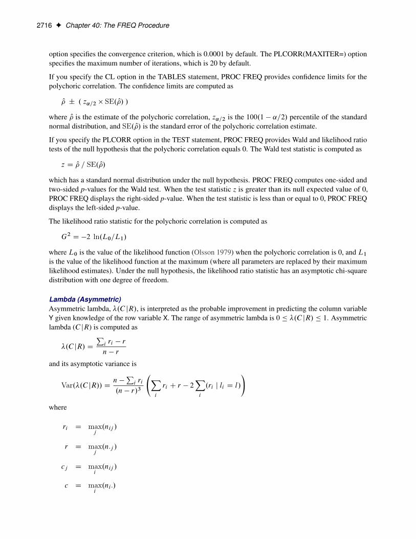
2716 F Chapter 40: The FREQ Procedure
option specifies the convergence criterion, which is 0.0001 by default. The PLCORR(MAXITER=) optionspecifies the maximum number of iterations, which is 20 by default.
If you specify the CL option in the TABLES statement, PROC FREQ provides confidence limits for thepolychoric correlation. The confidence limits are computed as
O� ˙ . z˛=2 � SE. O�/ /
where O� is the estimate of the polychoric correlation, z˛=2 is the 100.1 � ˛=2/ percentile of the standardnormal distribution, and SE. O�/ is the standard error of the polychoric correlation estimate.
If you specify the PLCORR option in the TEST statement, PROC FREQ provides Wald and likelihood ratiotests of the null hypothesis that the polychoric correlation equals 0. The Wald test statistic is computed as
z D O� = SE. O�/
which has a standard normal distribution under the null hypothesis. PROC FREQ computes one-sided andtwo-sided p-values for the Wald test. When the test statistic z is greater than its null expected value of 0,PROC FREQ displays the right-sided p-value. When the test statistic is less than or equal to 0, PROC FREQdisplays the left-sided p-value.
The likelihood ratio statistic for the polychoric correlation is computed as
G2 D �2 ln.L0=L1/
where L0 is the value of the likelihood function (Olsson 1979) when the polychoric correlation is 0, and L1is the value of the likelihood function at the maximum (where all parameters are replaced by their maximumlikelihood estimates). Under the null hypothesis, the likelihood ratio statistic has an asymptotic chi-squaredistribution with one degree of freedom.
Lambda (Asymmetric)Asymmetric lambda, �.C jR/, is interpreted as the probable improvement in predicting the column variableY given knowledge of the row variable X. The range of asymmetric lambda is 0 � �.C jR/ � 1. Asymmetriclambda (C jR) is computed as
�.C jR/ D
Pi ri � r
n � r
and its asymptotic variance is
Var.�.C jR// Dn �
Pi ri
.n � r/3
Xi
ri C r � 2Xi
.ri j li D l/
!
where
ri D maxj.nij /
r D maxj.n�j /
cj D maxi.nij /
c D maxi.ni �/

Statistical Computations F 2717
The values of li and l are determined as follows. Denote by li the unique value of j such that ri D nij , and letl be the unique value of j such that r D n�j . Because of the uniqueness assumptions, ties in the frequenciesor in the marginal totals must be broken in an arbitrary but consistent manner. In case of ties, l is defined asthe smallest value of j such that r D n�j .
For those columns containing a cell (i, j) for which nij D ri D cj , csj records the row in which cj isassumed to occur. Initially csj is set equal to –1 for all j. Beginning with i=1, if there is at least one value jsuch that nij D ri D cj , and if csj D �1, then li is defined to be the smallest such value of j, and csj is setequal to i. Otherwise, if nil D ri , then li is defined to be equal to l. If neither condition is true, then li istaken to be the smallest value of j such that nij D ri .
The formulas for lambda asymmetric .RjC/ can be obtained by interchanging the indices.
See Goodman and Kruskal (1979) for more information.
Lambda (Symmetric)The nondirectional lambda is the average of the two asymmetric lambdas, �.C jR/ and �.RjC/. Its range is0 � � � 1. Lambda symmetric is computed as
� D
Pi ri C
Pj cj � r � c
2n � r � cDw � v
w
and its asymptotic variance is computed as
Var.�/ D1
w4
�wvy � 2w2
�n �
Xi
Xj
.nij j j D li ; i D kj /�� 2v2.n � nkl/
�where
ri D maxj.nij /
r D maxj.n�j /
cj D maxi.nij /
c D maxi.ni �/
w D 2n � r � c
v D 2n �Xi
ri �Xj
cj
x D
Xi
.ri j li D l/ CXj
.cj j kj D k/ C rk C cl
y D 8n � w � v � 2x
The definitions of li and l are given in the previous section. The values kj and k are defined in a similar wayfor lambda asymmetric (RjC ).
See Goodman and Kruskal (1979) for more information.
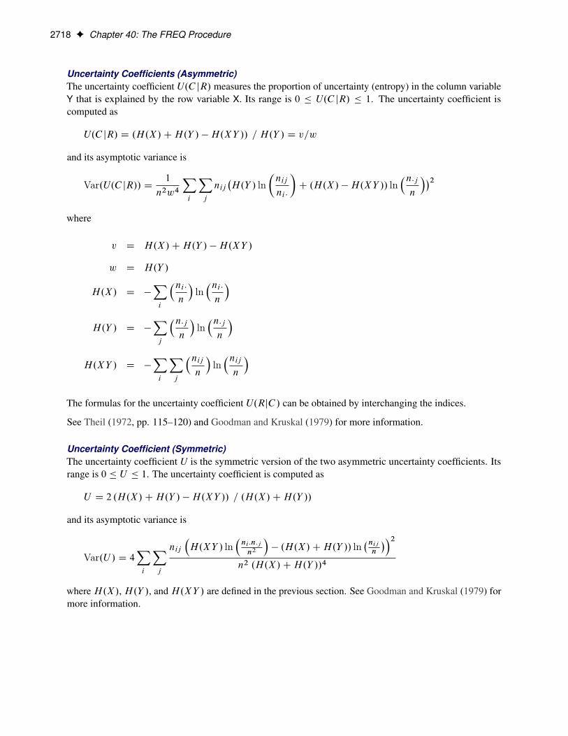
2718 F Chapter 40: The FREQ Procedure
Uncertainty Coefficients (Asymmetric)The uncertainty coefficient U.C jR/ measures the proportion of uncertainty (entropy) in the column variableY that is explained by the row variable X. Its range is 0 � U.C jR/ � 1. The uncertainty coefficient iscomputed as
U.C jR/ D .H.X/CH.Y / �H.XY // = H.Y / D v=w
and its asymptotic variance is
Var.U.C jR// D1
n2w4
Xi
Xj
nij�H.Y / ln
�nij
ni �
�C .H.X/ �H.XY // ln
�n�jn
��2where
v D H.X/CH.Y / �H.XY /
w D H.Y /
H.X/ D �
Xi
�ni �n
�ln�ni �n
�H.Y / D �
Xj
�n�jn
�ln�n�jn
�
H.XY / D �
Xi
Xj
�nijn
�ln�nijn
�
The formulas for the uncertainty coefficient U.RjC/ can be obtained by interchanging the indices.
See Theil (1972, pp. 115–120) and Goodman and Kruskal (1979) for more information.
Uncertainty Coefficient (Symmetric)The uncertainty coefficient U is the symmetric version of the two asymmetric uncertainty coefficients. Itsrange is 0 � U � 1. The uncertainty coefficient is computed as
U D 2 .H.X/CH.Y / �H.XY // = .H.X/CH.Y //
and its asymptotic variance is
Var.U / D 4Xi
Xj
nij
�H.XY / ln
�ni �n�jn2
�� .H.X/CH.Y // ln
�nij
n
��2n2 .H.X/CH.Y //4
where H.X/, H.Y /, and H.XY / are defined in the previous section. See Goodman and Kruskal (1979) formore information.

Statistical Computations F 2719
Binomial Proportion
If you specify the BINOMIAL option in the TABLES statement, PROC FREQ computes the binomialproportion for one-way tables. By default, this is the proportion of observations in the first variable level thatappears in the output. (You can use the LEVEL= option to specify a different level for the proportion.) Thebinomial proportion is computed as
Op D n1 = n
where n1 is the frequency of the first (or designated) level and n is the total frequency of the one-way table.The standard error of the binomial proportion is computed as
se. Op/ DpOp .1 � Op/ = n
Binomial Confidence LimitsBy default, PROC FREQ provides Wald and exact (Clopper-Pearson) confidence limits for the binomialproportion. If you do not specify any confidence limit requests with the CL= binomial-option, PROC FREQcomputes Wald asymptotic confidence limits. You can also request Agresti-Coull, Jeffreys, and Wilson(score) confidence limits for the binomial proportion. For details about these binomial confidence limits,including comparisons of their performance, see Brown, Cai, and DasGupta (2001); Agresti and Coull (1998);Newcombe (1998b).
Wald Confidence Limits Wald asymptotic confidence limits are based on the normal approximation tothe binomial distribution. PROC FREQ computes the Wald confidence limits for the binomial proportion as
Op ˙ . z˛=2 � se. Op/ /
where z˛=2 is the 100.1 � ˛=2/ percentile of the standard normal distribution. The confidence level ˛ isdetermined by the ALPHA= option, which, by default, equals 0.05 and produces 95% confidence limits.
If you specify CL=WALD(CORRECT) or the CORRECT binomial-option, PROC FREQ includes a continuitycorrection of 1=2n in the Wald asymptotic confidence limits. The purpose of this correction is to adjust forthe difference between the normal approximation and the discrete binomial distribution. See Fleiss, Levin,and Paik (2003) for more information. The continuity-corrected Wald confidence limits for the binomialproportion are computed as
Op ˙ . z˛=2 � se. Op/ C .1=2n/ /
Agresti-Coull Confidence Limits If you specify the CL=AGRESTICOULL binomial-option, PROCFREQ computes Agresti-Coull confidence limits for the binomial proportion as
Qp ˙ . z˛=2 �pQp .1 � Qp/ = Qn /
where
Qn1 D n1 C z2˛=2=2
Qn D nC z2˛=2
Qp D Qn1 = Qn
The Agresti-Coull confidence interval has the same general form as the standard Wald interval but uses Qpin place of Op. For ˛ D 0:05, the value of z˛=2 is close to 2, and this interval is the “add 2 successes and 2failures” adjusted Wald interval of Agresti and Coull (1998).

2720 F Chapter 40: The FREQ Procedure
Jeffreys Confidence Limits If you specify the CL=JEFFREYS binomial-option, PROC FREQ computesJeffreys confidence limits for the binomial proportion as�
ˇ.˛=2; n1 C 1=2; n � n1 C 1=2/; ˇ.1 � ˛=2; n1 C 1=2; n � n1 C 1=2/�
where ˇ.˛; b; c/ is the ˛ percentile of the beta distribution with shape parameters b and c. The lowerconfidence limit is set to 0 when n1 D 0, and the upper confidence limit is set to 1 when n1 D n. This is anequal-tailed interval based on the noninformative Jeffreys prior for a binomial proportion. See Brown, Cai,and DasGupta (2001) for details. See Berger (1985) for information about using beta priors for inference onthe binomial proportion.
Wilson (Score) Confidence Limits If you specify the CL=WILSON binomial-option, PROC FREQcomputes Wilson confidence limits for the binomial proportion. These are also known as score confidencelimits (Wilson 1927). The confidence limits are based on inverting the normal test that uses the null proportionin the variance (the score test). Wilson confidence limits are the roots of
jp � Opj D z˛=2pp.1 � p/=n
and are computed as Op C z2˛=2=2n ˙ z˛=2
r�Op.1 � Op/C z2
˛=2=4n
�=n
!=�1C z2˛=2=n
�
If you specify CL=WILSON(CORRECT) or the CORRECT binomial-option, PROC FREQ providescontinuity-corrected Wilson confidence limits, which are computed as the roots of
jp � Opj � 1=2n D z˛=2pp.1 � p/=n
The Wilson interval has been shown to have better performance than the Wald interval and the exact (Clopper-Pearson) interval. For more information, see Agresti and Coull (1998); Brown, Cai, and DasGupta (2001);Newcombe (1998b).
Exact (Clopper-Pearson) Confidence Limits Exact (Clopper-Pearson) confidence limits for the binomialproportion are constructed by inverting the equal-tailed test based on the binomial distribution. This methodis attributed to Clopper and Pearson (1934). The exact confidence limits pL and pU satisfy the followingequations, for n1 D 1; 2; : : : n � 1:
nXxDn1
n
x
!p x
L .1 � pL/n�x
D ˛=2
n1XxD0
n
x
!p x
U .1 � pU /n�x
D ˛=2
The lower confidence limit equals 0 when n1 D 0, and the upper confidence limit equals 1 when n1 D n.

Statistical Computations F 2721
PROC FREQ computes the exact (Clopper-Pearson) confidence limits by using the F distribution as
pL D
�1C
n � n1 C 1
n1 F. ˛=2; 2n1; 2.n � n1 C 1/ /
��1
pU D
�1C
n � n1
.n1 C 1/ F. 1 � ˛=2; 2.n1 C 1/; 2.n � n1/ /
��1where F.˛=2; b; c/ is the ˛=2 percentile of the F distribution with b and c degrees of freedom. See Leemisand Trivedi (1996) for a derivation of this expression. Also see Collett (1991) for more information aboutexact binomial confidence limits.
Because this is a discrete problem, the confidence coefficient (coverage probability) of the exact (Clopper-Pearson) interval is not exactly .1 � ˛/ but is at least .1 � ˛/. Thus, this confidence interval is conservative.Unless the sample size is large, the actual coverage probability can be much larger than the target value. Formore information about the performance of these confidence limits, see Agresti and Coull (1998); Brown,Cai, and DasGupta (2001); Leemis and Trivedi (1996).
Binomial TestsThe BINOMIAL option provides an asymptotic equality test for the binomial proportion by default. You canalso specify binomial-options to request tests of noninferiority, superiority, and equivalence for the binomialproportion. If you specify the BINOMIAL option in the EXACT statement, PROC FREQ also computesexact p-values for the tests that you request with the binomial-options.
Equality Test PROC FREQ computes an asymptotic test of the hypothesis that the binomial proportionequals p0, where you can specify the value of p0 with the P= binomial-option. If you do not specify a nullvalue with P=, PROC FREQ uses p0 D 0:5 by default. The binomial test statistic is computed as
z D . Op � p0/=se
By default, the standard error is based on the null hypothesis proportion as
se Dpp0.1 � p0/=n
If you specify the VAR=SAMPLE binomial-option, the standard error is computed from the sample proportionas
se DpOp.1 � Op/=n
If you specify the CORRECT binomial-option, PROC FREQ includes a continuity correction in the asymptotictest statistic, towards adjusting for the difference between the normal approximation and the discrete binomialdistribution. See Fleiss, Levin, and Paik (2003) for details. The continuity correction of .1=2n/ is subtractedfrom the numerator of the test statistic if . Op � p0/ is positive; otherwise, the continuity correction is added tothe numerator.
PROC FREQ computes one-sided and two-sided p-values for this test. When the test statistic z is greater thanzero (its expected value under the null hypothesis), PROC FREQ computes the right-sided p-value, whichis the probability of a larger value of the statistic occurring under the null hypothesis. A small right-sidedp-value supports the alternative hypothesis that the true value of the proportion is greater than p0. When
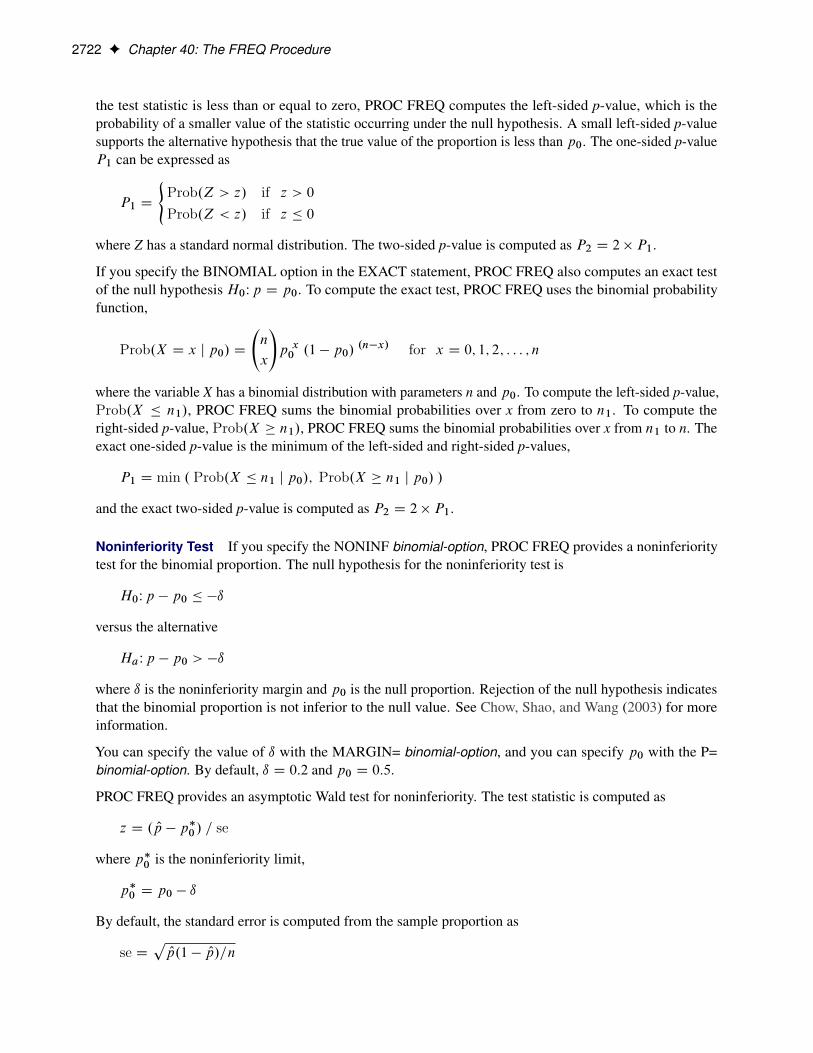
2722 F Chapter 40: The FREQ Procedure
the test statistic is less than or equal to zero, PROC FREQ computes the left-sided p-value, which is theprobability of a smaller value of the statistic occurring under the null hypothesis. A small left-sided p-valuesupports the alternative hypothesis that the true value of the proportion is less than p0. The one-sided p-valueP1 can be expressed as
P1 D
(Prob.Z > z/ if z > 0
Prob.Z < z/ if z � 0
where Z has a standard normal distribution. The two-sided p-value is computed as P2 D 2 � P1.
If you specify the BINOMIAL option in the EXACT statement, PROC FREQ also computes an exact testof the null hypothesis H0Wp D p0. To compute the exact test, PROC FREQ uses the binomial probabilityfunction,
Prob.X D x j p0/ D
n
x
!p x0 .1 � p0/
.n�x/ for x D 0; 1; 2; : : : ; n
where the variable X has a binomial distribution with parameters n and p0. To compute the left-sided p-value,Prob.X � n1/, PROC FREQ sums the binomial probabilities over x from zero to n1. To compute theright-sided p-value, Prob.X � n1/, PROC FREQ sums the binomial probabilities over x from n1 to n. Theexact one-sided p-value is the minimum of the left-sided and right-sided p-values,
P1 D min . Prob.X � n1 j p0/; Prob.X � n1 j p0/ /
and the exact two-sided p-value is computed as P2 D 2 � P1.
Noninferiority Test If you specify the NONINF binomial-option, PROC FREQ provides a noninferioritytest for the binomial proportion. The null hypothesis for the noninferiority test is
H0Wp � p0 � �ı
versus the alternative
HaWp � p0 > �ı
where ı is the noninferiority margin and p0 is the null proportion. Rejection of the null hypothesis indicatesthat the binomial proportion is not inferior to the null value. See Chow, Shao, and Wang (2003) for moreinformation.
You can specify the value of ı with the MARGIN= binomial-option, and you can specify p0 with the P=binomial-option. By default, ı D 0:2 and p0 D 0:5.
PROC FREQ provides an asymptotic Wald test for noninferiority. The test statistic is computed as
z D . Op � p�0 / = se
where p�0 is the noninferiority limit,
p�0 D p0 � ı
By default, the standard error is computed from the sample proportion as
se DpOp.1 � Op/=n

Statistical Computations F 2723
If you specify the VAR=NULL binomial-option, the standard error is based on the noninferiority limit(determined by the null proportion and the margin) as
se Dqp�0 .1 � p
�0 /=n
If you specify the CORRECT binomial-option, PROC FREQ includes a continuity correction in the asymptotictest statistic z. The continuity correction of .1=2n/ is subtracted from the numerator of the test statistic if. Op � p�0 / is positive; otherwise, the continuity correction is added to the numerator.
The p-value for the noninferiority test is
Pz D Prob.Z > z/
where Z has a standard normal distribution.
As part of the noninferiority analysis, PROC FREQ provides asymptotic Wald confidence limits for thebinomial proportion. These confidence limits are computed as described in the section “Wald ConfidenceLimits” on page 2719 but use the same standard error (VAR=NULL or VAR=SAMPLE) as the noninferioritytest statistic z. The confidence coefficient is 100.1 � 2˛/% (Schuirmann 1999). By default, if you do notspecify the ALPHA= option, the noninferiority confidence limits are 90% confidence limits. You can comparethe confidence limits to the noninferiority limit, p�0 D p0 � ı.
If you specify the BINOMIAL option in the EXACT statement, PROC FREQ provides an exact noninferioritytest for the binomial proportion. The exact p-value is computed by using the binomial probability functionwith parameters p�0 and n,
Px D
kDnXkDn1
n
k
!.p�0 /
k .1 � p�0 /.n�k/
See Chow, Shao, and Wang (2003, p. 116) for details. If you request exact binomial statistics, PROCFREQ also includes exact (Clopper-Pearson) confidence limits for the binomial proportion in the equivalenceanalysis display. See the section “Exact (Clopper-Pearson) Confidence Limits” on page 2720 for details.
Superiority Test If you specify the SUP binomial-option, PROC FREQ provides a superiority test for thebinomial proportion. The null hypothesis for the superiority test is
H0Wp � p0 � ı
versus the alternative
HaWp � p0 > ı
where ı is the superiority margin and p0 is the null proportion. Rejection of the null hypothesis indicates thatthe binomial proportion is superior to the null value. You can specify the value of ı with the MARGIN=binomial-option, and you can specify the value of p0 with the P= binomial-option. By default, ı D 0:2 andp0 D 0:5.
The superiority analysis is identical to the noninferiority analysis but uses a positive value of the margin ı inthe null hypothesis. The superiority limit equals p0 C ı. The superiority computations follow those in thesection “Noninferiority Test” on page 2722 but replace –ı with ı. See Chow, Shao, and Wang (2003) formore information.
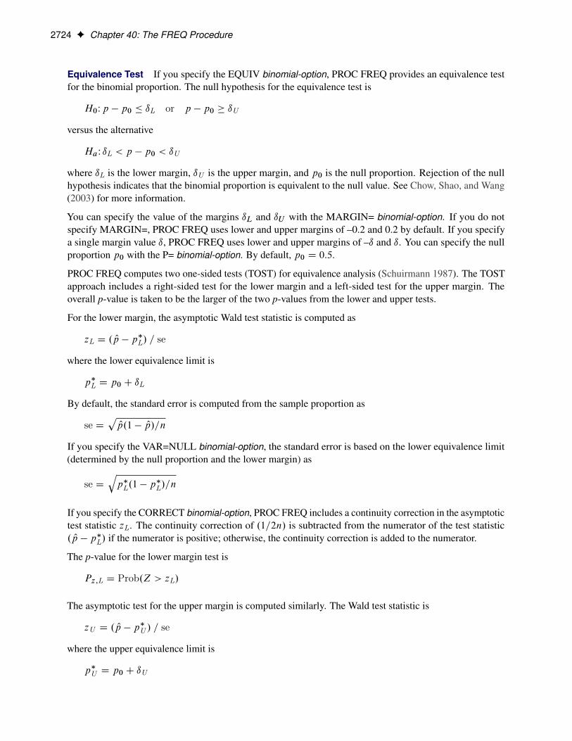
2724 F Chapter 40: The FREQ Procedure
Equivalence Test If you specify the EQUIV binomial-option, PROC FREQ provides an equivalence testfor the binomial proportion. The null hypothesis for the equivalence test is
H0Wp � p0 � ıL or p � p0 � ıU
versus the alternative
HaW ıL < p � p0 < ıU
where ıL is the lower margin, ıU is the upper margin, and p0 is the null proportion. Rejection of the nullhypothesis indicates that the binomial proportion is equivalent to the null value. See Chow, Shao, and Wang(2003) for more information.
You can specify the value of the margins ıL and ıU with the MARGIN= binomial-option. If you do notspecify MARGIN=, PROC FREQ uses lower and upper margins of –0.2 and 0.2 by default. If you specifya single margin value ı, PROC FREQ uses lower and upper margins of –ı and ı. You can specify the nullproportion p0 with the P= binomial-option. By default, p0 D 0:5.
PROC FREQ computes two one-sided tests (TOST) for equivalence analysis (Schuirmann 1987). The TOSTapproach includes a right-sided test for the lower margin and a left-sided test for the upper margin. Theoverall p-value is taken to be the larger of the two p-values from the lower and upper tests.
For the lower margin, the asymptotic Wald test statistic is computed as
zL D . Op � p�L/ = se
where the lower equivalence limit is
p�L D p0 C ıL
By default, the standard error is computed from the sample proportion as
se DpOp.1 � Op/=n
If you specify the VAR=NULL binomial-option, the standard error is based on the lower equivalence limit(determined by the null proportion and the lower margin) as
se Dqp�L.1 � p
�L/=n
If you specify the CORRECT binomial-option, PROC FREQ includes a continuity correction in the asymptotictest statistic zL. The continuity correction of .1=2n/ is subtracted from the numerator of the test statistic. Op � p�L/ if the numerator is positive; otherwise, the continuity correction is added to the numerator.
The p-value for the lower margin test is
Pz;L D Prob.Z > zL/
The asymptotic test for the upper margin is computed similarly. The Wald test statistic is
zU D . Op � p�U / = se
where the upper equivalence limit is
p�U D p0 C ıU

Statistical Computations F 2725
By default, the standard error is computed from the sample proportion. If you specify the VAR=NULLbinomial-option, the standard error is based on the upper equivalence limit as
se Dqp�U .1 � p
�U /=n
If you specify the CORRECT binomial-option, PROC FREQ includes a continuity correction of .1=2n/ inthe asymptotic test statistic zU .
The p-value for the upper margin test is
Pz;U D Prob.Z < zU /
Based on the two one-sided tests (TOST), the overall p-value for the test of equivalence equals the largerp-value from the lower and upper margin tests, which can be expressed as
Pz D max.Pz;L ; Pz;U /
As part of the equivalence analysis, PROC FREQ provides asymptotic Wald confidence limits for the binomialproportion. These confidence limits are computed as described in the section “Wald Confidence Limits” onpage 2719, but use the same standard error (VAR=NULL or VAR=SAMPLE) as the equivalence test statisticsand have a confidence coefficient of 100.1 � 2˛/% (Schuirmann 1999). By default, if you do not specify theALPHA= option, the equivalence confidence limits are 90% limits. If you specify VAR=NULL, separatestandard errors are computed for the lower and upper margin tests, each based on the null proportion and thecorresponding (lower or upper) margin. The confidence limits are computed by using the maximum of thesetwo standard errors. You can compare the confidence limits to the equivalence limits, .p0 C ıL; p0 C ıU /.
If you specify the BINOMIAL option in the EXACT statement, PROC FREQ also provides an exactequivalence test by using two one-sided exact tests (TOST). The procedure computes lower and uppermargin exact tests by using the binomial probability function as described in the section “NoninferiorityTest” on page 2722. The overall exact p-value for the equivalence test is taken to be the larger p-valuefrom the lower and upper margin exact tests. If you request exact statistics, PROC FREQ also includesexact (Clopper-Pearson) confidence limits in the equivalence analysis display. The confidence coefficientis 100.1 � 2˛/% (Schuirmann 1999). See the section “Exact (Clopper-Pearson) Confidence Limits” onpage 2720 for details.
Risks and Risk Differences
The RISKDIFF option in the TABLES statement provides estimates of risks (binomial proportions) andrisk differences for 2 � 2 tables. This analysis might be appropriate when comparing the proportion ofsome characteristic for two groups, where row 1 and row 2 correspond to the two groups, and the columnscorrespond to two possible characteristics or outcomes. For example, the row variable might be a treatmentor dose, and the column variable might be the response. For more information, see Collett (1991); Fleiss,Levin, and Paik (2003); Stokes, Davis, and Koch (2012).
Let the frequencies of the 2 � 2 table be represented as follows.
Column 1 Column 2 TotalRow 1 n11 n12 n1�Row 2 n21 n22 n2�Total n�1 n�2 n
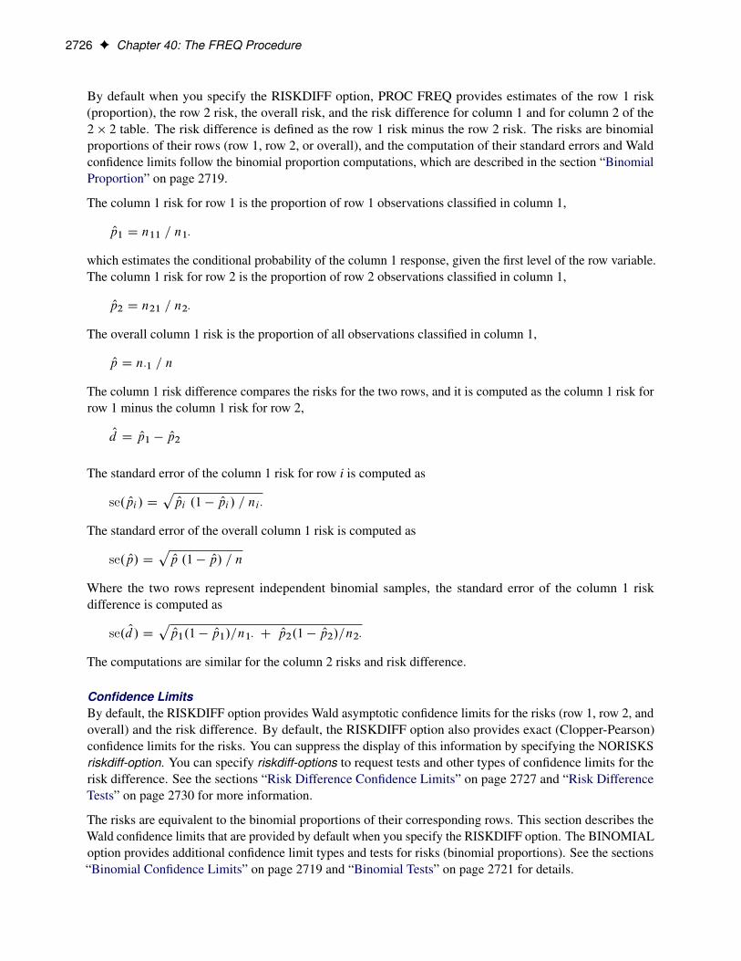
2726 F Chapter 40: The FREQ Procedure
By default when you specify the RISKDIFF option, PROC FREQ provides estimates of the row 1 risk(proportion), the row 2 risk, the overall risk, and the risk difference for column 1 and for column 2 of the2 � 2 table. The risk difference is defined as the row 1 risk minus the row 2 risk. The risks are binomialproportions of their rows (row 1, row 2, or overall), and the computation of their standard errors and Waldconfidence limits follow the binomial proportion computations, which are described in the section “BinomialProportion” on page 2719.
The column 1 risk for row 1 is the proportion of row 1 observations classified in column 1,
Op1 D n11 = n1�
which estimates the conditional probability of the column 1 response, given the first level of the row variable.The column 1 risk for row 2 is the proportion of row 2 observations classified in column 1,
Op2 D n21 = n2�
The overall column 1 risk is the proportion of all observations classified in column 1,
Op D n�1 = n
The column 1 risk difference compares the risks for the two rows, and it is computed as the column 1 risk forrow 1 minus the column 1 risk for row 2,
Od D Op1 � Op2
The standard error of the column 1 risk for row i is computed as
se. Opi / DpOpi .1 � Opi / = ni �
The standard error of the overall column 1 risk is computed as
se. Op/ DpOp .1 � Op/ = n
Where the two rows represent independent binomial samples, the standard error of the column 1 riskdifference is computed as
se. Od/ DpOp1.1 � Op1/=n1� C Op2.1 � Op2/=n2�
The computations are similar for the column 2 risks and risk difference.
Confidence LimitsBy default, the RISKDIFF option provides Wald asymptotic confidence limits for the risks (row 1, row 2, andoverall) and the risk difference. By default, the RISKDIFF option also provides exact (Clopper-Pearson)confidence limits for the risks. You can suppress the display of this information by specifying the NORISKSriskdiff-option. You can specify riskdiff-options to request tests and other types of confidence limits for therisk difference. See the sections “Risk Difference Confidence Limits” on page 2727 and “Risk DifferenceTests” on page 2730 for more information.
The risks are equivalent to the binomial proportions of their corresponding rows. This section describes theWald confidence limits that are provided by default when you specify the RISKDIFF option. The BINOMIALoption provides additional confidence limit types and tests for risks (binomial proportions). See the sections“Binomial Confidence Limits” on page 2719 and “Binomial Tests” on page 2721 for details.
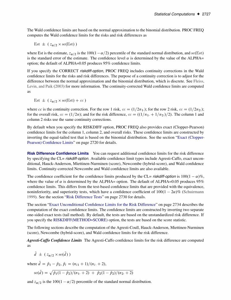
Statistical Computations F 2727
The Wald confidence limits are based on the normal approximation to the binomial distribution. PROC FREQcomputes the Wald confidence limits for the risks and risk differences as
Est ˙ . z˛=2 � se.Est/ /
where Est is the estimate, z˛=2 is the 100.1�˛=2/ percentile of the standard normal distribution, and se.Est/is the standard error of the estimate. The confidence level ˛ is determined by the value of the ALPHA=option; the default of ALPHA=0.05 produces 95% confidence limits.
If you specify the CORRECT riskdiff-option, PROC FREQ includes continuity corrections in the Waldconfidence limits for the risks and risk differences. The purpose of a continuity correction is to adjust for thedifference between the normal approximation and the binomial distribution, which is discrete. See Fleiss,Levin, and Paik (2003) for more information. The continuity-corrected Wald confidence limits are computedas
Est ˙ . z˛=2 � se.Est/C cc /
where cc is the continuity correction. For the row 1 risk, cc D .1=2n1�/; for the row 2 risk, cc D .1=2n2�/;for the overall risk, cc D .1=2n/; and for the risk difference, cc D ..1=n1� C 1=n2�/=2/. The column 1 andcolumn 2 risks use the same continuity corrections.
By default when you specify the RISKDIFF option, PROC FREQ also provides exact (Clopper-Pearson)confidence limits for the column 1, column 2, and overall risks. These confidence limits are constructed byinverting the equal-tailed test that is based on the binomial distribution. See the section “Exact (Clopper-Pearson) Confidence Limits” on page 2720 for details.
Risk Difference Confidence Limits You can request additional confidence limits for the risk differenceby specifying the CL= riskdiff-option. Available confidence limit types include Agresti-Caffo, exact uncon-ditional, Hauck-Anderson, Miettinen-Nurminen (score), Newcombe (hybrid-score), and Wald confidencelimits. Continuity-corrected Newcombe and Wald confidence limits are also available.
The confidence coefficient for the confidence limits produced by the CL= riskdiff-option is 100.1 � ˛/%,where the value of ˛ is determined by the ALPHA= option. The default of ALPHA=0.05 produces 95%confidence limits. This differs from the test-based confidence limits that are provided with the equivalence,noninferiority, and superiority tests, which have a confidence coefficient of 100.1 � 2˛/% (Schuirmann1999). See the section “Risk Difference Tests” on page 2730 for details.
The section “Exact Unconditional Confidence Limits for the Risk Difference” on page 2734 describes thecomputation of the exact confidence limits. The confidence limits are constructed by inverting two separateone-sided exact tests (tail method). By default, the tests are based on the unstandardized risk difference. Ifyou specify the RISKDIFF(METHOD=SCORE) option, the tests are based on the score statistic.
The following sections describe the computation of the Agresti-Coull, Hauck-Anderson, Miettinen-Nurminen(score), Newcombe (hybrid-score), and Wald confidence limits for the risk difference.
Agresti-Caffo Confidence Limits The Agresti-Caffo confidence limits for the risk difference are computedas
Qd ˙ . z˛=2 � se. Qd/ /
where Qd D Qp1 � Qp2, Qpi D .ni1 C 1/=.ni � C 2/,
se. Qd/ DpQp1.1 � Qp2/=.n1� C 2/ C Qp2.1 � Qp2/=.n2� C 2/
and z˛=2 is the 100.1 � ˛=2/ percentile of the standard normal distribution.

2728 F Chapter 40: The FREQ Procedure
The Agresti-Caffo interval adjusts the Wald interval for the risk difference by adding a pseudo-observation ofeach type (success and failure) to each sample. See Agresti and Caffo (2000) and Agresti and Coull (1998)for more information.
Hauck-Anderson Confidence Limits The Hauck-Anderson confidence limits for the risk difference arecomputed as
Od ˙ . cc C z˛=2 � se. Od/ /
where Od D Op1� Op2 and z˛=2 is the 100.1�˛=2/ percentile of the standard normal distribution. The standarderror is computed from the sample proportions as
se. Od/ DpOp1.1 � Op1/=.n1� � 1/ C Op2.1 � Op2/=.n2� � 1/
The Hauck-Anderson continuity correction cc is computed as
cc D 1 =�2 min.n1�; n2�/
�See Hauck and Anderson (1986) for more information. The subsection “Hauck-Anderson Test” in the section“Noninferiority Tests” on page 2731 describes the corresponding noninferiority test.
Miettinen-Nurminen (Score) Confidence Limits The Miettinen-Nurminen (score) confidence limits for therisk difference (Miettinen and Nurminen 1985) are computed by inverting score tests for the risk difference.A score-based test statistic for the null hypothesis that the risk difference equals ı can be expressed as
T .ı/ D . Od � ı/=
qeVar.ı/
where Od is the observed value of the risk difference ( Op1 � Op2),
eVar.ı/ D .n=.n � 1// . Qp1.ı/.1 � Qp1.ı//=n1 C Qp2.ı/.1 � Qp2.ı//=n2 /
and Qp1.ı/ and Qp2.ı/ are the maximum likelihood estimates of the row 1 and row 2 risks (proportions) underthe restriction that the risk difference is ı. For more information, see Miettinen and Nurminen (1985, pp.215–216) and Miettinen (1985, chapter 12).
The 100.1 � ˛/% confidence interval for the risk difference consists of all values of ı for which the scoretest statistic T .ı/ falls in the acceptance region,
fı W T .ı/ < z˛=2g
where z˛=2 is the 100.1 � ˛=2/ percentile of the standard normal distribution. PROC FREQ finds the confi-dence limits by iterative computation, which stops when the iteration increment falls below the convergencecriterion or when the maximum number of iterations is reached, whichever occurs first. By default, theconvergence criterion is 0.00000001 and the maximum number of iterations is 100.
By default, the Miettinen-Nurminen confidence limits include the bias correction factor n=.n � 1/ in thecomputation of eVar.ı/ (Miettinen and Nurminen 1985, p. 216). For more information, see Newcombe andNurminen (2011). If you specify the CL=MN(CORRECT=NO) riskdiff-option, PROC FREQ does not includethe bias correction factor in this computation (Mee 1984). See also Agresti (2002, p. 77). The uncorrectedconfidence limits are labeled as “Miettinen-Nurminen-Mee” confidence limits in the displayed output.

Statistical Computations F 2729
The maximum likelihood estimates of p1 and p2, subject to the constraint that the risk difference is ı, arecomputed as
Qp1 D 2u cos.w/ � b=3a and Qp2 D Qp1 C ı
where
w D .� C cos�1.v=u3//=3v D b3=.3a/3 � bc=6a2 C d=2a
u D sign.v/qb2=.3a/2 � c=3a
a D 1C �
b D � .1C � C Op1 C � Op2 C ı.� C 2//
c D ı2 C ı.2 Op1 C � C 1/C Op1 C � Op2
d D � Op1ı.1C ı/
� D n2�=n1�
For more information, see Farrington and Manning (1990, p. 1453).
Newcombe Confidence Limits Newcombe (hybrid-score) confidence limits for the risk difference areconstructed from the Wilson score confidence limits for each of the two individual proportions. Theconfidence limits for the individual proportions are used in the standard error terms of the Wald confidencelimits for the proportion difference. See Newcombe (1998a) and Barker et al. (2001) for more information.
Wilson score confidence limits for p1 and p2 are the roots of
jpi � Opi j D z˛=2ppi .1 � pi /=ni �
for i D 1; 2. The confidence limits are computed as�Opi C z2˛=2=2ni � ˙ z˛=2
q�Opi .1 � Opi /C z2˛=4ni �
�=ni �
�=�1C z2˛=2=ni �
�See the section “Wilson (Score) Confidence Limits” on page 2720 for details.
Denote the lower and upper Wilson score confidence limits for p1 as L1 and U1, and denote the lower andupper confidence limits for p2 as L2 and U2. The Newcombe confidence limits for the proportion difference(d D p1 � p2) are computed as
dL D . Op1 � Op2/ �
q. Op1 � L1/2 C .U2 � Op2/2
dU D . Op1 � Op2/ C
q.U1 � Op1/2 C . Op2 � L2/2
If you specify the CORRECT riskdiff-option, PROC FREQ provides continuity-corrected Newcombe con-fidence limits. By including a continuity correction of 1=2ni �, the Wilson score confidence limits for theindividual proportions are computed as the roots of
jpi � Opi j � 1=2ni � D z˛=2ppi .1 � pi /=ni �
The continuity-corrected confidence limits for the individual proportions are then used to compute theproportion difference confidence limits dL and dU .

2730 F Chapter 40: The FREQ Procedure
Wald Confidence Limits The Wald confidence limits for the risk difference are computed asOd ˙ . z˛=2 � se. Od/ /
where Od D Op1� Op2, z˛=2 is the 100.1�˛=2/ percentile of the standard normal distribution. and the standarderror is computed from the sample proportions as
se. Od/ DpOp1.1 � Op1/=n1� C Op2.1 � Op2/=n2�
If you specify the CORRECT riskdiff-option, the Wald confidence limits include a continuity correction cc,Od ˙ . cc C z˛=2 � se. Od/ /
where cc D .1=n1� C 1=n2�/=2.
The subsection “Wald Test” in the section “Noninferiority Tests” on page 2731 describes the correspondingnoninferiority test.
Risk Difference TestsYou can specify riskdiff-options to request tests of the risk (proportion) difference. You can request tests ofequality, noninferiority, superiority, and equivalence for the risk difference. The test of equality is a standardWald asymptotic test, available with or without a continuity correction. For noninferiority, superiority, andequivalence tests of the risk difference, the following test methods are provided: Wald (with and withoutcontinuity correction), Hauck-Anderson, Farrington-Manning (score), and Newcombe (with and withoutcontinuity correction). You can specify the test method with the METHOD= riskdiff-option. By default,PROC FREQ uses METHOD=WALD.
Equality Test If you specify the EQUAL riskdiff-option, PROC FREQ computes a test of equality, or a testof the null hypothesis that the risk difference equals zero. For the column 1 (or 2) risk difference, this test canbe expressed as H0W d D 0 versus the alternative HaW d ¤ 0, where d D p1 � p2 denotes the column 1 (or2) risk difference. PROC FREQ provides a Wald asymptotic test of equality. The test statistic is computed as
z D Od=se. Od/
By default, the standard error is computed from the sample proportions as
se. Od/ DpOp1.1 � Op1/=n1� C Op2.1 � Op2/=n2�
If you specify the VAR=NULL riskdiff-option, the standard error is based on the null hypothesis that the row1 and row 2 risks are equal,
se. Od/ DpOp.1 � Op/ � .1=n1� C 1=n2�/
where Op D n�1=n estimates the overall column 1 risk.
If you specify the CORRECT riskdiff-option, PROC FREQ includes a continuity correction in the test statistic.If Od > 0, the continuity correction is subtracted from Od in the numerator of the test statistic; otherwise, thecontinuity correction is added to the numerator. The value of the continuity correction is .1=n1� C 1=n2�/=2.
PROC FREQ computes one-sided and two-sided p-values for this test. When the test statistic z is greater than0, PROC FREQ displays the right-sided p-value, which is the probability of a larger value occurring underthe null hypothesis. The one-sided p-value can be expressed as
P1 D
(Prob.Z > z/ if z > 0
Prob.Z < z/ if z � 0
where Z has a standard normal distribution. The two-sided p-value is computed as P2 D 2 � P1.
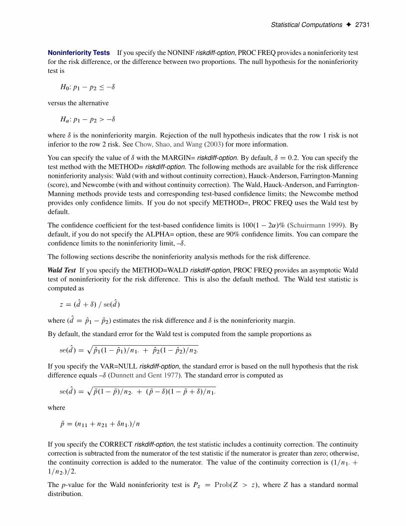
Statistical Computations F 2731
Noninferiority Tests If you specify the NONINF riskdiff-option, PROC FREQ provides a noninferiority testfor the risk difference, or the difference between two proportions. The null hypothesis for the noninferioritytest is
H0Wp1 � p2 � �ı
versus the alternative
HaWp1 � p2 > �ı
where ı is the noninferiority margin. Rejection of the null hypothesis indicates that the row 1 risk is notinferior to the row 2 risk. See Chow, Shao, and Wang (2003) for more information.
You can specify the value of ı with the MARGIN= riskdiff-option. By default, ı D 0:2. You can specify thetest method with the METHOD= riskdiff-option. The following methods are available for the risk differencenoninferiority analysis: Wald (with and without continuity correction), Hauck-Anderson, Farrington-Manning(score), and Newcombe (with and without continuity correction). The Wald, Hauck-Anderson, and Farrington-Manning methods provide tests and corresponding test-based confidence limits; the Newcombe methodprovides only confidence limits. If you do not specify METHOD=, PROC FREQ uses the Wald test bydefault.
The confidence coefficient for the test-based confidence limits is 100.1 � 2˛/% (Schuirmann 1999). Bydefault, if you do not specify the ALPHA= option, these are 90% confidence limits. You can compare theconfidence limits to the noninferiority limit, –ı.
The following sections describe the noninferiority analysis methods for the risk difference.
Wald Test If you specify the METHOD=WALD riskdiff-option, PROC FREQ provides an asymptotic Waldtest of noninferiority for the risk difference. This is also the default method. The Wald test statistic iscomputed as
z D . Od C ı/ = se. Od/
where ( Od D Op1 � Op2) estimates the risk difference and ı is the noninferiority margin.
By default, the standard error for the Wald test is computed from the sample proportions as
se. Od/ DpOp1.1 � Op1/=n1� C Op2.1 � Op2/=n2�
If you specify the VAR=NULL riskdiff-option, the standard error is based on the null hypothesis that the riskdifference equals –ı (Dunnett and Gent 1977). The standard error is computed as
se. Od/ DpQp.1 � Qp/=n2� C . Qp � ı/.1 � Qp C ı/=n1�
where
Qp D .n11 C n21 C ın1�/=n
If you specify the CORRECT riskdiff-option, the test statistic includes a continuity correction. The continuitycorrection is subtracted from the numerator of the test statistic if the numerator is greater than zero; otherwise,the continuity correction is added to the numerator. The value of the continuity correction is .1=n1� C1=n2�/=2.
The p-value for the Wald noninferiority test is Pz D Prob.Z > z/, where Z has a standard normaldistribution.

2732 F Chapter 40: The FREQ Procedure
Hauck-Anderson Test If you specify the METHOD=HA riskdiff-option, PROC FREQ provides the Hauck-Anderson test for noninferiority. The Hauck-Anderson test statistic is computed as
z D . Od C ı ˙ cc/ = se. Od/
where Od D Op1 � Op2 and the standard error is computed from the sample proportions as
se. Od/ DpOp1.1 � Op1/=.n1� � 1/ C Op2.1 � Op2/=.n2� � 1/
The Hauck-Anderson continuity correction cc is computed as
cc D 1 =�2 min.n1�; n2�/
�The p-value for the Hauck-Anderson noninferiority test is Pz D Prob.Z > z/, where Z has a standardnormal distribution. See Hauck and Anderson (1986) and Schuirmann (1999) for more information.
Farrington-Manning (Score) Test If you specify the METHOD=FM riskdiff-option, PROC FREQ providesthe Farrington-Manning (score) test of noninferiority for the risk difference. A score test statistic for the nullhypothesis that the risk difference equals –ı can be expressed as
z D . Od C ı/ = se. Od/
where Od is the observed value of the risk difference ( Op1 � Op2),
se. Od/ DpQp1.1 � Qp1/=n1� C Qp2.1 � Qp2/=n2�
and Qp1 and Qp2 are the maximum likelihood estimates of the row 1 and row 2 risks (proportions) under therestriction that the risk difference is –ı. The p-value for the noninferiority test is Pz D Prob.Z > z/, whereZ has a standard normal distribution. For more information, see Miettinen and Nurminen (1985); Miettinen(1985); Farrington and Manning (1990); Dann and Koch (2005).
The maximum likelihood estimates of p1 and p1, subject to the constraint that the risk difference is –ı, arecomputed as
Qp1 D 2u cos.w/ � b=3a and Qp2 D Qp1 C ı
where
w D .� C cos�1.v=u3//=3v D b3=.3a/3 � bc=6a2 C d=2a
u D sign.v/qb2=.3a/2 � c=3a
a D 1C �
b D � .1C � C Op1 C � Op2 � ı.� C 2//
c D ı2 � ı.2 Op1 C � C 1/C Op1 C � Op2
d D Op1ı.1 � ı/
� D n2�=n1�
For more information, see Farrington and Manning (1990, p. 1453).
Newcombe Noninferiority Analysis If you specify the METHOD=NEWCOMBE riskdiff-option, PROCFREQ provides a noninferiority analysis that is based on Newcombe hybrid-score confidence limits for the
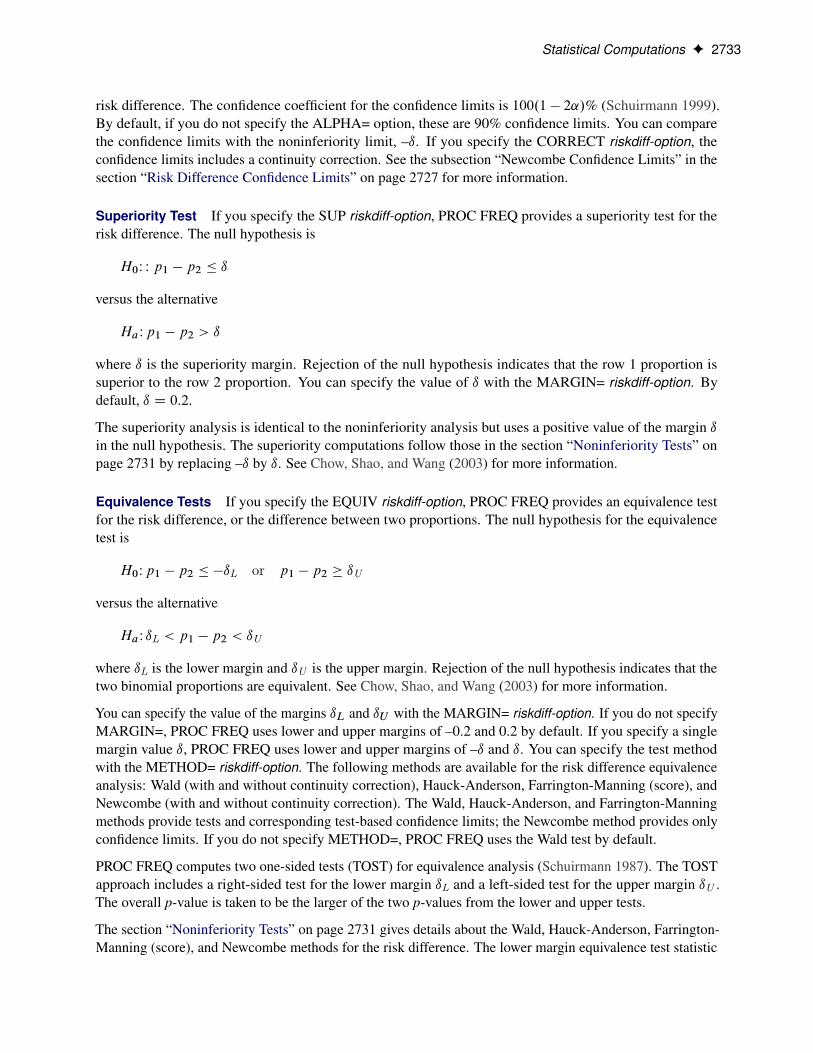
Statistical Computations F 2733
risk difference. The confidence coefficient for the confidence limits is 100.1 � 2˛/% (Schuirmann 1999).By default, if you do not specify the ALPHA= option, these are 90% confidence limits. You can comparethe confidence limits with the noninferiority limit, –ı. If you specify the CORRECT riskdiff-option, theconfidence limits includes a continuity correction. See the subsection “Newcombe Confidence Limits” in thesection “Risk Difference Confidence Limits” on page 2727 for more information.
Superiority Test If you specify the SUP riskdiff-option, PROC FREQ provides a superiority test for therisk difference. The null hypothesis is
H0W W p1 � p2 � ı
versus the alternative
HaWp1 � p2 > ı
where ı is the superiority margin. Rejection of the null hypothesis indicates that the row 1 proportion issuperior to the row 2 proportion. You can specify the value of ı with the MARGIN= riskdiff-option. Bydefault, ı D 0:2.
The superiority analysis is identical to the noninferiority analysis but uses a positive value of the margin ıin the null hypothesis. The superiority computations follow those in the section “Noninferiority Tests” onpage 2731 by replacing –ı by ı. See Chow, Shao, and Wang (2003) for more information.
Equivalence Tests If you specify the EQUIV riskdiff-option, PROC FREQ provides an equivalence testfor the risk difference, or the difference between two proportions. The null hypothesis for the equivalencetest is
H0Wp1 � p2 � �ıL or p1 � p2 � ıU
versus the alternative
HaW ıL < p1 � p2 < ıU
where ıL is the lower margin and ıU is the upper margin. Rejection of the null hypothesis indicates that thetwo binomial proportions are equivalent. See Chow, Shao, and Wang (2003) for more information.
You can specify the value of the margins ıL and ıU with the MARGIN= riskdiff-option. If you do not specifyMARGIN=, PROC FREQ uses lower and upper margins of –0.2 and 0.2 by default. If you specify a singlemargin value ı, PROC FREQ uses lower and upper margins of –ı and ı. You can specify the test methodwith the METHOD= riskdiff-option. The following methods are available for the risk difference equivalenceanalysis: Wald (with and without continuity correction), Hauck-Anderson, Farrington-Manning (score), andNewcombe (with and without continuity correction). The Wald, Hauck-Anderson, and Farrington-Manningmethods provide tests and corresponding test-based confidence limits; the Newcombe method provides onlyconfidence limits. If you do not specify METHOD=, PROC FREQ uses the Wald test by default.
PROC FREQ computes two one-sided tests (TOST) for equivalence analysis (Schuirmann 1987). The TOSTapproach includes a right-sided test for the lower margin ıL and a left-sided test for the upper margin ıU .The overall p-value is taken to be the larger of the two p-values from the lower and upper tests.
The section “Noninferiority Tests” on page 2731 gives details about the Wald, Hauck-Anderson, Farrington-Manning (score), and Newcombe methods for the risk difference. The lower margin equivalence test statistic
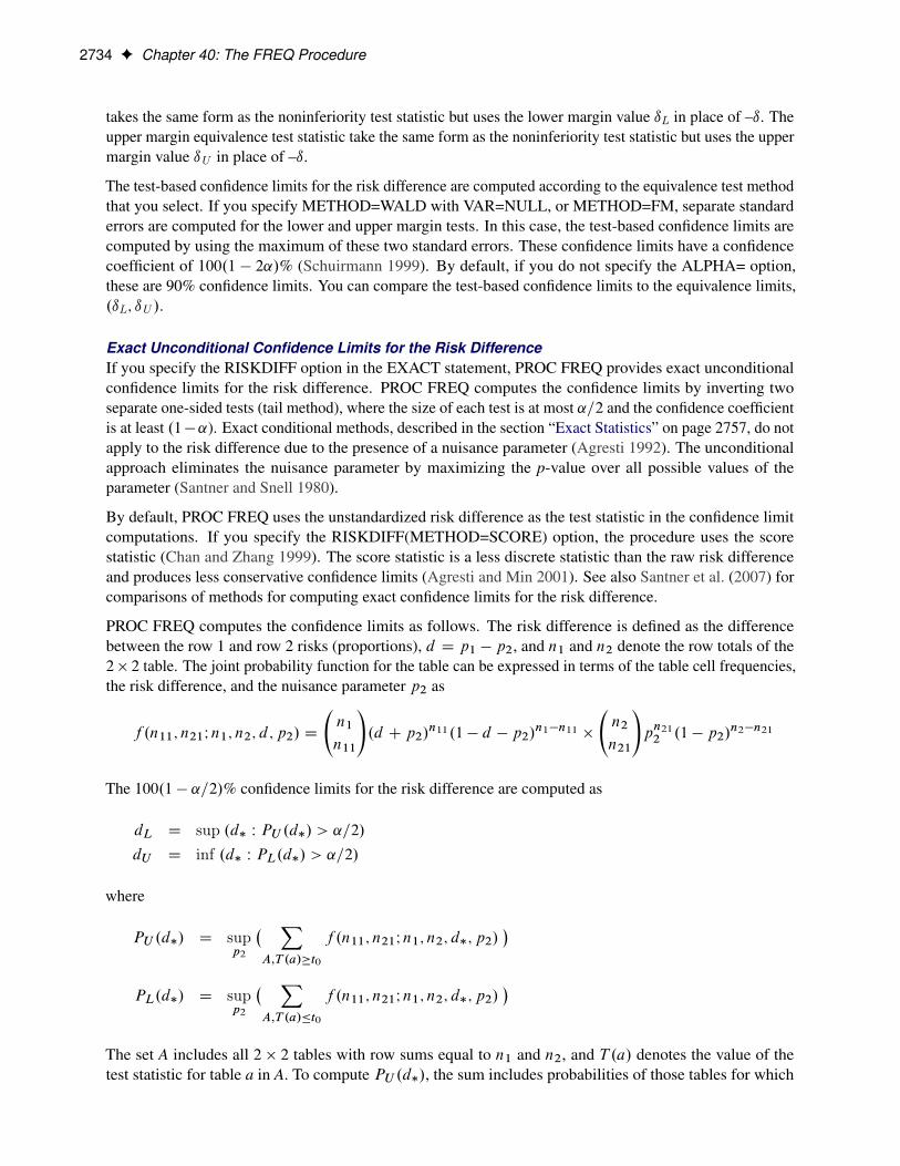
2734 F Chapter 40: The FREQ Procedure
takes the same form as the noninferiority test statistic but uses the lower margin value ıL in place of –ı. Theupper margin equivalence test statistic take the same form as the noninferiority test statistic but uses the uppermargin value ıU in place of –ı.
The test-based confidence limits for the risk difference are computed according to the equivalence test methodthat you select. If you specify METHOD=WALD with VAR=NULL, or METHOD=FM, separate standarderrors are computed for the lower and upper margin tests. In this case, the test-based confidence limits arecomputed by using the maximum of these two standard errors. These confidence limits have a confidencecoefficient of 100.1 � 2˛/% (Schuirmann 1999). By default, if you do not specify the ALPHA= option,these are 90% confidence limits. You can compare the test-based confidence limits to the equivalence limits,.ıL; ıU /.
Exact Unconditional Confidence Limits for the Risk DifferenceIf you specify the RISKDIFF option in the EXACT statement, PROC FREQ provides exact unconditionalconfidence limits for the risk difference. PROC FREQ computes the confidence limits by inverting twoseparate one-sided tests (tail method), where the size of each test is at most ˛=2 and the confidence coefficientis at least .1�˛). Exact conditional methods, described in the section “Exact Statistics” on page 2757, do notapply to the risk difference due to the presence of a nuisance parameter (Agresti 1992). The unconditionalapproach eliminates the nuisance parameter by maximizing the p-value over all possible values of theparameter (Santner and Snell 1980).
By default, PROC FREQ uses the unstandardized risk difference as the test statistic in the confidence limitcomputations. If you specify the RISKDIFF(METHOD=SCORE) option, the procedure uses the scorestatistic (Chan and Zhang 1999). The score statistic is a less discrete statistic than the raw risk differenceand produces less conservative confidence limits (Agresti and Min 2001). See also Santner et al. (2007) forcomparisons of methods for computing exact confidence limits for the risk difference.
PROC FREQ computes the confidence limits as follows. The risk difference is defined as the differencebetween the row 1 and row 2 risks (proportions), d D p1 � p2, and n1 and n2 denote the row totals of the2� 2 table. The joint probability function for the table can be expressed in terms of the table cell frequencies,the risk difference, and the nuisance parameter p2 as
f .n11; n21In1; n2; d; p2/ D
n1
n11
!.d C p2/
n11.1 � d � p2/n1�n11 �
n2
n21
!pn21
2 .1 � p2/n2�n21
The 100.1 � ˛=2/% confidence limits for the risk difference are computed as
dL D sup .d� W PU .d�/ > ˛=2/dU D inf .d� W PL.d�/ > ˛=2/
where
PU .d�/ D supp2
� XA;T .a/�t0
f .n11; n21In1; n2; d�; p2/�
PL.d�/ D supp2
� XA;T .a/�t0
f .n11; n21In1; n2; d�; p2/�
The set A includes all 2 � 2 tables with row sums equal to n1 and n2, and T .a/ denotes the value of thetest statistic for table a in A. To compute PU .d�/, the sum includes probabilities of those tables for which
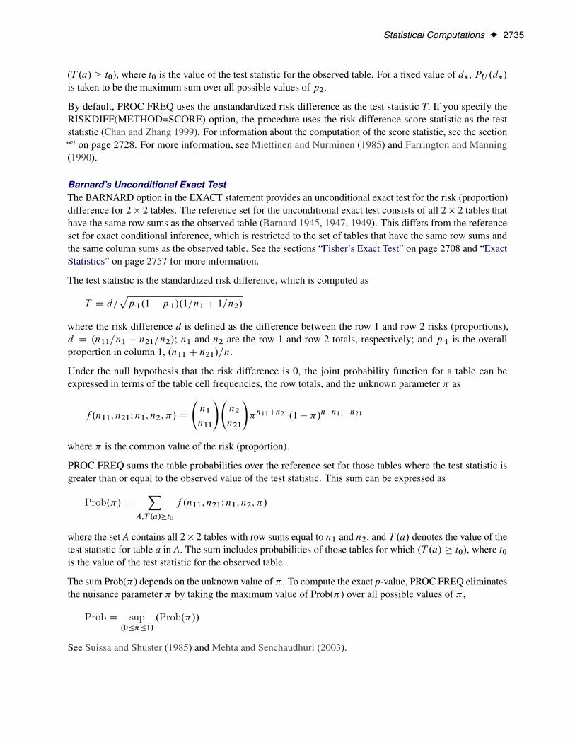
Statistical Computations F 2735
(T .a/ � t0), where t0 is the value of the test statistic for the observed table. For a fixed value of d�, PU .d�/is taken to be the maximum sum over all possible values of p2.
By default, PROC FREQ uses the unstandardized risk difference as the test statistic T. If you specify theRISKDIFF(METHOD=SCORE) option, the procedure uses the risk difference score statistic as the teststatistic (Chan and Zhang 1999). For information about the computation of the score statistic, see the section“” on page 2728. For more information, see Miettinen and Nurminen (1985) and Farrington and Manning(1990).
Barnard’s Unconditional Exact TestThe BARNARD option in the EXACT statement provides an unconditional exact test for the risk (proportion)difference for 2 � 2 tables. The reference set for the unconditional exact test consists of all 2 � 2 tables thathave the same row sums as the observed table (Barnard 1945, 1947, 1949). This differs from the referenceset for exact conditional inference, which is restricted to the set of tables that have the same row sums andthe same column sums as the observed table. See the sections “Fisher’s Exact Test” on page 2708 and “ExactStatistics” on page 2757 for more information.
The test statistic is the standardized risk difference, which is computed as
T D d=pp�1.1 � p�1/.1=n1 C 1=n2/
where the risk difference d is defined as the difference between the row 1 and row 2 risks (proportions),d D .n11=n1 � n21=n2/; n1 and n2 are the row 1 and row 2 totals, respectively; and p�1 is the overallproportion in column 1, .n11 C n21/=n.
Under the null hypothesis that the risk difference is 0, the joint probability function for a table can beexpressed in terms of the table cell frequencies, the row totals, and the unknown parameter � as
f .n11; n21In1; n2; �/ D
n1
n11
! n2
n21
!�n11Cn21.1 � �/n�n11�n21
where � is the common value of the risk (proportion).
PROC FREQ sums the table probabilities over the reference set for those tables where the test statistic isgreater than or equal to the observed value of the test statistic. This sum can be expressed as
Prob.�/ DX
A;T .a/�t0
f .n11; n21In1; n2; �/
where the set A contains all 2� 2 tables with row sums equal to n1 and n2, and T .a/ denotes the value of thetest statistic for table a in A. The sum includes probabilities of those tables for which (T .a/ � t0), where t0is the value of the test statistic for the observed table.
The sum Prob(�) depends on the unknown value of � . To compute the exact p-value, PROC FREQ eliminatesthe nuisance parameter � by taking the maximum value of Prob(�) over all possible values of � ,
Prob D sup.0���1/
.Prob.�//
See Suissa and Shuster (1985) and Mehta and Senchaudhuri (2003).
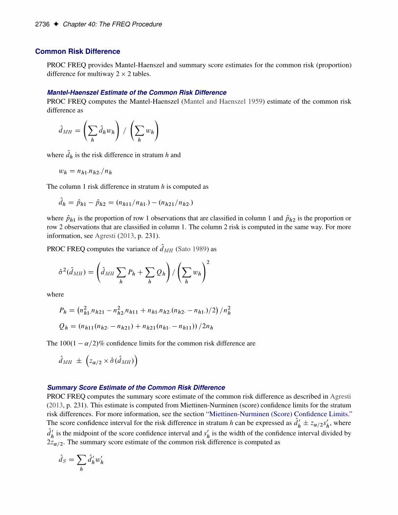
2736 F Chapter 40: The FREQ Procedure
Common Risk Difference
PROC FREQ provides Mantel-Haenszel and summary score estimates for the common risk (proportion)difference for multiway 2 � 2 tables.
Mantel-Haenszel Estimate of the Common Risk DifferencePROC FREQ computes the Mantel-Haenszel (Mantel and Haenszel 1959) estimate of the common riskdifference as
OdMH D
Xh
Odhwh
!=
Xh
wh
!
where Odh is the risk difference in stratum h and
wh D nh1�nh2�=nh
The column 1 risk difference in stratum h is computed as
Odh D Oph1 � Oph2 D .nh11=nh1�/ � .nh21=nh2�/
where Oph1 is the proportion of row 1 observations that are classified in column 1 and Oph2 is the proportion orrow 2 observations that are classified in column 1. The column 2 risk is computed in the same way. For moreinformation, see Agresti (2013, p. 231).
PROC FREQ computes the variance of OdMH (Sato 1989) as
O�2. OdMH / D
OdMH
Xh
Ph CXh
Qh
!=
Xh
wh
!2where
Ph D�n2h1�nh21 � n
2h2�nh11 C nh1�nh2�.nh2� � nh1�/=2
�=n2h
Qh D .nh11.nh2� � nh21/C nh21.nh1� � nh11// =2nh
The 100.1 � ˛=2/% confidence limits for the common risk difference are
OdMH ˙�z˛=2 � O�. OdMH /
�
Summary Score Estimate of the Common Risk DifferencePROC FREQ computes the summary score estimate of the common risk difference as described in Agresti(2013, p. 231). This estimate is computed from Miettinen-Nurminen (score) confidence limits for the stratumrisk differences. For more information, see the section “Miettinen-Nurminen (Score) Confidence Limits.”The score confidence interval for the risk difference in stratum h can be expressed as Od 0
h˙ z˛=2s
0h, where
Od 0h
is the midpoint of the score confidence interval and s0h
is the width of the confidence interval divided by2z˛=2. The summary score estimate of the common risk difference is computed as
OdS DXh
Od 0hw0h
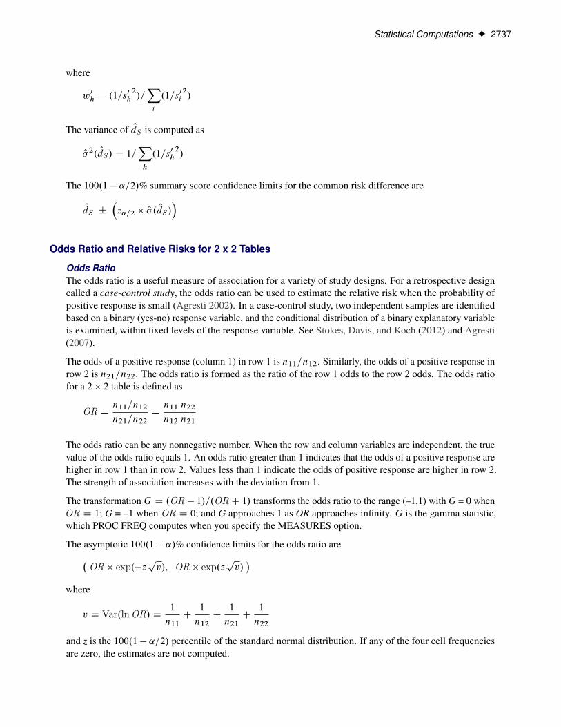
Statistical Computations F 2737
where
w0h D .1=s0h2/=Xi
.1=s0i2/
The variance of OdS is computed as
O�2. OdS / D 1=Xh
.1=s0h2/
The 100.1 � ˛=2/% summary score confidence limits for the common risk difference are
OdS ˙�z˛=2 � O�. OdS /
�
Odds Ratio and Relative Risks for 2 x 2 Tables
Odds RatioThe odds ratio is a useful measure of association for a variety of study designs. For a retrospective designcalled a case-control study, the odds ratio can be used to estimate the relative risk when the probability ofpositive response is small (Agresti 2002). In a case-control study, two independent samples are identifiedbased on a binary (yes-no) response variable, and the conditional distribution of a binary explanatory variableis examined, within fixed levels of the response variable. See Stokes, Davis, and Koch (2012) and Agresti(2007).
The odds of a positive response (column 1) in row 1 is n11=n12. Similarly, the odds of a positive response inrow 2 is n21=n22. The odds ratio is formed as the ratio of the row 1 odds to the row 2 odds. The odds ratiofor a 2 � 2 table is defined as
OR Dn11=n12
n21=n22Dn11 n22
n12 n21
The odds ratio can be any nonnegative number. When the row and column variables are independent, the truevalue of the odds ratio equals 1. An odds ratio greater than 1 indicates that the odds of a positive response arehigher in row 1 than in row 2. Values less than 1 indicate the odds of positive response are higher in row 2.The strength of association increases with the deviation from 1.
The transformation G D .OR � 1/=.OR C 1/ transforms the odds ratio to the range (–1,1) with G = 0 whenOR D 1; G = –1 when OR D 0; and G approaches 1 as OR approaches infinity. G is the gamma statistic,which PROC FREQ computes when you specify the MEASURES option.
The asymptotic 100.1 � ˛/% confidence limits for the odds ratio are�OR � exp.�z
pv/; OR � exp.z
pv/�
where
v D Var.lnOR/ D1
n11C
1
n12C
1
n21C
1
n22
and z is the 100.1 � ˛=2/ percentile of the standard normal distribution. If any of the four cell frequenciesare zero, the estimates are not computed.
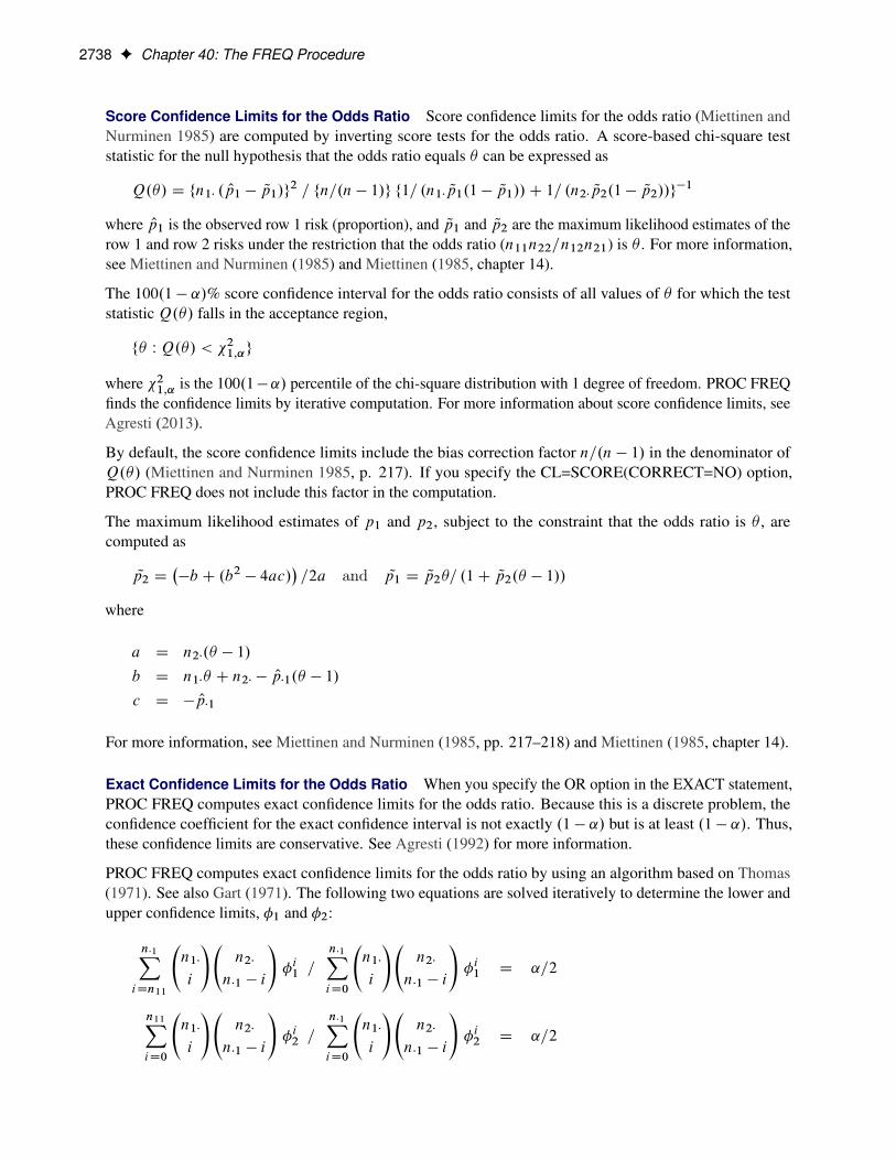
2738 F Chapter 40: The FREQ Procedure
Score Confidence Limits for the Odds Ratio Score confidence limits for the odds ratio (Miettinen andNurminen 1985) are computed by inverting score tests for the odds ratio. A score-based chi-square teststatistic for the null hypothesis that the odds ratio equals � can be expressed as
Q.�/ D fn1� . Op1 � Qp1/g2 = fn=.n � 1/g f1= .n1� Qp1.1 � Qp1//C 1= .n2� Qp2.1 � Qp2//g
�1
where Op1 is the observed row 1 risk (proportion), and Qp1 and Qp2 are the maximum likelihood estimates of therow 1 and row 2 risks under the restriction that the odds ratio (n11n22=n12n21) is � . For more information,see Miettinen and Nurminen (1985) and Miettinen (1985, chapter 14).
The 100.1 � ˛/% score confidence interval for the odds ratio consists of all values of � for which the teststatistic Q.�/ falls in the acceptance region,
f� W Q.�/ < �21;˛g
where �21;˛ is the 100.1�˛/ percentile of the chi-square distribution with 1 degree of freedom. PROC FREQfinds the confidence limits by iterative computation. For more information about score confidence limits, seeAgresti (2013).
By default, the score confidence limits include the bias correction factor n=.n � 1/ in the denominator ofQ.�/ (Miettinen and Nurminen 1985, p. 217). If you specify the CL=SCORE(CORRECT=NO) option,PROC FREQ does not include this factor in the computation.
The maximum likelihood estimates of p1 and p2, subject to the constraint that the odds ratio is � , arecomputed as
Qp2 D��b C .b2 � 4ac/
�=2a and Qp1 D Qp2�= .1C Qp2.� � 1//
where
a D n2�.� � 1/
b D n1�� C n2� � Op�1.� � 1/
c D � Op�1
For more information, see Miettinen and Nurminen (1985, pp. 217–218) and Miettinen (1985, chapter 14).
Exact Confidence Limits for the Odds Ratio When you specify the OR option in the EXACT statement,PROC FREQ computes exact confidence limits for the odds ratio. Because this is a discrete problem, theconfidence coefficient for the exact confidence interval is not exactly .1 � ˛/ but is at least .1 � ˛/. Thus,these confidence limits are conservative. See Agresti (1992) for more information.
PROC FREQ computes exact confidence limits for the odds ratio by using an algorithm based on Thomas(1971). See also Gart (1971). The following two equations are solved iteratively to determine the lower andupper confidence limits, �1 and �2:
n�1XiDn11
n1�
i
! n2�
n�1 � i
!�i1 =
n�1XiD0
n1�
i
! n2�
n�1 � i
!�i1 D ˛=2
n11XiD0
n1�
i
! n2�
n�1 � i
!�i2 =
n�1XiD0
n1�
i
! n2�
n�1 � i
!�i2 D ˛=2
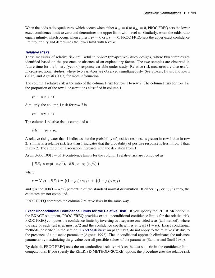
Statistical Computations F 2739
When the odds ratio equals zero, which occurs when either n11 D 0 or n22 D 0, PROC FREQ sets the lowerexact confidence limit to zero and determines the upper limit with level ˛. Similarly, when the odds ratioequals infinity, which occurs when either n12 D 0 or n21 D 0, PROC FREQ sets the upper exact confidencelimit to infinity and determines the lower limit with level ˛.
Relative RisksThese measures of relative risk are useful in cohort (prospective) study designs, where two samples areidentified based on the presence or absence of an explanatory factor. The two samples are observed infuture time for the binary (yes-no) response variable under study. Relative risk measures are also usefulin cross-sectional studies, where two variables are observed simultaneously. See Stokes, Davis, and Koch(2012) and Agresti (2007) for more information.
The column 1 relative risk is the ratio of the column 1 risk for row 1 to row 2. The column 1 risk for row 1 isthe proportion of the row 1 observations classified in column 1,
p1 D n11 = n1�
Similarly, the column 1 risk for row 2 is
p2 D n21 = n2�
The column 1 relative risk is computed as
RR1 D p1 = p2
A relative risk greater than 1 indicates that the probability of positive response is greater in row 1 than in row2. Similarly, a relative risk less than 1 indicates that the probability of positive response is less in row 1 thanin row 2. The strength of association increases with the deviation from 1.
Asymptotic 100.1 � ˛/% confidence limits for the column 1 relative risk are computed as�RR1 � exp.�z
pv/; RR1 � exp.z
pv/�
where
v D Var.lnRR1/ D�.1 � p1/=n11
�C�.1 � p2/=n21
�and z is the 100.1 � ˛=2/ percentile of the standard normal distribution. If either n11 or n21 is zero, theestimates are not computed.
PROC FREQ computes the column 2 relative risks in the same way.
Exact Unconditional Confidence Limits for the Relative Risk If you specify the RELRISK option inthe EXACT statement, PROC FREQ provides exact unconditional confidence limits for the relative risk.PROC FREQ computes the confidence limits by inverting two separate one-sided tests (tail method), wherethe size of each test is at most ˛=2 and the confidence coefficient is at least .1 � ˛/. Exact conditionalmethods, described in the section “Exact Statistics” on page 2757, do not apply to the relative risk due tothe presence of a nuisance parameter (Agresti 1992). The unconditional approach eliminates the nuisanceparameter by maximizing the p-value over all possible values of the parameter (Santner and Snell 1980).
By default, PROC FREQ uses the unstandardized relative risk as the test statistic in the confidence limitcomputations. If you specify the RELRISK(METHOD=SCORE) option, the procedure uses the relative risk

2740 F Chapter 40: The FREQ Procedure
score statistic (Chan and Zhang 1999). The score statistic is a less discrete statistic than the raw relative riskand produces less conservative confidence limits (Agresti and Min 2001). See also Santner et al. (2007) forcomparisons of methods for computing exact confidence limits.
See the section “Exact Unconditional Confidence Limits for the Risk Difference” on page 2734 for adescription of the method that PROC FREQ uses to compute confidence limits for the relative risk. Thetest statistic for the relative risk computation is either the unstandardized relative risk (by default) or therelative risk score statistic (if you specify the RELRISK(METHOD=SCORE) option). PROC FREQ usesthe following form of the unstandardized relative risk, which adds 0.05 to each frequency, to ensure that thestatistic is defined when there are zero table cells (Gart and Nam 1988):
rr D.n11 C 0:5/ = .n1� C 0:5/
.n21 C 0:5/ = .n2� C 0:5/
If you specify the RELRISK(METHOD=SCORE) option, PROC FREQ uses the relative risk score statistic(Miettinen and Nurminen 1985; Farrington and Manning 1990). This test statistic is computed as
z D . Op1 �R0 Op2/ = se.rr/
where
se.rr/ DqQp1.1 � Qp1/=n1� C R20 Qp2.1 � Qp2/=n2�
where Qp1 and Qp2 are the maximum likelihood estimators of p1 and p2 under the null hypothesis that therelative risk equals R0. From Farrington and Manning (1990, p. 1454), the maximum likelihood solution is
Qp1 D .�b �p
b2 � 4ac/=2a and Qp2 D Qp1=R0
where
a D 1C �
b D � .R0.1C � Op2/C � C Op1/
c D R0. Op1 C � Op2/
� D n2�=n1�
Cochran-Armitage Test for Trend
The TREND option in the TABLES statement provides the Cochran-Armitage test for trend, which testsfor trend in binomial proportions across levels of a single factor or covariate. This test is appropriate for atwo-way table where one variable has two levels and the other variable is ordinal. The two-level variablerepresents the response, and the other variable represents an explanatory variable with ordered levels. Whenthe two-way has two columns and R rows, PROC FREQ tests for trend across the R levels of the row variable,and the binomial proportion is computed as the proportion of observations in the first column. When thetable has two rows and C columns, PROC FREQ tests for trend across the C levels of the column variable,and the binomial proportion is computed as the proportion of observations in the first row.
The trend test is based on the regression coefficient for the weighted linear regression of the binomialproportions on the scores of the explanatory variable levels. See Margolin (1988) and Agresti (2002) fordetails. If the table has two columns and R rows, the trend test statistic is computed as
T D
RXiD1
ni1.Ri � NR/ =
qp�1 .1 � p�1/ s2

Statistical Computations F 2741
where Ri is the score of row i, NR is the average row score, and
s2 D
RXiD1
ni �.Ri � NR/2
The SCORES= option in the TABLES statement determines the type of row scores used in computing thetrend test (and other score-based statistics). The default is SCORES=TABLE. See the section “Scores” onpage 2703 for details. For character variables, the table scores for the row variable are the row numbers (forexample, 1 for the first row, 2 for the second row, and so on). For numeric variables, the table score for eachrow is the numeric value of the row level. When you perform the trend test, the explanatory variable mightbe numeric (for example, dose of a test substance), and the variable values might be appropriate scores. If theexplanatory variable has ordinal levels that are not numeric, you can assign meaningful scores to the variablelevels. Sometimes equidistant scores, such as the table scores for a character variable, might be appropriate.For more information on choosing scores for the trend test, see Margolin (1988).
The null hypothesis for the Cochran-Armitage test is no trend, which means that the binomial proportionpi1 D ni1=ni � is the same for all levels of the explanatory variable. Under the null hypothesis, the trendstatistic has an asymptotic standard normal distribution.
PROC FREQ computes one-sided and two-sided p-values for the trend test. When the test statistic is greaterthan its null hypothesis expected value of zero, PROC FREQ displays the right-sided p-value, which is theprobability of a larger value of the statistic occurring under the null hypothesis. A small right-sided p-valuesupports the alternative hypothesis of increasing trend in proportions from row 1 to row R. When the teststatistic is less than or equal to zero, PROC FREQ displays the left-sided p-value. A small left-sided p-valuesupports the alternative of decreasing trend.
The one-sided p-value for the trend test is computed as
P1 D
(Prob.Z > T / if T > 0
Prob.Z < T / if T � 0
where Z has a standard normal distribution. The two-sided p-value is computed as
P2 D Prob.jZj > jT j/
PROC FREQ also provides exact p-values for the Cochran-Armitage trend test. You can request the exact testby specifying the TREND option in the EXACT statement. See the section “Exact Statistics” on page 2757for more information.
Jonckheere-Terpstra Test
The JT option in the TABLES statement provides the Jonckheere-Terpstra test, which is a nonparametrictest for ordered differences among classes. It tests the null hypothesis that the distribution of the responsevariable does not differ among classes. It is designed to detect alternatives of ordered class differences, whichcan be expressed as �1 � �2 � � � � � �R (or �1 � �2 � � � � � �R), with at least one of the inequalities beingstrict, where �i denotes the effect of class i. For such ordered alternatives, the Jonckheere-Terpstra test can bepreferable to tests of more general class difference alternatives, such as the Kruskal–Wallis test (produced bythe WILCOXON option in the NPAR1WAY procedure). See Pirie (1983) and Hollander and Wolfe (1999)for more information about the Jonckheere-Terpstra test.
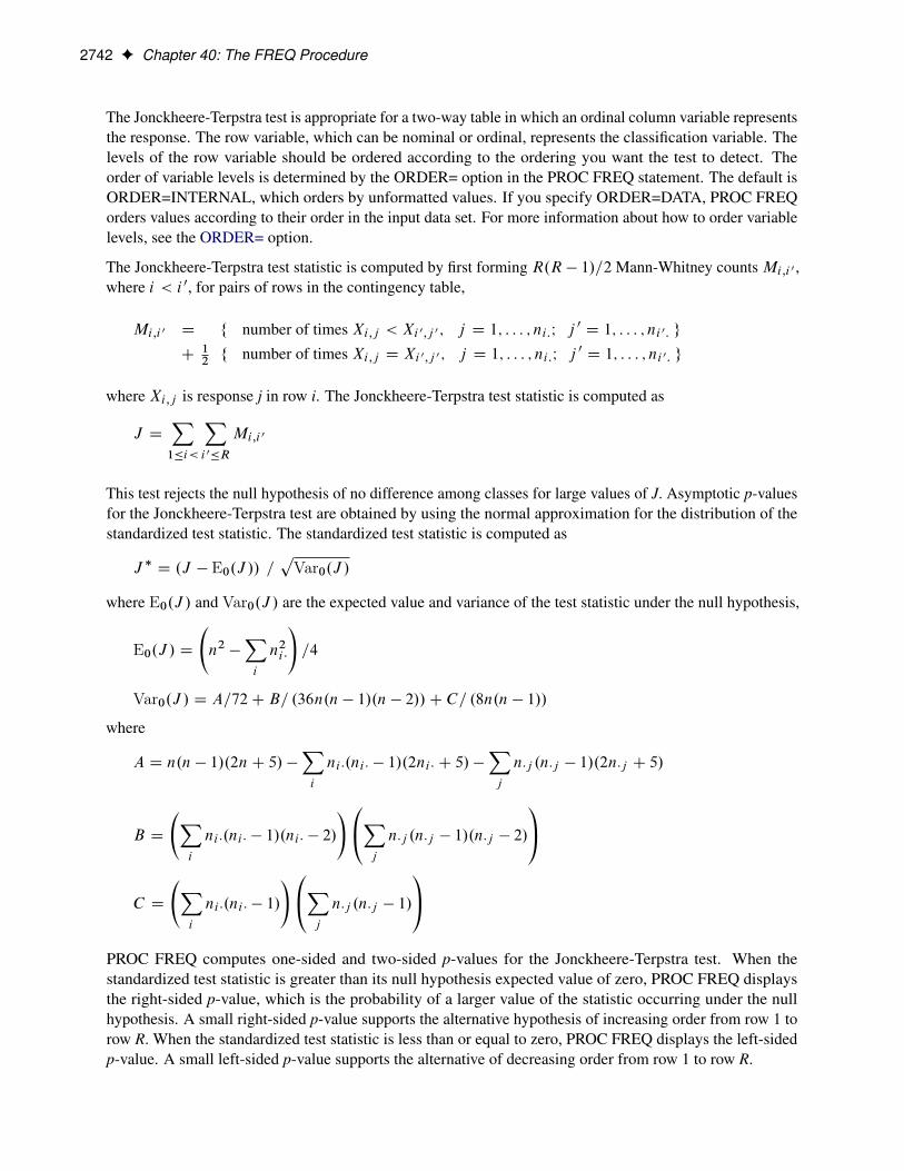
2742 F Chapter 40: The FREQ Procedure
The Jonckheere-Terpstra test is appropriate for a two-way table in which an ordinal column variable representsthe response. The row variable, which can be nominal or ordinal, represents the classification variable. Thelevels of the row variable should be ordered according to the ordering you want the test to detect. Theorder of variable levels is determined by the ORDER= option in the PROC FREQ statement. The default isORDER=INTERNAL, which orders by unformatted values. If you specify ORDER=DATA, PROC FREQorders values according to their order in the input data set. For more information about how to order variablelevels, see the ORDER= option.
The Jonckheere-Terpstra test statistic is computed by first forming R.R � 1/=2 Mann-Whitney counts Mi;i 0 ,where i < i 0, for pairs of rows in the contingency table,
Mi;i 0 D f number of times Xi;j < Xi 0;j 0 ; j D 1; : : : ; ni:I j0D 1; : : : ; ni 0: g
C12f number of times Xi;j D Xi 0;j 0 ; j D 1; : : : ; ni:I j
0D 1; : : : ; ni 0: g
where Xi;j is response j in row i. The Jonckheere-Terpstra test statistic is computed as
J DX1�i<
Xi 0�R
Mi;i 0
This test rejects the null hypothesis of no difference among classes for large values of J. Asymptotic p-valuesfor the Jonckheere-Terpstra test are obtained by using the normal approximation for the distribution of thestandardized test statistic. The standardized test statistic is computed as
J � D .J � E0.J // =p
Var0.J /
where E0.J / and Var0.J / are the expected value and variance of the test statistic under the null hypothesis,
E0.J / D
n2 �
Xi
n2i �
!=4
Var0.J / D A=72C B= .36n.n � 1/.n � 2//C C= .8n.n � 1//
where
A D n.n � 1/.2nC 5/ �Xi
ni �.ni � � 1/.2ni � C 5/ �Xj
n�j .n�j � 1/.2n�j C 5/
B D
Xi
ni �.ni � � 1/.ni � � 2/
!0@Xj
n�j .n�j � 1/.n�j � 2/
1AC D
Xi
ni �.ni � � 1/
!0@Xj
n�j .n�j � 1/
1APROC FREQ computes one-sided and two-sided p-values for the Jonckheere-Terpstra test. When thestandardized test statistic is greater than its null hypothesis expected value of zero, PROC FREQ displaysthe right-sided p-value, which is the probability of a larger value of the statistic occurring under the nullhypothesis. A small right-sided p-value supports the alternative hypothesis of increasing order from row 1 torow R. When the standardized test statistic is less than or equal to zero, PROC FREQ displays the left-sidedp-value. A small left-sided p-value supports the alternative of decreasing order from row 1 to row R.
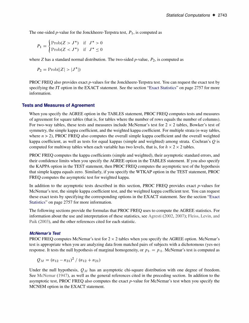
Statistical Computations F 2743
The one-sided p-value for the Jonckheere-Terpstra test, P1, is computed as
P1 D
(Prob.Z > J �/ if J � > 0
Prob.Z < J �/ if J � � 0
where Z has a standard normal distribution. The two-sided p-value, P2, is computed as
P2 D Prob.jZj > jJ �j/
PROC FREQ also provides exact p-values for the Jonckheere-Terpstra test. You can request the exact test byspecifying the JT option in the EXACT statement. See the section “Exact Statistics” on page 2757 for moreinformation.
Tests and Measures of Agreement
When you specify the AGREE option in the TABLES statement, PROC FREQ computes tests and measuresof agreement for square tables (that is, for tables where the number of rows equals the number of columns).For two-way tables, these tests and measures include McNemar’s test for 2 � 2 tables, Bowker’s test ofsymmetry, the simple kappa coefficient, and the weighted kappa coefficient. For multiple strata (n-way tables,where n > 2), PROC FREQ also computes the overall simple kappa coefficient and the overall weightedkappa coefficient, as well as tests for equal kappas (simple and weighted) among strata. Cochran’s Q iscomputed for multiway tables when each variable has two levels, that is, for h � 2 � 2 tables.
PROC FREQ computes the kappa coefficients (simple and weighted), their asymptotic standard errors, andtheir confidence limits when you specify the AGREE option in the TABLES statement. If you also specifythe KAPPA option in the TEST statement, then PROC FREQ computes the asymptotic test of the hypothesisthat simple kappa equals zero. Similarly, if you specify the WTKAP option in the TEST statement, PROCFREQ computes the asymptotic test for weighted kappa.
In addition to the asymptotic tests described in this section, PROC FREQ provides exact p-values forMcNemar’s test, the simple kappa coefficient test, and the weighted kappa coefficient test. You can requestthese exact tests by specifying the corresponding options in the EXACT statement. See the section “ExactStatistics” on page 2757 for more information.
The following sections provide the formulas that PROC FREQ uses to compute the AGREE statistics. Forinformation about the use and interpretation of these statistics, see Agresti (2002, 2007); Fleiss, Levin, andPaik (2003), and the other references cited for each statistic.
McNemar’s TestPROC FREQ computes McNemar’s test for 2 � 2 tables when you specify the AGREE option. McNemar’stest is appropriate when you are analyzing data from matched pairs of subjects with a dichotomous (yes-no)response. It tests the null hypothesis of marginal homogeneity, or p1� D p�1. McNemar’s test is computed as
QM D .n12 � n21/2 = .n12 C n21/
Under the null hypothesis, QM has an asymptotic chi-square distribution with one degree of freedom.See McNemar (1947), as well as the general references cited in the preceding section. In addition to theasymptotic test, PROC FREQ also computes the exact p-value for McNemar’s test when you specify theMCNEM option in the EXACT statement.
2744 F Chapter 40: The FREQ Procedure
Bowker’s Test of SymmetryFor Bowker’s test of symmetry, the null hypothesis is that the cell proportions are symmetric, or thatpij D pj i for all pairs of table cells. For 2 � 2 tables, Bowker’s test is identical to McNemar’s test, and soPROC FREQ provides Bowker’s test for square tables larger than 2 � 2.
Bowker’s test of symmetry is computed as
QB D
XXi<j
.nij � nj i /2 = .nij C nj i /
For large samples, QB has an asymptotic chi-square distribution with R.R � 1/=2 degrees of freedom underthe null hypothesis of symmetry. See Bowker (1948) for details.
Simple Kappa CoefficientThe simple kappa coefficient, introduced by Cohen (1960), is a measure of interrater agreement. PROCFREQ computes the simple kappa coefficient as
O� D .Po � Pe/ = .1 � Pe/
where Po DPi pi i and Pe D
Pi pi:p:i . If the two response variables are viewed as two independent
ratings of the n subjects, the kappa coefficient equals +1 when there is complete agreement of the raters.When the observed agreement exceeds chance agreement, kappa is positive, with its magnitude reflecting thestrength of agreement. Although this is unusual in practice, kappa is negative when the observed agreementis less than chance agreement. The minimum value of kappa is between –1 and 0, depending on the marginalproportions.
The asymptotic variance of the simple kappa coefficient is computed as
Var. O�/ D .AC B � C/ = .1 � Pe/2 n
where
A D
Xi
pi i .1 � .pi � C p�i /.1 � O�//2
B D .1 � O�/2XXi¤j
pij .p�i C pj �/2
C D . O� � Pe.1 � O�/ /2
See Fleiss, Cohen, and Everitt (1969) for details.
PROC FREQ computes confidence limits for the simple kappa coefficient as
O� ˙�z˛=2 �
pVar. O�/
�where z˛=2 is the 100.1 � ˛=2/ percentile of the standard normal distribution. The value of ˛ is determinedby the value of the ALPHA= option, which, by default, equals 0.05 and produces 95% confidence limits.
To compute an asymptotic test for the kappa coefficient, PROC FREQ uses the standardized test statistic O��,which has an asymptotic standard normal distribution under the null hypothesis that kappa equals zero. Thestandardized test statistic is computed as
O�� D O� =p
Var0. O�/

Statistical Computations F 2745
where Var0. O�/ is the variance of the kappa coefficient under the null hypothesis,
Var0. O�/ D
Pe C P
2e �
Xi
pi �p�i .pi � C p�i /
!= .1 � Pe/
2 n
See Fleiss, Levin, and Paik (2003) for details.
PROC FREQ also provides an exact test for the simple kappa coefficient. You can request the exact test byspecifying the KAPPA or AGREE option in the EXACT statement. See the section “Exact Statistics” onpage 2757 for more information.
Weighted Kappa CoefficientThe weighted kappa coefficient is a generalization of the simple kappa coefficient that uses weights toquantify the relative difference between categories. For 2 � 2 tables, the weighted kappa coefficient equalsthe simple kappa coefficient. PROC FREQ displays the weighted kappa coefficient only for tables larger than2 � 2. PROC FREQ computes the kappa weights from the column scores, by using either Cicchetti-Allisonweights or Fleiss-Cohen weights, both of which are described in the following section. The weights wijare constructed so that 0 � wij < 1 for all i 6D j , wi i D 1 for all i, and wij D wj i . The weighted kappacoefficient is computed as
O�w D�Po.w/ � Pe.w/
�=�1 � Pe.w/
�where
Po.w/ DXi
Xj
wijpij
Pe.w/ DXi
Xj
wijpi �p�j
The asymptotic variance of the weighted kappa coefficient is
Var. O�w/ D
0@Xi
Xj
pij�wij � .wi � C w�j /.1 � O�w/
�2��O�w � Pe.w/.1 � O�w/
�21A = .1�Pe.w//2 n
where
wi � DXj
p�jwij
w�j DXi
pi �wij
See Fleiss, Cohen, and Everitt (1969) for details.
PROC FREQ computes confidence limits for the weighted kappa coefficient as
O�w ˙�z˛=2 �
pVar. O�w/
�where z˛=2 is the 100.1 � ˛=2/ percentile of the standard normal distribution. The value of ˛ is determinedby the value of the ALPHA= option, which, by default, equals 0.05 and produces 95% confidence limits.

2746 F Chapter 40: The FREQ Procedure
To compute an asymptotic test for the weighted kappa coefficient, PROC FREQ uses the standardized teststatistic O��w , which has an asymptotic standard normal distribution under the null hypothesis that weightedkappa equals zero. The standardized test statistic is computed as
O��w D O�w =p
Var0. O�w/
where Var0. O�w/ is the variance of the weighted kappa coefficient under the null hypothesis,
Var0. O�w/ D
0@Xi
Xj
pi �p�j�wij � .wi � C w�j /
�2� P 2e.w/
1A = .1 � Pe.w//2 n
See Fleiss, Levin, and Paik (2003) for details.
PROC FREQ also provides an exact test for the weighted kappa coefficient. You can request the exact test byspecifying the WTKAPPA or AGREE option in the EXACT statement. See the section “Exact Statistics” onpage 2757 for more information.
Weights PROC FREQ computes kappa coefficient weights by using the column scores and one of thetwo available weight types. The column scores are determined by the SCORES= option in the TABLESstatement. The two available types of kappa weights are Cicchetti-Allison and Fleiss-Cohen weights. Bydefault, PROC FREQ uses Cicchetti-Allison weights. If you specify (WT=FC) with the AGREE option, thenPROC FREQ uses Fleiss-Cohen weights to compute the weighted kappa coefficient.
PROC FREQ computes Cicchetti-Allison kappa coefficient weights as
wij D 1 �jCi � Cj j
CC � C1
where Ci is the score for column i and C is the number of categories or columns. See Cicchetti and Allison(1971) for details.
The SCORES= option in the TABLES statement determines the type of column scores used to compute thekappa weights (and other score-based statistics). The default is SCORES=TABLE. See the section “Scores”on page 2703 for details. For numeric variables, table scores are the values of the variable levels. You canassign numeric values to the levels in a way that reflects their level of similarity. For example, suppose youhave four levels and order them according to similarity. If you assign them values of 0, 2, 4, and 10, theCicchetti-Allison kappa weights take the following values: w12 = 0.8, w13 = 0.6, w14 = 0, w23 = 0.8, w24= 0.2, and w34 = 0.4. Note that when there are only two categories (that is, C = 2), the weighted kappacoefficient is identical to the simple kappa coefficient.
If you specify (WT=FC) with the AGREE option in the TABLES statement, PROC FREQ computesFleiss-Cohen kappa coefficient weights as
wij D 1 �.Ci � Cj /
2
.CC � C1/2
See Fleiss and Cohen (1973) for details.
For the preceding example, the Fleiss-Cohen kappa weights are: w12 = 0.96, w13 = 0.84, w14 = 0, w23 =0.96, w24 = 0.36, and w34 = 0.64.

Statistical Computations F 2747
Overall Kappa CoefficientWhen there are multiple strata, PROC FREQ combines the stratum-level estimates of kappa into an overallestimate of the supposed common value of kappa. Assume there are q strata, indexed by h D 1; 2; : : : ; q,and let Var. O�h/ denote the variance of O�h. The estimate of the overall kappa coefficient is computed as
O�T D
qXhD1
O�h
Var. O�h/=
qXhD1
1
Var. O�h/
See Fleiss, Levin, and Paik (2003) for details.
PROC FREQ computes an estimate of the overall weighted kappa in the same way.
Tests for Equal Kappa CoefficientsWhen there are multiple strata, the following chi-square statistic tests whether the stratum-level values ofkappa are equal:
QK D
qXhD1
. O�h � O�T /2 = Var. O�h/
Under the null hypothesis of equal kappas for the q strata, QK has an asymptotic chi-square distribution withq–1 degrees of freedom. See Fleiss, Levin, and Paik (2003) for more information. PROC FREQ computes atest for equal weighted kappa coefficients in the same way.
Cochran’s Q TestCochran’s Q is computed for multiway tables when each variable has two levels, that is, for 2 � 2 � � � � 2tables. Cochran’s Q statistic is used to test the homogeneity of the one-dimensional margins. Let m denotethe number of variables and N denote the total number of subjects. Cochran’s Q statistic is computed as
QC D m.m � 1/
0@ mXjD1
T 2j � T2
1A =
mT �
NXkD1
S2k
!
where Tj is the number of positive responses for variable j, T is the total number of positive responses overall variables, and Sk is the number of positive responses for subject k. Under the null hypothesis, Cochran’sQ has an asymptotic chi-square distribution with m–1 degrees of freedom. See Cochran (1950) for details.When there are only two binary response variables (m=2), Cochran’s Q simplifies to McNemar’s test. Whenthere are more than two response categories, you can test for marginal homogeneity by using the repeatedmeasures capabilities of the CATMOD procedure.
Tables with Zero Rows and ColumnsThe AGREE statistics are defined only for square tables, where the number of rows equals the number ofcolumns. If the table is not square, PROC FREQ does not compute AGREE statistics. In the kappa statisticframework, where two independent raters assign ratings to each of n subjects, suppose one of the ratersdoes not use all possible r rating levels. If the corresponding table has r rows but only r–1 columns, thenthe table is not square and PROC FREQ does not compute AGREE statistics. To create a square table inthis situation, use the ZEROS option in the WEIGHT statement, which requests that PROC FREQ includeobservations with zero weights in the analysis. Include zero-weight observations in the input data set to

2748 F Chapter 40: The FREQ Procedure
represent any rating levels that are not used by a rater, so that the input data set has at least one observationfor each possible rater and rating combination. The analysis then includes all rating levels, even when alllevels are not actually assigned by both raters. The resulting table (of rater 1 by rater 2) is a square table, andAGREE statistics can be computed.
For more information, see the description of the ZEROS option. By default, PROC FREQ does not processobservations that have zero weights, because these observations do not contribute to the total frequency count,and because any resulting zero-weight row or column causes many of the tests and measures of associationto be undefined. However, kappa statistics are defined for tables with a zero-weight row or column, andthe ZEROS option makes it possible to input zero-weight observations and construct the tables needed tocompute kappas.
Cochran-Mantel-Haenszel Statistics
The CMH option in the TABLES statement gives a stratified statistical analysis of the relationship betweenthe row and column variables after controlling for the strata variables in a multiway table. For example, forthe table request A*B*C*D, the CMH option provides an analysis of the relationship between C and D, aftercontrolling for A and B. The stratified analysis provides a way to adjust for the possible confounding effectsof A and B without being forced to estimate parameters for them.
The CMH analysis produces Cochran-Mantel-Haenszel statistics, which include the correlation statistic, theANOVA (row mean scores) statistic, and the general association statistic. For 2 � 2 tables, the CMH optionalso provides Mantel-Haenszel and logit estimates of the common odds ratio and the common relative risks,as well as the Breslow-Day test for homogeneity of the odds ratios.
Exact statistics are also available for stratified 2 � 2 tables. If you specify the EQOR option in the EXACTstatement, PROC FREQ provides Zelen’s exact test for equal odds ratios. If you specify the COMOR optionin the EXACT statement, PROC FREQ provides exact confidence limits for the common odds ratio and anexact test that the common odds ratio equals one.
Let the number of strata be denoted by q, indexing the strata by h D 1; 2; : : : ; q. Each stratum contains acontingency table with X representing the row variable and Y representing the column variable. For table h,denote the cell frequency in row i and column j by nhij , with corresponding row and column marginal totalsdenoted by nhi: and nh:j , and the overall stratum total by nh.
Because the formulas for the Cochran-Mantel-Haenszel statistics are more easily defined in terms of matrices,the following notation is used. Vectors are presumed to be column vectors unless they are transposed .0/.
n0hi
D .nhi1; nhi2; : : : ; nhiC / .1 � C/
n0h
D .n0h1; n0h2; : : : ; n0
hR/ .1 �RC/
phi � D nhi � = nh .1 � 1/
ph�j D nh�j = nh .1 � 1/
P0h��D .ph1�; ph2�; : : : ; phR�/ .1 �R/
P0h��D .ph�1; ph�2; : : : ; ph�C / .1 � C/
Assume that the strata are independent and that the marginal totals of each stratum are fixed. The nullhypothesis, H0, is that there is no association between X and Y in any of the strata. The corresponding model
Statistical Computations F 2749
is the multiple hypergeometric; this implies that, under H0, the expected value and covariance matrix of thefrequencies are, respectively,
mh D EŒnh jH0� D nh.Ph�� ˝ Ph��/
VarŒnh jH0� D c�.DPh�� � Ph��P0h��/˝ .DPh�� � Ph��P0h��/
�where
c D n2h = .nh � 1/
and where˝ denotes Kronecker product multiplication and Da is a diagonal matrix with the elements of aon the main diagonal.
The generalized CMH statistic (Landis, Heyman, and Koch 1978) is defined as
QCMH D G0VG�1G
where
G D
Xh
Bh.nh �mh/
VG D
Xh
Bh .VarŒnh jH0�/B0h
and where
Bh D Ch ˝Rh
is a matrix of fixed constants based on column scores Ch and row scores Rh. When the null hypothesis istrue, the CMH statistic has an asymptotic chi-square distribution with degrees of freedom equal to the rank ofBh. If VG is found to be singular, PROC FREQ prints a message and sets the value of the CMH statistic tomissing.
PROC FREQ computes three CMH statistics by using this formula for the generalized CMH statistic, withdifferent row and column score definitions for each statistic. The CMH statistics that PROC FREQ computesare the correlation statistic, the ANOVA (row mean scores) statistic, and the general association statistic.These statistics test the null hypothesis of no association against different alternative hypotheses. Thefollowing sections describe the computation of these CMH statistics.
CAUTION: The CMH statistics have low power for detecting an association in which the patterns ofassociation for some of the strata are in the opposite direction of the patterns displayed by other strata. Thus,a nonsignificant CMH statistic suggests either that there is no association or that no pattern of association hasenough strength or consistency to dominate any other pattern.
Correlation StatisticThe correlation statistic, popularized by Mantel and Haenszel, has one degree of freedom and is known as theMantel-Haenszel statistic (Mantel and Haenszel 1959; Mantel 1963).
The alternative hypothesis for the correlation statistic is that there is a linear association between X and Y inat least one stratum. If either X or Y does not lie on an ordinal (or interval) scale, then this statistic is notmeaningful.

2750 F Chapter 40: The FREQ Procedure
To compute the correlation statistic, PROC FREQ uses the formula for the generalized CMH statistic withthe row and column scores determined by the SCORES= option in the TABLES statement. See the section“Scores” on page 2703 for more information about the available score types. The matrix of row scores Rhhas dimension 1 �R, and the matrix of column scores Ch has dimension 1 � C .
When there is only one stratum, this CMH statistic reduces to .n � 1/r2, where r is the Pearson correlationcoefficient between X and Y. When nonparametric (RANK or RIDIT) scores are specified, the statisticreduces to .n � 1/r2s , where rs is the Spearman rank correlation coefficient between X and Y. When there ismore than one stratum, this CMH statistic becomes a stratum-adjusted correlation statistic.
ANOVA (Row Mean Scores) StatisticThe ANOVA statistic can be used only when the column variable Y lies on an ordinal (or interval) scale sothat the mean score of Y is meaningful. For the ANOVA statistic, the mean score is computed for each row ofthe table, and the alternative hypothesis is that, for at least one stratum, the mean scores of the R rows areunequal. In other words, the statistic is sensitive to location differences among the R distributions of Y.
The matrix of column scores Ch has dimension 1�C , and the column scores are determined by the SCORES=option.
The matrix of row scores Rh has dimension .R � 1/ �R and is created internally by PROC FREQ as
Rh D ŒIR�1;�JR�1�
where IR�1 is an identity matrix of rank R – 1 and JR�1 is an .R � 1/ � 1 vector of ones. This matrix hasthe effect of forming R – 1 independent contrasts of the R mean scores.
When there is only one stratum, this CMH statistic is essentially an analysis of variance (ANOVA) statistic inthe sense that it is a function of the variance ratio F statistic that would be obtained from a one-way ANOVAon the dependent variable Y. If nonparametric scores are specified in this case, then the ANOVA statistic is aKruskal-Wallis test.
If there is more than one stratum, then this CMH statistic corresponds to a stratum-adjusted ANOVA orKruskal-Wallis test. In the special case where there is one subject per row and one subject per column in thecontingency table of each stratum, this CMH statistic is identical to Friedman’s chi-square. See Example 40.9for an illustration.
General Association StatisticThe alternative hypothesis for the general association statistic is that, for at least one stratum, there is somekind of association between X and Y. This statistic is always interpretable because it does not require anordinal scale for either X or Y.
For the general association statistic, the matrix Rh is the same as the one used for the ANOVA statistic. Thematrix Ch is defined similarly as
Ch D ŒIC�1;�JC�1�
PROC FREQ generates both score matrices internally. When there is only one stratum, then the generalassociation CMH statistic reduces toQP .n�1/=n, whereQP is the Pearson chi-square statistic. When thereis more than one stratum, then the CMH statistic becomes a stratum-adjusted Pearson chi-square statistic.Note that a similar adjustment can be made by summing the Pearson chi-squares across the strata. However,

Statistical Computations F 2751
the latter statistic requires a large sample size in each stratum to support the resulting chi-square distributionwith q(R–1)(C–1) degrees of freedom. The CMH statistic requires only a large overall sample size because ithas only (R–1)(C–1) degrees of freedom.
See Cochran (1954); Mantel and Haenszel (1959); Mantel (1963); Birch (1965); Landis, Heyman, and Koch(1978).
Mantel-Fleiss CriterionIf you specify the CMH(MANTELFLEISS) option in the TABLES statement, PROC FREQ computes theMantel-Fleiss criterion for stratified 2 � 2 tables. The Mantel-Fleiss criterion can be used to assess thevalidity of the chi-square approximation for the distribution of the Mantel-Haenszel statistic for 2 � 2 tables.For details, see Mantel and Fleiss (1980); Mantel and Haenszel (1959); Stokes, Davis, and Koch (2012);Dmitrienko et al. (2005).
The Mantel-Fleiss criterion is computed as
MF D min
"Xh
mh11 �Xh
.nh11/L
#;
"Xh
.nh11/U �Xh
mh11
# !
wheremh11 is the expected value of nh11 under the hypothesis of no association between the row and columnvariables in table h, .nh11/L is the minimum possible value of the table cell frequency, and .nh11/U is themaximum possible value,
mh11 D nh1� nh�1 = nh
.nh11/L D max . 0; nh1� � nh�2 /
.nh11/U D min . nh�1; nh1� /
The Mantel-Fleiss guideline accepts the validity of the Mantel-Haenszel approximation when the value of thecriterion is at least 5. When the criterion is less than 5, PROC FREQ displays a warning.
Adjusted Odds Ratio and Relative Risk EstimatesThe CMH option provides adjusted odds ratio and relative risk estimates for stratified 2 � 2 tables. For eachof these measures, PROC FREQ computes a Mantel-Haenszel estimate and a logit estimate. These estimatesapply to n-way table requests in the TABLES statement, when the row and column variables both have twolevels.
For example, for the table request A*B*C*D, if the row and column variables C and D both have two levels,PROC FREQ provides odds ratio and relative risk estimates, adjusting for the confounding variables A and B.
The choice of an appropriate measure depends on the study design. For case-control (retrospective) studies,the odds ratio is appropriate. For cohort (prospective) or cross-sectional studies, the relative risk is appropriate.See the section “Odds Ratio and Relative Risks for 2 x 2 Tables” on page 2737 for more information on thesemeasures.
Throughout this section, z denotes the 100.1 � ˛=2/ percentile of the standard normal distribution.
2752 F Chapter 40: The FREQ Procedure
Odds Ratio, Case-Control Studies PROC FREQ provides Mantel-Haenszel and logit estimates for thecommon odds ratio for stratified 2 � 2 tables.
Mantel-Haenszel Estimator The Mantel-Haenszel estimate of the common odds ratio is computed as
ORMH D
Xh
nh11 nh22=nh
!=
Xh
nh12 nh21=nh
!
It is always computed unless the denominator is zero. See Mantel and Haenszel (1959) and Agresti (2002)for details.
To compute confidence limits for the common odds ratio, PROC FREQ uses the Robins, Breslow, andGreenland (1986) variance estimate for ln.ORMH /. The 100.1 � ˛=2/% confidence limits for the commonodds ratio are�
ORMH � exp.�z O�/; ORMH � exp.z O�/�
where
O�2 D bVar. ln.ORMH / /
D
Ph.nh11 C nh22/.nh11 nh22/=n
2h
2�P
h nh11 nh22=nh�2
C
PhŒ.nh11 C nh22/.nh12 nh21/C .nh12 C nh21/.nh11 nh22/�=n
2h
2�P
h nh11 nh22=nh� �P
h nh12 nh21=nh�
C
Ph.nh12 C nh21/.nh12 nh21/=n
2h
2�P
h nh12 nh21=nh�2
Note that the Mantel-Haenszel odds ratio estimator is less sensitive to small nh than the logit estimator.
Logit Estimator The adjusted logit estimate of the common odds ratio (Woolf 1955) is computed as
ORL D exp
Xh
wh ln.ORh/ =Xh
wh
!
and the corresponding 100.1 � ˛/% confidence limits are0@ ORL � exp
0@�z=sXh
wh
1A ; ORL � exp
0@z=sXh
wh
1A 1Awhere ORh is the odds ratio for stratum h, and
wh D 1=Var.ln.ORh//
If any table cell frequency in a stratum h is zero, PROC FREQ adds 0.5 to each cell of the stratum beforecomputing ORh and wh (Haldane 1955) for the logit estimate. The procedure prints a warning when thisoccurs.
Statistical Computations F 2753
Relative Risks, Cohort Studies PROC FREQ provides Mantel-Haenszel and logit estimates of thecommon relative risks for stratified 2 � 2 tables.
Mantel-Haenszel Estimator The Mantel-Haenszel estimate of the common relative risk for column 1 iscomputed as
RRMH D
Xh
nh11 nh2� = nh
!=
Xh
nh21 nh1� = nh
!
It is always computed unless the denominator is zero. See Mantel and Haenszel (1959) and Agresti (2002)for more information.
To compute confidence limits for the common relative risk, PROC FREQ uses the Greenland and Robins(1985) variance estimate for log.RRMH /. The 100.1 � ˛=2/% confidence limits for the common relativerisk are�
RRMH � exp.�z O�/; RRMH � exp.z O�/�
where
O�2 DbVar. ln.RRMH / / D
Ph.nh1� nh2� nh�1 � nh11 nh21 nh/=n
2h�P
h nh11 nh2�=nh� �P
h nh21 nh1�=nh�
Logit Estimator The adjusted logit estimate of the common relative risk for column 1 is computed as
RRL D exp
Xh
wh ln.RRh/ =X
wh
!
and the corresponding 100.1 � ˛/% confidence limits are0@ RRL � exp
0@�z =sXh
wh
1A ; RRL � exp
0@z =sXh
wh
1A 1Awhere RRh is the column 1 relative risk estimate for stratum h and
wh D 1 = Var.ln.RRh//
If nh11 or nh21 is zero, then PROC FREQ adds 0.5 to each cell of the stratum before computing RRh andwh for the logit estimate. The procedure prints a warning when this occurs. See Kleinbaum, Kupper, andMorgenstern (1982, Sections 17.4 and 17.5) for details.
Breslow-Day Test for Homogeneity of the Odds RatiosWhen you specify the CMH option, PROC FREQ computes the Breslow-Day test for stratified 2 � 2 tables.It tests the null hypothesis that the odds ratios for the q strata are equal. When the null hypothesis is true,the statistic has approximately a chi-square distribution with q–1 degrees of freedom. See Breslow and Day(1980) and Agresti (2007) for more information.
The Breslow-Day statistic is computed as
QBD DXh
.nh11 � E.nh11 j ORMH //2 = Var.nh11 j ORMH /

2754 F Chapter 40: The FREQ Procedure
where E and Var denote expected value and variance, respectively. The summation does not include any tablewith a zero row or column. If ORMH equals zero or if it is undefined, then PROC FREQ does not computethe statistic and prints a warning message.
For the Breslow-Day test to be valid, the sample size should be relatively large in each stratum, and at least80% of the expected cell counts should be greater than 5. Note that this is a stricter sample size requirementthan the requirement for the Cochran-Mantel-Haenszel test for q � 2 � 2 tables, in that each stratum samplesize (not just the overall sample size) must be relatively large. Even when the Breslow-Day test is valid, itmight not be very powerful against certain alternatives, as discussed in Breslow and Day (1980).
If you specify the BDT option, PROC FREQ computes the Breslow-Day test with Tarone’s adjustment,which subtracts an adjustment factor from QBD to make the resulting statistic asymptotically chi-square.The Breslow-Day-Tarone statistic is computed as
QBDT D QBD �
Xh
.nh11 � E.nh11 j ORMH //
!2=Xh
Var.nh11 j ORMH /
See Tarone (1985); Jones et al. (1989); Breslow (1996) for more information.
Zelen’s Exact Test for Equal Odds RatiosIf you specify the EQOR option in the EXACT statement, PROC FREQ computes Zelen’s exact test for equalodds ratios for stratified 2 � 2 tables. Zelen’s test is an exact counterpart to the Breslow-Day asymptotic testfor equal odds ratios. The reference set for Zelen’s test includes all possible q�2�2 tables with the same row,column, and stratum totals as the observed multiway table and with the same sum of cell (1,1) frequencies asthe observed table. The test statistic is the probability of the observed q � 2� 2 table conditional on the fixedmargins, which is a product of hypergeometric probabilities.
The p-value for Zelen’s test is the sum of all table probabilities that are less than or equal to the observedtable probability, where the sum is computed over all tables in the reference set determined by the fixedmargins and the observed sum of cell (1,1) frequencies. This test is similar to Fisher’s exact test for two-waytables. For more information, see Zelen (1971); Hirji (2006); Agresti (1992). PROC FREQ computes Zelen’sexact test by using the polynomial multiplication algorithm of Hirji et al. (1996).
Exact Confidence Limits for the Common Odds RatioIf you specify the COMOR option in the EXACT statement, PROC FREQ computes exact confidence limitsfor the common odds ratio for stratified 2� 2 tables. This computation assumes that the odds ratio is constantover all the 2 � 2 tables. Exact confidence limits are constructed from the distribution of S D
Ph nh11,
conditional on the marginal totals of the 2 � 2 tables.
Because this is a discrete problem, the confidence coefficient for these exact confidence limits is not exactly.1 � ˛/ but is at least .1 � ˛/. Thus, these confidence limits are conservative. See Agresti (1992) for moreinformation.
PROC FREQ computes exact confidence limits for the common odds ratio by using an algorithm based onVollset, Hirji, and Elashoff (1991). See also Mehta, Patel, and Gray (1985).
Conditional on the marginal totals of 2 � 2 table h, let the random variable Sh denote the frequency of tablecell (1,1). Given the row totals nh1� and nh2� and column totals nh�1 and nh�2, the lower and upper bounds forSh are lh and uh,
lh D max . 0; nh1� � nh�2 /uh D min . nh1�; nh�1 /

Statistical Computations F 2755
Let Csh denote the hypergeometric coefficient,
Csh D
nh�1
sh
! nh�2
nh1� � sh
!
and let � denote the common odds ratio. Then the conditional distribution of Sh is
P. Sh D sh j n1�; n�1; n�2 / D Csh �sh =
x D uhXx D lh
Cx �x
Summing over all the 2 � 2 tables, S DPh Sh, and the lower and upper bounds of S are l and u,
l DXh
lh and u DXh
uh
The conditional distribution of the sum S is
P. S D s j nh1�; nh�1; nh�2I h D 1; : : : ; q / D Cs �s =
x D uXx D l
Cx �x
where
Cs DX
s1C::::Csq D s
Yh
Csh
!
Let s0 denote the observed sum of cell (1,1) frequencies over the q tables. The following two equations aresolved iteratively for lower and upper confidence limits for the common odds ratio, �1 and �2:
x D uXx D s0
Cx �x1 =
x D uXx D l
Cx �x1 D ˛=2
x D s0Xx D l
Cx �x2 =
x D uXx D l
Cx �x2 D ˛=2
When the observed sum s0 equals the lower bound l, PROC FREQ sets the lower confidence limit to zeroand determines the upper limit with level ˛. Similarly, when the observed sum s0 equals the upper bound u,PROC FREQ sets the upper confidence limit to infinity and determines the lower limit with level ˛.
When you specify the COMOR option in the EXACT statement, PROC FREQ also computes the exact testthat the common odds ratio equals one. Setting � D 1, the conditional distribution of the sum S under thenull hypothesis becomes
P0. S D s j nh1�; nh�1; nh�2I h D 1; : : : ; q / D Cs =
x D uXx D l
Cx

2756 F Chapter 40: The FREQ Procedure
The point probability for this exact test is the probability of the observed sum s0 under the null hypothesis,conditional on the marginals of the stratified 2 � 2 tables, and is denoted by P0.s0/. The expected value of Sunder the null hypothesis is
E0.S/ Dx D uXx D l
x Cx =
x D uXx D l
Cx
The one-sided exact p-value is computed from the conditional distribution as P0.S >D s0/ or P0.S � s0/,depending on whether the observed sum s0 is greater or less than E0.S/,
P1 D P0. S >D s0 / D
x D uXx D s0
Cx =
x D uXx D l
Cx if s0 > E0.S/
P1 D P0. S <D s0 / D
x D s0Xx D l
Cx =
x D uXx D l
Cx if s0 � E0.S/
PROC FREQ computes two-sided p-values for this test according to three different definitions. A two-sidedp-value is computed as twice the one-sided p-value, setting the result equal to one if it exceeds one,
P a2 D 2 � P1
Additionally, a two-sided p-value is computed as the sum of all probabilities less than or equal to the pointprobability of the observed sum s0, summing over all possible values of s, l � s � u,
P b2 D
Xl�s�uWP0.s/�P0.s0/
P0.s/
Also, a two-sided p-value is computed as the sum of the one-sided p-value and the corresponding area in theopposite tail of the distribution, equidistant from the expected value,
P c2 D P0 . jS � E0.S/j � js0 � E0.S/j /
Gail-Simon Test for Qualitative Interactions
The GAILSIMON option in the TABLES statement provides the Gail-Simon test for qualitative interactionfor stratified 2� 2 tables. For details, see Gail and Simon (1985); Silvapulle (2001); Dmitrienko et al. (2005).
The Gail-Simon test is based on the risk differences in stratified 2 � 2 tables, where the risk differenceis defined as the row 1 risk (proportion in column 1) minus the row 2 risk. See the section “Risks andRisk Differences” on page 2725 for details. By default, the procedure uses column 1 risks to compute theGail-Simon test. If you specify the GAILSIMON(COLUMN=2) option, the procedure uses column 2 risks.
PROC FREQ computes the Gail-Simon test statistics as described in Gail and Simon (1985),
Q� D
Xh
.dh=sh/2 I.dh > 0/
QC D
Xh
.dh=sh/2 I.dh < 0/
Q D min .Q�; QC/
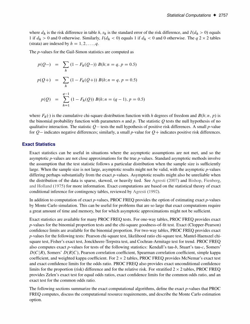
Statistical Computations F 2757
where dh is the risk difference in table h, sh is the standard error of the risk difference, and I.dh > 0/ equals1 if dh > 0 and 0 otherwise. Similarly, I.dh < 0/ equals 1 if dh < 0 and 0 otherwise. The q 2 � 2 tables(strata) are indexed by h D 1; 2; : : : ; q.
The p-values for the Gail-Simon statistics are computed as
p.Q�/ DXh
.1 � Fh.Q�// B.hIn D q; p D 0:5/
p.QC/ DXh
.1 � Fh.QC// B.hIn D q; p D 0:5/
p.Q/ D
q�1XhD1
.1 � Fh.Q// B.hIn D .q � 1/; p D 0:5/
where Fh.�/ is the cumulative chi-square distribution function with h degrees of freedom and B.hIn; p/ isthe binomial probability function with parameters n and p. The statistic Q tests the null hypothesis of noqualitative interaction. The statistic Q� tests the null hypothesis of positive risk differences. A small p-valuefor Q� indicates negative differences; similarly, a small p-value for QC indicates positive risk differences.
Exact Statistics
Exact statistics can be useful in situations where the asymptotic assumptions are not met, and so theasymptotic p-values are not close approximations for the true p-values. Standard asymptotic methods involvethe assumption that the test statistic follows a particular distribution when the sample size is sufficientlylarge. When the sample size is not large, asymptotic results might not be valid, with the asymptotic p-valuesdiffering perhaps substantially from the exact p-values. Asymptotic results might also be unreliable whenthe distribution of the data is sparse, skewed, or heavily tied. See Agresti (2007) and Bishop, Fienberg,and Holland (1975) for more information. Exact computations are based on the statistical theory of exactconditional inference for contingency tables, reviewed by Agresti (1992).
In addition to computation of exact p-values, PROC FREQ provides the option of estimating exact p-valuesby Monte Carlo simulation. This can be useful for problems that are so large that exact computations requirea great amount of time and memory, but for which asymptotic approximations might not be sufficient.
Exact statistics are available for many PROC FREQ tests. For one-way tables, PROC FREQ provides exactp-values for the binomial proportion tests and the chi-square goodness-of-fit test. Exact (Clopper-Pearson)confidence limits are available for the binomial proportion. For two-way tables, PROC FREQ provides exactp-values for the following tests: Pearson chi-square test, likelihood ratio chi-square test, Mantel-Haenszel chi-square test, Fisher’s exact test, Jonckheere-Terpstra test, and Cochran-Armitage test for trend. PROC FREQalso computes exact p-values for tests of the following statistics: Kendall’s tau-b, Stuart’s tau-c, Somers’D.C jR/, Somers’ D.RjC/, Pearson correlation coefficient, Spearman correlation coefficient, simple kappacoefficient, and weighted kappa coefficient. For 2 � 2 tables, PROC FREQ provides McNemar’s exact testand exact confidence limits for the odds ratio. PROC FREQ also provides exact unconditional confidencelimits for the proportion (risk) difference and for the relative risk. For stratified 2 � 2 tables, PROC FREQprovides Zelen’s exact test for equal odds ratios, exact confidence limits for the common odds ratio, and anexact test for the common odds ratio.
The following sections summarize the exact computational algorithms, define the exact p-values that PROCFREQ computes, discuss the computational resource requirements, and describe the Monte Carlo estimationoption.
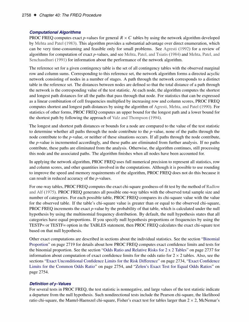
2758 F Chapter 40: The FREQ Procedure
Computational AlgorithmsPROC FREQ computes exact p-values for general R � C tables by using the network algorithm developedby Mehta and Patel (1983). This algorithm provides a substantial advantage over direct enumeration, whichcan be very time-consuming and feasible only for small problems. See Agresti (1992) for a review ofalgorithms for computation of exact p-values, and see Mehta, Patel, and Tsiatis (1984) and Mehta, Patel, andSenchaudhuri (1991) for information about the performance of the network algorithm.
The reference set for a given contingency table is the set of all contingency tables with the observed marginalrow and column sums. Corresponding to this reference set, the network algorithm forms a directed acyclicnetwork consisting of nodes in a number of stages. A path through the network corresponds to a distincttable in the reference set. The distances between nodes are defined so that the total distance of a path throughthe network is the corresponding value of the test statistic. At each node, the algorithm computes the shortestand longest path distances for all the paths that pass through that node. For statistics that can be expressedas a linear combination of cell frequencies multiplied by increasing row and column scores, PROC FREQcomputes shortest and longest path distances by using the algorithm of Agresti, Mehta, and Patel (1990). Forstatistics of other forms, PROC FREQ computes an upper bound for the longest path and a lower bound forthe shortest path by following the approach of Valz and Thompson (1994).
The longest and shortest path distances or bounds for a node are compared to the value of the test statisticto determine whether all paths through the node contribute to the p-value, none of the paths through thenode contribute to the p-value, or neither of these situations occurs. If all paths through the node contribute,the p-value is incremented accordingly, and these paths are eliminated from further analysis. If no pathscontribute, these paths are eliminated from the analysis. Otherwise, the algorithm continues, still processingthis node and the associated paths. The algorithm finishes when all nodes have been accounted for.
In applying the network algorithm, PROC FREQ uses full numerical precision to represent all statistics, rowand column scores, and other quantities involved in the computations. Although it is possible to use roundingto improve the speed and memory requirements of the algorithm, PROC FREQ does not do this because itcan result in reduced accuracy of the p-values.
For one-way tables, PROC FREQ computes the exact chi-square goodness-of-fit test by the method of Radlowand Alf (1975). PROC FREQ generates all possible one-way tables with the observed total sample size andnumber of categories. For each possible table, PROC FREQ compares its chi-square value with the valuefor the observed table. If the table’s chi-square value is greater than or equal to the observed chi-square,PROC FREQ increments the exact p-value by the probability of that table, which is calculated under the nullhypothesis by using the multinomial frequency distribution. By default, the null hypothesis states that allcategories have equal proportions. If you specify null hypothesis proportions or frequencies by using theTESTP= or TESTF= option in the TABLES statement, then PROC FREQ calculates the exact chi-square testbased on that null hypothesis.
Other exact computations are described in sections about the individual statistics. See the section “BinomialProportion” on page 2719 for details about how PROC FREQ computes exact confidence limits and tests forthe binomial proportion. See the section “Odds Ratio and Relative Risks for 2 x 2 Tables” on page 2737 forinformation about computation of exact confidence limits for the odds ratio for 2 � 2 tables. Also, see thesections “Exact Unconditional Confidence Limits for the Risk Difference” on page 2734, “Exact ConfidenceLimits for the Common Odds Ratio” on page 2754, and “Zelen’s Exact Test for Equal Odds Ratios” onpage 2754.
Definition of p-ValuesFor several tests in PROC FREQ, the test statistic is nonnegative, and large values of the test statistic indicatea departure from the null hypothesis. Such nondirectional tests include the Pearson chi-square, the likelihoodratio chi-square, the Mantel-Haenszel chi-square, Fisher’s exact test for tables larger than 2 � 2, McNemar’s

Statistical Computations F 2759
test, and the one-way chi-square goodness-of-fit test. The exact p-value for a nondirectional test is the sumof probabilities for those tables having a test statistic greater than or equal to the value of the observed teststatistic.
There are other tests where it might be appropriate to test against either a one-sided or a two-sided alternativehypothesis. For example, when you test the null hypothesis that the true parameter value equals 0 (T D 0),the alternative of interest might be one-sided (T � 0, or T � 0) or two-sided (T ¤ 0). Such tests include thePearson correlation coefficient, Spearman correlation coefficient, Jonckheere-Terpstra test, Cochran-Armitagetest for trend, simple kappa coefficient, and weighted kappa coefficient. For these tests, PROC FREQ displaysthe right-sided p-value when the observed value of the test statistic is greater than its expected value. Theright-sided p-value is the sum of probabilities for those tables for which the test statistic is greater than orequal to the observed test statistic. Otherwise, when the observed test statistic is less than or equal to theexpected value, PROC FREQ displays the left-sided p-value. The left-sided p-value is the sum of probabilitiesfor those tables for which the test statistic is less than or equal to the one observed. The one-sided p-value P1can be expressed as
P1 D
(Prob. Test Statistic � t / if t > E0.T /Prob. Test Statistic � t / if t � E0.T /
where t is the observed value of the test statistic and E0.T / is the expected value of the test statistic under thenull hypothesis. PROC FREQ computes the two-sided p-value as the sum of the one-sided p-value and thecorresponding area in the opposite tail of the distribution of the statistic, equidistant from the expected value.The two-sided p-value P2 can be expressed as
P2 D Prob . jTest Statistic � E0.T /j � jt � E0.T /j/
If you specify the POINT option in the EXACT statement, PROC FREQ provides exact point probabilities forthe exact tests. The exact point probability is the exact probability that the test statistic equals the observedvalue.
If you specify the MIDP option in the EXACT statement, PROC FREQ provides exact mid-p-values. Theexact mid p-value is defined as the exact p-value minus half the exact point probability, which equals theaverage of Prob.Test Statistic � t / and Prob.Test Statistic > t/ for a right-sided test. The exact mid p-valueis smaller and less conservative than the non-adjusted exact p-value. For more information, see Agresti (2013,section 1.1.4) and Hirji (2006, sections 2.5 and 2.11.1).
Computational ResourcesPROC FREQ uses relatively fast and efficient algorithms for exact computations. These recently developedalgorithms, together with improvements in computer power, now make it feasible to perform exact compu-tations for data sets where previously only asymptotic methods could be applied. Nevertheless, there arestill large problems that might require a prohibitive amount of time and memory for exact computations,depending on the speed and memory available on your computer. For large problems, consider whether exactmethods are really needed or whether asymptotic methods might give results quite close to the exact results,while requiring much less computer time and memory. When asymptotic methods might not be sufficient forsuch large problems, consider using Monte Carlo estimation of exact p-values, as described in the section“Monte Carlo Estimation” on page 2760.
A formula does not exist that can predict in advance how much time and memory are needed to compute anexact p-value for a certain problem. The time and memory required depend on several factors, includingwhich test is being performed, the total sample size, the number of rows and columns, and the specificarrangement of the observations into table cells. Generally, larger problems (in terms of total sample size,

2760 F Chapter 40: The FREQ Procedure
number of rows, and number of columns) tend to require more time and memory. Additionally, for a fixedtotal sample size, time and memory requirements tend to increase as the number of rows and columnsincreases, because this corresponds to an increase in the number of tables in the reference set. Also for afixed sample size, time and memory requirements increase as the marginal row and column totals becomemore homogeneous. See Agresti, Mehta, and Patel (1990) and Gail and Mantel (1977) for more information.
At any time while PROC FREQ is computing exact p-values, you can terminate the computations bypressing the system interrupt key sequence (see the SAS Companion for your system) and choosing to stopcomputations. After you terminate exact computations, PROC FREQ completes all other remaining tasks.The procedure produces the requested output and reports missing values for any exact p-values that were notcomputed by the time of termination.
You can also use the MAXTIME= option in the EXACT statement to limit the amount of time PROC FREQuses for exact computations. You specify a MAXTIME= value that is the maximum amount of clock time (inseconds) that PROC FREQ can use to compute an exact p-value. If PROC FREQ does not finish computingan exact p-value within that time, it terminates the computation and completes all other remaining tasks.
Monte Carlo EstimationIf you specify the option MC in the EXACT statement, PROC FREQ computes Monte Carlo estimates ofthe exact p-values instead of directly computing the exact p-values. Monte Carlo estimation can be usefulfor large problems that require a great amount of time and memory for exact computations but for whichasymptotic approximations might not be sufficient. To describe the precision of each Monte Carlo estimate,PROC FREQ provides the asymptotic standard error and 100.1 � ˛/% confidence limits. The confidencelevel ˛ is determined by the ALPHA= option in the EXACT statement, which, by default, equals 0.01 andproduces 99% confidence limits. The N=n option in the EXACT statement specifies the number of samplesthat PROC FREQ uses for Monte Carlo estimation; the default is 10000 samples. You can specify a largervalue for n to improve the precision of the Monte Carlo estimates. Because larger values of n generate moresamples, the computation time increases. Alternatively, you can specify a smaller value of n to reduce thecomputation time.
To compute a Monte Carlo estimate of an exact p-value, PROC FREQ generates a random sample oftables with the same total sample size, row totals, and column totals as the observed table. PROC FREQuses the algorithm of Agresti, Wackerly, and Boyett (1979), which generates tables in proportion to theirhypergeometric probabilities conditional on the marginal frequencies. For each sample table, PROC FREQcomputes the value of the test statistic and compares it to the value for the observed table. When estimating aright-sided p-value, PROC FREQ counts all sample tables for which the test statistic is greater than or equalto the observed test statistic. Then the p-value estimate equals the number of these tables divided by the totalnumber of tables sampled.
OPMC D M = N
M D number of samples with .Test Statistic � t /
N D total number of samples
t D observed Test Statistic
PROC FREQ computes left-sided and two-sided p-value estimates in a similar manner. For left-sidedp-values, PROC FREQ evaluates whether the test statistic for each sampled table is less than or equal to theobserved test statistic. For two-sided p-values, PROC FREQ examines the sample test statistics according tothe expression for P2 given in the section “Definition of p-Values” on page 2758.

Computational Resources F 2761
The variable M is a binomially distributed variable with N trials and success probability p. It follows that theasymptotic standard error of the Monte Carlo estimate is
se. OPMC / D
qOPMC .1 � OPMC / = .N � 1/
PROC FREQ constructs asymptotic confidence limits for the p-values according to
OPMC ˙�z˛=2 � se. OPMC /
�where z˛=2 is the 100.1 � ˛=2/ percentile of the standard normal distribution and the confidence level ˛ isdetermined by the ALPHA= option in the EXACT statement.
When the Monte Carlo estimate OPMC equals 0, PROC FREQ computes the confidence limits for the p-valueas
. 0; 1 � ˛.1=N/ /
When the Monte Carlo estimate OPMC equals 1, PROC FREQ computes the confidence limits as
. ˛.1=N/; 1 /
Computational ResourcesFor each variable in a table request, PROC FREQ stores all of the levels in memory. If all variables arenumeric and not formatted, this requires about 84 bytes for each variable level. When there are charactervariables or formatted numeric variables, the memory that is required depends on the formatted variablelengths, with longer formatted lengths requiring more memory. The number of levels for each variable islimited only by the largest integer that your operating environment can store.
For any single crosstabulation table requested, PROC FREQ builds the entire table in memory, regardless ofwhether the table has zero cell counts. Thus, if the numeric variables A, B, and C each have 10 levels, PROCFREQ requires 2520 bytes to store the variable levels for the table request A*B*C, as follows:
3 variables * 10 levels/variable * 84 bytes/level
In addition, PROC FREQ requires 8000 bytes to store the table cell frequencies
1000 cells * 8 bytes/cell
even though there might be only 10 observations.
When the variables have many levels or when there are many multiway tables, your computer might nothave enough memory to construct the tables. If PROC FREQ runs out of memory while constructing tables,it stops collecting levels for the variable with the most levels and returns the memory that is used by thatvariable. The procedure then builds the tables that do not contain the disabled variables.
If there is not enough memory for your table request and if increasing the available memory is impractical,you can reduce the number of multiway tables or variable levels. If you are not using the CMH or AGREE

2762 F Chapter 40: The FREQ Procedure
option in the TABLES statement to compute statistics across strata, reduce the number of multiway tablesby using PROC SORT to sort the data set by one or more of the variables or by using the DATA step tocreate an index for the variables. Then remove the sorted or indexed variables from the TABLES statementand include a BY statement that uses these variables. You can also reduce memory requirements by usinga FORMAT statement in the PROC FREQ step to reduce the number of levels. Additionally, reducing theformatted variable lengths reduces the amount of memory that is needed to store the variable levels. For moreinformation about using formats, see the section “Grouping with Formats” on page 2698.
Output Data SetsPROC FREQ produces two types of output data sets that you can use with other statistical and reportingprocedures. You can request these data sets as follows:
• Specify the OUT= option in a TABLES statement. This creates an output data set that containsfrequency or crosstabulation table counts and percentages
• Specify an OUTPUT statement. This creates an output data set that contains statistics.
PROC FREQ does not display the output data sets. Use PROC PRINT, PROC REPORT, or any other SASreporting tool to display an output data set.
In addition to these two output data sets, you can create a SAS data set from any piece of PROC FREQoutput by using the Output Delivery System. See the section “ODS Table Names” on page 2773 for moreinformation.
Contents of the TABLES Statement Output Data Set
The OUT= option in the TABLES statement creates an output data set that contains one observation for eachcombination of variable values (or table cell) in the last table request. By default, each observation containsthe frequency and percentage for the table cell. When the input data set contains missing values, the outputdata set also contains an observation with the frequency of missing values. The output data set includes thefollowing variables:
• BY variables
• table request variables, such as A, B, C, and D in the table request A*B*C*D
• COUNT, which contains the table cell frequency
• PERCENT, which contains the table cell percentage
If you specify the OUTEXPECT option in the TABLES statement for a two-way or multiway table, theoutput data set also includes expected frequencies. If you specify the OUTPCT option for a two-way ormultiway table, the output data set also includes row, column, and table percentages. The additional variablesare as follows:
• EXPECTED, which contains the expected frequency
• PCT_TABL, which contains the percentage of two-way table frequency, for n-way tables where n > 2
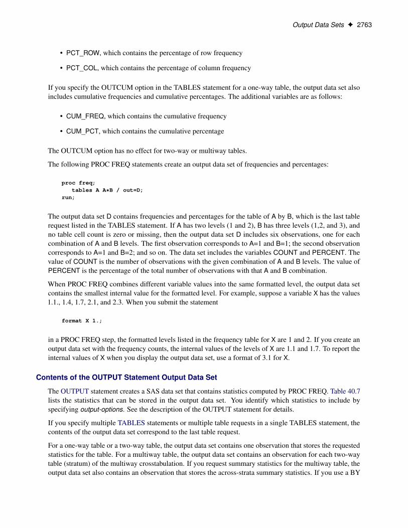
Output Data Sets F 2763
• PCT_ROW, which contains the percentage of row frequency
• PCT_COL, which contains the percentage of column frequency
If you specify the OUTCUM option in the TABLES statement for a one-way table, the output data set alsoincludes cumulative frequencies and cumulative percentages. The additional variables are as follows:
• CUM_FREQ, which contains the cumulative frequency
• CUM_PCT, which contains the cumulative percentage
The OUTCUM option has no effect for two-way or multiway tables.
The following PROC FREQ statements create an output data set of frequencies and percentages:
proc freq;tables A A*B / out=D;
run;
The output data set D contains frequencies and percentages for the table of A by B, which is the last tablerequest listed in the TABLES statement. If A has two levels (1 and 2), B has three levels (1,2, and 3), andno table cell count is zero or missing, then the output data set D includes six observations, one for eachcombination of A and B levels. The first observation corresponds to A=1 and B=1; the second observationcorresponds to A=1 and B=2; and so on. The data set includes the variables COUNT and PERCENT. Thevalue of COUNT is the number of observations with the given combination of A and B levels. The value ofPERCENT is the percentage of the total number of observations with that A and B combination.
When PROC FREQ combines different variable values into the same formatted level, the output data setcontains the smallest internal value for the formatted level. For example, suppose a variable X has the values1.1., 1.4, 1.7, 2.1, and 2.3. When you submit the statement
format X 1.;
in a PROC FREQ step, the formatted levels listed in the frequency table for X are 1 and 2. If you create anoutput data set with the frequency counts, the internal values of the levels of X are 1.1 and 1.7. To report theinternal values of X when you display the output data set, use a format of 3.1 for X.
Contents of the OUTPUT Statement Output Data Set
The OUTPUT statement creates a SAS data set that contains statistics computed by PROC FREQ. Table 40.7lists the statistics that can be stored in the output data set. You identify which statistics to include byspecifying output-options. See the description of the OUTPUT statement for details.
If you specify multiple TABLES statements or multiple table requests in a single TABLES statement, thecontents of the output data set correspond to the last table request.
For a one-way table or a two-way table, the output data set contains one observation that stores the requestedstatistics for the table. For a multiway table, the output data set contains an observation for each two-waytable (stratum) of the multiway crosstabulation. If you request summary statistics for the multiway table, theoutput data set also contains an observation that stores the across-strata summary statistics. If you use a BY
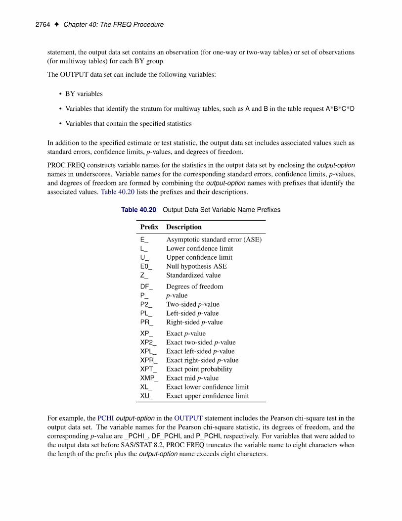
2764 F Chapter 40: The FREQ Procedure
statement, the output data set contains an observation (for one-way or two-way tables) or set of observations(for multiway tables) for each BY group.
The OUTPUT data set can include the following variables:
• BY variables
• Variables that identify the stratum for multiway tables, such as A and B in the table request A*B*C*D
• Variables that contain the specified statistics
In addition to the specified estimate or test statistic, the output data set includes associated values such asstandard errors, confidence limits, p-values, and degrees of freedom.
PROC FREQ constructs variable names for the statistics in the output data set by enclosing the output-optionnames in underscores. Variable names for the corresponding standard errors, confidence limits, p-values,and degrees of freedom are formed by combining the output-option names with prefixes that identify theassociated values. Table 40.20 lists the prefixes and their descriptions.
Table 40.20 Output Data Set Variable Name Prefixes
Prefix Description
E_ Asymptotic standard error (ASE)L_ Lower confidence limitU_ Upper confidence limitE0_ Null hypothesis ASEZ_ Standardized value
DF_ Degrees of freedomP_ p-valueP2_ Two-sided p-valuePL_ Left-sided p-valuePR_ Right-sided p-value
XP_ Exact p-valueXP2_ Exact two-sided p-valueXPL_ Exact left-sided p-valueXPR_ Exact right-sided p-valueXPT_ Exact point probabilityXMP_ Exact mid p-valueXL_ Exact lower confidence limitXU_ Exact upper confidence limit
For example, the PCHI output-option in the OUTPUT statement includes the Pearson chi-square test in theoutput data set. The variable names for the Pearson chi-square statistic, its degrees of freedom, and thecorresponding p-value are _PCHI_, DF_PCHI, and P_PCHI, respectively. For variables that were added tothe output data set before SAS/STAT 8.2, PROC FREQ truncates the variable name to eight characters whenthe length of the prefix plus the output-option name exceeds eight characters.

Displayed Output F 2765
Displayed Output
Number of Variable Levels Table
If you specify the NLEVELS option in the PROC FREQ statement, PROC FREQ displays the “Numberof Variable Levels” table. This table provides the number of levels for all variables named in the TABLESstatements. PROC FREQ determines the variable levels from the formatted variable values. See “Groupingwith Formats” on page 2698 for details. The “Number of Variable Levels” table contains the followinginformation:
• Variable name
• Levels, which is the total number of levels of the variable
• Number of Nonmissing Levels, if there are missing levels for any of the variables
• Number of Missing Levels, if there are missing levels for any of the variables
One-Way Frequency Tables
PROC FREQ displays one-way frequency tables for all one-way table requests in the TABLES statements,unless you specify the NOPRINT option in the PROC FREQ statement or the NOPRINT option in theTABLES statement. For a one-way table showing the frequency distribution of a single variable, PROCFREQ displays the name of the variable and its values. For each variable value or level, PROC FREQ displaysthe following information:
• Frequency count, which is the number of observations in the level
• Test Frequency count, if you specify the CHISQ and TESTF= options to request a chi-square goodness-of-fit test for specified frequencies
• Percent, which is the percentage of the total number of observations. (The NOPERCENT optionsuppresses this information.)
• Test Percent, if you specify the CHISQ and TESTP= options to request a chi-square goodness-of-fittest for specified percents. (The NOPERCENT option suppresses this information.)
• Cumulative Frequency count, which is the sum of the frequency counts for that level and all otherlevels listed above it in the table. The last cumulative frequency is the total number of nonmissingobservations. (The NOCUM option suppresses this information.)
• Cumulative Percent, which is the percentage of the total number of observations in that level and in allother levels listed above it in the table. (The NOCUM or the NOPERCENT option suppresses thisinformation.)
The one-way table also displays the Frequency Missing, which is the number of observations with missingvalues.
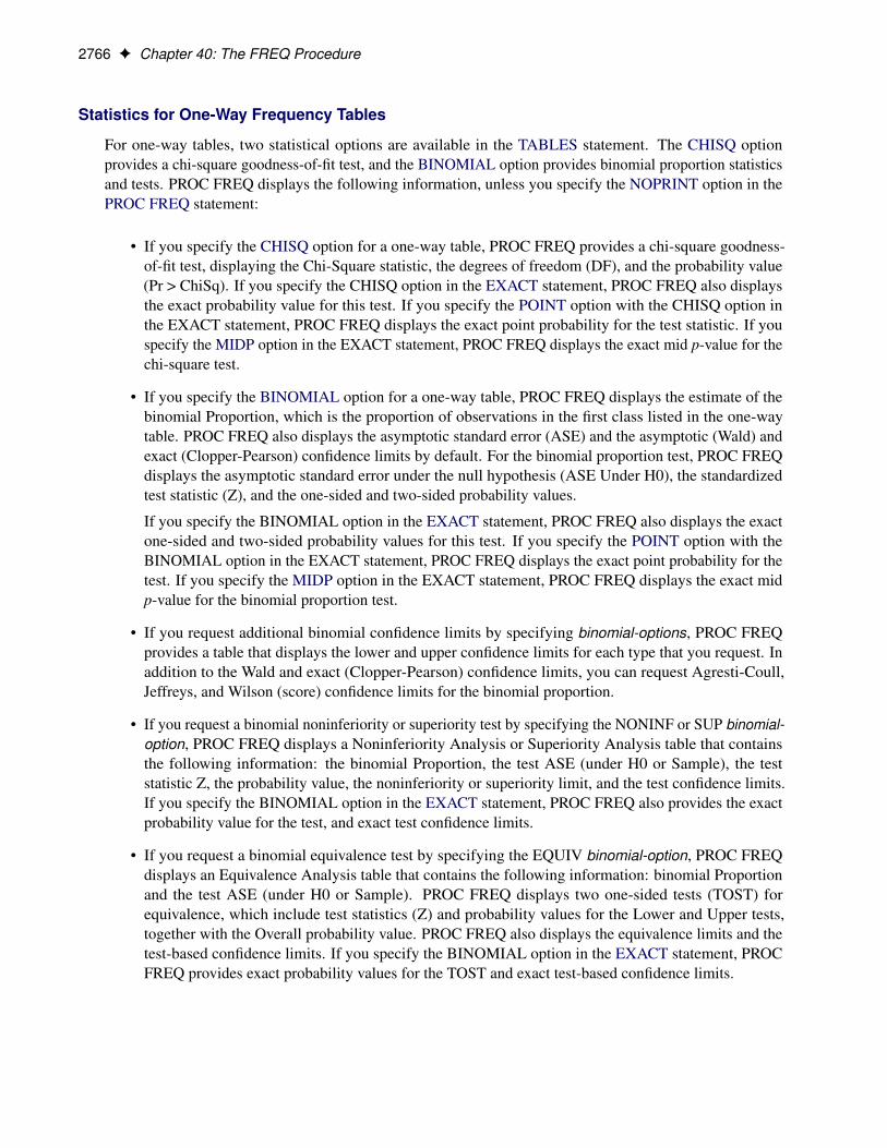
2766 F Chapter 40: The FREQ Procedure
Statistics for One-Way Frequency Tables
For one-way tables, two statistical options are available in the TABLES statement. The CHISQ optionprovides a chi-square goodness-of-fit test, and the BINOMIAL option provides binomial proportion statisticsand tests. PROC FREQ displays the following information, unless you specify the NOPRINT option in thePROC FREQ statement:
• If you specify the CHISQ option for a one-way table, PROC FREQ provides a chi-square goodness-of-fit test, displaying the Chi-Square statistic, the degrees of freedom (DF), and the probability value(Pr > ChiSq). If you specify the CHISQ option in the EXACT statement, PROC FREQ also displaysthe exact probability value for this test. If you specify the POINT option with the CHISQ option inthe EXACT statement, PROC FREQ displays the exact point probability for the test statistic. If youspecify the MIDP option in the EXACT statement, PROC FREQ displays the exact mid p-value for thechi-square test.
• If you specify the BINOMIAL option for a one-way table, PROC FREQ displays the estimate of thebinomial Proportion, which is the proportion of observations in the first class listed in the one-waytable. PROC FREQ also displays the asymptotic standard error (ASE) and the asymptotic (Wald) andexact (Clopper-Pearson) confidence limits by default. For the binomial proportion test, PROC FREQdisplays the asymptotic standard error under the null hypothesis (ASE Under H0), the standardizedtest statistic (Z), and the one-sided and two-sided probability values.
If you specify the BINOMIAL option in the EXACT statement, PROC FREQ also displays the exactone-sided and two-sided probability values for this test. If you specify the POINT option with theBINOMIAL option in the EXACT statement, PROC FREQ displays the exact point probability for thetest. If you specify the MIDP option in the EXACT statement, PROC FREQ displays the exact midp-value for the binomial proportion test.
• If you request additional binomial confidence limits by specifying binomial-options, PROC FREQprovides a table that displays the lower and upper confidence limits for each type that you request. Inaddition to the Wald and exact (Clopper-Pearson) confidence limits, you can request Agresti-Coull,Jeffreys, and Wilson (score) confidence limits for the binomial proportion.
• If you request a binomial noninferiority or superiority test by specifying the NONINF or SUP binomial-option, PROC FREQ displays a Noninferiority Analysis or Superiority Analysis table that containsthe following information: the binomial Proportion, the test ASE (under H0 or Sample), the teststatistic Z, the probability value, the noninferiority or superiority limit, and the test confidence limits.If you specify the BINOMIAL option in the EXACT statement, PROC FREQ also provides the exactprobability value for the test, and exact test confidence limits.
• If you request a binomial equivalence test by specifying the EQUIV binomial-option, PROC FREQdisplays an Equivalence Analysis table that contains the following information: binomial Proportionand the test ASE (under H0 or Sample). PROC FREQ displays two one-sided tests (TOST) forequivalence, which include test statistics (Z) and probability values for the Lower and Upper tests,together with the Overall probability value. PROC FREQ also displays the equivalence limits and thetest-based confidence limits. If you specify the BINOMIAL option in the EXACT statement, PROCFREQ provides exact probability values for the TOST and exact test-based confidence limits.

Displayed Output F 2767
Two-Way and Multiway Tables
PROC FREQ displays all multiway table requests in the TABLES statements, unless you specify theNOPRINT option in the PROC FREQ statement or the NOPRINT option in the TABLES statement.
For two-way to multiway crosstabulation tables, the values of the last variable in the table request form thetable columns. The values of the next-to-last variable form the rows. Each level (or combination of levels) ofthe other variables forms one stratum.
There are three ways to display multiway tables in PROC FREQ. By default, PROC FREQ displays multiwaytables as separate two-way crosstabulation tables for each stratum of the multiway table. Also by default,PROC FREQ displays these two-way crosstabulation tables in table cell format. Alternatively, if you specifythe CROSSLIST option, PROC FREQ displays the two-way crosstabulation tables in ODS column format. Ifyou specify the LIST option, PROC FREQ displays multiway tables in list format, which presents the entiremultiway crosstabulation in a single table.
Crosstabulation TablesBy default, PROC FREQ displays two-way crosstabulation tables in table cell format. The row variablevalues are listed down the side of the table, the column variable values are listed across the top of the table,and each row and column variable level combination forms a table cell.
Each cell of a crosstabulation table can contain the following information:
• Frequency, which is the number of observations in the table cell. (The NOFREQ option suppressesthis information.)
• Expected frequency under the hypothesis of independence, if you specify the EXPECTED option
• Deviation of the cell frequency from the expected value, if you specify the DEVIATION option
• Cell Chi-Square, which is the cell’s contribution to the total chi-square statistic, if you specify theCELLCHI2 option
• Tot Pct, which is the cell’s percentage of the total multiway table frequency, for n-way tables when n >2, if you specify the TOTPCT option
• Percent, which is the cell’s percentage of the total (two-way table) frequency. (The NOPERCENToption suppresses this information.)
• Row Pct, or the row percentage, which is the cell’s percentage of the total frequency for its row. (TheNOROW option suppresses this information.)
• Col Pct, or column percentage, which is the cell’s percentage of the total frequency for its column.(The NOCOL option suppresses this information.)
• Cumulative Col%, or cumulative column percentage, if you specify the CUMCOL option
The table also displays the Frequency Missing, which is the number of observations with missing values.

2768 F Chapter 40: The FREQ Procedure
CROSSLIST TablesIf you specify the CROSSLIST option, PROC FREQ displays two-way crosstabulation tables in ODS columnformat. The CROSSLIST column format is different from the default crosstabulation table cell format, butthe CROSSLIST table provides the same information (frequencies, percentages, and other statistics) as thedefault crosstabulation table.
In the CROSSLIST table format, the rows of the display correspond to the crosstabulation table cells, and thecolumns of the display correspond to descriptive statistics such as frequencies and percentages. Each tablecell is identified by the values of its TABLES row and column variable levels, with all column variable levelslisted within each row variable level. The CROSSLIST table also provides row totals, column totals, andoverall table totals.
For a crosstabulation table in CROSSLIST format, PROC FREQ displays the following information:
• the row variable name and values
• the column variable name and values
• Frequency, which is the number of observations in the table cell. (The NOFREQ option suppressesthis information.)
• Expected cell frequency under the hypothesis of independence, if you specify the EXPECTED option
• Deviation of the cell frequency from the expected value, if you specify the DEVIATION option
• Standardized Residual, if you specify the CROSSLIST(STDRES) option
• Pearson Residual, if you specify the CROSSLIST(PEARSONRES) option
• Cell Chi-Square, which is the cell’s contribution to the total chi-square statistic, if you specify theCELLCHI2 option
• Total Percent, which is the cell’s percentage of the total multiway table frequency, for n-way tableswhen n > 2, if you specify the TOTPCT option
• Percent, which is the cell’s percentage of the total (two-way table) frequency. (The NOPERCENToption suppresses this information.)
• Row Percent, which is the cell’s percentage of the total frequency for its row. (The NOROW optionsuppresses this information.)
• Column Percent, the cell’s percentage of the total frequency for its column. (The NOCOL optionsuppresses this information.)
The table also displays the Frequency Missing, which is the number of observations with missing values.
LIST TablesIf you specify the LIST option in the TABLES statement, PROC FREQ displays multiway tables in a listformat rather than as crosstabulation tables. The LIST option displays the entire multiway table in one table,instead of displaying a separate two-way table for each stratum. The LIST option is not available whenyou also request statistical options. Unlike the default crosstabulation output, the LIST output does not

Displayed Output F 2769
display row percentages, column percentages, and optional information such as expected frequencies and cellchi-squares.
For a multiway table in list format, PROC FREQ displays the following information:
• the variable names and values
• Frequency, which is the number of observations in the level (with the indicated variable values)
• Percent, which is the level’s percentage of the total number of observations. (The NOPERCENT optionsuppresses this information.)
• Cumulative Frequency, which is the accumulated frequency of the level and all other levels listedabove it in the table. The last cumulative frequency in the table is the total number of nonmissingobservations. (The NOCUM option suppresses this information.)
• Cumulative Percent, which is the accumulated percentage of the level and all other levels listed aboveit in the table. (The NOCUM or the NOPERCENT option suppresses this information.)
The table also displays the Frequency Missing, which is the number of observations with missing values.
Statistics for Two-Way and Multiway Tables
PROC FREQ computes statistical tests and measures for crosstabulation tables, depending on which state-ments and options you specify. You can suppress the display of these results by specifying the NOPRINToption in the PROC FREQ statement. With any of the following information, PROC FREQ also displays theSample Size and the Frequency Missing.
• If you specify the SCOROUT option in the TABLES statement, PROC FREQ displays the Row Scoresand Column Scores that it uses for statistical computations. The Row Scores table displays the rowvariable values and the Score corresponding to each value. The Column Scores table displays thecolumn variable values and the corresponding Scores. PROC FREQ also identifies the score type usedto compute the row and column scores. You can specify the score type with the SCORES= option inthe TABLES statement.
• If you specify the CHISQ option, PROC FREQ displays the following statistics for each two-way table:Pearson Chi-Square, Likelihood Ratio Chi-Square, Continuity-Adjusted Chi-Square (for 2 � 2 tables),Mantel-Haenszel Chi-Square, the Phi Coefficient, the Contingency Coefficient, and Cramér’s V. Foreach test statistic, PROC FREQ also displays the degrees of freedom (DF) and the probability value(Prob).
• If you specify the CHISQ option for 2 � 2 tables, PROC FREQ also displays Fisher’s exact test. Thetest output includes the cell (1,1) frequency (F), the exact left-sided and right-sided probability values,the table probability (P), and the exact two-sided probability value. If you specify the POINT option inthe EXACT statement, PROC FREQ displays the exact point probability for Fisher’s exact test. If youspecify the MIDP option in the EXACT statement, PROC FREQ displays the Mid p-Value for the test.
• If you specify the FISHER option in the TABLES statement (or, equivalently, the FISHER option inthe EXACT statement), PROC FREQ displays Fisher’s exact test for tables larger than 2 � 2. The testoutput includes the table probability (P) and the probability value. If you specify the POINT option inthe EXACT statement, PROC FREQ displays the exact point probability for Fisher’s exact test. If youspecify the MIDP option in the EXACT statement, PROC FREQ displays the Mid p-Value for the test.
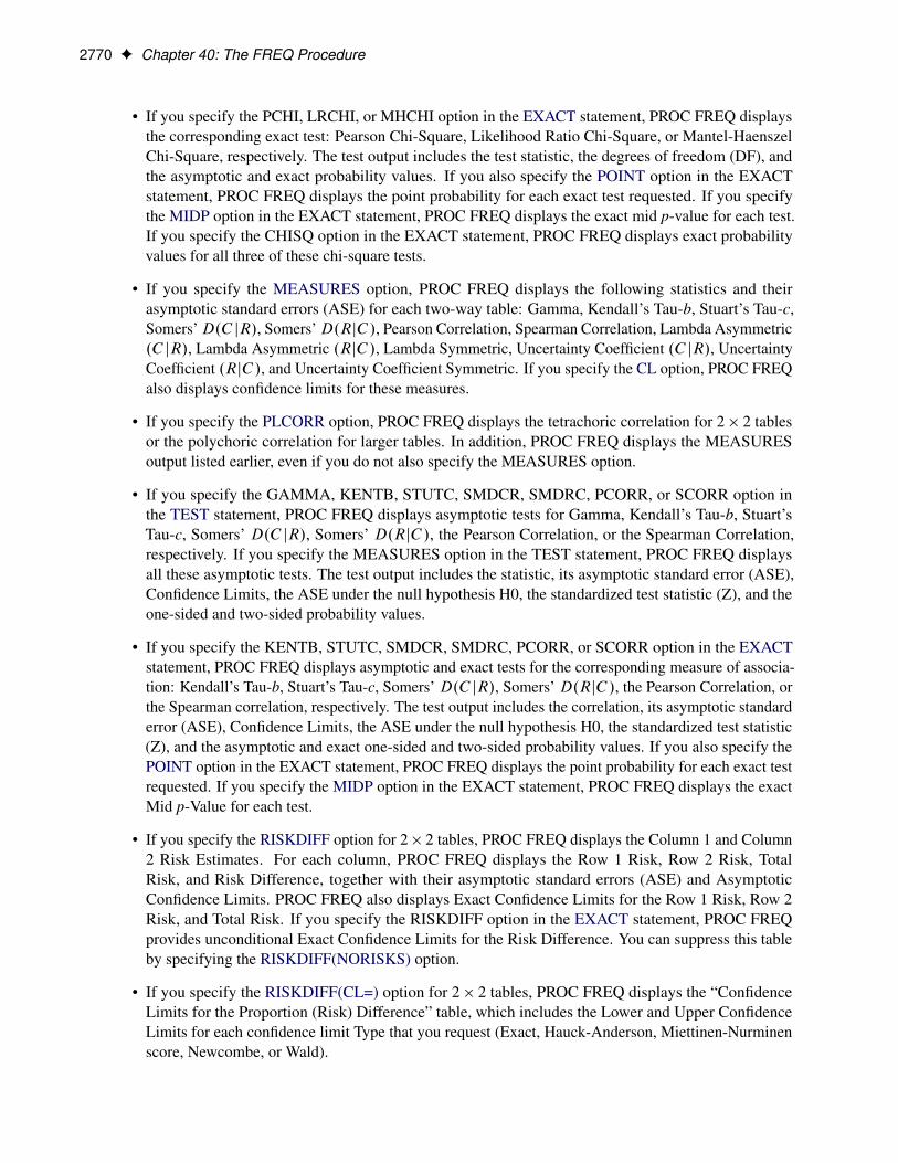
2770 F Chapter 40: The FREQ Procedure
• If you specify the PCHI, LRCHI, or MHCHI option in the EXACT statement, PROC FREQ displaysthe corresponding exact test: Pearson Chi-Square, Likelihood Ratio Chi-Square, or Mantel-HaenszelChi-Square, respectively. The test output includes the test statistic, the degrees of freedom (DF), andthe asymptotic and exact probability values. If you also specify the POINT option in the EXACTstatement, PROC FREQ displays the point probability for each exact test requested. If you specifythe MIDP option in the EXACT statement, PROC FREQ displays the exact mid p-value for each test.If you specify the CHISQ option in the EXACT statement, PROC FREQ displays exact probabilityvalues for all three of these chi-square tests.
• If you specify the MEASURES option, PROC FREQ displays the following statistics and theirasymptotic standard errors (ASE) for each two-way table: Gamma, Kendall’s Tau-b, Stuart’s Tau-c,Somers’D.C jR/, Somers’D.RjC/, Pearson Correlation, Spearman Correlation, Lambda Asymmetric.C jR/, Lambda Asymmetric .RjC/, Lambda Symmetric, Uncertainty Coefficient .C jR/, UncertaintyCoefficient .RjC/, and Uncertainty Coefficient Symmetric. If you specify the CL option, PROC FREQalso displays confidence limits for these measures.
• If you specify the PLCORR option, PROC FREQ displays the tetrachoric correlation for 2 � 2 tablesor the polychoric correlation for larger tables. In addition, PROC FREQ displays the MEASURESoutput listed earlier, even if you do not also specify the MEASURES option.
• If you specify the GAMMA, KENTB, STUTC, SMDCR, SMDRC, PCORR, or SCORR option inthe TEST statement, PROC FREQ displays asymptotic tests for Gamma, Kendall’s Tau-b, Stuart’sTau-c, Somers’ D.C jR/, Somers’ D.RjC/, the Pearson Correlation, or the Spearman Correlation,respectively. If you specify the MEASURES option in the TEST statement, PROC FREQ displaysall these asymptotic tests. The test output includes the statistic, its asymptotic standard error (ASE),Confidence Limits, the ASE under the null hypothesis H0, the standardized test statistic (Z), and theone-sided and two-sided probability values.
• If you specify the KENTB, STUTC, SMDCR, SMDRC, PCORR, or SCORR option in the EXACTstatement, PROC FREQ displays asymptotic and exact tests for the corresponding measure of associa-tion: Kendall’s Tau-b, Stuart’s Tau-c, Somers’ D.C jR/, Somers’ D.RjC/, the Pearson Correlation, orthe Spearman correlation, respectively. The test output includes the correlation, its asymptotic standarderror (ASE), Confidence Limits, the ASE under the null hypothesis H0, the standardized test statistic(Z), and the asymptotic and exact one-sided and two-sided probability values. If you also specify thePOINT option in the EXACT statement, PROC FREQ displays the point probability for each exact testrequested. If you specify the MIDP option in the EXACT statement, PROC FREQ displays the exactMid p-Value for each test.
• If you specify the RISKDIFF option for 2� 2 tables, PROC FREQ displays the Column 1 and Column2 Risk Estimates. For each column, PROC FREQ displays the Row 1 Risk, Row 2 Risk, TotalRisk, and Risk Difference, together with their asymptotic standard errors (ASE) and AsymptoticConfidence Limits. PROC FREQ also displays Exact Confidence Limits for the Row 1 Risk, Row 2Risk, and Total Risk. If you specify the RISKDIFF option in the EXACT statement, PROC FREQprovides unconditional Exact Confidence Limits for the Risk Difference. You can suppress this tableby specifying the RISKDIFF(NORISKS) option.
• If you specify the RISKDIFF(CL=) option for 2 � 2 tables, PROC FREQ displays the “ConfidenceLimits for the Proportion (Risk) Difference” table, which includes the Lower and Upper ConfidenceLimits for each confidence limit Type that you request (Exact, Hauck-Anderson, Miettinen-Nurminenscore, Newcombe, or Wald).
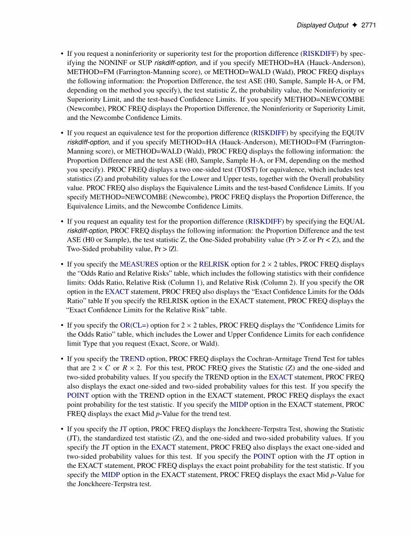
Displayed Output F 2771
• If you request a noninferiority or superiority test for the proportion difference (RISKDIFF) by spec-ifying the NONINF or SUP riskdiff-option, and if you specify METHOD=HA (Hauck-Anderson),METHOD=FM (Farrington-Manning score), or METHOD=WALD (Wald), PROC FREQ displaysthe following information: the Proportion Difference, the test ASE (H0, Sample, Sample H-A, or FM,depending on the method you specify), the test statistic Z, the probability value, the Noninferiority orSuperiority Limit, and the test-based Confidence Limits. If you specify METHOD=NEWCOMBE(Newcombe), PROC FREQ displays the Proportion Difference, the Noninferiority or Superiority Limit,and the Newcombe Confidence Limits.
• If you request an equivalence test for the proportion difference (RISKDIFF) by specifying the EQUIVriskdiff-option, and if you specify METHOD=HA (Hauck-Anderson), METHOD=FM (Farrington-Manning score), or METHOD=WALD (Wald), PROC FREQ displays the following information: theProportion Difference and the test ASE (H0, Sample, Sample H-A, or FM, depending on the methodyou specify). PROC FREQ displays a two one-sided test (TOST) for equivalence, which includes teststatistics (Z) and probability values for the Lower and Upper tests, together with the Overall probabilityvalue. PROC FREQ also displays the Equivalence Limits and the test-based Confidence Limits. If youspecify METHOD=NEWCOMBE (Newcombe), PROC FREQ displays the Proportion Difference, theEquivalence Limits, and the Newcombe Confidence Limits.
• If you request an equality test for the proportion difference (RISKDIFF) by specifying the EQUALriskdiff-option, PROC FREQ displays the following information: the Proportion Difference and the testASE (H0 or Sample), the test statistic Z, the One-Sided probability value (Pr > Z or Pr < Z), and theTwo-Sided probability value, Pr > |Z|.
• If you specify the MEASURES option or the RELRISK option for 2 � 2 tables, PROC FREQ displaysthe “Odds Ratio and Relative Risks” table, which includes the following statistics with their confidencelimits: Odds Ratio, Relative Risk (Column 1), and Relative Risk (Column 2). If you specify the ORoption in the EXACT statement, PROC FREQ also displays the “Exact Confidence Limits for the OddsRatio” table If you specify the RELRISK option in the EXACT statement, PROC FREQ displays the“Exact Confidence Limits for the Relative Risk” table.
• If you specify the OR(CL=) option for 2 � 2 tables, PROC FREQ displays the “Confidence Limits forthe Odds Ratio” table, which includes the Lower and Upper Confidence Limits for each confidencelimit Type that you request (Exact, Score, or Wald).
• If you specify the TREND option, PROC FREQ displays the Cochran-Armitage Trend Test for tablesthat are 2 � C or R � 2. For this test, PROC FREQ gives the Statistic (Z) and the one-sided andtwo-sided probability values. If you specify the TREND option in the EXACT statement, PROC FREQalso displays the exact one-sided and two-sided probability values for this test. If you specify thePOINT option with the TREND option in the EXACT statement, PROC FREQ displays the exactpoint probability for the test statistic. If you specify the MIDP option in the EXACT statement, PROCFREQ displays the exact Mid p-Value for the trend test.
• If you specify the JT option, PROC FREQ displays the Jonckheere-Terpstra Test, showing the Statistic(JT), the standardized test statistic (Z), and the one-sided and two-sided probability values. If youspecify the JT option in the EXACT statement, PROC FREQ also displays the exact one-sided andtwo-sided probability values for this test. If you specify the POINT option with the JT option inthe EXACT statement, PROC FREQ displays the exact point probability for the test statistic. If youspecify the MIDP option in the EXACT statement, PROC FREQ displays the exact Mid p-Value forthe Jonckheere-Terpstra test.

2772 F Chapter 40: The FREQ Procedure
• If you specify the AGREE(PRINTKWTS) option, PROC FREQ displays the Kappa Coefficient Weightsfor square tables of dimension greater than 2.
• If you specify the AGREE option, for two-way tables PROC FREQ displays McNemar’s Test and theSimple Kappa Coefficient for 2 � 2 tables. For square tables larger than 2 � 2, PROC FREQ displaysBowker’s Test of Symmetry, the Simple Kappa Coefficient, and the Weighted Kappa Coefficient. ForMcNemar’s Test and Bowker’s Test of Symmetry, PROC FREQ displays the Statistic (S), the degreesof freedom (DF), and For the simple and weighted kappa coefficients, PROC FREQ displays the kappavalues, asymptotic standard errors (ASE), and Confidence Limits. the probability value (Pr > S).
If you specify the MCNEM option in the EXACT statement, PROC FREQ also displays the exactprobability value for McNemar’s test. If you specify the POINT option with the MCNEM option inthe EXACT statement, PROC FREQ displays the exact point probability for the test statistic. If youspecify the MIDP option in the EXACT statement, PROC FREQ displays the Exact Mid p-Value forMcNemar’s test.
• If you specify the KAPPA or WTKAP option in the TEST statement, PROC FREQ displays asymptotictests for the simple kappa coefficient or the weighted kappa coefficient, respectively. If you specifythe AGREE option in the TEST statement, PROC FREQ displays both these asymptotic tests. Thetest output includes the kappa coefficient, its asymptotic standard error (ASE), Confidence Limits, theASE under the null hypothesis H0, the standardized test statistic (Z), and the one-sided and two-sidedprobability values.
• If you specify the KAPPA or WTKAP option in the EXACT statement, PROC FREQ displays asymp-totic and exact tests for the simple kappa coefficient or the weighted kappa coefficient, respectively.The test output includes the kappa coefficient, its asymptotic standard error (ASE), Confidence Limits,the ASE under the null hypothesis H0, the standardized test statistic (Z), and the asymptotic and exactone-sided and two-sided probability values. If you specify the POINT option in the EXACT statement,PROC FREQ displays the point probability for each exact test requested. If you specify the MIDPoption in the EXACT statement, PROC FREQ displays the exact Mid p-Value for each exact test.
• If you specify the MC option in the EXACT statement, PROC FREQ displays Monte Carlo estimatesfor all exact p-values requested by statistic-options in the EXACT statement. The Monte Carlo outputincludes the p-value Estimate, its Confidence Limits, the Number of Samples used to compute theMonte Carlo estimate, and the Initial Seed for random number generation.
• If you specify the AGREE option for a multiway square table, PROC FREQ displays Overall Simpleand Weighted Kappa Coefficients, with their asymptotic standard errors (ASE) and Confidence Limits.PROC FREQ also displays Tests for Equal Kappa Coefficients, giving the Chi-Squares, degrees offreedom (DF), and probability values (Pr > ChiSq) for the Simple Kappa and Weighted Kappa. Formultiple strata of 2 � 2 tables, PROC FREQ displays Cochran’s Q, giving the Statistic (Q), the degreesof freedom (DF), and the probability value (Pr > Q).
• If you specify the RISKDIFF(COMMON) option for a multiway 2 � 2 table, PROC FREQ displaysthe “Common Proportion (Risk) Difference” table, which includes the following information: Method(Mantel-Haenszel or Summary Score), Value of the common risk difference, Standard Error, andConfidence Limits.
• If you specify the CMH option, PROC FREQ displays Cochran-Mantel-Haenszel Statistics for thefollowing three alternative hypotheses: Nonzero Correlation, Row Mean Scores Differ (ANOVAStatistic), and General Association. For each of these statistics, PROC FREQ gives the degrees of

ODS Table Names F 2773
freedom (DF) and the probability value (Prob). If you specify the MANTELFLEISS option, PROCFREQ displays the Mantel-Fleiss Criterion for 2�2 tables. For 2�2 tables, PROC FREQ also displaysEstimates of the Common Relative Risk for Case-Control and Cohort studies, together with theirconfidence limits. These include both Mantel-Haenszel and Logit stratum-adjusted estimates of thecommon Odds Ratio, Column 1 Relative Risk, and Column 2 Relative Risk. Also for 2 � 2 tables,PROC FREQ displays the Breslow-Day Test for Homogeneity of the Odds Ratios. For this test, PROCFREQ gives the Chi-Square, the degrees of freedom (DF), and the probability value (Pr > ChiSq).
• If you specify the CMH option in the TABLES statement and also specify the COMOR option in theEXACT statement for a multiway 2�2 table, PROC FREQ displays exact confidence limits for the Com-mon Odds Ratio. PROC FREQ also displays the Exact Test of H0: Common Odds Ratio = 1. The testoutput includes the Cell (1,1) Sum (S), Mean of S Under H0, One-sided Pr <= S, and Point Pr = S.PROC FREQ also provides exact two-sided probability values for the test, computed accordingto the following three methods: 2 * One-sided, Sum of probabilities <= Point probability, andPr >= |S - Mean|. If you specify the MIDP option in the EXACT statement, PROC FREQ provides theexact Mid p-Value for the common odds ratio test.
• If you specify the CMH option in the TABLES statement and also specify the EQOR option in theEXACT statement for a multiway 2� 2 table, PROC FREQ computes Zelen’s exact test for equal oddsratios. PROC FREQ displays Zelen’s test along with the asymptotic Breslow-Day test produced by theCMH option. PROC FREQ displays the test statistic, Zelen’s Exact Test (P), and the probability value,Exact Pr <= P.
• If you specify the GAILSIMON option in the TABLES statement for a multiway 2 � 2 tables, PROCFREQ displays the Gail-Simon test for qualitative interactions. The display include the followingstatistics and their p-values: Q+ (Positive Risk Differences), Q- (Negative Risk Differences), and Q(Two-Sided).
ODS Table NamesPROC FREQ assigns a name to each table that it creates. You can use these names to refer to tables whenyou use the Output Delivery System (ODS) to select tables and create output data sets. For more informationabout ODS, see Chapter 20, “Using the Output Delivery System.”
Table 40.21 lists the ODS table names together with their descriptions and the options required to producethe tables. Note that the ALL option in the TABLES statement invokes the CHISQ, MEASURES, and CMHoptions.
Table 40.21 ODS Tables Produced by PROC FREQ
ODS Table Name Description Statement Option
BarnardsTest Barnard’s exact test EXACT BARNARDBinomialCLs Binomial confidence limits TABLES BINOMIAL(AC | J | W)BinomialEquiv Binomial equivalence analysis TABLES BINOMIAL(EQUIV)BinomialEquivLimits Binomial equivalence limits TABLES BINOMIAL(EQUIV)BinomialEquivTest Binomial equivalence test TABLES BINOMIAL(EQUIV)BinomialNoninf Binomial noninferiority test TABLES BINOMIAL(NONINF)Binomial Binomial proportion TABLES BINOMIALBinomialTest Binomial proportion test TABLES BINOMIAL
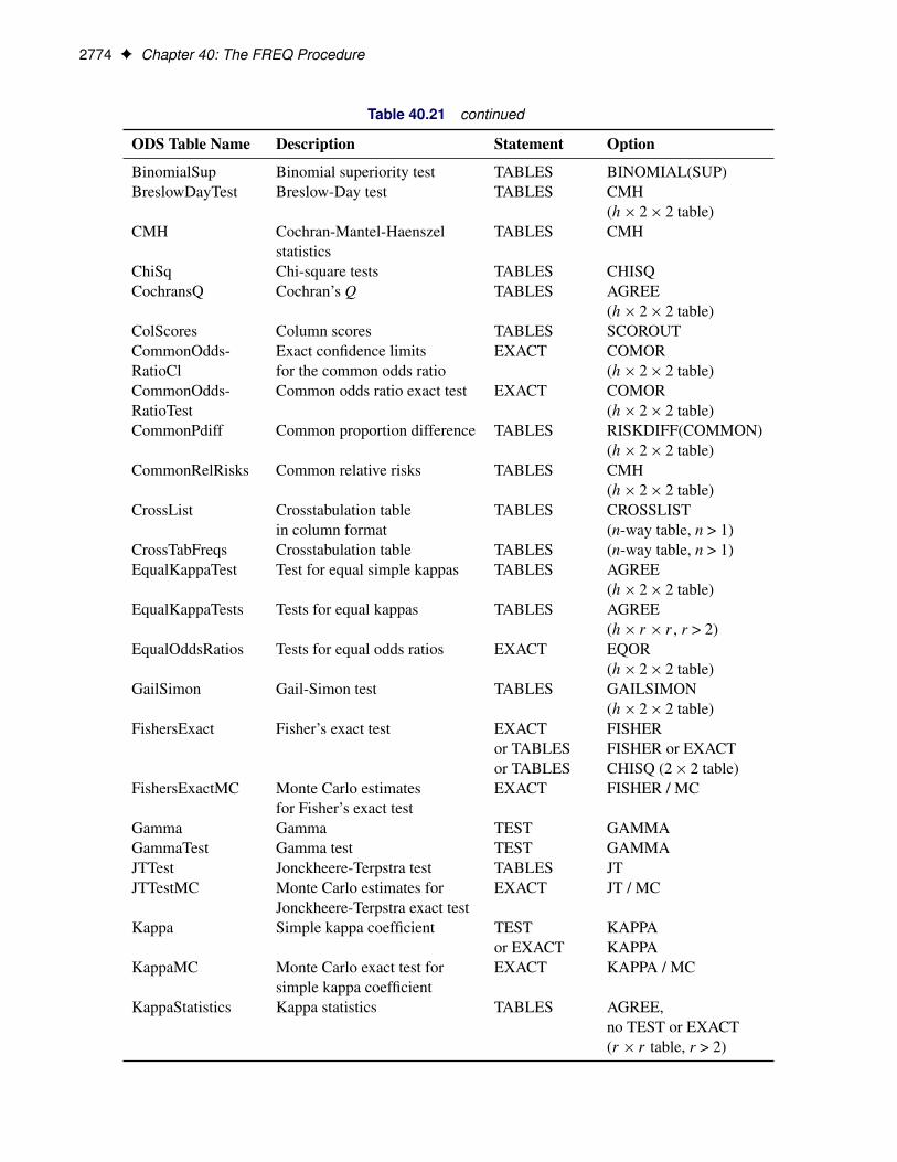
2774 F Chapter 40: The FREQ Procedure
Table 40.21 continued
ODS Table Name Description Statement Option
BinomialSup Binomial superiority test TABLES BINOMIAL(SUP)BreslowDayTest Breslow-Day test TABLES CMH
(h � 2 � 2 table)CMH Cochran-Mantel-Haenszel TABLES CMH
statisticsChiSq Chi-square tests TABLES CHISQCochransQ Cochran’s Q TABLES AGREE
(h � 2 � 2 table)ColScores Column scores TABLES SCOROUTCommonOdds- Exact confidence limits EXACT COMORRatioCl for the common odds ratio (h � 2 � 2 table)CommonOdds- Common odds ratio exact test EXACT COMORRatioTest (h � 2 � 2 table)CommonPdiff Common proportion difference TABLES RISKDIFF(COMMON)
(h � 2 � 2 table)CommonRelRisks Common relative risks TABLES CMH
(h � 2 � 2 table)CrossList Crosstabulation table TABLES CROSSLIST
in column format (n-way table, n > 1)CrossTabFreqs Crosstabulation table TABLES (n-way table, n > 1)EqualKappaTest Test for equal simple kappas TABLES AGREE
(h � 2 � 2 table)EqualKappaTests Tests for equal kappas TABLES AGREE
(h � r � r , r > 2)EqualOddsRatios Tests for equal odds ratios EXACT EQOR
(h � 2 � 2 table)GailSimon Gail-Simon test TABLES GAILSIMON
(h � 2 � 2 table)FishersExact Fisher’s exact test EXACT FISHER
or TABLES FISHER or EXACTor TABLES CHISQ (2 � 2 table)
FishersExactMC Monte Carlo estimates EXACT FISHER / MCfor Fisher’s exact test
Gamma Gamma TEST GAMMAGammaTest Gamma test TEST GAMMAJTTest Jonckheere-Terpstra test TABLES JTJTTestMC Monte Carlo estimates for EXACT JT / MC
Jonckheere-Terpstra exact testKappa Simple kappa coefficient TEST KAPPA
or EXACT KAPPAKappaMC Monte Carlo exact test for EXACT KAPPA / MC
simple kappa coefficientKappaStatistics Kappa statistics TABLES AGREE,
no TEST or EXACT(r � r table, r > 2)

ODS Table Names F 2775
Table 40.21 continued
ODS Table Name Description Statement Option
KappaTest Simple kappa test TEST KAPPAor EXACT KAPPA
KappaWeights Kappa weights TABLES AGREE(PRINTKWTS)List List format multiway table TABLES LISTLRChiSq Likelihood ratio chi-square EXACT LRCHI
exact testLRChiSqMC Monte Carlo exact test for EXACT LRCHI / MC
likelihood ratio chi-squareMantelFleiss Mantel-Fleiss criterion TABLES CMH(MF)
(h � 2 � 2 table)McNemarsTest McNemar’s test TABLES AGREE
(2 � 2 table)Measures Measures of association TABLES MEASURESMHChiSq Mantel-Haenszel chi-square EXACT MHCHI
exact testMHChiSqMC Monte Carlo exact test for EXACT MHCHI / MC
Mantel-Haenszel chi-squareNLevels Number of variable levels PROC NLEVELSOddsRatioCLs Odds ratio confidence limits TABLES OR(CL=) (2 � 2 table)OddsRatioExactCL Exact confidence limits EXACT OR (2 � 2 table)
for the odds ratioOneWayChiSq One-way chi-square test TABLES CHISQ
(one-way table)OneWayChiSqMC Monte Carlo exact test for EXACT CHISQ / MC
one-way chi-square (one-way table)OneWayFreqs One-way frequencies PROC (no TABLES stmt)
or TABLES (one-way table)OneWayLRChiSq One-way likelihood ratio TABLES CHISQ(LRCHI)
chi-square test (one-way table)OverallKappa Overall simple kappa TABLES AGREE
(h � 2 � 2 table)OverallKappas Overall kappa coefficients TABLES AGREE
(h � r � r , r > 2)PdiffCLs Proportion difference TABLES RISKDIFF(CL=)
confidence limits (2 � 2 table)PdiffEquiv Equivalence analysis TABLES RISKDIFF(EQUIV)
for the proportion difference (2 � 2 table)PdiffEquivLimits Equivalence limits TABLES RISKDIFF(EQUIV)
for the proportion difference (2 � 2 table)PdiffEquivTest Equivalence test TABLES RISKDIFF(EQUIV)
for the proportion difference (2 � 2 table)PdiffNoninf Noninferiority test TABLES RISKDIFF(NONINF)
for the proportion difference (2 � 2 table)PdiffSup Superiority test TABLES RISKDIFF(SUP)
for the proportion difference (2 � 2 table)
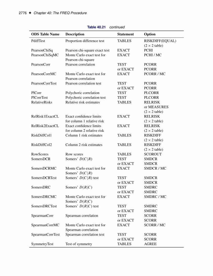
2776 F Chapter 40: The FREQ Procedure
Table 40.21 continued
ODS Table Name Description Statement Option
PdiffTest Proportion difference test TABLES RISKDIFF(EQUAL)(2 � 2 table)
PearsonChiSq Pearson chi-square exact test EXACT PCHIPearsonChiSqMC Monte Carlo exact test for EXACT PCHI / MC
Pearson chi-squarePearsonCorr Pearson correlation TEST PCORR
or EXACT PCORRPearsonCorrMC Monte Carlo exact test for EXACT PCORR / MC
Pearson correlationPearsonCorrTest Pearson correlation test TEST PCORR
or EXACT PCORRPlCorr Polychoric correlation TEST PLCORRPlCorrTest Polychoric correlation test TEST PLCORRRelativeRisks Relative risk estimates TABLES RELRISK
or MEASURES(2 � 2 table)
RelRisk1ExactCL Exact confidence limits EXACT RELRISKfor column 1 relative risk (2 � 2 table)
RelRisk2ExactCL Exact confidence limits EXACT RELRISKfor column 2 relative risk (2 � 2 table)
RiskDiffCol1 Column 1 risk estimates TABLES RISKDIFF(2 � 2 table)
RiskDiffCol2 Column 2 risk estimates TABLES RISKDIFF(2 � 2 table)
RowScores Row scores TABLES SCOROUTSomersDCR Somers’ D.C jR/ TEST SMDCR
or EXACT SMDCRSomersDCRMC Monte Carlo exact test for EXACT SMDCR / MC
Somers’ D.C jR/SomersDCRTest Somers’ D.C jR/ test TEST SMDCR
or EXACT SMDCRSomersDRC Somers’ D.RjC/ TEST SMDRC
or EXACT SMDRCSomersDRCMC Monte Carlo exact test for EXACT SMDRC / MC
Somers’ D.RjC/SomersDRCTest Somers’ D.RjC/ test TEST SMDRC
or EXACT SMDRCSpearmanCorr Spearman correlation TEST SCORR
or EXACT SCORRSpearmanCorrMC Monte Carlo exact test for EXACT SCORR / MC
Spearman correlationSpearmanCorrTest Spearman correlation test TEST SCORR
or EXACT SCORRSymmetryTest Test of symmetry TABLES AGREE

ODS Graphics F 2777
Table 40.21 continued
ODS Table Name Description Statement Option
TauB Kendall’s tau-b TEST KENTBor EXACT KENTB
TauBMC Monte Carlo exact test for EXACT KENTB / MCKendall’s tau-b
TauBTest Kendall’s tau-b test TEST KENTBor EXACT KENTB
TauC Stuart’s tau-c TEST STUTCor EXACT STUTC
TauCMC Monte Carlo exact test for EXACT STUTC / MCStuart’s tau-c
TauCTest Stuart’s tau-c test TEST STUTCor EXACT STUTC
TrendTest Cochran-Armitage trend test TABLES TRENDTrendTestMC Monte Carlo exact test EXACT TREND / MC
for trendWtKappa Weighted kappa coefficient TEST WTKAP
or EXACT WTKAPWtKappaMC Monte Carlo exact test for EXACT WTKAP / MC
weighted kappa coefficientWtKappaTest Weighted kappa test TEST WTKAP
or EXACT WTKAP
ODS GraphicsStatistical procedures use ODS Graphics to create graphs as part of their output. ODS Graphics is describedin detail in Chapter 21, “Statistical Graphics Using ODS.”
Before you create graphs, ODS Graphics must be enabled (for example, by specifying the ODS GRAPH-ICS ON statement). For more information about enabling and disabling ODS Graphics, see the section“Enabling and Disabling ODS Graphics” on page 606 in Chapter 21, “Statistical Graphics Using ODS.”
The overall appearance of graphs is controlled by ODS styles. Styles and other aspects of using ODSGraphics are discussed in the section “A Primer on ODS Statistical Graphics” on page 605 in Chapter 21,“Statistical Graphics Using ODS.”
When ODS Graphics is enabled, you can request specific plots with the PLOTS= option in the TABLESstatement. To produce a frequency plot or cumulative frequency plot, you must specify the FREQPLOT orCUMFREQPLOT plot-request , respectively, in the PLOTS= option. To produce a mosaic plot, you mustspecify the MOSAICPLOT plot-request in the PLOTS= option. You can also produce frequency, cumulativefrequency, and mosaic plots by specifying the PLOTS=ALL option. By default, PROC FREQ produces allother plots that are associated with the analyses that you request in the TABLES statement. You can suppressthe default plots and request specific plots by using the PLOTS(ONLY)= option. See the description of thePLOTS= option for details.

2778 F Chapter 40: The FREQ Procedure
PROC FREQ assigns a name to each graph that it creates with ODS Graphics. You can use these names torefer to the graphs. Table 40.22 lists the names of the graphs that PROC FREQ generates together with theirdescriptions, their PLOTS= options (plot-requests), and the TABLES statement options that are required toproduce the graphs.
Table 40.22 Graphs Produced by PROC FREQ
ODS Graph Name Description PLOTS= Option TABLES Statement Option
AgreePlot Agreement plot AGREEPLOT AGREE (r � r table)CumFreqPlot Cumulative frequency plot CUMFREQPLOT One-way table requestDeviationPlot Deviation plot DEVIATIONPLOT CHISQ (one-way table)FreqPlot Frequency plot FREQPLOT Any table requestKappaPlot Kappa plot KAPPAPLOT AGREE (h � r � r table)MosaicPlot Mosaic plot MOSAICPLOT Two-way or multiway table requestORPlot Odds ratio plot ODDSRATIOPLOT MEASURES or RELRISK
(h � 2 � 2 table)RelRiskPlot Relative risk plot RELRISKPLOT MEASURES or RELRISK
(h � 2 � 2 table)RiskDiffPlot Risk difference plot RISKDIFFPLOT RISKDIFF (h � 2 � 2 table)WtKappaPlot Weighted kappa plot WTKAPPAPLOT AGREE
(h � r � r table, r > 2)
Examples: FREQ Procedure
Example 40.1: Output Data Set of FrequenciesThe eye and hair color of children from two different regions of Europe are recorded in the data set Color.Instead of recording one observation per child, the data are recorded as cell counts, where the variable Countcontains the number of children exhibiting each of the 15 eye and hair color combinations. The data set doesnot include missing combinations.
The following DATA step statements create the SAS data set Color:
data Color;input Region Eyes $ Hair $ Count @@;label Eyes ='Eye Color'
Hair ='Hair Color'Region='Geographic Region';
datalines;1 blue fair 23 1 blue red 7 1 blue medium 241 blue dark 11 1 green fair 19 1 green red 71 green medium 18 1 green dark 14 1 brown fair 341 brown red 5 1 brown medium 41 1 brown dark 401 brown black 3 2 blue fair 46 2 blue red 212 blue medium 44 2 blue dark 40 2 blue black 62 green fair 50 2 green red 31 2 green medium 372 green dark 23 2 brown fair 56 2 brown red 422 brown medium 53 2 brown dark 54 2 brown black 13;
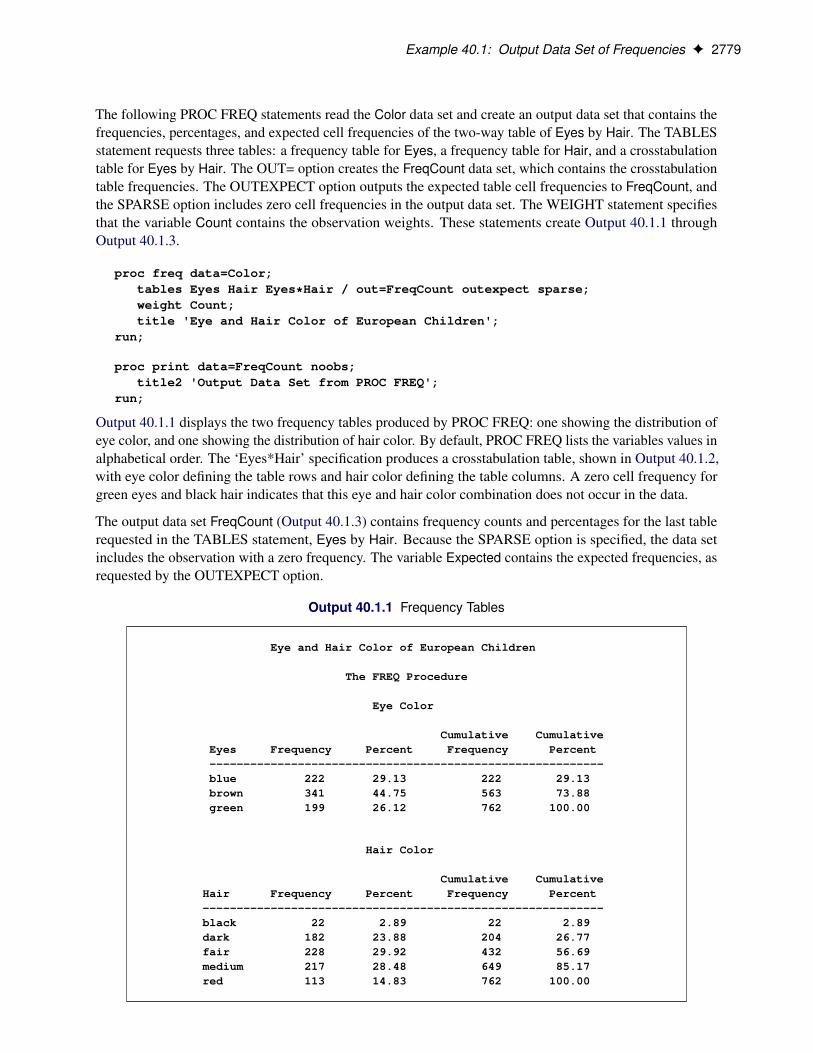
Example 40.1: Output Data Set of Frequencies F 2779
The following PROC FREQ statements read the Color data set and create an output data set that contains thefrequencies, percentages, and expected cell frequencies of the two-way table of Eyes by Hair. The TABLESstatement requests three tables: a frequency table for Eyes, a frequency table for Hair, and a crosstabulationtable for Eyes by Hair. The OUT= option creates the FreqCount data set, which contains the crosstabulationtable frequencies. The OUTEXPECT option outputs the expected table cell frequencies to FreqCount, andthe SPARSE option includes zero cell frequencies in the output data set. The WEIGHT statement specifiesthat the variable Count contains the observation weights. These statements create Output 40.1.1 throughOutput 40.1.3.
proc freq data=Color;tables Eyes Hair Eyes*Hair / out=FreqCount outexpect sparse;weight Count;title 'Eye and Hair Color of European Children';
run;
proc print data=FreqCount noobs;title2 'Output Data Set from PROC FREQ';
run;
Output 40.1.1 displays the two frequency tables produced by PROC FREQ: one showing the distribution ofeye color, and one showing the distribution of hair color. By default, PROC FREQ lists the variables values inalphabetical order. The ‘Eyes*Hair’ specification produces a crosstabulation table, shown in Output 40.1.2,with eye color defining the table rows and hair color defining the table columns. A zero cell frequency forgreen eyes and black hair indicates that this eye and hair color combination does not occur in the data.
The output data set FreqCount (Output 40.1.3) contains frequency counts and percentages for the last tablerequested in the TABLES statement, Eyes by Hair. Because the SPARSE option is specified, the data setincludes the observation with a zero frequency. The variable Expected contains the expected frequencies, asrequested by the OUTEXPECT option.
Output 40.1.1 Frequency Tables
Eye and Hair Color of European Children
The FREQ Procedure
Eye Color
Cumulative CumulativeEyes Frequency Percent Frequency Percent----------------------------------------------------------blue 222 29.13 222 29.13brown 341 44.75 563 73.88green 199 26.12 762 100.00
Hair Color
Cumulative CumulativeHair Frequency Percent Frequency Percent-----------------------------------------------------------black 22 2.89 22 2.89dark 182 23.88 204 26.77fair 228 29.92 432 56.69medium 217 28.48 649 85.17red 113 14.83 762 100.00
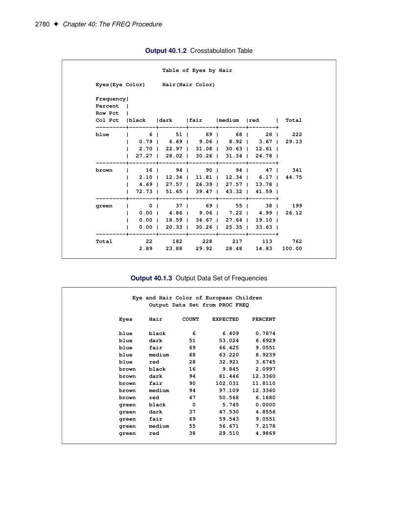
2780 F Chapter 40: The FREQ Procedure
Output 40.1.2 Crosstabulation Table
Table of Eyes by Hair
Eyes(Eye Color) Hair(Hair Color)
Frequency|Percent |Row Pct |Col Pct |black |dark |fair |medium |red | Total---------+--------+--------+--------+--------+--------+blue | 6 | 51 | 69 | 68 | 28 | 222
| 0.79 | 6.69 | 9.06 | 8.92 | 3.67 | 29.13| 2.70 | 22.97 | 31.08 | 30.63 | 12.61 || 27.27 | 28.02 | 30.26 | 31.34 | 24.78 |
---------+--------+--------+--------+--------+--------+brown | 16 | 94 | 90 | 94 | 47 | 341
| 2.10 | 12.34 | 11.81 | 12.34 | 6.17 | 44.75| 4.69 | 27.57 | 26.39 | 27.57 | 13.78 || 72.73 | 51.65 | 39.47 | 43.32 | 41.59 |
---------+--------+--------+--------+--------+--------+green | 0 | 37 | 69 | 55 | 38 | 199
| 0.00 | 4.86 | 9.06 | 7.22 | 4.99 | 26.12| 0.00 | 18.59 | 34.67 | 27.64 | 19.10 || 0.00 | 20.33 | 30.26 | 25.35 | 33.63 |
---------+--------+--------+--------+--------+--------+Total 22 182 228 217 113 762
2.89 23.88 29.92 28.48 14.83 100.00
Output 40.1.3 Output Data Set of Frequencies
Eye and Hair Color of European ChildrenOutput Data Set from PROC FREQ
Eyes Hair COUNT EXPECTED PERCENT
blue black 6 6.409 0.7874blue dark 51 53.024 6.6929blue fair 69 66.425 9.0551blue medium 68 63.220 8.9239blue red 28 32.921 3.6745brown black 16 9.845 2.0997brown dark 94 81.446 12.3360brown fair 90 102.031 11.8110brown medium 94 97.109 12.3360brown red 47 50.568 6.1680green black 0 5.745 0.0000green dark 37 47.530 4.8556green fair 69 59.543 9.0551green medium 55 56.671 7.2178green red 38 29.510 4.9869

Example 40.2: Frequency Dot Plots F 2781
Example 40.2: Frequency Dot PlotsThis example produces frequency dot plots for the children’s eye and hair color data from Example 40.1.
PROC FREQ produces plots by using ODS Graphics to create graphs as part of the procedure output.Frequency plots are available for any frequency or crosstabulation table request. You can display frequencyplots as bar charts or dot plots. You can use plot-options to specify the orientation (vertical or horizontal),scale, and layout of the plots.
The following PROC FREQ statements request frequency tables and dot plots. The first TABLES statementrequests a one-way frequency table of Hair and a crosstabulation table of Eyes by Hair. The PLOTS= optionrequests frequency plots for the tables, and the TYPE=DOTPLOT plot-option specifies dot plots. By default,frequency plots are produced as bar charts. ODS Graphics must be enabled before producing plots.
The second TABLES statement requests a crosstabulation table of Region by Hair and a frequency dot plot forthis table. The SCALE=PERCENT plot-option plots percentages instead of frequency counts. SCALE=LOGand SCALE=SQRT plot-options are also available to plot log frequencies and square roots of frequencies,respectively.
The ORDER=FREQ option in the PROC FREQ statement orders the variable levels by frequency. This orderapplies to the frequency and crosstabulation table displays and also to the corresponding frequency plots.
ods graphics on;proc freq data=Color order=freq;
tables Hair Hair*Eyes / plots=freqplot(type=dotplot);tables Hair*Region / plots=freqplot(type=dotplot scale=percent);weight Count;title 'Eye and Hair Color of European Children';
run;ods graphics off;
Output 40.2.1, Output 40.2.2, and Output 40.2.3 display the dot plots produced by PROC FREQ. By default,the orientation of dot plots is horizontal, which places the variable levels on the Y axis. You can specifythe ORIENT=VERTICAL plot-option to request a vertical orientation. For two-way plots, you can usethe TWOWAY= plot-option to specify the plot layout. The default layout (shown in Output 40.2.2 andOutput 40.2.3) is GROUPVERTICAL. Two-way layouts STACKED and GROUPHORIZONTAL are alsoavailable.

2782 F Chapter 40: The FREQ Procedure
Output 40.2.1 One-Way Frequency Dot Plot
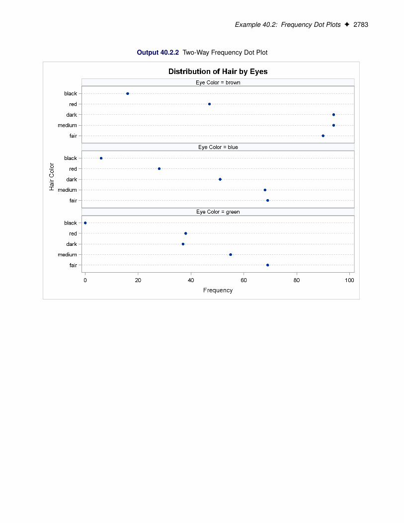
Example 40.2: Frequency Dot Plots F 2783
Output 40.2.2 Two-Way Frequency Dot Plot
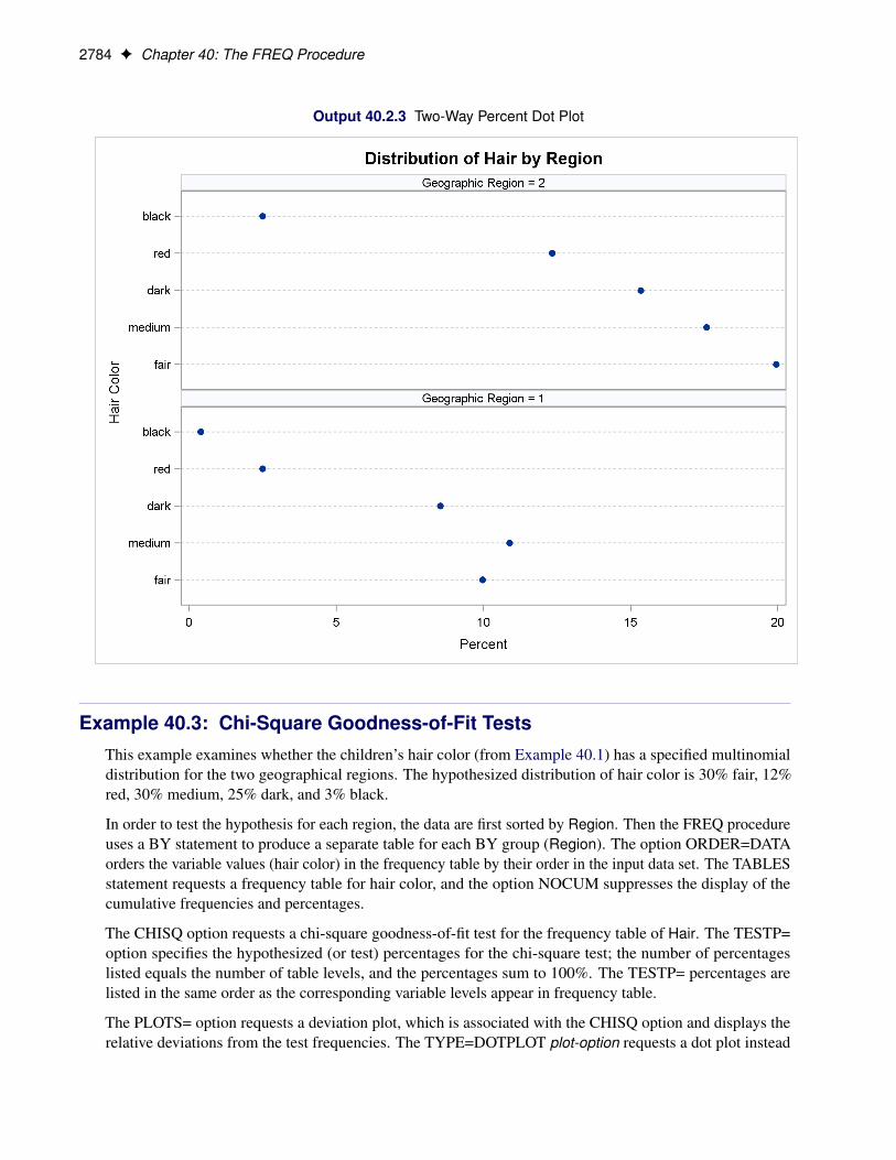
2784 F Chapter 40: The FREQ Procedure
Output 40.2.3 Two-Way Percent Dot Plot
Example 40.3: Chi-Square Goodness-of-Fit TestsThis example examines whether the children’s hair color (from Example 40.1) has a specified multinomialdistribution for the two geographical regions. The hypothesized distribution of hair color is 30% fair, 12%red, 30% medium, 25% dark, and 3% black.
In order to test the hypothesis for each region, the data are first sorted by Region. Then the FREQ procedureuses a BY statement to produce a separate table for each BY group (Region). The option ORDER=DATAorders the variable values (hair color) in the frequency table by their order in the input data set. The TABLESstatement requests a frequency table for hair color, and the option NOCUM suppresses the display of thecumulative frequencies and percentages.
The CHISQ option requests a chi-square goodness-of-fit test for the frequency table of Hair. The TESTP=option specifies the hypothesized (or test) percentages for the chi-square test; the number of percentageslisted equals the number of table levels, and the percentages sum to 100%. The TESTP= percentages arelisted in the same order as the corresponding variable levels appear in frequency table.
The PLOTS= option requests a deviation plot, which is associated with the CHISQ option and displays therelative deviations from the test frequencies. The TYPE=DOTPLOT plot-option requests a dot plot instead
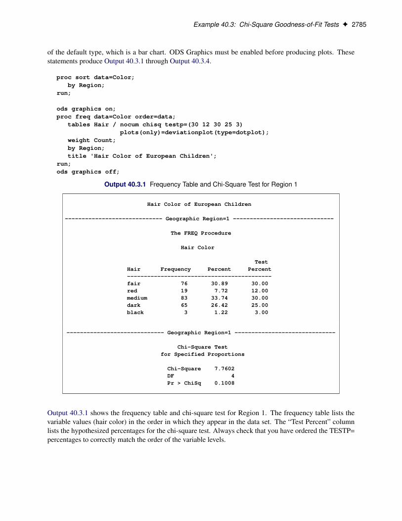
Example 40.3: Chi-Square Goodness-of-Fit Tests F 2785
of the default type, which is a bar chart. ODS Graphics must be enabled before producing plots. Thesestatements produce Output 40.3.1 through Output 40.3.4.
proc sort data=Color;by Region;
run;
ods graphics on;proc freq data=Color order=data;
tables Hair / nocum chisq testp=(30 12 30 25 3)plots(only)=deviationplot(type=dotplot);
weight Count;by Region;title 'Hair Color of European Children';
run;ods graphics off;
Output 40.3.1 Frequency Table and Chi-Square Test for Region 1
Hair Color of European Children
----------------------------- Geographic Region=1 ------------------------------
The FREQ Procedure
Hair Color
TestHair Frequency Percent Percent-------------------------------------------fair 76 30.89 30.00red 19 7.72 12.00medium 83 33.74 30.00dark 65 26.42 25.00black 3 1.22 3.00
----------------------------- Geographic Region=1 ------------------------------
Chi-Square Testfor Specified Proportions
Chi-Square 7.7602DF 4Pr > ChiSq 0.1008
Output 40.3.1 shows the frequency table and chi-square test for Region 1. The frequency table lists thevariable values (hair color) in the order in which they appear in the data set. The “Test Percent” columnlists the hypothesized percentages for the chi-square test. Always check that you have ordered the TESTP=percentages to correctly match the order of the variable levels.
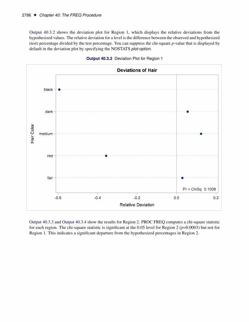
2786 F Chapter 40: The FREQ Procedure
Output 40.3.2 shows the deviation plot for Region 1, which displays the relative deviations from thehypothesized values. The relative deviation for a level is the difference between the observed and hypothesized(test) percentage divided by the test percentage. You can suppress the chi-square p-value that is displayed bydefault in the deviation plot by specifying the NOSTATS plot-option.
Output 40.3.2 Deviation Plot for Region 1
Output 40.3.3 and Output 40.3.4 show the results for Region 2. PROC FREQ computes a chi-square statisticfor each region. The chi-square statistic is significant at the 0.05 level for Region 2 (p=0.0003) but not forRegion 1. This indicates a significant departure from the hypothesized percentages in Region 2.

Example 40.3: Chi-Square Goodness-of-Fit Tests F 2787
Output 40.3.3 Frequency Table and Chi-Square Test for Region 2
Hair Color of European Children
----------------------------- Geographic Region=2 ------------------------------
The FREQ Procedure
Hair Color
TestHair Frequency Percent Percent-------------------------------------------fair 152 29.46 30.00red 94 18.22 12.00medium 134 25.97 30.00dark 117 22.67 25.00black 19 3.68 3.00
----------------------------- Geographic Region=2 ------------------------------
Chi-Square Testfor Specified Proportions
Chi-Square 21.3824DF 4Pr > ChiSq 0.0003
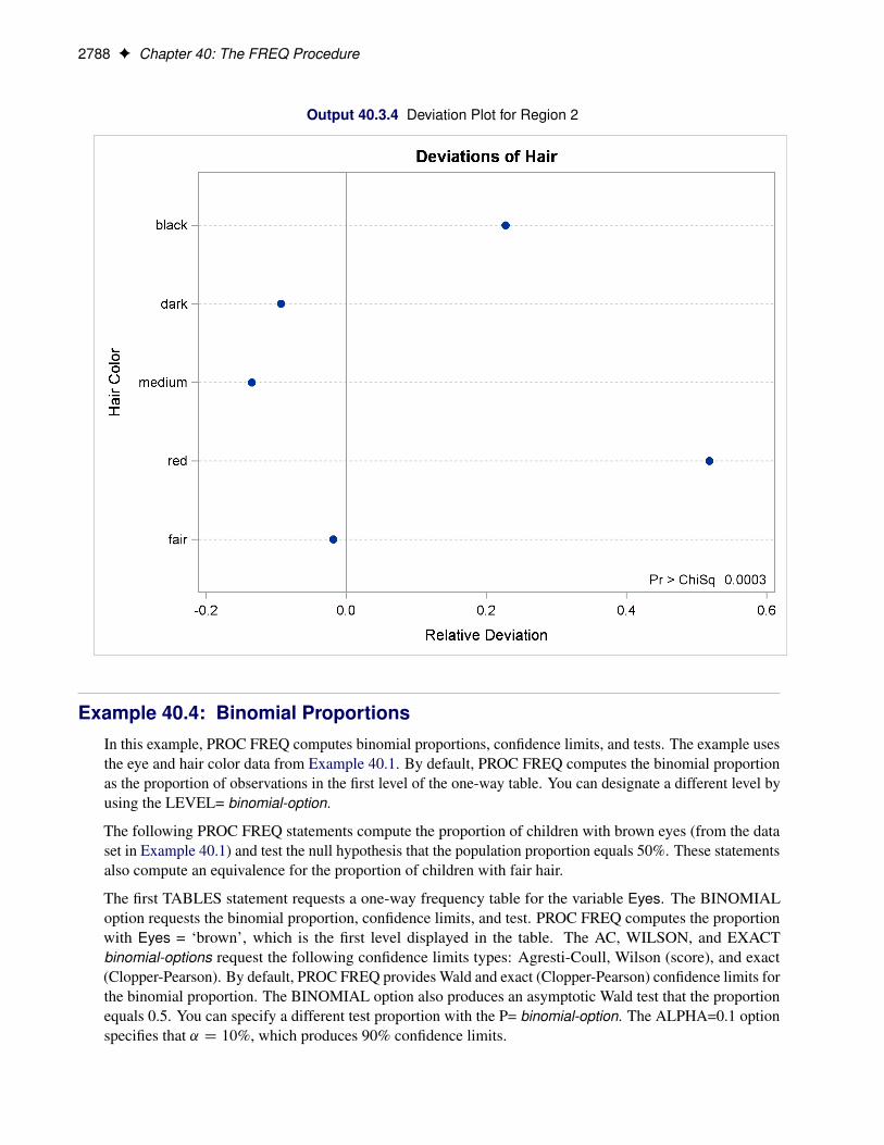
2788 F Chapter 40: The FREQ Procedure
Output 40.3.4 Deviation Plot for Region 2
Example 40.4: Binomial ProportionsIn this example, PROC FREQ computes binomial proportions, confidence limits, and tests. The example usesthe eye and hair color data from Example 40.1. By default, PROC FREQ computes the binomial proportionas the proportion of observations in the first level of the one-way table. You can designate a different level byusing the LEVEL= binomial-option.
The following PROC FREQ statements compute the proportion of children with brown eyes (from the dataset in Example 40.1) and test the null hypothesis that the population proportion equals 50%. These statementsalso compute an equivalence for the proportion of children with fair hair.
The first TABLES statement requests a one-way frequency table for the variable Eyes. The BINOMIALoption requests the binomial proportion, confidence limits, and test. PROC FREQ computes the proportionwith Eyes = ‘brown’, which is the first level displayed in the table. The AC, WILSON, and EXACTbinomial-options request the following confidence limits types: Agresti-Coull, Wilson (score), and exact(Clopper-Pearson). By default, PROC FREQ provides Wald and exact (Clopper-Pearson) confidence limits forthe binomial proportion. The BINOMIAL option also produces an asymptotic Wald test that the proportionequals 0.5. You can specify a different test proportion with the P= binomial-option. The ALPHA=0.1 optionspecifies that ˛ D 10%, which produces 90% confidence limits.

Example 40.4: Binomial Proportions F 2789
The second TABLES statement requests a one-way frequency table for the variable Hair. The BINOMIALoption requests the proportion for the first level, Hair = ‘fair’. The EQUIV binomial-option requests anequivalence test for the binomial proportion. The P=.28 option specifies 0.28 as the null hypothesis proportion,and the MARGIN=.1 option specifies 0.1 as the equivalence test margin.
proc freq data=Color order=freq;tables Eyes / binomial(ac wilson exact) alpha=.1;tables Hair / binomial(equiv p=.28 margin=.1);weight Count;title 'Hair and Eye Color of European Children';
run;
Output 40.4.1 displays the results for eye color, and Output 40.4.2 displays the results for hair color.
Output 40.4.1 Binomial Proportion for Eye Color
Hair and Eye Color of European Children
The FREQ Procedure
Eye Color
Cumulative CumulativeEyes Frequency Percent Frequency Percent----------------------------------------------------------brown 341 44.75 341 44.75blue 222 29.13 563 73.88green 199 26.12 762 100.00
Binomial ProportionEyes = brown
Proportion 0.4475ASE 0.0180
Type 90% Confidence Limits
Wilson 0.4181 0.4773Agresti-Coull 0.4181 0.4773Clopper-Pearson (Exact) 0.4174 0.4779
Test of H0: Proportion = 0.5
ASE under H0 0.0181Z -2.8981One-sided Pr < Z 0.0019Two-sided Pr > |Z| 0.0038
The frequency table in Output 40.4.1 displays the values of Eyes in order of descending frequency count.PROC FREQ computes the proportion of children in the first level displayed in the frequency table, Eyes =‘brown’. Output 40.4.1 displays the binomial proportion confidence limits and test. The confidence limits are
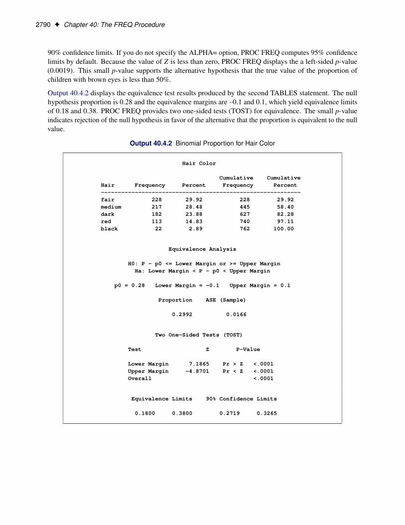
2790 F Chapter 40: The FREQ Procedure
90% confidence limits. If you do not specify the ALPHA= option, PROC FREQ computes 95% confidencelimits by default. Because the value of Z is less than zero, PROC FREQ displays the a left-sided p-value(0.0019). This small p-value supports the alternative hypothesis that the true value of the proportion ofchildren with brown eyes is less than 50%.
Output 40.4.2 displays the equivalence test results produced by the second TABLES statement. The nullhypothesis proportion is 0.28 and the equivalence margins are –0.1 and 0.1, which yield equivalence limitsof 0.18 and 0.38. PROC FREQ provides two one-sided tests (TOST) for equivalence. The small p-valueindicates rejection of the null hypothesis in favor of the alternative that the proportion is equivalent to the nullvalue.
Output 40.4.2 Binomial Proportion for Hair Color
Hair Color
Cumulative CumulativeHair Frequency Percent Frequency Percent-----------------------------------------------------------fair 228 29.92 228 29.92medium 217 28.48 445 58.40dark 182 23.88 627 82.28red 113 14.83 740 97.11black 22 2.89 762 100.00
Equivalence Analysis
H0: P - p0 <= Lower Margin or >= Upper MarginHa: Lower Margin < P - p0 < Upper Margin
p0 = 0.28 Lower Margin = -0.1 Upper Margin = 0.1
Proportion ASE (Sample)
0.2992 0.0166
Two One-Sided Tests (TOST)
Test Z P-Value
Lower Margin 7.1865 Pr > Z <.0001Upper Margin -4.8701 Pr < Z <.0001Overall <.0001
Equivalence Limits 90% Confidence Limits
0.1800 0.3800 0.2719 0.3265

Example 40.5: Analysis of a 2x2 Contingency Table F 2791
Example 40.5: Analysis of a 2x2 Contingency TableThis example computes chi-square tests and Fisher’s exact test to compare the probability of coronary heartdisease for two types of diet. It also estimates the relative risks and computes exact confidence limits for theodds ratio.
The data set FatComp contains hypothetical data for a case-control study of high fat diet and the risk ofcoronary heart disease. The data are recorded as cell counts, where the variable Count contains the frequenciesfor each exposure and response combination. The data set is sorted in descending order by the variablesExposure and Response, so that the first cell of the 2 � 2 table contains the frequency of positive exposureand positive response. The FORMAT procedure creates formats to identify the type of exposure and responsewith character values.
proc format;value ExpFmt 1='High Cholesterol Diet'
0='Low Cholesterol Diet';value RspFmt 1='Yes'
0='No';run;
data FatComp;input Exposure Response Count;label Response='Heart Disease';datalines;
0 0 60 1 21 0 41 1 11;
proc sort data=FatComp;by descending Exposure descending Response;
run;
In the following PROC FREQ statements, ORDER=DATA option orders the contingency table values by theirorder in the input data set. The TABLES statement requests a two-way table of Exposure by Response. TheCHISQ option produces several chi-square tests, while the RELRISK option produces relative risk measures.The EXACT statement requests the exact Pearson chi-square test and exact confidence limits for the oddsratio.
proc freq data=FatComp order=data;format Exposure ExpFmt. Response RspFmt.;tables Exposure*Response / chisq relrisk;exact pchi or;weight Count;title 'Case-Control Study of High Fat/Cholesterol Diet';
run;

2792 F Chapter 40: The FREQ Procedure
The contingency table in Output 40.5.1 displays the variable values so that the first table cell contains thefrequency for the first cell in the data set (the frequency of positive exposure and positive response).
Output 40.5.1 Contingency Table
Case-Control Study of High Fat/Cholesterol Diet
The FREQ Procedure
Table of Exposure by Response
Exposure Response(Heart Disease)
Frequency |Percent |Row Pct |Col Pct |Yes |No | Total-----------------+--------+--------+High Cholesterol | 11 | 4 | 15Diet | 47.83 | 17.39 | 65.22
| 73.33 | 26.67 || 84.62 | 40.00 |
-----------------+--------+--------+Low Cholesterol | 2 | 6 | 8Diet | 8.70 | 26.09 | 34.78
| 25.00 | 75.00 || 15.38 | 60.00 |
-----------------+--------+--------+Total 13 10 23
56.52 43.48 100.00
Output 40.5.2 displays the chi-square statistics. Because the expected counts in some of the table cells aresmall, PROC FREQ gives a warning that the asymptotic chi-square tests might not be appropriate. In thiscase, the exact tests are appropriate. The alternative hypothesis for this analysis states that coronary heartdisease is more likely to be associated with a high fat diet, so a one-sided test is desired. Fisher’s exactright-sided test analyzes whether the probability of heart disease in the high fat group exceeds the probabilityof heart disease in the low fat group; because this p-value is small, the alternative hypothesis is supported.
The odds ratio, displayed in Output 40.5.3, provides an estimate of the relative risk when an event is rare.This estimate indicates that the odds of heart disease is 8.25 times higher in the high fat diet group; however,the wide confidence limits indicate that this estimate has low precision.
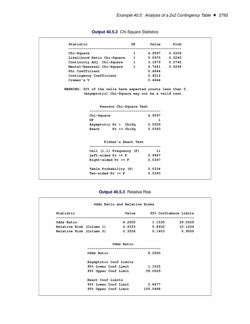
Example 40.5: Analysis of a 2x2 Contingency Table F 2793
Output 40.5.2 Chi-Square Statistics
Statistic DF Value Prob------------------------------------------------------Chi-Square 1 4.9597 0.0259Likelihood Ratio Chi-Square 1 5.0975 0.0240Continuity Adj. Chi-Square 1 3.1879 0.0742Mantel-Haenszel Chi-Square 1 4.7441 0.0294Phi Coefficient 0.4644Contingency Coefficient 0.4212Cramer's V 0.4644
WARNING: 50% of the cells have expected counts less than 5.(Asymptotic) Chi-Square may not be a valid test.
Pearson Chi-Square Test----------------------------------Chi-Square 4.9597DF 1Asymptotic Pr > ChiSq 0.0259Exact Pr >= ChiSq 0.0393
Fisher's Exact Test----------------------------------Cell (1,1) Frequency (F) 11Left-sided Pr <= F 0.9967Right-sided Pr >= F 0.0367
Table Probability (P) 0.0334Two-sided Pr <= P 0.0393
Output 40.5.3 Relative Risk
Odds Ratio and Relative Risks
Statistic Value 95% Confidence Limits------------------------------------------------------------------Odds Ratio 8.2500 1.1535 59.0029Relative Risk (Column 1) 2.9333 0.8502 10.1204Relative Risk (Column 2) 0.3556 0.1403 0.9009
Odds Ratio-----------------------------------Odds Ratio 8.2500
Asymptotic Conf Limits95% Lower Conf Limit 1.153595% Upper Conf Limit 59.0029
Exact Conf Limits95% Lower Conf Limit 0.867795% Upper Conf Limit 105.5488

2794 F Chapter 40: The FREQ Procedure
Example 40.6: Output Data Set of Chi-Square StatisticsThis example uses the Color data from Example 40.1 to output the Pearson chi-square and the likelihoodratio chi-square statistics to a SAS data set. The following PROC FREQ statements create a two-way table ofeye color versus hair color.
proc freq data=Color order=data;tables Eyes*Hair / expected cellchi2 norow nocol chisq;output out=ChiSqData n nmiss pchi lrchi;weight Count;title 'Chi-Square Tests for 3 by 5 Table of Eye and Hair Color';
run;
proc print data=ChiSqData noobs;title1 'Chi-Square Statistics for Eye and Hair Color';title2 'Output Data Set from the FREQ Procedure';
run;
The EXPECTED option displays expected cell frequencies in the crosstabulation table, and the CELLCHI2option displays the cell contribution to the overall chi-square. The NOROW and NOCOL options suppressthe display of row and column percents in the crosstabulation table. The CHISQ option produces chi-squaretests.
The OUTPUT statement creates the ChiSqData output data set and specifies the statistics to include. The Noption requests the number of nonmissing observations, the NMISS option stores the number of missingobservations, and the PCHI and LRCHI options request Pearson and likelihood ratio chi-square statistics,respectively, together with their degrees of freedom and p-values.
The preceding statements produce Output 40.6.1 and Output 40.6.2. The contingency table in Output 40.6.1displays eye and hair color in the order in which they appear in the Color data set. The Pearson chi-squarestatistic in Output 40.6.2 provides evidence of an association between eye and hair color (p=0.0073). Thecell chi-square values show that most of the association is due to more green-eyed children with fair or redhair and fewer with dark or black hair. The opposite occurs with the brown-eyed children.
Output 40.6.3 displays the output data set created by the OUTPUT statement. It includes one observationthat contains the sample size, the number of missing values, and the chi-square statistics and correspondingdegrees of freedom and p-values as in Output 40.6.2.

Example 40.6: Output Data Set of Chi-Square Statistics F 2795
Output 40.6.1 Contingency Table
Chi-Square Tests for 3 by 5 Table of Eye and Hair Color
The FREQ Procedure
Table of Eyes by Hair
Eyes(Eye Color) Hair(Hair Color)
Frequency |Expected |Cell Chi-Square|Percent |fair |red |medium |dark |black | Total---------------+--------+--------+--------+--------+--------+blue | 69 | 28 | 68 | 51 | 6 | 222
| 66.425 | 32.921 | 63.22 | 53.024 | 6.4094 || 0.0998 | 0.7357 | 0.3613 | 0.0772 | 0.0262 || 9.06 | 3.67 | 8.92 | 6.69 | 0.79 | 29.13
---------------+--------+--------+--------+--------+--------+green | 69 | 38 | 55 | 37 | 0 | 199
| 59.543 | 29.51 | 56.671 | 47.53 | 5.7454 || 1.5019 | 2.4422 | 0.0492 | 2.3329 | 5.7454 || 9.06 | 4.99 | 7.22 | 4.86 | 0.00 | 26.12
---------------+--------+--------+--------+--------+--------+brown | 90 | 47 | 94 | 94 | 16 | 341
| 102.03 | 50.568 | 97.109 | 81.446 | 9.8451 || 1.4187 | 0.2518 | 0.0995 | 1.935 | 3.8478 || 11.81 | 6.17 | 12.34 | 12.34 | 2.10 | 44.75
---------------+--------+--------+--------+--------+--------+Total 228 113 217 182 22 762
29.92 14.83 28.48 23.88 2.89 100.00
Output 40.6.2 Chi-Square Statistics
Statistic DF Value Prob------------------------------------------------------Chi-Square 8 20.9248 0.0073Likelihood Ratio Chi-Square 8 25.9733 0.0011Mantel-Haenszel Chi-Square 1 3.7838 0.0518Phi Coefficient 0.1657Contingency Coefficient 0.1635Cramer's V 0.1172
Output 40.6.3 Output Data Set
Chi-Square Statistics for Eye and Hair ColorOutput Data Set from the FREQ Procedure
N NMISS _PCHI_ DF_PCHI P_PCHI _LRCHI_ DF_LRCHI P_LRCHI
762 0 20.9248 8 .007349898 25.9733 8 .001061424

2796 F Chapter 40: The FREQ Procedure
Example 40.7: Cochran-Mantel-Haenszel StatisticsThe data set Migraine contains hypothetical data for a clinical trial of migraine treatment. Subjects of bothgenders receive either a new drug therapy or a placebo. Their response to treatment is coded as ‘Better’ or‘Same’. The data are recorded as cell counts, and the number of subjects for each treatment and responsecombination is recorded in the variable Count.
data Migraine;input Gender $ Treatment $ Response $ Count @@;datalines;
female Active Better 16 female Active Same 11female Placebo Better 5 female Placebo Same 20male Active Better 12 male Active Same 16male Placebo Better 7 male Placebo Same 19;
The following PROC FREQ statements create a multiway table stratified by Gender, where Treatment formsthe rows and Response forms the columns. The RELRISK option in the TABLES statement requests theodds ratio and relative risks for the two-way tables of Treatment by Response. The PLOTS= option requestsa relative risk plot, which shows the relative risk and its confidence limits for each level of Gender and overall.The CMH option requests Cochran-Mantel-Haenszel statistics for the multiway table. For this stratified 2� 2table, the CMH option also produces estimates of the common relative risk and the Breslow-Day test forhomogeneity of the odds ratios. The NOPRINT option suppresses the display of the crosstabulation tables.
ods graphics on;proc freq data=Migraine;
tables Gender*Treatment*Response /relrisk plots(only)=relriskplot(stats) cmh noprint;
weight Count;title 'Clinical Trial for Treatment of Migraine Headaches';
run;ods graphics off;
Output 40.7.1 through Output 40.7.4 show the results of the analysis. The relative risk plot (Output 40.7.1)displays the relative risks and confidence limits for the two levels of Gender and for the overall (common)relative risk. Output 40.7.2 displays the CMH statistics. For a stratified 2 � 2 table, the three CMH statisticstest the same hypothesis. The significant p-value (0.004) indicates that the association between treatment andresponse remains strong after adjusting for gender.
The CMH option also produces a table of overall relative risks, as shown in Output 40.7.3. Because this is aprospective study, the relative risk estimate assesses the effectiveness of the new drug; the “Cohort (Col1Risk)” values are the appropriate estimates for the first column (the risk of improvement). The probabilityof migraine improvement with the new drug is just over two times the probability of improvement with theplacebo.
The large p-value for the Breslow-Day test (0.2218) in Output 40.7.4 indicates no significant gender differencein the odds ratios.
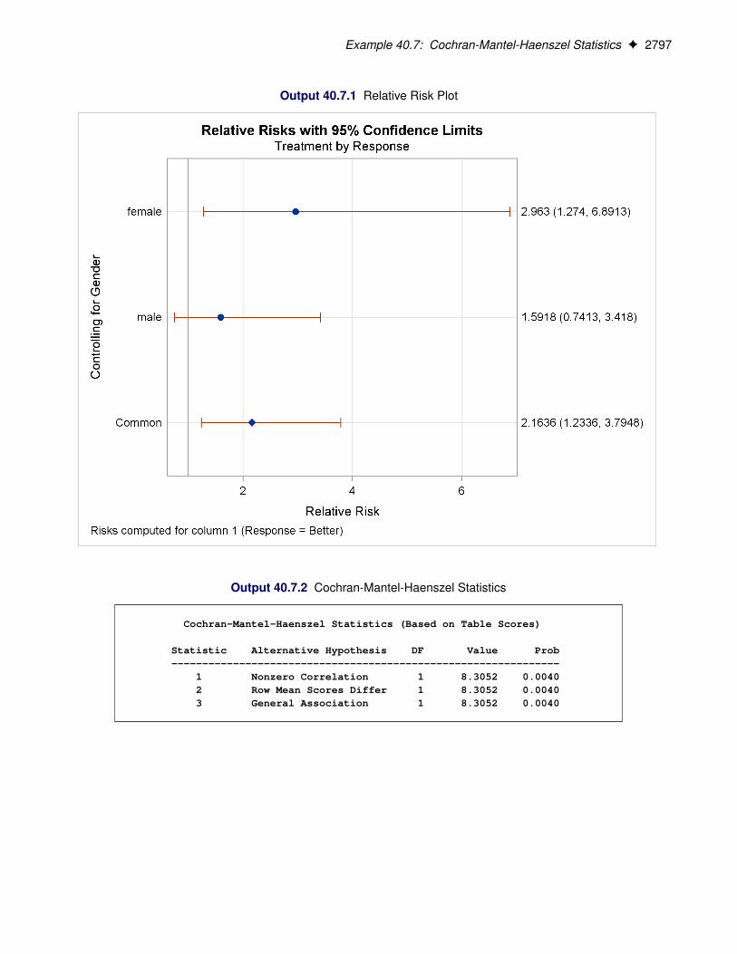
Example 40.7: Cochran-Mantel-Haenszel Statistics F 2797
Output 40.7.1 Relative Risk Plot
Output 40.7.2 Cochran-Mantel-Haenszel Statistics
Cochran-Mantel-Haenszel Statistics (Based on Table Scores)
Statistic Alternative Hypothesis DF Value Prob---------------------------------------------------------------
1 Nonzero Correlation 1 8.3052 0.00402 Row Mean Scores Differ 1 8.3052 0.00403 General Association 1 8.3052 0.0040
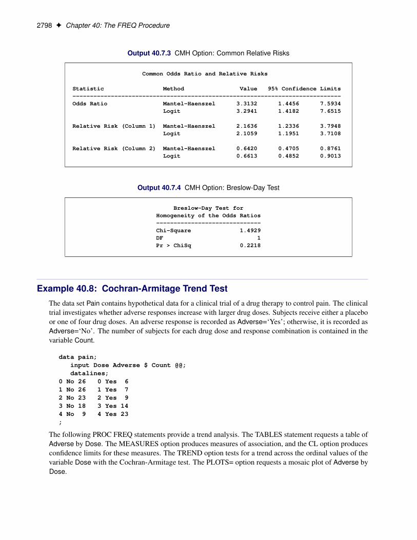
2798 F Chapter 40: The FREQ Procedure
Output 40.7.3 CMH Option: Common Relative Risks
Common Odds Ratio and Relative Risks
Statistic Method Value 95% Confidence Limits-----------------------------------------------------------------------------Odds Ratio Mantel-Haenszel 3.3132 1.4456 7.5934
Logit 3.2941 1.4182 7.6515
Relative Risk (Column 1) Mantel-Haenszel 2.1636 1.2336 3.7948Logit 2.1059 1.1951 3.7108
Relative Risk (Column 2) Mantel-Haenszel 0.6420 0.4705 0.8761Logit 0.6613 0.4852 0.9013
Output 40.7.4 CMH Option: Breslow-Day Test
Breslow-Day Test forHomogeneity of the Odds Ratios------------------------------Chi-Square 1.4929DF 1Pr > ChiSq 0.2218
Example 40.8: Cochran-Armitage Trend TestThe data set Pain contains hypothetical data for a clinical trial of a drug therapy to control pain. The clinicaltrial investigates whether adverse responses increase with larger drug doses. Subjects receive either a placeboor one of four drug doses. An adverse response is recorded as Adverse=‘Yes’; otherwise, it is recorded asAdverse=‘No’. The number of subjects for each drug dose and response combination is contained in thevariable Count.
data pain;input Dose Adverse $ Count @@;datalines;
0 No 26 0 Yes 61 No 26 1 Yes 72 No 23 2 Yes 93 No 18 3 Yes 144 No 9 4 Yes 23;
The following PROC FREQ statements provide a trend analysis. The TABLES statement requests a table ofAdverse by Dose. The MEASURES option produces measures of association, and the CL option producesconfidence limits for these measures. The TREND option tests for a trend across the ordinal values of thevariable Dose with the Cochran-Armitage test. The PLOTS= option requests a mosaic plot of Adverse byDose.

Example 40.8: Cochran-Armitage Trend Test F 2799
The EXACT statement produces exact p-values for this test, and the MAXTIME= option terminates the exactcomputations if they do not complete within 60 seconds. The TEST statement computes an asymptotic testfor Somers’ D.RjC/.
ods graphics on;proc freq data=Pain;
tables Adverse*Dose / trend measures clplots=mosaicplot;
test smdrc;exact trend / maxtime=60;weight Count;title 'Clinical Trial for Treatment of Pain';
run;ods graphics off;
Output 40.8.1 through Output 40.8.4 display the results of the analysis. The “Col Pct” values in Output 40.8.1show the expected increasing trend in the proportion of adverse effects with the increasing dosage (from18.75% to 71.88%). The corresponding mosaic plot (Output 40.8.2) also shows this increasing trend.
Output 40.8.1 Contingency Table
Clinical Trial for Treatment of Pain
The FREQ Procedure
Table of Adverse by Dose
Adverse Dose
Frequency|Percent |Row Pct |Col Pct | 0| 1| 2| 3| 4| Total---------+--------+--------+--------+--------+--------+No | 26 | 26 | 23 | 18 | 9 | 102
| 16.15 | 16.15 | 14.29 | 11.18 | 5.59 | 63.35| 25.49 | 25.49 | 22.55 | 17.65 | 8.82 || 81.25 | 78.79 | 71.88 | 56.25 | 28.13 |
---------+--------+--------+--------+--------+--------+Yes | 6 | 7 | 9 | 14 | 23 | 59
| 3.73 | 4.35 | 5.59 | 8.70 | 14.29 | 36.65| 10.17 | 11.86 | 15.25 | 23.73 | 38.98 || 18.75 | 21.21 | 28.13 | 43.75 | 71.88 |
---------+--------+--------+--------+--------+--------+Total 32 33 32 32 32 161
19.88 20.50 19.88 19.88 19.88 100.00
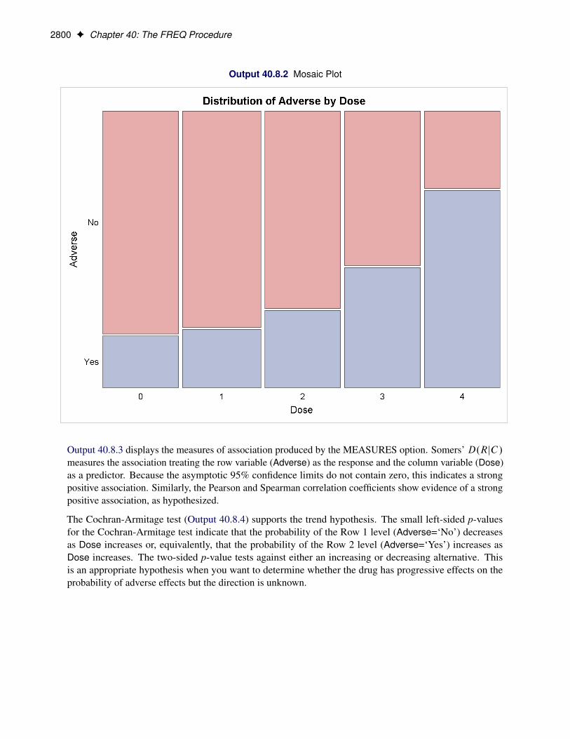
2800 F Chapter 40: The FREQ Procedure
Output 40.8.2 Mosaic Plot
Output 40.8.3 displays the measures of association produced by the MEASURES option. Somers’ D.RjC/measures the association treating the row variable (Adverse) as the response and the column variable (Dose)as a predictor. Because the asymptotic 95% confidence limits do not contain zero, this indicates a strongpositive association. Similarly, the Pearson and Spearman correlation coefficients show evidence of a strongpositive association, as hypothesized.
The Cochran-Armitage test (Output 40.8.4) supports the trend hypothesis. The small left-sided p-valuesfor the Cochran-Armitage test indicate that the probability of the Row 1 level (Adverse=‘No’) decreasesas Dose increases or, equivalently, that the probability of the Row 2 level (Adverse=‘Yes’) increases asDose increases. The two-sided p-value tests against either an increasing or decreasing alternative. Thisis an appropriate hypothesis when you want to determine whether the drug has progressive effects on theprobability of adverse effects but the direction is unknown.
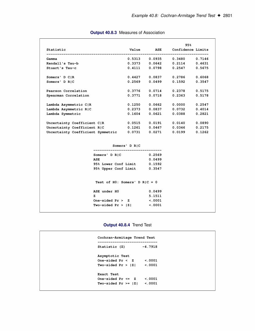
Example 40.8: Cochran-Armitage Trend Test F 2801
Output 40.8.3 Measures of Association
95%Statistic Value ASE Confidence Limits----------------------------------------------------------------------------Gamma 0.5313 0.0935 0.3480 0.7146Kendall's Tau-b 0.3373 0.0642 0.2114 0.4631Stuart's Tau-c 0.4111 0.0798 0.2547 0.5675
Somers' D C|R 0.4427 0.0837 0.2786 0.6068Somers' D R|C 0.2569 0.0499 0.1592 0.3547
Pearson Correlation 0.3776 0.0714 0.2378 0.5175Spearman Correlation 0.3771 0.0718 0.2363 0.5178
Lambda Asymmetric C|R 0.1250 0.0662 0.0000 0.2547Lambda Asymmetric R|C 0.2373 0.0837 0.0732 0.4014Lambda Symmetric 0.1604 0.0621 0.0388 0.2821
Uncertainty Coefficient C|R 0.0515 0.0191 0.0140 0.0890Uncertainty Coefficient R|C 0.1261 0.0467 0.0346 0.2175Uncertainty Coefficient Symmetric 0.0731 0.0271 0.0199 0.1262
Somers' D R|C--------------------------------Somers' D R|C 0.2569ASE 0.049995% Lower Conf Limit 0.159295% Upper Conf Limit 0.3547
Test of H0: Somers' D R|C = 0
ASE under H0 0.0499Z 5.1511One-sided Pr > Z <.0001Two-sided Pr > |Z| <.0001
Output 40.8.4 Trend Test
Cochran-Armitage Trend Test----------------------------Statistic (Z) -4.7918
Asymptotic TestOne-sided Pr < Z <.0001Two-sided Pr > |Z| <.0001
Exact TestOne-sided Pr <= Z <.0001Two-sided Pr >= |Z| <.0001
2802 F Chapter 40: The FREQ Procedure
Example 40.9: Friedman’s Chi-Square TestFriedman’s test is a nonparametric test for treatment differences in a randomized complete block design.Each block of the design might be a subject or a homogeneous group of subjects. If blocks are groups ofsubjects, the number of subjects in each block must equal the number of treatments. Treatments are randomlyassigned to subjects within each block. If there is one subject per block, then the subjects are repeatedlymeasured once under each treatment. The order of treatments is randomized for each subject.
In this setting, Friedman’s test is identical to the ANOVA (row means scores) CMH statistic when the analysisuses rank scores (SCORES=RANK). The three-way table uses subject (or subject group) as the stratifyingvariable, treatment as the row variable, and response as the column variable. PROC FREQ handles ties byassigning midranks to tied response values. If there are multiple subjects per treatment in each block, theANOVA CMH statistic is a generalization of Friedman’s test.
The data set Hypnosis contains data from a study investigating whether hypnosis has the same effect on skinpotential (measured in millivolts) for four emotions (Lehmann and D’Abrera 2006, p. 264). Eight subjectsare asked to display fear, joy, sadness, and calmness under hypnosis. The data are recorded as one observationper subject for each emotion.
data Hypnosis;length Emotion $ 10;input Subject Emotion $ SkinResponse @@;datalines;
1 fear 23.1 1 joy 22.7 1 sadness 22.5 1 calmness 22.62 fear 57.6 2 joy 53.2 2 sadness 53.7 2 calmness 53.13 fear 10.5 3 joy 9.7 3 sadness 10.8 3 calmness 8.34 fear 23.6 4 joy 19.6 4 sadness 21.1 4 calmness 21.65 fear 11.9 5 joy 13.8 5 sadness 13.7 5 calmness 13.36 fear 54.6 6 joy 47.1 6 sadness 39.2 6 calmness 37.07 fear 21.0 7 joy 13.6 7 sadness 13.7 7 calmness 14.88 fear 20.3 8 joy 23.6 8 sadness 16.3 8 calmness 14.8;
In the following PROC FREQ statements, the TABLES statement creates a three-way table stratifiedby Subject and a two-way table; the variables Emotion and SkinResponse form the rows and columnsof each table. The CMH2 option produces the first two Cochran-Mantel-Haenszel statistics, the optionSCORES=RANK specifies that rank scores are used to compute these statistics, and the NOPRINT optionsuppresses the contingency tables. These statements produce Output 40.9.1 and Output 40.9.2.
proc freq data=Hypnosis;tables Subject*Emotion*SkinResponse /
cmh2 scores=rank noprint;run;
proc freq data=Hypnosis;tables Emotion*SkinResponse /
cmh2 scores=rank noprint;run;
Because the CMH statistics in Output 40.9.1 are based on rank scores, the Row Mean Scores Differ statisticis identical to Friedman’s chi-square (Q = 6.45). The p-value of 0.0917 indicates that differences in skinpotential response for different emotions are significant at the 10% level but not at the 5% level.

Example 40.10: Cochran’s Q Test F 2803
When you do not stratify by subject, the Row Mean Scores Differ CMH statistic is identical to a Kruskal-Wallis test and is not significant (p = 0.9038 in Output 40.9.2). Thus, adjusting for subject is critical toreducing the background variation due to subject differences.
Output 40.9.1 CMH Statistics: Stratifying by Subject
Clinical Trial for Treatment of Pain
The FREQ Procedure
Summary Statistics for Emotion by SkinResponseControlling for Subject
Cochran-Mantel-Haenszel Statistics (Based on Rank Scores)
Statistic Alternative Hypothesis DF Value Prob---------------------------------------------------------------
1 Nonzero Correlation 1 0.2400 0.62422 Row Mean Scores Differ 3 6.4500 0.0917
Output 40.9.2 CMH Statistics: No Stratification
Clinical Trial for Treatment of Pain
The FREQ Procedure
Summary Statistics for Emotion by SkinResponse
Cochran-Mantel-Haenszel Statistics (Based on Rank Scores)
Statistic Alternative Hypothesis DF Value Prob---------------------------------------------------------------
1 Nonzero Correlation 1 0.0001 0.99332 Row Mean Scores Differ 3 0.5678 0.9038
Example 40.10: Cochran’s Q TestWhen a binary response is measured several times or under different conditions, Cochran’s Q tests that themarginal probability of a positive response is unchanged across the times or conditions. When there are morethan two response categories, you can use the CATMOD procedure to fit a repeated-measures model.
The data set Drugs contains data for a study of three drugs to treat a chronic disease (Agresti 2002). Forty-sixsubjects receive drugs A, B, and C. The response to each drug is either favorable (‘F’) or unfavorable (‘U’).
proc format;value $ResponseFmt 'F'='Favorable'
'U'='Unfavorable';run;
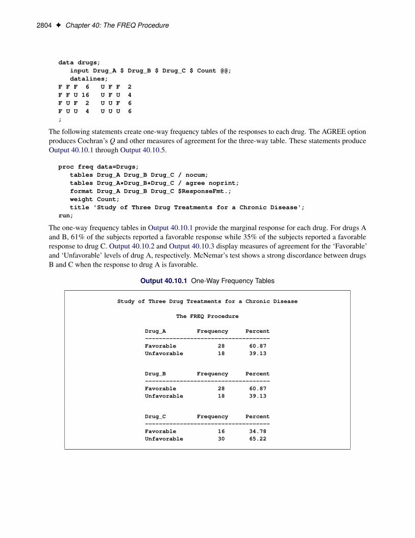
2804 F Chapter 40: The FREQ Procedure
data drugs;input Drug_A $ Drug_B $ Drug_C $ Count @@;datalines;
F F F 6 U F F 2F F U 16 U F U 4F U F 2 U U F 6F U U 4 U U U 6;
The following statements create one-way frequency tables of the responses to each drug. The AGREE optionproduces Cochran’s Q and other measures of agreement for the three-way table. These statements produceOutput 40.10.1 through Output 40.10.5.
proc freq data=Drugs;tables Drug_A Drug_B Drug_C / nocum;tables Drug_A*Drug_B*Drug_C / agree noprint;format Drug_A Drug_B Drug_C $ResponseFmt.;weight Count;title 'Study of Three Drug Treatments for a Chronic Disease';
run;
The one-way frequency tables in Output 40.10.1 provide the marginal response for each drug. For drugs Aand B, 61% of the subjects reported a favorable response while 35% of the subjects reported a favorableresponse to drug C. Output 40.10.2 and Output 40.10.3 display measures of agreement for the ‘Favorable’and ‘Unfavorable’ levels of drug A, respectively. McNemar’s test shows a strong discordance between drugsB and C when the response to drug A is favorable.
Output 40.10.1 One-Way Frequency Tables
Study of Three Drug Treatments for a Chronic Disease
The FREQ Procedure
Drug_A Frequency Percent------------------------------------Favorable 28 60.87Unfavorable 18 39.13
Drug_B Frequency Percent------------------------------------Favorable 28 60.87Unfavorable 18 39.13
Drug_C Frequency Percent------------------------------------Favorable 16 34.78Unfavorable 30 65.22
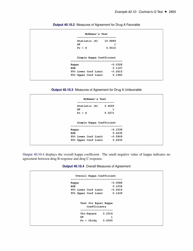
Example 40.10: Cochran’s Q Test F 2805
Output 40.10.2 Measures of Agreement for Drug A Favorable
McNemar's Test------------------------Statistic (S) 10.8889DF 1Pr > S 0.0010
Simple Kappa Coefficient--------------------------------Kappa -0.0328ASE 0.116795% Lower Conf Limit -0.261595% Upper Conf Limit 0.1960
Output 40.10.3 Measures of Agreement for Drug A Unfavorable
McNemar's Test-----------------------Statistic (S) 0.4000DF 1Pr > S 0.5271
Simple Kappa Coefficient--------------------------------Kappa -0.1538ASE 0.223095% Lower Conf Limit -0.590995% Upper Conf Limit 0.2832
Output 40.10.4 displays the overall kappa coefficient. The small negative value of kappa indicates noagreement between drug B response and drug C response.
Output 40.10.4 Overall Measures of Agreement
Overall Kappa Coefficient--------------------------------Kappa -0.0588ASE 0.103495% Lower Conf Limit -0.261595% Upper Conf Limit 0.1439
Test for Equal KappaCoefficients
--------------------Chi-Square 0.2314DF 1Pr > ChiSq 0.6305
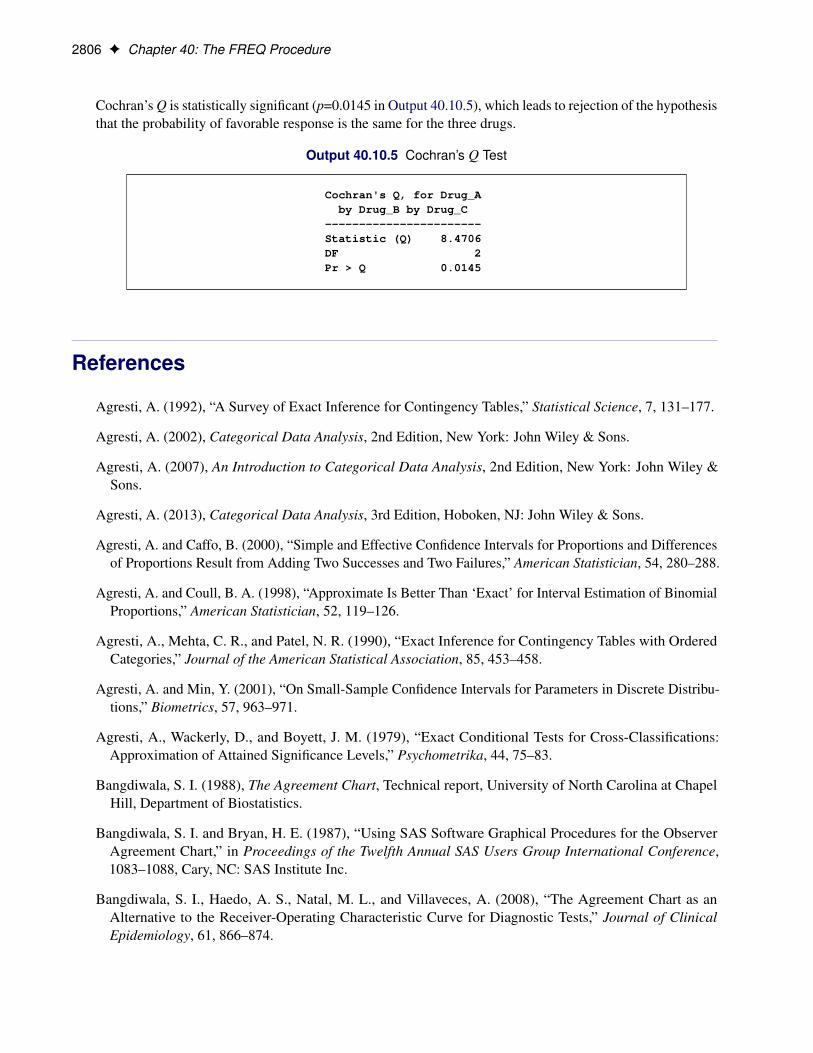
2806 F Chapter 40: The FREQ Procedure
Cochran’s Q is statistically significant (p=0.0145 in Output 40.10.5), which leads to rejection of the hypothesisthat the probability of favorable response is the same for the three drugs.
Output 40.10.5 Cochran’s Q Test
Cochran's Q, for Drug_Aby Drug_B by Drug_C
-----------------------Statistic (Q) 8.4706DF 2Pr > Q 0.0145
References
Agresti, A. (1992), “A Survey of Exact Inference for Contingency Tables,” Statistical Science, 7, 131–177.
Agresti, A. (2002), Categorical Data Analysis, 2nd Edition, New York: John Wiley & Sons.
Agresti, A. (2007), An Introduction to Categorical Data Analysis, 2nd Edition, New York: John Wiley &Sons.
Agresti, A. (2013), Categorical Data Analysis, 3rd Edition, Hoboken, NJ: John Wiley & Sons.
Agresti, A. and Caffo, B. (2000), “Simple and Effective Confidence Intervals for Proportions and Differencesof Proportions Result from Adding Two Successes and Two Failures,” American Statistician, 54, 280–288.
Agresti, A. and Coull, B. A. (1998), “Approximate Is Better Than ‘Exact’ for Interval Estimation of BinomialProportions,” American Statistician, 52, 119–126.
Agresti, A., Mehta, C. R., and Patel, N. R. (1990), “Exact Inference for Contingency Tables with OrderedCategories,” Journal of the American Statistical Association, 85, 453–458.
Agresti, A. and Min, Y. (2001), “On Small-Sample Confidence Intervals for Parameters in Discrete Distribu-tions,” Biometrics, 57, 963–971.
Agresti, A., Wackerly, D., and Boyett, J. M. (1979), “Exact Conditional Tests for Cross-Classifications:Approximation of Attained Significance Levels,” Psychometrika, 44, 75–83.
Bangdiwala, S. I. (1988), The Agreement Chart, Technical report, University of North Carolina at ChapelHill, Department of Biostatistics.
Bangdiwala, S. I. and Bryan, H. E. (1987), “Using SAS Software Graphical Procedures for the ObserverAgreement Chart,” in Proceedings of the Twelfth Annual SAS Users Group International Conference,1083–1088, Cary, NC: SAS Institute Inc.
Bangdiwala, S. I., Haedo, A. S., Natal, M. L., and Villaveces, A. (2008), “The Agreement Chart as anAlternative to the Receiver-Operating Characteristic Curve for Diagnostic Tests,” Journal of ClinicalEpidemiology, 61, 866–874.

References F 2807
Barker, L., Rolka, H., Rolka, D., and Brown, C. (2001), “Equivalence Testing for Binomial Random Variables:Which Test to Use?” American Statistician, 55, 279–287.
Barnard, G. A. (1945), “A New Test for 2 � 2 Tables,” Nature, 156, 177.
Barnard, G. A. (1947), “Significance Tests for 2 � 2 Tables,” Biometrika, 34, 123–138.
Barnard, G. A. (1949), “Statistical Inference,” Journal of the Royal Statistical Society, Series B, 11, 115–139.
Berger, J. O. (1985), Statistical Decision Theory and Bayesian Analysis, 2nd Edition, New York: Springer-Verlag.
Birch, M. W. (1965), “The Detection of Partial Association, Part 2: The General Case,” Journal of the RoyalStatistical Society, Series B, 27, 111–124.
Bishop, Y. M. M., Fienberg, S. E., and Holland, P. W. (1975), Discrete Multivariate Analysis: Theory andPractice, Cambridge, MA: MIT Press.
Bowker, A. H. (1948), “Bowker’s Test for Symmetry,” Journal of the American Statistical Association, 43,572–574.
Breslow, N. E. (1996), “Statistics in Epidemiology: The Case-Control Study,” Journal of the AmericanStatistical Association, 91, 14–26.
Breslow, N. E. and Day, N. E. (1980), The Analysis of Case-Control Studies, Statistical Methods in CancerResearch, IARC Scientific Publications, vol. 1, no. 32, Lyon: International Agency for Research on Cancer.
Breslow, N. E. and Day, N. E. (1987), The Design and Analysis of Cohort Studies, Statistical Methods inCancer Research, IARC Scientific Publications, vol. 2, no. 82, Lyon: International Agency for Researchon Cancer.
Bross, I. D. J. (1958), “How to Use Ridit Analysis,” Biometrics, 14, 18–38.
Brown, L. D., Cai, T. T., and DasGupta, A. (2001), “Interval Estimation for a Binomial Proportion,” StatisticalScience, 16, 101–133.
Brown, M. B. and Benedetti, J. K. (1977), “Sampling Behavior of Tests for Correlation in Two-WayContingency Tables,” Journal of the American Statistical Association, 72, 309–315.
Chan, I. S. F. (1998), “Exact Tests of Equivalence and Efficacy with a Non-zero Lower Bound for ComparativeStudies,” Statistics in Medicine, 17, 1403–1413.
Chan, I. S. F. (2003), “Proving Non-inferiority or Equivalence of Two Treatments with DichotomousEndpoints Using Exact Methods,” Statistical Methods in Medical Research, 12, 37–58.
Chan, I. S. F. and Zhang, Z. (1999), “Test-Based Exact Confidence Intervals for the Difference of TwoBinomial Proportions,” Biometrics, 55, 1202–1209.
Chow, S.-C., Shao, J., and Wang, H. (2003), Sample Size Calculations in Clinical Research, Boca Raton, FL:CRC Press.
Cicchetti, D. V. and Allison, T. (1971), “A New Procedure for Assessing Reliability of Scoring EEG SleepRecordings,” American Journal of EEG Technology, 11, 101–109.
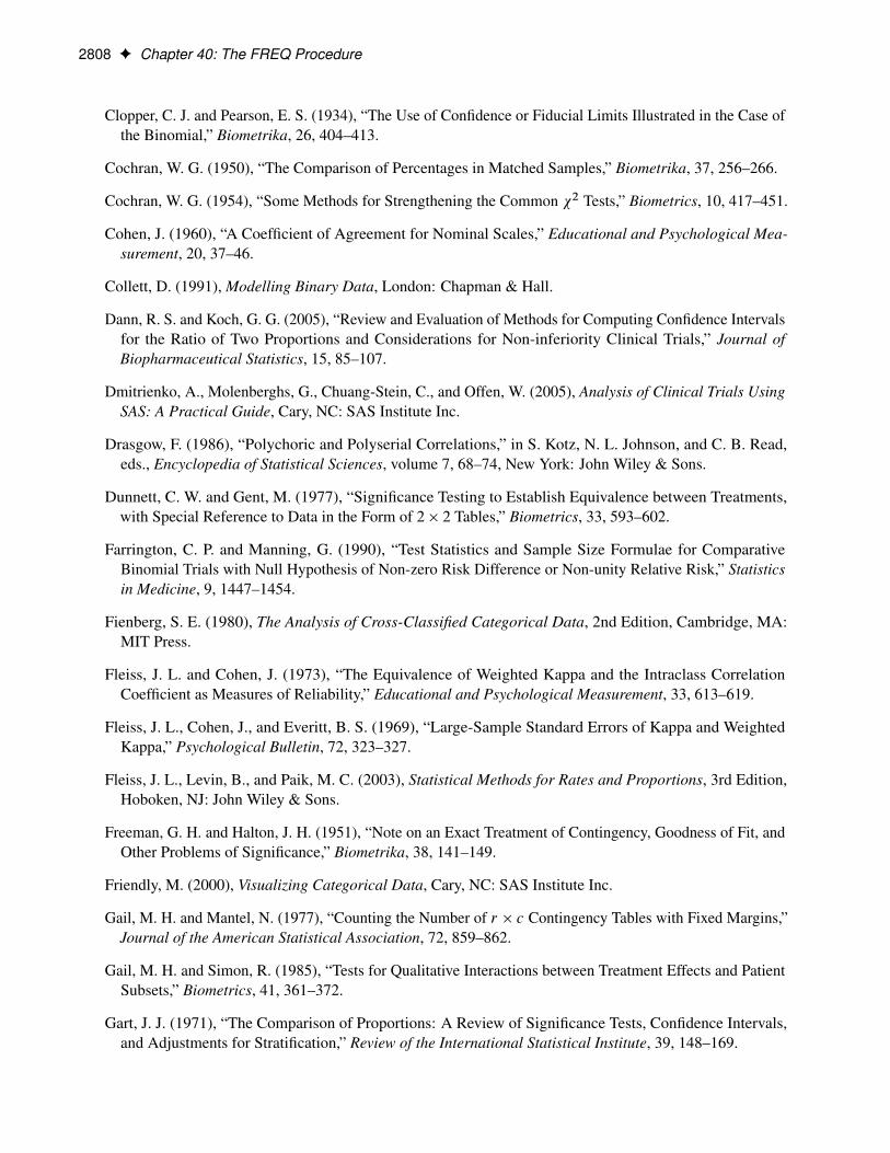
2808 F Chapter 40: The FREQ Procedure
Clopper, C. J. and Pearson, E. S. (1934), “The Use of Confidence or Fiducial Limits Illustrated in the Case ofthe Binomial,” Biometrika, 26, 404–413.
Cochran, W. G. (1950), “The Comparison of Percentages in Matched Samples,” Biometrika, 37, 256–266.
Cochran, W. G. (1954), “Some Methods for Strengthening the Common �2 Tests,” Biometrics, 10, 417–451.
Cohen, J. (1960), “A Coefficient of Agreement for Nominal Scales,” Educational and Psychological Mea-surement, 20, 37–46.
Collett, D. (1991), Modelling Binary Data, London: Chapman & Hall.
Dann, R. S. and Koch, G. G. (2005), “Review and Evaluation of Methods for Computing Confidence Intervalsfor the Ratio of Two Proportions and Considerations for Non-inferiority Clinical Trials,” Journal ofBiopharmaceutical Statistics, 15, 85–107.
Dmitrienko, A., Molenberghs, G., Chuang-Stein, C., and Offen, W. (2005), Analysis of Clinical Trials UsingSAS: A Practical Guide, Cary, NC: SAS Institute Inc.
Drasgow, F. (1986), “Polychoric and Polyserial Correlations,” in S. Kotz, N. L. Johnson, and C. B. Read,eds., Encyclopedia of Statistical Sciences, volume 7, 68–74, New York: John Wiley & Sons.
Dunnett, C. W. and Gent, M. (1977), “Significance Testing to Establish Equivalence between Treatments,with Special Reference to Data in the Form of 2 � 2 Tables,” Biometrics, 33, 593–602.
Farrington, C. P. and Manning, G. (1990), “Test Statistics and Sample Size Formulae for ComparativeBinomial Trials with Null Hypothesis of Non-zero Risk Difference or Non-unity Relative Risk,” Statisticsin Medicine, 9, 1447–1454.
Fienberg, S. E. (1980), The Analysis of Cross-Classified Categorical Data, 2nd Edition, Cambridge, MA:MIT Press.
Fleiss, J. L. and Cohen, J. (1973), “The Equivalence of Weighted Kappa and the Intraclass CorrelationCoefficient as Measures of Reliability,” Educational and Psychological Measurement, 33, 613–619.
Fleiss, J. L., Cohen, J., and Everitt, B. S. (1969), “Large-Sample Standard Errors of Kappa and WeightedKappa,” Psychological Bulletin, 72, 323–327.
Fleiss, J. L., Levin, B., and Paik, M. C. (2003), Statistical Methods for Rates and Proportions, 3rd Edition,Hoboken, NJ: John Wiley & Sons.
Freeman, G. H. and Halton, J. H. (1951), “Note on an Exact Treatment of Contingency, Goodness of Fit, andOther Problems of Significance,” Biometrika, 38, 141–149.
Friendly, M. (2000), Visualizing Categorical Data, Cary, NC: SAS Institute Inc.
Gail, M. H. and Mantel, N. (1977), “Counting the Number of r � c Contingency Tables with Fixed Margins,”Journal of the American Statistical Association, 72, 859–862.
Gail, M. H. and Simon, R. (1985), “Tests for Qualitative Interactions between Treatment Effects and PatientSubsets,” Biometrics, 41, 361–372.
Gart, J. J. (1971), “The Comparison of Proportions: A Review of Significance Tests, Confidence Intervals,and Adjustments for Stratification,” Review of the International Statistical Institute, 39, 148–169.
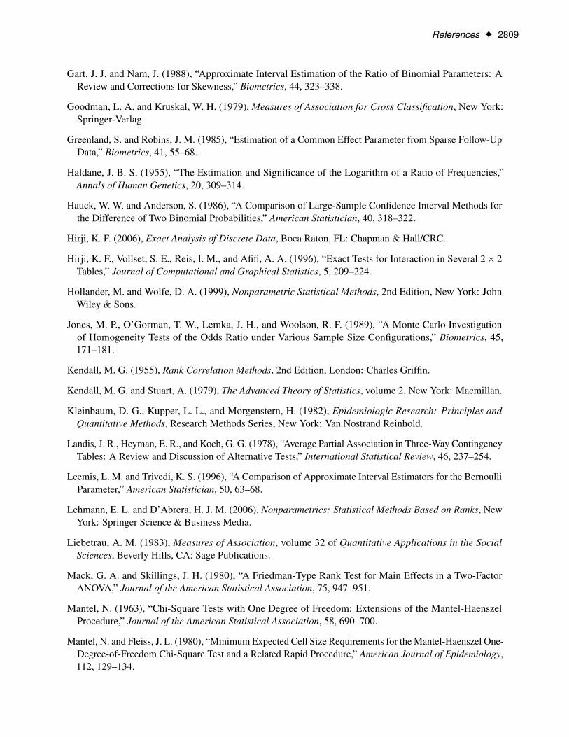
References F 2809
Gart, J. J. and Nam, J. (1988), “Approximate Interval Estimation of the Ratio of Binomial Parameters: AReview and Corrections for Skewness,” Biometrics, 44, 323–338.
Goodman, L. A. and Kruskal, W. H. (1979), Measures of Association for Cross Classification, New York:Springer-Verlag.
Greenland, S. and Robins, J. M. (1985), “Estimation of a Common Effect Parameter from Sparse Follow-UpData,” Biometrics, 41, 55–68.
Haldane, J. B. S. (1955), “The Estimation and Significance of the Logarithm of a Ratio of Frequencies,”Annals of Human Genetics, 20, 309–314.
Hauck, W. W. and Anderson, S. (1986), “A Comparison of Large-Sample Confidence Interval Methods forthe Difference of Two Binomial Probabilities,” American Statistician, 40, 318–322.
Hirji, K. F. (2006), Exact Analysis of Discrete Data, Boca Raton, FL: Chapman & Hall/CRC.
Hirji, K. F., Vollset, S. E., Reis, I. M., and Afifi, A. A. (1996), “Exact Tests for Interaction in Several 2 � 2Tables,” Journal of Computational and Graphical Statistics, 5, 209–224.
Hollander, M. and Wolfe, D. A. (1999), Nonparametric Statistical Methods, 2nd Edition, New York: JohnWiley & Sons.
Jones, M. P., O’Gorman, T. W., Lemka, J. H., and Woolson, R. F. (1989), “A Monte Carlo Investigationof Homogeneity Tests of the Odds Ratio under Various Sample Size Configurations,” Biometrics, 45,171–181.
Kendall, M. G. (1955), Rank Correlation Methods, 2nd Edition, London: Charles Griffin.
Kendall, M. G. and Stuart, A. (1979), The Advanced Theory of Statistics, volume 2, New York: Macmillan.
Kleinbaum, D. G., Kupper, L. L., and Morgenstern, H. (1982), Epidemiologic Research: Principles andQuantitative Methods, Research Methods Series, New York: Van Nostrand Reinhold.
Landis, J. R., Heyman, E. R., and Koch, G. G. (1978), “Average Partial Association in Three-Way ContingencyTables: A Review and Discussion of Alternative Tests,” International Statistical Review, 46, 237–254.
Leemis, L. M. and Trivedi, K. S. (1996), “A Comparison of Approximate Interval Estimators for the BernoulliParameter,” American Statistician, 50, 63–68.
Lehmann, E. L. and D’Abrera, H. J. M. (2006), Nonparametrics: Statistical Methods Based on Ranks, NewYork: Springer Science & Business Media.
Liebetrau, A. M. (1983), Measures of Association, volume 32 of Quantitative Applications in the SocialSciences, Beverly Hills, CA: Sage Publications.
Mack, G. A. and Skillings, J. H. (1980), “A Friedman-Type Rank Test for Main Effects in a Two-FactorANOVA,” Journal of the American Statistical Association, 75, 947–951.
Mantel, N. (1963), “Chi-Square Tests with One Degree of Freedom: Extensions of the Mantel-HaenszelProcedure,” Journal of the American Statistical Association, 58, 690–700.
Mantel, N. and Fleiss, J. L. (1980), “Minimum Expected Cell Size Requirements for the Mantel-Haenszel One-Degree-of-Freedom Chi-Square Test and a Related Rapid Procedure,” American Journal of Epidemiology,112, 129–134.

2810 F Chapter 40: The FREQ Procedure
Mantel, N. and Haenszel, W. (1959), “Statistical Aspects of Analysis of Data from Retrospective Studies ofDisease,” Journal of the National Cancer Institute, 22, 719–748.
Margolin, B. H. (1988), “Test for Trend in Proportions,” in S. Kotz, N. L. Johnson, and C. B. Read, eds.,Encyclopedia of Statistical Sciences, volume 9, 334–336, New York: John Wiley & Sons.
McNemar, Q. (1947), “Note on the Sampling Error of the Difference between Correlated Proportions orPercentages,” Psychometrika, 12, 153–157.
Mee, R. W. (1984), “Confidence Bounds for the Difference between Two Probabilities,” Biometrics, 40,1175–1176.
Mehta, C. R. and Patel, N. R. (1983), “A Network Algorithm for Performing Fisher’s Exact Test in r � cContingency Tables,” Journal of the American Statistical Association, 78, 427–434.
Mehta, C. R., Patel, N. R., and Gray, R. J. (1985), “Computing an Exact Confidence Interval for the CommonOdds Ratio in Several 2�2 Contingency Tables,” Journal of American Statistical Association, 80, 969–973.
Mehta, C. R., Patel, N. R., and Senchaudhuri, P. (1991), “Exact Stratified Linear Rank Tests for Binary Data,”in E. M. Keramidas, ed., Computing Science and Statistics: Proceedings of the 23rd Symposium on theInterface, 200–207, Fairfax Station, VA: Interface Foundation.
Mehta, C. R., Patel, N. R., and Tsiatis, A. A. (1984), “Exact Significance Testing to Establish TreatmentEquivalence with Ordered Categorical Data,” Biometrics, 40, 819–825.
Mehta, C. R. and Senchaudhuri, P. (2003), “Conditional versus Unconditional Exact Tests for ComparingTwo Binomials,” .
Miettinen, O. S. (1985), Theoretical Epidemiology: Principles of Occurrence in Research Medicine, NewYork: John Wiley & Sons.
Miettinen, O. S. and Nurminen, M. M. (1985), “Comparative Analysis of Two Rates,” Statistics in Medicine,4, 213–226.
Newcombe, R. G. (1998a), “Interval Estimation for the Difference between Independent Proportions:Comparison of Eleven Methods,” Statistics in Medicine, 17, 873–890.
Newcombe, R. G. (1998b), “Two-Sided Confidence Intervals for the Single Proportion: Comparison of SevenMethods,” Statistics in Medicine, 17, 857–872.
Newcombe, R. G. and Nurminen, M. M. (2011), “In Defence of Score Intervals for Proportions and TheirDifferences,” Communications in Statistics—Theory and Methods, 40, 1271–1282.
Olsson, U. (1979), “Maximum Likelihood Estimation of the Polychoric Correlation Coefficient,” Psychome-trika, 12, 443–460.
Pirie, W. (1983), “Jonckheere Tests for Ordered Alternatives,” in S. Kotz, N. L. Johnson, and C. B. Read,eds., Encyclopedia of Statistical Sciences, volume 4, 315–318, New York: John Wiley & Sons.
Radlow, R. and Alf, E. F. (1975), “An Alternate Multinomial Assessment of the Accuracy of the Chi-SquareTest of Goodness of Fit,” Journal of the American Statistical Association, 70, 811–813.
Robins, J. M., Breslow, N., and Greenland, S. (1986), “Estimators of the Mantel-Haenszel Variance Consistentin Both Sparse Data and Large-Strata Limiting Models,” Biometrics, 42, 311–323.

References F 2811
Santner, T. J., Pradhan, V., Senchaudhuri, P., Mehta, C. R., and Tamhane, A. (2007), “Small-SampleComparisons of Confidence Intervals for the Difference of Two Independent Binomial Proportions,”Computational Statistics and Data Analysis, 51, 5791–5799.
Santner, T. J. and Snell, M. K. (1980), “Small-Sample Confidence Intervals for p1 � p2 and p1=p2 in 2 � 2Contingency Tables,” Journal of the American Statistical Association, 75, 386–394.
Sato, T. (1989), “On the Variance Estimator of the Mantel-Haenszel Risk Difference,” Biometrics, 45,1323–1324, letter to the editor.
Schuirmann, D. J. (1987), “A Comparison of the Two One-Sided Tests Procedure and the Power Approach forAssessing the Equivalence of Average Bioavailability,” Journal of Pharmacokinetics and Biopharmaceutics,15, 657–680.
Schuirmann, D. J. (1999), “Confidence Interval Methods for Bioequivalence Testing with Binomial End-points,” in Proceedings of the Biopharmaceutical Section, 227–232, Alexandria, VA: American StatisticalAssociation.
Silvapulle, M. J. (2001), “Tests against Qualitative Interaction: Exact Critical Values and Robust Tests,”Biometrics, 57, 1157–1165.
Snedecor, G. W. and Cochran, W. G. (1989), Statistical Methods, 8th Edition, Ames: Iowa State UniversityPress.
Somers, R. H. (1962), “A New Asymmetric Measure of Association for Ordinal Variables,” AmericanSociological Review, 27, 799–811.
Stokes, M. E., Davis, C. S., and Koch, G. G. (2012), Categorical Data Analysis Using SAS, 3rd Edition, Cary,NC: SAS Institute Inc.
Suissa, S. and Shuster, J. J. (1985), “Exact Unconditional Sample Sizes for the 2� 2 Binomial Trial,” Journalof the Royal Statistical Society, Series A, 148, 317–327.
Tarone, R. E. (1985), “On Heterogeneity Tests Based on Efficient Scores,” Biometrika, 72, 1, 91–95.
Theil, H. (1972), Statistical Decomposition Analysis, Amsterdam: North-Holland.
Thomas, D. G. (1971), “Algorithm AS-36: Exact Confidence Limits for the Odds Ratio in a 2 � 2 Table,”Applied Statistics, 20, 105–110.
Valz, P. D. and Thompson, M. E. (1994), “Exact Inference for Kendall’s S and Spearman’s � with Extensionsto Fisher’s Exact Test in r � c Contingency Tables,” Journal of Computational and Graphical Statistics, 3,459–472.
van Elteren, P. H. (1960), “On the Combination of Independent Two-Sample Tests of Wilcoxon,” Bulletin ofthe International Statistical Institute, 37, 351–361.
Vollset, S. E., Hirji, K. F., and Elashoff, R. M. (1991), “Fast Computation of Exact Confidence Limits forthe Common Odds Ratio in a Series of 2 � 2 Tables,” Journal of the American Statistical Association, 86,404–409.
Wilson, E. B. (1927), “Probable Inference, the Law of Succession, and Statistical Inference,” Journal of theAmerican Statistical Association, 22, 209–212.

2812 F Chapter 40: The FREQ Procedure
Woolf, B. (1955), “On Estimating the Relationship between Blood Group and Disease,” Annals of HumanGenetics, 19, 251–253.
Zelen, M. (1971), “The Analysis of Several 2 � 2 Contingency Tables,” Biometrika, 58, 129–137.

Subject Index
adjusted odds ratioFREQ procedure, 2752
adjusted relative risksFREQ procedure, 2753
agreement plotsFREQ procedure, 2634
agreement, measures ofFREQ procedure, 2743
Agresti-Caffo confidence limitsrisk difference (FREQ), 2727
Agresti-Coull confidence limitsproportions (FREQ), 2719
ANOVA (row mean scores) statisticMantel-Haenszel (FREQ), 2750
association, measures ofFREQ procedure, 2709
bar chartsFREQ procedure, 2686
Barnard’s testFREQ procedure, 2735
binomial proportionsClopper-Pearson test (FREQ), 2722confidence limits (FREQ), 2719equivalence tests (FREQ), 2724exact test (FREQ), 2722FREQ procedure, 2719noninferiority tests (FREQ), 2722superiority tests (FREQ), 2723tests (FREQ), 2721TOST (FREQ), 2724
Bowker’s test of symmetryFREQ procedure, 2743, 2744
Breslow-Day testFREQ procedure, 2753Tarone’s adjustment (FREQ), 2753
case-control studiesodds ratio (FREQ), 2737
categorical data analysisFREQ procedure, 2622
cell count dataexample (FREQ), 2778FREQ procedure, 2697
chi-square goodness-of-fit testFREQ procedure, 2704
chi-square testsFREQ procedure, 2704
Cicchetti-Allison weights
kappa coefficient (FREQ), 2746Clopper-Pearson confidence limits
proportions (FREQ), 2720Cochran’s Q test
FREQ procedure, 2743, 2747Cochran-Armitage test for trend
FREQ procedure, 2740Cochran-Mantel-Haenszel statistics
FREQ procedure, 2748cohort studies
relative risks (FREQ), 2739common odds ratio
exact confidence limits (FREQ), 2754exact test (FREQ), 2754logit (FREQ), 2752Mantel-Haenszel (FREQ), 2752
common relative riskslogit (FREQ), 2753Mantel-Haenszel (FREQ), 2753
concordant observationsFREQ procedure, 2709
confidence limitsexact (FREQ), 2637measures of association (FREQ), 2710proportions (FREQ), 2719
contingency coefficientFREQ procedure, 2709
contingency tablesFREQ procedure, 2622, 2656
continuity-adjusted chi-square testFREQ procedure, 2707
correlation statisticMantel-Haenszel (FREQ), 2749
Cramér’s V statisticFREQ procedure, 2709
crosstabulation tablesFREQ procedure, 2622, 2656, 2767
discordant observationsFREQ procedure, 2709
dot plotsFREQ procedure, 2686, 2781
equivalence testsbinomial proportions (FREQ), 2724risk difference (FREQ), 2733
exact confidence limitsodds ratio (FREQ), 2738proportion difference (FREQ), 2734
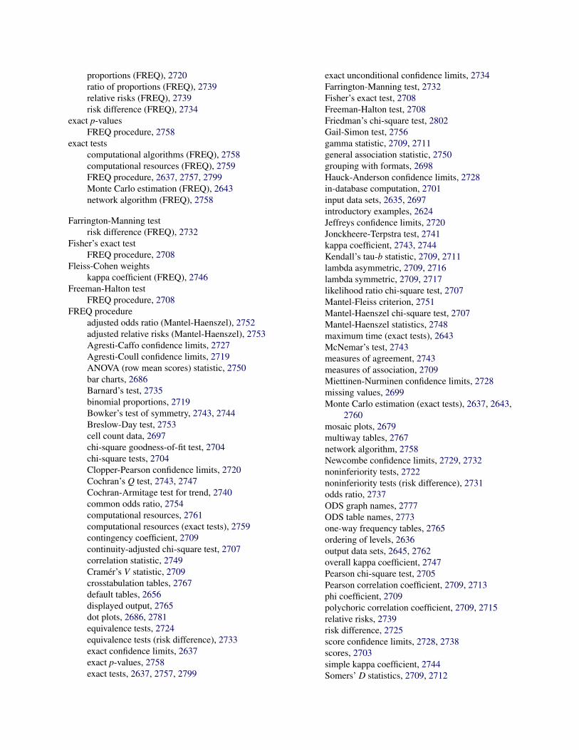
proportions (FREQ), 2720ratio of proportions (FREQ), 2739relative risks (FREQ), 2739risk difference (FREQ), 2734
exact p-valuesFREQ procedure, 2758
exact testscomputational algorithms (FREQ), 2758computational resources (FREQ), 2759FREQ procedure, 2637, 2757, 2799Monte Carlo estimation (FREQ), 2643network algorithm (FREQ), 2758
Farrington-Manning testrisk difference (FREQ), 2732
Fisher’s exact testFREQ procedure, 2708
Fleiss-Cohen weightskappa coefficient (FREQ), 2746
Freeman-Halton testFREQ procedure, 2708
FREQ procedureadjusted odds ratio (Mantel-Haenszel), 2752adjusted relative risks (Mantel-Haenszel), 2753Agresti-Caffo confidence limits, 2727Agresti-Coull confidence limits, 2719ANOVA (row mean scores) statistic, 2750bar charts, 2686Barnard’s test, 2735binomial proportions, 2719Bowker’s test of symmetry, 2743, 2744Breslow-Day test, 2753cell count data, 2697chi-square goodness-of-fit test, 2704chi-square tests, 2704Clopper-Pearson confidence limits, 2720Cochran’s Q test, 2743, 2747Cochran-Armitage test for trend, 2740common odds ratio, 2754computational resources, 2761computational resources (exact tests), 2759contingency coefficient, 2709continuity-adjusted chi-square test, 2707correlation statistic, 2749Cramér’s V statistic, 2709crosstabulation tables, 2767default tables, 2656displayed output, 2765dot plots, 2686, 2781equivalence tests, 2724equivalence tests (risk difference), 2733exact confidence limits, 2637exact p-values, 2758exact tests, 2637, 2757, 2799
exact unconditional confidence limits, 2734Farrington-Manning test, 2732Fisher’s exact test, 2708Freeman-Halton test, 2708Friedman’s chi-square test, 2802Gail-Simon test, 2756gamma statistic, 2709, 2711general association statistic, 2750grouping with formats, 2698Hauck-Anderson confidence limits, 2728in-database computation, 2701input data sets, 2635, 2697introductory examples, 2624Jeffreys confidence limits, 2720Jonckheere-Terpstra test, 2741kappa coefficient, 2743, 2744Kendall’s tau-b statistic, 2709, 2711lambda asymmetric, 2709, 2716lambda symmetric, 2709, 2717likelihood ratio chi-square test, 2707Mantel-Fleiss criterion, 2751Mantel-Haenszel chi-square test, 2707Mantel-Haenszel statistics, 2748maximum time (exact tests), 2643McNemar’s test, 2743measures of agreement, 2743measures of association, 2709Miettinen-Nurminen confidence limits, 2728missing values, 2699Monte Carlo estimation (exact tests), 2637, 2643,
2760mosaic plots, 2679multiway tables, 2767network algorithm, 2758Newcombe confidence limits, 2729, 2732noninferiority tests, 2722noninferiority tests (risk difference), 2731odds ratio, 2737ODS graph names, 2777ODS table names, 2773one-way frequency tables, 2765ordering of levels, 2636output data sets, 2645, 2762overall kappa coefficient, 2747Pearson chi-square test, 2705Pearson correlation coefficient, 2709, 2713phi coefficient, 2709polychoric correlation coefficient, 2709, 2715relative risks, 2739risk difference, 2725score confidence limits, 2728, 2738scores, 2703simple kappa coefficient, 2744Somers’ D statistics, 2709, 2712

Spearman rank correlation coefficient, 2709, 2714standardized residuals, 2705Stuart’s tau-c statistic, 2709, 2712superiority tests, 2723superiority tests (risk difference), 2733tetrachoric correlation coefficient, 2715uncertainty coefficients, 2709, 2718Wald confidence limits (risk difference), 2730weighted kappa coefficient, 2743, 2745Wilson confidence limits, 2720Yule’s Q statistic, 2711Zelen’s exact test, 2754
frequency plotsFREQ procedure, 2626
frequency tablesFREQ procedure, 2622, 2656one-way (FREQ), 2765
Friedman’s chi-square testFREQ procedure, 2802
Gail-Simon testFREQ procedure, 2756
gamma statisticFREQ procedure, 2709, 2711
general association statisticMantel-Haenszel (FREQ), 2750
Hauck-Anderson confidence limitsrisk difference (FREQ), 2728
hypothesis testsexact (FREQ), 2637
in-database computationFREQ procedure, 2701
Jeffreys confidence limitsproportions (FREQ), 2720
Jonckheere-Terpstra testFREQ procedure, 2741
kappa coefficientFREQ procedure, 2743, 2744weights (FREQ), 2746
Kendall’s tau-b statisticFREQ procedure, 2709, 2711
lambda asymmetricFREQ procedure, 2709, 2716
lambda symmetricFREQ procedure, 2709, 2717
likelihood ratio chi-square testFREQ procedure, 2707
Mantel-Fleiss criterionFREQ procedure, 2751
Mantel-Haenszel chi-square testFREQ procedure, 2707
Mantel-Haenszel statisticsANOVA (row mean scores) statistic (FREQ),
2750correlation statistic (FREQ), 2749FREQ procedure, 2748general association statistic (FREQ), 2750Mantel-Fleiss criterion (FREQ), 2751
McNemar’s testFREQ procedure, 2743
measures of associationexact tests (FREQ), 2711tests (FREQ), 2710
Mehta-Patel network algorithmexact tests (FREQ), 2758
Miettinen-Nurminen confidence limitsrisk difference (FREQ), 2728
missing valuesFREQ procedure, 2699
modified ridit scoresFREQ procedure, 2703
Monte Carlo estimationexact tests (FREQ), 2637, 2643, 2760
mosaic plotsFREQ procedure, 2679
multiway tablesFREQ procedure, 2622, 2656, 2767
network algorithmexact tests (FREQ), 2758
Newcombe confidence limitsrisk difference (FREQ), 2729, 2732
noninferiority testsbinomial proportions (FREQ), 2722risk difference (FREQ), 2731
odds ratioBreslow-Day test (FREQ), 2753case-control studies (FREQ), 2737exact confidence limits (FREQ), 2738FREQ procedure, 2737logit adjusted (FREQ), 2752Mantel-Haenszel adjusted (FREQ), 2752Zelen’s exact test (FREQ), 2754
ODS graph namesFREQ procedure, 2777
Pearson chi-square testFREQ procedure, 2705
Pearson correlation coefficientFREQ procedure, 2709, 2713
phi coefficientFREQ procedure, 2709
polychoric correlation coefficient

FREQ procedure, 2709, 2715proportion difference
FREQ procedure, 2725proportions, see binomial proportions (FREQ)
rank scoresFREQ procedure, 2703
relative riskscohort studies (FREQ), 2739exact confidence limits (FREQ), 2739FREQ procedure, 2739logit adjusted (FREQ), 2753Mantel-Haenszel adjusted (FREQ), 2753
ridit scoresFREQ procedure, 2703
risk differenceconfidence limits (FREQ), 2727equivalence tests (FREQ), 2733exact confidence limits (FREQ), 2734FREQ procedure, 2725noninferiority tests (FREQ), 2731superiority tests (FREQ), 2733tests (FREQ), 2730TOST (FREQ), 2733
risks, see also binomial proportions (FREQ)FREQ procedure, 2725
row mean scores statisticMantel-Haenszel (FREQ), 2750
score confidence limitsodds ratio (FREQ), 2738risk difference (FREQ), 2728
Somers’ D statisticsFREQ procedure, 2709, 2712
Spearman rank correlation coefficientFREQ procedure, 2709, 2714
standardized residualsFREQ procedure, 2705
stratified analysisFREQ procedure, 2622, 2656
Stuart’s tau-c statisticFREQ procedure, 2709, 2712
superiority testsbinomial proportions (FREQ), 2723risk difference (FREQ), 2733
table scoresFREQ procedure, 2703
tablescontingency (FREQ), 2622crosstabulation (FREQ), 2622, 2767multiway (FREQ), 2622, 2767one-way frequency (FREQ), 2622, 2765
Tarone’s adjustmentBreslow-Day test (FREQ), 2753
tetrachoric correlation coefficientFREQ procedure, 2715
TOSTequivalence tests (FREQ), 2724, 2733
trend testFREQ procedure, 2740
uncertainty coefficientsFREQ procedure, 2709, 2718
Wald confidence limitsrisk difference (FREQ), 2730
weighted kappa coefficientFREQ procedure, 2743, 2745
Wilson confidence limitsproportions (FREQ), 2720
Yule’s Q statisticFREQ procedure, 2711
Zelen’s testequal odds ratios (FREQ), 2754
zeros, structural and randomagreement statistics (FREQ), 2747
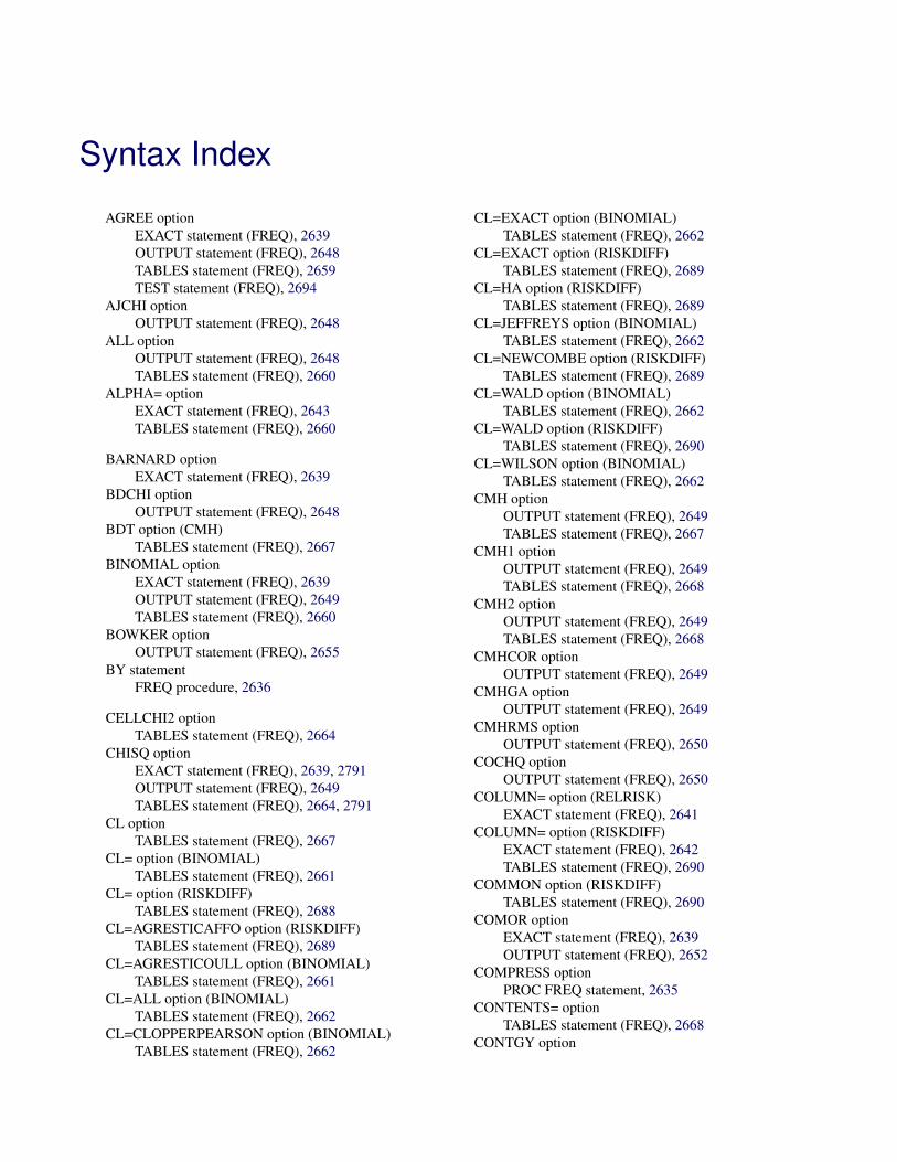
Syntax Index
AGREE optionEXACT statement (FREQ), 2639OUTPUT statement (FREQ), 2648TABLES statement (FREQ), 2659TEST statement (FREQ), 2694
AJCHI optionOUTPUT statement (FREQ), 2648
ALL optionOUTPUT statement (FREQ), 2648TABLES statement (FREQ), 2660
ALPHA= optionEXACT statement (FREQ), 2643TABLES statement (FREQ), 2660
BARNARD optionEXACT statement (FREQ), 2639
BDCHI optionOUTPUT statement (FREQ), 2648
BDT option (CMH)TABLES statement (FREQ), 2667
BINOMIAL optionEXACT statement (FREQ), 2639OUTPUT statement (FREQ), 2649TABLES statement (FREQ), 2660
BOWKER optionOUTPUT statement (FREQ), 2655
BY statementFREQ procedure, 2636
CELLCHI2 optionTABLES statement (FREQ), 2664
CHISQ optionEXACT statement (FREQ), 2639, 2791OUTPUT statement (FREQ), 2649TABLES statement (FREQ), 2664, 2791
CL optionTABLES statement (FREQ), 2667
CL= option (BINOMIAL)TABLES statement (FREQ), 2661
CL= option (RISKDIFF)TABLES statement (FREQ), 2688
CL=AGRESTICAFFO option (RISKDIFF)TABLES statement (FREQ), 2689
CL=AGRESTICOULL option (BINOMIAL)TABLES statement (FREQ), 2661
CL=ALL option (BINOMIAL)TABLES statement (FREQ), 2662
CL=CLOPPERPEARSON option (BINOMIAL)TABLES statement (FREQ), 2662
CL=EXACT option (BINOMIAL)TABLES statement (FREQ), 2662
CL=EXACT option (RISKDIFF)TABLES statement (FREQ), 2689
CL=HA option (RISKDIFF)TABLES statement (FREQ), 2689
CL=JEFFREYS option (BINOMIAL)TABLES statement (FREQ), 2662
CL=NEWCOMBE option (RISKDIFF)TABLES statement (FREQ), 2689
CL=WALD option (BINOMIAL)TABLES statement (FREQ), 2662
CL=WALD option (RISKDIFF)TABLES statement (FREQ), 2690
CL=WILSON option (BINOMIAL)TABLES statement (FREQ), 2662
CMH optionOUTPUT statement (FREQ), 2649TABLES statement (FREQ), 2667
CMH1 optionOUTPUT statement (FREQ), 2649TABLES statement (FREQ), 2668
CMH2 optionOUTPUT statement (FREQ), 2649TABLES statement (FREQ), 2668
CMHCOR optionOUTPUT statement (FREQ), 2649
CMHGA optionOUTPUT statement (FREQ), 2649
CMHRMS optionOUTPUT statement (FREQ), 2650
COCHQ optionOUTPUT statement (FREQ), 2650
COLUMN= option (RELRISK)EXACT statement (FREQ), 2641
COLUMN= option (RISKDIFF)EXACT statement (FREQ), 2642TABLES statement (FREQ), 2690
COMMON option (RISKDIFF)TABLES statement (FREQ), 2690
COMOR optionEXACT statement (FREQ), 2639OUTPUT statement (FREQ), 2652
COMPRESS optionPROC FREQ statement, 2635
CONTENTS= optionTABLES statement (FREQ), 2668
CONTGY option
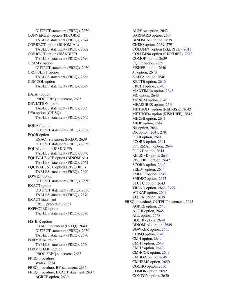
OUTPUT statement (FREQ), 2650CONVERGE= option (PLCORR)
TABLES statement (FREQ), 2674CORRECT option (BINOMIAL)
TABLES statement (FREQ), 2662CORRECT option (RISKDIFF)
TABLES statement (FREQ), 2690CRAMV option
OUTPUT statement (FREQ), 2650CROSSLIST option
TABLES statement (FREQ), 2668CUMCOL option
TABLES statement (FREQ), 2669
DATA= optionPROC FREQ statement, 2635
DEVIATION optionTABLES statement (FREQ), 2669
DF= option (CHISQ)TABLES statement (FREQ), 2665
EQKAP optionOUTPUT statement (FREQ), 2650
EQOR optionEXACT statement (FREQ), 2639OUTPUT statement (FREQ), 2650
EQUAL option (RISKDIFF)TABLES statement (FREQ), 2690
EQUIVALENCE option (BINOMIAL)TABLES statement (FREQ), 2662
EQUIVALENCE option (RISKDIFF)TABLES statement (FREQ), 2690
EQWKP optionOUTPUT statement (FREQ), 2650
EXACT optionOUTPUT statement (FREQ), 2650TABLES statement (FREQ), 2670
EXACT statementFREQ procedure, 2637
EXPECTED optionTABLES statement (FREQ), 2670
FISHER optionEXACT statement (FREQ), 2640OUTPUT statement (FREQ), 2650TABLES statement (FREQ), 2670
FORMAT= optionTABLES statement (FREQ), 2670
FORMCHAR= optionPROC FREQ statement, 2635
FREQ proceduresyntax, 2634
FREQ procedure, BY statement, 2636FREQ procedure, EXACT statement, 2637
AGREE option, 2639
ALPHA= option, 2643BARNARD option, 2639BINOMIAL option, 2639CHISQ option, 2639, 2791COLUMN= option (RELRISK), 2641COLUMN= option (RISKDIFF), 2642COMOR option, 2639EQOR option, 2639FISHER option, 2640JT option, 2640KAPPA option, 2640KENTB option, 2640LRCHI option, 2640MAXTIME= option, 2643MC option, 2643MCNEM option, 2640MEASURES option, 2640METHOD= option (RELRISK), 2642METHOD= option (RISKDIFF), 2642MHCHI option, 2641MIDP option, 2644N= option, 2644OR option, 2641, 2791PCHI option, 2641PCORR option, 2641PFORMAT= option, 2644POINT option, 2644RELRISK option, 2641RISKDIFF option, 2642SCORR option, 2642SEED= option, 2644SMDCR option, 2642SMDRC option, 2642STUTC option, 2643TREND option, 2643, 2799WTKAP option, 2643ZELEN option, 2639
FREQ procedure, OUTPUT statement, 2645AGREE option, 2648AJCHI option, 2648ALL option, 2648BDCHI option, 2648BINOMIAL option, 2649BOWKER option, 2655CHISQ option, 2649CMH option, 2649CMH1 option, 2649CMH2 option, 2649CMHCOR option, 2649CMHGA option, 2649CMHRMS option, 2650COCHQ option, 2650COMOR option, 2652CONTGY option, 2650

CRAMV option, 2650EQKAP option, 2650EQOR option, 2650EQWKP option, 2650EXACT option, 2650FISHER option, 2650GAILSIMON option, 2650GAMMA option, 2650JT option, 2651KAPPA option, 2651KENTB option, 2651LAMCR option, 2651LAMDAS option, 2651LAMRC option, 2651LGOR option, 2651LGRRC1 option, 2651LGRRC2 option, 2651LRCHI option, 2651MCNEM option, 2652MEASURES option, 2652MHCHI option, 2652MHOR option, 2652MHRRC1 option, 2652MHRRC2 option, 2652N option, 2652NMISS option, 2652OR option, 2652OUT= option, 2645output-options, 2645PCHI option, 2653PCORR option, 2653PLCORR option, 2653RDIF1 option, 2653RDIF2 option, 2653RELRISK option, 2653RISK1 option, 2654RISK11 option, 2654RISK12 option, 2654RISK2 option, 2654RISK21 option, 2654RISK22 option, 2655RISKDIFF option, 2653RISKDIFF1 option, 2653RISKDIFF2 option, 2654RRC1 option, 2654RRC2 option, 2654SCORR option, 2655SMDCR option, 2655SMDRC option, 2655STUTC option, 2655TAUB option, 2651TAUC option, 2655TREND option, 2655TSYMM option, 2655
U option, 2655UCR option, 2655URC option, 2655WTKAP option, 2656ZELEN option, 2650
FREQ procedure, PROC FREQ statement, 2634COMPRESS option, 2635DATA= option, 2635FORMCHAR= option, 2635NLEVELS option, 2636NOPRINT option, 2636ORDER= option, 2636PAGE option, 2636
FREQ procedure, TABLES statement, 2656AGREE option, 2659ALL option, 2660ALPHA= option, 2660BDT option (CMH), 2667BINOMIAL option, 2660CELLCHI2 option, 2664CHISQ option, 2664, 2791CL option, 2667CL= option (BINOMIAL), 2661CL= option (RISKDIFF), 2688CL=AGRESTICAFFO option (RISKDIFF), 2689CL=AGRESTICOULL option (BINOMIAL),
2661CL=ALL option (BINOMIAL), 2662CL=CLOPPERPEARSON option (BINOMIAL),
2662CL=EXACT option (BINOMIAL), 2662CL=EXACT option (RISKDIFF), 2689CL=HA option (RISKDIFF), 2689CL=JEFFREYS option (BINOMIAL), 2662CL=NEWCOMBE option (RISKDIFF), 2689CL=WALD option (BINOMIAL), 2662CL=WALD option (RISKDIFF), 2690CL=WILSON option (BINOMIAL), 2662CMH option, 2667CMH1 option, 2668CMH2 option, 2668COLUMN= option (RISKDIFF), 2690COMMON option (RISKDIFF), 2690CONTENTS= option, 2668CONVERGE= option (PLCORR), 2674CORRECT option (BINOMIAL), 2662CORRECT option (RISKDIFF), 2690CROSSLIST option, 2668CUMCOL option, 2669DEVIATION option, 2669DF= option (CHISQ), 2665EQUAL option (RISKDIFF), 2690EQUIVALENCE option (BINOMIAL), 2662EQUIVALENCE option (RISKDIFF), 2690

EXACT option, 2670EXPECTED option, 2670FISHER option, 2670FORMAT= option, 2670GAILSIMON option, 2670JT option, 2670LEVEL= option (BINOMIAL), 2663LIST option, 2671LRCHI option (CHISQ), 2665MANTELFLEISS option (CMH), 2667MARGIN= option (BINOMIAL), 2663MARGIN= option (RISKDIFF), 2690MAXITER= option (PLCORR), 2675MAXLEVELS= option, 2671MEASURES option, 2671METHOD= option (RISKDIFF), 2691METHOD=FM option (RISKDIFF), 2691METHOD=HA option (RISKDIFF), 2691METHOD=NEWCOMBE option (RISKDIFF),
2691METHOD=WALD option (RISKDIFF), 2691MISSING option, 2671MISSPRINT option, 2672NOCOL option, 2672NOCUM option, 2672NOFREQ option, 2672NONINFERIORITY option (BINOMIAL), 2663NONINFERIORITY option (RISKDIFF), 2691NOPERCENT option, 2672NOPRINT option, 2672NORISKS option (RISKDIFF), 2692NOROW option, 2672NOSPARSE option, 2672NOWARN option, 2673OR option, 2673, 2687OUT= option, 2674OUTCUM option, 2674OUTEXPECT option, 2674, 2779OUTPCT option, 2674P= option (BINOMIAL), 2664PEARSONRES option (CROSSLIST), 2669PLCORR option, 2674PLOTS= option, 2675PLOTS=AGREEPLOT option, 2676PLOTS=CUMFREQPLOT option, 2677PLOTS=DEVIATIONPLOT option, 2677PLOTS=FREQPLOT option, 2677PLOTS=KAPPAPLOT option, 2678PLOTS=MOSAICPLOT option, 2679PLOTS=NONE option, 2680PLOTS=ODDSRATIOPLOT option, 2680PLOTS=RELRISKPLOT option, 2680PLOTS=RISKDIFFPLOT option, 2681PLOTS=WTKAPPAPLOT, 2681
PRINTKWTS option, 2659, 2687RELRISK option, 2687, 2791RISKDIFF option, 2687SCORES= option, 2692, 2802SCOROUT option, 2692SPARSE option, 2693, 2779STDRES option (CROSSLIST), 2669SUPERIORITY option (BINOMIAL), 2664SUPERIORITY option (RISKDIFF), 2692TESTF= option, 2705TESTF= option (CHISQ), 2665TESTP= option, 2705, 2785TESTP= option (CHISQ), 2666TOTPCT option, 2693TREND option, 2693, 2799VAR= option (BINOMIAL), 2664VAR= option (RISKDIFF), 2692WARN= option (CHISQ), 2666
FREQ procedure, TEST statement, 2693AGREE option, 2694GAMMA option, 2694KAPPA option, 2695KENTB option, 2695MEASURES option, 2695PCORR option, 2695PLCORR option, 2695SCORR option, 2695SMDCR option, 2696, 2799SMDRC option, 2696STUTC option, 2696TAUB option, 2695TAUC option, 2696WTKAP option, 2696
FREQ procedure, WEIGHT statement, 2696ZEROS option, 2697
GAILSIMON optionOUTPUT statement (FREQ), 2650TABLES statement (FREQ), 2670
GAMMA optionOUTPUT statement (FREQ), 2650TEST statement (FREQ), 2694
JT optionEXACT statement (FREQ), 2640OUTPUT statement (FREQ), 2651TABLES statement (FREQ), 2670
KAPPA optionEXACT statement (FREQ), 2640OUTPUT statement (FREQ), 2651TEST statement (FREQ), 2695
KENTB optionEXACT statement (FREQ), 2640OUTPUT statement (FREQ), 2651

TEST statement (FREQ), 2695
LAMCR optionOUTPUT statement (FREQ), 2651
LAMDAS optionOUTPUT statement (FREQ), 2651
LAMRC optionOUTPUT statement (FREQ), 2651
LEVEL= option (BINOMIAL)TABLES statement (FREQ), 2663
LGOR optionOUTPUT statement (FREQ), 2651
LGRRC1 optionOUTPUT statement (FREQ), 2651
LGRRC2 optionOUTPUT statement (FREQ), 2651
LIST optionTABLES statement (FREQ), 2671
LRCHI optionEXACT statement (FREQ), 2640OUTPUT statement (FREQ), 2651
LRCHI option (CHISQ)TABLES statement (FREQ), 2665
MANTELFLEISS option (CMH)TABLES statement (FREQ), 2667
MARGIN= option (BINOMIAL)TABLES statement (FREQ), 2663
MARGIN= option (RISKDIFF)TABLES statement (FREQ), 2690
MAXITER= option (PLCORR)TABLES statement (FREQ), 2675
MAXLEVELS= optionTABLES statement (FREQ), 2671
MAXTIME= optionEXACT statement (FREQ), 2643
MC optionEXACT statement (FREQ), 2643
MCNEM optionEXACT statement (FREQ), 2640OUTPUT statement (FREQ), 2652
MEASURES optionEXACT statement (FREQ), 2640OUTPUT statement (FREQ), 2652TABLES statement (FREQ), 2671TEST statement (FREQ), 2695
METHOD= option (RELRISK)EXACT statement (FREQ), 2642
METHOD= option (RISKDIFF)EXACT statement (FREQ), 2642TABLES statement (FREQ), 2691
METHOD=FM option (RISKDIFF)TABLES statement (FREQ), 2691
METHOD=HA option (RISKDIFF)
TABLES statement (FREQ), 2691METHOD=NEWCOMBE option (RISKDIFF)
TABLES statement (FREQ), 2691METHOD=WALD option (RISKDIFF)
TABLES statement (FREQ), 2691MHCHI option
EXACT statement (FREQ), 2641OUTPUT statement (FREQ), 2652
MHOR optionOUTPUT statement (FREQ), 2652
MHRRC1 optionOUTPUT statement (FREQ), 2652
MHRRC2 optionOUTPUT statement (FREQ), 2652
MIDP optionEXACT statement (NPAR1WAY), 2644
MISSING optionTABLES statement (FREQ), 2671
MISSPRINT optionTABLES statement (FREQ), 2672
N optionOUTPUT statement (FREQ), 2652
N= optionEXACT statement (FREQ), 2644
NLEVELS optionPROC FREQ statement, 2636
NMISS optionOUTPUT statement (FREQ), 2652
NOCOL optionTABLES statement (FREQ), 2672
NOCUM optionTABLES statement (FREQ), 2672
NOFREQ optionTABLES statement (FREQ), 2672
NONINFERIORITY option (BINOMIAL)TABLES statement (FREQ), 2663
NONINFERIORITY option (RISKDIFF)TABLES statement (FREQ), 2691
NOPERCENT optionTABLES statement (FREQ), 2672
NOPRINT optionPROC FREQ statement, 2636TABLES statement (FREQ), 2672
NORISKS option (RISKDIFF)TABLES statement (FREQ), 2692
NOROW optionTABLES statement (FREQ), 2672
NOSPARSE optionTABLES statement (FREQ), 2672
NOWARN optionTABLES statement (FREQ), 2673
OR option

EXACT statement (FREQ), 2641, 2791OUTPUT statement (FREQ), 2652TABLES statement (FREQ), 2673, 2687
ORDER= optionPROC FREQ statement, 2636
OUT= optionOUTPUT statement (FREQ), 2645TABLES statement (FREQ), 2674
OUTCUM optionTABLES statement (FREQ), 2674
OUTEXPECT optionTABLES statement (FREQ), 2674, 2779
OUTPCT optionTABLES statement (FREQ), 2674
OUTPUT statementFREQ procedure, 2645
P= option (BINOMIAL)TABLES statement (FREQ), 2664
PAGE optionPROC FREQ statement, 2636
PCHI optionEXACT statement (FREQ), 2641OUTPUT statement (FREQ), 2653
PCORR optionEXACT statement (FREQ), 2641OUTPUT statement (FREQ), 2653TEST statement (FREQ), 2695
PEARSONRES option (CROSSLIST)TABLES statement (FREQ), 2669
PFORMAT= optionEXACT statement (FREQ), 2644
PLCORR optionOUTPUT statement (FREQ), 2653TABLES statement (FREQ), 2674TEST statement (FREQ), 2695
PLOTS= optionTABLES statement (FREQ), 2675
PLOTS=AGREEPLOT optionTABLES statement (FREQ), 2676
PLOTS=CUMFREQPLOT optionTABLES statement (FREQ), 2677
PLOTS=DEVIATIONPLOT optionTABLES statement (FREQ), 2677
PLOTS=FREQPLOT optionTABLES statement (FREQ), 2677
PLOTS=KAPPAPLOT optionTABLES statement (FREQ), 2678
PLOTS=MOSAICPLOT optionTABLES statement (FREQ), 2679
PLOTS=NONE optionTABLES statement (FREQ), 2680
PLOTS=ODDSRATIOPLOT optionTABLES statement (FREQ), 2680
PLOTS=RELRISKPLOT optionTABLES statement (FREQ), 2680
PLOTS=RISKDIFFPLOT optionTABLES statement (FREQ), 2681
PLOTS=WTKAPPAPLOT optionTABLES statement (FREQ), 2681
POINT optionEXACT statement (FREQ), 2644
PRINTKWTS optionTABLES statement (FREQ), 2659, 2687
PROC FREQ statement, see FREQ procedure
RDIF1 optionOUTPUT statement (FREQ), 2653
RDIF2 optionOUTPUT statement (FREQ), 2653
RELRISK optionEXACT statement (FREQ), 2641OUTPUT statement (FREQ), 2653TABLES statement (FREQ), 2687, 2791
RISK1 optionOUTPUT statement (FREQ), 2654
RISK11 optionOUTPUT statement (FREQ), 2654
RISK12 optionOUTPUT statement (FREQ), 2654
RISK2 optionOUTPUT statement (FREQ), 2654
RISK21 optionOUTPUT statement (FREQ), 2654
RISK22 optionOUTPUT statement (FREQ), 2655
RISKDIFF optionEXACT statement (FREQ), 2642OUTPUT statement (FREQ), 2653TABLES statement (FREQ), 2687
RISKDIFF1 optionOUTPUT statement (FREQ), 2653
RISKDIFF2 optionOUTPUT statement (FREQ), 2654
RRC1 optionOUTPUT statement (FREQ), 2654
RRC2 optionOUTPUT statement (FREQ), 2654
SCORES= optionTABLES statement (FREQ), 2692, 2802
SCOROUT optionTABLES statement (FREQ), 2692
SCORR optionEXACT statement (FREQ), 2642OUTPUT statement (FREQ), 2655TEST statement (FREQ), 2695
SEED= option
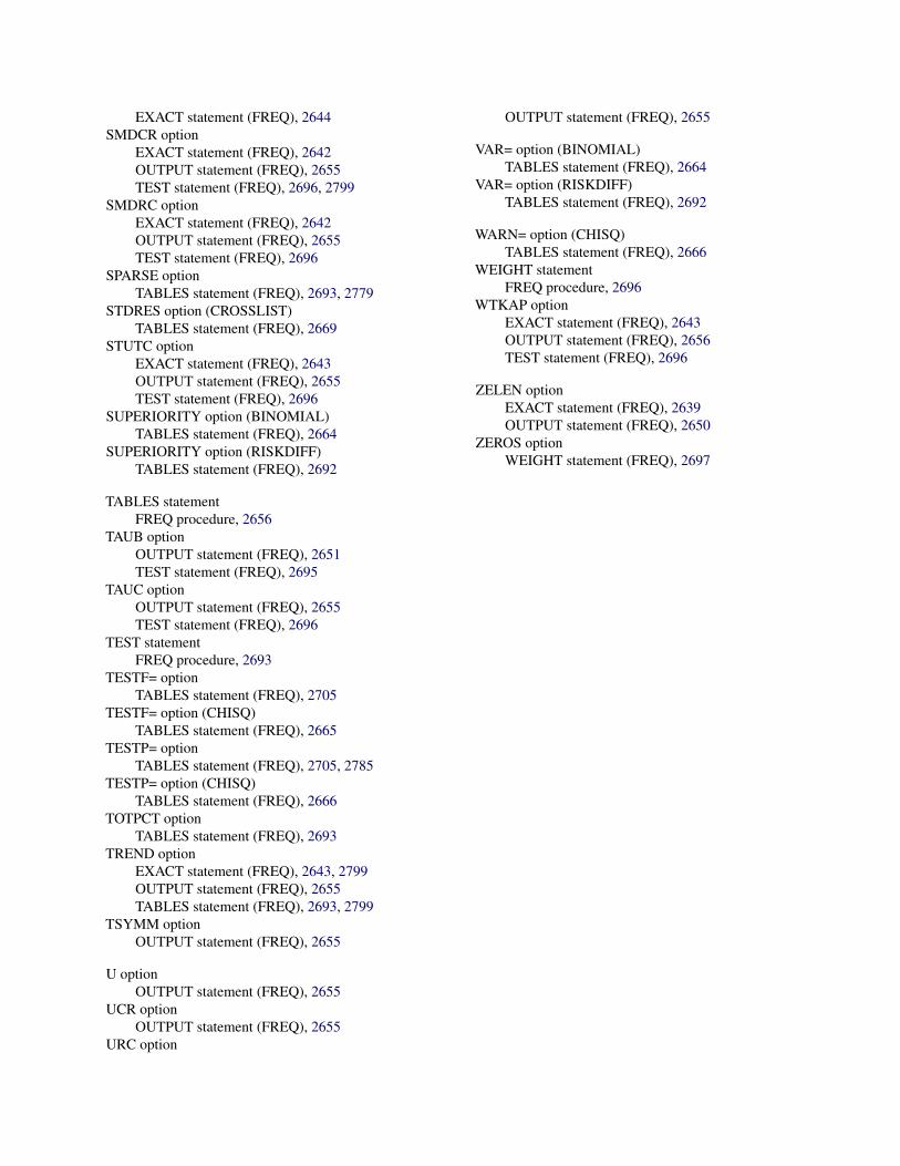
EXACT statement (FREQ), 2644SMDCR option
EXACT statement (FREQ), 2642OUTPUT statement (FREQ), 2655TEST statement (FREQ), 2696, 2799
SMDRC optionEXACT statement (FREQ), 2642OUTPUT statement (FREQ), 2655TEST statement (FREQ), 2696
SPARSE optionTABLES statement (FREQ), 2693, 2779
STDRES option (CROSSLIST)TABLES statement (FREQ), 2669
STUTC optionEXACT statement (FREQ), 2643OUTPUT statement (FREQ), 2655TEST statement (FREQ), 2696
SUPERIORITY option (BINOMIAL)TABLES statement (FREQ), 2664
SUPERIORITY option (RISKDIFF)TABLES statement (FREQ), 2692
TABLES statementFREQ procedure, 2656
TAUB optionOUTPUT statement (FREQ), 2651TEST statement (FREQ), 2695
TAUC optionOUTPUT statement (FREQ), 2655TEST statement (FREQ), 2696
TEST statementFREQ procedure, 2693
TESTF= optionTABLES statement (FREQ), 2705
TESTF= option (CHISQ)TABLES statement (FREQ), 2665
TESTP= optionTABLES statement (FREQ), 2705, 2785
TESTP= option (CHISQ)TABLES statement (FREQ), 2666
TOTPCT optionTABLES statement (FREQ), 2693
TREND optionEXACT statement (FREQ), 2643, 2799OUTPUT statement (FREQ), 2655TABLES statement (FREQ), 2693, 2799
TSYMM optionOUTPUT statement (FREQ), 2655
U optionOUTPUT statement (FREQ), 2655
UCR optionOUTPUT statement (FREQ), 2655
URC option
OUTPUT statement (FREQ), 2655
VAR= option (BINOMIAL)TABLES statement (FREQ), 2664
VAR= option (RISKDIFF)TABLES statement (FREQ), 2692
WARN= option (CHISQ)TABLES statement (FREQ), 2666
WEIGHT statementFREQ procedure, 2696
WTKAP optionEXACT statement (FREQ), 2643OUTPUT statement (FREQ), 2656TEST statement (FREQ), 2696
ZELEN optionEXACT statement (FREQ), 2639OUTPUT statement (FREQ), 2650
ZEROS optionWEIGHT statement (FREQ), 2697