The free electron -...

EE 439 free electrons & scattering –

The free electron

In order to develop our practical understanding with quantum mechanics, we’ll start with some simpler one-dimensional (function of x only), time-independent problems. At one time, such problems were considered “textbook” only situations. But in the last 25 years or so, 1-D wells and barriers nearly identical to the ones we will discuss have been built using semiconductor heterojunction technologies. Quantum wells are used in common devices like QW FETs (used in cell phones and satellite communication systems) and QW lasers (used in DVD players). Also, the gate oxide layers in flash memory are tunneling barriers, designed to allow electrons to leak through under the right circumstances.

Although we could use other types of particles in our examples, we will generally use electrons, since they are key in the behavior of nanoelectronic devices.

1


We’ve already solved this problem. The free electron moves in a potential-free region, U = 0. In that case, the time-independentSchroedinger equation is

�~2

2m

@

2 (x)

@x

2= E (x)

This can be re-written as

@

2 (x)

@x

2+

2mE

~2 (x) = 0

@

2 (x)

@x

2+ k

2 (x) = 0 k =

r2mE

~2

(x) = A exp(ikx) + B exp(�ikx)

The general solution is:

This represents plane waves traveling in the +x (first term) and -x directions. (Don’t forget about the implicit time dependence.)

2


k =

r2mE

~2 (x) = A exp(ikx) + B exp(�ikx)

There should be no surprise here. We justified the S.E. by looking for this particular solution.

Note that we must include the possibility of travel in either direction. In looking at more specific problems, boundary conditions (or the way that we set up a problem) may let us choose to leave off one term or the other.

The electron energy can take on any value > 0 — there is no quantization.

� =E

h� =

h

k=

hp2mE

3


The parabolic E-k (E-p) is indicative of a free electron. This is identical to the classical result.

E =(~k)2

2m

Ener

gy (E

)wave number (k)

(or momentum, p)

4


If we try to complete the problem and normalize the wave function, things get a bit odd, as we had discussed earlier. To see the source of the difficulty more clearly, consider an electron known to be moving in the +x direction, so that we can leave off the second term in the general solution.

+

(x) = A exp(ikx)

Z +1

�1

⇤(x) (x)dx = 1

The normalization condition is

Z+1

�1[A

⇤exp (�ikx)] [A exp (+ikx)] dx = 1

Z +1

�1|A|2 dx = 1

First note that the probability density is a simple constant — there is equal probability that the electron can be at any value of x. This is in line with our notions of a plane wave and the uncertainty principle.

5


But here’s the bad news: the only way that the normalization can be met is if |A|2 → 0. In other words, the amplitude of the wave must be vanishingly small at all points.

In effect, we are saying the electron must be simultaneously everywhere and nowhere. Of course, this is absurd. And it really isn’t a good description of the free electron. Yes, the wave function is a valid solution of the S.E., but it fails the basic test of describing a particle that is in some sense localized in space.

In order to fix this conundrum, we’ll have to use the superposition principle to add together a collection of valid solutions to create what we call a wave packet. This will also lead us to a consideration of the uncertainty principle. However, we’ll save this to later.

6


Electrons incident on an energy stepNow consider an electron incident on a step in the energy. The step goes from a constant region where U = 0 to one with a different constant value of potential energy Uo. The energy of the incident electron is E > Uo.

U = Uo

U = 0

x = 0

E > Uo

1 2

Classically, we would assume that the electron zooms over the step, completely unaware of its presence. When the electron is described by a wave however, things are not that simple.

7


The approach to this kind of problem is to break it into pieces. For instance, we already know the solution in the region where U = 0. (It’s a free electron!) And we can probably find the solution for the other region without much trouble. Then we can “connect” to the solutions at the interface. So we need to determine the connection rules for step interfaces in 1-D problems.

The place to start is with the requirement that the wave function and the derivative of the wave function must be both be continuous. We might assume that these conditions must remain true at the interface (as long as the interface isn’t too weird), but it’s not necessarily obvious that this should be the case.

�(0) = +(0) 0�(0) = 0

+(0)

8


We can strengthen the argument by looking at the step interface as the limit of a gradual change in potential from one level to another.

00(x) =2m

~2[U(x) � E] (x)

Integrating once from point a to some arbitrary point x

0(x) =

0(a) +2m

~2

Zx

a

[U(y) � E] (y)dy

x = a x = bU(a)

U(b)

Start by writing the Schroedinger equation, in a slightly modified form:

9


Integrating a second time from x = a to x = b

(b) = (a) +

0(a) · (b � a) +2m

~2

Zb

a

Zx

a

[U(y) � E] (y)dydx

Now, let the gradual change sharpen up to an abrupt change from one level to the other. This means looking at the limit as b→a. In this case, the previous two equations reduce to

0(b) = 0(a) (b) = (a)

As we expected.

In particular, letting x=b

0(b) = 0(a) +2m

~2

Z b

a[U(y) � E] (y)dy

10


Now, back to our step problem. Again, we will find solutions in the two regions of constant potential and then connect them at the interface using our newly found connection rules.

In the region x > 0, where U = Uo, the Schroedinger equation is

�~2

2m

@

2 (x)

@x

2+ U

o

(x) = E (x)

@

2 (x)

@x

2+

2m

~2(E � U

o

) (x) = 0

In the region 1, x < 0, where U = 0, we already know the solutions.

1

(x) = A exp(ik

1

x) + B exp(�ik

1

x)

k1 =

r2mE

~2

11


@

2 (x)

@x

2+

2m

~2(E � U

o

) (x) = 0

Note that this has general form of the free electron problem, except that the energy factor in the second term is E – Uo instead of just E, as in the free electron case. So in region 2, the solutions should also have the form of plane waves, but with a different value of k.

k2 =

s2m(E � U

o

)

~2

2

(x) = C exp(ik

2

x) + D exp(�ik

2

x)

Before going further, we should decide what we are looking for. In this case, we might be interested in looking at the probability of the electron being reflected or transmitted at the step. Conceptually, the “experiment” might go something like this: Send an electron from the left in region 1 towards the step (This is represented by amplitude A.), and look for what is reflected back into region 1 (amplitude B) and transmitted into the other region (amplitude C). This is known as a “scattering” problem.

12


In this situation, the amplitude D, representing a wave coming from the right in region 2, has no role. In fact, including it would complicate the relatively simple picture. So we choose to leave it out.

2

(x) = C exp(ik

2

x)

Also, we are primarily interested in the ratios B/A and C/A, which would represent reflection and transmission amplitudes, respectively. The problem has now been reduced to something manageable.

All that is left is to use the connection rules at x = 0 to match the solutions from the two regions.

13


1(0) = 2(0)

A + B = C

01(0) = 0

2(0)

ik1A � ik1B = ik2C

This gives two equations that can be solved for the two ratios B/A and C/A. Grunting through the algebra gives (Be sure to do this for yourself.):

B/A =k1 � k2

k1 + k2

C/A =2k1

k1 + k2

A remarkable result is immediately apparent: Since B/A ≠ 0, the electron may be reflected from the step, even though E > Uo.

14

EE 439 free electrons & scattering – 15

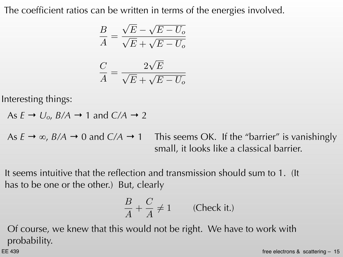
The coefficient ratios can be written in terms of the energies involved.

B

A=

pE �

pE � U

opE +

pE � U

o

C

A=

2pEp

E +pE � U

o

Interesting things:

As E → Uo, B/A → 1 and C/A → 2

As E → ∞, B/A → 0 and C/A → 1 This seems OK. If the “barrier” is vanishingly small, it looks like a classical barrier.

It seems intuitive that the reflection and transmission should sum to 1. (It has to be one or the other.) But, clearly

B

A+

C

A6= 1 (Check it.)

Of course, we knew that this would not be right. We have to work with probability.


✓B

A

◆⇤ ✓B

A

◆= |B

A|2 =

(k1 � k2)2

(k1 + k2)2

✓C

A

◆⇤ ✓C

A

◆= |C

A|2= 4k21

(k1 + k2)2

Using probability densities:

Oops. Those don’t add up to 1 either. What’s going on here?


Probability flux

Probability densities are stationery — as they must be for a solution to the TISE. They give information about the likelihood of finding the electron at a particular place. We are looking for the likelihood of reflection or transmission for an electron propagating towards a step. Somehow, we must incorporate the notion that the the electron is moving and scattering from the step.

We need the “probability flux”. To get there, we start with the idea that an indestructible object, like an electron, must maintain normalization, i.e. once the wave function is normalized, it must remain normalized. Mathematically,

d

dt

Z 1

�1| |2dx = 0

Any wave function that is a solution to the Schroedinger equation will satisfy this condition.


@| |2

@t

=i~2m

" ⇤@

2

@x

2�

@

2 ⇤

@x

2

#

Substituting in and noting that some terms cancel:

@

@t

=i~2m

@

2

@x

2� i

~U

We can use the Schroedinger equation to find an expression for the time-derivative of the wave function, and its complex conjugate

@ ⇤

@t

=�i~2m

@

2 ⇤

@x

2+

i

~U

For the time-derivative of the probability density

@| |2

@t=

@ ( ⇤)

@t= ⇤ @

@t+

@ ⇤

@t


This can be re-written slightly

@| |2

@t

=@

@x

i~2m

✓ ⇤@

@x

� @ ⇤

@x

◆�

19

Look carefully at what this equations is saying to us. The time-derivative of a density function (in this case, probability density) is equal to the spatial derivative of something else. You’ve seen these kind of equation before — it is a continuity relation. The quantity inside the bracket must be a flux (or current).

@⇢

@t

=@j

@x

@N

@t

=@F

@x

Diffusion of dopant atoms in a crystal (EE 432)

charge in a semiconductor (EE 432)


The quantity in brackets is the probability flux.

Recall that flux is a quantity per unit area per unit time. Flux is a way of defining the flow of a quantity. Fluxes are the quantities that should be conserved in the scattering situation: incident flux = reflected flux + transmitted flux.

Fp = � i~2m

✓ ⇤ @

@x

� @ ⇤

@x

◆

The probability flux for a free electron traveling in the +x-direction: + (x) = Ae

ikx

F+ =~km

|A|2

F+ = � i~2m

⇥�A⇤e�ikx

� �ikAe+ikx

��Ae+ikx

� ��ikA⇤e�ikx

�⇤


Applying these results to the scattering problem

The reflection coefficient would be the ratio of the reflected probability flux to the incoming probability flux. (Be careful with the negative sign on the negative-traveling flux) The transmission coefficient is the ratio of the transmitted flux to the incident flux.

21

F1+ =~k1m

|A|2 F1� = �~k1m

|B|2 F2+ =~k2m

|C|2

incident flux reflected flux transmitted flux

note the neg. sign

R =|F1�|F1+

=~k1m |B|2~k1m |A|2

=|B|2

|A|2 T =F2+

F1+=

~k2m |C|2~k1m |A|2

=k2|C|2

k1|A|2

Note that R + T = 1, which is a comforting result. The coefficients can also be expressed in terms of the relevant energies. (Try it.)

The free electron -...

Documents

Transcript of The free electron -...