The Fractal Pattern of the French Gothic Cathedrals … · 2017-08-24 · The Fractal Pattern of...

RESEARCH

The Fractal Pattern of the French Gothic Cathedrals

Albert Samper • Blas Herrera

Published online: 9 May 2014

� Kim Williams Books, Turin 2014

Abstract The classic patterns of Euclidean Geometry were used in the con-

struction of the Gothic cathedrals to provide them with proportion and beauty. Still,

there is also another complex concept related to them: the un-evenness of their

structures, which determines their space-filling ability, that is, their level of

roughness. In this paper we use the techniques of Fractal Geometry to generate

parameters which provide a measure of roughness. In this way we show that the

French Gothic cathedrals do not only follow Euclidean geometric patterns, but also

have a general non-random fractal pattern.

Keywords French Gothic � Fractal parameter � Fractal dimension �Gothic architecture

Introduction

Benoit Mandelbrot was the main developer of Fractal Geometry in the late 1970s.

His theories have evolved and have been used in several fields including

architecture. Inspired by Mandelbrot’s work, Bechhoefer and Bovill used the

concept of fractal dimension in architectural drawings (Bechhoefer and Bovill 1994;

Bovill 1996). As a result of this work, many authors (see Ostwald et al. 2008;

Vaughan and Ostwald 2009, 2010, 2011; Ostwald and Vaughan 2009, 2010) used

similar techniques to analyze the design of certain architects such as Le Corbusier,

A. Samper

Unitat predepartamental d’Arquitectura, Universitat Rovira i Virgili,

Avinguda Paısos Catalans 26, 43007 Tarragona, Spain

B. Herrera (&)

Departament d’Enginyeria Informatica i Matematiques, Universitat Rovira i Virgili,

Avinguda Paısos Catalans 26, 43007 Tarragona, Spain

e-mail: [email protected]

Nexus Netw J (2014) 16:251–271

DOI 10.1007/s00004-014-0187-7

Frank Lloyd Wright, Peter Eisenman and Eileen Gray. Specifically, those authors

looked for a relation between the structure of the architects’ constructions and the

natural or artificial environment where those constructions were projected. These

techniques have also been used in other kinds of architectural studies (see Bovill

1996; Eglash 1999; Batty and Longley 2001; Burkle-Elizondo 2001; Ostwald 2001,

2010; Crompton 2002; Brown and Witschey 2003; Cooper 2003; Sala 2006;

Hammer 2006; Joye 2007; Rian et al. 2007; Bovill 2008; Ostwald and Vaughan

2013). These works are based on a geometrical concept which is called fractal

dimension. In this paper we will use this concept in order to generate what we will

call fractal parameter; and by means of this parameter we will study the existence

of a yet unknown pattern in French Gothic cathedrals. This generated fractal

parameter will give a measure of the unevenness of their structures, which in turn

determines their space-filling ability, which is also a measure of their level of

roughness.

Historical Setting

Gothic cathedrals are widely accepted as being among the most important art

creations of mankind. They are the result of religious interests, aesthetic patterns

and social influences, and their making brought together great scientific know-how

(Wilson 1990; Baldellou 1995; Toman 1998; Prache 2000; Schutz 2008). The style

of architecture we now call Gothic first emerged between the 12th and 15th

centuries of the medieval period. It emphasized structural lightness and illumination

of the inside naves. It arises in contrast to the massiveness and the inadequate

interior illumination of Romanic churches. It evolved mainly within ecclesiastical

architecture, especially cathedrals.

Gothic art was born in northern France, in a region called ‘‘Ile de France’’ to be

precise. Historically, this style was marked by the alliance between the French

monarchy and the Catholic Church. The first trial of Gothic architecture took place

in Saint Denis under the patronage of abbot Suger, friend and confident of Louis VI.

Following the example of Saint Denis, several primeval Gothic buildings were built

in the second half of the 12th century. In Laon cathedral (1156–1160) and Notre

Dame cathedral (1163), the central nave was raised and the light became the

dominant element. It was also then that construction of Chartres cathedral began.

There, the architect abandoned entirely the use of the tribune gallery and introduced

the use of simple ribbed vaults. From the 13th century onward, after these first trials,

the Gothic style entered its classical stage. The best examples are the Reims

cathedral (1211) and the Amiens cathedral (1220). Both have a cross-shaped floor

plan and their elements were combined in pursuit of illumination and structural

lightness and regularity. The classical Gothic style was adapted in France into

numerous regional ramifications.

Significant Sample and Geometrical Patterns

Our study focuses into a subset of 20 French cathedrals which are predominantly

Gothic in style, were built in the region called Ile de France between the 11th and

252 A. Samper, B. Herrera

13th centuries, and are representative of the total population of Gothic cathedrals

(Fig. 1).

This sample of cathedrals is considered to be significant in stylistic, chronolog-

ical and geographical terms. We intend to analyse the constructions geometrically

using new parameters which were unknown until now. Since each construction had

its very own authorship and circumstances, we have not gone on to compare

cathedrals with each other. Instead, we have examined if the design traits and

structures of these constructions have a deeper geometrical sense than is known to

us yet.

Fig. 1 Geographical situation of the 20 cathedrals being studied: Strasbourg cathedral (1015), Troyescathedral (1128), Sens cathedral (1135), Noyon cathedral (1150), Senlis cathedral (1153), Laon cathedral(1155), Paris cathedral (1163), Lisieux cathedral (1170), Tours cathedral (1170), Soissons cathedral(1177), Chartres cathedral (1195), Bourges cathedral (1195), Rouen cathedral (1202), Reims cathedral(1211), Auxerre cathedral (1215), Amiens cathedral (1220), Metz cathedral (1220), Orleans cathedral(1278), Toul cathedral (13th century), Sees cathedral (13th–14th century)

The Fractal Pattern of the French Gothic Cathedrals 253

The master craftsman had to be extensively knowledgeable about mathematics,

particularly about geometry, as we can see from the sketchbooks of architect Villard

de Honnecourt (Bechmann 1985). We must bear in mind that they didn’t have a

precise scale to measure fractions smaller than a toise or a foot-length and transport

them accurately to bigger units. Therefore, it was safer to take a geometric outline as

the starting point for the construction; for instance a square mesh like the ones used

for the Roman and pre-Gothic basilicas and for the Roman fortified camps. As well

as the square, architects used the pentagon, the octagon and the decagon (all of them

constructible using a ruler and a compass) to represent, by means of accurate

geometric relations, the floor plans and elevations of their constructions (Simon

1985). The square, as well as the octagon, stemmed from geometries which took the

heavenly Jerusalem as a model. Nonetheless, the most perfect proportion stems

from the pentagon and the decagon, leading to the golden ratio phi (Fig. 2).

The classic patterns of the Euclidean Geometry, such as coefficients phi and pi,

were used in Gothic constructions to provide them with proportion and beauty

(Fig. 3). As well as the Euclidean elements, however, there is another complex

concept in the construction of the Gothic cathedrals: the unevenness of their

structures, which determines their space-filling ability, i.e. their level of roughness.

The best tool to describe this concept is given by Fractal Geometry through a ratio

called fractal dimension. We will generate a geometrical parameter, called fractal

Fig. 2 Amiens Cathedral, geometric development of the Floor plan


parameter, which will give a measure of roughness. As well as being attributable to

Euclidean elements, this fractal parameter is generated by the final architectonic

result of the constructions.

The aim of our investigation is to analyse the geometry of the French Gothic

cathedrals in order to show the existence of a general fractal pattern. We are not

comparing the constructive processes of the cathedrals nor the will of the architects

to implement their designs. Instead, we will demonstrate that the geometry of their

compositions shows a common formal pattern.

Fractal Parameter and Method

The first step of our investigation was to collect as many graphic documents as

possible from all the cathedrals being studied. The main information sources were:

the respective archdioceses of the cathedrals (we thank them for providing us with

specially clear and precise graphic papers); Jean-Charles Forgeret, in charge of the

Mediatheque de l’Architecture et du Patrimoine, who provided us with original

historical drawings for the different parts of each cathedral; Martine Mauvieux, in

charge of the Departement des Estampes et de la Photographie de la Bibliotheque

Nationale de France, who offered a large number of photographs and drawings

which we used for redrawing; the Archivo del Colegio de Arquitectos de Catalunya;

and the Biblioteca de la Escuela Tecnica Superior de Arquitectura de Barcelona,

where we found some very illustrative monographs (see Murray 1996; Kunst and

Schekluhn 1996) which let us complete the study.

All documents collected have been redrawn by us with CAD tools in order to

attain the highest level of objectivity, homogeneous graphic display criteria and the

same level of detail, without taking textures into account (Ostwald and Vaughan

2013), using black color and line width *0.00 mm (that is, the minimal lineweight

allowed using CAD software), see Fig. 4. This was absolutely necessary, since the

information collected had different styles and, in general, a very low, inadequate

resolution to be able to apply the calculations.

So, in order to establish the fractal parameter of the French Gothic architecture,

we leave ornaments aside and we take three basic projections of the cathedral’s

structure: floor plan, main elevation and cross-section. Working on these

projections, we make the corresponding mathematical calculations. Figure 4 shows

the detail level of the redrawing. Figures 7, 8 and 9 show the redrawing made for

Fig. 3 Amiens Cathedral, geometric outline. Module A is 40 feet; module B is 110 feet


these basic projections of the 20 cathedrals being studied (redrawing is in a small

scale to keep the paper reasonably short).

We have strictly followed precise drawing lines, highlighting the lines which best

represent the geometry of the floor plan, main elevation and cross-section. As we

have stated before, this redrawing is absolutely necessary, since the documents

collected consist of drawings or photographs with shadows, stains, colors, defects,

freehand lines, etc.; i.e. all graphic documents show ‘‘noise’’, so we had to do again

each and every one of the drawings which appear in this paper.

Summary of the Fractal Parameter’s Generation Process

Architectural structures, from now on called M, are not fractal objects. Despite that,

we can consider M’s unevenness and its space-filling ability, that is, its level of

roughness. Also, we can generate a parameter for these non-fractal objects, the

fractal parameter Ps(M). The value provided by this fractal parameter Ps(M) is a

measure of the level of roughness of the architectural structure being studied M.

The process to generate Ps(M) through calculations with a self-created software

is summarized as follows:

1. Given the architectural structure M, first we generate its design in AutoCad

vector format, using black color and line width *0.00 mm. From this AutoCad

format we obtain the pdf vector format.

2. From the pdf vector format we generate a black-and-white digital bitmap file,

sized 1,024 9 t pixels, showing the architectural structure with its size adjusted

to full width and height.

3. Ps(M)—using a self-created software, we calculate the fractal parameter

Ps(M) based on the slope on the last point of a continuous graph ln–ln. In the

following sections we explain which continuous graph we are talking about and

which calculations are made.

The value Ps(M) is a fractal parameter of the structure M, which gives a measure

of its level of roughness.

Fig. 4 Detail level of the redrawings: on the left, a detail of Chartres cathedral’s ambulatory. In themiddle, a detail of Reims cathedral’s main elevation. On the right, a detail of a module of the centralnave’s cross-section in Amiens Cathedral


The reason to create for ourselves a special software is twofold: firstly, we will

have total control of the calculations and so we will ensure these calculations are

correct. Secondly, commercial software like Benoit does not use the slope on the

last point of the continuous graph ln–ln. Benoit uses the slope of the regression line

corresponding to the discrete set of points in the graph ln–ln.

However, the slope of the regression line is only similar to the fractal dimension

when M is a fractal self-similar object, because then its continuous graph ln–ln is a

straight line. But an architectural structure M is not a fractal object nor a self-similar

fractal object, so its continuous graph ln–ln is not a straight line (later on we will

define a fractal object and a fractal self-similar object). M does not possess fractal

geometry but it does have a fractal parameter Ps(M); we will generate this parameter

Ps(M) with a process which has been extrapolated from the theoretical limit �FðMÞ,called upper fractal dimension of M, M being a non self-similar fractal object (this

process will be explained later).

In any case, if we change step 3 above and instead we use the calculation for the

slope of the regression line corresponding to the discrete set of points, then we

obtain another fractal parameter which we will call Pr(M). For this calculation we

can use either our self-created software or Benoit. Then step 3 is as follows:

3. Pr(M)—using either a self-created software or the commercial software Benoit,

we calculate the fractal parameter Pr(M) based on the slope of the regression line

corresponding to the discrete set of points in the graph ln–ln; and for this

calculation we use square meshes, the finest mesh having 4 9 4 pixel squares,

and the coarsest mesh having 32 9 32 pixel squares.

The reason for using square meshes with these particular limits of fineness and

coarseness will be explained later.

We may also consider another variation of the fractal parameter if we change step

3 of the process above and instead we make the calculations with the variables

which the commercial software Benoit uses by default. The new parameter thus

obtained is called Pb(M). Then step 3 is as follows:

3. Pb(M)—using the commercial software Benoit we calculate the fractal

parameter Pb(M) based on the regression line corresponding to the discrete set of

points in the graph ln–ln, and for this calculation we use square meshes, the finest

mesh having 1 9 1 pixel squares and the coarsest mesh having 256 9 256 pixel

squares.

To sum up, we have created software to obtain the value Ps(M) because the

structures M being considered are not self-similar objects, but we also calculate the

values Pr(M) and Pb(M). These three measures are not equal because the calculation

methods are different. However, all three give a measure of the roughness of the

structure.

In this paper we calculate and use the three parameters Ps(M), Pr(M) and

Pb(M) in order to show, beyond any doubt, the existence of a fractal pattern in

Gothic structures. At the end of this paper we will see the results and relationships

between the three measures.


Hausdorff–Besicovitch Dimension

Readers may skip this very technical subsection and still fully understand the work

which is presented in this paper. We provide book references to interest readers. In

this section we summarize the dimensions TðMÞ;HðMÞ; �FðMÞ;FðMÞ;HðMÞ; SðMÞof the fractal objects M; and some of their properties. This is the theoretical basis

from which the ideas for generating the fractal parameter Ps(M) arise.

Let M be a bounded non-empty subset of the n-dimensional Euclidean affine

space, An. The definition of the s-dimensional Hausdorff measure of M, HsðMÞ, can

be found in (Falconer 1990, 1997; Edgar 1998) or in other books about fractals.

There is also a theorem which states as follows: there is a critical value HðMÞ such

that: HsðMÞ ¼ 1 if 0 B s \HðMÞ, and HsðMÞ ¼ 0 if s [HðMÞ. If s = HðMÞ,then HsðMÞ 2 ½0;1�. This critical value HðMÞ is called Hausdoff-Besicovitch

dimension of M. Moreover, M has its topological dimension, T (M). We have the

following geometric definition: M is a fractal object if HðMÞ[ T (M).

The Hausdorff–Besicovitch dimension has an upper bound �FðMÞ[ HðMÞ. This

upper bound �FðMÞ is called Minkowski-Bouligand dimension of M � An, and we

will call it upper fractal dimension of M. The object M can be fractal or not, but in

any case the upper fractal dimension �FðMÞ is a measure of the level of roughness of

M; i.e. it is a measure of the unevenness of the structures, which determines their

space-filling ability.

In the above-mentioned books, the reader can see that the definition of �FðMÞ is as

follows: let Ne(M) be the smallest number of sets of diameter at most e[ 0 which

can cover M. The upper fractal dimension of M is defined as

�F Mð Þ ¼ lim supe!0In Ne Mð Þð Þ�In eð Þ

Also in those books, we can find the theorem which states that:

Fig. 5 Square meshes g5; g6; g7; g8 and vectors ðh5; h6; h7; h8Þ = (32, 64, 128, 256),(s5; s6; s7; s8Þ = (799, 2689, 8236, 22294) in the calculation of the fractal parameter Ps for the rosewindow in the transept elevation of Reims cathedral


�F Mð Þ ¼ lim supm!1

In Nm Mð Þð Þ�In 2mð Þ

where 1=2m ¼ d and Nm(M) is the number of d-mesh cubes of An that intersect M.

For this reason �FðMÞ is also called upper box-counting fractal dimension.

If �F Mð Þ ¼ lim supe!0In Ne Mð Þð Þ�In 1=eð Þ is equal to lim infe!0

In Ne Mð Þð ÞIn 1=eð Þ , then the limit

lime!0In Ne Mð Þð Þ

In 1=eð Þ ¼ FðMÞ exists and �FðMÞ = F(M). This limit F(M), if it exists, is

called the fractal dimension of M, (box counting fractal dimension of M).

Let (M, N) be a pair of bounded non-empty subsets of An, such that: M ¼ hrðNÞ,where hr is a homothety of ratio r, and M ¼

‘i�mi¼1 giðNÞ, a disjoint union, where gi

is a displacement. Then M is called a homothetic object, and its homothetic

dimension is HðMÞ ¼ logrðnÞ, i.e. rHðMÞ ¼ n. If M is a homothetic object and

H(M) = T(M), then M is a fractal object. A homothetic object is a particular case of

the following objects called self-similar objects.

Let M be a bounded non-empty subset of An, such that: M ¼‘i�m

i¼1 SiðNÞ where

Si is a contractive similarity; i.e. Si : An ! An such that 8ðx; yÞ 2 A

n � An )

dðSiðxÞ; SiðyÞÞ ¼ kidðx; yÞ with 0 \ ki \ 1. Then M is called a self-similar object,

and its self-similarity dimension is the value S(M) such thatPi¼m

i¼1 kSðMÞi ¼ 1. If M is

Table 1 Data corresponding to

Fig. 5gn an hn sn ln (2n) ln(sn)

g5 32 32 799 ln (25) ln(799)

g6 16 64 2,689 ln (26) ln(2689)

g7 8 128 8,236 ln (27) ln(8236)

g8 4 256 22,294 ln (28) ln(22294)

Fig. 6 Continuous graph ln–ln resulting from Table 1, taking the example of the rose window in thetransept elevation of Reims cathedral


Fig. 7 Floor plans of the cathedrals being studied, in chronological order


a homothetic object, then S(M) = H(M). If M is a self-similar object and

S(M) = T(M), then M is a fractal object.

In Falconer (1990) and also in other books, the reader can find that:

1. TðMÞ�HðMÞ� �F Mð Þ� n

2. If M is a self-similar object, then HðMÞ ¼ FðMÞ\SðMÞ.

Fig. 8 Main elevations of the cathedrals being studied, in chronological order


3. If M ¼‘i�m

i¼1 SiðMÞ is a self-similar object and there exists a non-empty

bounded open set V � An such that V .

‘i=1i-mSi(V), then HðMÞ ¼

FðMÞ ¼ SðMÞ.

Fig. 9 Cross-sections of the cathedrals being studied, in chronological order


Fractal Parameter and Calculation Method

After the theoretical base of the upper fractal dimension �F Mð Þ and the properties

mentioned in the former subsection, now we will explain how to generate the fractal

parameter Ps(M).

Architectural structures M are not fractal, however we can consider their

unevenness, which determines their space-filling ability (i.e. their level of

roughness), and we can generate a parameter for those non-fractal objects. This

parameter, which we will call fractal parameter Ps(M), provides a measure of M’s

roughness.

Let us see now the step-for-step method to generate the fractal parameter Ps(M),

which was summarized in the first subsection. For illustration, Fig. 5 shows the rose

window in the transept elevation of Reims cathedral.

Given the architectural structure M, first we generate its design in AutoCad

vector format using black color and line width *0.00 mm, with homogeneous

graphic display criteria. From this AutoCad format we obtain the pdf vector format.

Figure 4 shows the detail level of the structure.

From the pdf vector format, by means of an image processing software, we

generate a black-and-white digital bitmap file N, sized 1,024 9 t pixels (standard

Table 2 Vectors obtained from the calculations

(s5, s6, s7, s8) Plan Elevation Section

Strasbourg (955, 2957, 8256, 23092) (1532, 5414, 17073, 44325) (1323, 4386, 12034, 29699)

Troyes (1530, 4555, 13043, 35786) (1054, 3465, 10033, 26254) (1374, 4405, 11715, 28619)

Sens (1476, 4398, 12486, 35766) (1166, 3634, 9919, 24561) (758, 2524, 7675, 21131)

Noyon (1116, 3430, 9792, 26615) (1315, 3953, 11315, 29582) (1391, 4261, 12076, 28501)

Senlis (1535, 4673, 13513, 37928) (1500, 4534, 11833, 28228) (1159, 3760, 11092, 27027)

Laon (1121, 3726, 10948, 30914) (1384, 4716, 13904, 35030) (1033, 3253, 8551, 18751)

Paris (2083, 6427, 17992, 50208) (1151, 3805, 12038, 32454) (1241, 3673, 9682, 23367)

Lisieux (1217, 3458, 9095, 23534) (1310, 3844, 10530, 24592) (1214, 3524, 8307, 18041)

Tours (1394, 4280, 11882, 31996) (1848, 6237, 18417, 49724) (1684, 5272, 14664, 38914)

Soissons (1144, 3312, 8795, 23510) (1094, 3613, 10772, 27100) (1489, 4172, 10338, 23298)

Chartres (1128, 3654, 10658, 28952) (1237, 391, 10939, 28075) (1571, 4888, 12944, 30644)

Bourges (1084, 3410, 9666, 26764) (1256, 4165, 11905, 29997) (1097, 3544, 11158, 31973)

Rouen (1335, 4044, 10705, 28928) (964, 3324, 10391, 26682) (2126, 6453, 17031, 42164)

Reims (1720, 5023, 14585, 41123) (1374, 4592, 14584, 40203) (1579, 4911, 13876, 37304)

Auxerre (1551, 4582, 12858, 37109) (1080, 3508, 10260, 25428) (1746, 5736, 15140, 37738)

Amiens (1449, 4292, 11624, 30418) (1128, 3866, 11656, 29874) (1788, 6127, 18364, 50930)

Metz (1493, 4509, 11640, 30187) (1520, 4752, 13326, 33006) (1405, 4767, 13897, 37464)

Orleans (1561, 4891, 13181, 35273) (1199, 3868, 11726, 29260) (1778, 5168, 12624, 30641)

Toul (1075, 3065, 8553, 23887) (1524, 5256, 15170, 39088) (1211, 3510, 9973, 25873)

Sees (1162, 3544, 9875, 26931) (1575, 5060, 15021, 41740) (1256, 3837, 10523, 25676)


resolution 1,024 horizontal, t vertical). The size of the image in N is adjusted to full

width and height.

We have developed our own software in order to have total control of the

calculation and guarantee correctness. Besides, as we said in the first subsection,

using this self-created software we generate the fractal parameter Ps(M) based on

the definition of the upper fractal dimension �F Mð Þ. The process used is not the slope

of a regression line, but the slope of the last point of a continuous graph ln–ln, as we

shall now see.

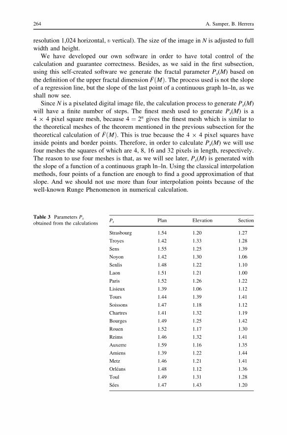
Since N is a pixelated digital image file, the calculation process to generate Ps(M)

will have a finite number of steps. The finest mesh used to generate Ps(M) is a

4 9 4 pixel square mesh, because 4 ¼ 2n gives the finest mesh which is similar to

the theoretical meshes of the theorem mentioned in the previous subsection for the

theoretical calculation of �F Mð Þ. This is true because the 4 9 4 pixel squares have

inside points and border points. Therefore, in order to calculate Ps(M) we will use

four meshes the squares of which are 4, 8, 16 and 32 pixels in length, respectively.

The reason to use four meshes is that, as we will see later, Ps(M) is generated with

the slope of a function of a continuous graph ln–ln. Using the classical interpolation

methods, four points of a function are enough to find a good approximation of that

slope. And we should not use more than four interpolation points because of the

well-known Runge Phenomenon in numerical calculation.

Table 3 Parameters Ps

obtained from the calculationsPs Plan Elevation Section

Strasbourg 1.54 1.20 1.27

Troyes 1.42 1.33 1.28

Sens 1.55 1.25 1.39

Noyon 1.42 1.30 1.06

Senlis 1.48 1.22 1.10

Laon 1.51 1.21 1.00

Paris 1.52 1.26 1.22

Lisieux 1.39 1.06 1.12

Tours 1.44 1.39 1.41

Soissons 1.47 1.18 1.12

Chartres 1.41 1.32 1.19

Bourges 1.49 1.25 1.42

Rouen 1.52 1.17 1.30

Reims 1.46 1.32 1.41

Auxerre 1.59 1.16 1.35

Amiens 1.39 1.22 1.44

Metz 1.46 1.21 1.41

Orleans 1.48 1.12 1.36

Toul 1.49 1.31 1.28

Sees 1.47 1.43 1.20


Then (see Fig. 5), our software generates a square mesh, which we have called

g5, consisting of 32 9 h5 square boxes with an edge dimension

a5 ¼ 1; 024�2�5 ¼ 32pixels. Then we apply that mesh on the image of N and we

calculate ln(s5), where s5 is the number of boxes of g5 which have black pixels.

Then we repeat the process with the other square meshes g6; g7 and g8 having

64 9 h6, 128 9 h7, 256 9 h8 square boxes, respectively. The edge dimensions are

a6 ¼ 1; 024� 2�6 ¼ 16; a7 ¼ 1; 024�2�7 ¼ 8 and a8 ¼ 1; 024�2�8 ¼ 4, respec-

tively (see Fig. 5). Then we calculate lnðs6Þ; lnðs7Þ and lnðs8Þ, where s6; s7 and s8

are the number of boxes with black pixels in each mesh g6; g7 and g8, respectively.

For example, Table 1 shows the data corresponding to Fig. 5: (h5; h6; h7; h8 = (32,

64, 128, 256), (s5, s6, s7, s8) = (799, 2689, 8236, 22294).

As a result of the above mentioned process we obtain the coordinates of four

points ðlnð25Þ; lnðs5ÞÞ; ðlnð26Þ; lnðs6ÞÞ; ðlnð27Þ; ðlnðs7ÞÞ; ðlnð28Þ; lnðs8ÞÞ in a graph

ln–ln.

Figure 6 shows the four points which result from Table 1. Now, our software

calculates the slope of the continuous graph ln–ln on the fourth point [ln(28), ln(s8)].

Such slope is an extrapolation of the process used to calculate the theoretical limit of

the upper fractal dimension �F Mð Þ. To confirm that the preceding claim is true, you

can consider ln 2nð Þ ¼ x; lnðsnÞ ¼ f ðxÞ; lnðsnÞlnð2nÞ ¼

f ðxÞx

and use l’Hopital’s rule. In order

to calculate that slope, the software implements the classical four-point formula

Table 4 Parameters Pr

obtained from the calculationsPr Plan Elevation Section


Troyes 1.52 1.54 1.46

Sens 1.53 1.46 1.60

Noyon 1.52 1.50 1.46

Senlis 1.54 1.41 1.52

Laon 1.59 1.55 1.39

Paris 1.53 1.61 1.41

Lisieux 1.42 1.41 1.29

Tours 1.50 1.58 1.51

Soissons 1.45 1.55 1.32

Chartres 1.56 1.50 1.43

Bourges 1.54 1.52 1.63

Rouen 1.47 1.60 1.43

Reims 1.53 1.63 1.52

Auxerre 1.52 1.52 1.47

Amiens 1.46 1.58 1.61

Metz 1.44 1.48 1.58

Orleans 1.49 1.54 1.36

Toul 1.49 1.56 1.48

Sees 1.51 1.58 1.45


y0

3 ’ 16hð�2y0 þ 9y1 � 18y2 þ 11y3Þ, where h ¼ ln2 and yi ¼ lnðs5þiÞ. The final

result y30 given by our software is the fractal parameter Ps(M). In the example used

in Fig. 5, the fractal parameter is 16 ln 2ð�2 lnð799Þ þ 9 lnð2689Þ � 18 lnð8236Þþ

11 lnð22294ÞÞ ’ 1:33.

Variants of the Fractal Parameter

We have explained that the fractal parameter Ps(M) is generated by means of the

slope in the fourth point of the continuous graph ln–ln. However, in the theoretical

cases of fractal self-similar objects such a graph is a straight line. Therefore, if we

generate a fractal parameter under the hypothesis of self-similarity, then we can use

the slope of the regression line corresponding to the discrete set of the four points

belonging the graph ln� ln. So, the calculation is the quotient of the covariancesrxy

rxx

where rxy ¼ 14

Pi¼4i¼0 ðyi � �yÞðð5þ iÞ ln 2� �xÞ; rxx ¼ 1

4

Pi¼4i¼0 ðð5þ iÞ ln 2� �xÞ2; �x ¼

5þ6þ7þ84

ln 2; �y ¼ y0þy1þy2y3

4. This fractal parameter will be called Pr(M). In the case

of the rose window displayed in Fig. 5, we have Pr(M) ^ 1.60.

Some commercial software like Benoit 1.31, by TruSoft Int’l Inc, allow

generation of Pr(M) from the pixel file N. In this situation, of course, the value

PrðMÞ obtained with our software is the same as the value obtained with Benoit.

When many calculation steps are used, with more meshes, commercial software

always uses the slope of the regression line. For instance, Benoit 1.31 uses 22

Table 5 Parameters Pb

obtained from the calculationsPb Plan Elevation Section

Strasbourg 1.60624 1.57518 1.49741

Troyes 1.60898 1.51084 1.44870

Sens 1.61128 1.48047 1.52771

Noyon 1.59964 1.49272 1.74688

Senlis 1.62527 1.44926 1.48583

Laon 1.63119 1.52501 1.41866

Paris 1.63493 1.56197 1.40060

Lisieux 1.53833 1.41831 1.36375

Tours 1.59779 1.56567 1.49519

Soissons 1.55476 1.46949 1.34814

Chartres 1.59455 1.48041 1.45659

Bourges 1.62432 1.52556 1.56154

Rouen 1.57932 1.55053 1.51279

Reims 1.61244 1.59039 1.50352

Auxerre 1.61642 1.49271 1.47486

Amiens 1.56189 1.54350 1.56477

Metz 1.54586 1.49182 1.51680

Orleans 1.58828 1.50319 1.42449

Toul 1.58842 1.54721 1.44217

Sees 1.59304 1.53743 1.44756


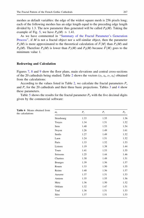
meshes as default variables: the edge of the widest square mesh is 256 pixels long;

each of the following meshes has an edge length equal to the preceding edge length

divided by 1.3. The new parameter thus generated will be called Pb(M). Taking the

example of Fig. 5, we have Pb(M) ^ 1.41.

As we have commented in ‘‘Summary of the Fractal Parameter’s Generation

Process’’, if M is not a fractal object nor a self-similar object, then the parameter

Ps(M) is more approximated to the theoretical calculation of �F Mð Þ than Pr(M) and

Pb(M). Therefore Ps(M) is lower than Pr(M) and Pb(M) because �F Mð Þ goes to the

minimum value 1.

Redrawing and Calculation

Figures 7, 8 and 9 show the floor plans, main elevations and central cross-sections

of the 20 cathedrals being studied. Table 2 shows the vectors (s5; s6; s7; s8Þ obtained

from the calculations:

According to the values listed in Table 2, we calculate the fractal parameters Ps

and Pr for the 20 cathedrals and their three basic projections. Tables 3 and 4 show

these parameters.

Table 5 shows the results for the fractal parameter Pb with the five decimal digits

given by the commercial software:

Table 6 Means obtained from

the calculationsmi Ps Pr Pb


Troyes 1.34 1.51 1.52

Sens 1.40 1.53 1.54

Noyon 1.26 1.49 1.61

Senlis 1.27 1.49 1.52

Laon 1.24 1.51 1.52

Paris 1.33 1.52 1.53

Lisieux 1.19 1.38 1.44

Tours 1.41 1.53 1.55

Soissons 1.25 1.44 1.46

Chartres 1.30 1.49 1.51

Bourges 1.39 1.56 1.57

Rouen 1.33 1.50 1.55

Reims 1.40 1.56 1.57

Auxerre 1.37 1.51 1.53

Amiens 1.35 1.55 1.56

Metz 1.36 1.50 1.52

Orleans 1.32 1.47 1.51

Toul 1.36 1.51 1.53

Sees 1.37 1.51 1.53


Results and Discussion

Fractal geometry has often been used to study certain elements of architecture, but

this is the first time that it has been used to find a new geometric pattern in the

French Gothic architecture.

After studying the 20 most important French Gothic cathedrals, in the preceding

section of this paper, we have found the means of their respective floor plans, main

elevations and center cross-sections. Table 6 shows the means msi; mri and mbi,

expressed with two decimal digits, for the fractal parameters Ps; Pr and Pb,

respectively.

We will show that the fractal parameters Pr and Pb in Table 6 have a very strong

linear correlation among them, so we can consider the fractal parameters Ps and Pr

only. From Table 6 we can see that the total mean mr of the data from Pr is

mr ^ 1.50 and the total mean mb of the data from Pb is mb ’ 1:53. The standard

deviation of the 20 results from Table 6 is rr ^ 0.041 for Pr, and rb ^ 0.037 for

Pb. The covariance between the results for Pr and the results for Pb is rrb ^ 0.0012.

Therefore, the Pearson correlation coefficient between the two sets of results is

Rrb ¼ rrb

rrrb’ 0:80, and the Pearson determination coefficient between the two sets of

results is Rrb2 ^ 0.63. Using Student’s t test with 20–2 degrees of freedom and eight

decimal digits (we use eight decimal digits because we want to show the real

magnitude of the probability) we reject the null hypothesis of ‘‘no correlation

between the two sets of results’’ with a probability Prb ^ 0.99998620. Therefore, in

order to study the fractal pattern we will only use the data sets Pr and Ps in Table 6.

Now we will prove that the 20 means msi from Table 6, corresponding to Ps, are

very concentrated around their total mean ms ^ 1.33. To that effect, we calculate

the standard deviation of these 20 results, which is rs ^ 0.058, and the variance

rs20.0034. Therefore, Pearson’s coefficient of variation r

mis 4 %. In general, when

the Pearson coefficient of variation is under 25 % it is considered that there is little

scattering around the mean. Since the coefficient in this case is 4 %, we conclude

that the total mean ms is highly representative and shows very little scattering.

Next, we claim that the total mean ms is a non-random result. To test this claim

we will use the well-known Pearson’s Chi squared test, and we use eight decimal

digits because we want to show the real magnitude of the probability of being a non-

random result. We apply Pearson’s Chi squared test with 19 degrees of freedom in

the following two-way table (Table 7): I1 ¼ ½1:01; 1:05�; I2 ¼ ½1:06; 1:10�; . . .; I19 ¼½1:91; 1:95�; I20 ¼ ½1:96; 2�; f1;k ¼ 0; f2;k ¼ 20 are the obtained frequencies, with the

following exceptions: f1,4 = f1,9 = 1, f1,5 = 2, f1,6 = 3, f1,7 = 6, f1,8 = 7,

Table 7 Two-way table of ms

I1 I2 I3 I4 I5 I6 I7 I8 I9 I10 . . . I20 Total

msi 2 Ik 0 0 0 1 2 3 6 7 1 0 . . . 0 20

msi 62 Ik 20 20 20 19 18 17 14 13 19 20 . . . 20 380

Total 20 20 20 20 20 20 20 20 20 20 . . . 20 400


f2,4 = f2,9 = 19, f2;5 = 18, f2,6 = 17, f2,7 = 14, f2,8 = 13; and F1;k ¼ 400400

, F2;k ¼7;600400

are the expected frequencies. Consequently, applying Pearson’s Chi squared

test with 19 degrees of freedom we conclude that Table 7 is a non-random table,

because the probability of being non-random is P ’ 0:99999999.

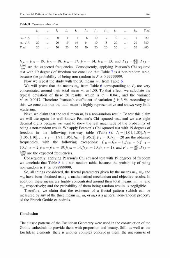
Now we repeat the study with the 20 means mri from Table 6.

We will prove that the means mri from Table 6 corresponding to Pr are very

concentrated around their total mean mr ’ 1:50. To that effect, we calculate the

typical deviation of these 20 results, which is rr ¼ 0:041, and the variance

r2 ^ 0.0017. Therefore Pearson’s coefficient of variation rm

is 3 %. According to

this, we conclude that the total mean is highly representative and shows very little

scattering.

Next, we claim that the total mean mr is a non-random result. To test this claim

we will use again the well-known Pearson’s Chi squared test, and we use eight

decimal digits because we want to show the real magnitude of the probability of

being a non-random result. We apply Pearson’s Chi squared test with 19 degrees of

freedom in the following two-way table (Table 8): I1 ¼ ½1:01; 1:05�; I2 ¼½1:06; 1:10�; . . .; I19 ¼ ½1:91; 1:95�; I20 ¼ ½1:96; 2�; f1;k ¼ 0; f2;k ¼ 20 are the obtained

frequencies, with the following exceptions: f1;8 ¼ f1;9 ¼ 1; f1;10 ¼ 6; f1;11 ¼10; f1;12 ¼ 2; f2;8 ¼ f2;9 ¼ 19; f2;10 ¼ 14; f2;11 ¼ 10; f2;12 ¼ 18; and F1;k ¼ 400

400;F2;k ¼

7;600400

are the expected frequencies.

Consequently, applying Pearson’s Chi squared test with 19 degrees of freedom

we conclude that Table 8 is a non-random table, because the probability of being

non-random is P ^ 0.99999999.

So, all things considered, the fractal parameters given by the means mri, msi and

mbi have been obtained using a mathematical mechanism and objective results. In

addition, these means are highly concentrated around their total means, ms, mr and

mb, respectively; and the probability of them being random results is negligible.

Therefore, we claim that the existence of a fractal pattern (which can be

measured by any of the three means ms, mr or mb) is a general, non-random property

of the French Gothic cathedrals.

Conclusion

The classic patterns of the Euclidean Geometry were used in the construction of the

Gothic cathedrals to provide them with proportion and beauty. Still, as well as the

Euclidean elements, there is another complex concept in them: the unevenness of

Table 8 Two-way table of mr

I1 . . . I7 I8 I9 I10 I11 I12 I13 . . . I20 Total

mri 2 Ik 0 . . . 0 1 1 6 10 2 0 . . . 0 20

mri 62 Ik 20 . . . 20 19 19 14 10 18 20 . . . 20 380

Total 20 . . . 20 20 20 20 20 20 20 . . . 20 400


their structures, which determines their space-filling ability, i.e. their level of

roughness. The best tool to describe this concept is given by Fractal Geometry, by

means of a ratio called fractal dimension. In this paper we use this concept to

generate fractal parameters which give a measure of roughness. These parameters

are not only attributable to Euclidean elements, but also given by the final

architectural result of the constructions.

The 20 cathedrals being studied in this paper are a highly representative sample

of the French Gothic style, one which prevents arbitrariness. By means of this

sample, we analyze the geometry of the resulting construction using new parameters

which were unknown until now. Since each construction had its very own

authorship and circumstances, we have not gone on to compare cathedrals with each

other. Instead, we have examined if the design traits and structures of these

constructions have a deeper geometrical sense than was known to us yet.

In this paper we prove that the French Gothic cathedrals do not only follow the

Euclidean geometric patterns, but also have another characteristic pattern which is

determined by fractal parameters.

We conclude the existence of a general non-random pattern within the fractal

dimension of the French Gothic cathedrals.

References

Baldellou, M. 1995. Catedrales De Europa. Madrid: Espasa Calpe. (in Spanish).

Batty, M., and P. Longley. 2001. The fractal city. In AD, Urban Environments, ed. E.G. Mapelli. New

York: Wiley.

Bechhoefer, W., and C. Bovill. 1994. Fractal analysis of traditional housing in Amasya, Turkey.

Traditional Dwellings and Settlements Working Paper Series 61:1–21.

Bechmann, R. 1985. Villard de Honnecourt. La Pensee Technique au XI-Iie Siecle et sa Communication.

Paris: Picard Editeur. (in French).

Bovill, C. 1996. Fractal geometry in architecture and design. Boston: Birkhauser.

Bovill, C. 2008. The doric order as a fractal. Nexus Network Journal 10:283–290.

Brown, C.T., and W.R.T. Witschey. 2003. The fractal geometry of ancient Maya settlement. Journal of

Archaeological Science 30:1619–1632.

Burkle-Elizondo, G. 2001. Fractal geometry in Mesoamerica. Symmetry. Culture and Science

12:201–214.

Cooper, J. 2003. Fractal assessment of street-level skylines: a possible means of assessing and comparing

character. Urban Morphology 7:73–82.

Crompton, A. 2002. Fractals and picturesque composition. Environment Planning B 29:451–459.

Edgar, G. 1998. Integral, probability, and fractal measures. New York: Springer.

Eglash, R. 1999. African fractals: modern computing and indigenous design. New Brunswick: Rutgers

University Press.

Falconer, K.J. 1990. Fractal geometry, mathematical foundations and applications. Chichester: Willey.

Falconer, K.J. 1997. Techniques in fractal geometry. Chichester: Willey.

Hammer, J. 2006. From fractal geometry to fractured architecture: the Federation Square of Melbourne.

Mathematical Intelligencer 28:44–48.

Joye, Y. 2007. Fractal architecture could be good for you. Nexus Network Journal 9:311–320.

Kunst, H., and W. Schekluhn. 1996. La Catedral de Reims. Madrid: Siglo Veintiuno. (in Spanish).

Murray, S. 1996. Notre-Dame, Cathedral of Amiens, the power of change in Gothic. Cambridge:

University of Cambridge.

Ostwald, M.J. 2001. Fractal architecture: late 20th century connections between architecture and fractal

geometry. Nexus Network Journal 3:73–84.


Ostwald, M.J. 2010. The politics of fractal geometry in Russian paper architecture: the intelligent market

and the cube of infinity. Architecture Theory Review 15:125–137.

Ostwald, M.J., and J. Vaughan. 2009. Calculating visual complexity in Peter Eisenman’s architecture: a

computational fractal analysis of five houses (1968–1976). CAADRIA 2009: Proceedings of the

Fourteenth Conference on Computer Aided Architectural Design Research in Asia, 75–84.

Ostwald, M.J., and J. Vaughan. 2010. Comparing Eisenman’s House VI and Hejduk’s House 7: a

mathematical analysis of formal complexity in plan and elevation. Aesthetics and design: 21st

Biennial Congress of IAEA. Dresden: Technische Universitat.

Ostwald, M.J., and J. Vaughan. 2013. Representing architecture for fractal analysis: a framework for

identifying significant lines. Architectural Science Review 56(3):242–251.

Ostwald, M.J., Vaughan, J., and S. Chalup. 2008. A computational analysis of fractal dimensions in the

architecture of Eileen Gray. Biological processes and computation: Proceedings of the 28th Annual

Conference of the Association for Computer Aided Design in Architecture (ACADIA), 256–263.

Prache, A. 2000. Cathedrals of Europe. Cornell: University Press.

Rian, I.M., J.H. Park, H.U. Ahn, and D. Chang. 2007. Fractal geometry as the synthesis of Hindu

cosmology in Kandariya Mahadev temple, Khajuraho. Building and Environment 42: 4093–4107.

Sala, N. 2006. Fractal geometry and architecture: some interesting connections. WIT Transactions on The

Built Environment 86:163–173.

Schutz, B. 2008. L’art des Grandes Cathedrales. Paris: Hazan. (in French).

Simon, O. 1985. La Catedral gotica. Madrid: Alianza Editorial. (in Spanish).

Toman, R. 1998. El Gotico. Arquitectura, Escultura y Pintura. Paris: Konemann. (in Spanish).

Vaughan, J., and M.J. Ostwald. 2009. A quantitative comparison between the formal complexity of Le

Corbusier’s Pre-Modern (1905–1912) and Early Modern (1922–1928) architecture. Design

Principles and Practices: An International Journal 3:359–372.

Vaughan, J., and M.J. Ostwald. 2010. Using fractal analysis to compare the characteristic complexity of

nature and architecture: re-examining the evidence. Architectural Science Review 53:323–332.

Vaughan, J., and M.J. Ostwald. 2011. The relationship between the fractal dimension of plans and

elevations in the architecture of Frank Lloyd Wright: comparing the Prairie Style, Textile Block and

Usonian Periods. Architecture Science ArS 4:21–44.

Wilson, C. 1990. The Gothic Cathedral, the architecture of the Great Church. London: Thames and

Hudson.

Albert Samper is an Architect who obtained his Ph.D. in Architecture at the University Rovira i Virgili

of Tarragona in 2013. Presently, he is an associate professor of Architecture at the same university and his

main fields of interest are: Fractal Geometry and the application of Geometry to Architecture.

Blas Herrera is Geometer who obtained his D.Sc. in Mathematics at the University Autonoma of

Barcelona in 1994. Presently, he is a full professor of Applied Mathematics at the University Rovira i

Virgili of Tarragona. His main fields of research interest are: Classical and Differential Geometry, and the

application of Geometry to Architecture, Fluid Mechanics and Engineering.


The Fractal Pattern of the French Gothic Cathedrals … · 2017-08-24 · The Fractal Pattern of...

Documents

Transcript of The Fractal Pattern of the French Gothic Cathedrals … · 2017-08-24 · The Fractal Pattern of...