1

The Formation of Expectations, Inflation and the Phillips Curve

Olivier Coibion UT Austin & NBER

Yuriy Gorodnichenko UC Berkeley & NBER

Rupal Kamdar UC Berkeley

March 25th , 2017

Abstract This paper argues for a careful (re)consideration of the expectations formation process and a more systematic inclusion of real-time expectations through survey data in macroeconomic analyses. While the rational expectations revolution has allowed for great leaps in macroeconomic modeling, the surveyed empirical micro-evidence appears increasingly at odds with the full-information rational expectation assumption. We explore models of expectation formation that can potentially explain why and how survey data deviate from full-information rational expectations. Using the New Keynesian Phillips curve as an extensive case study, we demonstrate how incorporating survey data on inflation expectations can address a number of otherwise puzzling shortcomings that arise under the assumption of full-information rational expectations. Keywords: Expectations, Inflation, Surveys JEL Codes: E3, E4, E5

1. Introduction Macroeconomists have long recognized the central role played by expectations: nearly all economic

decisions contain an intertemporal dimension such that contemporaneous choices depend on agents’

perceptions about future economic outcomes. How agents form those expectations should therefore play a

central role in macroeconomic dynamics and policy-making. While full-information rational expectations

(FIRE) have provided the workhorse approach for modeling expectations for the past few decades, the

increasing availability of detailed micro-level survey-based data on subjective expectations of individuals

has revealed that expectations deviate from FIRE in systematic and quantitatively important ways including

forecast-error predictability and bias.

2

How should we interpret these results from survey data? In this paper, we tackle this question by

first reviewing the rise of the FIRE assumption and some of the successes that it has achieved. We then

discuss the literature testing the FIRE assumption, focusing particularly on more recent work exploiting

detailed micro-level survey data that has become increasingly available. This growing body of work

documents pervasive departures from the FIRE assumption, especially when looking at the beliefs of

households or managers. Given these differences between the traditional assumption of FIRE and the

empirical evidence on how agents form their expectations, we then review the range of theoretical models

that have been proposed to account for the observed deviations from FIRE, as well as some of the empirical

evidence specifically testing these models.

We focus in particular on inflation expectations and their role in the Phillips curve. Our emphasis

on inflation expectations rather than expectations of other macroeconomic variables reflects both their

greater availability in survey data as well as their unique importance in macroeconomics. The crucial role

played by inflation expectations on aggregate outcomes and policy decisions was highlighted by Fed

Chairman Greenspan,1 “I am not saying what [inflation expectations] is a function of. We know it’s a very

difficult issue, but that is the key variable. It’s important, but just because we can’t make a judgment as to

what these driving forces are in an econometric sense doesn’t mean that it’s not real.” [italics added]

The role of expectations in the context of the Phillips curve has of course long been emphasized,

going back to Friedman (1968) and Phelps (1967). While the Phillips curve began as an empirical

correlation between wage inflation and unemployment in Phillips (1958), today the workhorse version of

the relationship is the micro-founded New Keynesian Phillips curve (NKPC) that characterizes current

inflation as a function of firms’ expectations about future inflation and economic slack. Over the years,

research on the NKPC has identified a number of shortcomings such as the need for ad-hoc lags in

estimation to generate persistence in inflation, instability or a flattening of the curve, missing disinflation

during the Great Recession, inferior forecasting relative to naïve alternatives, and sensitivity to the slack

variable employed; see Mavroeidis et al. (2014) for a recent survey. These puzzles have resulted in

declarations of the death of the Phillips curve (e.g., Hall 2013).

However, the prognosis for the Phillips curve may be less grim after allowing for deviations from

FIRE. That is, employing subjective expectations gathered from surveys in the estimation of expectations-

augmented Phillips curve alleviates many of the previously identified puzzles.2

The remainder of the paper proceeds as follows. The next section will discuss the development of

FIRE from Muth (1961), the rational expectations “revolution”, and the assumption’s current proliferation

1 The Federal Open Market Committee meeting transcript from 7/5-6/1994. 2 Crump et al. (2015) similarly note that conditioning on survey data of households’ inflation expectations helps address puzzles associated with typical estimates of consumption Euler equations.

3

both inside and outside of macroeconomics. Section 3 reviews evidence that tests the null of FIRE using

survey data. In Section 4, models of expectation formation are discussed that may account for the deviations

between survey expectations and rational expectations. Section 5 provides a detailed case study on the

importance of careful consideration of the expectation formation in the case of the Phillips curve. We

discuss the strengths and empirical limitations of the FIRE-based Phillips curve. Then wide-ranging

evidence, inclusive of our own empirical analysis, is presented to demonstrate how conditioning on the

real-time expectations of economic agents (based on survey measures) can address many of the documented

limitations of the Phillips curve. We conclude in Section 6 with a call for careful consideration of

expectation formation processes, additional measurement of expectations to address the shortcomings of

currently available survey data, and an increase in usage of survey data in future research.

2. Let There Be FIRE

The expectations of agents are of integral importance in many macroeconomic models and have been

emphasized as far back as Keynes’ General Theory, where he provided a motivation for how and why

expectations may affect macroeconomic variables. Over the years, economists have continued to

incorporate expectations into their models and early attempts to model the expectation formation process

yielded alternatives such as adaptive expectations (expectations based on lagged experience) and rational

expectations (expectations are ‘model-consistent’). Today, the workhorse expectation process assumed by

macroeconomists is that of FIRE.

Muth (1961) was the first to suggest that expectations are the same as the appropriate economic

theory, or ‘model-consistent’. Muth’s proposal was not met with great excitement, and many continued to

use adaptive expectations. It was not until a decade later that the rational expectations ‘revolution’ began.

Keynesian models of the 1960s typically implied that policies could forever be used to achieve

lower unemployment and higher output at the cost of higher inflation. The stagflation experience of the

1970s, however, led many to conclude that a complete rethinking of macroeconomic models was needed.

Lucas was at the forefront of this task and the rational expectation revolution. He began with Lucas (1972)

in which an islands model was proposed where policy makers are unable to systematically exploit the

Phillips curve relationship to control the real economy. Then, Lucas (1976) developed what is now known

as the “Lucas critique”: using Keynesian models with parameters calibrated to past experience is an invalid

way to evaluate changes in government policy. In particular, if policy is altered, the way expectations are

formed changes, and if expectations affect economic outcomes then outcomes estimated using a model

calibrated with a different policy regime are inaccurate. Finally, Lucas and Sargent (1979) forcefully argued

that Keynesian economic models should be abandoned in favor of equilibrium models characterized by

4

agents with rational expectations, reacting to policy changes in a way that optimizes their personal interests

so that analysis is not subject to the Lucas critique.

From relative obscurity, the rational expectations assumption has become ubiquitous in

macroeconomic models. Examples include the efficient markets hypothesis, the permanent income theory

of consumption, and housing investment and price appreciation models. Furthermore, policy makers have

often relied on versions of rational expectations in modeling expectations. For instance, variants of

macroeconomic models employed at the Federal Reserve Board, Bank of Canada, and the International

Monetary Fund have used rational expectations (Brayton et al. 1997, Dorich et al. 2013).3

One early and enduring use of rational expectations has been in the Phillips curve that summarizes

a relationship between nominal and real quantities in the economy.4 The curve is a central ingredient in

macroeconomic models used by researchers and policymakers. In general, models with short-run tradeoffs

implied by the Phillips curve help generate monetary non-neutralities as documented in the empirical

literature (e.g., Christiano et. al 1999; Romer and Romer 1989; Romer and Romer 2004; Velde 2009).

Sargent (1999) provides a history of how policy makers have modeled expectations in the context of the

Phillips curve.

The development of the curve began with Phillips (1958), which described an empirical relationship

between wage rates and unemployment in the United Kingdom. Samuelson and Solow (1960), soon after

Phillips, documented a similar finding for the Unites States. The relationship was later extended to the more

general, overall price level, and other slack variables were employed (e.g., output gap, labor income share).

The Phillips curve tradeoff was assumed to be continuously exploitable by many; however, others

were unconvinced. Friedman (1968) and Phelps (1967) both argued for the natural rate hypothesis

suggesting a vertical long-run Phillips curve relationship. Their analyses highlighted the importance of

expectations in the Phillips curve. If agents are not surprised, monetary expansion may have no real effects.

Solow (1969) and Gordon (1970) set out to empirically assess if the Phillips curve allowed for long-run

tradeoffs. They estimated expectations-augmented Phillips curves under the assumption of adaptive

expectations. Their findings suggested that although policies that maintain low unemployment lead to

higher inflation and inflation expectations, these policies could be sustainable. It was not until the stagflation

of the 1970s and the Lucas (1972) and Sargent (1971) critiques of the Solow and Gordon tests, that the long-

run tradeoff beliefs were abandoned and the importance of inflation expectations accepted.

3 There are also variants of these macroeconomic models that employ other expectation formation processes. The FRB/US used by the Federal Reserve can either use rational expectations or expectations formed using a small VAR (Brayton et al. 1997). The Bank of Canada’s Terms-of-Trade Economic Model (ToTEM) originally modeled firms and households as rational. In 2011, the Bank of Canada updated to ToTEM II which allows for rule of thumb firms and households (Dorich et al. 2013). 4 For a thorough history of the Phillips curve see King (2008) and Gordon (2011). The former focuses on the use of the Phillips curve in policy and the latter highlights the different schools of thought on the Phillips curve post-1975.

5

After Lucas (1972), which relied on imperfect information, macroeconomists set out to incorporate

sticky prices and wages into rational expectation models.5 Some assumed prices or wages were set in a prior

period and chosen so that the expectation of demand equaled the expectation of supply. Fischer (1977), Gray

(1976), and Phelps and Taylor (1977) take this expected market clearing approach. A shortcoming of this

method—as well as Lucas’ island model—is that the persistence of macroeconomic shocks could only be as

long as the longest lead at which prices or wages were being set. Others utilized staggered contract models

that better capture the stylized facts of firm price-setting behavior (price and wage setting is staggered with

not all firms changing simultaneously, and prices and wages are fixed for long periods of time). Taylor (1979,

1980) developed the staggered pricing model with fixed duration. Firms in his models pick their prices for

N>1 periods, also known as the contract period. In each period, 1/N firms pick their new price, a function of

past and future price choices of other firms. The backward-looking component of the price choice of firms is

able to generate persistence. As an alternative to constant duration staggered pricing, Calvo (1983) introduced

random duration staggered pricing. He assumed that a firm faced a constant probability of being allowed to

change prices in a given period. This results in i.i.d. contract lengths across firms, greatly simplifying the

algebra required in staggered price-setting models.6

As a result of these theoretical efforts, the purely forward-looking NKPC emerged as the dominant

framework. It is microfounded from the optimization problem of monopolistically competitive firms subject

to a friction limiting their price changing ability. The most common friction imposed today is that of time-

dependent sticky prices as in Calvo (1983); however, other pricing frictions such as fixed duration contracts

also suffice. Similar to earlier versions of expectations-augmented Phillips curves, the NKPC underscores the

prominent role of inflation expectations in determining current inflation. However, in contrast to the earlier

work, the canonical NKPC traces the coefficients in the Phillips curve to structural parameters—hence making

the NKPC immune to the Lucas critique—and enshrines the FIRE framework thus completing the research

agenda laid out in the 1970s. Given the prominence of the NKPC as an application of rational expectations,

we use it as the primary example in our discussion henceforth.

3. Measuring Expectations: From Skepticism to Increasing Acceptance The proliferation and dominance of FIRE in macroeconomic models is due in large part to the fact that it

allows for policy analysis not subject to the Lucas critique as well as relative ease of optimization in

5 For a thorough review of the modeling of price and wage setting behavior see Taylor (1999). 6 Research has also explored state-dependent pricing where firms can change prices whenever desired but to do so must pay a fixed cost. This approach leads to Ss pricing decisions, which are generally difficult to aggregate (e.g., Golosov and Lucas 2007). Gertler and Leahy (2008) analytically develop a state-dependent pricing model with idiosyncratic shocks to firm productivity. The resulting Phillips curve is a variant of the one derived under Calvo pricing, with the main variation being the parameterization of the coefficient on output.

6

comparison to more complicated expectation formation processes. However, are rational expectations

consistent with micro-level evidence provided by survey data? There is a vast literature that tests the null

hypothesis of FIRE using a number of different procedures and data sets.7 In this section we focus on

findings related to inflation expectations in order to guide our analyses on the Phillips curve.

Although surveys can provide valuable information to answer this question, many

macroeconomists have been uncomfortable with relying on these data to inform their choice or calibration

of models. Skepticism toward survey expectations can be traced back to papers from the 1940s to 1960s

that critique survey methodologies (e.g., Machlup 1946) and found survey data not useful in predicting

individual behavior (e.g., National Bureau of Economic Research 1960; Juster 1964).8 Others argued that

only theories, not assumptions, could be empirically tested. Prescott (1977) forcefully expressed this view:

“Like utility, expectations are not observed, and surveys cannot be used to test the rational expectations

hypothesis. One can only test if some theory, whether it incorporates rational expectations or, for the matter,

irrational expectations, is or is not consistent with observations” [underlining his]. Thus, it was

commonplace for economists to view the use of survey expectations as suspect.

This perspective has become increasingly uncommon, however. Zarnowitz (1984) and Lovell (1986)

argued against the premise that assumptions should not be tested using micro data. Manski (2004) concluded

that the hostility towards surveys is based on meager evidence and suggested that survey expectations provide a

viable way to test models of the expectation formation process. If survey evidence consistently and forcefully

rejects FIRE, one may be more inclined to discount models relying on the assumption.

A number of papers have used a battery of econometric tests to investigate if survey-based expectations

are in line with FIRE.9 The literature consistently finds survey-based expectations deviate from FIRE. Jonung

and Laidler (1988) exploit a Swedish survey on contemporaneous inflation perceptions, i.e. agents’ beliefs about

current or past inflation rates, to assess rationality. In contrast to inflation expectations (which are about the

future), inflation perceptions are not subject to the “Peso problem”.10 They find, that although unbiased, errors

made by households are serially correlated. Roberts (1998) suggests that inflation expectations from the

7 For a thorough review, see Pesaran and Weale (2006). 8 See Dominitz and Manski (1997) and Manski (2004) for a history of the controversy surrounding the use of surveys as a measure for expectations. 9 As reviewed in Sheffrin (1996), there are four popular tests of rationality: (1) Unbiasedness: surveys should provide an unbiased predictor of the relevant variable; (2) Efficiency: the survey expectation should use past observations of the variable in the same way that the variable actually evolves over time; (3) Forecast-error unpredictability: the difference between the survey expectations and actual realizations should be uncorrelated with all information available at the time of forecast; (4) Consistency: given forecasts made at different times for some variable in the future, these two forecasts should be consistent with one another. 10 Suppose one is forming expectations about the value of the Mexican Peso to the U.S. Dollar, and there is a positive probability of a Peso devaluation. FIRE agents would incorporate the devaluation probability into their expectations. Assume the devaluation does not occur. Then ex-post, the ex-ante inflation expectations would appear to have a systematic error despite agents having FIRE.

7

Livingston Survey and the Michigan Survey of Consumers (MSC) have an “intermediate” level of rationality,

that is they are neither rational nor do they follow a simple autoregressive model. Croushore (1998) notes that,

over time with longer time series of survey data, survey expectations have become more in line with the

predictions of rational expectations; however, expectations still do not pass all tests for optimality and at times

are biased. Mankiw et al. (2003) use inflation expectations gathered from various surveys and demonstrate that

each survey meets and fails some of the requirements of rationality. Croushore (1993, 1997) provide an overview

of rationality tests that have used the Survey of Professional Forecasters (SPF) and Livingston data.

In addition to the canonical econometric tests, one can also assess if FIRE hold in subsamples of

the population. Of course, while this does not invalidate the possibility that FIRE may hold in the aggregate,

it does provide qualitative evidence that agents may not be fully informed. Some have noted the existence

of demographic biases in inflation expectations. Bryan and Venkatu (2001) note that women tend to have

higher inflation expectations even after controlling for race, education, marital status, income, and age.

Souleles (2004) finds consumer demographics are correlated with inflation forecast errors in the MSC.

Bruine de Bruin et al. (2010) highlight how inflation expectations are higher among those with lower

financial literacy. Similarly, experiences, and therefore age, may also affect inflation expectations.

Malmendier and Nagel (2016) document that learning from experience, that is overweighting the inflation

experienced during one’s own lifetime, appears to occur in the MSC.

One striking feature of survey data is that it reveals dramatic differences across individuals in terms

of their perceived (past) inflation rates. For example, Jonung (1981) found in a survey of Swedish

households that differences in households’ perceptions about recent inflation were almost as large as

differences in their expectations of future inflation, and that households’ beliefs about recent inflation were

a strong predictor about their beliefs over future inflation. Kumar et al. (2015) document similar patterns

for households and firms managers in New Zealand. Large differences in perceptions of recent inflation

across economic agents are striking because they are strongly at odds with the common assumption of fully-

informed agents. Subsequent work has documented properties of inflation perceptions and how these relate

to differences in inflation expectations.

Building on Jonung’s (1981) finding that women had a higher perceived past inflation rate than

men in 1977 because women purchased a larger share of food and food price inflation in 1977 was higher

than that of general inflation, others have shown that an individual’s consumption basket affects his or her

perception of inflation. Georganas et al. (2014) conduct a financially incentivized experiment amongst

consumers and find that perceived inflation rates are biased towards goods frequently bought. Ranyard et

al. (2008) note that the expenditure-weighting in the CPI calculation results in measured inflation being a

better representation of inflation experienced by households in the upper percentiles of the expenditure

distribution than those that are less wealthy. Coibion and Gorodnichenko (2015a) find that households in

8

groups that purchase gasoline more frequently adjust their inflation forecasts by more when oil prices

change than do other households. Cavalho et al. (2016) document that consumers use their memories of

supermarket prices when forming their inflation expectations. Johannsen (2014) finds that low-income

households experience more dispersion in changes of their cost-of-living and also display more

heterogeneity in their inflation forecasts.

Others have discussed how the accuracy and dispersion of inflation expectations may vary over

time. Some have noted that the accuracy of inflation expectations varies with the business cycle. Carvalho

and Nechio (2014) find that many households form their forecasts in a way that is consistent with a Taylor

rule on the part of monetary policymakers, but that this is primarily true during downturns. Coibion and

Gorodnichenko (2015b) also find that deviations from FIRE in the U.S. decline during downturns, as do

Loungani et al. (2013) in a much wider cross-section of countries. Others have empirically demonstrated

and modeled how the amount of disagreement in inflation expectations may vary over time. Cukierman and

Wachtel (1979) and Mankiw et al. (2003) empirically demonstrate that a high dispersion of inflation

expectations is positively correlated with a high level of inflation and with a high variance in recent

inflation.11

Recap: Early suspicion of directly measuring expectations has subsided over the years, and economists are

increasingly conducting surveys and relying on survey data. Survey-based expectations have been used to

test the assumption of FIRE, and the literature consistently finds deviations from FIRE. Surveys reveal

demographic biases across gender and age; perceived inflation is affected by an individual’s consumption

basket; and the accuracy and dispersion of expectations may vary systematically over time. These

characteristics suggest that assuming agents hold FIRE may be too strong. At the same time, Croushore

(2010) finds that while departures from rational expectations over short periods of time can be frequent and

large, these departures tend to dissipate over longer periods. Thus, expectations appear to converge to FIRE

over time. Coming to grips with these different empirical findings requires developing models of the

expectations formation process that go beyond FIRE.12

4. Alternatives to FIRE

11 Capistrán and Timmerman (2009) offer an alternative explanation within the FIRE framework. They develop a model of asymmetric costs to over- and under-predicting, heterogeneous loss functions amongst agents, and a constant loss component to try to fit the observed characteristics of SPF inflation forecasts without deviating from FIRE. However, Coibion and Gorodnichenko (2012) show that this type of model makes counterfactual predictions for the dynamic responses of forecast errors to shocks. 12 The evidence discussed in this section need not invalidate the usage of FIRE in all cases when one is interested in aggregate outcomes and arbitrage opportunities are not costly. For example, consider financial markets where some traders are rational while others are not. With sufficient resources and an appropriate institutional environment, rational agents could arbitrage away market outcomes that are not rational resulting in the aggregates being effectively set using FIRE.

9

As documented in the previous section, the empirical evidence generally rejects the FIRE assumption. How

should one interpret these deviations? Do they imply that expectations are irrational? Or do they reflect

constraints on the information processing capacity of economic agents? Does it matter? And, importantly,

how should we model the expectation formation process? As Shiller (1978) noted early in the rational

expectations revolution, “Even when we do have survey data or other data which purport to represent

expectations, if these expectations are endogenous in our model then we still must model the determination

of these expectations.”

Most recent work in this direction has emphasized possible deviations from full-information due to

information rigidities while maintaining the assumption of rational expectations. One such approach is the

sticky information approach of Mankiw and Reis (2002), in which agents update their information sets

infrequently but when they do so, they acquire FIRE. Carroll (2003) helps rationalize the sticky information

approach by suggesting that information is transferred from professional forecasters to consumers over time

via the news. An alternative approach, often called noisy information or rational inattention, is motived by

information processing constraints of agents. The information constraints are modeled as agents either

receiving noisy signals (agents observe the true values with some error) or agents rationally choosing what

information to pay attention to subject to some information constraint. Woodford (2002) takes the first

approach and Sims (2003) and Maćkowiak and Wiederholt (2009) take the latter.

Sticky information, noisy information, and rational inattention models make some common

predictions. First, the mean forecast across agents of a macroeconomic variable will under-respond relative to

the actual response of the variable after a macroeconomic shock. For example, if a shock raises inflation for

a number of periods, the mean forecast of inflation in both models will not rise by as much as actual inflation.

In sticky information, this is because some agents will be unaware that the shock has occurred and will not

change their forecast at all. In noisy information models, agents will receive signals pointing to higher inflation

but they will adjust their forecasts only gradually because of their initial uncertainty as to whether the higher

signals represent noise or true innovations. In rational inattention models, some agents will not be paying

complete attention to incoming inflation data and will not sufficiently increase their forecasts. Coibion and

Gorodnichenko (2012) document that, consistent with models of information rigidities, survey forecasts of

inflation under-respond to different macroeconomic shocks. These results obtain for a variety of surveys,

including the SPF, the Livingston Survey, FOMC member forecasts, and the MSC. Furthermore, the implied

levels of information rigidity are economically large, pointing to important deviations from FIRE.

Another common prediction from these models is that mean ex-post forecast errors across agents

will be predictable on average using ex-ante revisions in mean forecasts, in contrast to the prediction from

FIRE that ex-post forecast errors should be unpredictable. In sticky information, this reflects the fact that

10

some agents do not update their information and so their forecasts remain unchanged, anchoring the mean

forecast to the previous period’s mean forecast. In noisy information, agents update their forecasts only

gradually because of the noise in the signal, again anchoring current forecasts to previous forecasts. In

rational inattention models, current mean forecasts will be anchored to past mean forecasts because some

agents will not be paying complete attention to the relevant variable. These mechanisms imply a gradual

adjustment in mean forecasts and therefore predictability in mean forecast errors. Coibion and

Gorodnichenko (2015b) test this prediction and find robust evidence for predictability of ex-post forecast

errors from ex-ante mean forecast revisions, consistent with these models of information rigidity. Once

again, the implied deviations from FIRE are economically large and can be found in a variety of different

surveys, such as the SPF, the MSC, financial market forecasts, and Consensus Economics forecasts for

different countries.

In addition to models that emphasize information rigidities, research has considered an array of other

possible departures from FIRE. These models fall broadly into two, sometimes overlapping, categories. One

such alternative is bounded rationality, where agents are “bounded” by model misspecification yet are

“rational” in their use of least squares (Sargent, 1999). Gabaix (2014) proposes and analyzes a “sparse max”

operator in which agents build a simplified model of the world, paying attention to only some of the relevant

variables as attention bears a positive cost in the model. This approach is motivated by the limited capacity of

agents to follow and relate macroeconomic variables. Gabaix continues by analyzing the results of consumer

demand and competitive equilibrium when agents use a sparse max operator. Of particular relevance is his

analysis of a Phillips curve in the Edgeworth Box. He shows that under a sparse max operator, each

equilibrium price level corresponds to a different real equilibrium, similar to a Phillips curve. Natural

expectations in Fuster et al. (2010) is a related concept in the sense that it is a middle ground between rational

expectations and naïve intuitive expectations. Agents with natural expectations use simple, misspecified

models to forecast a complex reality.

A similar approach where agents have misspecified models is that of diagnostic expectations. This

type of expectations is motivated by Kahneman and Tversky’s (1972) representativeness heuristic that

characterizes our non-Bayesian tendency to overestimate the probability of a trait in a group when that trait

is representative or diagnostic to that group (e.g., red hair among the Irish). Gennaioli and Shleifer (2010)

and Bordalo et al. (2016) take this behavioral intuition and formalize it into diagnostic expectations. Agents

with diagnostic expectations overweight future outcomes that become more likely with incoming data.

Bordalo et al. (2016) show that diagnostic expectations in a model of credit cycles can account for stylized

facts on credit spreads such as their excess volatility, predictable reversals, and an over-reaction to news.

The second approach is to use models of learning. The most common formulation of learning is

adaptive learning where the agent acts as an econometrician in each period and uses observed outcomes to

11

estimate a perceived law of motion. From the perceived law of motion, which is not necessarily the actual

law of motion, the agent forms expectations and maximizes subject to those expectations. Evans and

Honkapohja (1999, 2012) provide an extensive review of the adaptive learning literature as well as discuss

other learning approaches. In these models, agents often observe shocks (and so in this dimension their

information is full) and have full rationality but do not know parameters governing dynamics in the

economy.

Models of learning have been used to study inflation and inflation expectations. On the theoretical

side, Orphanides and Williams (2005) demonstrate that in a model where agents use a model of finite-

memory, least squares, perpetual learning to form inflation expectations, significant and persistent

deviations of inflation expectations from those implied by rational expectations may arise. On the empirical

front, models of learning have done well matching observed inflation persistence and inflation expectation

survey data (e.g., Milani, 2007; Branch and Evans, 2006a). These empirical successes suggest learning

models may capture important deviations from FIRE.

A closely related body of work emphasizes the possibility that agents switch across different

forecasting processes over time. Branch and Evans (2006b), for example, model agents as choosing from a

list of misspecified models (parameters however are formed optimally) based on prior forecast performance.

This formulation is able to give rise to intrinsic heterogeneous expectations under suitable conditions. In

particular, with high intensities of choice (intensity of choice parameterizes the agent’s bounded rationality

and as it approaches infinity the agents approach full optimization), expectations must influence actual

outcomes. Pfajfar and Žakelj (2014) use an inflation forecasting experiment to assess the process of forecast

formation and the extent to which agents switch forecasting rules. They find that expectations are

heterogeneous with some subjects behaving in line with rational expectations while others appear to adhere

to methods of adaptive learning or trend extrapolation with frequent switching between forecasting models.

Recap: There are a variety of alternatives to FIRE that can explain why we observe pronounced and persistent

deviations from FIRE in survey data. Options include sticky information, noisy information, rational inattention,

bounded rationality, diagnostic expectations, and learning. Identifying which approach can best characterize the

expectations formation process of different agents should be a key area of future research.

5. Application: The Phillips Curve

As discussed above, FIRE often appears at odds with real-time survey-based expectations. This section

demonstrates that in a prominent and important application, the Phillips curve, incorporating real-time

expectations into the analysis can address a number of otherwise puzzling shortcomings of the NKPC that

arise under the FIRE assumption.

12

Of course, the NKPC was derived under the assumption of FIRE, and including subjective inflation

expectations is a deviation from this assumption. However, Adam and Padula (2011) show that one can use

survey expectations in the Phillips curve as long as economic agents respect the law of iterated expectations

(LIE), a weaker assumption than FIRE. This constraint is satisfied e.g. when agents are rational but not

sufficiently informed. Coibion and Gorodnichenko (2012, 2015b) and others report evidence consistent

with this condition being satisfied.

We begin with a discussion of the early successes of the NKPC and then move to the failures and

puzzles generated by the formulation. Then, survey-based expectation data availability is explored and the

literature using survey-based expectations is reviewed and shown to have solved some of the puzzles

associated with the NKPC. Our own empirical analysis confirms the importance of the inclusion of survey-

based inflation expectations in the estimation of the Phillips curve.

5.A. Successes of the Full-Information Rational Expectations Phillips Curve The expectations-augmented Phillips curve combined with the assumption that expectations are rational

and fully-informed experienced early theoretical and empirical successes.

Theoretical Success: The workhorse framework with rational expectations codified in Clarida et al. (1999)

and Woodford (2003) has been instrumental in guiding empirical analyses to link the nominal and real sides

of the economy. For example, the framework can help answer such questions as what measure of slack

(e.g., output gap, unit labor costs, unemployment) and expected inflation (e.g., one-year or one-quarter

ahead inflation, lagged or future) should be used in the Phillips curve. The framework can also provide a

benchmark to evaluate empirical estimates of Phillips curve parameters. The baseline formulation of the

curve takes the following form:

𝜋𝜋𝑡𝑡 = 𝛽𝛽𝐸𝐸𝑡𝑡𝜋𝜋𝑡𝑡+1 + 𝜅𝜅𝑋𝑋𝑡𝑡 + 𝑠𝑠ℎ𝑜𝑜𝑜𝑜𝑘𝑘𝑡𝑡 (1)

where 𝜋𝜋𝑡𝑡 is the rate of inflation at time 𝑡𝑡, 𝐸𝐸𝑡𝑡𝜋𝜋𝑡𝑡+1 is the mathematical (FIRE) expectation of inflation at

time 𝑡𝑡 + 1 given information available at time 𝑡𝑡 , 𝛽𝛽 is the discount factor, 𝑋𝑋𝑡𝑡 is the output gap (more

generally, a measure of slack in the economy), 𝜅𝜅 measures the slope of the Phillips curve and is a function

of structural parameters, 𝑠𝑠ℎ𝑜𝑜𝑜𝑜𝑘𝑘𝑡𝑡 is a “cost-push” shock.13 Note that this formulation nests the expectations-

augmented Phillips curve advocated by Friedman (1968) and Phelps (1967).

13 The most common formulation of the NKPC relates inflation to expected inflation and marginal costs. However, because the latter are not directly measurable, there has been considerable debate about what the relevant forcing term should be in the NKPC in empirical applications, as we discuss in more detail in sections 5.B and 5.C.

13

Empirical Success: Galí and Gertler (1999) and others, estimate the NKPC after imposing FIRE. Using

labor’s share of income as the forcing variable in the Phillips curve, Galí and Gertler find estimated

coefficients that conform closely to those predicted by the theory. Galí and Gertler also present a model

where some firms are forward-looking (set prices as in Calvo pricing) and some firms are backward-looking

(set prices equal to the average price set in the previous period with a correction for inflation). With these

assumptions, a hybrid Phillips curve is developed in terms of structural parameters. An estimation of the

curve is then conducted using real unit labor costs as the slack variable. The backward-looking component

is statistically significant but smaller than the forward-looking component.14 The authors conclude that the

NKPC is a reasonable approximation of inflation dynamics.

5.B. Limitations of the Full-Information Rational Expectations Phillips Curve Next, we review the empirical limitations of the Phillips curve when estimated under the assumption of

FIRE. The literature has documented the following shortcomings.

Ad-hoc lags, instability, and structural breaks: The micro-foundation of the NKPC suggests a purely

forward-looking inflation dynamics model. However, to incorporate the persistence observed in inflation

data, authors have relied on ad-hoc, backward-looking terms and estimated a “hybrid” NKPC. Fuhrer and

Moore (1995), Fuhrer (1997), Lindé (2005) and Rudd and Whelan (2005) argue that these backward-

looking components can be very important. A potential reason why this may be occurring is structural

breaks. That is, the traditional NKPC is a linearization around a zero steady state inflation rate, and it ignores

the possibility of changes in the steady state inflation rate. By doing so, the lagged terms of inflation will

spuriously capture these changes (e.g., Kozicki and Tinsley 2002; Cogley and Sbordone 2008). Mavroeidis

et al. (2014), in an earlier survey of the literature, extensively review the empirics of the NKPC with special

attention to weak identification. They conclude that estimation of the NKPC is fraught with uncertainty as

small changes in specifications can lead to large variation in point estimates due to weak identification.

Missing (dis)inflation: Several researchers have argued that inflation should have fallen much more in the

U.S. and other advanced economies during the Great Recession given the amount of slack in the economy

(e.g., Hall 2013; IMF 2013). Similarly, a missing inflation puzzle arose in real-time during the late 1990s.

Amidst a booming economy with unemployment falling below estimates of the non-accelerating inflation

14 Sheedy (2010) provides another justification for the presence of backward-looking terms. If prices that have not changed for longer periods are more likely to be changed than those set recently, the Phillips curve will have backward-looking terms even though all pricing decisions are entirely forward-looking.

14

rate of unemployment (NAIRU), policymakers disagreed about why inflation had yet to be triggered

(Meyer, 2004).15

Low out-of-sample predictive power: Atkeson and Ohanian (2001) contend that Phillips curve-based

inflation forecasts have been no more accurate than those of a naïve model where inflation next year equals

inflation in the prior year. The Phillips curve-based methods shown to be inferior are: the textbook NAIRU

Phillips curve, the Stock and Watson NAIRU model (lagged values of inflation and the slack variable are

included in this specification), and the Greenbook forecasts. Stock and Watson (2007) also find that gap-

based backward-looking Phillips curves are less successful in forecasting inflation relative to simple

univariate models after 1984.

Sensitivity to the slack variable employed: Since traditional measures of economic slack such as

unemployment and output gap yield the puzzles just described, authors have proposed the use of other slack

variables, such as the labor share of income. Overall, the results reveal sensitivity in the slope of the Phillips

curve to which slack variable is used.

Galí and Gertler (1999) argue that real unit labor cost (ulc), commonly measured by labor’s share

of income, is the superior forcing variable because of a strong contemporaneous correlation with inflation,

unlike the output gap which leads inflation. Furthermore, when estimating the Phillips curve with the output

gap as a measure of real economic conditions, the coefficient obtained is counterfactually negative and

significant, while labor’s share of income yields a positive and significant coefficient. Similarly, Woodford

(2001) and Sbordone (2002) contend unit labor cost is the best proxy for marginal costs using different

approaches. However, Rudd and Whelan (2005a) argue that neither detrended real GDP nor real unit labor

costs allow the NKPC to fit the data well. In addition, King and Watson (2012) find that since 1999, the

behavior of real unit labor costs should have implied a decline in inflation of fifteen percentage points. In

reality, actual inflation stayed relatively unchanged, allowing King and Watson to conclude, “conventional

unit labor cost measure is no longer a useful construction for inflation dynamics and has not been at least

15 Ball and Mazumder (2011), IMF (2013), Goodfriend (2004) and others argue that missing (dis)inflation could be explained by “anchored expectations.” Dräger and Lamla (2013) document that inflation expectations have become less sensitive to shocks (i.e., “anchored”) after the late 1980s. However, anchored expectations do not necessarily account for the missing (dis)inflation episodes. In the NKPC, the effect of economic slack on inflation, controlled by the coefficient κ, endures regardless of anchored expectations. Furthermore, to account for the stability of recent inflation, this approach uses long-horizon (5-10 year ahead) inflation expectations in the Phillips curve, rather than the short-horizon expectations dictated by theory. In the standard New Keynesian model, for example, long-run inflation expectations are fully anchored since inflation always returns to its steady-state and agents incorporate this feature into their beliefs. But inflation dynamics in the model still tend to be volatile despite fully anchored expectations since inflation depends primarily on the expectation of inflation in the next period and not over a long horizon. So anchored expectations by themselves are insufficient to explain periods of stable inflation dynamics and the puzzle of missing (dis)inflation remains even if expectations are anchored.

15

since the early 2000s.” Elsby et al. (2013) further document that labor’s share of income is subject to a

number of measurement issues which can make it a poor measure of marginal costs.

Another measure proposed was the unemployment recession gap, the difference between the

current unemployment rate and the minimum unemployment rate over the current and previous eleven

quarters. Stock and Watson (2010) show that the empirical regularity of U.S. recessions being accompanied

by declines in inflation can be explained by a model where the unemployment recession gap explains the

deviation of core inflation from its trend.

Recap: The Phillips curve, as derived under FIRE, has encountered several empirical shortcomings: the

lack of persistence has led to ad-hoc backwards-looking terms; periods of missing (dis)inflation are

puzzling; Phillips-curve based forecasts have low out-of-sample predictive power in comparison to naïve

forecasts; and there is sensitivity to the slack variable used.

5.C. Real-Time Expectations and the Phillips Curve Bernanke (2007) summarizes the strengths and weaknesses of FIRE in the context of the NKPC with, “The

traditional rational-expectations model of inflation and inflation expectations has been a useful workhorse

for thinking about issues of credibility and institutional design, but, to my mind, it is less helpful for thinking

about economies in which (1) the structure of the economy is constantly evolving in ways that are

imperfectly understood by both the public and policymakers and (2) the policymakers’ objective function

is not fully known by private agents.” In light of this assessment, survey expectations may provide an

appealing alternative to FIRE in the estimation of the Phillips curve and their use does appear to help solve

many of the aforementioned puzzles and limitations associated with the Phillips curve in recent years.

Ad-hoc lags, instability, and structural breaks: As emphasized by Bernanke (2007) and many others, using

traditional rational-expectations model of inflation and inflation expectations may be problematic when the

structure of the economy is constantly evolving. Survey expectations can adapt and thus lead to a more robust

Phillips curve. Roberts (1995), for example, finds that when using survey measures of inflation and either

detrended output or the unemployment rate as the slack variable, the NKPC is stable over the two subsamples

tested. In contrast, “McCallum’s approach”, which utilizes the actual future inflation rate and instrumental

variables (i.e., this approach builds on FIRE), yields qualitatively unstable coefficients.

Brissimis and Magginas (2008) utilize SPF inflation forecasts, Greenbook inflation forecasts and

final data on future inflation to estimate both a forward-looking and a hybrid Phillips curve. Their findings

suggest once one allows for deviations from rationality (i.e., by using surveys), the pure NKPC provides a

reasonable description of inflation dynamics in the United States during the 1968–2006 period. In

particular, notice from Table 1 (their Table 2) that the use of inflation expectations from the Greenbook and

16

the SPF moves more weight to the expectation term rather than the lagged term in a hybrid Phillips curve

specification (𝜋𝜋𝑡𝑡 = 𝛽𝛽1𝐸𝐸𝑡𝑡𝜋𝜋𝑡𝑡+1 + 𝛽𝛽2𝜋𝜋𝑡𝑡−1 + 𝛽𝛽3𝑢𝑢𝑢𝑢𝑜𝑜𝑡𝑡 + 𝜀𝜀). The lagged term is no longer significant with the

inclusion of the surveys. Furthermore the dominance of the forward-looking component remains in

subsamples as shown in Table 2 (their Table 5).

Others have assessed that changes in the inflation trend and target are well captured by survey

measures. Cecchetti et al. (2007) provide evidence that survey inflation expectations from the Fed, the SPF,

and the MSC are correlated with future inflation. They conclude that “(1) Signals from several survey

measures of U.S. inflation expectations anticipate future movements in the U.S. inflation trend; and (2)

when the inflation trend changes, survey measures of expectations are likely to follow.” Del Negro and

Eusepi (2011) find that time-variation in the inflation target is important in explaining inflation

expectations. These results based on survey measures of expectations are consistent with other studies (e.g.,

Cogley and Sbordone 2008; Kim and Kim 2008; Zhang et al. 2008) that emphasize structural breaks in

explaining away the importance of backward-looking components of the Phillips curve.

Survey measures have also been shown to generate the persistence that ad-hoc lags have otherwise

frequently been used to capture. Fuhrer (2015b) analyzes the implications of using survey data in three key

building blocks of standard DSGE models: a price-setting Euler equation, an IS curve, and a forward-looking

policy rule. Fuhrer finds that using survey expectations eliminates the need for ad-hoc lags. What formerly

appeared to be a need for ad-hoc lags of endogenous variables is better represented as inertia in inflation

expectations. In addition, he finds that in a horse-race test, survey expectations dominate rational expectations

in DSGE models. This finding leads to the question: why are inflation expectations persistent? Fuhrer (2015a)

empirically demonstrates that individual forecasters in the SPF and the MSC tend to revise their forecasts

towards the lagged central tendency of expectations. If agents had FIRE, one would not expect this behavior.

Rather it is suggestive of not fully-informed agents using lagged central tendencies as a way to average out some

of the agent’s own idiosyncratic error, and thus building in persistence in inflation expectations.

Furthermore, agents may change how they forecast inflation over time, for example, due to

information costs. Using survey expectations will help capture any such possible changes. Evans and Ramey

(1992, 1998) and Brock and Hommes (1997, 1998) demonstrate theoretically that agents facing information

costs may rationally choose not to use rational expectations as their expectation formation process. Branch

(2004) presents evidence that dynamic switching appears to occur in survey data. With MSC data, he finds

evidence of heterogeneous expectations in which agents dynamically switch predictors based on relative mean

squared errors of the predictor functions and the costs associated with each.

Missing disinflation: Coibion and Gorodnichenko (2015a) suggest that the missing deflation during the Great

Recession, documented in Figure 1 (their Figures 5 and 6), can be explained by the rise of household inflation

17

expectations (assuming firm expectations match those of households) from 2009 to 2011. Panel C of Figure

1 shows the increase in inflation expectations of consumers during the Great Recession and demonstrates that

the missing disinflation is alleviated with the use of consumer expectations. The increase in expectations was

attributed to rising oil prices, which consumers appear to perceive as salient indicators of inflation.16 In a

related work, Friedrich (2014) investigates the “twin puzzle” across advanced countries of higher-than-

expected inflation despite economic slack from 2009 to 2012 and weakening inflation despite economic

recovery post 2012. He estimates a global Phillips curve for 1995 to 2013 using survey-based inflation

expectations and finds that these measures of inflation expectations account for the “twin puzzle”.

Low out-of-sample predictive power: Stock and Watson (2007) and others document that it has been

increasingly difficult to nowcast or forecast inflation in recent periods. As a result, (semi)structural

approaches based on a Phillips curve have also become less successful in accounting for observed inflation.

At the same time, Ang, Bekaert, and Wei (2007), Croushore (2010) and others find that survey-based

forecasts of inflation continue to have better root mean squared forecast error (RMSFE) than ARIMA

models and other popular alternatives. Furthermore, as we show below, Phillips curves using survey

measures of inflation expectations tend to have better in-sample fit in the post-1978 period and better out-

of-sample fit during the Great Recession and its aftermath. Thus, although Phillips curves do not yield

consistently superior forecasts, employing survey expectations of inflation in a Phillips curve tends to

improve our ability to rationalize and forecast inflation dynamics.

Sensitivity to the slack variable employed: The issue of sensitivity to the slack variable arose after traditional

measures failed to deliver anticipated results and a search for alternative measures ensued. If using surveys

allows traditional measures to deliver anticipated and significant coefficients and stability, then the use of

alternative slack measures would be unnecessary. Adam and Padula (2011) demonstrate that using either

the output gap or unit labor costs as a proxy for marginal costs yields the expected signs in the slope of the

Phillips curve when survey measures are used for inflation expectations. In a similar spirit, Roberts (1995)

considers two approaches to the treatment of expectations in the Phillips curve. The first approach is to use

surveys to construct a measure of expectations. The second approach is to impose FIRE as in McCallum

(1976). These two approaches amount to running the following regressions:

Expectation approach:

Δ𝑝𝑝𝑡𝑡 − 𝐸𝐸𝑡𝑡Δ𝑝𝑝𝑡𝑡+1 = 𝑜𝑜0 + 𝛾𝛾𝑦𝑦𝑡𝑡 + 𝑜𝑜1Δ𝑟𝑟𝑝𝑝𝑜𝑜𝑟𝑟𝑢𝑢𝑡𝑡 + 𝑜𝑜2Δ𝑟𝑟𝑝𝑝𝑜𝑜𝑟𝑟𝑢𝑢𝑡𝑡−1 + 𝜖𝜖𝑡𝑡 (2)

16 Del Negro et al. (2014) provide an alternative explanation for the missing disinflation during the Great Recession. They demonstrate that a DSGE model with FIRE for short-term inflation and survey-based 10-year inflation expectations can predict a decline in output without a decline in inflation. The insight behind this finding offered by the authors is that inflation is more dependent on expected future marginal costs than on current macroeconomic activity.

18

McCallum approach:

Δ𝑝𝑝𝑡𝑡 − Δ𝑝𝑝𝑡𝑡+1 = 𝑜𝑜0 + 𝛾𝛾𝑦𝑦𝑡𝑡 + 𝑜𝑜1Δ𝑟𝑟𝑝𝑝𝑜𝑜𝑟𝑟𝑢𝑢𝑡𝑡 + 𝑜𝑜2Δ𝑟𝑟𝑝𝑝𝑜𝑜𝑟𝑟𝑢𝑢𝑡𝑡−1 + 𝜖𝜖𝑡𝑡 + (𝐸𝐸𝑡𝑡Δ𝑝𝑝𝑡𝑡+1 − Δ𝑝𝑝𝑡𝑡+1) (3)

Δ𝑝𝑝𝑡𝑡 − Δ𝑝𝑝𝑡𝑡+1 = 𝑜𝑜0 + 𝛾𝛾𝑦𝑦𝑡𝑡 + 𝑜𝑜1Δ𝑟𝑟𝑝𝑝𝑜𝑜𝑟𝑟𝑢𝑢𝑡𝑡 + 𝑜𝑜2Δ𝑟𝑟𝑝𝑝𝑜𝑜𝑟𝑟𝑢𝑢𝑡𝑡−1 + 𝜖𝜖𝑡𝑡 + 𝑣𝑣𝑡𝑡 (4)

where Δ𝑝𝑝𝑡𝑡 is the inflation rate, 𝐸𝐸𝑡𝑡Δ𝑝𝑝𝑡𝑡+1 is a survey-based measure of inflation expectations, 𝑦𝑦𝑡𝑡 is a measure

of slack, Δ𝑟𝑟𝑝𝑝𝑜𝑜𝑟𝑟𝑢𝑢𝑡𝑡 is the percent change in the real price of oil, 𝜖𝜖𝑡𝑡 and 𝑣𝑣𝑡𝑡 are the error terms. Roberts finds

that regardless of the slack proxy (detrended output or unemployment rate), the coefficient on the slack

measure is in the correct direction and statistically significant when the expectation approach is used. The

McCallum approach on the other hand yields insignificant slack coefficients and a poor R2. See his

specifications and estimation results in Table 3 (his Table 1) below.

Survey measures are empirically preferred to the rational expectations assumption in Phillips curves: In

addition to addressing most of the weaknesses of the FIRE-based NKPC, using survey measures of

expectations often empirically dominates rational expectations Phillips curves. For example, Roberts

(1995) estimates the Phillips curve using both survey expectations (Livingston Survey and MSC) and

rational expectations. Similar coefficients are found on the slack variable with both approaches, but only

with survey expectations is the coefficient statistically significant. He suggests, “One explanation for the

larger standard error is that actual future inflation is a worse proxy for inflation expectations than are the

surveys.” Subsequent work has largely confirmed this finding.

Fuhrer and Olivei (2010) document that, over the preceding three decades, rational expectations

have had little effect on inflation whereas survey measures have played a considerable role. The influence

of survey measures in some models was found to have even increased in recent years. Fuhrer et al. (2012)

similarly find that U.S. inflation from 1990 to 2010 is not well modeled by a forward-looking, rational

expectations Phillips curve but rather is well described by a model that uses a survey-based, one-year ahead

inflation expectation term and lagged inflation terms; see Table 4 (their Table 5). Panel A shows the

importance of survey expectations in the inflation process and Panel B demonstrates that a rational

expectations term has no impact and a lagged inflation term has little effect on inflation, once a one-year

ahead survey expectation term is included. Fuhrer (2012) estimates a Phillips curve with both a rational

expectations term and a survey expectations term using maximum likelihood (with three variants on trend

inflation) and GMM (with two variants on the weight matrix: “standard” and “optimal” weights). He finds

in all specifications but one, survey expectations play a dominant role and rational expectations are

insignificant.17

17 The one specification that yields a dominant role for rational expectations is GMM with standard weights. This is the same specification as that used in Nunes (2010), the sole paper arguing that rational expectations in the NKPC outperform survey measures. Fuhrer (2012) argues that this simple GMM approach likely suffers from weak instruments that are unable to identify the effects of both lagged inflation and inflation expectations on current inflation.

19

Recap: Incorporating real-time survey data in the estimation of the Phillips curve addresses many of the

puzzles that arose under FIRE. Various studies suggest that survey-based inflation expectations tend to

yield a stable, forward-looking Phillips curve.

5.D. LIE (Law of Iterated Expectations) Detector for the Phillips Curve Studies using survey-based expectations conventionally replace FIRE expectations in specification (1) with

the average (or median) expectations. One may be concerned that this mechanical approach leads to a

misspecification as an alternative expectations formation process can yield a different Phillips curve.

Indeed, Table 5 demonstrates that the specific formulation of the Phillips curve depends on assumptions

about the information structure and other elements of the employed models: there is variation in how

expectations should be defined, what should be used as a measure of slack, whether a lagged inflation or

the nominal interest rate should be included.18 At the same time, the listed specifications have a number of

common elements: expected inflation, a forcing term like output gap, etc. Furthermore, using average

values of inflation expectations reported in a survey can be appropriate under certain conditions.

Specifically, Adam and Padula (2011), whose derivation is outlined in the appendix, show that the

Phillips curve given in equation (1) can be derived with expectations other than FIRE. Let firm 𝑟𝑟 ∈ [0,1]

have subjective expectations 𝐹𝐹𝑖𝑖,𝑡𝑡 [𝑥𝑥] for variable 𝑥𝑥 in an other standard New Keynesian model with Calvo

pricing. Optimal price-setting requires that the reset price 𝑝𝑝𝑖𝑖,𝑡𝑡∗ for firm 𝑟𝑟 obeys

𝑝𝑝𝑖𝑖,𝑡𝑡∗ = (1 − 𝜃𝜃𝛽𝛽)∑ (𝜃𝜃𝛽𝛽)𝑗𝑗𝐹𝐹𝑖𝑖,𝑡𝑡𝑚𝑚𝑜𝑜𝑡𝑡+𝑗𝑗𝑛𝑛 .∞𝑗𝑗=0 (5)

where 𝜃𝜃 is the probability that a firm is unable to adjust its price in a given period, 𝛽𝛽 is a time discount

factor, and 𝑚𝑚𝑜𝑜𝑛𝑛 is the nominal marginal cost. Let 𝐹𝐹𝑡𝑡� [𝑥𝑥] ≡ ∫ 𝐹𝐹𝑖𝑖,𝑡𝑡[𝑥𝑥]𝑑𝑑𝑟𝑟10 be the average expectation for

variable 𝑥𝑥 in the economy. Then, if agents are unable to predict revisions in their own or other agents’

forecasts (Condition 1 in Adam and Padula (2011)), one has

𝐹𝐹𝑖𝑖,𝑡𝑡 �𝐹𝐹𝑗𝑗,𝑡𝑡+1[𝑚𝑚𝑜𝑜𝑡𝑡+𝑠𝑠𝑛𝑛 ] − 𝐹𝐹𝑗𝑗,𝑡𝑡[𝑚𝑚𝑜𝑜𝑡𝑡+𝑠𝑠𝑛𝑛 ]� = 0 ∀ 𝑟𝑟, 𝑗𝑗,𝑎𝑎𝑎𝑎𝑑𝑑 𝑠𝑠 > 0

and, after standard steps in the derivation of the New Keynesian FIRE Phillips curve (see Galí (2008)), one

obtains

𝜋𝜋𝑡𝑡 = 𝛽𝛽𝐹𝐹𝑡𝑡� [𝜋𝜋𝑡𝑡+1] + (1−𝜃𝜃)(1−𝜃𝜃𝜃𝜃)𝜃𝜃

𝑚𝑚𝑜𝑜𝑡𝑡. (6)

Following the standard derivation, one can replace the marginal cost with output gap 𝑋𝑋𝑡𝑡 and, thus arrive at a

specification that resembles specification (1). “Condition 1” is essential for applying LIE to equation (5).

18 There are also a number of hybrid models which generate similar specifications. For example, Dupor et al. (2010) combine sticky prices and sticky information and derive the associated Phillips curve.

20

To the extent real-time measures of expectations may not satisfy this requirement, the estimation

of the Phillips curve with the cross-sectional average of survey-based inflation expectations may no longer

be microfounded. Despite a large literature using subjective expectations in the estimation of the Phillips

curve, to our knowledge, the current literature has not evaluated whether the cross-sectional average

operator satisfies LIE or if “Condition 1” holds.

There is, however, a straightforward test of whether expectations in surveys satisfy the LIE, at least

when applied to the NKPC. Recall that before applying the LIE, one operates with the following expectation:

𝜋𝜋𝑡𝑡 = (1 − 𝜃𝜃)(1 − 𝜃𝜃𝛽𝛽)∑ (𝜃𝜃𝛽𝛽)𝑗𝑗𝐹𝐹𝑡𝑡𝑋𝑋𝑡𝑡+𝑗𝑗 ∞𝑗𝑗=0 + (1 − 𝜃𝜃)∑ (𝜃𝜃𝛽𝛽)𝑗𝑗𝐹𝐹𝑡𝑡𝜋𝜋𝑡𝑡+𝑗𝑗 ∞

𝑗𝑗=0 (7)

where 𝐹𝐹𝑡𝑡𝑌𝑌𝑡𝑡+𝑗𝑗 denotes date-t forecast for variable 𝑌𝑌 at time 𝑡𝑡 + 𝑗𝑗. The LIE allows us to collapse equation

(7) to the Phillips curve:

𝜋𝜋𝑡𝑡 = 𝛽𝛽𝐹𝐹𝑡𝑡𝜋𝜋𝑡𝑡+1 + 𝜆𝜆𝑋𝑋𝑡𝑡. (8)

If the law of iterated expectations holds, then inflation forecast 𝐹𝐹𝑡𝑡𝜋𝜋𝑡𝑡+1 is a sufficient statistic for forecasts

of macroeconomic variables in periods 𝑡𝑡 + 1, 𝑡𝑡 + 2, …. As a result, adding future output gaps or forecasts

of longer horizon inflation expectations to equation (8) should not be significant in estimation.

We use this insight for two surveys where forecasts are available for multiple horizons: Michigan

Survey of Consumers and Survey of Professional Forecasters. Table 6 demonstrates that the additional

future output gap and inflation terms are not statistically significant and generally only marginally increase

the fit relative to specification (8). The results fail to detect deviations from LIE and allow us to use mean

survey expectations in the estimation of the NKPC

Recap: Prior work has often replaced the expectations term in the NKPC with non-FIRE, survey-based

expectations; however, one may be concerned that non-FIRE expectations may lead to an entirely different

specification. Table 5 shows how different assumptions change the specification of the Phillips curve but

there are many commonalities. Furthermore, Adam and Padula (2011) demonstrate that if agents are unable

to predict revisions in their own or other agents’ forecasts, the LIE can be applied, and a Phillips curve can

be derived resembling specification (1). We present evidence that in the context of the NKPC, surveys

appear to satisfy LIE.

5.E. Challenges in Using Market and Survey Measures of Expectations What measures of inflation expectations are available in the U.S., which should we use, and what are the potential

challenges with each? There are several surveys of U.S. inflation expectations varying in composition and

construction including Blue Chip Economic Indicators, Business Inflation Expectations (Atlanta Fed), Federal

Reserve’s Greenbook forecasts, FOMC member forecasts, Livingston Survey, Michigan Survey of Consumers

(MSC), Survey of Consumer Expectations (NY Fed), Consensus Economics forecasts, and the Survey of

21

Professional Forecasters (SPF). Table 7 provides a summary of key characteristics of the surveys. Financial

markets can also provide real-time forecasts as an alternative to surveys.

A key limitation of the currently available market and survey measures is that none provides a

direct historical measure of firms’ expectations, which are the relevant ones from the perspective of

estimating Phillips curves.19 Indeed, the NKPC is derived from the firm's optimization problem, and the

expectation term in the canonical relationship is therefore that of the firm. Without a national U.S. firm

survey, authors who have utilized survey measures in estimation of the Phillips curve have had to assume

consumer or professional expectations are in line with those of firms.

Market-based measures: There are two primary approaches for deducing inflation expectations from

financial markets. The first uses the difference in yields between Treasury inflation-protected securities

(TIPS) and nominal Treasuries of the same maturity, and the second uses inflation swap data. A notable

strength of using these market-based measures is their high-frequency nature that cannot be matched by

surveys. However, there are shortcomings of both bond-market and swap-market inflation expectation

measures, taken in turn below.

First, the breakeven inflation rate, or the difference between yields on nominal and real U.S. debt

of similar maturities, is often quoted as a measure of inflation expectations. However, the breakeven

inflation rate is a measure of inflation expectations confounded with the inflation risk premium and the

difference in liquidity premiums between TIPS and nominal debt (e.g., Christensen et al. 2010; D’Amico

et al. 2014; Gürkaynak et al. 2010), thus posing a dilemma for researchers who want to use a TIPS-based

measure of inflation expectations.20 Furthermore TIPS began trading in 1997. Analyses where longer

horizons are needed will be constrained using TIPS-based measures. Many surveys, in contrast, provide a

longer history of inflation expectations (see Table 7).

Second, inflation swap data has been used to determine expected inflation rates. In an inflation

swap, two counter parties exchange payments. One party pays fixed payments, while the other pays variable

payments that depend on the realized inflation rate. For both parties to be willing to engage in the inflation

swap, the fixed payment must be roughly the amount of expected inflation. Like when using bond-market

data, one must account for inflation risk premium, posing some difficulty. Furthermore the inflation swap

market is relatively new with meaningful trading volumes beginning only in 2003.

19 The Federal Reserve of Atlanta does conduct a survey of firm expectations. Unfortunately, it only surveys businesses in the sixth district and only began in 2011. Coibion et al. (2014) conduct a firm expectation survey; however, it was taken in New Zealand and is a single cross-section. The New Zealand survey, a cross-section, cannot be used to estimate the Phillips curve, a time series object. 20 Another issue in the use TIPS inflation expectations, often ignored, arises from TIPS payments being tied to the CPI three months prior to the payment date. TIPS are thus not fully protected from inflation.

22

Professional forecasts: While expectations of professional forecasters have been the primary type of survey

data employed, these surveys may suffer from respondents not revealing their true beliefs for a variety of

reasons. Papers have demonstrated this potential both theoretically and empirically. Ottaviani and Sørensen

(2006), for example, propose and analyze a cheap talk game in the context of forecasters. The primary finding

is that truth telling could be an unlikely equilibrium. Laster et al. (1999) suggest a model where forecasters

are fully knowledgeable about the true probability distribution of outcomes and the forecaster who makes the

best forecast in a given period gains publicity for his firm and is rewarded. Forecasters in this model are

willing to compromise accuracy to gain publicity, thus the distribution of the forecasts will reflect the true

probability distribution function as well as this tradeoff. Empirically, forecaster deviations from consensus, in

the Blue Chip survey, are correlated with the type of firm the forecaster works for (i.e., non-financial

corporations may value accuracy for planning, but advisory firms may value publicity to attract clients).

Ehrbeck and Waldmann (1996) show that when making forecasts is a repeated game, the pattern of forecasts

can reveal private information about the forecaster, so that rational forecasters will choose to compromise

between minimizing errors and imitating the patterns of more able forecasters.

Consumer expectations: Another approach to deal with the absence of direct measures of firm expectations is

to use consumer expectations in their place. There are several reasons why one might think consumer

expectations are likely to be a better proxy for firm expectations than professional forecasts.

First, incentives to provide non-truthful forecasts for profit-based reasons are smaller for

consumers. Armantier et al. (2015) conduct an experiment to assess if consumer surveys suffer from cheap

talk and if consumers act on their inflation beliefs. They find a respondent’s inflation expectation gathered

in a survey strongly correlates with the respondent’s response in a financially incentivized experiment.

Arnold et al. (2014) similarly find, using a German survey of households, differences in households’ beliefs

about inflation expectations parlay into their portfolio decisions.

Second, consumer forecasts appear to fit the Phillips curve better than professional forecasts, both

before the Great Recession and after. Coibion and Gorodnichenko (2015a) document this feature of the

data. Hence, consumers’ inflation expectations may be a better historical proxy for firms’ expectations than

professional forecasts.

Third, surveys of firms’ inflation forecasts from New Zealand indicate that first and second moments

of firms’ forecasts are much more aligned with those of households than professionals. For example, Coibion

et al. (2014) find that the average forecast of firms in the fourth quarter of 2013 was over 5%, much closer to

the average forecast of around 4% for consumers than the average forecast of 1.5% from professionals.

Similarly, there was tremendous disagreement among firms about future inflation, a well-noted characteristic

of consumer forecasts that stands in sharp contrast to the very limited disagreement observed among

23

professionals. Thus, along both metrics, firm forecasts do seem to resemble household forecasts much more

closely than those of professional forecasters. Kumar et al. (2015) further document that most firm managers

rely primarily on their personal shopping experience to inform them about price changes and use their inflation

expectations primarily for their personal decisions, providing an additional justification for why the forecasts

of firm managers so closely resemble those of households.

Finally, some have suggested household expectations may inform firm price-setting behavior, thus

household expectations may play an even more direct role in the Phillips curve. The seminal behavioral

findings in Kahneman et al. (1986) have motivated this literature. They find in a survey that consumers

regard it as unfair for firms to raise prices in response to shifts in demand but acceptable to raise prices in

response to increasing costs. Additionally, consumers were willing to punish firms for unfairness (e.g.,

drive 5 extra minutes to another drugstore if the closest one had increased prices when its competitor was

temporarily forced to close). Building on these behavioral findings, Rotemberg (2005, 2010, 2011) and

Eyster et al. (2015) develop theoretical models where consumer perceptions of firm fairness and feelings

of regret arise from paying more than expected or in excess of marginal cost. Firms thus engage in price-

setting behavior so as to not upset the firm’s consumers and, as a result, consumer expectations may be

used in price setting.21

Despite the aforementioned reasons why consumer expectations may be a good proxy for firm

expectations, they are not firm expectations and possible shortcomings remain. Sensitivity to survey

language appears to differ between households and firm managers. Households have been shown to have

higher and more dispersed expectations when asked about “overall price changes” rather than “inflation

rates” (e.g., Bruine de Bruin et al. 2012; Dräger and Fritsche 2013). This sensitivity to language is not

observed among managers (Coibion et al. 2014). Furthermore, a firm may be more incentivized to track

economic developments and have informed inflation expectations.

Additional limitations of survey data: There are several other concerns that arise with the use of survey data

that will need to be addressed in the literature going forward. One is how to reliably aggregate expectations,

if at all. As Figlewski and Wachtel (1981) highlight, aggregation of expectations rather than using the full

set of individual expectations may lead to biased results in tests of rationality in survey data. However,

when testing models, most models imply that mean expectations are the relevant metric when focusing on

inflation or other macroeconomic dynamics. But it is common to rely on median measures of expectations

in survey data (e.g., Fuhrer and Olivei 2010; Malmendier and Nagel 2016; Trehan 2015). The latter can

21 Alternatively, one can follow Carroll (2003). In his model, a consumer (or a firm) has a constant probability of updating his inflation forecast each period toward the views of professional forecasters.

24

introduce more stability when the composition of respondents is changing over time, but can also mask

significant variation over time when respondents frequently provide integer responses (such as in the MSC).

A second consideration is whether to treat survey expectations as given (predetermined) or not.

Zhang et al. (2009) suggest that survey expectations may contain information correlated with the

contemporaneous error term if forecasts are collected in the middle of the current period as done, for

example, with SPF forecasts. If survey measures are believed to be endogenous with respect to

contemporaneous economic conditions, an instrumental variables approach could be taken. Finding valid

and strong instruments for survey expectations without imposing ad hoc assumptions on dynamics is a

challenge as using instrumental variables requires assumptions about how inflation expectations are formed,

an area of active research and heated debates. Mavroeidis et al. (2014) contend that when using survey

measures endogeneity should be considered. Others have assumed exogenous survey expectations and

utilized OLS in estimation of the Phillips curve (e.g., Roberts 1995; Rudebusch 2002; and Adam and Padula

2011).

A third issue is whether we should use point predictions and/or subjective probability distributions.

Historically surveys have tended to collect point predictions; however, subjective probability distributions

are increasingly being elicited (Armantier et al., 2013). Point predictions of an agent are often in line with

the central tendencies of his or her subjective probability distribution (e.g., Engelberg et al. 2009; Coibion

et al. 2014). However, when deviations arise they appear systematic. For example, point predictions may

be rounded to the nearest “five” (Binder, 2015) or be more optimistic than the subjective probability

distribution would imply (Engelberg et al., 2009).

Recap: The U.S. and many other countries currently lack a long historical measure of firm inflation expectations.

As a result, researchers who wish to measure expectations and estimate the Phillips curve must rely on other

measures of expectations. There are two types of expectation measures available: market-based and survey-

based. Market measures of expectations offer high-frequency data, but suffer from confounding factors and a

relatively short history. Survey measures with long time series are available for professional forecasters and

consumers. Professional forecasts offer long time series, but professionals may not reveal their true beliefs.

Consumer expectations do not suffer from cheap talk, and are empirically similar to firm expectations in New

Zealand; however, they suffer from sensitivity to survey language and consumers may not have a strong

incentive to track economic developments. These market-based or survey-based measures can be used as a direct

measure of firm expectations, or one can attempt to infer firm expectations by assuming either (i) firms have a

constant probability of updating their beliefs towards professionals, or (ii) consumer expectations influence firm

price-setting behavior.

25

5.F. Illustration In this section, we attempt to synthesize previous studies to highlight the differences arising from using

FIRE- and survey-based inflation expectations in the Phillips curve. Specifically, we investigate the stability

of the Phillips curve across various measures of inflation expectations, run a series of horserace regressions

to identify inflation forecast measures with the best predictive power, and explore how using various

measures of inflation expectations translates in matching the dynamics of inflation during the Great

Recession and its aftermath. These exercises are not meant to go over an exhaustive list of specifications

considered in the literature. Instead, the objective is to illustrate the effect of using non-FIRE expectations

in the standard framework given by equation (1).

In the first exercise, we run the standard forward-looking, expectations-augmented Phillips curve:

𝜋𝜋𝑡𝑡 = 𝑎𝑎0 + 𝑎𝑎1𝐸𝐸𝑡𝑡𝜋𝜋𝑡𝑡+1 + 𝑏𝑏1(𝑈𝑈𝐸𝐸𝑡𝑡 − 𝑈𝑈𝐸𝐸𝑡𝑡𝑁𝑁) + 𝑒𝑒𝑟𝑟𝑟𝑟𝑜𝑜𝑟𝑟, (9)

where 𝜋𝜋𝑡𝑡 is the actual q-o-q inflation rate (CPI, annualized), 𝐸𝐸𝑡𝑡𝜋𝜋𝑡𝑡+1 is one-year ahead inflation forecast

(CPI), 𝑈𝑈𝐸𝐸𝑡𝑡 is the unemployment rate, 𝑈𝑈𝐸𝐸𝑡𝑡𝑁𝑁 is the natural rate of unemployment (CBO’s NAIRU). Table 8

presents OLS estimates of specification (9) for various measures of inflation expectations over different

periods. When we use the mean inflation forecast from the MSC (Panel A), we observe a stable, strong

relationship between inflation and unemployment. A one percentage point deviation of the unemployment

rate above NAIRU is associated with a 0.2 percentage point decline in inflation. While R2 is high for the

full sample and early part of the sample (1978-1989), the magnitude of R2 gradually declines with time.

This reduced predictability of inflation has been documented in previous studies (e.g., Stock and Watson

2007) for a variety of models and, hence, it should not be interpreted as increasing obsolescence of the

Phillips curve relative to other forecasting methods. When we use the Binder (2015) approach to identify

households who are more confident in their beliefs about inflation and are more likely to represent beliefs

of firm managers (Panel B), the sensitivity of inflation to the unemployment gap varies somewhat but

remains significant for the 2000-2014 period.

Panel C presents results for the case of naïve expectations as in Atkeson and Ohanian (2001), i.e.

treating expectations of future inflation as equal to average inflation over the previous four quarters. Apart

from large variation in the estimated slope of the Phillips curve from -0.751 for 1978-1989 to -0.216 for the

full sample, we observe that the estimated coefficient on expected inflation turns negative for 2000-2014.

Furthermore, the Phillips curve with naïve expectations has little predictive power during this recent period

(R2=0.033). In general, this version of the Phillips curve has an R2 consistently below that in Panel A. These

results suggest that modelling inflation expectations as backward-looking can lead to “puzzles” and inferior

forecasting properties of the Phillips curve.

26

In Panels D, E, and F, we use inflation projections from the SPF, Greenbooks (reports prepared by

the Fed staff for FOMC meetings), and financial markets (measured according to the method of Haubrich

et al. 2012). Arguably, these projections are closer to FIRE than expectations of households. In a pattern

common across these projections, the estimated slope of the Phillips curve gets smaller over time and

becomes insignificantly different from zero for the 2000-2014 period. This pattern is consistent with

previous studies documenting the flattening of the Phillips curve with FIRE. Interesting, using MSC

inflation expectations tends to yield a higher R2 than what one could obtain with these presumably more

rational expectations.

For the second exercise, we augment specification (9) to include expectations from multiple sources:

𝜋𝜋𝑡𝑡 = 𝑎𝑎0 + 𝑎𝑎1𝐸𝐸𝑡𝑡𝑋𝑋𝜋𝜋𝑡𝑡+1 + 𝑎𝑎2𝐸𝐸𝑡𝑡𝑌𝑌𝜋𝜋𝑡𝑡+1 + 𝑏𝑏1(𝑈𝑈𝐸𝐸𝑡𝑡 − 𝑈𝑈𝐸𝐸𝑡𝑡𝑁𝑁) + 𝑒𝑒𝑟𝑟𝑟𝑟𝑜𝑜𝑟𝑟, (10)

where 𝐸𝐸𝑡𝑡𝑋𝑋𝜋𝜋𝑡𝑡+1 and 𝐸𝐸𝑡𝑡𝑌𝑌𝜋𝜋𝑡𝑡+1 are inflation expectations from sources X and Y. This exercise can help identify

the type of agents whose expectations have the most predictive power in the Phillips curve framework.

Consistent with results in Table 8, we find that household expectations dominate expectations from other

sources (see Table 9). For example, column (2) in Table 9 illustrates that adding naïve expectations does

not change the estimate of the slope of the Phillips curve or the sensitivity of inflation to inflation

expectations. When we control for expectations of SPF, Greenbooks, or financial markets (columns 3

through 5), the coefficient on household expectations is reduced but it remains large and the slope of the

Phillips curve is stable. Similarly, controlling for long-term inflation expectations (column 6) does not alter

results materially. Finally, household expectations continue to be a strong predictor of inflation even when

we include all sources of expectations in specification (10). In short, household expectations appear to play

a special role in making the Phillips curve stable and inflation predictable.22

In the third exercise, we estimate Phillips curves with various sources of expectations on the pre-

Great Recession period and then use the estimated relationships to predict inflation for the 2009-2011

period, i.e. the “missing disinflation” period. Table 10 summarizes our findings. Although households

expected inflation to be higher than other agents did, the Phillips curve based on household expectations

has the smallest absolute mean forecast error. In contrast, professional forecasters, financial markets, and

the staff of the Federal Reserve consistently under-predicted inflation.23

These results suggest that, using household expectations appears to yield a stable relationship between

nominal and real variables so that the Phillips curve is useful even in times of crisis. Why household

22 The dominance of household survey measures remains after accounting for the direct effect of oil prices on inflation. Higher oil prices could have a direct effect on inflation due to higher input costs and an indirect effect through inflation expectations. Estimates suggest the direct, short-run effect of oil prices on inflation is approximately 1-2 percent, while the direct long-run effect is close to 4 percent. Controlling for the direct effect of the price of oil, household survey measures remain dominant over other survey measures. 23 Because Greenbook projections are available with a five-year delay, we have only four observations to evaluate the Phillips curve based on Greenbook expectations.

27

expectations work better in the context of the Phillips curve than other sources of expectations is a fruitful

area for future research. Preliminary evidence (e.g., Kumar et al. 2015) suggests that ordinary consumers and

firm managers are remarkably similar in how they form and use their inflation expectations. Consumers and

firms may similarly depart from employing FIRE, whereas professional forecasters, economists, and financial

markets may be closer to FIRE. To be clear, not all departures from FIRE will be helpful, but rather departures

from FIRE that are consistent with firms’ expectation formation.

Additional results presented in the Appendix assess the robustness of our findings. Using output

gap, constrained specification, or lags of employment gap does not affect results materially. Likewise, using

current and lagged changes of oil prices as additional controls does not influence results. The greatest

sensitivity is to which measure of inflation one uses as the dependent variable in the Phillips curve. With

core CPI, PCE or GDP deflator, we fail to find a stable, downward-sloping Phillips curve. This finding

suggests that consumers may form their expectations based on CPI rather than other price indexes and

therefore MSC can provide an inappropriate measure of expected inflation for Phillips curves based on

price indexes other than CPI. This observation underscores the need for further research on the matter as

well as better measurement of inflation expectations.

Recap: Relative to a number of popular alternative measures of inflation expectations (lagged inflation,

professional surveys, Greenbook expectations, and the Cleveland Fed expectations), consumer expectations

yield the most stable Phillips curve (CPI-based) and provide the best fit during recent years. In a horse-race

of inflation expectations, consumer expectations remain a strong predictor of inflation. Furthermore, a

Phillips curve based on consumer expectations has a lower absolute forecast error than NKPCs based on

other expectation measures. Overall, the evidence suggests that survey-based consumer expectations can

play an important role in the Phillips curve.

6. Conclusion

Full-information rational expectations have proven to be a useful theoretical framework that has allowed

economists across fields to incorporate expectations into models in a meaningful manner while maintaining

tractability. In a prominent application of full-information rational expectations, the New Keynesian

Phillips curve connecting real and nominal variables has emerged as a cornerstone of mainstream

macroeconomic models used in policy and research.

However, pronounced deviations from full-information rational expectations in the short-run have

now been well-documented in empirical work. These findings should give one pause before relying on the

commonly used full-information rational expectation assumption and highlight the need for using alternative

28

frameworks (e.g., sticky information, noisy information, bounded rationality, models of learning) in

describing how expectations are formed, since these alternatives can significantly improve the ability of

macroeconomic models to fit the data and change policy prescriptions.

To illustrate the potential of this approach, we reviewed recent work that incorporates the real-time

expectations of economic agents as observed in surveys into expectations-augmented Phillips curves. This

approach can address a number of otherwise puzzling features of full-information rational expectations

Phillips curves (e.g., the need for ad hoc lags, instability, missing disinflation during the Great Recession,

sensitivity to the slack variable used). This supports the notion that agents may not be rational or face

pervasive information rigidities, and accounting for these can help reconcile theory and data.

But the use of survey data does face a number of shortcomings. First and most practically, we lack

direct empirical evidence on the real-time beliefs of firms, those agents whose expectations play a central

role in price-setting, hiring, and investment decisions. Second, there are many possible explanations for the

observed deviations from full-information rational expectations. Distinguishing between these, and

identifying a tractable model for the expectations formation process, should therefore be a prominent area

of future research.

While our empirical work focused exclusively on the role of real-time expectations data in the

Phillips curve, the issue is much broader. For example, controlling for the real-time expectations of

monetary policy-makers plays an important role in the identification of monetary policy shocks (Romer

and Romer 2004) and the response function of central banks (Coibion and Gorodnichenko 2011). Crump

et al. (2015) find that controlling for the real-time expectations of households helps in the estimation of

consumption Euler decisions. However, little attention has yet been devoted to how real-time expectations

might matter along other dimensions, such as wage bargaining between employees and firms, or the

employment and investment decisions of firms.

29

References Adam, Klaus, and Mario Padula. 2011. “Inflation Dynamics and Subjective Expectations in the United

States.” Economic Inquiry 49 (1): 13-25. Afrouzi, Hassan and Choongryul Yang. 2016. “Dynamic Inattention, the Phillips Curve, and Forward

Guidance” Working Paper. Ang, Andrew, Geert Bekaert, and Min Wei. 2007. “Do Macro Variables, Asset Markets, or Surveys

Forecast Inflation Better?” Journal of Monetary Economics 54 (4): 1163-1212. Armantier, Olivier, Wändi Bruine de Bruin, Simon Potter, Giorgio Topa, Wilbert van der Klaauw, and Basit

Zafar. 2013. “Measuring Inflation Expectations.” Annual Review of Economics 5 (1): 273-301. Armantier, Olivier, Wändi Bruine de Bruin, Giorgio Topa, Wilbert Klaauw, and Basit Zafar. 2015.

“Inflation Expectations and Behavior: Do Survey Respondents Act on their Beliefs?” International Economic Review 56 (2): 505-536.

Arnold, Eva, Lena Dräger, and Ulrich Fritsche. 2014. “Evaluating the Link between Consumers' Savings Portfolio Decisions, their Inflation Expectations and Economic News.” Universität Hamburg, DEP (Socioeconomics) Discussion Paper, Macroeconomics and Finance Series.

Atkeson, Andrew, and Lee E. Ohanian. 2001. “Are Phillips Curves Useful for Forecasting Inflation?” Federal Reserve Bank of Minneapolis Quarterly Review 25 (1): 2-11.

Ball, Laurence, and Sandeep Mazumder. 2011. “Inflation Dynamics and the Great Recession.” Brookings Papers on Economic Activity (1): 337-381.

Bernanke, Ben S. 2007. “Inflation Expectations and Inflation Forecasting.” Speech at the Monetary Economics Workshop of the National Bureau of Economic Research Summer Institute, Cambridge, MA, July 10.

Binder, Carola. 2015. “Consumer Inflation Uncertainty and the Macroeconomy: Evidence from a New Micro-Level Measure”. Working Paper.

Bordalo, Pedro, Nicola Gennaioli, and Andrei Shleifer. 2016. “Diagnostic Expectations and Credit Cycles.” NBER Working Paper No. 22266.

Branch, William A. 2004. “The Theory of Rationally Heterogeneous Expectations: Evidence from Survey Data on Inflation Expectations.” The Economic Journal 114 (497): 592-621.

Branch, William A., and George W. Evans. 2006a. "A Simple Recursive Forecasting Model." Economics Letters 91 (2): 158-166.

Branch, William A., and George W. Evans. 2006b. “Intrinsic Heterogeneity in Expectation Formation.” Journal of Economic Theory 127 (1): 264-295.

Brayton, Flint, Eileen Mauskopf, David Reifschneider, Peter Tinsley, and John Williams, 1997. "The Role of Expectations in the FRB/US Macroeconomic Model." Federal Reserve Bulletin, Board of Governors of the Federal Reserve System (April): 227-245.

Brissimis, Sophocles N., and Nicholas S. Magginas. 2008. “Inflation Forecasts and the New Keynesian Phillips Curve.” International Journal of Central Banking 4 (2): 1-22.

Brock, William A., and Cars H. Hommes. 1997. “A Rational Route to Randomness.” Econometrica 65 (5): 1059-1095.

Brock, William A., and Cars H. Hommes. 1998. “Heterogeneous Beliefs and Routes to Chaos in a Simple Asset Pricing Model.” Journal of Economic Dynamics and Control 22 (8): 1235-1274.

Bruine de Bruin, Wändi, Wilbert Vanderklaauw, Julie S. Downs, Baruch Fischhoff, Giorgio Topa, and Olivier Armantier. 2010. “Expectations of Inflation: The Role of Demographic Variables, Expectation Formation, and Financial Literacy.” Journal of Consumer Affairs 44 (2): 381-402.

Bruine de Bruin, Wändi, Wilbert Van der Klaauw, Giorgio Topa, Julie S. Downs, Baruch Fischhoff, and Olivier Armantier. 2012. “The Effect of Question Wording on Consumers’ Reported Inflation Expectations." Journal of Economic Psychology 33 (4): 749-757.

Bryan, Michael F., and Guhan Venkatu. 2001. “The Curiously Different Inflation Perspectives of Men and Women.” Federal Reserve Bank of Cleveland, Economic Commentary Series.

30

Calvo, Guillermo A. 1983. “Staggered Prices in a Utility-Maximizing Framework.” Journal of Monetary Economics 12 (3): 383-398.

Capistrán, Carlos, and Allan Timmermann. 2009. “Disagreement and Biases in Inflation Expectations.” Journal of Money, Credit and Banking 41 (2-3): 365-396.

Carroll, Christopher D. 2003. “Macroeconomic Expectations of Households and Professional Forecasters.” Quarterly Journal of Economics 118 (1): 269-298.

Carvalho, Carlos, and Fernanda Nechio. 2014. “Do People Understand Monetary Policy?” Journal of Monetary Economics 66: 108-123.

Cavalho, Alberto, Guillermo Cruces, and Ricardo Perez-Truglia. 2016. “Inflation Expectations, Learning and Supermarket Prices.” Forthcoming in American Economic Journal: Macroeconomics.

Cecchetti, Stephen G., Peter Hooper, Bruce C. Kasman, Kermit L. Schoenholtz, and Mark W. Watson. 2007. “Understanding the Evolving Inflation Process.” US Monetary Policy Forum, Vol. 8.

Christensen, Jens H.E., Jose A. Lopez, and Glenn D. Rudebusch. 2010. “Inflation Expectations and Risk Premiums in an Arbitrage‐Free Model of Nominal and Real Bond Yields.” Journal of Money, Credit and Banking 42 (supplement 1): 143-178.

Christiano, Lawrence J., Martin Eichenbaum, and Charles L. Evans. 1999. “Monetary Policy Shocks: What Have We Learned and to What End?” In Handbook of Macroeconomics, Volume 1, edited by J. B. Taylor and M. Woodford, 65-148.

Clarida, Richard, Jordi Galí, and Mark Gertler. 1999. "The Science of Monetary Policy: A New Keynesian Perspective." Journal of Economic Literature 37(4), 1661-1707.

Cogley, Timothy, and Argia M. Sbordone. 2008. “Trend Inflation, Indexation, and Inflation Persistence in the New Keynesian Phillips Curve.” The American Economic Review 98 (5): 2101-2126.

Coibion, Olivier, and Yuriy Gorodnichenko. 2011. “Monetary Policy, Trend Inflation, and the Great Moderation: An Alternative Interpretation.” American Economic Review 101 (1): 341-370.

Coibion, Olivier, and Yuriy Gorodnichenko. 2012. “What Can Survey Forecasts Tell Us about Information Rigidities?” Journal of Political Economy 120 (1): 116-159.

Coibion, Olivier, and Yuriy Gorodnichenko. 2015a. “Is The Phillips Curve Alive and Well After All? Inflation Expectations and the Missing Disinflation.” American Economic Journal: Macroeconomics 7 (1), 197-232.

Coibion, Olivier, and Yuriy Gorodnichenko. 2015b. “Information Rigidity and the Expectations Formation Process: A Simple Framework and New Facts,” American Economic Review 105 (8), 2644–2678.

Coibion, Olivier, Yuriy Gorodnichenko, and Saten Kumar, 2014. “How Do Firms Form Their Expectations? New Survey Evidence” NBER Working Paper No. 21092.

Croushore, Dean D. 1993. “Introducing: The Survey of Professional Forecasters.” Business Review-Federal Reserve Bank of Philadelphia (November/December): 3-15.

Croushore, Dean D. 1997. “The Livingston Survey: Still Useful After all These Years.” Business Review-Federal Reserve Bank of Philadelphia (March/April): 1-12.

Croushore, Dean. 1998. “Evaluating Inflation Forecasts.” Federal Reserve Bank of Philadelphia Working Paper No. 98–14.

Croushore, Dean. 2010. “An Evaluation of Inflation Forecasts from Surveys Using Real-Time Data.” B.E. Journal of Macroeconomics 10 (1): 1-30.

Crump, Richard K., Stefano Eusepi, Andrea Tambalotti, and Giorgio Topa. 2015. “Subjective Intertemporal Substitution,” Federal Reserve Bank of New York Staff Report 2015-734.

Cukierman, Alex, and Paul Wachtel. 1979. “Differential Inflationary Expectations and the Variability of the Rate of Inflation: Theory and Evidence." The American Economic Review 69 (4): 595-609.

D'Amico, Stefania, Don H. Kim, and Min Wei. 2014. “Tips from TIPS: the Informational Content of Treasury Inflation-Protected Security Prices.” Federal Reserve Board, Finance and Economics Discussion Series.

Del Negro, Marco, and Stefano Eusepi. 2011. “Fitting Observed Inflation Expectations.” Journal of Economic Dynamics and Control 35 (12): 2105-2131.

31

Del Negro, Marco, Marc P. Giannoni, and Frank Schorfheide. 2014. “Inflation in the Great Recession and New Keynesian Models.” American Economic Journal: Macroeconomics, forthcoming.

Dominitz, Jeff, and Charles F. Manski. 1997. “Using Expectations Data to Study Subjective Income Expectations.” Journal of the American Statistical Association 92 (439): 855-867.

Dorich, José, Michael Johnston, Rhys Mendes, Stephen Murchison, and Yang Zhang. 2013. “ToTEM II: An Updated Version of the Bank of Canada’s Quarterly Projection Model.” Bank of Canada Technical Report No. 100.

Dräger, Lena and Michael J. Lamla. 2013. “Anchoring of Consumers’ Inflation Expectations: Evidence from Microdata.” Universität Hamburg, DEP (Socioeconomics) Discussion Paper, Macroeconomics and Finance Series.

Dräger, Lena, and Ulrich Fritsche. 2013. “Don't Worry, Be Right! Survey Wording Effects on Inflation Perceptions and Expectations.” DEP Discussion Papers, Macroeconomics and Finance Series.

Dupor, Bill, Tomiyuki Kitamura, and Takayuki Tsuruga. 2010. “Integrating Sticky Prices and Sticky Information.” Review of Economics and Statistics 92 (3): 657-669.

Ehrbeck, Tilman, and Robert Waldmann. 1996. “Why are Professional Forecasters Biased? Agency Versus Behavioral Explanations.” Quarterly Journal of Economics 111 (1): 21-40.

Elsby, Michael W. L., Bart Hobijn, and Ayşegül Şahin. 2013. “The Decline of the U.S. Labor Share.” Brookings Papers on Economic Activity (2): 1-63.

Engelberg, Joseph, Charles F. Manski, and Jared Williams. 2009. “Comparing the Point Predictions and Subjective Probability Distributions of Professional Forecasters.” Journal of Business & Economic Statistics 27 (1): 30-41.

Evans, George W., and Seppo Honkapohja. 1999. “Learning Dynamics.” Handbook of Macroeconomics 1: 449-542.

Evans, George W., and Seppo Honkapohja. 2012. Learning and Expectations in Macroeconomics. Princeton University Press.

Evans, George W., and Garey Ramey. 1992. “Expectation Calculation and Macroeconomic Dynamics.” The American Economic Review 82 (1): 207-224.

Evans, George W., and Garey Ramey. 1998. “Calculation, Adaptation and Rational Expectations.” Macroeconomic Dynamics 2 (02): 156-182.

Eyster, Erik, Kristof Madarasz, and Pascal Michaillat. 2015. “Preferences for Fair Prices, Cursed Inferences, and the Nonneutrality of Money.” Working Paper.

Figlewski, Stephen, and Paul Wachtel. 1981. “The Formation of Inflationary Expectations.” The Review of Economics and Statistics 63 (1): 1-10.

Fischer, Stanley 1977. “Long-Term Contracts, Rational Expectations, and the Optimal Money Supply Rule,” Journal of Political Economy, 85 (1): 191-205.

Friedman, Milton. 1968. “The Role of Monetary Policy.” American Economic Review 58 (1): 1–17. Friedrich, Christian. 2014. “Global Inflation Dynamics in the Post-Crisis Period: What Explains the Twin

Puzzle?” Working Paper. Fuhrer, Jeffrey C. 1997. “The (Un) Importance of Forward-Looking Behavior in Price

Specifications.” Journal of Money, Credit, and Banking 29 (3): 338-350. Fuhrer, Jeff. 2012. “The Role of Expectations in Inflation Dynamics.” International Journal of Central

Banking 8 (1): 137-165. Fuhrer, Jeff. 2015a. “Expectations as a Source of Macroeconomic Persistence: An Exploration of Firms' and

Households' Expectation Formation.” Federal Reserve Bank of Boston Working Paper No. 15-5. Fuhrer, Jeff. 2015b. “Expectations as a Source of Macroeconomic Persistence: Evidence from Survey

Expectations in Dynamic Macro Models.” Federal Reserve Bank of Boston Working Paper No. 12-19. Fuhrer, Jeff, and George Moore. 1995. “Inflation Persistence.” The Quarterly Journal of Economics 110

(1): 127-159. Fuhrer, Jeffrey C., and Giovanni Olivei. 2010. “The Role of Expectations and Output in the Inflation

Process: An Empirical Assessment.” Federal Reserve of Boston Public Policy Brief No. 10-2.

32

Fuhrer, Jeffrey C., Giovanni P. Olivei, and Geoffrey Tootell. 2012. “Inflation Dynamics When Inflation is Near Zero.” Journal of Money, Credit and Banking 44 (Supplement 1): 83-122.

Fuster, Andreas, David Laibson, and Brock Mendel. 2010. “Natural Expectations and Macroeconomic Fluctuations.” Journal of Economic Perspectives 24 (4): 67-84.

Gabaix, Xavier. 2014. “A Sparsity-Based Model of Bounded Rationality.” Quarterly Journal of Economics, forthcoming.

Galí, Jordi. 2008. Monetary Policy, Inflation, and the Business Cycle: An Introduction to the New Keynesian Framework. Princeton and Oxford: Princeton University Press.

Galí, Jordi, and Mark Gertler. 1999. “Inflation Dynamics: A Structural Econometric Analysis.” Journal of Monetary Economics 44 (2): 195-222.

Gennaioli, Nicola, and Andrei Shleifer. 2010. “What Comes to Mind.” The Quarterly Journal of Economics 125 (4): 1399-1433.

Georganas, Sotiris, Paul J. Healy, and Nan Li. 2014. “Frequency Bias in Consumers׳ Perceptions of Inflation: An Experimental Study.” European Economic Review 67: 144-158.

Gertler, Mark, and John Leahy. 2008. “A Phillips Curve with an Ss Foundation.” Journal of Political Economy 116 (3): 533-572.

Golosov, Mikhail, and Robert E. Lucas Jr. 2007. “Menu Costs and Phillips Curves.” Journal of Political Economy 115 (2): 171-199.

Goodfriend, Marvin. 2004. “Inflation Targeting in the United States?” In The Inflation-Targeting Debate, editors Ben S. Bernanke and Michael Woodford, 311-352.

Gordon, Robert J. 1970. “The Recent Acceleration of Inflation and Its Lessons for the Future.” Brookings Papers on Economic Activity 1: 8-47.

Gordon, Robert J. 2011. “The History of the Phillips Curve: Consensus and Bifurcation.” Economica 78 (309): 10-50.

Gray, JoAnna. 1976. “Wage Indexation: A Macroeconomic Approach,” Journal of Monetary Economics 2: 221-235.

Gürkaynak, Refet S., Brian Sack, and Jonathan H. Wright. 2010. “The TIPS Yield Curve and Inflation Compensation.” American Economic Journal: Macroeconomics 2 (1): 70-92.

Hall, Robert E. 2013. “The Routes Into and Out of the Zero Lower Bound.” Prepared for the Federal Reserve Bank of Kansas City’s Jackson Hole Symposium, Global Dimensions of Unconventional Monetary Policy, August 23.

Haubrich, Joseph, George Pennacchi, and Peter Ritchken. 2012. “Inflation Expectations, Real Rates, and Risk Premia: Evidence from Inflation Swaps.” Review of Financial Studies 25 (5): 1588-1629.

IMF. 2013. “The Dog that Didn't Bark: Has Inflation Been Muzzled or was it Just Sleeping?” World Economic Outlook, Chapter 3, 1-17.

Johannsen, Benjamin K. 2014. “Inflation Experience and Inflation Expectations: Dispersion and Disagreement Within Demographic Groups.” Working paper.

Jonung, Lars. 1981. “Perceived and Expected Rates of Inflation in Sweden.” American Economic Review 71 (5): 961-968.

Jonung, Lars, and David Laidler. 1988. “Are Perceptions of Inflation Rational? Some Evidence for Sweden.” The American Economic Review 78 (5): 1080-1087.

Juster, Thomas F. 1964. Anticipations and Purchases: An Analysis of Consumer Behavior. Princeton University Press.

Kahneman, Daniel, Jack L. Knetsch, and Richard Thaler. 1986. “Fairness as a Constraint on Profit Seeking: Entitlements in the Market.” American Economic Review 76 (4): 728-741.

Kahneman, Daniel, and Amos Tversky. 1972. “Subjective Probability: A Judgment of Representativeness.” Cognitive Psychology 3 (3): 430-454.

Kim, Chang-Jin, and Yunmi Kim. 2008. “Is the Backward-Looking Component Important in a New Keynesian Phillips Curve?” Studies in Nonlinear Dynamics & Econometrics 12 (3): 1-18.

King, Robert G. 2008. “The Phillips Curve and US Macroeconomic Policy: Snapshots, 1958-1996.” Federal Reserve Bank of Richmond Economic Quarterly 94 (4): 311-359.

33

King, Robert G., and Mark W. Watson. 2012. “Inflation and Unit Labor Cost.” Journal of Money, Credit and Banking 44 (Supplement 2): 111-149.

Kozicki, Sharon, and Peter A. Tinsley. 2002. “Alternative Sources of the Lag Dynamics of Inflation.” FRB Kansas City Research Working Paper 02-12.

Kumar, Saten, Hassan Afrouzi, Olivier Coibion, and Yuriy Gorodnichenko. 2015. "Inflation Targeting Does Not Anchor Inflation Expectations: Evidence from Firms in New Zealand," manuscript.

Laster, David, Paul Bennett, and In Sun Geoum. 1999. “Rational Bias in Macroeconomic Forecasts.” Quarterly Journal of Economics 114 (1): 293-318.

Lindé, Jesper. 2005. “Estimating New-Keynesian Phillips Curves: A Full Information Maximum Likelihood Approach.” Journal of Monetary Economics 52 (6): 1135-1149.

Loungani, Prakash, Herman Stekler, and Natalia Tamirisa. 2013. “Information Rigidity in Growth Forecasts: Some Cross-Country Evidence,” International Journal of Forecasting 29 (4): 605-621.

Lovell, Michael C. 1986. “Tests of the Rational Expectations Hypothesis.” The American Economic Review 76 (1): 110-124.

Lucas, Robert E. 1972. “Expectations and the Neutrality of Money.” Journal of Economic Theory 4 (2): 103-124.

Lucas, Robert E. 1976. “Econometric Policy Evaluation: A Critique.” Carnegie-Rochester Conference Series on Public Policy 1: 19-46.

Lucas, Robert, and Thomas Sargent. 1979. “After Keynesian Economics” Federal Reserve Bank of Minneapolis Quarterly Review 3 (2): 1-16.

Machlup, Fritz. 1946. “Marginal Analysis and Empirical Research.” The American Economic Review 36 (4): 519-554.

Maćkowiak, Bartosz, and Mirko Wiederholt. 2009. “Optimal Sticky Prices under Rational Inattention.” The American Economic Review 99 (3): 769-803.

Malmendier, Ulrike, and Stefan Nagel. 2016. “Learning from Inflation Experiences.” The Quarterly Journal of Economics 131 (1): 53-87.

Mankiw, N. Gregory, and Ricardo Reis. 2002. “Sticky Information versus Sticky Prices: A Proposal to Replace the New Keynesian Phillips Curve.” Quarterly Journal of Economics 117 (4): 1295-1328.

Mankiw, N. Gregory, Ricardo Reis, and Justin Wolfers. 2003. “Disagreement about Inflation Expectations.” In NBER Macroeconomics Annual Vol. 18: 209-248.

Manski, Charles F. 2004. “Measuring Expectations.” Econometrica 72 (5): 1329-1376. Mavroeidis, Sophocles, Mikkel Plagborg-Møller, and James H. Stock. 2014. “Empirical Evidence on

Inflation Expectations in the New Keynesian Phillips Curve.” Journal of Economic Literature 52 (1): 124-188.

McCallum, Bennett T. 1976. “Rational Expectations and the Natural Rate Hypothesis: Some Consistent Estimates.” Econometrica 44 (1): 43-52.

Meyer, Laurence H. 2004. A Term at the Fed: An Insider’s View. HarperCollins e-books. Milani, Fabio. 2005. “Adaptive Learning and Inflation Persistence.” Working Paper. Milani, Fabio. 2007. “Expectations, Learning and Macroeconomic Persistence.” Journal of Monetary

Economics 54 (7): 2065-2082. Muth, John F. 1961. “Rational Expectations and the Theory of Price Movements.” Econometrica: Journal

of the Econometric Society: 315-335. National Bureau of Economic Research. 1960. The Quality and Economic Significance of Anticipations

Data. Princeton University Press. Nunes, Ricardo. 2010. “Inflation Dynamics: The Role of Expectations.” Journal of Money, Credit and

Banking 42 (6): 1161-1172. Orphanides, Athanasios, and John C. Williams. 2005. “Inflation Scares and Forecast-Based Monetary

Policy.” Review of Economic Dynamics 8 (2): 498-527. Ottaviani, Marco, and Peter Norman Sørensen. 2006. “Reputational Cheap Talk.” RAND Journal of

Economics 37 (1): 155-175. Pesaran, M. Hashem, and Martin Weale. 2006. “Survey Expectations.” In Handbook of Economic

34

Forecasting, Volume 1, edited by Graham Elliott, Clive W. J. Granger and Allan Timmermann, 715-776.

Pfajfar, Damjan, and Blaž Žakelj. 2014. “Experimental Evidence on Inflation Expectation Formation.” Journal of Economic Dynamics and Control 44: 147-168.

Phelps, Edmund S. 1967. “Phillips Curves, Expectations of Inflation and Optimal Unemployment Over Time.” Economica 34 (135): 254-281.

Phelps, Edmund S. and John B. Taylor. 1977. “Stabilizing Powers of Monetary Policy under Rational Expectations,” Journal of Political Economy, 85 (1): 163-190.

Phillips, A. W. 1958. “The Relation Between Unemployment and the Rate of Change of Money Wage Rates in the United Kingdom, 1861–1957.” Economica 25 (100): 283-299.

Prescott, Edward. 1977. “Should Control Theory be Used for Economic Stabilization?” in Karl Brunner and Alan Meltzer, eds., Optimal Policies, Control Theory, and Technological Exports, Vol. 7, Carnegie-Rochester Conferences on Public Policy, Journal of Monetary Economics: 13-38.

Ranyard, Rob, Fabio Del Missier, Nicolao Bonini, Darren Duxbury, and Barbara Summers. 2008. “Perceptions and Expectations of Price Changes and Inflation: A Review and Conceptual Framework.” Journal of Economic Psychology 29 (4): 378-400.

Roberts, John M. 1995. “New Keynesian Economics and the Phillips Curve.” Journal of Money, Credit and Banking 27 (4): 975-984.

Roberts, John M. 1998. “Inflation Expectations and the Transmission of Monetary Policy”. Federal Reserve Board.

Romer, Christina D., and David H. Romer. 1989. “Does Monetary Policy Matter? A New Test in the Spirit of Friedman and Schwartz.” In NBER Macroeconomics Annual, Volume 4, 121-184.

Romer, Christina D., and David H. Romer. 2004. “A New Measure of Monetary Shocks: Derivation and Implications.” American Economic Review 94 (4): 1055-1084.

Rotemberg, Julio J. 2005. “Customer Anger at Price Increases, Changes in the Frequency of Price Adjustment and Monetary Policy.” Journal of Monetary Economics 52 (4): 829-852.

Rotemberg, Julio J. 2010. “Altruistic Dynamic Pricing with Customer Regret.” Scandinavian Journal of Economics 112 (4): 646-672.

Rotemberg, Julio J. 2011. “Fair Pricing.” Journal of the European Economic Association 9 (5): 952-981. Rudd, Jeremy, and Karl Whelan. 2005. “New Tests of the New-Keynesian Phillips Curve.” Journal of

Monetary Economics 52 (6): 1167-1181. Rudebusch, Glenn D. 2002. “Assessing Nominal Income Rules for Monetary Policy with Model and Data

Uncertainty.” Economic Journal 112 (479): 402-432. Samuelson, Paul A., and Robert M. Solow. 1960. “Analytical Aspects of Anti-Inflation Policy.” The

American Economic Review 50 (2): 177-194. Sargent, Thomas J. 1971. “A Note on the Accelerationist Controversy.” Journal of Money, Credit and

Banking 3 (3): 721–25. Sargent, Thomas. 1999. The Conquest of American Inflation. Princeton University Press. Sbordone, Argia M. 2002. “Prices and Unit Labor Costs: A New Test of Price Stickiness.” Journal of

Monetary Economics 49 (2): 265-292. Sheedy, Kevin. 2010. “Intrinsic Inflation Persistence.” Journal of Monetary Economics 57(8): 1049-1061. Sheffrin, Steve M. 1996. Rational Expectations. Cambridge University Press. Shiller, Robert J. 1978. “Rational Expectations and the Dynamic Structure of Macroeconomic Models: A

Critical Review.” Journal of Monetary Economics 4 (1): 1-44. Sims, Christoper A. 2003. “Implications of Rational Inattention.” Journal of Monetary Economics 50 (3):

665-690. Solow, Robert M. 1969. Price Expectations and the Behavior of the Price Level. Manchester University Press. Souleles, Nicholas S. 2004. “Expectations, Heterogeneous Forecast Errors, and Consumption: Micro

Evidence from the Michigan Consumer Sentiment Surveys.” Journal of Money, Credit and Banking 36 (1): 39-72.

35

Stock, James H., and Mark W. Watson. 2007. “Why Has U.S. Inflation Become Harder to Forecast?” Journal of Money, Credit and Banking 39 (Supplement 1): 3-33.

Stock, James H., and Mark W. Watson. 2010. “Modeling Inflation after the Crisis.” National Bureau of Economic Research Working Paper 16488.

Taylor, John B. 1979. “Estimation and Control of a Macroeconomic Model with Rational Expectations.” Econometrica: Journal of the Econometric Society 47 (5): 1267-1286.

Taylor, John B. 1980. “Aggregate Dynamics and Staggered Contracts,” Journal of Political Economy, 88 (1): 1-23.

Taylor, John B. 1999. “Staggered Price and Wage Setting in Macroeconomics.” Handbook of Macroeconomics 1B: 1009-1050.

Trehan, Bharat. 2015. “Survey Measures of Expected Inflation and the Inflation Process." Journal of Money, Credit and Banking 47 (1): 207-222.

Velde, François R. 2009. “Chronicle of a Deflation Unforetold.” Journal of Political Economy 117 (4): 591-634.

Woodford, Michael. 2001. “The Taylor Rule and Optimal Monetary Policy.” American Economic Review 91 (2): 232-237.

Woodford, Michael. 2002. “Imperfect Common Knowledge and the Effects of Monetary Policy.” In Knowledge, Information, and Expectations in Modern Macroeconomics: In Honor of Edmund S. Phelps, editors P. Aghion, R. Frydman, J. Stiglitz, and M. Woodford, Princeton: Princeton University Press.

Woodford, Michael. 2003. Interest and Prices: Foundations of a Theory of Monetary Policy. Princeton University Press.

Zarnowitz, Victor. 1984. “Business Cycle Analysis and Expectational Survey Data.” National Bureau of Economic Research Working Paper 1378.

Zhang, Chengsi, Denise R. Osborn, and Dong Heon Kim. 2008. “The New Keynesian Phillips Curve: From Sticky Inflation to Sticky Prices.” Journal of Money, Credit and Banking 40 (4): 667-699.

Zhang, Chengsi, Denise R. Osborn, and Dong Heon Kim. 2009. “Observed Inflation Forecasts and the New Keynesian Phillips Curve.” Oxford Bulletin of Economics and Statistics 71 (3): 375-398.

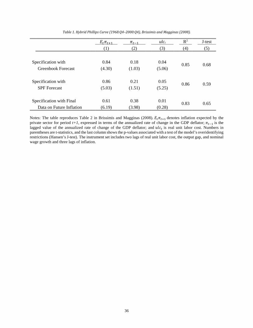
36

Table 1. Hybrid Phillips Curve (1968:Q4–2000:Q4), Brissimis and Magginas (2008).

𝐸𝐸𝑡𝑡𝜋𝜋𝑡𝑡+1 𝜋𝜋𝑡𝑡−1 ulct R2 J-test

(1) (2) (3) (4) (5)

Specification with 0.84 0.18 0.04 0.85 0.68 Greenbook Forecast (4.30) (1.03) (5.06) Specification with 0.86 0.21 0.05 0.86 0.59 SPF Forecast (5.03) (1.51) (5.25) Specification with Final 0.61 0.38 0.01 0.83 0.65 Data on Future Inflation (6.19) (3.98) (0.28)

Notes: The table reproduces Table 2 in Brissimis and Magginas (2008). 𝐸𝐸𝑡𝑡𝜋𝜋𝑡𝑡+1 denotes inflation expected by the private sector for period t+1, expressed in terms of the annualized rate of change in the GDP deflator; 𝜋𝜋𝑡𝑡−1 is the lagged value of the annualized rate of change of the GDP deflator; and 𝑢𝑢𝑢𝑢𝑜𝑜𝑡𝑡 is real unit labor cost. Numbers in parentheses are t-statistics, and the last column shows the p-values associated with a test of the model’s overidentifying restrictions (Hansen’s J-test). The instrument set includes two lags of real unit labor cost, the output gap, and nominal wage growth and three lags of inflation.

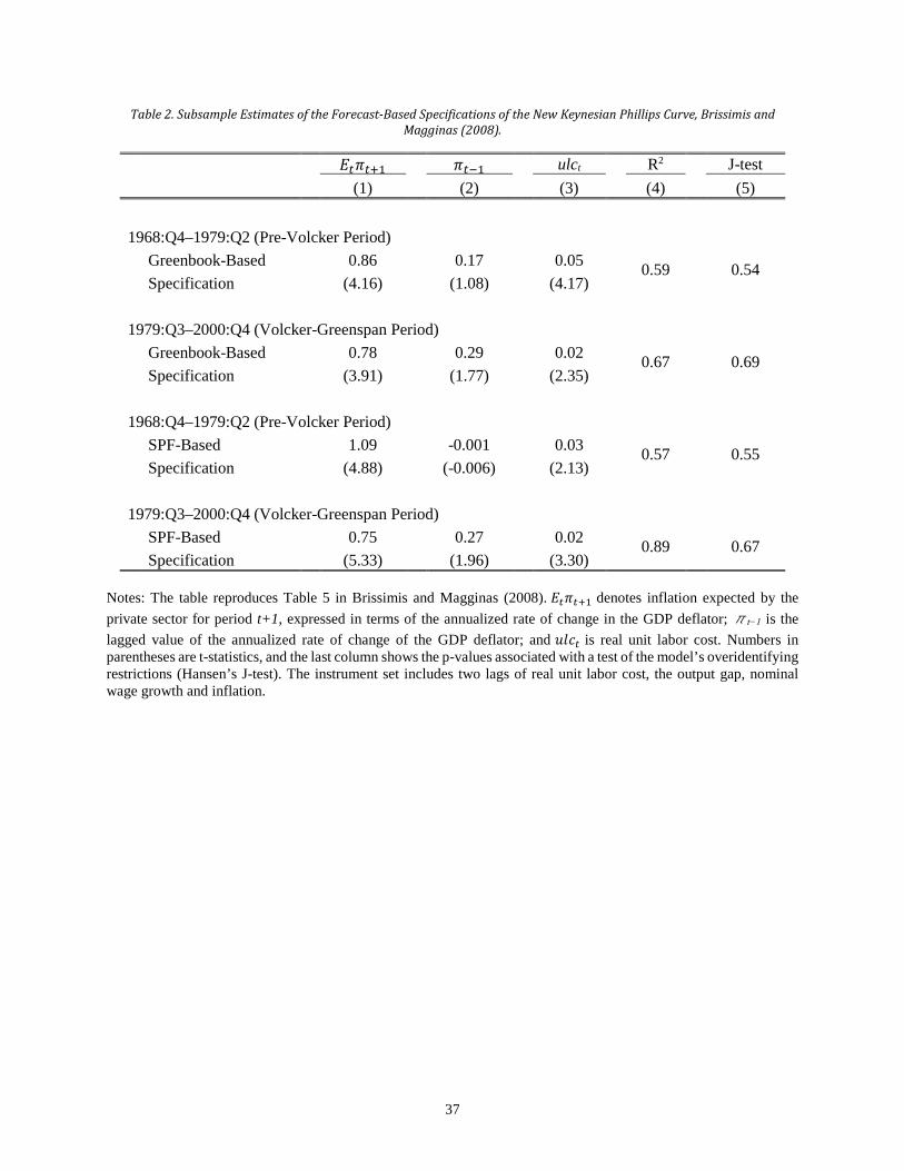
37

Table 2. Subsample Estimates of the Forecast-Based Specifications of the New Keynesian Phillips Curve, Brissimis and Magginas (2008).

𝐸𝐸𝑡𝑡𝜋𝜋𝑡𝑡+1 𝜋𝜋𝑡𝑡−1 ulct R2 J-test

(1) (2) (3) (4) (5)

1968:Q4–1979:Q2 (Pre-Volcker Period)

Greenbook-Based 0.86 0.17 0.05 0.59 0.54 Specification (4.16) (1.08) (4.17) 1979:Q3–2000:Q4 (Volcker-Greenspan Period)

Greenbook-Based 0.78 0.29 0.02 0.67 0.69 Specification (3.91) (1.77) (2.35)

1968:Q4–1979:Q2 (Pre-Volcker Period)

SPF-Based 1.09 -0.001 0.03 0.57 0.55 Specification (4.88) (-0.006) (2.13) 1979:Q3–2000:Q4 (Volcker-Greenspan Period)

SPF-Based 0.75 0.27 0.02 0.89 0.67 Specification (5.33) (1.96) (3.30)

Notes: The table reproduces Table 5 in Brissimis and Magginas (2008). 𝐸𝐸𝑡𝑡𝜋𝜋𝑡𝑡+1 denotes inflation expected by the private sector for period t+1, expressed in terms of the annualized rate of change in the GDP deflator; πt−1 is the lagged value of the annualized rate of change of the GDP deflator; and 𝑢𝑢𝑢𝑢𝑜𝑜𝑡𝑡 is real unit labor cost. Numbers in parentheses are t-statistics, and the last column shows the p-values associated with a test of the model’s overidentifying restrictions (Hansen’s J-test). The instrument set includes two lags of real unit labor cost, the output gap, nominal wage growth and inflation.

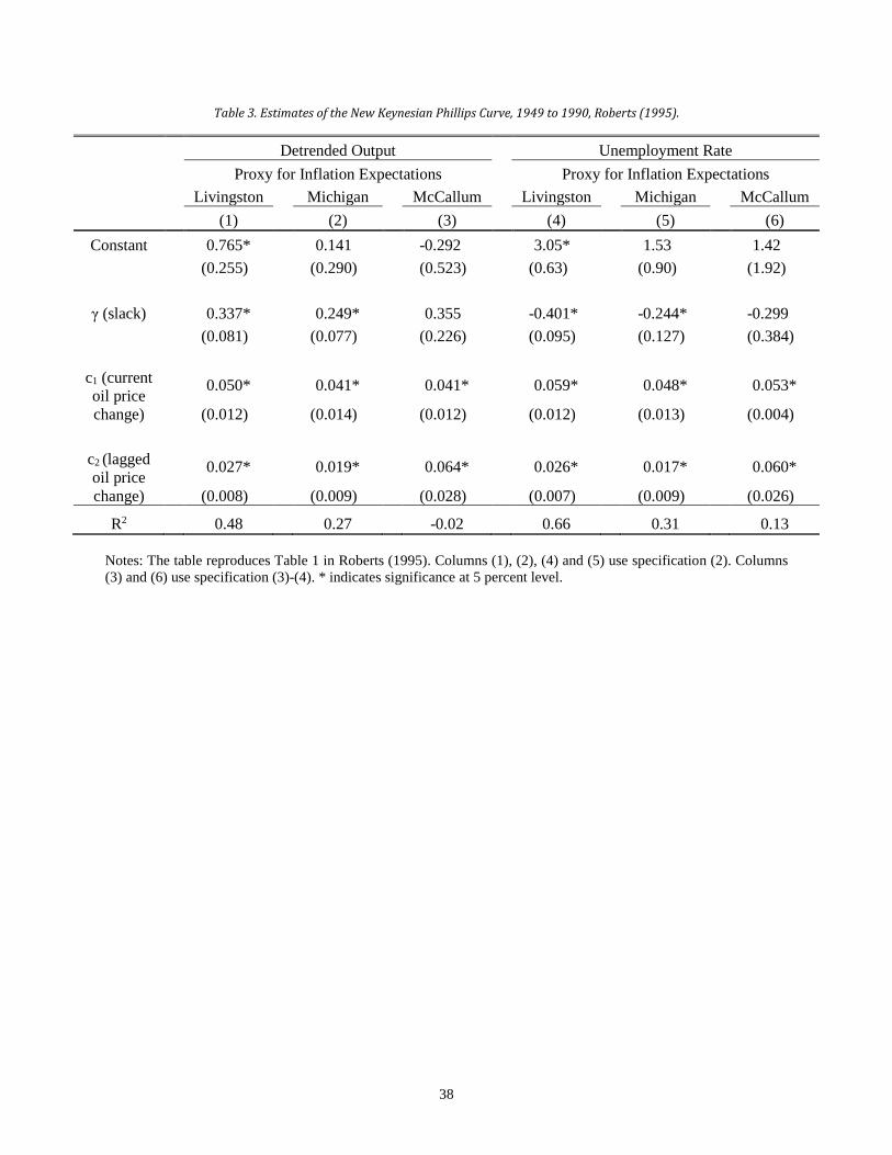
38

Table 3. Estimates of the New Keynesian Phillips Curve, 1949 to 1990, Roberts (1995).

Detrended Output Unemployment Rate

Proxy for Inflation Expectations Proxy for Inflation Expectations Livingston Michigan McCallum Livingston Michigan McCallum

(1) (2) (3) (4) (5) (6) Constant 0.765* 0.141 -0.292 3.05* 1.53 1.42

(0.255) (0.290) (0.523) (0.63) (0.90) (1.92)

γ (slack) 0.337* 0.249* 0.355 -0.401* -0.244* -0.299

(0.081) (0.077) (0.226) (0.095) (0.127) (0.384)

c1 (current oil price change)

0.050* 0.041* 0.041* 0.059* 0.048* 0.053*

(0.012) (0.014) (0.012) (0.012) (0.013) (0.004)

c2 (lagged oil price change)

0.027* 0.019* 0.064* 0.026* 0.017* 0.060*

(0.008) (0.009) (0.028) (0.007) (0.009) (0.026)

R2 0.48 0.27 -0.02 0.66 0.31 0.13 Notes: The table reproduces Table 1 in Roberts (1995). Columns (1), (2), (4) and (5) use specification (2). Columns (3) and (6) use specification (3)-(4). * indicates significance at 5 percent level.

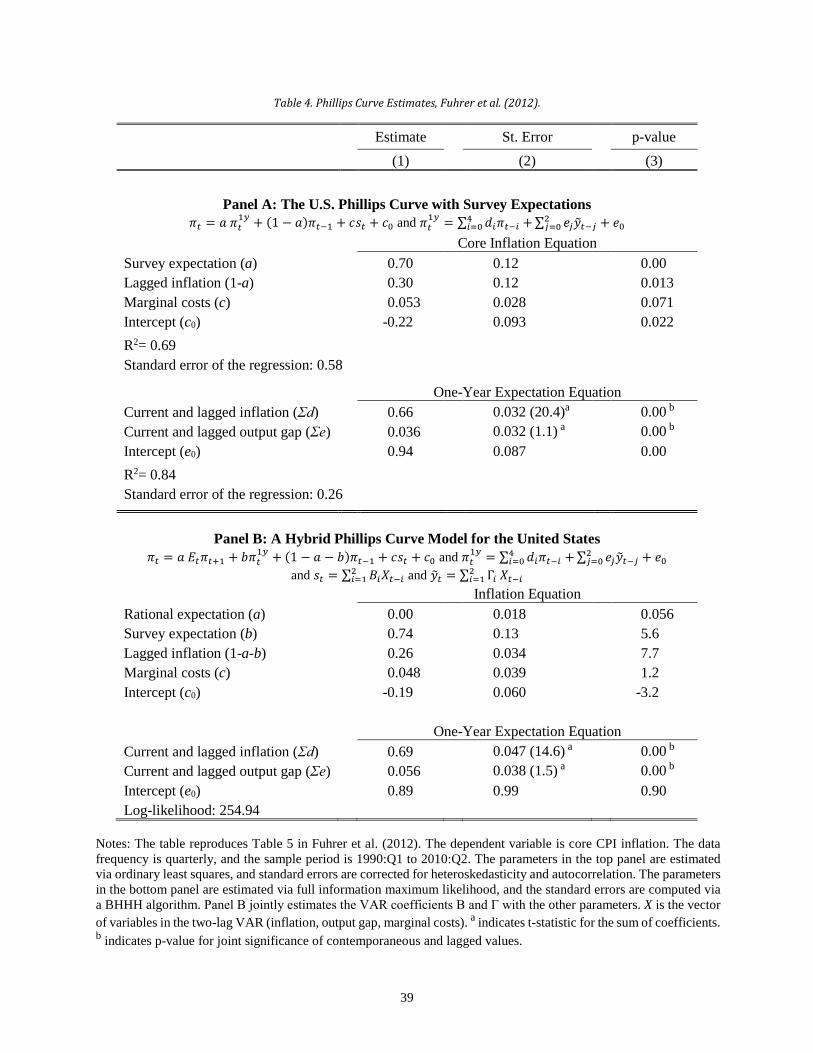
39

Table 4. Phillips Curve Estimates, Fuhrer et al. (2012).

Estimate St. Error p-value (1) (2) (3)

Panel A: The U.S. Phillips Curve with Survey Expectations 𝜋𝜋𝑡𝑡 = 𝑎𝑎 𝜋𝜋𝑡𝑡

1𝑦𝑦 + (1 − 𝑎𝑎)𝜋𝜋𝑡𝑡−1 + 𝑜𝑜𝑠𝑠𝑡𝑡 + 𝑜𝑜0 and 𝜋𝜋𝑡𝑡1𝑦𝑦 = ∑ 𝑑𝑑𝑖𝑖𝜋𝜋𝑡𝑡−𝑖𝑖 +4

𝑖𝑖=0 ∑ 𝑒𝑒𝑗𝑗𝑦𝑦�𝑡𝑡−𝑗𝑗2𝑗𝑗=0 + 𝑒𝑒0

Core Inflation Equation Survey expectation (a) 0.70 0.12 0.00 Lagged inflation (1-a) 0.30 0.12 0.013 Marginal costs (c) 0.053 0.028 0.071 Intercept (c0) -0.22 0.093 0.022 R2= 0.69 Standard error of the regression: 0.58

One-Year Expectation Equation Current and lagged inflation (Σd) 0.66 0.032 (20.4)a 0.00 b Current and lagged output gap (Σe) 0.036 0.032 (1.1) a 0.00 b Intercept (e0) 0.94 0.087 0.00 R2= 0.84 Standard error of the regression: 0.26

Panel B: A Hybrid Phillips Curve Model for the United States 𝜋𝜋𝑡𝑡 = 𝑎𝑎 𝐸𝐸𝑡𝑡𝜋𝜋𝑡𝑡+1 + 𝑏𝑏𝜋𝜋𝑡𝑡

1𝑦𝑦 + (1 − 𝑎𝑎 − 𝑏𝑏)𝜋𝜋𝑡𝑡−1 + 𝑜𝑜𝑠𝑠𝑡𝑡 + 𝑜𝑜0 and 𝜋𝜋𝑡𝑡1𝑦𝑦 = ∑ 𝑑𝑑𝑖𝑖𝜋𝜋𝑡𝑡−𝑖𝑖 +4

𝑖𝑖=0 ∑ 𝑒𝑒𝑗𝑗𝑦𝑦�𝑡𝑡−𝑗𝑗2𝑗𝑗=0 + 𝑒𝑒0

and 𝑠𝑠𝑡𝑡 = ∑ 𝐵𝐵𝑖𝑖𝑋𝑋𝑡𝑡−𝑖𝑖2𝑖𝑖=1 and 𝑦𝑦�𝑡𝑡 = ∑ Γ𝑖𝑖 𝑋𝑋𝑡𝑡−𝑖𝑖2

𝑖𝑖=1 Inflation Equation Rational expectation (a) 0.00 0.018 0.056 Survey expectation (b) 0.74 0.13 5.6 Lagged inflation (1-a-b) 0.26 0.034 7.7 Marginal costs (c) 0.048 0.039 1.2 Intercept (c0) -0.19 0.060 -3.2

One-Year Expectation Equation

Current and lagged inflation (Σd) 0.69 0.047 (14.6) a 0.00 b Current and lagged output gap (Σe) 0.056 0.038 (1.5) a 0.00 b Intercept (e0) 0.89 0.99 0.90 Log-likelihood: 254.94

Notes: The table reproduces Table 5 in Fuhrer et al. (2012). The dependent variable is core CPI inflation. The data frequency is quarterly, and the sample period is 1990:Q1 to 2010:Q2. The parameters in the top panel are estimated via ordinary least squares, and standard errors are corrected for heteroskedasticity and autocorrelation. The parameters in the bottom panel are estimated via full information maximum likelihood, and the standard errors are computed via a BHHH algorithm. Panel B jointly estimates the VAR coefficients B and Γ with the other parameters. X is the vector of variables in the two-lag VAR (inflation, output gap, marginal costs). a indicates t-statistic for the sum of coefficients. b indicates p-value for joint significance of contemporaneous and lagged values.

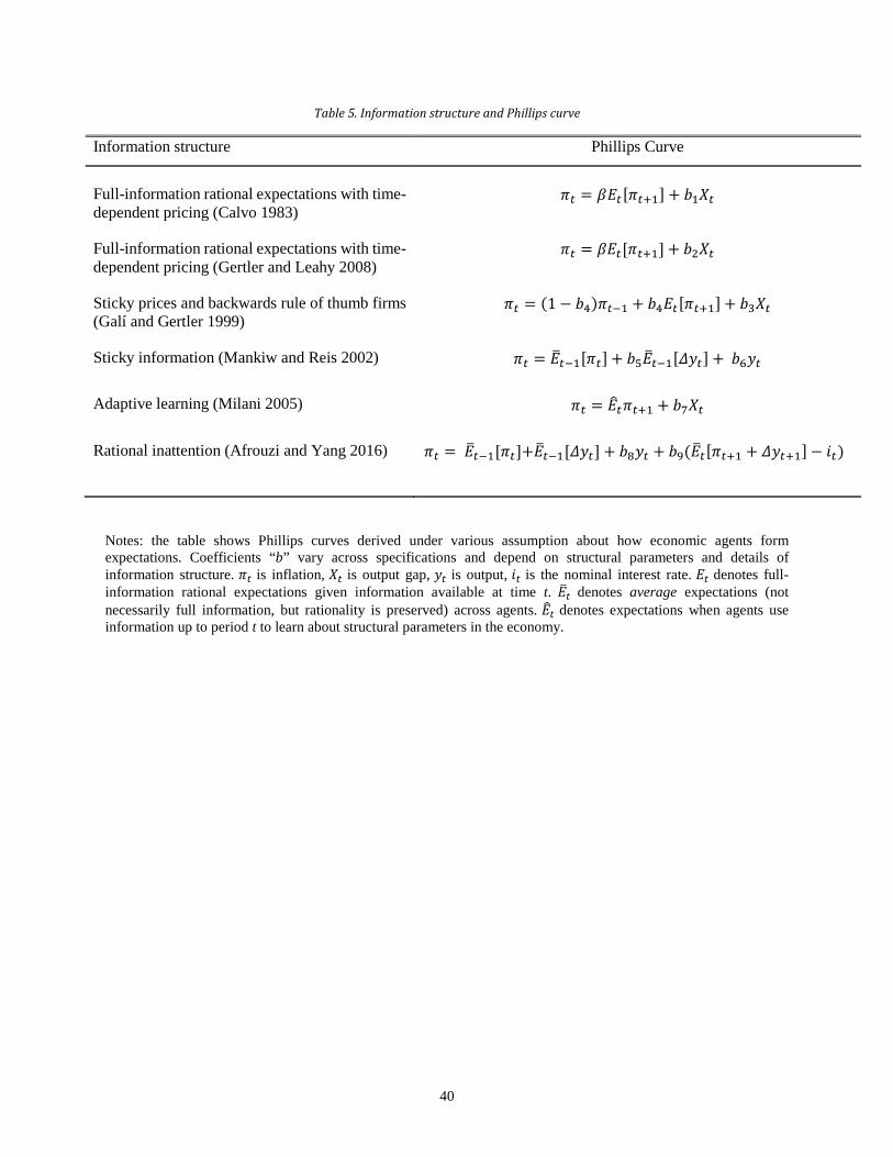
40

Table 5. Information structure and Phillips curve

Information structure Phillips Curve

Full-information rational expectations with time-dependent pricing (Calvo 1983)

𝜋𝜋𝑡𝑡 = 𝛽𝛽𝐸𝐸𝑡𝑡[𝜋𝜋𝑡𝑡+1] + 𝑏𝑏1𝑋𝑋𝑡𝑡

Full-information rational expectations with time-dependent pricing (Gertler and Leahy 2008)

𝜋𝜋𝑡𝑡 = 𝛽𝛽𝐸𝐸𝑡𝑡[𝜋𝜋𝑡𝑡+1] + 𝑏𝑏2𝑋𝑋𝑡𝑡

Sticky prices and backwards rule of thumb firms (Galí and Gertler 1999)

𝜋𝜋𝑡𝑡 = (1 − 𝑏𝑏4)𝜋𝜋𝑡𝑡−1 + 𝑏𝑏4𝐸𝐸𝑡𝑡[𝜋𝜋𝑡𝑡+1] + 𝑏𝑏3𝑋𝑋𝑡𝑡

Sticky information (Mankiw and Reis 2002) 𝜋𝜋𝑡𝑡 = 𝐸𝐸�𝑡𝑡−1[𝜋𝜋𝑡𝑡] + 𝑏𝑏5𝐸𝐸�𝑡𝑡−1[𝛥𝛥𝑦𝑦𝑡𝑡] + 𝑏𝑏6𝑦𝑦𝑡𝑡

Adaptive learning (Milani 2005) 𝜋𝜋𝑡𝑡 = 𝐸𝐸�𝑡𝑡𝜋𝜋𝑡𝑡+1 + 𝑏𝑏7𝑋𝑋𝑡𝑡

Rational inattention (Afrouzi and Yang 2016)

𝜋𝜋𝑡𝑡 = 𝐸𝐸�𝑡𝑡−1[𝜋𝜋𝑡𝑡]+𝐸𝐸�𝑡𝑡−1[𝛥𝛥𝑦𝑦𝑡𝑡] + 𝑏𝑏8𝑦𝑦𝑡𝑡 + 𝑏𝑏9(𝐸𝐸�𝑡𝑡[𝜋𝜋𝑡𝑡+1 + 𝛥𝛥𝑦𝑦𝑡𝑡+1]− 𝑟𝑟𝑡𝑡)

Notes: the table shows Phillips curves derived under various assumption about how economic agents form expectations. Coefficients “b” vary across specifications and depend on structural parameters and details of information structure. 𝜋𝜋𝑡𝑡 is inflation, 𝑋𝑋𝑡𝑡 is output gap, 𝑦𝑦𝑡𝑡 is output, 𝑟𝑟𝑡𝑡 is the nominal interest rate. 𝐸𝐸𝑡𝑡 denotes full-information rational expectations given information available at time t. 𝐸𝐸�𝑡𝑡 denotes average expectations (not necessarily full information, but rationality is preserved) across agents. 𝐸𝐸�𝑡𝑡 denotes expectations when agents use information up to period t to learn about structural parameters in the economy.

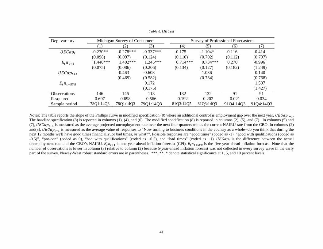
41

Table 6. LIE Test

Dep. var.: 𝜋𝜋𝑡𝑡 Michigan Survey of Consumers Survey of Professional Forecasters (1) (2) (3) (4) (5) (6) (7)

𝑈𝑈𝐸𝐸𝑈𝑈𝑎𝑎𝑝𝑝𝑡𝑡 -0.230** -0.278*** -0.337*** -0.175 -1.104* -0.116 -0.414 (0.098) (0.097) (0.124) (0.110) (0.702) (0.112) (0.797)

𝐸𝐸𝑡𝑡𝜋𝜋𝑡𝑡+1 1.440*** 1.402*** 1.245*** 0.714*** 0.734*** 0.270 -0.996 (0.075) (0.086) (0.206) (0.134) (0.127) (0.182) (1.249)

𝑈𝑈𝐸𝐸𝑈𝑈𝑎𝑎𝑝𝑝𝑡𝑡+1 -0.463 -0.608 1.036 0.140 (0.469) (0.582) (0.734) (0.768)

𝐸𝐸𝑡𝑡𝜋𝜋𝑡𝑡+5𝑌𝑌𝑌𝑌 0.172 1.507 (0.175) (1.427) Observations 146 146 118 132 132 91 91 R-squared 0.697 0.698 0.566 0.192 0.202 0.021 0.034 Sample period 78Q1:14Q3 78Q1:14Q3 79Q1:14Q3 81Q3:14Q5 81Q3:14Q3 91Q4:14Q3 91Q4:14Q3

Notes: The table reports the slope of the Phillips curve in modified specification (8) where an additional control is employment gap over the next year, 𝑈𝑈𝐸𝐸𝑈𝑈𝑎𝑎𝑝𝑝𝑡𝑡+1. The baseline specification (8) is reported in columns (1), (4), and (6). The modified specification (8) is reported in columns (2), (5), and (7). In columns (5) and (7), 𝑈𝑈𝐸𝐸𝑈𝑈𝑎𝑎𝑝𝑝𝑡𝑡+1 is measured as the average projected unemployment rate over the next four quarters minus the current NAIRU rate from the CBO. In columns (2) and(3), 𝑈𝑈𝐸𝐸𝑈𝑈𝑎𝑎𝑝𝑝𝑡𝑡+1 is measured as the average value of responses to “Now turning to business conditions in the country as a whole--do you think that during the next 12 months we'll have good times financially, or bad times, or what?”. Possible responses are “good times” (coded as -1), “good with qualifications (coded as -0.5)”, “pro-con” (coded as 0), “bad with qualifications” (coded as +0.5), and “bad times” (coded as +1). 𝑈𝑈𝐸𝐸𝑈𝑈𝑎𝑎𝑝𝑝𝑡𝑡 is the difference between the actual unemployment rate and the CBO’s NAIRU. 𝐸𝐸𝑡𝑡𝜋𝜋𝑡𝑡+1 is one-year-ahead inflation forecast (CPI). 𝐸𝐸𝑡𝑡𝜋𝜋𝑡𝑡+5𝑌𝑌𝑌𝑌 is the five year ahead inflation forecast. Note that the number of observations is lower in column (3) relative to column (2) because 5-year-ahead inflation forecast was not collected in every survey wave in the early part of the survey. Newey-West robust standard errors are in parentheses. ***, **, * denote statistical significance at 1, 5, and 10 percent levels.

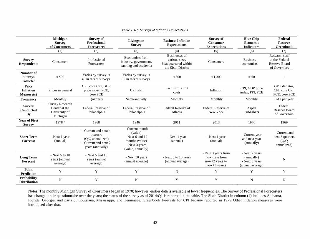
42

Table 7. U.S. Surveys of Inflation Expectations.

Michigan

Survey of Consumers

Survey of Professional Forecasters

Livingston Survey

Business Inflation Expectations

Survey of Consumer

Expectations

Blue Chip Economic Indicators

Federal Reserve

Greenbook (1) (2) (3) (4) (5) (6) (7)

Survey Respondents

Consumers Professional Forecasters

Economists from

industry, government, banking and academia

Businesses of various sizes

headquartered within the Sixth District

Consumers Business economists

Research staff at the Federal Reserve Board of Governors

Number of Surveys

Collected

≈ 500 Varies by survey. ≈

40 in recent surveys. Varies by survey. ≈ 30 in recent surveys.

≈ 300 ≈ 1,300 ≈ 50 1

Price Inflation

Measure(s)

Prices in general

CPI, core CPI, GDP price index, PCE,

core PCE CPI, PPI Each firm’s unit

costs Inflation CPI, GDP price

index, PPI, PCE

GDP deflator, CPI, core CPI, PCE, core PCE

Frequency Monthly Quarterly Semi-annually Monthly Monthly Monthly 8-12 per year

Survey Conducted

By

Survey Research Center at the University of

Michigan

Federal Reserve of Philadelphia

Federal Reserve of Philadelphia

Federal Reserve of Atlanta

Federal Reserve of New York

Aspen Publishers

Federal

Reserve Board of Governors

Year of First Survey

1978 1 1968 1946 2011 2013 1976 1969

Short Term Forecast

- Next 1 year (annual)

- Current and next 4 quarters

(Q/Q annualized) - Current and next 2

years (annually)

- Current month (value)

- Next 6 and 12 months (value) - Next 3 years

(value, annually)

- Next 1 year (annual)

- Next 1 year (annual)

- Current year and next year

(annually)

- Current and next 8 quarters

(Q/Q annualized)

Long Term Forecast

- Next 5 to 10 years (annual

average)

- Next 5 and 10 years (annual

average) - Next 10 years

(annual average) - Next 5 to 10 years

(annual average)

- Rate 3 years from now (rate from now+2 years to now+3 years)

- Next 7 years

(annually) - Next 5 years

(annual average)

N

Point Prediction

Y Y Y N Y Y Y

Probability Distribution

N Y N Y Y N N

Notes: The monthly Michigan Survey of Consumers began in 1978; however, earlier data is available at lower frequencies. The Survey of Professional Forecasters has changed their questionnaire over the years; the status of the survey as of 2014:Q1 is reported in the table. The Sixth District in column (4) includes Alabama, Florida, Georgia, and parts of Louisiana, Mississippi, and Tennessee. Greenbook forecasts for CPI became reported in 1979 Other inflation measures were introduced after that.

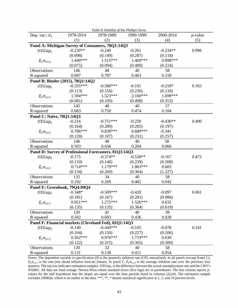
43

Table 8. Stability of the Phillips Curve. Dep. var.: 𝜋𝜋𝑡𝑡 1978-2014 1978-1989 1990-1999 2000-2014 p-value

(1) (2) (3) (4) (5) Panel A: Michigan Survey of Consumers, 78Q1:14Q3

𝑈𝑈𝐸𝐸𝑈𝑈𝑎𝑎𝑝𝑝𝑡𝑡 -0.230** -0.240 -0.261 -0.234** 0.996 (0.098) (0.149) (0.287) (0.118)

𝐸𝐸𝑡𝑡𝜋𝜋𝑡𝑡+1 1.440*** 1.515*** 1.469*** 0.898*** (0.075) (0.094) (0.400) (0.224) Observations 146 48 40 58 R-squared 0.697 0.787 0.463 0.159 Panel B: Binder (2015), 78Q1:14Q2

𝑈𝑈𝐸𝐸𝑈𝑈𝑎𝑎𝑝𝑝𝑡𝑡 -0.335*** -0.580*** -0.191 -0.218* 0.163 (0.113) (0.156) (0.230) (0.118)

𝐸𝐸𝑡𝑡𝜋𝜋𝑡𝑡+1 1.594*** 1.523*** 2.160*** 1.699*** (0.081) (0.109) (0.498) (0.353) Observations 145 48 40 57 R-squared 0.683 0.750 0.474 0.184 Panel C: Naïve, 78Q1:14Q3

𝑈𝑈𝐸𝐸𝑈𝑈𝑎𝑎𝑝𝑝𝑡𝑡 -0.216 -0.751*** -0.250 -0.436** 0.490 (0.164) (0.289) (0.265) (0.197)

𝐸𝐸𝑡𝑡𝜋𝜋𝑡𝑡+1 0.786*** 0.838*** 0.689*** -0.341 (0.120) (0.107) (0.231) (0.257) Observations 146 48 40 58 R-squared 0.503 0.636 0.264 0.066 Panel D: Survey of Professional Forecasters, 81Q3:14Q3

𝑈𝑈𝐸𝐸𝑈𝑈𝑎𝑎𝑝𝑝𝑡𝑡 -0.175 -0.374** -0.538** -0.167 0.472 (0.110) (0.146) (0.239) (0.208)

𝐸𝐸𝑡𝑡𝜋𝜋𝑡𝑡+1 0.714*** 1.179*** 1.863*** 0.603 (0.134) (0.269) (0.364) (1.227) Observations 132 34 40 58 R-squared 0.192 0.269 0.482 0.042 Panel E: Greenbook, 79Q4:09Q4

𝑈𝑈𝐸𝐸𝑈𝑈𝑎𝑎𝑝𝑝𝑡𝑡 -0.348* -0.509*** -0.420 -0.097 0.061 (0.181) (0.167) (0.281) (0.086)

𝐸𝐸𝑡𝑡𝜋𝜋𝑡𝑡+1 0.951*** 1.275*** 1.526*** 0.632 (0.135) (0.135) (0.364) (0.619) Observations 120 41 40 39 R-squared 0.502 0.683 0.436 0.028 Panel F: Financial markets (Cleveland Fed), 82Q1:14Q3

𝑈𝑈𝐸𝐸𝑈𝑈𝑎𝑎𝑝𝑝𝑡𝑡 -0.140 -0.449*** -0.105 -0.078 0.241 (0.104) (0.150) (0.227) (0.206)

𝐸𝐸𝑡𝑡𝜋𝜋𝑡𝑡+1 0.562*** 0.976*** 1.719*** 0.630 (0.122) (0.315) (0.365) (0.500) Observations 130 32 40 58 R-squared 0.131 0.138 0.411 0.054

Notes: The dependent variable in specification (9) is the quarterly inflation rate (CPI, annualized). In all panels (except Panel C), 𝐸𝐸𝑡𝑡𝜋𝜋𝑡𝑡+1 is the one-year ahead inflation forecast (mean). In panel C, 𝐸𝐸𝑡𝑡𝜋𝜋𝑡𝑡+1 is the average inflation rate over the previous four quarters. The top row indicates estimation samples. 𝑈𝑈𝐸𝐸𝑈𝑈𝑎𝑎𝑝𝑝𝑡𝑡 is the difference between the actual unemployment rate and the CBO’s NAIRU. All data are final-vintage. Newey-West robust standard errors (five lags) are in parentheses. The last column reports p-values for the null hypothesis that the slopes are equal over the time periods listed in columns (2)-(4). The estimation sample excludes 2008Q4, which is an outlier in the data. ***, **, * denote statistical significance at 1, 5, and 10 percent levels.

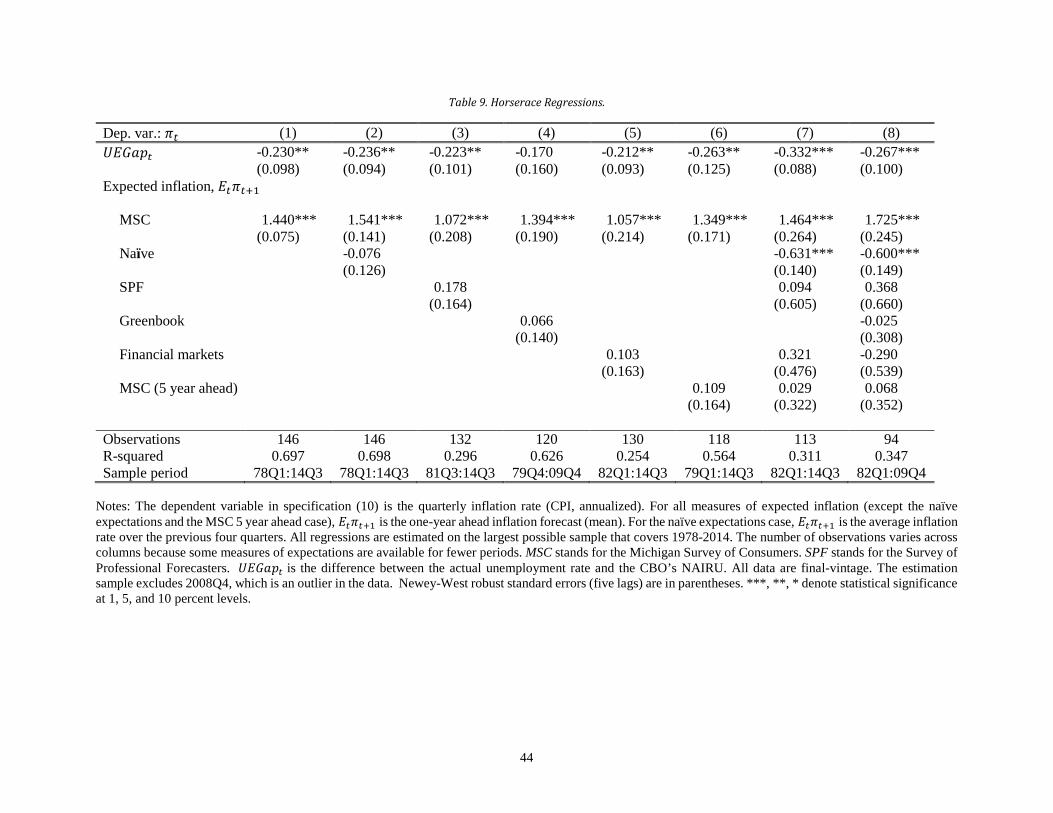
44

Table 9. Horserace Regressions.

Dep. var.: 𝜋𝜋𝑡𝑡 (1) (2) (3) (4) (5) (6) (7) (8) 𝑈𝑈𝐸𝐸𝑈𝑈𝑎𝑎𝑝𝑝𝑡𝑡 -0.230** -0.236** -0.223** -0.170 -0.212** -0.263** -0.332*** -0.267*** (0.098) (0.094) (0.101) (0.160) (0.093) (0.125) (0.088) (0.100) Expected inflation, 𝐸𝐸𝑡𝑡𝜋𝜋𝑡𝑡+1

MSC 1.440*** 1.541*** 1.072*** 1.394*** 1.057*** 1.349*** 1.464*** 1.725*** (0.075) (0.141) (0.208) (0.190) (0.214) (0.171) (0.264) (0.245) Naïve -0.076 -0.631*** -0.600*** (0.126) (0.140) (0.149) SPF 0.178 0.094 0.368 (0.164) (0.605) (0.660) Greenbook 0.066 -0.025 (0.140) (0.308) Financial markets 0.103 0.321 -0.290 (0.163) (0.476) (0.539) MSC (5 year ahead) 0.109 0.029 0.068

(0.164) (0.322) (0.352) Observations 146 146 132 120 130 118 113 94 R-squared 0.697 0.698 0.296 0.626 0.254 0.564 0.311 0.347 Sample period 78Q1:14Q3 78Q1:14Q3 81Q3:14Q3 79Q4:09Q4 82Q1:14Q3 79Q1:14Q3 82Q1:14Q3 82Q1:09Q4

Notes: The dependent variable in specification (10) is the quarterly inflation rate (CPI, annualized). For all measures of expected inflation (except the naïve expectations and the MSC 5 year ahead case), 𝐸𝐸𝑡𝑡𝜋𝜋𝑡𝑡+1 is the one-year ahead inflation forecast (mean). For the naïve expectations case, 𝐸𝐸𝑡𝑡𝜋𝜋𝑡𝑡+1 is the average inflation rate over the previous four quarters. All regressions are estimated on the largest possible sample that covers 1978-2014. The number of observations varies across columns because some measures of expectations are available for fewer periods. MSC stands for the Michigan Survey of Consumers. SPF stands for the Survey of Professional Forecasters. 𝑈𝑈𝐸𝐸𝑈𝑈𝑎𝑎𝑝𝑝𝑡𝑡 is the difference between the actual unemployment rate and the CBO’s NAIRU. All data are final-vintage. The estimation sample excludes 2008Q4, which is an outlier in the data. Newey-West robust standard errors (five lags) are in parentheses. ***, **, * denote statistical significance at 1, 5, and 10 percent levels.

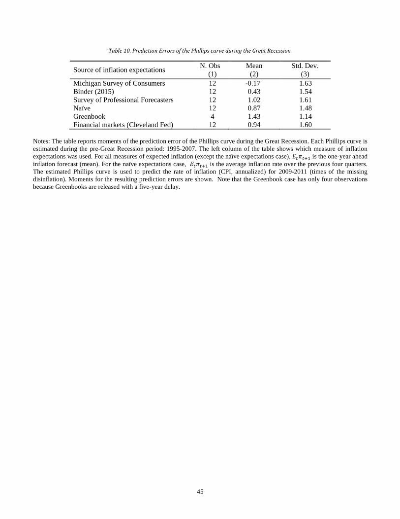
45

Table 10. Prediction Errors of the Phillips curve during the Great Recession.

Source of inflation expectations N. Obs Mean Std. Dev. (1) (2) (3)

Michigan Survey of Consumers 12 -0.17 1.63 Binder (2015) 12 0.43 1.54 Survey of Professional Forecasters 12 1.02 1.61 Naïve 12 0.87 1.48 Greenbook 4 1.43 1.14 Financial markets (Cleveland Fed) 12 0.94 1.60

Notes: The table reports moments of the prediction error of the Phillips curve during the Great Recession. Each Phillips curve is estimated during the pre-Great Recession period: 1995-2007. The left column of the table shows which measure of inflation expectations was used. For all measures of expected inflation (except the naïve expectations case), 𝐸𝐸𝑡𝑡𝜋𝜋𝑡𝑡+1 is the one-year ahead inflation forecast (mean). For the naïve expectations case, 𝐸𝐸𝑡𝑡𝜋𝜋𝑡𝑡+1 is the average inflation rate over the previous four quarters. The estimated Phillips curve is used to predict the rate of inflation (CPI, annualized) for 2009-2011 (times of the missing disinflation). Moments for the resulting prediction errors are shown. Note that the Greenbook case has only four observations because Greenbooks are released with a five-year delay.

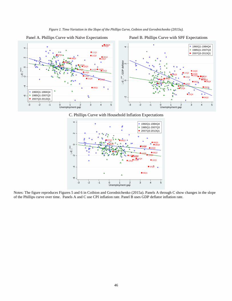
46

Figure 1. Time Variation in the Slope of the Phillips Curve, Coibion and Gorodnichenko (2015a).

Panel A. Phillips Curve with Naïve Expectations Panel B. Phillips Curve with SPF Expectations

C. Phillips Curve with Household Inflation Expectations

Notes: The figure reproduces Figures 5 and 6 in Coibion and Gorodnichenko (2015a). Panels A through C show changes in the slope of the Phillips curve over time. Panels A and C use CPI inflation rate. Panel B uses GDP deflator inflation rate.

07Q4

08Q1

08Q2

08Q3

09Q1

09Q2

09Q309Q4

10Q1

10Q2

10Q3

10Q4

11Q111Q2

11Q3

11Q4

12Q1

12Q2

12Q312Q4

13Q1

-6-4

-20

24

t-E t

BAC

K

-3 -2 -1 0 1 2 3 4 5Unemployment gap

1960Q1-1984Q41985Q1-2007Q32007Q3-2013Q1

07Q4

08Q108Q2

08Q3

09Q1

09Q2

09Q3

09Q410Q110Q2

10Q310Q411Q111Q211Q3

11Q4

12Q1

12Q2

12Q3

12Q413Q1

-20

24

t-E t

SPF , G

DP

defla

tor

-3 -2 -1 0 1 2 3 4 5Unemployment gap

1960Q1-1984Q41985Q1-2007Q32007Q3-2013Q1

07Q4

08Q1

08Q2

08Q3

09Q1

09Q2

09Q309Q4

10Q1

10Q2

10Q3

10Q411Q111Q2

11Q3

11Q412Q1

12Q212Q312Q4

13Q1

-6-4

-20

24

t-E t

MSC

-3 -2 -1 0 1 2 3 4 5Unemployment gap

1960Q1-1984Q41985Q1-2007Q32007Q3-2013Q1

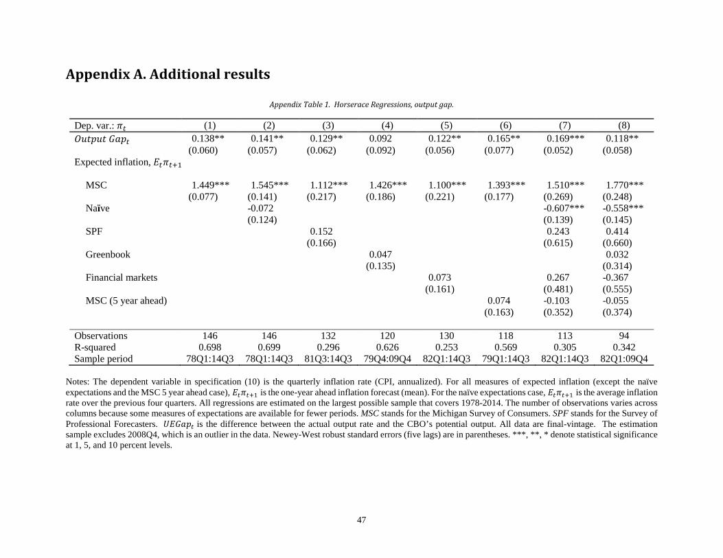
47

Appendix A. Additional results

Appendix Table 1. Horserace Regressions, output gap.

Dep. var.: 𝜋𝜋𝑡𝑡 (1) (2) (3) (4) (5) (6) (7) (8) 𝑂𝑂𝑢𝑢𝑡𝑡𝑝𝑝𝑢𝑢𝑡𝑡 𝑈𝑈𝑎𝑎𝑝𝑝𝑡𝑡 0.138** 0.141** 0.129** 0.092 0.122** 0.165** 0.169*** 0.118** (0.060) (0.057) (0.062) (0.092) (0.056) (0.077) (0.052) (0.058) Expected inflation, 𝐸𝐸𝑡𝑡𝜋𝜋𝑡𝑡+1

MSC 1.449*** 1.545*** 1.112*** 1.426*** 1.100*** 1.393*** 1.510*** 1.770*** (0.077) (0.141) (0.217) (0.186) (0.221) (0.177) (0.269) (0.248) Naïve -0.072 -0.607*** -0.558*** (0.124) (0.139) (0.145) SPF 0.152 0.243 0.414 (0.166) (0.615) (0.660) Greenbook 0.047 0.032 (0.135) (0.314) Financial markets 0.073 0.267 -0.367 (0.161) (0.481) (0.555) MSC (5 year ahead) 0.074 -0.103 -0.055

(0.163) (0.352) (0.374) Observations 146 146 132 120 130 118 113 94 R-squared 0.698 0.699 0.296 0.626 0.253 0.569 0.305 0.342 Sample period 78Q1:14Q3 78Q1:14Q3 81Q3:14Q3 79Q4:09Q4 82Q1:14Q3 79Q1:14Q3 82Q1:14Q3 82Q1:09Q4

Notes: The dependent variable in specification (10) is the quarterly inflation rate (CPI, annualized). For all measures of expected inflation (except the naïve expectations and the MSC 5 year ahead case), 𝐸𝐸𝑡𝑡𝜋𝜋𝑡𝑡+1 is the one-year ahead inflation forecast (mean). For the naïve expectations case, 𝐸𝐸𝑡𝑡𝜋𝜋𝑡𝑡+1 is the average inflation rate over the previous four quarters. All regressions are estimated on the largest possible sample that covers 1978-2014. The number of observations varies across columns because some measures of expectations are available for fewer periods. MSC stands for the Michigan Survey of Consumers. SPF stands for the Survey of Professional Forecasters. 𝑈𝑈𝐸𝐸𝑈𝑈𝑎𝑎𝑝𝑝𝑡𝑡 is the difference between the actual output rate and the CBO’s potential output. All data are final-vintage. The estimation sample excludes 2008Q4, which is an outlier in the data. Newey-West robust standard errors (five lags) are in parentheses. ***, **, * denote statistical significance at 1, 5, and 10 percent levels.

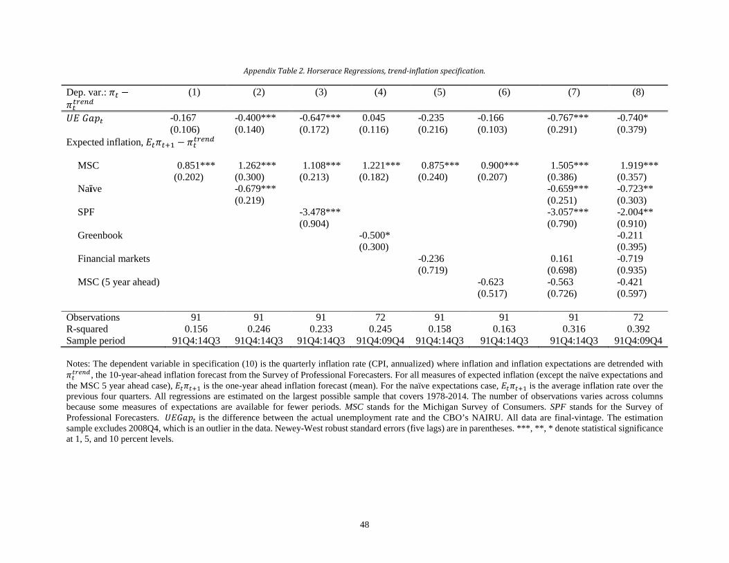
48

Appendix Table 2. Horserace Regressions, trend-inflation specification.

Dep. var.: 𝜋𝜋𝑡𝑡 −𝜋𝜋𝑡𝑡𝑡𝑡𝑡𝑡𝑡𝑡𝑛𝑛𝑡𝑡

(1) (2) (3) (4) (5) (6) (7) (8)

𝑈𝑈𝐸𝐸 𝑈𝑈𝑎𝑎𝑝𝑝𝑡𝑡 -0.167 -0.400*** -0.647*** 0.045 -0.235 -0.166 -0.767*** -0.740* (0.106) (0.140) (0.172) (0.116) (0.216) (0.103) (0.291) (0.379) Expected inflation, 𝐸𝐸𝑡𝑡𝜋𝜋𝑡𝑡+1 − 𝜋𝜋𝑡𝑡𝑡𝑡𝑡𝑡𝑡𝑡𝑛𝑛𝑡𝑡

MSC 0.851*** 1.262*** 1.108*** 1.221*** 0.875*** 0.900*** 1.505*** 1.919*** (0.202) (0.300) (0.213) (0.182) (0.240) (0.207) (0.386) (0.357) Naïve -0.679*** -0.659*** -0.723** (0.219) (0.251) (0.303) SPF -3.478*** -3.057*** -2.004** (0.904) (0.790) (0.910) Greenbook -0.500* -0.211 (0.300) (0.395) Financial markets -0.236 0.161 -0.719 (0.719) (0.698) (0.935) MSC (5 year ahead) -0.623 -0.563 -0.421

(0.517) (0.726) (0.597) Observations 91 91 91 72 91 91 91 72 R-squared 0.156 0.246 0.233 0.245 0.158 0.163 0.316 0.392 Sample period 91Q4:14Q3 91Q4:14Q3 91Q4:14Q3 91Q4:09Q4 91Q4:14Q3 91Q4:14Q3 91Q4:14Q3 91Q4:09Q4 Notes: The dependent variable in specification (10) is the quarterly inflation rate (CPI, annualized) where inflation and inflation expectations are detrended with 𝜋𝜋𝑡𝑡𝑡𝑡𝑡𝑡𝑡𝑡𝑛𝑛𝑡𝑡, the 10-year-ahead inflation forecast from the Survey of Professional Forecasters. For all measures of expected inflation (except the naïve expectations and the MSC 5 year ahead case), 𝐸𝐸𝑡𝑡𝜋𝜋𝑡𝑡+1 is the one-year ahead inflation forecast (mean). For the naïve expectations case, 𝐸𝐸𝑡𝑡𝜋𝜋𝑡𝑡+1 is the average inflation rate over the previous four quarters. All regressions are estimated on the largest possible sample that covers 1978-2014. The number of observations varies across columns because some measures of expectations are available for fewer periods. MSC stands for the Michigan Survey of Consumers. SPF stands for the Survey of Professional Forecasters. 𝑈𝑈𝐸𝐸𝑈𝑈𝑎𝑎𝑝𝑝𝑡𝑡 is the difference between the actual unemployment rate and the CBO’s NAIRU. All data are final-vintage. The estimation sample excludes 2008Q4, which is an outlier in the data. Newey-West robust standard errors (five lags) are in parentheses. ***, **, * denote statistical significance at 1, 5, and 10 percent levels.

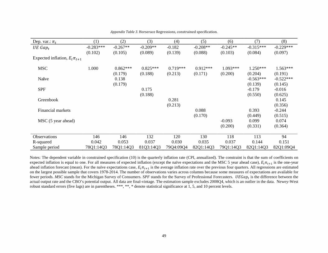
49

Appendix Table 3. Horserace Regressions, constrained specification.

Dep. var.: 𝜋𝜋𝑡𝑡 (1) (2) (3) (4) (5) (6) (7) (8) 𝑈𝑈𝐸𝐸 𝑈𝑈𝑎𝑎𝑝𝑝𝑡𝑡 -0.283*** -0.267** -0.209** -0.182 -0.208** -0.245** -0.315*** -0.229*** (0.102) (0.105) (0.089) (0.139) (0.088) (0.103) (0.084) (0.097) Expected inflation, 𝐸𝐸𝑡𝑡𝜋𝜋𝑡𝑡+1

MSC 1.000 0.862*** 0.825*** 0.719*** 0.912*** 1.093*** 1.250*** 1.563*** (0.179) (0.188) (0.213) (0.171) (0.200) (0.204) (0.191) Naïve 0.138 -0.563*** -0.522*** (0.179) (0.139) (0.145) SPF 0.175 -0.179 -0.016 (0.188) (0.550) (0.625) Greenbook 0.281 0.145 (0.213) (0.356) Financial markets 0.088 0.393 -0.244 (0.170) (0.449) (0.515) MSC (5 year ahead) -0.093 0.099 0.074

(0.200) (0.331) (0.364) Observations 146 146 132 120 130 118 113 94 R-squared 0.042 0.053 0.037 0.030 0.035 0.037 0.144 0.151 Sample period 78Q1:14Q3 78Q1:14Q3 81Q3:14Q3 79Q4:09Q4 82Q1:14Q3 79Q1:14Q3 82Q1:14Q3 82Q1:09Q4

Notes: The dependent variable in constrained specification (10) is the quarterly inflation rate (CPI, annualized). The constraint is that the sum of coefficients on expected inflation is equal to one. For all measures of expected inflation (except the naïve expectations and the MSC 5 year ahead case), 𝐸𝐸𝑡𝑡𝜋𝜋𝑡𝑡+1 is the one-year ahead inflation forecast (mean). For the naïve expectations case, 𝐸𝐸𝑡𝑡𝜋𝜋𝑡𝑡+1 is the average inflation rate over the previous four quarters. All regressions are estimated on the largest possible sample that covers 1978-2014. The number of observations varies across columns because some measures of expectations are available for fewer periods. MSC stands for the Michigan Survey of Consumers. SPF stands for the Survey of Professional Forecasters. 𝑈𝑈𝐸𝐸𝑈𝑈𝑎𝑎𝑝𝑝𝑡𝑡 is the difference between the actual output rate and the CBO’s potential output. All data are final-vintage. The estimation sample excludes 2008Q4, which is an outlier in the data. Newey-West robust standard errors (five lags) are in parentheses. ***, **, * denote statistical significance at 1, 5, and 10 percent levels.

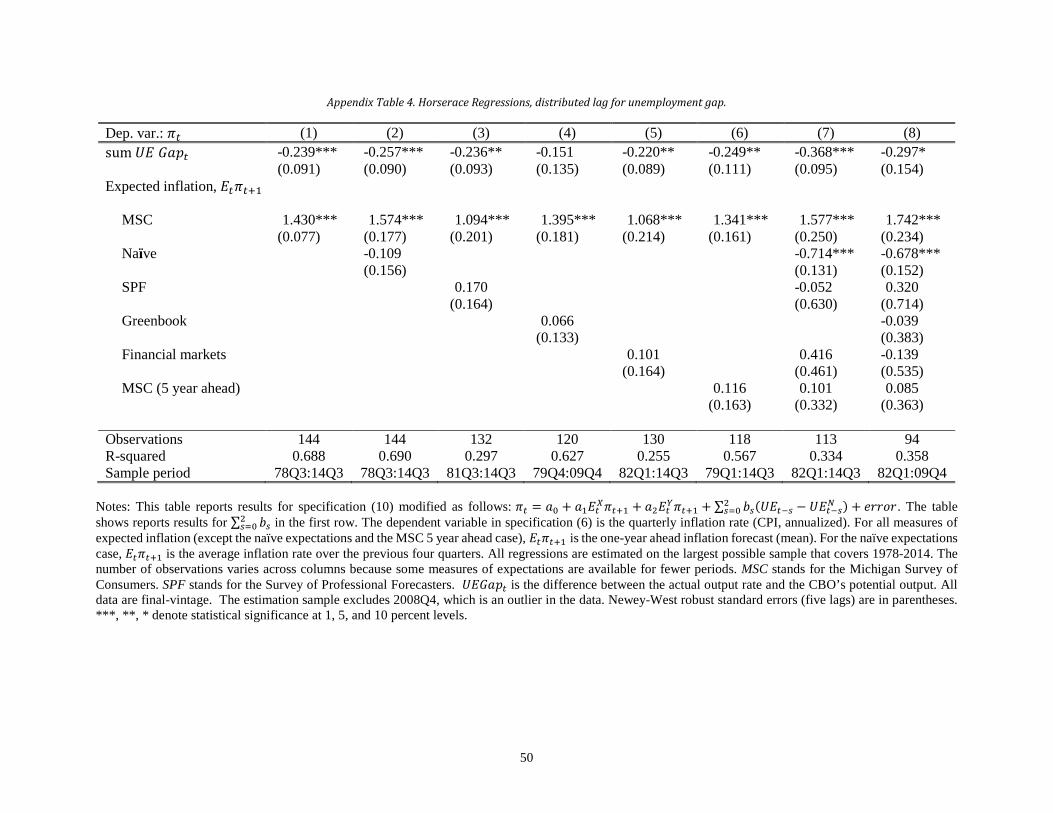
50

Appendix Table 4. Horserace Regressions, distributed lag for unemployment gap.

Dep. var.: 𝜋𝜋𝑡𝑡 (1) (2) (3) (4) (5) (6) (7) (8) sum 𝑈𝑈𝐸𝐸 𝑈𝑈𝑎𝑎𝑝𝑝𝑡𝑡 -0.239*** -0.257*** -0.236** -0.151 -0.220** -0.249** -0.368*** -0.297* (0.091) (0.090) (0.093) (0.135) (0.089) (0.111) (0.095) (0.154) Expected inflation, 𝐸𝐸𝑡𝑡𝜋𝜋𝑡𝑡+1

MSC 1.430*** 1.574*** 1.094*** 1.395*** 1.068*** 1.341*** 1.577*** 1.742*** (0.077) (0.177) (0.201) (0.181) (0.214) (0.161) (0.250) (0.234) Naïve -0.109 -0.714*** -0.678*** (0.156) (0.131) (0.152) SPF 0.170 -0.052 0.320 (0.164) (0.630) (0.714) Greenbook 0.066 -0.039 (0.133) (0.383) Financial markets 0.101 0.416 -0.139 (0.164) (0.461) (0.535) MSC (5 year ahead) 0.116 0.101 0.085

(0.163) (0.332) (0.363) Observations 144 144 132 120 130 118 113 94 R-squared 0.688 0.690 0.297 0.627 0.255 0.567 0.334 0.358 Sample period 78Q3:14Q3 78Q3:14Q3 81Q3:14Q3 79Q4:09Q4 82Q1:14Q3 79Q1:14Q3 82Q1:14Q3 82Q1:09Q4

Notes: This table reports results for specification (10) modified as follows: 𝜋𝜋𝑡𝑡 = 𝑎𝑎0 + 𝑎𝑎1𝐸𝐸𝑡𝑡𝑋𝑋𝜋𝜋𝑡𝑡+1 + 𝑎𝑎2𝐸𝐸𝑡𝑡𝑌𝑌𝜋𝜋𝑡𝑡+1 + ∑ 𝑏𝑏𝑠𝑠(𝑈𝑈𝐸𝐸𝑡𝑡−𝑠𝑠 − 𝑈𝑈𝐸𝐸𝑡𝑡−𝑠𝑠𝑁𝑁 )2

𝑠𝑠=0 + 𝑒𝑒𝑟𝑟𝑟𝑟𝑜𝑜𝑟𝑟. The table shows reports results for ∑ 𝑏𝑏𝑠𝑠2

𝑠𝑠=0 in the first row. The dependent variable in specification (6) is the quarterly inflation rate (CPI, annualized). For all measures of expected inflation (except the naïve expectations and the MSC 5 year ahead case), 𝐸𝐸𝑡𝑡𝜋𝜋𝑡𝑡+1 is the one-year ahead inflation forecast (mean). For the naïve expectations case, 𝐸𝐸𝑡𝑡𝜋𝜋𝑡𝑡+1 is the average inflation rate over the previous four quarters. All regressions are estimated on the largest possible sample that covers 1978-2014. The number of observations varies across columns because some measures of expectations are available for fewer periods. MSC stands for the Michigan Survey of Consumers. SPF stands for the Survey of Professional Forecasters. 𝑈𝑈𝐸𝐸𝑈𝑈𝑎𝑎𝑝𝑝𝑡𝑡 is the difference between the actual output rate and the CBO’s potential output. All data are final-vintage. The estimation sample excludes 2008Q4, which is an outlier in the data. Newey-West robust standard errors (five lags) are in parentheses. ***, **, * denote statistical significance at 1, 5, and 10 percent levels.

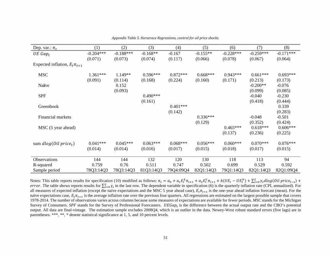
51

Appendix Table 5. Horserace Regressions, control for oil price shocks.

Dep. var.: 𝜋𝜋𝑡𝑡 (1) (2) (3) (4) (5) (6) (7) (8) 𝑈𝑈𝐸𝐸 𝑈𝑈𝑎𝑎𝑝𝑝𝑡𝑡 -0.204*** -0.188*** -0.168** -0.167 -0.155** -0.228*** -0.259*** -0.171*** (0.071) (0.073) (0.074) (0.117) (0.066) (0.078) (0.067) (0.064) Expected inflation, 𝐸𝐸𝑡𝑡𝜋𝜋𝑡𝑡+1

MSC 1.361*** 1.149** 0.596*** 0.872*** 0.668*** 0.943*** 0.661*** 0.693*** (0.091) (0.114) (0.168) (0.224) (0.160) (0.171) (0.213) (0.173) Naïve 0.152 -0.200** -0.076 (0.093) (0.099) (0.085) SPF 0.490*** -0.040 -0.230 (0.161) (0.418) (0.444) Greenbook 0.401*** 0.339 (0.142) (0.283) Financial markets 0.336*** -0.048 -0.501 (0.129) (0.352) (0.424) MSC (5 year ahead) 0.465*** 0.618*** 0.606***

(0.137) (0.236) (0.225) sum 𝑑𝑑𝑢𝑢𝑜𝑜𝑑𝑑(𝑂𝑂𝑟𝑟𝑢𝑢 𝑝𝑝𝑟𝑟𝑟𝑟𝑜𝑜𝑒𝑒𝑡𝑡) 0.041*** 0.045*** 0.063*** 0.068*** 0.056*** 0.060*** 0.070*** 0.076*** (0.014) (0.014) (0.016) (0.017) (0.015) (0.018) (0.017) (0.015) Observations 144 144 132 120 130 118 113 94 R-squared 0.759 0.76 0.511 0.747 0.502 0.699 0.529 0.592 Sample period 78Q3:14Q3 78Q3:14Q3 81Q3:14Q3 79Q4:09Q4 82Q1:14Q3 79Q1:14Q3 82Q1:14Q3 82Q1:09Q4

Notes: This table reports results for specification (10) modified as follows: 𝜋𝜋𝑡𝑡 = 𝑎𝑎0 + 𝑎𝑎1𝐸𝐸𝑡𝑡𝑋𝑋𝜋𝜋𝑡𝑡+1 + 𝑎𝑎2𝐸𝐸𝑡𝑡𝑌𝑌𝜋𝜋𝑡𝑡+1 + 𝑏𝑏(𝑈𝑈𝐸𝐸𝑡𝑡 − 𝑈𝑈𝐸𝐸𝑡𝑡𝑁𝑁) + ∑ 𝛾𝛾𝑠𝑠𝑑𝑑𝑢𝑢𝑜𝑜𝑑𝑑(𝑂𝑂𝑟𝑟𝑢𝑢 𝑝𝑝𝑟𝑟𝑟𝑟𝑜𝑜𝑒𝑒𝑡𝑡−𝑠𝑠)2

𝑠𝑠=0 +𝑒𝑒𝑟𝑟𝑟𝑟𝑜𝑜𝑟𝑟. The table shows reports results for ∑ 𝛾𝛾𝑠𝑠2

𝑠𝑠=0 in the last row. The dependent variable in specification (6) is the quarterly inflation rate (CPI, annualized). For all measures of expected inflation (except the naïve expectations and the MSC 5 year ahead case), 𝐸𝐸𝑡𝑡𝜋𝜋𝑡𝑡+1 is the one-year ahead inflation forecast (mean). For the naïve expectations case, 𝐸𝐸𝑡𝑡𝜋𝜋𝑡𝑡+1 is the average inflation rate over the previous four quarters. All regressions are estimated on the largest possible sample that covers 1978-2014. The number of observations varies across columns because some measures of expectations are available for fewer periods. MSC stands for the Michigan Survey of Consumers. SPF stands for the Survey of Professional Forecasters. 𝑈𝑈𝐸𝐸𝑈𝑈𝑎𝑎𝑝𝑝𝑡𝑡 is the difference between the actual output rate and the CBO’s potential output. All data are final-vintage. The estimation sample excludes 2008Q4, which is an outlier in the data. Newey-West robust standard errors (five lags) are in parentheses. ***, **, * denote statistical significance at 1, 5, and 10 percent levels.

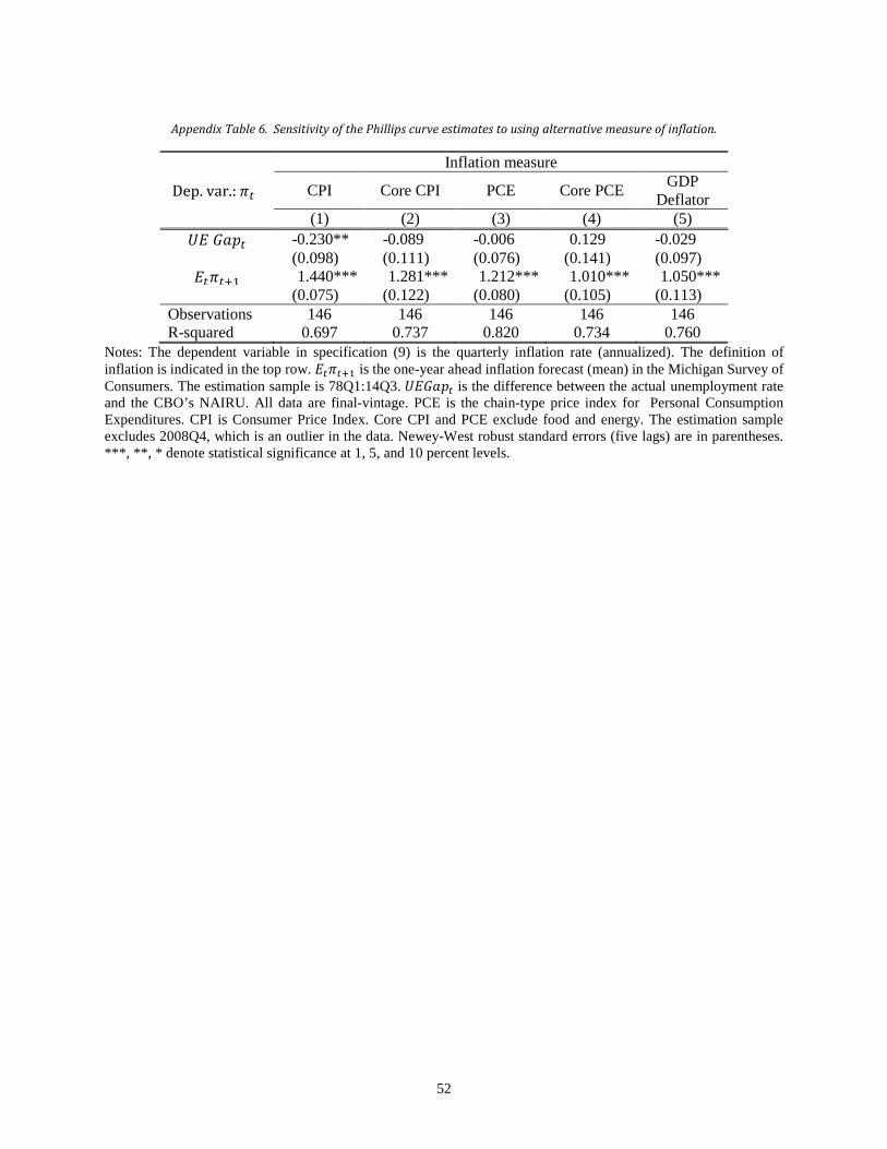
52

Appendix Table 6. Sensitivity of the Phillips curve estimates to using alternative measure of inflation.

Dep. var.: 𝜋𝜋𝑡𝑡

Inflation measure

CPI Core CPI PCE Core PCE GDP Deflator

(1) (2) (3) (4) (5) 𝑈𝑈𝐸𝐸 𝑈𝑈𝑎𝑎𝑝𝑝𝑡𝑡 -0.230** -0.089 -0.006 0.129 -0.029

(0.098) (0.111) (0.076) (0.141) (0.097) 𝐸𝐸𝑡𝑡𝜋𝜋𝑡𝑡+1 1.440*** 1.281*** 1.212*** 1.010*** 1.050***

(0.075) (0.122) (0.080) (0.105) (0.113) Observations 146 146 146 146 146 R-squared 0.697 0.737 0.820 0.734 0.760

Notes: The dependent variable in specification (9) is the quarterly inflation rate (annualized). The definition of inflation is indicated in the top row. 𝐸𝐸𝑡𝑡𝜋𝜋𝑡𝑡+1 is the one-year ahead inflation forecast (mean) in the Michigan Survey of Consumers. The estimation sample is 78Q1:14Q3. 𝑈𝑈𝐸𝐸𝑈𝑈𝑎𝑎𝑝𝑝𝑡𝑡 is the difference between the actual unemployment rate and the CBO’s NAIRU. All data are final-vintage. PCE is the chain-type price index for Personal Consumption Expenditures. CPI is Consumer Price Index. Core CPI and PCE exclude food and energy. The estimation sample excludes 2008Q4, which is an outlier in the data. Newey-West robust standard errors (five lags) are in parentheses. ***, **, * denote statistical significance at 1, 5, and 10 percent levels.

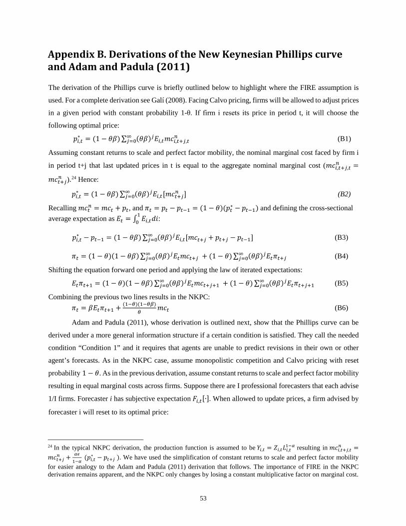
53

Appendix B. Derivations of the New Keynesian Phillips curve and Adam and Padula (2011) The derivation of the Phillips curve is briefly outlined below to highlight where the FIRE assumption is

used. For a complete derivation see Galí (2008). Facing Calvo pricing, firms will be allowed to adjust prices

in a given period with constant probability 1-θ. If firm i resets its price in period t, it will choose the

following optimal price:

𝑝𝑝𝑖𝑖,𝑡𝑡∗ = (1 − 𝜃𝜃𝛽𝛽)∑ (𝜃𝜃𝛽𝛽)𝑗𝑗𝐸𝐸𝑖𝑖,𝑡𝑡𝑚𝑚𝑜𝑜𝑖𝑖,𝑡𝑡+𝑗𝑗,𝑡𝑡𝑛𝑛 ∞

𝑗𝑗=0 (B1)

Assuming constant returns to scale and perfect factor mobility, the nominal marginal cost faced by firm i

in period t+j that last updated prices in t is equal to the aggregate nominal marginal cost (𝑚𝑚𝑜𝑜𝑖𝑖,𝑡𝑡+𝑗𝑗,𝑡𝑡𝑛𝑛 =

𝑚𝑚𝑜𝑜𝑡𝑡+𝑗𝑗𝑛𝑛 ).24 Hence:

𝑝𝑝𝑖𝑖,𝑡𝑡∗ = (1 − 𝜃𝜃𝛽𝛽)∑ (𝜃𝜃𝛽𝛽)𝑗𝑗𝐸𝐸𝑖𝑖,𝑡𝑡[𝑚𝑚𝑜𝑜𝑡𝑡+𝑗𝑗𝑛𝑛 ] ∞𝑗𝑗=0 (B2)

Recalling 𝑚𝑚𝑜𝑜𝑡𝑡𝑛𝑛 = 𝑚𝑚𝑜𝑜𝑡𝑡 + 𝑝𝑝𝑡𝑡, and 𝜋𝜋𝑡𝑡 = 𝑝𝑝𝑡𝑡 − 𝑝𝑝𝑡𝑡−1 = (1 − 𝜃𝜃)(𝑝𝑝𝑡𝑡∗ − 𝑝𝑝𝑡𝑡−1) and defining the cross-sectional average expectation as 𝐸𝐸𝑡𝑡 = ∫ 𝐸𝐸𝑖𝑖,𝑡𝑡𝑑𝑑𝑟𝑟

10 :

𝑝𝑝𝑖𝑖,𝑡𝑡∗ − 𝑝𝑝𝑡𝑡−1 = (1 − 𝜃𝜃𝛽𝛽)∑ (𝜃𝜃𝛽𝛽)𝑗𝑗𝐸𝐸𝑖𝑖,𝑡𝑡[𝑚𝑚𝑜𝑜𝑡𝑡+𝑗𝑗 + 𝑝𝑝𝑡𝑡+𝑗𝑗 − 𝑝𝑝𝑡𝑡−1] ∞

𝑗𝑗=0 (B3)

𝜋𝜋𝑡𝑡 = (1 − 𝜃𝜃)(1 − 𝜃𝜃𝛽𝛽)∑ (𝜃𝜃𝛽𝛽)𝑗𝑗𝐸𝐸𝑡𝑡𝑚𝑚𝑜𝑜𝑡𝑡+𝑗𝑗 ∞𝑗𝑗=0 + (1 − 𝜃𝜃)∑ (𝜃𝜃𝛽𝛽)𝑗𝑗𝐸𝐸𝑡𝑡𝜋𝜋𝑡𝑡+𝑗𝑗 ∞

𝑗𝑗=0 (B4)

Shifting the equation forward one period and applying the law of iterated expectations:

𝐸𝐸𝑡𝑡𝜋𝜋𝑡𝑡+1 = (1 − 𝜃𝜃)(1 − 𝜃𝜃𝛽𝛽)∑ (𝜃𝜃𝛽𝛽)𝑗𝑗𝐸𝐸𝑡𝑡𝑚𝑚𝑜𝑜𝑡𝑡+𝑗𝑗+1 ∞𝑗𝑗=0 + (1 − 𝜃𝜃)∑ (𝜃𝜃𝛽𝛽)𝑗𝑗𝐸𝐸𝑡𝑡𝜋𝜋𝑡𝑡+𝑗𝑗+1 ∞

𝑗𝑗=0 (B5)

Combining the previous two lines results in the NKPC: 𝜋𝜋𝑡𝑡 = 𝛽𝛽𝐸𝐸𝑡𝑡𝜋𝜋𝑡𝑡+1 + (1−𝜃𝜃)(1−𝜃𝜃𝜃𝜃)

𝜃𝜃𝑚𝑚𝑜𝑜𝑡𝑡 (B6)

Adam and Padula (2011), whose derivation is outlined next, show that the Phillips curve can be

derived under a more general information structure if a certain condition is satisfied. They call the needed

condition “Condition 1” and it requires that agents are unable to predict revisions in their own or other

agent’s forecasts. As in the NKPC case, assume monopolistic competition and Calvo pricing with reset

probability 1 − 𝜃𝜃. As in the previous derivation, assume constant returns to scale and perfect factor mobility

resulting in equal marginal costs across firms. Suppose there are I professional forecasters that each advise

1/I firms. Forecaster i has subjective expectation 𝐹𝐹𝑖𝑖,𝑡𝑡 [∙]. When allowed to update prices, a firm advised by

forecaster i will reset to its optimal price:

24 In the typical NKPC derivation, the production function is assumed to be 𝑌𝑌𝑖𝑖,𝑡𝑡 = 𝑍𝑍𝑖𝑖,𝑡𝑡𝐿𝐿𝑖𝑖,𝑡𝑡1−𝛼𝛼 resulting in 𝑚𝑚𝑜𝑜𝑖𝑖,𝑡𝑡+𝑗𝑗,𝑡𝑡

𝑛𝑛 =𝑚𝑚𝑜𝑜𝑡𝑡+𝑗𝑗𝑛𝑛 + 𝛼𝛼𝛼𝛼

1−𝛼𝛼 (𝑝𝑝𝑖𝑖,𝑡𝑡∗ − 𝑝𝑝𝑡𝑡+𝑗𝑗 ). We have used the simplification of constant returns to scale and perfect factor mobility

for easier analogy to the Adam and Padula (2011) derivation that follows. The importance of FIRE in the NKPC derivation remains apparent, and the NKPC only changes by losing a constant multiplicative factor on marginal cost.

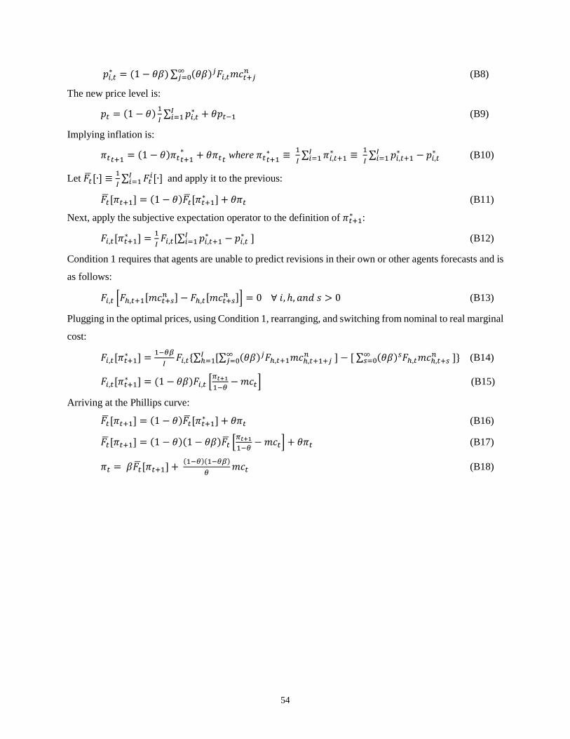
54

𝑝𝑝𝑖𝑖,𝑡𝑡∗ = (1 − 𝜃𝜃𝛽𝛽)∑ (𝜃𝜃𝛽𝛽)𝑗𝑗𝐹𝐹𝑖𝑖,𝑡𝑡𝑚𝑚𝑜𝑜𝑡𝑡+𝑗𝑗𝑛𝑛 ∞𝑗𝑗=0 (B8)

The new price level is:

𝑝𝑝𝑡𝑡 = (1 − 𝜃𝜃) 1𝐼𝐼∑ 𝑝𝑝𝑖𝑖,𝑡𝑡∗ + 𝜃𝜃𝑝𝑝𝑡𝑡−1𝐼𝐼𝑖𝑖=1 (B9)

Implying inflation is:

𝜋𝜋𝑡𝑡𝑡𝑡+1 = (1 − 𝜃𝜃)𝜋𝜋𝑡𝑡𝑡𝑡+1∗ + 𝜃𝜃𝜋𝜋𝑡𝑡𝑡𝑡 where 𝜋𝜋𝑡𝑡𝑡𝑡+1

∗ ≡ 1𝐼𝐼∑ 𝜋𝜋𝑖𝑖,𝑡𝑡+1∗ ≡ 1

𝐼𝐼∑ 𝑝𝑝𝑖𝑖,𝑡𝑡+1∗ − 𝑝𝑝𝑖𝑖,𝑡𝑡∗ 𝐼𝐼𝑖𝑖=1

𝐼𝐼𝑖𝑖=1 (B10)

Let 𝐹𝐹𝑡𝑡� [∙] ≡ 1𝐼𝐼∑ 𝐹𝐹𝑡𝑡𝑖𝑖[∙]𝐼𝐼𝑖𝑖=1 and apply it to the previous:

𝐹𝐹𝑡𝑡� [𝜋𝜋𝑡𝑡+1] = (1 − 𝜃𝜃)𝐹𝐹𝑡𝑡� [𝜋𝜋𝑡𝑡+1∗ ] + 𝜃𝜃𝜋𝜋𝑡𝑡 (B11)

Next, apply the subjective expectation operator to the definition of 𝜋𝜋𝑡𝑡+1∗ :

𝐹𝐹𝑖𝑖,𝑡𝑡[𝜋𝜋𝑡𝑡+1∗ ] = 1𝐼𝐼𝐹𝐹𝑖𝑖,𝑡𝑡[∑ 𝑝𝑝𝑖𝑖,𝑡𝑡+1∗ − 𝑝𝑝𝑖𝑖,𝑡𝑡∗ ]𝐼𝐼

𝑖𝑖=1 (B12)

Condition 1 requires that agents are unable to predict revisions in their own or other agents forecasts and is

as follows:

𝐹𝐹𝑖𝑖,𝑡𝑡 �𝐹𝐹ℎ,𝑡𝑡+1[𝑚𝑚𝑜𝑜𝑡𝑡+𝑠𝑠𝑛𝑛 ] − 𝐹𝐹ℎ,𝑡𝑡[𝑚𝑚𝑜𝑜𝑡𝑡+𝑠𝑠𝑛𝑛 ]� = 0 ∀ 𝑟𝑟,ℎ, 𝑎𝑎𝑎𝑎𝑑𝑑 𝑠𝑠 > 0 (B13)

Plugging in the optimal prices, using Condition 1, rearranging, and switching from nominal to real marginal

cost:

𝐹𝐹𝑖𝑖,𝑡𝑡[𝜋𝜋𝑡𝑡+1∗ ] = 1−𝜃𝜃𝜃𝜃𝐼𝐼

𝐹𝐹𝑖𝑖,𝑡𝑡{∑ [∑ (𝜃𝜃𝛽𝛽)𝑗𝑗𝐹𝐹ℎ,𝑡𝑡+1𝑚𝑚𝑜𝑜ℎ,𝑡𝑡+1+𝑗𝑗𝑛𝑛 ∞

𝑗𝑗=0 ] − [ ∑ (𝜃𝜃𝛽𝛽)𝑠𝑠𝐹𝐹ℎ,𝑡𝑡𝑚𝑚𝑜𝑜ℎ,𝑡𝑡+𝑠𝑠𝑛𝑛 ]∞

𝑠𝑠=0 }𝐼𝐼ℎ=1 (B14)

𝐹𝐹𝑖𝑖,𝑡𝑡[𝜋𝜋𝑡𝑡+1∗ ] = (1 − 𝜃𝜃𝛽𝛽)𝐹𝐹𝑖𝑖,𝑡𝑡 �𝜋𝜋𝑡𝑡+11−𝜃𝜃

−𝑚𝑚𝑜𝑜𝑡𝑡� (B15)

Arriving at the Phillips curve:

𝐹𝐹𝑡𝑡� [𝜋𝜋𝑡𝑡+1] = (1 − 𝜃𝜃)𝐹𝐹𝑡𝑡� [𝜋𝜋𝑡𝑡+1∗ ] + 𝜃𝜃𝜋𝜋𝑡𝑡 (B16)

𝐹𝐹𝑡𝑡� [𝜋𝜋𝑡𝑡+1] = (1 − 𝜃𝜃)(1− 𝜃𝜃𝛽𝛽)𝐹𝐹𝑡𝑡� �𝜋𝜋𝑡𝑡+11−𝜃𝜃

− 𝑚𝑚𝑜𝑜𝑡𝑡� + 𝜃𝜃𝜋𝜋𝑡𝑡 (B17)

𝜋𝜋𝑡𝑡 = 𝛽𝛽𝐹𝐹𝑡𝑡� [𝜋𝜋𝑡𝑡+1] + (1−𝜃𝜃)(1−𝜃𝜃𝜃𝜃)𝜃𝜃

𝑚𝑚𝑜𝑜𝑡𝑡 (B18)