THE FLORIDA STATE UNIVERSITY INTERNET …engelen/Arthi_Gokarn_Thesis.pdf · INTERNET COMPUTING WITH...
100
THE FLORIDA STATE UNIVERSITY COLLEGE OF ARTS AND SCIENCES INTERNET COMPUTING WITH MATLAB By ARTHI GOKARN A Thesis submitted to the Department of Computer Science in partial fulfillment of the requirements for the degree of Master of Science Degree Awarded: Summer Semester, 2004
Transcript of THE FLORIDA STATE UNIVERSITY INTERNET …engelen/Arthi_Gokarn_Thesis.pdf · INTERNET COMPUTING WITH...

THE FLORIDA STATE UNIVERSITY
COLLEGE OF ARTS AND SCIENCES
INTERNET COMPUTING WITH MATLAB
By
ARTHI GOKARN
A Thesis submitted to the
Department of Computer Science in partial fulfillment of the
requirements for the degree of Master of Science
Degree Awarded:
Summer Semester, 2004

The members of the committee approve the thesis of Arthi Gokarn, defended on July 14, 2004. _____________________
Robert A. van Engelen, Professor Directing Thesis
_____________________ Xin Yuan,
Committee member
_____________________ Lois Wright Hawkes,
Committee member
The Office of Graduate Studies has verified and approved the above named committee members.
ii

ACKNOWLEDGEMENTS
This thesis owes its existence to my major professor Dr. Robert van Engelen who showed
faith in me and gave me a great opportunity to do research under him. It is because of his
guidance and endurance that I was able to bring this thesis to the shape it currently is in.
I would also like to thank Dr. Lois Hawkes and Dr. Xin Yuan for serving in my graduate
committe and provide me valuable guidance in my academic coursework.
I feel indebted my friend and senior Prasad Kulkarni. It wouldn’t have been possible to
come to U.S.A. for graduate studies and complete the term of studies without his
guidance, support and encouragement.
My parent and sister have also been a great source of strength and support to me. I am
grateful to them for their perseverance, without which I couldn’t have imagined what life
would have been for me.
I would also like to thank all my friends in Tallahassee who provided invaluable support
throughout my graduate school and encouraged me when I need it most, in particular, I
would like to thank Virendra, Amit, Hemant, Deviprasad, Raju, Anu, Sandy, Vidya,
Jyoti, Mayank, and Raj.
iii

TABLE OF CONTENTS
INTRODUCTION .............................................................................................................. 1 SPARSE MATRIX REPRESENTATIONS....................................................................... 5
2.1 Sparse Matrices................................................................................................... 6 2.1.1 Definitions................................................................................................... 6 2.1.2 Nonzero Structures...................................................................................... 8 2.1.3 Sparse Storage Schemes ........................................................................... 11
MATLAB.......................................................................................................................... 25 3.1 Definition .......................................................................................................... 26 3.2 MATLAB interfaces ......................................................................................... 27
3.2.1 C MEX-Files............................................................................................. 27 3.3 Sparse Matrices................................................................................................. 31
3.3.1 Sparse Matrix Storage............................................................................... 31 3.3.2 Sparse matrices in gSOAP........................................................................ 32
XML WEB SERVICES.................................................................................................... 34 4.1 Web services ........................................................................................................... 36
4.1.1 Agents and Services......................................................................................... 36 4.1.2 Requesters and Providers................................................................................. 37 4.1.3 Service Description.......................................................................................... 37 4.1.4 Semantics ......................................................................................................... 37 4.1.5 Overview of Engaging a Web Service............................................................. 38
4.2 Web Services Technologies.................................................................................... 39 4.2.1 XML................................................................................................................. 41 4.2.2 SOAP ............................................................................................................... 43 4.2.3 WSDL .............................................................................................................. 44
4.3 Web Services and Scientific Computing ................................................................ 44 4.4 Data structures in SOAP and XML ........................................................................ 46
4.4.1 Simple Data Types........................................................................................... 47 4.4.2 Compound Data Types .................................................................................... 49
4.5 SOAP Encoded Arrays ........................................................................................... 50 4.5.1 Multi-dimensional Array .......................................................................... 51 4.5.2 Mixed Arrays ............................................................................................ 51 4.5.3 Sparse arrays ............................................................................................. 52
4.6 Miscellaneous Types............................................................................................... 53 4.6.1 Custom Encoding...................................................................................... 53 4.6.2 Multi-reference Values ............................................................................. 53
iv

4.6.3 Design of an XML Schema for Numeric Data ......................................... 55 4.7 SOAP Limitations............................................................................................. 57
DESIGN OF A WEB SERVICES COMPILER FOR MATLAB .................................... 58 5.1 Compilation....................................................................................................... 59 5.2 Execution .......................................................................................................... 63 5.3 Mapping of C data types to MATLAB data types. ........................................... 64 Implementation ............................................................................................................. 66
APPLICATIONS .............................................................................................................. 68 6.1 Visualizing the Mandelbrot Set ........................................................................ 68
6.1.1 Graphing the Mandelbrot set .................................................................... 69 6.1.2 Generating the MATLAB Interface.......................................................... 72
6.2 Weather Forecasting ......................................................................................... 74 6.2.1 Climate and Weather Forecast Models. .................................................... 75 6.2.2 Graphing the Weather Forecast Model ..................................................... 76 6.2.3 Invoking the MEX-File............................................................................. 77 6.2.4 Generating the MATLAB Interface.......................................................... 82
CONCLUSIONS............................................................................................................... 86 REFERENCES ................................................................................................................. 88 BIOGRAPHICAL SKETCH ........................................................................................... 93
v

LIST OF FIGURES
Figure 2-1: A square matrix.............................................................................................. 10 Figure 2-2: A band matrix................................................................................................. 12 Figure 2-3: Two ways of storing band matrix A............................................................... 12 Figure 2-4: A square matrix A. ......................................................................................... 13 Figure 2-5: A diagonal scheme for matrix A (Figure 2.4). ............................................... 14 Figure 2-6: A square matrix A. ......................................................................................... 15 Figure 2-7: Envelope Scheme........................................................................................... 16 Figure 2-8: A 5 x 5 square matrix..................................................................................... 16 Figure 2-9: Coordinate Scheme ........................................................................................ 17 Figure 2-10: Linked List Scheme ..................................................................................... 18 Figure 2-11: A 5 x 5 square matrix................................................................................... 19 Figure 2-12: Curtis and Reid Scheme............................................................................... 20 Figure 2-13: Sparse Row-wise Scheme ........................................................................... 22 Figure 2-14: Data Movement........................................................................................... 22 Figure 2-15: Extended Column Scheme .......................................................................... 23 Figure 2-16: Quad-Tree Representation .......................................................................... 24 Figure 3-1:C MEX Cycle.................................................................................................. 29 Figure 3-2: Mex function call. .......................................................................................... 30 Figure 4-1: The General Process of Engaging a Web Service.......................................... 39 Figure 4-2:Web Services Architecture Stack.................................................................... 40 Figure 5-1: Server-side code generation ........................................................................... 60 Figure 5-2: Client-side code generation............................................................................ 62 Figure 5-3: Execution ....................................................................................................... 63 Figure 6-1: Mandelbrot Set............................................................................................... 71 Figure 6-2: Pressure plot .................................................................................................. 79 Figure 6-3: Temperature plot ............................................................................................ 80 Figure 6-4: Wind velocity plot.......................................................................................... 81 Figure 6-5: HIRLAM forecast model ............................................................................... 82
vi

ABSTRACT
The purpose of this project is to create MATLAB applications that use the capabilities of
the World Wide Web to send data to a remote server for computation and to display the
results in on a local MATLAB® application. The data is sent to and received from the
remote application using gSOAP.
Data can be sent to a remote server, which need not have a copy of MATLAB installed.
This is accomplished by calling gSOAP functions from MEX-files written in the C
programming language. The MEX interface code and accompanying C code is
automatically generated by gSOAP. The use of the gSOAP compiler (which is part of this
project) simplifies this task, which otherwise requires users to program most of the data
communications at a lower level. This project specializes on efficient data representations
for communication with Web services, such as sparse numerical matrix representations.
The diagram shows the visualization of weather forecast data through MATLAB.
vii

CHAPTER 1
INTRODUCTION
The service-oriented architecture (SOA) is gaining momentum in research laboratories
and academia to establish collaborative research environments for distributed scientific
computing over the Internet. The SOA is an infrastructure strategy that relies on
middleware to connect applications. With the emergence of the Internet and a class of
middleware called XML Web services, SOA promises to automate software integration
and information sharing in all areas of computing, including scientific computing.
The Grid computing community recently adopted the SOA as its successor architecture
for Grid computing by publishing the Open Grid Service Architecture (OGSA), which is
essentially a SOA for Grid computing. OGSA was proposed by the Globus alliance and
efforts are under way to implement OGSA in the Globus toolkit. The result of this
achievement will be an infrastructure of middleware applications. The goal of this
infrastructure is to provide a toolset for developers to achieve interoperability among
large-scale scientific applications and to promote collaboration among researchers by
providing a uniform approach for data sharing.
Grid computing largely relies on middleware for connecting applications to solve large-
scale scientific and engineering problems in a distributed computing environment. While
the Grid community is starting to adopt the SOA strategy to enhance interoperability of
Grid applications by "wrapping" them in XML Web services for data sharing, not much
1

attention has been spent on automating this "wrapping" process and for choosing
bandwidth-efficient XML representations of scientific data to guarantee reasonable rates
of data throughput. In addition, the XML Web services standards such as the Simple
Object Access Protocol (SOAP) define the wrapper format but do not specify the process
of actually wrapping the scientific applications in Web services. Thus, there is sufficient
room to investigate, analyze, and compare approaches for the implementation of SOA-
based middleware toolkits for scientific applications.
The XML Web services standards are designed to address interoperability and security
issues in the SOA model. Interoperability is achieved by offering a rich set of extensible
XML-based data types for data sharing among disparate parties. The advantage of XML
Web services applications is platform independence. Contrast this to distributed and
parallel computing with the Message Passing Interface (MPI), which is popular among
scientific application developers. MPI is very much constrained by the availability of
libraries in the C and Fortran languages. The MPI library provides two application-
programming interfaces (APIs), one for C and one for Fortran. MPI efficiently manages
reliable connections between (virtual) compute nodes among many other pragmatic
issues. It also translates localized numerical representations between nodes, when
necessary. However, MPI and other message passing libraries and object-broker systems
such as CORBA and DCOM rely on reliable and secure connections and only achieve a
limited level of interoperability among applications developed with these specific
technologies.
One of the most popular tools for scientific computing is Matlab. It is used by scientists
and engineers to simulate dynamic processes or to visualize data sets by using Matlab's
graphical user interface. Simulation data is often available on a local disk. However,
when data has to be visualized from a remote location, FTP or GridFTP are typically used
to transport the data set to a local disk, for example from a supercomputer node in the
Grid. This manual process is error-prone and automation of FTP/GridFTP cannot be
easily integrated. Our proposed SOA approach eliminates explicit file transfers for
scientific computing with Matlab. Data providers and consumers act as XML Web
2

services to transport data to and from Matlab applications on demand. The goal of this
approach is to achieve interoperable data sharing in a dynamic environment, which
should be distinguished from approaches to parallelize Matlab applications to increase
simulation performance. Because Matlab supports (limited) sparse data structures, it is
also a suitable test bed environment to investigate and propose efficient XML
representations for sparse data structures.
This thesis investigates and implements a fully automated SOA approach for scientific
computing with large and/or sparse data sets in Matlab. The bandwidth requirements for
exchanging sparse numerical data sets can dramatically increase by orders of magnitude,
if the data is mapped to dense array representations in XML text form. To address this
concern, we implemented a mapping mechanism that exploits sparse array
representations in XML and compressed forms that preserve the precision of floating
point data.
For this investigation into methods for mapping sparse representations, we used gSOAP
[1] to develop a Web services interface for Matlab. GSOAP is a platform-independent
Web services development toolkit for C and C++. The toolkit maps C/C++ data types to
XML. To support sparse data representations, we developed custom XML encoders for
sparse and/or compressed data types. These encoders are integrated with Matlab. In
addition, the gSOAP compiler was extended in this project to automatically generate
application wrappers in Matlab code. By enhancing the gSOAP compiler to generate
Matlab code for wrapping in XML Web services, we automatically addressed the
interoperability problem without requiring users to write the required wrapper code.
Encryption mechanisms and user-authentication policies are not described in detail in this
thesis, because these are orthogonal to the Web services architecture, and are usually
enforced in the HTTP layer of the communication stack using SSL or in the XML layer
using the WS Security standards.
The XML Web services applications we developed for Matlab as a proof of concept are a
weather forecast application that produces data for visualization with Matlab and a server
3

that produces the Mandelbrot fractal data set for display with Matlab. The sparse XML
representations of the data used by these applications limits the communication latency of
SOAP/XML. The generalization of this approach to other scientific applications such as
atmospheric modeling, climate modeling and geographic information systems is
straightforward. With this approach we envision that Matlab applications can serve as a
scientific application drivers to control remote simulations, feed data back and forth to
these applications, and to visualize results on demand. Therefore, by developing an
efficient Web services interface for Matlab with gSOAP, users can orchestrate
collaborative numerical simulations for scientific experiments and visualize large data
sets.
The remainder of this thesis is organized as follows. Chapter 2 introduces sparse
matrices, which are common data representations found in scientific applications such as
PDE solvers. Chapter 3 presents Matlab and explains Matlab MEX files and the Matlab
MEX compiler to link C applications with Matlab code. The Matlab MEX interface is a
crucial component in our automated system. Data from Matlab is passed through the
MEX interface to the Web service application. Chapter 4 describes XML and Web
services standards, the basic data structures used in SOAP encoding, and our design of an
XML schema for numeric data. Chapter 5 explains the design and implementation of our
Web services compiler for Matlab. The compiler takes a Web Services Description
Language (WSDL) document and generates the C code and MEX files for the Matlab
MEX compiler to integrate the Web service functionality. Example applications and
results are explained in chapter 6. The thesis summarizes the conclusions in Chapter 7.
4

CHAPTER 2
SPARSE MATRIX REPRESENTATIONS
Numerical scientific and engineering applications typically involve handling of large-
scale numeric data sets to facilitate numerical simulations. The data used in scientific
applications are usually in the form of matrices and hence, sparse matrices are commonly
used for such applications. Most of the elements in these matrices are zero. For example,
such matrices can be produced either directly or indirectly by partial differential equation
(PDE) solvers.
Exploiting the occurrence of many zero elements in large sparse matrices may yield
substantial savings with respect to both the storage requirements and computational time
of numerical application. In the past, however, only limited compiler support has been
developed for sparse matrix computations and communication schemes.
If many elements in a matrix are zero, then this matrix is called a sparse matrix. In
contrast, a matrix containing many nonzero elements is referred to as dense matrix. Both
the storage requirements and computational time of an application that operates on sparse
matrices can be reduced substantially in comparison with an application that operates on
dense matrices by only storing nonzero elements and avoiding redundant operations on
zero elements.
5

In this chapter we discuss in some detail the effects of sparse matrices on storage space
and computational time. A number of sparse storage schemes will be introduced. In
particular, Matlab uses the “extended column or row scheme”. The gSOAP toolkit uses
the “coordinate scheme” for sparse matrix communication. This scheme is a natural
extension of the SOAP schema for SOAP encoded arrays, which supports the
representation of “sparse” multidimensional arrays. This project combines Matlab and
gSOAP to achieve interoperability between Matlab and non-Matlab applications using
effective numerical representations to limit communication latencies.
2.1 Sparse Matrices
In this section, we give definitions related to sparse matrices and identify some important
nonzero structures. Next, an overview of sparse storage schemes is given.
2.1.1 Definitions
If many elements in a matrix are zero, then this matrix is called a sparse matrix. Usually,
no attempts are made to obtain a more formal definition and we simply say that a matrix
is sparse if it contains sufficient zero elements to enable the exploitation of these zero
elements. Any other matrix is referred to as a dense matrix.
For an m by n sparse matrix A, the nonzero structure is defined as follows:
Nonz(A) = {(i, j) ∈ [1,m] x [1,n] | aij ≠ 0}
The number τ of nonzero elements in A is defined as τ = |Nonz(A)|. The density ρ of A is
defined as follows (giving rise to a sparsity of 1 - ρ):
ρ = τ / (m ⋅ n)
6
In many fields of science and engineering, applications arise that operate on sparse
matrices. Both the storage requirements and computational time of these applications can
be reduced substantially if advantage of the zero elements in these matrices is taken.
Reduction of Storage Requirements
Many sparse storage schemes have been developed to reduce the storage requirements of
a sparse matrix. Which sparse storage scheme is the most efficient heavily depends on
peculiarities of the nonzero structure of the sparse matrix and the kind of operations to be
applied to this matrix.
Storage required to store numerical values is called primary storage. Storage necessary to
reconstruct the underlying matrix is referred to as overhead storage. In some cases it is
practical to store some zero elements too, because the use of a simpler storage scheme
with less overhead storage compensates for the increase in the amount of primary storage
and results in less run-time overhead.
Elements that are stored explicitly are called entries. The set E(A) is used to indicate the
index set of all entries of a sparse m x n matrix A:
Nonz(A) ⊆ E(A) ⊆ [1,m] x [1,n]
Hence, (i, j) ∉ E(A) implies that aij = 0, but the converse implication does not necessarily
hold. Moreover, if elements of the matrix may change during a computation, we must be
ready to deal with situations in which zero elements become zero. Depending on whether
a fixed E(A) can be chosen such that Nonz(A) ⊆ E(A) will always hold during program
execution, or whether unpredictable alterations to E(A) must be possible at run-time, we
distinguish between static storage schemes and dynamic storage schemes.
For static storage schemes, we can further distinguish between cases where the fixed set
E(A) is already known at compile-time, because all changes are confined to fixed regions
7

known in advance, or where this fixed set E(A) is determined at run-time before
initialization of the storage scheme by computing a conservative approximation of
elements that may fill-in. In a dynamic storage scheme, we can alter the set E(A) at run-
time to account for the insertion of a new entry, which is referred to as creation. If
initially all zero elements in the matrix are exploited (viz. we start with E(A) = Nonz(A)),
then all fill-in induces creation. This can contribute substantially to the computational
time because data movement and occasionally a left compression may occur as explained
in section 2.1.3
Reduction of Computational Time
The actual time of an algorithm operating on a sparse matrix can be reduced if we
account for the fact that certain operations on zero elements can be skipped. Usually,
such a reduction of the actual computational time can only be achieved if an appropriate
storage scheme is used, because, in general, skipping operations by means of conditionals
does not yield a satisfactory reduction in computational time. Only if we can keep the
work proportional to the number of nonzero elements in a matrix, sparsity has been fully
exploited. Sparse storage schemes and related operations are further discussed in section
2.1.3
2.1.2 Nonzero Structures
We can distinguish between general sparse matrices and sparse matrices that have a
particular nonzero structure. In the following sections some important nonzero structures
of square matrices are identified (see e.g. [78, 173, 198, 199, 214]).
Band Forms
The lower semi-bandwidth bl and upper semi-bandwidth bu of a square n x n matrix A are
defined as the smallest integers bl ≥ 0 and bu ≥ 0 for which the following constraint is still
satisfied:
(aij ≠ 0) => (-bu ≤ i – j ≤ bl) (2.1)
8

Minimum values reveal the most information about the nonzero structure, because (2.1)
is trivially satisfied for bl = n – 1 and bu = n – 1. Allowing for negative semi-bandwidths
would enable the specification of an arbitrary band in which the main diagonal is not
necessarily included. However, usually we assume that all matrices have a full transversal
(i.e. all elements on the main diagonal are nonzero).
If the semi-bandwidths are relatively small, we say that the matrix is in band form, which
means that all nonzero elements are confined to a small band. The value bl + bu + 1 is
referred to as the bandwidth. Some special classes of band matrices can be distinguished.
A band matrix is in diagonal form if both bl and bu are zero, and in tridiagonal form if bl
= bu = 1. A band matrix A is in full band form if the following constraint is satisfied:
(-bu ≤ i – j ≤ bl) (aij ≠ 0)
The lower skyline li and upper skyline uj of an n x n matrix A with a full traversal are
defined as the following two sequences for 1 ≤ i ≤ n and 1 ≤ j ≤ n:
li = i - min {j | aij ≠ 0} (2.2)
uj = i - min {i | aij ≠ 0}
Each li and uj indicates the lowest and upper semi-bandwidth in the ith row and jth
column respectively:
(aij ≠ 0) => (-uj ≤ i – j ≤ li)
The lower and upper skyline defines the variable band form of a matrix. Although some
zero elements still appear within the variable band, the nonzero structure is described
more accurately by a variable band than by a band with fixed semi-bandwidths.
For a symmetric matrix A, i.e. a matrix that satisfies A = AT, the lower and upper skyline
are identical. The envelope of a symmetric matrix A consists of all elements in the
9

variable band that are below the main diagonal. The envelope size or profile p of A is
defined as follows [52, 97, 169]:
n p = ∑ li
i=1 Triangular Forms
A matrix satisfying the following constraint is in a lower triangular form:
(aij ≠ 0) => (j ≤ i )
If additionally, the equation aii = 1 holds for all 1 ≤ i ≤ n, then the matrix is in unit lower
triangular form. If the inequality is strict (viz. j < i, which implies that the traversal is
empty), then the matrix is in strictly lower triangular form. A lower triangular matrix is,
in fact, a special band matrix with bu = 0 and relatively large bl > 0. For a relatively small
bl > 0 the matrix is in so-called band lower triangular form. Similar definitions can be
given for matrices in (unit/strictly) upper triangular form and band upper triangular form.
Block Forms
Consider a block partition of a square matrix A (Figure 2-1) into sub-matrices Aij:
A … A11 1p
. . Ap1 App
A =
Figure 2-1: A square matrix
Each sub-matrix Aii, referred to as a diagonal block, is a square ni x ni sub-matrix. Hence
each sub-matrix Aij with i ≠ j, referred to as an off-diagonal block, is necessarily a ni x nj
sub-matrix. If a block consists of zero elements only, this is denoted by Aij = 0. Such
blocks are referred to as zero blocks.
10

Given this block partition, a block band form is defined by the block lower and upper
semi-bandwidths Bl ≥ 0 and Bu ≥ 0, which are the minimum values for which the
following constraint is still satisfied:
(Aij ≠ 0) => (-Bu ≤ i – j ≤ Bl)
If Bu = Bl = 1, then the matrix is in block tridiagonal form and we have a block diagonal
form if Bu = Bl = 0. For Bu = 0 and a relatively large Bl, the matrix is in block lower
triangular form. Likewise, for Bl = 0 and a relatively large Bu, the matrix is in block upper
triangular form. The off diagonal blocks Api and Aip for 1 ≤ i ≤ p are referred to as the
lower border and upper border respectively. If, except for some nonzero blocks in the
lower or upper form, a matrix is in block diagonal form, then the matrix is in doubly
bordered block diagonal form. Likewise, there are matrices in singly bordered block
lower triangular form or singly bordered block upper triangular.
2.1.3 Sparse Storage Schemes
In this section, we present some storage schemes for sparse matrices. We assume that the
constant N contains the order of the matrix to be stored. For dynamic data structures, we
assume that the value of a constant MAXSZ is at least the maximum number of entries
that can appear in this matrix.
Band and diagonal Schemes
In a band scheme [78,p200-203][97,p48-51][169,185,p13-14], all elements in the band of
a band matrix with the semi-bandwidths bl and bu are stored in a rectangular array
declared as either ‘REAL BND1 (N, BW)’ or ‘RAL BND2 (BW, N)’ in Fortran, where
BW=bl + bu + 1. Which of these declarations is used and the way in which entries are
stored in this array both depend on whether consecutive storage of the elements along
rows, columns or diagonals is desirable.
11

For example, consider the following 6 x 7 band matrix A as shown in Figure 2-2, having
bl = 2 and bu = 1:
a11 a12a21 a22 a23a31 a32 a33 a34 a42 a43 a44 a45
a53 a54 a55 a56 a64 a65 a66
A =
Figure 2-2: A band matrix
Two ways of storing the elements within the band of this matrix are illustrated in Figure
2-3 as shown below:
BND1
BND2
┴ ┴ a11 a12┴ a21 a22 a23 a31 a32 a33 a34 a42 a43 a44 a45 a53 a54 a55 a56 a64 a65 a66 ┴
┴ ┴ a31 a42 a53 a64┴ a21 a32 a43 a54 a65a11 a22 a33 a44 a55 a66 a12 a23 a34 a45 a56 ┴
Figure 2-3: Two ways of storing band matrix A.
For column-major storage, elements along one diagonal are stored consecutively in the
first rectangular array. The rows of A can be accessed along the rows of BND1 because
diagonals in the lower triangular part of A are down-justified, whereas all diagonals
above the main diagonal are up-justified in the array. Likewise, rows of A can be
accessed along the column of BND2 whereas diagonals of A are stored along the rows of
12

this array. However, other layouts are also possible.
Only the zero elements outside the band in the matrix are exploited using a band scheme,
because all elements within the band are stored explicitly (for symmetric band matrices
only the elements in the lower or upper triangular part of the band have to be stored):
E(A) = {(i,j) ∈ [1,m] x [1,n] | -bu ≤ i - j ≤ bl} ⊇ Nonz(A)
However, an advantage of this storage scheme is that, during LU-factorization without
pivoting (see appendix A), all fill-ins are confined to the band. Hence, the band scheme
can be used as static data structures in which creation does not have to be accounted for.
The relative simplicity of band schemes and the code operating on this data structure
together with the high performance that can be achieved on pipelined vector processors
have made band methods rather popular.
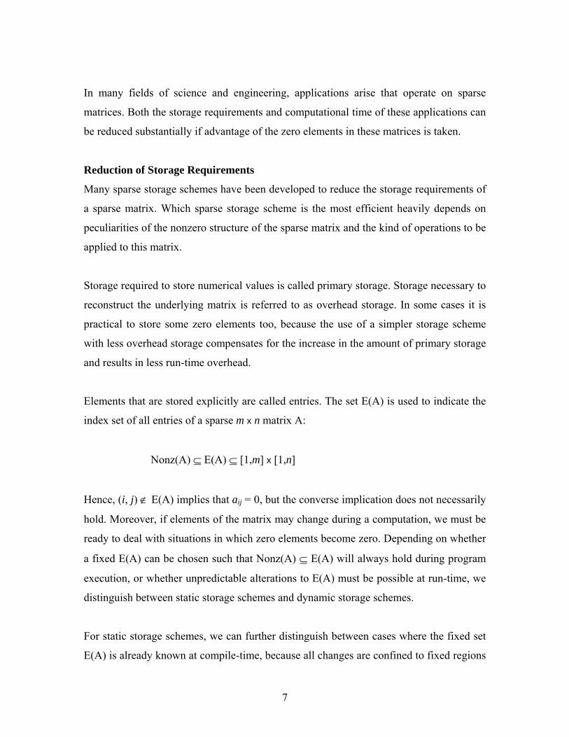
A slightly more complex variant of a band scheme that allows for storing a few nonzero
diagonals is formed by a diagonal scheme [185][129,ch11], where for each nonzero
diagonal an offset to the main diagonal is recorded in a one-dimensional array OFF,
while the diagonals are stored along the columns of a two-dimensional array VAL.
For example, consider the following 4 x 4 matrix A:
a11 a12
a22 a23 a31 a33 a34 a42 a44
A =
Figure 2-4: A square matrix A.
A diagonal scheme for this matrix is illustrated in Figure 2-5, below:
13
┴
a31
a42
a12
a23
a11
a22
a44
a33 a34
┴
┴2 0 -1OFF VAL
Figure 2-5: A diagonal scheme for matrix A (Figure 2-4).
Envelope schemes
Alternatively sparse storage schemes for symmetric band matrices that preserve most of
the simplicity of band schemes but at the same time offer more potential to exploit
sparsity are formed by envelope schemes [112,113]. These schemes are based on storage
of all elements in the lower triangular part that are within a variable band, i.e. E(A) is
defined as follows:
E(A) = {(i, j) ∈ [1,m] x [1,n] | -uj ≤ i - j ≤ li} ⊇ Nonz (A)
All elements in a row from the first nonzero element up to the diagonal element are
stored consecutively in a one-dimensional array, declared as ‘REAL VAL (MAXSZ)’ in
Fortran, in which the different row segments are stored contiguously. An additional one-
dimensional integer array, declared as ‘INTEGER PTR (N)’, is used to locate the
diagonal elements.
For example, consider the following lower triangular part of a symmetric and sparse 5 x 5
matrix A, where only the nonzero elements are shown:
14

a11 a21 a22 a23 a31 a33 a34
A =
Figure 2-6: A square matrix A.
The corresponding envelope storage scheme is illustrated in figure 2-7, where each
PTR(I) contains the location of the Ith diagonal element in the main sequence. An
element in the variable band with the row index I and column index J is stored at location
PTR(I)-I+J in the main sequence. Conversely, the column index of the first entry in row I
can be determined as follows:
I – (PTR(I) - PTR(I - 1) – 1)
Many variants of this storage scheme exist (see e.g. [78,p151-153, p204-205][96,p79-
80][146][169,p14-16][185]). The upper triangular part of the matrix can be stored by
columns, which corresponds to storing AT according to the previous method. Separate
storage can be used for the main diagonal. An advantage that is shared by all versions is
that, because during LU-factorization without pivoting, fill-in is confined to the variable
band, an envelope scheme can be used as static data structure. In fact, the envelope even
becomes completely full if a nonzero element appears before each diagonal element after
the first row [93].
15

Figure 2-7: Envelope Scheme
1 2 3 4 5
1 2 3 4 5 6 7 8 9 10 11 12VAL a21 a11 a55 a54 0 a52a44a43a330 a31a22
1 3 6 8 PTR 12
Coordinate schemes
The most convenient way to store a general sparse matrix is using a coordinate scheme,
in which all entries are stored as an unordered ser of triples (aij, i, j) in three parallel
arrays [78,p23-24][129, 185, 219][235, ch2].
For example, consider the following 5 x 5 matrix A, as shown in Figure 2-8:
a11 a14 a32 a44 a51 a55
A =
Figure 2-8: A 5 x 5 square matrix
The six nonzero elements of this matrix are stored in arbitrary order in the first six
elements of the parallel arrays VAL, ROW, and COL of size MAXSZ, as illustrated in
figure 2-9. A scalar SZ is used to record the number of explicitly stored elements. A new
16

entry can be easily entered at the first free location. A given entry can be easily deleted
by moving the last stored entry to the location of the deleted entry. However, in order to
search for a particular entry or to fetch an entire row or column, all entries must be
scanned, making this storage scheme less convenient for most numerical applications.
Due to its simplicity, coordinate schemes are used as input scheme by several
applications [74,80,94,164]. In this way, little constraints are imposed on the input sets.
The coordinate scheme is transformed into an efficient storage scheme before the actual
computations are performed.
a51
Linked list sc
A linked list
entry in its ro
first element
(2.3). A possi
same figure, i
a free-list, sho
REAL
INTEGER
INTEGER
For each entr
a55
5 11
14 5
2
3
4
1
4
5
Figure 2-9: Coordinate Schem
hemes:
scheme [122,p298-302] prov
ws as well as to the next e
in each list are stored. In f
ble implementation of the li
s shown below, where FRE
wn here in Fortran:
VAL(MAXSZ)
ROW(MAXSZ), COL(MA
HDR(N), HDC(N), FREE
y, the value, row and colum
1 2 3 4 5 6
VALROW
COL
a44
a14 a32 a11e
ides efficient access from each entry to the nest
ntry in its column. Furthermore, pointers to the
igure 2-10 this idea is illustrated for the matrix
nked list scheme [169,p16-20], illustrated in the
E can be used as a pointer to the first location of
XSZ), LNKR(MAXSZ), LNKC(MAXSZ)
n index together with links to the next entry in
17
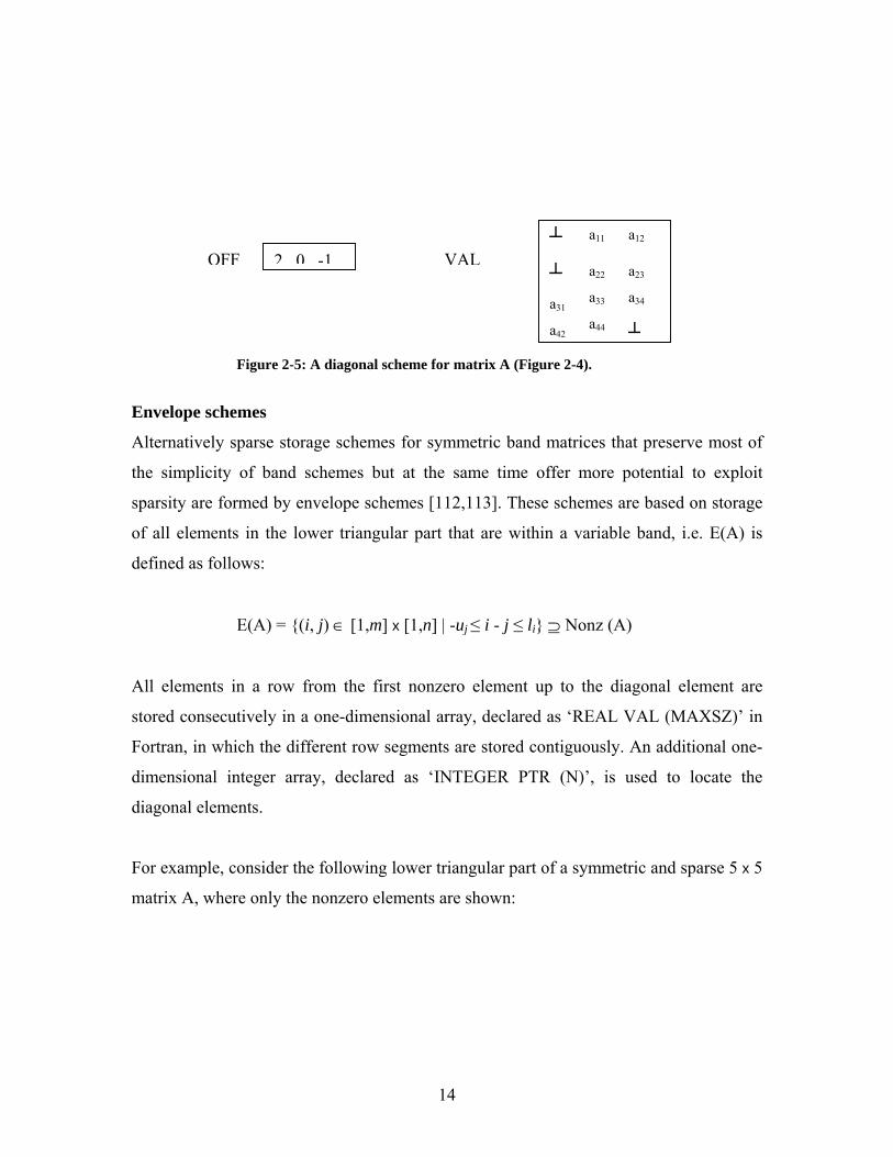
the same row and column are stored in five parallel arrays. Pointers to the location of the
first entry in each row and column can be found through the elements of arrays HDR and
HDC, respectively. For example, because in figure 2-6 we have HDR(5)=2, LNKR(2)=4,
and LNKR(4)=0, the entries in the 5th row can be found at locations 2 and 4 of the
parallel arrays. Obviously, because four integers are associated with each entry, this
storage scheme suffers from substantial overhead storage.
Some savings are obtained by dropping the row and column index associated with each
entry and replacing the null pointer at the end of each row and column list by the
negation of these indices [56][78,77,p31-32][235,p34-36]. This so-called Curtis and Reid
scheme is illustrated in figure 2-7. The row or column index of each entry is obtained by
scanning to the end of the row or column list. For sparse matrices having a small number
of entries in each row and column, the storage savings are obtained at the expense of only
a relatively small increase in computational time. Alternatively, storage can be saved if
only the entries in a row or a column are linked together, yielding a row-linked or
column-linked list [78,p28-29][185][199,ch1].
a11
a51 a55
a14
a32
a44
LNKR
LNKC
COL
ROW
VAL
6
5
4
2 0
11
1
a51a11
5
5
44
43
2
7 00 0
000 0
1
a44a14a32a55
1 2 3 4 5 6 7
4 2
6 7 5
5 0
0
1
1
HDCHDR
1 2 3 4 5
Figure 2-10: Linked List Scheme
18

The use of linked list scheme has an advantage that creation can be implemented without
any data movement, while only a few links are affected. Accessing the links, however,
may contribute substantially to the computation time, while locality may be distributed in
case the elements in a linked list are scattered through the parallel arrays.
General Sparse Row- or Column-wise Schemes
Another sparse storage scheme for general sparse matrices is based on storing either the
rows or columns as a set of sparse vectors.
For example, consider the 5 x 5 sparse matrix given below:
a11 a13 a14
a22 a25 a31 a33 a34
a41 a44 a53 a55
A =
Figure 2-11: A 5 x 5 square matrix
Sparse row-wise storage of A is illustrated in figure 2-12. The value of all entries in a row
together with the corresponding column indices are stored consecutively in the parallel
array VAL and IND, where entries in one row are not necessarily stored on column
index.
19

7
6 4
2
R
4
2
6 7 5
5 0 0
1 1
R
C C
Figure 2-12: Curtis and Reid Scheme
The location of the first entry in a row I can be found through PTR
of entries in this row is defined by LEN(I). A scalar FREE con
location at the end of all rows:
REAL VAL(MAXSZ)
INTEGER IND(MAXSZ), PTR(N), LEN(N), FREE
Inserting an element requires some data movement if there is no
the corresponding row. In this case, all entries of the row are mov
end of all rows, after which the new element is added. For examp
show the data structure of figure 2-13 after element a23 has been
row. The previously occupied locations are marked as free by re
indices. Free space can be used by subsequent insertions. In figure
new element can be inserted in row 1 or row 3 without any data m
data movement is required but cannot be done because insufficient
at the end of all rows, a left-compression is performed to make all r
[74,80][164,p23-33][235,p16-25]. Since such a left-compression is
sufficient working space must be supplied to prevent the situa
compression has to be applied many times.
There are different kinds of sparse row- and column-wise stora
[2][78,p24-25,p31-32][77,80][129,ch11][105,185][199,ch1][164][2
20
a55
7
VAL
(I), while the nu
tains the first un
free space adjace
ed to free space a
le, in figure 2-1
inserted in the se
setting the assoc
2-14, for instan
ovement. If, how
free space is ava
ows contiguous
relatively expen
tion in which a
ge schemes (see
35,ch2]).
a44
a14 a32 a111 2 3 4 5
HD HD1 2 3 4 5 6
LNK
LNK
a51
-1
-1
-5-5
-3
-4-4
-2mber
used
nt to
t the
4 we
cond
iated
ce , a
ever,
ilable
again
sive,
left-
e.g.
For
example, in ordered variants, the entries are stored on index information, making creation
slightly more expensive. An additional pointer can be used to separate entries in the
lower and triangular part, whereas the main diagonal can be kept in separate storage.
Because sparse row- or column-wise storage only supports fast generation of entries
along a row or column, the column- or row-structure of the matrix may be stored as well.
A representation of a sparse matrix in either a linked list scheme or the general sparse
scheme of this section can be efficiently converted into a similar representation of the
transposed matrix [106][169,p236-239]. In fact, since entries are ordered on index
information afterwards, applying such an algorithm twice can be used to convert an
unordered representation of a sparse matrix into an ordered representation
[8,106][169,p239-240].
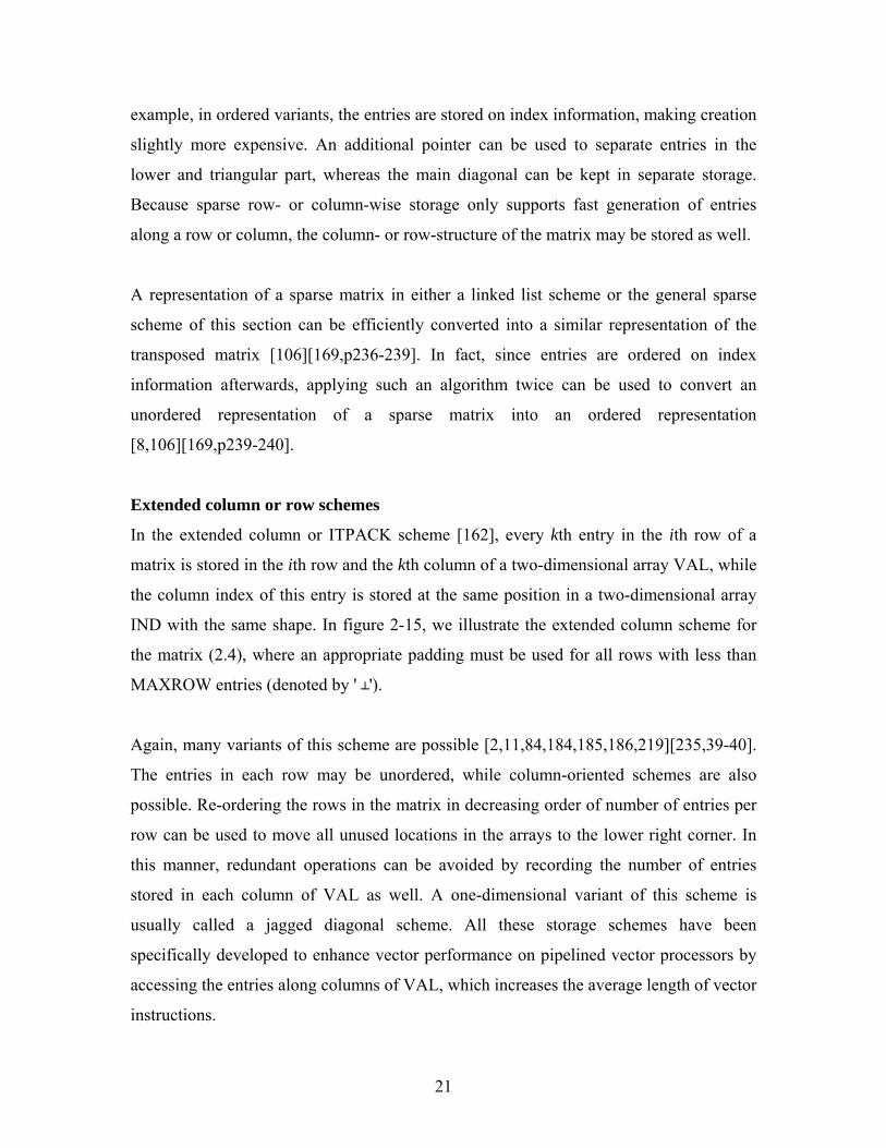
Extended column or row schemes
In the extended column or ITPACK scheme [162], every kth entry in the ith row of a
matrix is stored in the ith row and the kth column of a two-dimensional array VAL, while
the column index of this entry is stored at the same position in a two-dimensional array
IND with the same shape. In figure 2-15, we illustrate the extended column scheme for
the matrix (2.4), where an appropriate padding must be used for all rows with less than
MAXROW entries (denoted by ' ┴').
Again, many variants of this scheme are possible [2,11,84,184,185,186,219][235,39-40].
The entries in each row may be unordered, while column-oriented schemes are also
possible. Re-ordering the rows in the matrix in decreasing order of number of entries per
row can be used to move all unused locations in the arrays to the lower right corner. In
this manner, redundant operations can be avoided by recording the number of entries
stored in each column of VAL as well. A one-dimensional variant of this scheme is
usually called a jagged diagonal scheme. All these storage schemes have been
specifically developed to enhance vector performance on pipelined vector processors by
accessing the entries along columns of VAL, which increases the average length of vector
instructions.
21

2
9
23
4 6
2
1
3 R
4
3411 432 5 1 4 3
E
Figure 2-13: Sparse Row-wise Scheme
22333
R 1 63
0
-
1 4 3 3 41 1 4 3
0
9
Figure 2-14: Data Movement
22
a55
5
6
E
a55
35 2 5
VAL
VAL
a44
a44
a14
a14
a11
a11
1 2 3 4 5
1 2 3 4 5
-
LEN
LEN
PT
PT
11
11
1 2 3 4 5 6 7 8 9 10 11 12 13 1
IND
IND
FRE
FRE
a13
a13
a25
a25
a22
a22
a33
a33
a31
a31
a34
a34
a41
a41
a53
a53
1
1 2 3 4 5 6 7 8 9 10 11 12 13 14 15 1
a23
┴
┴
┴
┴
53
41
431
2 5
431IND
Fig
Quad- Tree schemes
As advocated in [1,220
image processing and
represent sparse matric
appropriate padding w
NULL-pointer, wherea
other matrices are repr
right-lower-, and right-
An example of a quad-
The quad-tree represen
as sparse matrices, wh
matrix partitioning. Fo
where the recursion te
scalars are encountere
using eight recursive m
nil pointer acts as mult
a55
VAL
a44
ure 2-
,221,
com
es. A
ith z
s a 1
esente
lower
tree r
tation
ile it
r exam
rmina
d. Lik
ultip
iplica
a14
a11┴ ┴
a13
a25
a22a33
a31 a34a41
a53
15: Extended Column Scheme
222,223], so called quad-trees, well-known from the fields of
puter graphics (see e.g. [110,ch10][191]) can be used to
n n x n matrix is embedded in a 2⎡ln n⎤ x 2⎡ln n⎤ matrix, where an
ero elements is applied. A zero matrix is represented by a
x 1 nonzero matrix is simple represented by a scalar. All
d as quadruple of sub-matrices consisting of the left-upper-,
-quadrant.
epresentation of a 4 x 4 sparse matrix is shown in figure 2-16.
provides a uniform way of representing both dense as well
also simplifies the implementation of algorithms based on
ple, the sum of two matrices can be assembled recursively,
tes if either one of the operands is the nil pointer, or if two
ewise, matrix multiplication can be formulated recursively
lications of quadrants followed by four additions, where the
tive cancellator and additive identity.
23

This concludes t
column or row sc
scheme. Part of
Matlab using gS
numerical data.
However, we wil
a44
a11
a22
a33
a21
a11 a22 a33 a44a21
Figure 2-16: Quad-Tree Representation
he chapter on sparse matrix representations. Matlab uses the extended
heme and the current version of the gSOAP toolkit uses the coordinate
this project is to design and implement a Web services interface for
OAP that supports sparse and other compressed representations of
The work specifically targets the extended column and row scheme.
l show that the approach supports other sparse representations as well.
24

CHAPTER 3
MATLAB
Many scientific applications include the visualization of large-scale numeric data. To
visualize numerical data, a wide range of tools is available, including Mathematica,
Maple, and MATLAB. These are popular symbolic and/or numerical mathematics
software packages that have their own strong points. We chose MATLAB for a number
of reasons. One of the reasons being the nature of the numerical data used in scientific
applications, while Maple and Mathematica are mainly intended for symbolic
computations. The data is usually in the form of matrices, and MATLAB performs vector
and matrix operations efficiently using sparse matrix representations. It is one of the most
popular tools used for efficient numerical computation combined with visualization.
One of the other reasons to use MATLAB is that it also provides interfaces to external
routines written in other programming languages like C. The ability to interface with C
makes it possible to communicate with remote applications. In this project, we have used
these features and have made it possible for MATLAB to do remote computations by
interfacing MATLAB with gSOAP. All data exchange is done through XML. XML
provides extendibility and interoperability. XML schema is provides a means to express
the data type definitions of sparse matrices, which are used extensively in scientific
applications.
25

Another reason for choosing MATLAB is that SOAP sparse matrices cannot be used with
the mathematical packages mentioned above.
Section 3.1 explains MATLAB. In section 3.2 we explain its interface with C as MEX-
files. Sparse matrices and its storage in MATLAB have been described in section 3.3. It
also discusses the representation of MATLAB sparse matrices in gSOAP, and the
functions associated with it.
3.1 Definition
MATLAB® is a high-performance language for technical computing. It integrates
computation, visualization, and programming in an easy-to-use environment where
problems and solutions are expressed in familiar mathematical notation. Typical uses
include
• Math and computation
• Algorithm development
• Data acquisition
• Modeling, simulation, and prototyping
• Data analysis, exploration, and visualization
• Scientific and engineering graphics
• Application development, including graphical user interface building
MATLAB is an interactive system whose basic data element is an array that does not
require dimensioning. This allows you to solve many technical computing problems,
especially those with matrix and vector formulations, in a fraction of the time it would
take to write a program in a scalar non-interactive language such as C or Fortran.
The MATLAB system consists of the following components:
26

The MATLAB Language. This is a high-level matrix/array language with control flow
statements, functions, data structures, input/output, and object-oriented programming
features. It allows both "programming in the small" to rapidly create “throwaway”
programs, and "programming in the large" to create complete large and complex
application programs.
The MATLAB Application Program Interface (API). This is a library that allows
you to write C and Fortran programs that interact with MATLAB. It includes facilities for
calling routines from MATLAB (dynamic linking), calling MATLAB as a computational
engine, and for reading and writing MAT-files.
It also consists of other components, which include the development environment, the
MATLAB Mathematical Functional Library and the Graphics component. We have made
extensive use of the interfaces provided by it for routines written in C, called MEX-files.
We explain about this is detail in the next section.
3.2 MATLAB interfaces
MATLAB® provides interfaces to external routines written in other programming
languages. It provides an interface to external programs written in the C language. C
subroutines can be called from MATLAB as if they were built-in functions. MATLAB
callable C programs are referred to as MEX-files. MEX-files are dynamically linked
subroutines that the MATLAB interpreter can automatically load and execute.
MEX-files have several applications:
• Large pre-existing C files can be called from MATLAB without having to be
rewritten as M-files.
27

• Bottleneck computations (usually for-loops) that do not run fast enough in
MATLAB can be recoded in C for efficiency.
3.2.1 C MEX-Files
C MEX-files are built by using the mex script to compile your C source code with
additional calls to API routines.
3.2.1.1 The Components of a C MEX-File
The source code for a MEX-file consists of two distinct parts:
• A computational routine that contains the code for performing the computations
that you want implemented in the MEX-file. Computations can be numerical
computations as well as inputting and outputting data.
• A gateway routine that interfaces the computational routine with MATLAB by
the entry point mexFunction and its parameters prhs, nrhs, plhs, nlhs, where
prhs is an array of right-hand input arguments, nrhs is the number of right-hand
input arguments, plhs is an array of left-hand output arguments, and nlhs is the
number of left-hand output arguments. The gateway calls the computational
routine as a subroutine.
In the gateway routine, you can access the data in the mxArray structure and then
manipulate this data in your C computational subroutine. For example, the expression
mxGetPr(prhs[0])returns a pointer of type double to the real data in the mxArray
pointed to by prhs[0]. You can then use this pointer like any other pointer of type
double in C. After calling your C computational routine from the gateway, you can set a
pointer of type mxArrayto the data it returns. MATLAB is then able to recognize the
output from your computational routine as the output from the MEX-file.
The following C MEX Cycle Figure 3-1 shows how inputs enter a MEX-file, what
functions the gateway routine performs, and how outputs return to MATLAB.
28

Figure 3-1:C MEX Cycle
3.2.1.2 Required Arguments to a MEX-File
The two components of the MEX-file may be separate or combined. In either case, the
files must contain the #include "mex.h" header so that the entry point and interface
routines are declared properly. The name of the gateway routine must always be
mexFunction and must contain these parameters. void mexFunction(
int nlhs, mxArray *plhs[],
int nrhs, const mxArray *prhs[])
{
/* more C code ... */
The parameters nlhs and nrhs contain the number of left- and right-hand arguments with
which the MEX-file is invoked. In the syntax of the MATLAB language, functions have
the general form
[a,b,c,...] = fun(d,e,f,...)
29

where the ellipsis (...) denotes additional terms of the same format. The a,b,c,... are
left-hand arguments and the d,e,f,... are right-hand arguments.
The parameters plhs and prhs are vectors that contain pointers to the left- and right-hand
arguments of the MEX-file. Note that both are declared as containing type mxArray *,
which means that the variables pointed at are MATLAB arrays. prhs is a length nrhs
array of pointers to the right-hand side inputs to the MEX-file, and plhs is a length nlhs
array that will contain pointers to the left-hand side outputs that your function generates.
For example, if you invoke a MEX-file from the MATLAB workspace with the
command x = fun(y,z);
the MATLAB interpreter calls mexFunction with the arguments as shown in Figure 3-2.
Figure 3-2: Mex function call.
plhs is a 1-element C array where the single element is a null pointer. prhs is a 2-
element C array where the first element is a pointer to an mxArray named Y and the
second element is a pointer to an mxArray named Z.
The parameter plhs points at nothing because the output x is not created until the
subroutine executes. It is the responsibility of the gateway routine to create an output
30

array and to set a pointer to that array in plhs[0]. If plhs[0] is left unassigned,
MATLAB prints a warning message stating that no output has been assigned.
3.3 Sparse Matrices
MATLAB supports sparse matrices, matrices that contain a small proportion of nonzero
elements. This characteristic provides advantages in both matrix storage space and
computation time. This section explains about the storage of sparse matrices in
MATLAB.
Sparse matrices are a special class of matrices that contain a significant number of zero-
valued elements. This property allows MATLAB to:
• Store only the nonzero elements of the matrix, together with their indices.
• Reduce computation time by eliminating operations on zero elements.
3.3.1 Sparse Matrix Storage
For full matrices, MATLAB stores internally every matrix element. Zero-valued elements
require the same amount of storage space as any other matrix element. For sparse
matrices, however, MATLAB stores only the nonzero elements and their indices. For
large matrices with a high percentage of zero-valued elements, this scheme significantly
reduces the amount of memory required for data storage.
MATLAB uses three arrays internally to store sparse matrices with real elements.
Consider an m-by-n sparse matrix with nnz nonzero entries stored in arrays of length
nzmax:
The first array contains all the nonzero elements of the array in floating-point format. The
length of this array is equal to nzmax.
31

The second array contains the corresponding integer row indices for the nonzero elements
stored in the first nnz entries. This array also has length equal to nzmax.
The third array contains n integer pointers to the start of each column in the other arrays
and an additional pointer that marks the end of those arrays. The length of the third array
is n+1.
This matrix requires storage for nzmax floating-point numbers and nzmax+n+1 integers.
At 8 bytes per floating-point number and 4 bytes per integer, the total number of bytes
required to store a sparse matrix is
8*nzmax + 4*(nzmax+n+1)
Sparse matrices with complex elements are also possible. In this case, MATLAB uses a
fourth array with nnz elements to store the imaginary parts of the nonzero elements. An
element is considered nonzero if either its real or imaginary part is nonzero.
3.3.2 Sparse matrices in gSOAP
The sparse function generates matrices in the MATLAB sparse storage organization. To
make use of these matrices in gSOAP we need to have a representation of them in
gSOAP. We declare a sparse matrix in gSOAP as:
struct soapSparseArray{
struct ArrayOfInt_soap_sparse ir;
struct ArrayOfInt_soap_sparse jc;
struct ArrayOfDouble_soap_sparse pr;
int num_columns;
int num_rows;
int nzmax;
};
32

The functions that operate on the sparse matrix are:
mxArray* c_to_mx_soapSparseArray(struct soapSparseArray);
mxArray* mx_to_c_soapSparseArray(const mxArray *, struct soapSparseArray *);
An instance of struct soapSparseArray needs to be created:
struct soapSparseArray x;
The mex file then makes use of the following functions to convert the sparse matrix
between its representation in MATLAB and C as:
mx_to_c_soapSparseArray(prhs[0],&x);
plhs[0] = c_to_mx_soapSparseArray(x);
33

CHAPTER 4
XML WEB SERVICES
The Web is a complex distributed system, and Object Technology has been an important
part of managing the complexity of the Web from its creation. Distributed object
technologies are exemplified by CORBA, DCOM and RMI. Web services on the other
hand, is a distributed system technology. Web services are based on XML documents and
document exchange. Exchanging documents is a very different concept from requesting
the instantiation of an object, requesting the invocation of a method on the specific object
instance, receiving the result of that invocation back in a response, and after a number of
these exchanges, releasing the object instance. The latter is used in distributed object
technologies.
Distributed object technology is very mature and robust, especially if you restrict its
usage to those environments, which it has been designed for: the corporate intranet with
often-homogenous platforms and predictable latencies. The strength of web services is in
the internet-style distributed computing, where interoperability and support for
heterogeneity in terms of platforms and networks are essential. Although, over time, web
services will need to incorporate some of the basic distributed systems technologies that
also underpin distributed object systems, such as guaranteed, in-order, exactly-once
message delivery, we have chosen web-services due to the above mentioned advantages.
Another reason for using web-services instead of any other distributed system
34

technologies, like CORBA, is that its ease of use. It is difficult to use CORBA, especially
with tools not designed for it, such as MATLAB.
Scientific applications typically deal with large symbolic or numerical data sets. The
paper “Pushing the SOAP Envelope With Web Services for Scientific Computing”,
addresses the usability, interoperability, and performance aspects of SOAP/XML Web
Services for scientific computing.
There are a number of SOAP Web Services toolkits and libraries for C/C++. Out of them
we chose to implement web services with the gSOAP toolkit. It is a platform-independent
development environment for C and C++ Web Services. Ease of use and performance
were important design considerations in the development of the toolkit. In fact, the toolkit
offers an easy-to-use RPC compiler that produces the stub and skeleton routines to
integrate (existing) C and C++ applications into SOAP/XML Web Services. A unique
aspect of the toolkit is that it automatically maps native C/C++ application data types to
semantically equivalent XML types and vice versa. This enables direct SOAP/XML
messaging with C/C++ applications on the Web. The overhead and memory usage of the
run-time mapping to XML with gSOAP’s schema-optimized XML parsing techniques is
low, which makes gSOAP attractive in high-performance environments and embedded
systems.
In this chapter we discuss about Web Services, its technologies in sections 4.1 and 4.2
respectively. Scientific Computing is one of the most important applications of web
services. This has been discussed about in section 4.5. Section 4.4 describes about the
various data structures used in SOAP and XML. SOAP Encoded arrays have been
explained in Section 4.5. Data types that do no to fall in the above mentioned categories
are covered in section 4.6. There are a few limitations in SOAP1.1 which are elaborated
in section 4.7.
35

4.1 Web services
Web services provide a standard means of interoperating between different software
applications, running on a variety of platforms and/or frameworks. The Web Service
Architecture (WSA) is intended to provide a common definition of a Web service, and
define its place within a larger Web services framework to guide the community. The
WSA provides a conceptual model and a context for understanding Web services and the
relationships between the components of this model.
The architecture does not attempt to specify how Web services are implemented, and
imposes no restriction on how Web services might be combined. The WSA describes
both the minimal characteristics that are common to all Web services, and a number of
characteristics that are needed by many, but not all, Web services.
The Web services architecture is an interoperability architecture: it identifies those global
elements of the global Web services network that are required in order to ensure
interoperability between Web services.
WSA provides the following definition:
[Definition: A Web service is a software system designed to support interoperable
machine-to-machine interaction over a network. It has an interface described in a
machine-processable format (specifically WSDL). Other systems interact with the Web
service in a manner prescribed by its description using SOAP messages, typically
conveyed using HTTP with an XML serialization in conjunction with other Web-related
standards.]
4.1.1 Agents and Services
A Web service is an abstract notion that must be implemented by a concrete agent. (See
Figure 4-1) The agent is the concrete piece of software or hardware that sends and
36

receives messages, while the service is the resource characterized by the abstract set of
functionality that is provided.
4.1.2 Requesters and Providers
The purpose of a Web service is to provide some functionality on behalf of its owner -- a
person or organization, such as a business or an individual. The provider entity is the
person or organization that provides an appropriate agent to implement a particular
service. (See Figure 4-1: Basic Architectural Roles.)
A requester entity is a person or organization that wishes to make use of a provider
entity's Web service. It will use a requester agent to exchange messages with the provider
entity's provider agent.
In order for this message exchange to be successful, the requester entity and the provider
entity must first agree on both the semantics and the mechanics of the message exchange.
4.1.3 Service Description
The mechanics of the message exchange are documented in a Web service description
(WSD). (See Figure 4-1) The WSD is a machine-processable specification of the Web
service's interface, written in WSDL. It defines the message formats, datatypes, transport
protocols, and transport serialization formats that should be used between the requester
agent and the provider agent. It also specifies one or more network locations at which a
provider agent can be invoked, and may provide some information about the message
exchange pattern that is expected. In essence, the service description represents an
agreement governing the mechanics of interacting with that service.
4.1.4 Semantics
The semantics of a Web service is the shared expectation about the behavior of the
service, in particular in response to messages that are sent to it. In effect, this is the
37

"contract" between the requester entity and the provider entity regarding the purpose and
consequences of the interaction. Although this contract represents the overall agreement
between the requester entity and the provider entity on how and why their respective
agents will interact, it is not necessarily written or explicitly negotiated. It may be explicit
or implicit, oral or written, machine processable or human oriented, and it may be a legal
agreement or an informal (non-legal) agreement.
While the service description represents a contract governing the mechanics of
interacting with a particular service, the semantics represents a contract governing the
meaning and purpose of that interaction. The dividing line between these two is not
necessarily rigid. As more semantically rich languages are used to describe the mechanics
of the interaction, more of the essential information may migrate from the informal
semantics to the service description. As this migration occurs, more of the work required
to achieve successful interaction can be automated.
4.1.5 Overview of Engaging a Web Service
There are many ways that a requester entity might engage and use a Web service. In
general, the following broad steps are required, as illustrated in Figure 4-1: (1) the
requester and provider entities become known to each other (or at least one becomes
know to the other); (2) the requester and provider entities agree on the service description
and semantics that will govern the interaction between the requester and provider agents;
(3) the service description and semantics are realized by the requester and provider
agents; and (4) the requester and provider agents exchange messages, thus performing
some task on behalf of the requester and provider entities. (i.e., the exchange of messages
with the provider agent represents the concrete manifestation of interacting with the
provider entity's Web service.) Some of these steps may be automated, others may be
performed manually.
38

Figure 4-1: The General Process of Engaging a Web Service
4.2 Web Services Technologies
Web service architecture involves many layered and interrelated technologies. There are
many ways to visualize these technologies. Figure 4-2 below provides one illustration of
some of these technology families.
39

Figure 4-2:Web Services Architecture Stack
This section describes some of those technologies that seem critical and the role they fill
in relation to this architecture. The technologies considered here, in relation to the
Architecture, are XML, SOAP, WSDL. However, there are many other technologies that
may be useful.
40

4.2.1 XML
XML solves a key technology requirement that appears in many places. By offering a
standard, flexible and inherently extensible data format, XML significantly reduces the
burden of deploying the many technologies needed to ensure the success of Web services.
With XML, data can be exchanged between incompatible systems. In the real world,
computer systems and databases contain data in incompatible formats. One of the most
time-consuming challenges for developers has been to exchange data between such
systems over the Internet. Automatically converting the data to XML can greatly reduce
this complexity and create data that can be read by many different types of applications.
The important aspects of XML, for the purposes of this architecture, are the core syntax
itself, the concepts of the XML Infoset, XML Schema and XML Namespaces.
XML Infoset is not a data format per se, but a formal set of information items and their
associated properties that comprise an abstract description of an XML document. The
XML Infoset specification provides for a consistent and rigorous set of definitions for use
in other specifications that need to refer to the information in a well-formed XML
document.
Serialization of the XML Infoset definitions of information may be expressed using XML
1.0. However, this is not an inherent requirement of the architecture. The flexibility in
choice of serialization format(s) allows for broader interoperability between agents in the
system. In the future, a binary encoding of the XML infoset may be a suitable
replacement for the textual serialization. Such a binary encoding may be more efficient
and more suitable for machine-to-machine interactions.
An XML schema describes the structure of an XML document. The XML Schema
language is also referred to as XML Schema Definition (XSD). The purpose of an XML
Schema is to define the legal building blocks of an XML document.
41
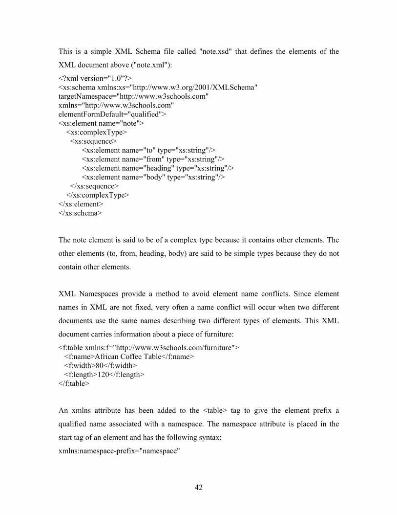
This is a simple XML Schema file called "note.xsd" that defines the elements of the
XML document above ("note.xml"):
<?xml version="1.0"?> <xs:schema xmlns:xs="http://www.w3.org/2001/XMLSchema" targetNamespace="http://www.w3schools.com" xmlns="http://www.w3schools.com" elementFormDefault="qualified"> <xs:element name="note"> <xs:complexType> <xs:sequence> <xs:element name="to" type="xs:string"/> <xs:element name="from" type="xs:string"/> <xs:element name="heading" type="xs:string"/> <xs:element name="body" type="xs:string"/> </xs:sequence> </xs:complexType> </xs:element> </xs:schema>
The note element is said to be of a complex type because it contains other elements. The
other elements (to, from, heading, body) are said to be simple types because they do not
contain other elements.
XML Namespaces provide a method to avoid element name conflicts. Since element
names in XML are not fixed, very often a name conflict will occur when two different
documents use the same names describing two different types of elements. This XML
document carries information about a piece of furniture:
<f:table xmlns:f="http://www.w3schools.com/furniture"> <f:name>African Coffee Table</f:name> <f:width>80</f:width> <f:length>120</f:length> </f:table>
An xmlns attribute has been added to the <table> tag to give the element prefix a
qualified name associated with a namespace. The namespace attribute is placed in the
start tag of an element and has the following syntax:
xmlns:namespace-prefix="namespace"
42

In the examples above, the namespace itself is defined using an Internet address:
xmlns:f="http://www.w3schools.com/furniture"
The W3C namespace specification states that the namespace itself should be a Uniform
Resource Identifier (URI).
4.2.2 SOAP
SOAP 1.2 provides a standard, extensible, composable framework for packaging and
exchanging XML messages. In the context of this architecture, SOAP 1.2 also provides a
convenient mechanism for referencing capabilities (typically by use of headers).
[SOAP 1.2 Part 1] defines an XML-based messaging framework: a processing model and
an exensibility model. SOAP messages can be carried by a variety of network protocols;
such as HTTP, SMTP, FTP, RMI/IIOP, or a proprietary messaging protocol.
[SOAP 1.2 Part 2] defines three optional components: a set of encoding rules for
expressing instances of application-defined data types, a convention for representing
remote procedure calls (RPC) and responses, and a set of rules for using SOAP with
HTTP/1.1.
While SOAP Version 1.2 [SOAP 1.2 Part 1] doesn't define "SOAP" as an acronym
anymore, there are two expansions of the term that reflect these different ways in which
the technology can be interpreted:
Service Oriented Architecture Protocol: In the general case, a SOAP message represents
the information needed to invoke a service or reflect the results of a service invocation,
and contains the information specified in the service interface definition.
Simple Object Access Protocol: When using the optional SOAP RPC Representation, a
SOAP message represents a method invocation on a remote object, and the serialization
of in the argument list of that method that must be moved from the local environment to
the remote environment.
43
SOAP messages are typically conveyed using HTTP as the network protocol. Today's
applications communicate using Remote Procedure Calls (RPC) between objects like
DCOM and CORBA, but HTTP was not designed for this. RPC represents a
compatibility and security problem; firewalls and proxy servers will normally block this
kind of traffic.
A better way to communicate between applications is over HTTP, because all Internet
browsers and servers support HTTP. SOAP was created to accomplish this. HTTP-related
protocols can be used to achieve authentication, security, compression, and so on.
4.2.3 WSDL
WSDL 2.0[WSDL 2.0 Part 1] is a language for describing Web services. WSDL
describes Web services starting with the messages that are exchanged between the
requester and provider agents. It is an XML based language. The messages themselves
are described abstractly and then bound to a concrete network protocol and message
format.
Web service definitions can be mapped to any implementation language, platform, object
model, or messaging system. Simple extensions to existing Internet infrastructure can
implement Web services for interaction via browsers or directly within an application.
The application could be implemented using COM, JMS, CORBA, or any number of
proprietary integration solutions. As long as both the sender and receiver agree on the
service description, (e.g. WSDL file), the implementations behind the Web services can
be anything.
44

4.3 Web Services and Scientific Computing
Scientific Computing is the collection of tools, techniques and theories required to
develop and solve on a computer, mathematical models in science and engineering.
Modeling new designs on a computer can save millions of dollars compared to building a
series of prototypes. An example of this is weather predictions used by meteorologists.
The growing synergy between Web Services and Grid based technologies will potentially
enable profound, dynamic interactions between scientific applications dispersed in
geographic, institutional, and conceptual space. Such deep interoperability requires the
simplicity, robustness, and extensibility for which SOAP was conceived, thus making it a
natural lingua franca.
Large arrays are common objects in scientific computing. Kenneth Chiu, in his paper
“Investigating the Limits of SOAP Performance for Scientific Computing”, demonstrated
that 90% of the overhead for numerical arrays is spent converting between decimals
formats in XML for floating point data. Thus, it is essential to limit the size of floating
point data and/or use other representations when performance is critical.
A common trade-off in computing is between the needs of universality and high
performance. The qualities of SOAP that make it universally usable tend to work against
high performance communications. In particular, XML specifies a primarily ASCII
format. A characteristic that distinguishes scientific and engineering components is the
need to frequently exchange large arrays of floating point numbers, with full accuracy to
assure reproducibility. Scientific computing also demands the full range of capabilities
that industrial computing does: reliable transfer in distributed heterogeneous
environments, parallel programs sending large, complex and rapidly changing data
objects or self-contained modules sending events to steer other modules, and complex
run-time systems designed for heterogeneous environments with dynamically varying
45

loads, multiple communication protocols, and differing Quality of Service (QoS)
requirements.
A Web Services approach to scientific components would allow users to combine the
strengths of different systems by developing applications that have components from
several of them. Since these systems can be connected via more than one protocol, a
common denominator protocol is needed to negotiate more specialized protocols. This
common denominator protocol must provide reliability, robustness, readability, ease of
use, seamless integration with existing computational code and interoperability. It is
shown that SOAP can be used to meet this criterion.
In order to build SOAP messages from a language of choice, we need to know how to
serialize data. We need to know the rules for representing an integer, string, or floating
point number in a SOAP message so that we can exchange messages freely between
languages and platforms. The serialization of data inside a SOAP message is referred to
as encoding. The next section focuses on the payload of the message. The XML in the
examples represents only a SOAP message payload and not a complete message.
4.4 Data structures in SOAP and XML
The ability to decide on a set of rules for representing data in a message is very important
to the open nature of SOAP. The encodingStyle attribute defined by the SOAP
specification is used to identify the encoding rules used in a particular message.
Encoding can make use of XML Schemas. In the case of SOAP encoding, the URI used
in the encodingStyle attribute points to a schema. The SOAP encoding rules use XML
Schemas heavily, relying on the XML Schema data types namespace and the type
46

attribute. Encoding does not mandate XML Schemas. This allows developers who do not
necessarily need the capabilities of XML Schemas to forego their use.
The SOAP Specification defines a single set of encoding rules that are referred to as
SOAP encoding. SOAP encoding is based on XML Schemas. The value of the
encodingStyle attribute for SOAP encoding is
http://schemas.xmlsoap.org/soap/encoding/, which points to the XML Schema that
defines the encoding rules.
4.4.1 Simple Data Types
In SOAP encoding, simple types are always represented as single elements in the body.
SOAP encoding exposes all the simple types that are built into the XML Schemas
Specification. If we are using a simple type with SOAP encoding, then it must come from
XML Schemas, or be derived from a type that does. The namespace associated with the
XML Schemas data types is http://www.w3.org/2001/XMLSchema. This provides the
common types that many programmers will expect, like: string, integer, float, date, and so
on. If we assume the xsd prefix is associated with the XML Schemas URI, and the
soapENC prefix is associated with the SOAP encoding URI, then both of these payload
values work with strings. This refers to XML Schemas:
<codename xsi:type="xsd:string">Hulk</codename>
while this refers to SOAP encoding:
<codename xsi:type="soapENC:string">Hulk</codename>
4.4.1.1 Enumerations
SOAP encoding allows us to define enumerated types. It borrows once again from XML
Schemas, which also has the concept of an enumeration. An enumeration is a named set
of values, based on a basic type. For example, we could define an enumeration that
represented geographical locations ("North, "South", etc). To define an enumeration, we
must use XML Schemas.
Here is an example of an enumeration that defines a set of geographical regions.
47

<simpleType name="Region" base="xsd:string"> <enumeration value="North"/> <enumeration value="South"/> <enumeration value="East"/> <enumeration value="West"/> </simpleType>
If this enumeration appeared in a referenced schema, we could then use this type in a
SOAP message just as we would any other type.
<soap:Envelope xmlns:soap="http://schemas.xmlsoap.org/soap/envelope/" soap:encodingStyle="http://schemas.xmlsoap.org/soap /encoding/" xmlns:xsi="http://www.w3.org/1999/XMLSchema-instance"> <soap:Body> <m:GetSalesTotals xmlns:m="http://www.wrox.com/sales/"> <m:reg xsi:type="m:Region">East</m:reg> </m:GetSalesTotals> </soap:Body> </soap:Envelope> 4.4.1.2 Binary Data
As part of the simple types it supports, SOAP and XML Schemas provide a type for
representing binary data. One approach for working with binary data is to use the base64
type. We can represent binary data, such as an image file, as an array of bytes in the
message. The base64 type converts binary data to text using the base64-encoding
algorithm of XML Schemas. There is no relationship between SOAP and base64-
encoding; if we use it, our application (or implementation of SOAP for your platform)
must be able to understand and work with base64-encoding.
In addition to the simple types, many languages have a "universal" data type or
placeholder, something that can represent a variety of types within that language. SOAP
accounts for this possibility with the polymorphic accessor. If we are serializing a value
in the form of a polymorphic accessor, we must provide the type attribute.
Assume that we are passing in a value representing a person's age, and that type could
vary depending on how the information was to be used. If the value of our data is a float,
it would appear like this:
48

<age xsi:type="xsd:float">3.5</age>
If is a string, it would appear like this:
<age xsi:type="xsd:string">3 and a half years old</age>
Both examples are legal if the age element has been defined as being a polymorphic
accessor, meaning that its data type will vary.
4.4.2 Compound Data Types
SOAP encoding provides structures for representing compound types. SOAP encoding
handles two compound types: structs (records), and arrays. Complex types are serialized
as payload elements, just like simple types, but they have child elements. The child
elements are the fields or elements of the type. SOAP had to invent its own rules for
structs and arrays because, as of this writing, XML Schemas does not pay special
attention to these compound types.
4.4.2.1 Structs
A struct (or structure, or record) is easy to represent as XML, because it has unique
named members. Consider this C++ struct definition of a super-hero:
struct SuperHero { string sCodename; string sFirstName; string sLastName; int nAge; }; SuperHero hero = { "Hulk", "Bruce", "Banner", 32 };
We've chosen a simple struct to illustrate the basics of compound types. If we serialize
the variable "hero" into a SOAP message payload using SOAP encoding, it would look
like this:
<hero xsi:type="x:SuperHero"> <sCodeName xsi:type="xsd:string">Hulk</sCodeName> <sFirstName xsi:type="xsd:string">Bruce</sFirstName> <sLastName xsi:type="xsd:string">Banner</sLastName> <nAge xsi:type="xsd:integer">32</nAge> </hero>
49

As can be seen in this example, the xsi:type attribute is used on compound data types as
well as simple types. In this case, the type is x:SuperHero, and the x namespace would
point to a schema that represents our SuperHero struct.
4.4.2.2 Arrays
Arrays are compound types as well, and they are represented in much the same way that
structs are. As we might expect, the difference between arrays and structs is in how we
refer to their members. Structs have data that is identifiable by name, and array members
are identified by position. The names of array elements are insignificant, so they cannot
be used to look up a value. In SOAP encoding, arrays are considered a special type. This
has been discussed in detail in the following section.
4.5 SOAP Encoded Arrays
This type is indicated by their xsi:type attribute, which is SOAP-ENC:Array. As with all
SOAP encoding, the namespace associated with the Array type is
http://schemas.xmlsoap.org/soap/encoding. Elements with this xsi:type are declared as
SOAP encoding arrays. The type of the array members is declared using another
attribute, SOAP-ENC:arrayType. This attribute indicates the type and size of the array.
Arrays in SOAP encoding can be confusing, so let's take a look at a simple array of five
integers to see how these attributes are used to define an array:
<numbers xsi:type="SOAP-ENC:Array" SOAP-ENC:arrayType="xsd:integer[5]"> <item>10</item> <item>20</item> <item>30</item> <item>40</item> <item>50</item> </numbers>
50
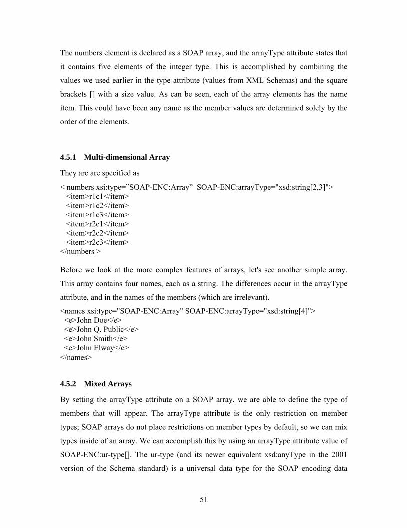
The numbers element is declared as a SOAP array, and the arrayType attribute states that
it contains five elements of the integer type. This is accomplished by combining the
values we used earlier in the type attribute (values from XML Schemas) and the square
brackets [] with a size value. As can be seen, each of the array elements has the name
item. This could have been any name as the member values are determined solely by the
order of the elements.
4.5.1 Multi-dimensional Array
They are are specified as
< numbers xsi:type=”SOAP-ENC:Array” SOAP-ENC:arrayType="xsd:string[2,3]"> <item>r1c1</item> <item>r1c2</item> <item>r1c3</item> <item>r2c1</item> <item>r2c2</item> <item>r2c3</item> </numbers > Before we look at the more complex features of arrays, let's see another simple array.
This array contains four names, each as a string. The differences occur in the arrayType
attribute, and in the names of the members (which are irrelevant).
<names xsi:type="SOAP-ENC:Array" SOAP-ENC:arrayType="xsd:string[4]"> <e>John Doe</e> <e>John Q. Public</e> <e>John Smith</e> <e>John Elway</e> </names>
4.5.2 Mixed Arrays
By setting the arrayType attribute on a SOAP array, we are able to define the type of
members that will appear. The arrayType attribute is the only restriction on member
types; SOAP arrays do not place restrictions on member types by default, so we can mix
types inside of an array. We can accomplish this by using an arrayType attribute value of
SOAP-ENC:ur-type[]. The ur-type (and its newer equivalent xsd:anyType in the 2001
version of the Schema standard) is a universal data type for the SOAP encoding data
51
types, so arrays that use this can have mixed members. The only catch to using ur-type[]
is that like the polymorphic accessor for simple types, we must use the xsi:type attribute
on the accessors to indicate each element's type. Below is an example of a SOAP array
that contains a mixed set of types as members. Notice that each member uses the xsi:type
attribute to specify its type.
<mix xsi:type="SOAP-ENC:Array" SOAP-ENC:arrayType="SOAP-ENC:ur-type[4]"> <e xsi:type="xsd:string">John Elway</e> <e xsi:type="xsd:integer">7</e> <e xsi:type="xsd:string">Denver Broncos</e> <e xsi:type="xsd:date">1999</e> </names>
4.5.3 Sparse arrays
Besides using mixed types, arrays have some other sophisticated features that we can take
advantage of if our application needs them. Because arrays can be costly as parameters in
remote procedure calls, SOAP defines two attributes that give us the flexibility to pass
the portion of the array that we need to work with in our application. These attributes are
the offset and position attributes.
The SOAP-ENC:offset attribute lets us specify where in the array we are beginning, so
transmitting only part of the array. All elements before the offset are assumed to contain
the default value, or NULL, depending on the application's behavior. The offset attribute
appears on the array element, as shown below. In that case, the elements are the third and
fourth of the array.
<names xsi:type="SOAP-ENC:Array" SOAP-ENC:arrayType="xsd:string[4]" SOAP-ENC:offset="[2]" > <e>John Smith</e> <e>John Elway</e> </names> The SOAP-ENC:position attribute specifies the position in the array of a particular
member (like offset, the position attribute is zero based). As might be expected, that
means that the position attribute must appear on the member itself rather than the array
element. If the position attribute appears on one member, it must appear on all the
52
members. This example shows how the position attribute can be used to pass a large array
that is almost empty (this is referred to in the Specification as sparse arrays):
<names xsi:type="SOAP-ENC:Array" SOAP-ENC:arrayType="xsd:string[100]"> <e SOAP-ENC:position="[11]">John Smith</e> <e SOAP-ENC:position="[45]">John Elway</e> </names>
These two attributes (offset and position) are to some extent interchangeable in that the
offset attribute implies position for all the elements that appear. That means that it is
possible to describe an array in minimal fashion using either technique.
4.6 Miscellaneous Types
4.6.1 Custom Encoding
SOAP encoding is just one example of a set of encoding rules. This is a topic that
deserves a level of detail beyond the slope of this chapter. Suffice it to say that we can
define our own encoding, and there are many reasons that we might want to. SOAP
encoding will probably handle most needs because the rules for data representation match
up well with the customary programming types.
4.6.2 Multi-reference Values
Whether a value is represented as a simple or compound type, it is not uncommon for the
same value to appear multiple times in a single payload. Because XML is a verbose
representation of data, there is an opportunity to write more efficient XML documents by
eliminating redundant data. SOAP follows the lead of XML Schemas by allowing values
to be referenced multiple times inside a document. SOAP uses the id and href attributes
to allow values to be referenced inside of a message. This allows for redundant data to be
eliminated, and for the payload to more accurately reflect the language models it
53

represents (the idea is that if we are serializing a reference, why not serialize it as a
reference?).
Consider for example a struct that represents an employee. The employee struct contains
the employee's name, identification number, and address. The address is also represented
as a struct.
<m:Employee> <idno>12345</idno> <fname>Billy</fname> <lname>Batson</lname> <address> <street>1000 Sharon Drive</street> <city>Charlotte</city> <state>North Carolina</state> <zip>28211</zip> </address> </m:Employee>
When we introduce a second employee record, it turns out that these two employees live
at the same address. There is redundant data in the address member if both these
employees appear in the message payload.
<m:Employee> <idno>12345</idno> <fname>Billy</fname> <lname>Batson</lname> <address> <street>1000 Sharon Drive</street> <city>Charlotte</city> <state>North Carolina</state> <zip>28211</zip> </address> </m:Employee>
<m:Employee> <idno>23456</idno> <fname>Wally</fname> <lname>West</lname> <address> <street>1000 Sharon Drive</street> <city>Charlotte</city> <state>North Carolina</state>
54
<zip>28211</zip> </address> </m:Employee> By using the id and href attributes, we can make the address field of these two structs a
multi- reference value. The example below shows what the resulting payload would look
like:
<m:Employee> <idno>12345</idno> <fname>Billy</fname> <lname>Batson</lname> <address href="#address1"/> </m:Employee> <m:Employee> <idno>23456</idno> <fname>Wally</fname> <lname>West</lname> </m:Employee> <m:address id="address1"> <street>1000 Sharon Drive</street> <city>Charlotte</city> <state>North Carolina</state> <zip>28211</zip> </m:address>
If we are working with a SOAP message with only two structs in the payload, multi-
reference values might seem like overkill. The real advantage to using multi-reference
values becomes obvious when we are working with large amounts of data, such as an
array of structs. Assume our redundant address in this example is a high-rise apartment
building one block away from our company. If we were passing an array of 100 structs in
a payload, perhaps 50 or more employees might all have the same address. The reduction
in message size by using multi-reference values would be significant.
4.6.3 Design of an XML Schema for Numeric Data
'Base64' can be used to serialize binary data using base64 encoding as defined in
RFC2045 but without the MIME line length limitation.
55

<xs:simpleType name="base64" > <xs:restriction base="xs:base64Binary" /> </xs:simpleType> <xs:element name="base64Binary" type="tns:base64Binary" /> <xs:complexType name="base64Binary" > <xs:simpleContent> <xs:extension base="xs:base64Binary" > <xs:attributeGroup ref="tns:commonAttributes" /> </xs:extension> </xs:simpleContent> </xs:complexType> <xs:element name="float" type="tns:float" /> <xs:complexType name="float" > <xs:simpleContent> <xs:extension base="xs:float" > <xs:attributeGroup ref="tns:commonAttributes" /> </xs:extension> </xs:simpleContent> </xs:complexType> <xs:element name="double" type="tns:double" /> <xs:complexType name="double" > <xs:simpleContent> <xs:extension base="xs:double" > <xs:attributeGroup ref="tns:commonAttributes" /> </xs:extension> </xs:simpleContent> </xs:complexType>
4.6.4 IEEE754 float/double arrays
Floating-point values are represented as fractions and exponents, a form that is borrowed
from scientific notation. IEEE Floating Point Standard 754 format is used to represent
floating-point values. Language implementers use whatever representation is supported
by the hardware. Most languages include two floating-point types, often called float and
double. The float type is the standard size, usually being stored in four bytes of memory.
The double size is provided for situations where larger fractional parts are needed.
Double precision variables usually occupy twice as much as storage as float variables and
provide at least twice the number of bits of fraction.
56

The collection of values that can be represented by a floating-point type is defined in
terms of precision and range. Precision is the accuracy of the fractional part of a value,
measured as the number of bits. Range is a combination of the range of fractions, and
more importantly, the range of exponents.
Although SOAP has a lot of capabilities, as mentioned throughout this chapter, it has a
few limitations too.
4.7 SOAP Limitations
Regrettably, SOAP does not allow developers to take full advantage of XML’s
expressiveness and extensibility. First of all, According to the SOAP 1.1 specification,
“A SOAP message MUST NOT contain a Document Type Declaration.” This allows
non-validating parsers and parsers that cannot resolve external entities to be used to
process SOAP messages without concern that they may be misinterpreting them because
they don’t apply default namespaces or resolve external entities. However, it also means
the document can’t be validated against a DTD.
Also according to the SOAP 1.1 specification, “A SOAP message MUST NOT contain
Processing Instructions.” This does mean that all information in a SOAP request must be
passed through the defined SOAP structure, but it also means that it’s difficult to include
other useful features beyond the SOAP structure. The most obvious is that you can’t
easily apply a style sheet to a SOAP document, though that’s not a huge loss since SOAP
documents aren’t meant for humans to read in the first place. However, it also means it’s
difficult to serve SOAP documents out of the Cocoon application server. There are
probably many other environment specific instances where this becomes inconvenient.
57

CHAPTER 5
DESIGN OF A WEB SERVICES COMPILER FOR MATLAB
This project addresses the concerns for cross-platform interoperability of MATLAB
applications using SOAP/XML Web services and introduces effective representations for
scientific data in XML, such as the sparse matrix representations natively used by
MATLAB. In addition, the project aims to simplify the creation of MATLAB
applications by developing a compiler-based approach to generate the “gluing” code
necessary to bind MATLAB to the Web services interface. To this end, the gSOAP
toolkit was utilized and its compiler modified to automatically generate C code and
MATLAB MEX files from a description of the Web service. The communications are
implemented with the gSOAP runtime library that includes stand-alone versions of the
HTTP and SOAP/XML stacks.
The transfer of data to a remote server from MATLAB through gSOAP requires the
conversion of data between MATLAB and C. These conversion functions could have
been provided as a low-level API library to allow users to build a Web services interface
from simple building blocks. For example, to convert a MATLAB integer to C, we could
have provided the following APIs for conversion of C to MATLAB and vice-versa:
mxArray* c_to_mx_int(int );
void mx_to_c_int(const mxArray*,int *);
However, this would have worked only for basic data types like char, short, int, double,
and so on. Because numerical data is stored in aggregate data structures such as matrices,
it would be awkward to require users to write such conversion routines to transport data
in and out of the C/C++ data space in order to serialize the data in XML using gSOAP. In
addition, most Web services are defined in a WSDL document that specifies the data
types of the parameters of the remote operations. Requiring a manual approach to
58

implement the WSDL specification using MATLAB and gSOAP is error-prone.
Therefore, it was decided to modify the gSOAP tools to generate the data type conversion
routines for those types defined by a WSDL document. In this way, the Web services API
for MATLAB is completely automatically generated from the WSDL definitions without
requiring users to write any code.
The compilation and execution phases are described in Sections 5.1 and 5.2 respectively.
We defined a mapping between the C and MATLAB data types to facilitate the
generation of C-based Web services functionalities. Section 5.3 explains the
modifications made to the gSOAP toolkit to automatically apply this mapping for a
WSDL Web services definition. The implementation details of the complier will be
discussed in Section 5.4.
5.1 Compilation
The gSOAP-based compiler was designed as shown in Figure 5-1 and Figure 5-2 for
server and client code generation respectively. An example Web services application
“Mandelbrot” is shown in the figure to illustrate the relationships between the given files
and the generated files.
59

r
mandelbrotServer.c
man
Figure 5-1: Ser
The input given to the gSOAP compile
declarations of the data types and functio
be produced from a WSDL of the servi
The gSOAP 'wsdl2h' WSDL parser is us
of a Web service from a WSDL docu
WSDL file or a Web location of the WSD
Compile
soapC.c
soapStub.h soapBuild
delbrotServer
ver-side code generati
r (soapcpp2) is a
ns used by the clien
ce using the gSOA
ed to obtain the gS
ment. This WSDL
L.
60
soapServer.c
H.hmandelbrot.h
on
“.h” file, which contains the
t and the server. This file can
P WSDL importer (wsdl2h).
OAP header file specification
document can be a resident

The server code is contained in the file mandelbrotServer.c. This file is then compiled
with the other files generated by the gSOAP compiler, which contain the serialization,
deserialization routines, etc. It should be noted that the files soapMatlab.h and
soapMatlab.c are not needed at the server side.
Following files will be generated, which are used by both the server and the client. A
brief description is included, it will be explained in detail later.
1. soapC.c is the file containing the serialization routine and the routines for
generating xml from the given structure and vice versa.
gSOAP also supports user-defined serializers and deserializers. This is
extensively used in sparse matrices where the user chooses not to serialize or de-
serialize certain values, such as ‘0’, to support sparse representations.
To handle binary data, the de-serializer has to check for the storage format of the
raw data it receives. If has to convert data from little endian to big endian
depending on the format of the machine it receives data from and its own internal
representation. Usually the method used for this conversion is complex. In
gSOAP we do a simple test at the start of the de-serializer. At the start of a
transfer, the serializer sends a 1-bit number. At the other end, the de-serializer
converts it to a byte. If this byte is “1”, there is no need for swapping, else we
have to swap the data at the receivers end.
2. soapH.h contains the declaration/prototype of all the functions created in the
soapC.c file. It also declares the user-defined types and assigns a number to them.
3. soapStub.h A modified header file produced from the compiler input header file.
soapServer.c is the file that is generated explicitly at the server side. soapServer.c looks
in the list of functions for the service function to be invoked upon receiving a remote
request and calls the appropriate function. Gets the parameter for the function from the
XML payload and makes a call to the function with it and a reference to a structure that
holds the result. This struct result is populated with the required function output
61
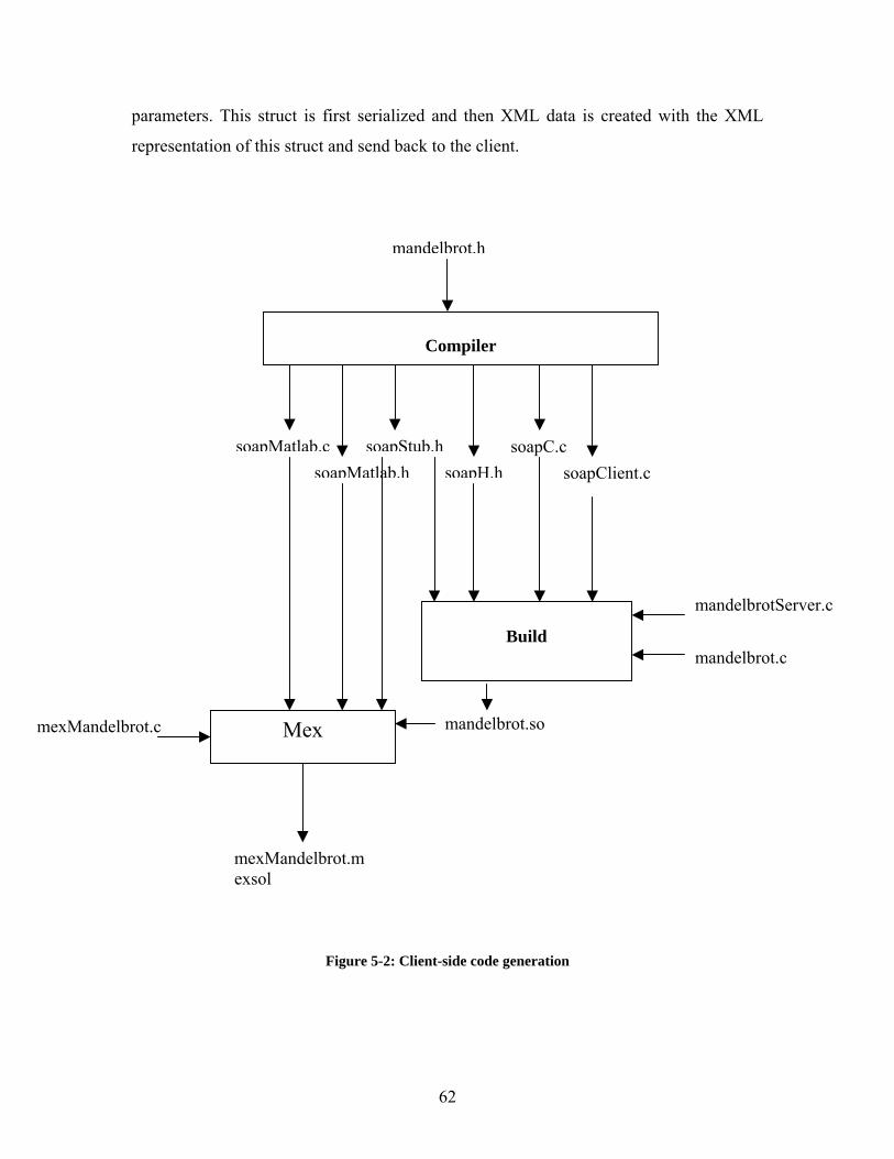
parameters. This struct is first serialized and then XML data is created with the XML
representation of this struct and send back to the client.
ch
mexMandelbrot.c Mex
r
mexMandelbrot.mexsol
Figure 5-2: Cli
Compile
soapC.c
soapStub.h soapClient.cent
soapH.h
mandelbrot.h
soapMatlab.
soapMatlab.Build
mandelbrot.so
mandelbrotServer.c
mandelbrot.c
-side code generation
62

The modified gSOAP compiler generates two additional files for data conversions
between MATLAB and C. This takes place at the client side.
1. soapMatlab.h declares the MATLAB to C conversion of all data types and vice
versa.
2. soapMatlab.c contains the definitions for the conversion routines of all data types
between C and MATLAB.
3. soapClient.c creates the XML output with the header and the XML representation
of the structure with the function’s parameters. When invoking a remote service
operation, the XML request is send to the server and the client then waits for the
response. The response arrives in the form of a result struct in XML, which is
automatically deserialized into a C struct.
Execution
Client Side Server Side
gSOAP serializer XML data
TCP/IP
MEX Remote
Application
MATLAB
User
Figure 5-3: Execution
63

MATLAB is integrated with gSOAP, which makes use of XML for data transfer. The
user invokes MATLAB on a local machine through a MEX-file. The MEX-file is
interfaced with a gSOAP runtime library, which exchanges XML messages with a remote
application. The user sends a request to a remote application, which processes it and
sends a response. The data returned from the application is then displayed in MATLAB.
The invocation of C from MATLAB requires data to be marshaled between the two
languages. This means that all data types in C should be mapped to corresponding data
types in MATLAB. The next section explains this in detail.
5.3 Mapping of C data types to MATLAB data types.
The compiler converts the following data types from MATLAB to C and vice versa:
• Basic data types - char, short, int, long, long long, float, double, unsigned char ,
unsigned short, unsigned int , unsigned long, unsigned long long,
• Pointers – Pointers to all the above specified basic data types to any level of
indirection are supported by the compiler,
• Structures, and
• Arrays (single, multi – dimensional and sparse arrays).
These conversion routines are generated by the modified gSOAP stub and skeleton
compiler. The implementation of the conversion routines as generated by the compiler is
discussed in the next section.
By default, encoding of the primitive types will take place as per SOAP encoding style.
The encoding can be changed to any XML schema type (XSD type) with an optional
namespace prefix by using a typedef in the header file input to the gSOAP stub and
skeleton compiler.
64

The serialization of a pointer to a data type amounts to the serialization of the data type in
SOAP and the SOAP encoded representation of a pointer to the data type is
indistinguishable from the encoded representation of the data type pointed to.
A struct data type is encoded as a SOAP compound data type such that the struct name
forms the data type's element name and schema type and the fields of the struct are the
data type's accessors.
Fixed size arrays are encoded as per SOAP 1.1 one-dimensional array types. Multi-
dimensional fixed size arrays are encoded by gSOAP as nested one-dimensional arrays in
SOAP. Encoding of fixed size arrays supports partially transmitted and sparse array
SOAP formats. Arrays in gSOAP are declared as structures, which contain the array
elements and the size. It is declared as given below-
struct some_name
{
Type *__ptr; // pointer to array
int __size; // number of elements pointed to
[[static const] int __offset [= ...];] // optional SOAP 1.1 array offset
... // anything that follows here will be ignored
};
The base64Binary XML schema type is a special form of dynamic array declared with a
pointer (__ptr) to an unsigned char array. For example using a struct:
struct xsd__base64Binary { unsigned char *__ptr; int __size; };
When compiled by the gSOAP stub and skeleton compiler, this header file specification
will generate base64Binary serializers and deserializers.
65

Implementation
The files soapMatlab.c and soapMatlab.h shown in Figure 5-2 are generated on
compilation. These files contain the conversion routines for all data types in the header
files passed as an argument to the compiler.
For example for the data type double, the following functions are generated
mxArray* c_to_mx_double(double );
void mx_to_c_double(const mxArray*,double *);
Both C to MATLAB (c_to_mx) and MATLAB to C (mx_to_c) functions are generated
for all the data types specified in the header file, which include basic data types, pointers,
structure and arrays. It is possible that these functions call other conversion functions. For
example, the function to convert MATLAB to C for pointer to doubles will call function
for MATLAB to C conversion for doubles. The conversion function generated for a struct
also calls the conversion functions for the struct’s data fields.
As an example we consider the data type ‘double’. The following functions
c_to_mx_double and mx_to_c_double are generated for doubles. The functions
c_to_mx_PointerTodouble and mx_to_c_PointerTodouble call functions
c_to_mx_double and mx_to_c_double respectively, passing the de-referenced pointer.
To invoke these methods in MATLAB, the functions generated by the compiler can be
used from a Mex-file. For ex. In the file mexMandelbrot.c, a call to the function
c_to_mx_ArrayOfDouble has been made, as
plhs[0] = c_to_mx_ArrayOfDouble(s) ;
66

The gSOAP compiler can convert sparse matrices in MATLAB to their C representation
and vice-versa. Besides this, gSOAP also has its internal sparse matrix representations.
Additional specialized data representations can be introduced to represent sparse
matrices. In order to do this, the user has to write custom serializers and deserializers. To
specify a type with a custom serializer, we declare it with the identifiers “extern typedef”
in the .h file for the gSOAP compiler.
67
CHAPTER 6
APPLICATIONS
In this chapter we demonstrate two applications of the tools we developed for Web
services computing with MATLAB. The first application was developed as a “proof of
concept” demonstration. The second application was developed for the visualization of
weather forecast data, where the data is produced by the HIRLAM weather forecast
system [47]. The HIRLAM weather forecasts data is served on demand to the MATLAB
client application by a server application we developed in C for this particular
demonstration.
In Section 6.1 we discuss about the visualization of the Mandelbrot set. The specialty
about the Mandelbrot set is that its boundary exhibits complicated structure at all length
scales from about 1 down as far as you wish (or as you computer will take you) to zero.
In other words, it is a fractal. And weather forecasting is discussed in section 6.2. This
system is a very complex system. The section explains its interface with MATLAB.
Visualizing the Mandelbrot Set
The Mandelbrot set, named after Benoit Mandelbrot, is a fractal. Fractals are objects that
display self-similarity at various scales. Magnifying a fractal reveals small-scale details
68

similar to the large-scale characteristics. Although the Mandelbrot set is self-similar at
magnified scales, the small scale details are not identical to the whole. In fact, the
Mandelbrot set is infinitely complex. Yet the process of generating it is based on an
extremely simple equation involving complex numbers.
6.1.1 Graphing the Mandelbrot set
The Mandelbrot set is a set of complex numbers, so we graph it on the complex number
plane. However, first we have to find many numbers that are part of the set. To do this we
need a test that will determine if a given number is inside the set or outside the set. The
test is based on the equation Z = Z2 + C. C represents a constant number, meaning that it
does not change during the testing process. C is the number we are testing, the point on
the complex plane that will be plotted when testing is complete. Z starts out as zero, but it
changes as we repeatedly iterate this equation. With each iteration we create a new Z that
is equal to the old Z squared plus the constant C. So the number Z keeps changing
throughout the test.
This application was developed as a “proof of concept” to demonstrate the application of
our Web services tools for MATLAB. In this demonstration setup, we developed a Web
service application in C that calculates the Mandelbrot set upon request by a MATLAB
client. The Web service is independent of MATLAB, and was written in C for
performance considerations. The service runs as a stand-alone HTTP deamon on a socket
port. It computes the fractal data set for visualization in MATLAB, where the data set is
produced upon request from the MATLAB script that is used to interactively visualize
the data. The fractal data is serialized in XML as two-dimensional SOAP-encoded arrays
of double floating point values. The server is developed with gSOAP from a C header file
specification.
struct ArrayOfDouble {
double *__ptr; int __size[2];
};
69
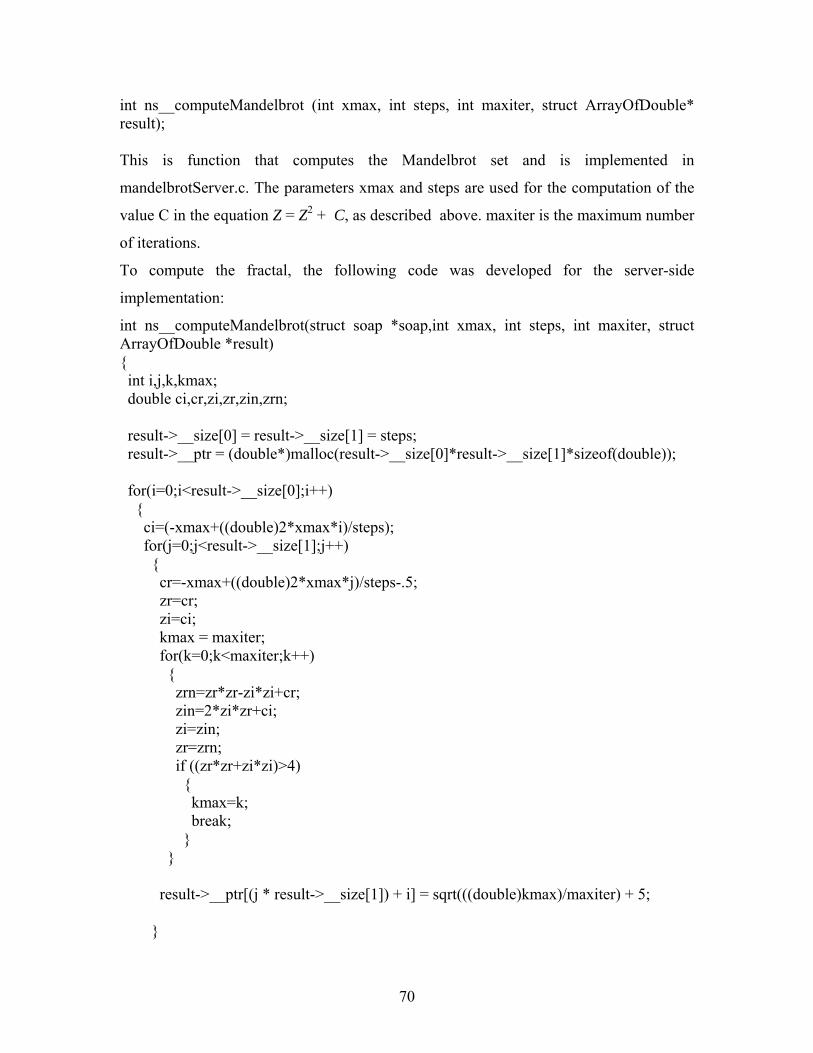
int ns__computeMandelbrot (int xmax, int steps, int maxiter, struct ArrayOfDouble* result); This is function that computes the Mandelbrot set and is implemented in
mandelbrotServer.c. The parameters xmax and steps are used for the computation of the
value C in the equation Z = Z2 + C, as described above. maxiter is the maximum number
of iterations.
To compute the fractal, the following code was developed for the server-side
implementation:
int ns__computeMandelbrot(struct soap *soap,int xmax, int steps, int maxiter, struct ArrayOfDouble *result) { int i,j,k,kmax; double ci,cr,zi,zr,zin,zrn; result->__size[0] = result->__size[1] = steps; result->__ptr = (double*)malloc(result->__size[0]*result->__size[1]*sizeof(double)); for(i=0;i<result->__size[0];i++) { ci=(-xmax+((double)2*xmax*i)/steps); for(j=0;j<result->__size[1];j++) { cr=-xmax+((double)2*xmax*j)/steps-.5; zr=cr; zi=ci; kmax = maxiter; for(k=0;k<maxiter;k++) { zrn=zr*zr-zi*zi+cr; zin=2*zi*zr+ci; zi=zin; zr=zrn; if ((zr*zr+zi*zi)>4) { kmax=k; break; } } result->__ptr[(j * result->__size[1]) + i] = sqrt(((double)kmax)/maxiter) + 5; }
70

} return SOAP_OK; } The image generated is given in Figure 6-1.
Figure 6-1: Mandelbrot Set
The server code is invoked from the following MEX-file:
void mexFunction( int nlhs, mxArray *plhs[], int nrhs, const mxArray *prhs[] ) { struct ArrayOfDouble s; int xmax = (int)mxGetScalar(prhs[0]); int steps = (int)mxGetScalar(prhs[1]); int maxiter = (int)mxGetScalar(prhs[2]); computeMandelbrot(xmax,steps,maxiter,&s); plhs[0] = c_to_mx_ArrayOfDouble(s);
71

} This MEX-file, gets the values of xmax, steps and maxiter, and calls the function
computeMandelbrot. The last parameter is the result of the computation and is passed
again to MATLAB as plhs[0].
To invoke the service, the following MATLAB code was written: xmax=2; steps=200; maxiter=32; X=[-xmax:2*xmax/(steps-1):xmax]; Y=[-xmax:2*xmax/(steps-1):xmax]; Z=mexMandelbrot(xmax,steps,maxiter); mesh(X,Y,Z); The first three statements initialize value for xmax, steps and maxiter. X, Y and Z are row
vectors. The vectors X and Y have values ranging from –xmax to xmax in steps of
2*xmax/(steps-1). The vector Z is a two dimensional vector returned by the MEX
function mexMandelbrot. The function mesh is used to plot the Mandelbrot set.
mesh(X,Y,Z) draws a wireframe mesh with color determined by Z so color is
proportional to surface height. For the vectors X and Y, if length(X) = n and length(Y)
= m, where [m,n] = size(Z), then (X(j),Y(i),Z(i,j)) are the intersections of the
wireframe grid lines; X and Y correspond to the columns and rows of Z, respectively.
6.1.2 Generating the MATLAB Interface
The code generated using gSOAP compiler provides the interface for the MATLAB
script. The files soapMatlab.h and soapMatlab.c contains conversion functions between
MATLAB and C. These conversion routines are for all the data types specified in the
header file passed as an argument to the gSOAP compiler. In this example the header file
mandelbrot.h contains the following declarations:
struct ArrayOfDouble{ double *__ptr; int __size[2];};
72

int ns__computeMandelbrot(int xmax, int steps, int maxiter, struct ArrayOfDouble *result); The files soapMatlab.h and soapMatlab.c have the following conversion routines for the
data types specified in the header file mandelbrot.h:
mxArray* c_to_mx_ArrayOfDouble(struct ArrayOfDouble ); void mx_to_c_ArrayOfDouble(const mxArray*, struct ArrayOfDouble *); mxArray* c_to_mx_int(int ); void mx_to_c_int(const mxArray*,int *); mxArray* c_to_mx_double(double ); void mx_to_c_double(const mxArray*,double *); mxArray* c_to_mx_PointerToArrayOfDouble(struct ArrayOfDouble *); void mx_to_c_PointerToArrayOfDouble(const mxArray*,struct ArrayOfDouble **); mxArray* c_to_mx_PointerTodouble(double *); void mx_to_c_PointerTodouble(const mxArray*,double **); These functions are used in the MEX-file mexMandelbrot.c. This is the file which is
invoked though MATLAB. The function mexFunction is the entry point to this file.
void mexFunction( int nlhs, mxArray *plhs[], int nrhs, const mxArray *prhs[] ) { . . int xmax = (int)mxGetScalar(prhs[0]); int steps = (int)mxGetScalar(prhs[1]); int maxiter = (int)mxGetScalar(prhs[2]); computeMandelbrot(xmax,steps,maxiter,&s); plhs[0] = c_to_mx_ArrayOfDouble(s); } The function computeMandelbrot is a function in mandelbrot.c and is defined as follows: void computeMandelbrot(int xmax, int steps, int maxiter, struct ArrayOfDouble *result) { int i; struct soap soap;
73

soap_init(&soap); fprintf(stderr,"in calc.c xmax=%d steps=%d maxiter=%d\n",xmax,steps,maxiter); soap_call_ns__computeMandelbrot(&soap, server, "",xmax, steps, maxiter,result);
.
.
. } A soap call is generated to the server through soap_call_ns__computeMandelbrot, which
invokes the function ns__computeMandelbrot in mandelbrotServer.c. The array “result”
contains the vector to be displayed. This vector is passed all the way from this file to the
MEX-file and further to the MATLAB code which initiates the call, where it is then
displayed with the mesh function.
6.2 Weather Forecasting
This application was developed to demonstrate the use of MATLAB to visualize large-
scale data sets produced by weather forecast systems. A server application was developed
in C to collect the data and send it to a MATLAB client application for visualization on
demand.
Weather forecast is widely used in many areas. It can be visualized and also manipulated
by MATLAB. Weather forecast data can have different formats for storage, depending on
the use. By developing a Web services interface, the data format does not matter, because
the data will be exchanged in standardized XML representation using multi-dimensional
SOAP-encoded (sparse) arrays. The advantage is that using XML as the lingua franca for
numerical data reduces the conversion complexity.
Another benefit of Web services is platform-independence. Data sources and sinks can be
developed in different languages, like FORTRAN, C, C++, etc. Using Web services tools
for these languages reduced the complexity of developing data communications between
74

these applications. For example, with gSOAP for C and C++ the data can be easily
serialized and de-serialized in XML.
6.2.1 Climate and Weather Forecast Models.
Climate and weather forecast models contain atmospheric models that can be
characterized by two main computational components: the dynamics, which is primarily
concerned with the fluid dynamics of the atmosphere and the physics, which is primarily
concerned with the computation of physical parameterizations. The dynamics and physics
operate on three-dimensional grids.
An example of climate and weather forecast systems with this structure is: the HIRLAM
numerical weather forecast system developed by the HIRLAM project group.
6.2.1.1 The HIRLAM System
The HIRLAM (High Resolution Limited Area Model) system is a production code
written in Fortran 77 developed by the HIRLAM-project group, a cooperative project of
Denmark, Finland, Iceland, Ireland, the Netherlands, Norway, Spain and Sweden. The
HIRLAM system comprises a so-called “limited area model” that encompasses a local
part of the globe which is logically rectangular of shape, as in figure 6-2. In the figure the
HIRLAM output is visualized using Vis-5D.
6.2.1.2 The HIRLAM Forecast Model
The HIRLAM weather forecast system contains five prognostic variables: two horizontal
wind components, temperature, specific humidity, and surface pressure. These variables
are defined on a spherical horizontal coordinate system. The vertical coordinate is a
hybrid coordinate between pressure and terrain following coordinates. All model
parameters are kept in memory; three-dimensional wind, temperature, liquid water, and
water vapor fields, and a two-dimensional surface pressure field.
75

The core of the HIRLAM system is provided by the so-called dynamics and the physics
routines.
Graphing the Weather Forecast Model
The server generates the weather forecast data. The code for the server side
implementation is given below:
int ns__getPressure(struct soap *soap, struct array2D *ppsz) { r2d(fd, "ppsz ", klon, klat, ppsz); r2d(fd, "pdpsdt", klon, klat, &pdpsdt); return SOAP_OK; } int ns__getData(struct soap *soap, struct data *d) { int i; d->puz = (struct array3D *)malloc(sizeof(struct array3D)); d->pvz = (struct array3D *)malloc(sizeof(struct array3D)); d->ptz = (struct array3D *)malloc(sizeof(struct array3D)); for (i = 0; i < klev; ++i) { r3d(fd, "puz ", klon, klat, klev, i, d->puz); r3d(fd, "pvz ", klon, klat, klev, i, d->pvz); r3d(fd, "ptz ", klon, klat, klev, i, d->ptz); r3d(fd, "pqz ", klon, klat, klev, i, &pqz); r3d(fd, "psz ", klon, klat, klev, i, &psz); r3d(fd, "pdudt ", klon, klat, klev, i, &pdudt); r3d(fd, "pdvdt ", klon, klat, klev, i, &pdvdt); r3d(fd, "pdtdt ", klon, klat, klev, i, &pdtdt); r3d(fd, "pdqdt ", klon, klat, klev, i, &pdqdt); r3d(fd, "pdsdt ", klon, klat, klev, i, &pdsdt); r3d(fd, "pgradx", klon, klat, klev, i, &pgradx); r3d(fd, "pgrady", klon, klat, klev, i, &pgrady); } return SOAP_OK; }
The argument ppsz in the function ns__getPressure is a two dimensional array of type
‘struct array2D’ which contains the pressure. The function ns__getData is used to
compute the wind velocity and temperature. The argument ‘struct data *d’, contains the
velocity and temperature. Both these structures are declared in a header file as shown
76

below. This header file is passed as an argument to the gSOAP compiler when it is
invoked.
struct array2D { double *__ptr; int __size[2]; }; struct array3D { double *__ptr; int __size[3]; }; struct data { struct array3D *puz; struct array3D *pvz; struct array3D *ptz; }; int ns__getPressure(struct array2D *ppsz); int ns__getData(struct data *d); The server code is invoked from the following MEX-file:
void mexFunction( int nlhs, mxArray *plhs[], int nrhs, const mxArray *prhs[] ) { struct array2D p; struct data d; getPressure(&p); plhs[0] = c_to_mx_array2D(p); getData(&d); plhs[1] = c_to_mx_array3D(*(d.puz)); plhs[2] = c_to_mx_array3D(*(d.pvz)); plhs[3] = c_to_mx_array3D(*(d.ptz)); } In this MEX-file, a call is made to the function getPressure. Pressure is stored in a two
dimensional vector, p, which is then converted to a MATLAB array plhs[0]. Similarly,
getData populates the structure ‘d’, with the components of velocity in the x and y
direction and the temperature. These are contained in the fields puz, pvz and ptz
respectively.
77

6.2.3 Invoking the MEX-File
Invoke the MEX-file version of weather forecast from the MATLAB interpreter as
• [P,U,V,D] = mexWeather; • contour(P,15);
• for i=1:16 • imagesc(D(:,:,i)); • end
• [x,y] = meshgrid(1:1:50,1:1:50); • z = ones(50,50); • w = zeros(50,50); • scale = 8; • hold on
• for i=1:16 • quiver3(x,y,z*i,U(:,:,i),V(:,:,i),w,scale); • end
• view([70 18])
MATLAB runs the MEX-file. The file MEX call mexWeather, returns four vectors P, U,
V and T, all of which contain vectors used in weather forecast. The vector P contains
pressure. The function contour displays isolines of pressure matrix P. The image
generated is shown in Figure 6-2.
78
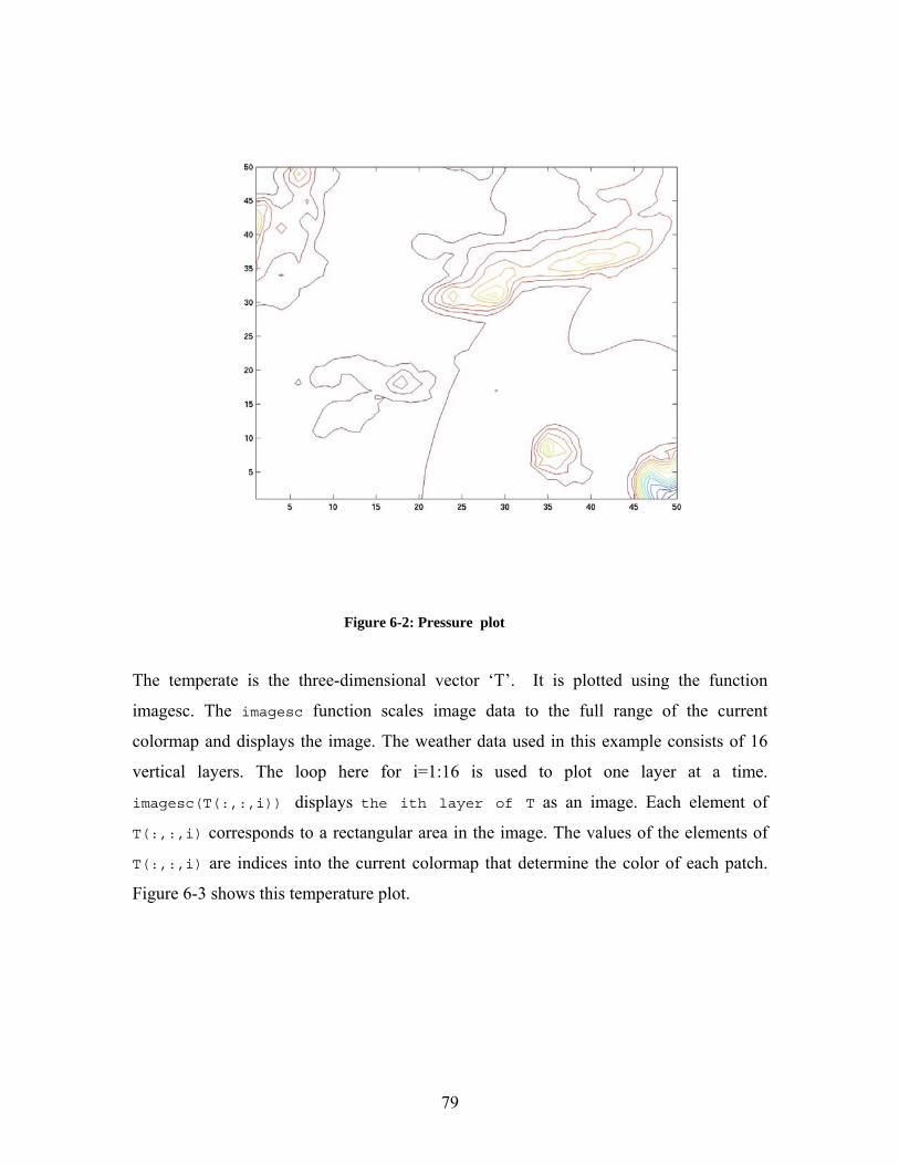
Figure 6-2: Pressure plot
The temperate is the three-dimensional vector ‘T’. It is plotted using the function
imagesc. The imagesc function scales image data to the full range of the current
colormap and displays the image. The weather data used in this example consists of 16
vertical layers. The loop here for i=1:16 is used to plot one layer at a time.
imagesc(T(:,:,i)) displays the ith layer of T as an image. Each element of
T(:,:,i) corresponds to a rectangular area in the image. The values of the elements of
T(:,:,i) are indices into the current colormap that determine the color of each patch.
Figure 6-3 shows this temperature plot.
79
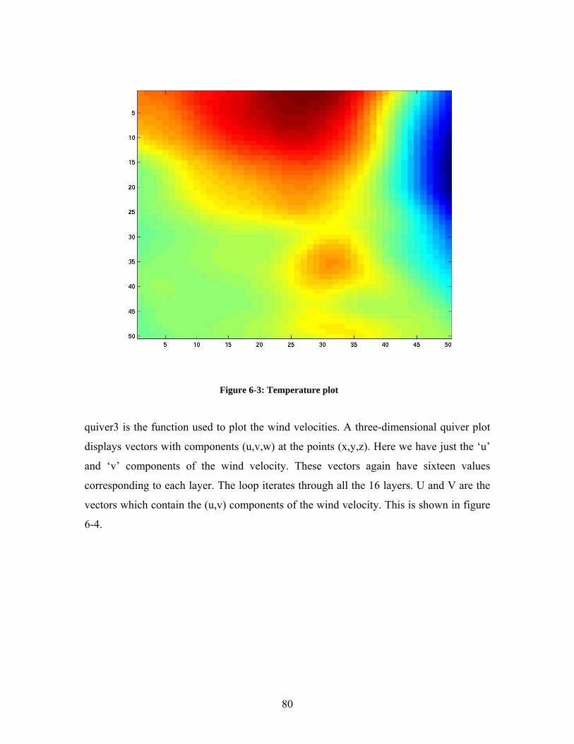
Figure 6-3: Temperature plot
quiver3 is the function used to plot the wind velocities. A three-dimensional quiver plot
displays vectors with components (u,v,w) at the points (x,y,z). Here we have just the ‘u’
and ‘v’ components of the wind velocity. These vectors again have sixteen values
corresponding to each layer. The loop iterates through all the 16 layers. U and V are the
vectors which contain the (u,v) components of the wind velocity. This is shown in figure
6-4.
80
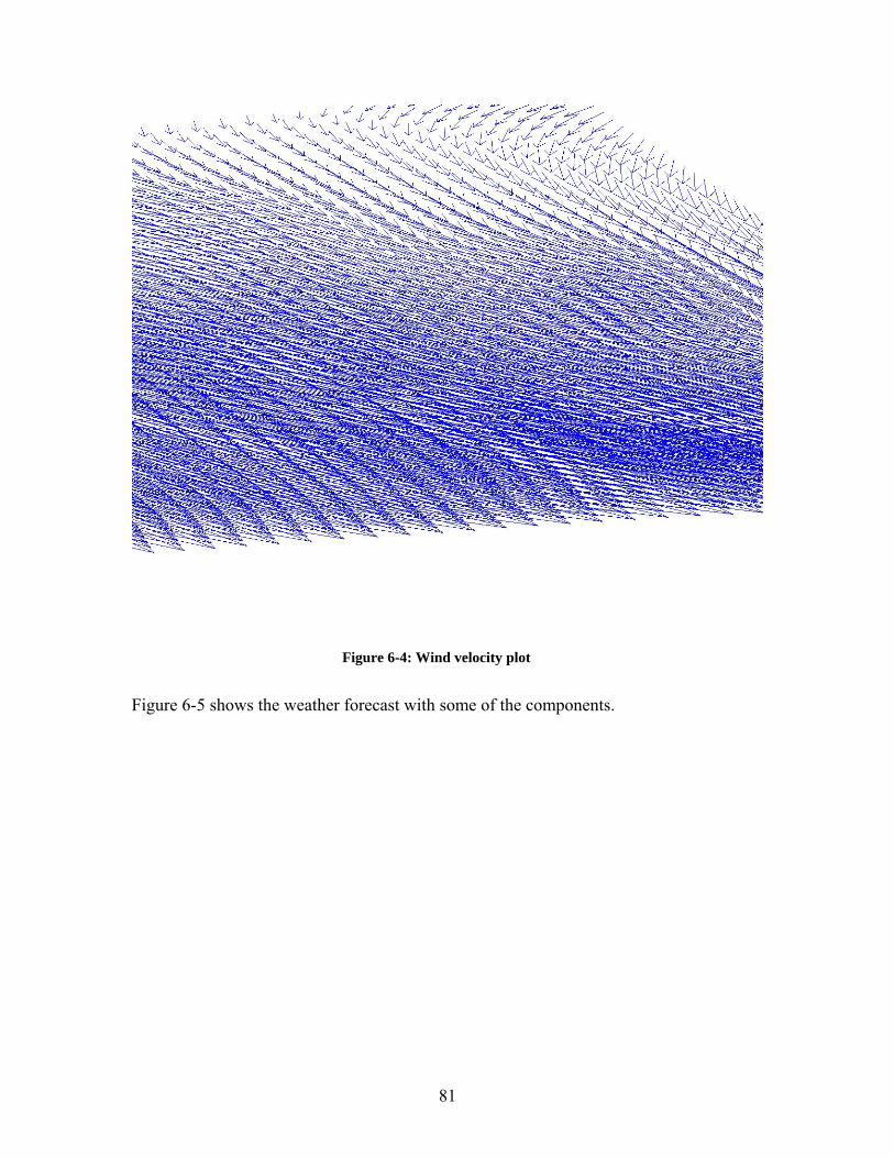
Figure 6-4: Wind velocity plot
Figure 6-5 shows the weather forecast with some of the components.
81
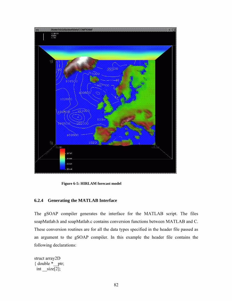
Figure 6-5: HIRLAM forecast model
6.2.4 Generating the MATLAB Interface
The gSOAP compiler generates the interface for the MATLAB script. The files
soapMatlab.h and soapMatlab.c contains conversion functions between MATLAB and C.
These conversion routines are for all the data types specified in the header file passed as
an argument to the gSOAP compiler. In this example the header file contains the
following declarations:
struct array2D { double *__ptr; int __size[2];
82

}; struct array3D { double *__ptr; int __size[3]; }; struct data { struct array3D *puz; struct array3D *pvz; struct array3D *ptz; }; int ns__getPressure(struct array2D *ppsz); int ns__getData(struct data *d); The files soapMatlab.h and soapMatlab.c have the following conversion routines for the
data types specified in the header file above:
mxArray* c_to_mx_int(int ); void mx_to_c_int(const mxArray*,int *); mxArray* c_to_mx_double(double ); void mx_to_c_double(const mxArray*,double *); mxArray* c_to_mx_data(struct data ); void mx_to_c_data(const mxArray*, struct data *); mxArray* c_to_mx_array3D(struct array3D ); void mx_to_c_array3D(const mxArray*, struct array3D *); mxArray* c_to_mx_array2D(struct array2D ); void mx_to_c_array2D(const mxArray*, struct array2D *); mxArray* c_to_mx_PointerTodata(struct data *); void mx_to_c_PointerTodata(const mxArray*,struct data **); mxArray* c_to_mx_PointerToarray2D(struct array2D *); void mx_to_c_PointerToarray2D(const mxArray*,struct array2D **); mxArray* c_to_mx_PointerToarray3D(struct array3D *); void mx_to_c_PointerToarray3D(const mxArray*,struct array3D **); mxArray* c_to_mx_PointerTodouble(double *); void mx_to_c_PointerTodouble(const mxArray*,double **);
83
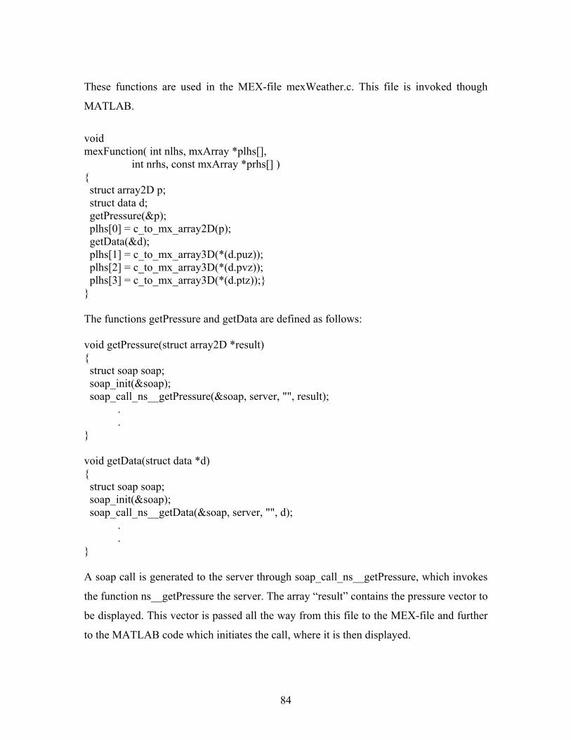
These functions are used in the MEX-file mexWeather.c. This file is invoked though
MATLAB.
void mexFunction( int nlhs, mxArray *plhs[], int nrhs, const mxArray *prhs[] ) { struct array2D p; struct data d; getPressure(&p); plhs[0] = c_to_mx_array2D(p); getData(&d); plhs[1] = c_to_mx_array3D(*(d.puz)); plhs[2] = c_to_mx_array3D(*(d.pvz)); plhs[3] = c_to_mx_array3D(*(d.ptz));} } The functions getPressure and getData are defined as follows: void getPressure(struct array2D *result) { struct soap soap; soap_init(&soap); soap_call_ns__getPressure(&soap, server, "", result); . . } void getData(struct data *d) { struct soap soap; soap_init(&soap); soap_call_ns__getData(&soap, server, "", d); . . } A soap call is generated to the server through soap_call_ns__getPressure, which invokes
the function ns__getPressure the server. The array “result” contains the pressure vector to
be displayed. This vector is passed all the way from this file to the MEX-file and further
to the MATLAB code which initiates the call, where it is then displayed.
84

Similarly, soap_call_ns__getData invokes the function ns__getData which returns the
wind velocity and temperature.
85

CONCLUSIONS
In this thesis we have attempted to integrate MATLAB with gSOAP for the visualization
of scientific computing and to demonstrate the support for representing and exchanging
sparse matrices in this approach. The gSOAP web services toolkit is a platform-
independent development environment for C and C++. This makes it possible to make
use of MATLAB over the web. Using gSOAP we can now access a remote processor for
computations, which need not have MATLAB installed on it.
MATLAB is one of the most popular applications used for visualizing of voluminous
data used in applications like scientific computing. Hence the integration of MATLAB
with web services makes it suitable for applications like atmospheric modeling, climate
modeling and geographic modeling.
Applications that do not use the Web, also benefit from this integration, because the
performance of MATLAB can be improved by making use of C. This can be seen in the
mandelbrot set example. Here we use a MEX file, which invokes gSOAP as compared to
a MATLAB implementation. The compiler promotes the use of MEX files as the
conversion of data between MATLAB and gSOAP is now automated.
86

There are a number of Grid computing applications that can make use of our approach,
for example Grid applications for numerical simulations that handle large numerical data
sets.
The current implementation converts MATLAB data types to C, and uses the
serialization and de-serialization routines of the converted C data-types. Another
approach could be to generate serialization and de-serialization routines for the
MATLAB data types directly instead of generating routines for intermediate conversions
to C data.
Defining more schemas for sparse representations should enhance the usability of this
approach. There are many types of sparse representations. The modified gSOAP compiler
build for this project currently supports only one of these representations. In addition,
automatic conversion of sparse matrix representations to a generic SOAP encoded sparse
array is preferable for those applications that do not support sparse matrix layouts but do
support the SOAP encoded sparse matrix format. The enables interoperability between
applications that support sparse representations and those that do not. The SOAP encoded
sparse array format reduces storage and communication costs.
Currently the base64 binary data exchange of dense matrix data in our approach assumes
IEEE754 floating point formats are used. When data is exchanged in a different floating
point format, the sender or receiver must check for the internal representation and convert
the format when appropriate.
87

REFERENCES
[1] R. van Engelen and K. Gallivan. The gSOAP toolkit for web services and peer-to-peer computing networks. In 2ndIEEE International Symposium on Cluster Computing andthe Grid, 2002. [2] Aart J. C. Bik Compiler Support for Sparse Matrix Computations. [3] S. Kamal Abdali and David S Wise. Experiments with quadtree representation of matrices. In P. Gianni, editor, Lecture Notes in Computer Science, No. 358, pages 96-108. Springer-Verlag,1988. [4] R.C. Agarwal, F.G. Gustavson, and M.Zubair. A high performance algorithm using pre-processing for the sparse vector matrix multiplication. In Proceedings of the International Conference on Supercomputing, pages 32-42,1992. [5] F.L. Alvarado. A note on sorting sparse matrices. In Proceedings of IEEE, volume 67, pages 1362-1263,1979. [6] Edward Anderson and Youcef Saad. Solving Sparse triangular linear systems on parallel computers. International Journal of high speed computing, 1(6):73-95,1989. [7] Thomas F. Coleman. Large sparse numerical optimization. In G. Goos and J.Hartmanis, editors, Lecture Notes in Computer Science, No. 165. Springer-Verlag, 1984. [8] A.R. Curtis and J.K. Reid. The solution of large sparse unsymmetric systems of linear equations. Joournal Inst. Maths. Applics.,8:344-353,1971. [9] Iain S Duff. MA28 – a set of Fortran subroutines for sparse unsymmetric liners equations. Technical Report AERE R-8730(1980 revision), Department of Computer Science, Leiden University, 1980.
88

[10] Iain S. Duff. Data Structures, algorithm and software for sparse matrices. In David j. Evans, editor, Sparsity and its applications, pages 1-29. Cambridge University Press, 1985. [11] Iain S. Duff, A.M.Erisman, and J.K.Reid. Direct methods of sparse Matrices. Oxford Science Publications, Oxford, 1990. [12] Iain S. Duff and J.K. Reid. Some design features of a sparse matrix code. ACM Transactions on Mathematical Software, pages 18-35,1979. [13] Jocelyne Erhel and Brenard Philippe. Multiplication of a vector by a sparse matrix on super-computers. In M. Cosnard, M.H. Barton, and M. Vanneschi, editors, Parallel Processing, pages 181-187. Elsevier Science Publishers B.V., North-Holland, 1988. [14] Alan George and Joseph W.H. Liu. A note on fill or sparse matrices. SIAM J. Numer.Anal.,12:452-455,1975. [15] Alan George and Joseph W.H. Liu. The design of a user interface for a sparse matrix package. ACM Transactions and mathematical software,5:139-162, 1979. [16] Alan George and Joseph W.H. Liu. A fast implementation of the minimum degree algorithm using quotient graphs. ACM Transactions and mathematical software,6:337-358,1980. [17] Alan George and Joseph W.H. Liu. Computer solutions of large sparse positive definite systems. [18] Fred G. Gustavson. Some basic techniques for solving sparse systems of liner equations. In Donald J. Rose and Ralph A. Willoughby, editors, Sparse Matrices and their applications, pages 41-52. plenum Press, New York, 1972. [19] Fred G. Gustavson. Two fast algorithms for sparse matrices: Multiplication and permuted transportation. ACM Transactions and mathematical software,4:250-269,1978. [20] Donald Hearn and M. Pauline Baker. Computer Graphics. Prentice-Hall International,1986. [21] A. Jennings. A compact storage scheme for the solution of symmetric linear simultaneous equations. The Computer Journal, 9:281-285,1966. [22] A. Jennings and A. D. Tuff. A direct method for the solution of large sparse symmetric simultaneous equations. In J.K. Reid, editor, Large sparse sets of linear equations, pages 97-104. Academic Press,1971. [23] Donald E. knuth. The Art of computer Programming. Addison Wesley, reading, Massachusetts, 1968. Volume 1:Fundamental Algorithms.
89
[24] Vipin Kumar, Ananth Grama, Anshul Gupta, George Karypis. Introduction to parallel programming. The Benjamin/cunnings publishing company, redwood city, CA,1994. [25] Joseph W.H. Liu. A generalized envelope method for sparse factorization of rows. ACM Transactions on Mathematical Software,17:112-129,1991. [26] Thomas C Oppe and David R. Kincaid. The performance of ITPACK on vector computers for solving large sparse linear systems arising in sample oil reservoir simulation problems. Communications is Applied Numerical Methods,3(1):23-29,1987. [27] Ole ∅sterby and Zahari Zlatev, Direct methods for sparse matrices. In g. Goos and j. Hartmanis, editors, Lecture Notes in Computer Science,No. 157. Springer-Verlag, berlin, 1983. [28] Sergio Pissanetsky, sparse matrix technology, academic press, London, 1984. [29] William H. Press, Brian P. Flannery, Saul A. Teukolsky, and William T. Vetterling. Numerical Recipes. Cambridge University Press, Cambridge, 1986. [30] Youcef Saad. Krylov subspace methods on supercomputers. SIAM J. Sci. Stat. Comput., 10:1200-1232,1989. [31] Youcef Saad. SPARSKIT: a basic tool kit for sparse matrix computations. CSRD/RIACS,1990. [32] Youcef Saad and harry A.G. Wijshoff. Spark: A benchmark package for sparse computations. In proceedings of the international Conference on Supercomputing, pages 239-253, 1990. [33] Hanan Samet. Connected component labeling using quadtrees. Journal of the ACM, 28:487-501,1981. [34] Reginal P. Tewarson. Sorting and ordering sparse linear systems. In J.K. Reid, editor, Large Sparse Sets of Linear Equations, pages 151-167. Academic Press, 1971. [35] Reginal P. Tewrson. Sparse Matrices. Academic Press, New York, 1973. [36] M Veldhorst. An Analysis of Sparse Matrix Storage Schemes. PhD thesis, Mathematisch Centrum, Amsterdam, 1982. [37] Harry A.G. Wijshoff. Implementing sparse BLAS primitives on concurrent /vector [38] David S. Wise. Representating matrices as quadtrees for parallel processing. Information processing Letters, 20:195-199,1985.
90
[39] David S. Wise. Parallel decomposition of matrix inversion using quadtrees. In proceedings of the International Conference on Parallel Processing, pages 92-99,1986. [40] David S. Wise. Undulant block elimination and integer-preserving matrix inversion. Technical Report 418, computer Science Department, Indiana University, 1995. [41] David S. Wise and John Franco. Costs of quadtree representation of nondense matrices. Journal of Parallel and Distributed Computing, 9:282-296,1990. [42] Zahari Zlatev, Computational Methids for General Sparse Matrices. Kluwer, Dordrecht, 1991. [43] Robert W. Sebesta, Concepts of programming languages, fourth edition. [44] Robert A. van Engelen, Pushing the SOAP Envelope With Web Services for Scientific Computing. [45] Web Services Architecture, W3C Working Group Note 11 February 2004. [46] Web Services Architecture, W3C Working Draft 14 May 2003. [47] Robert A. van Engelen, CTADEL: A Generator of Efficient Numerical Codes. [48] http://www.w3.org/TR/ws-arch/ [49] http://www-106.ibm.com/developerworks/web/library/w-ovr/?dwzone=web#h0 [50] http://www.gotdotnet.com/team/XMLwebservices/gxa_overview.aspx [51] http://msdn.microsoft.com/library/default.asp?url=/library/en-us/dnanchor/html/WebServicesAnchor.asp [52] http://www.extreme.indiana.edu/xgws/papers/soap-hpdc2002/soap-hpdc2002.pdf [53] http://web.cs.mun.ca/courses/cs3731/Other/scientific-computing.pdf [54] http://www.vbip.com/books/1861005091/chapter_5091_04.asp [55] http://www.cafeconleche.org/books/xmljava/chapters/ix01.html [56] http://www.w3.org/OOP/ [57] http://weblogs.cs.cornell.edu/AllThingsDistributed/archives/000120.html [58] http://www.mathcs.emory.edu/conferences/pc2005/themes.html
91

[59] http://mercury.it.swin.edu.au/ctg/AWSA04/Papers/gray.pdf [60] http://www.mathworks.com/company/newsletters/news_notes/may03/profiler.html [61] http://www.students.tut.fi/%7Ewarp/MandScripts/ [62] http://time.er.usgs.gov/manpages/matlab/help/techdoc/apiref/mxgetir.html#106737 [63] http://www.mathworks.com/company/newsletters/news_notes/sum98/sum98activex.html [64] http://www.mathworks.com/company/newsletters/digest/nov02/earth_pt3.html [65] http://www.math.princeton.edu/~jmjohnso/teaching/202Bfall00/DiscHtEqn.html [66] http://www-2.cs.cmu.edu/~scandal/cacm/node9.html [67]http://www.ingenta.com/isis/searching/ExpandTOC/ingenta?issue=pubinfobike://sage/j348/2004/00000018/00000002&index=5 [68] www.me.pdx.edu/~gerry/ MATLAB/programming/performance.html [69] http://www.ddewey.net/mandelbrot/ [70] http://www.vbip.com/books/1861005091/chapter_contents.asp
92

BIOGRAPHICAL SKETCH
The author was born on 8th June 1976 in Mwanza, Tanzania. She has had the privilege of
seeking education at a number of places in India and abroad. She graduated from Shri
Govindram Saxeria Institute of Science and Technology (S.G.S.I.T.S), Indore with a
Bachelor’s Degree in Computer Science in the year 1999. She then decided to enrich her
knowledge by applying it, and thus worked for three years at Impetus Technologies,
Indore, India. She also had the opportunity to visit the United States, and worked at the
client site at Vantive, now taken over by PeopleSoft, in Santa Clara, California. This is
the time when she decided to pursue her Masters here in the United States. She has now
attained an M.S. degree from Florida State University from the Department of Computer
Science.
93