The Fatigue Damage Spectrum and Fatigue Damage Equivalent ... · Presented at the 79th Shock and...

Presented at the 79th

Shock and Vibration Symposium: October 26 – 30, 2008 Orlando Florida

1

Implementing the Fatigue Damage Spectrum and Fatigue

Damage Equivalent Vibration Testing

Scot I. McNeill, Ph.D.

Stress Engineering Services, Inc.

13800 Westfair East Drive

Houston, TX 77041

[email protected]

In this paper, a type of response spectra in which fatigue damage is the ordinate is reviewed.

Computation of this Fatigue Damage Spectrum (FDS) in both the time and frequency domains is

discussed. The method of Fatigue Damage Equivalent vibration Testing (FDET) is discussed

using the FDS as the measure of environment severity. Improvements in each technique over

previous work are introduced and the concepts are presented in a unified fashion. Efficient

computation of the various elements involved in the FDS and FDET is discussed and examples are

given.

INTRODUCTION

Various authors have introduced the concept of a Fatigue Damage Spectrum (FDS). The FDS is a type of response spectrum,

similar to the Shock Response Spectrum, except that the ordinate for this type of response spectrum is the fatigue damage

incurred in each single Degree Of Freedom (DOF) oscillator. The concept was introduced as a method to examine the

severity of frequency domain environments described by Acceleration Power Spectral Density (APSD) curves and time

duration [1]. Certain requirements on the acceleration environment are required for validity of this method. Most

importantly, the underlying process associated with the APSD must be a “strongly mixed” random process. In addition, the

APSD must be approximately uniform over the half power bandwidth of each oscillator. In [1] the FDS, named the Damage

Potential (DP), was proposed as a method used to evaluate the fatigue potential of electrodynamic and electrohydraulic

shakers as well as pneumatic hammer-driven repetitive shock shakers (at frequencies above 4 times the hammer rate). Since

the publishing of [1], the method has been used to evaluate the fatigue potential of different shakers [2].

It is apparent that the FDS can be computed in the time domain from a time history of the acceleration environment by cycle

counting and damage accumulation techniques. Reference [3] discusses the use of the FDS to compare test specifications to

measured environmental data. This reference illustrates the steps involved in computing FDS in the time domain and

frequency domain. In addition, the FDS of a specified environment is computed in the time domain and frequency domain

and the two FDS curves are shown to be equivalent.

The ability to compute the FDS in both the time and frequency domain and get equivalent results is the crux of the method of

Fatigue Damage Equivalent vibration Testing (FDET). In this method a Gaussian random test environment and duration is

derived such that it is fatigue equivalent to a non-stationary environment described by an acceleration time history. The time

history is normally obtained by direct measurement of the environment, such as placing accelerometers in a rocket payload

module. Roughly speaking, the FDS of the non-stationary time history environment is computed and then the Gaussian

random APSD curve and duration is derived which results in the same FDS. Though most of the theoretical results have

been published for some time, the concepts were first brought together in [4], and later in [5]. Commercial software

implementing this methodology has been developed recently, [6].

The purpose of this paper is to provide a unified theoretical framework for the FDS and FDET. Along the way improvements

are introduced such as accounting for the APSD shape in computation of the FDS in the frequency domain, using rainflow

cycles in computing the FDS in the time domain, and use of pseudo-velocity cycles (roughly proportional to stress cycles) in

the computation of the FDS in both frequency and time domain. Some other improvements in the FDET technique are

introduced, including estimation of overall test duration and a refinement technique that accounts for spectral shape in



2

deriving the APSD from the FDS. Efficient computation of the various elements involved in the FDS and FDET is discussed

and examples are given to illustrate the techniques.

FATIGUE DAMAGE SPECTRUM

In this section response spectra are briefly reviewed. Then the notion of the Fatigue Damage Spectrum is introduced.

Computation in the time domain and frequency domain is discussed.

(PEAK) RESPONSE SPECTRA

Response spectra have been used to characterize shock and vibration environments and compare their severity. Response

spectra consider the effect of an environment on a set of Single Degree Of Freedom (SDOF) oscillators. In general, a set of

SDOF oscillators is modeled with a range of natural frequencies (fn) and usually a single quality factor (Q). The response of

each oscillator to the vibration environment is computed. Some feature of the response (e.g. peak response) is computed and

plotted vs. natural frequency. The most well known type of response spectrum is the Shock Response Spectrum (SRS). The

SRS is the peak oscillator response to a transient time history of the shock environment. Usually, the SRS is computed in the

time domain by simulation of discrete time oscillator models [8]. A similar spectrum of peak oscillator absolute acceleration

to a Gaussian random environment, described by a PSD, is known as the Vibration Response Spectrum (VRS) [9]. The VRS

is computed in the frequency domain by integrating the oscillator’s frequency response to obtain the Root Mean Square

(RMS) response. The peak response for Gaussian random excitation can be approximated by multiplying the RMS response

by sqrt(2*ln(fn*T)). Here T is the environment duration and ln(·) is the natural logarithm. There are several responses of

interest for the SRS. Most often the absolute acceleration, relative displacement, and pseudo-velocity are computed. A

relative displacement SRS is presented as a plot of peak relative displacement on the ordinate vs. natural frequency on the

abscissa. The VRS can also be generalized to accommodate all the various ordinates (response types). Typically the

vibration environment is described by base-drive acceleration time history or APSD.

The response spectra discussed above are the curves that describe the peak response of a set of oscillators to a vibration

environment. One of the drawbacks of describing a vibration environment with the SRS is that the response spectra are not

associated with a unique base acceleration environment. (The transformation from base acceleration time history to SRS is

not uniquely invertible.) As a result, a less severe base acceleration may produce the same SRS as the original environment

from which the SRS was derived. Therefore if a shock test specification is described by an SRS, a more benign time history

may be used to test the component than was intended. Due to this problem, the SRS description of a shock environment is

typically supplemented with temporal information about the transient environment. This usually comes on the form of band

limited temporal moments. The ith temporal moment, mi(a), of time history f(t) about time a is given in Eq. (1). Usually the

energy, RMS duration and root energy amplitude are sufficient for supplementing the SRS specification [10]. These

quantities are obtained from the first three moments as shown in Table 1. Note that under the assumptions that the

acceleration environment is Gaussian random and the APSD is flat in the half power bandwidth, the VRS has a unique APSD

environment associated with it. In this case, the relationship between the APSD base acceleration and the (peak absolute

acceleration) VRS, for an oscillator with natural frequency fn, quality factor Q, and base APSD level at the natural frequency

Pa(fn), is simply given by the familiar Miles’ equation, Eq. (2).

dttfatam 2i

i

(1)

nannn fPfQ2

πT)2ln(fQ,fVRS

(2)

Table 1: Temporal Moments in Physical Units

Energy (E) E = m0(0)

Centroid (C) C = m1(0) / m0(0)

RMS Duration (D) D2 = m2(C) / E

Root Energy Amplitude (R) R2 = E / D



3

FATIGUE DAMAGE SPECTRUM (TIME DOMAIN)

While the SRS and the VRS are good measures of the potential of a base acceleration environment to induce peak response

on a structure, they lack information on the number of cycles the environment induces on the structure. To address this

deficiency, a response spectrum can be devised whose ordinate is a measure of the fatigue damage of each oscillator. This

kind of response spectrum is called the Fatigue Damage Spectrum (FDS). Calculation of the FDS in the time domain is

straightforward albeit computationally expensive.

Computation of the FDS in the time domain begins the same way as does the SRS. First the base acceleration time history

for the non-stationary environment is obtained and detrended. Then the pseudo-velocity time history response is computed

for each oscillator. Then, instead of finding the peak oscillator response, each response is then run through a rainflow fatigue

cycle counting routine to develop cycle spectra. Cumulative damage is then computed by combining Minor’s rule and the S-

N law, for each oscillator (assuming fatigue exponent, b). The oscillator damage can then be plotted vs. the oscillator natural

frequency. In the next few sections the governing equations and computational methods will be reviewed for each step of the

process below.

1. Obtain acceleration time histories describing the vibration environment, a(t). Detrend and up-sample if needed.

For each SDOF oscillator with natural frequency fn and quality factor Q:

2. Compute the pseudo-velocity response pv(t).

3. Count pseudo-velocity rainflow cycle spectra, n(PV)

4. Compute the oscillator cumulative damage using Minor’s rule and the S-N law (assuming fatigue exponent, b),

D(fn,Q,b).

5. Plot the oscillator cumulative damage D(fn,Q,b) on the ordinate vs. the oscillator natural frequency on the abscissa. The

spectrum D(fn,Q,b) is called the Fatigue Damage Spectrum.

OBTAINING ACCELERATION TIME HISTORY – DETRENDING

Time history acceleration environments can be obtained by placing accelerometers near the attachment locations of

components. If the mass of the component is large, it may be best to measure the environment with the component or a mass

simulator attached. It is almost always the case that steady state accelerations and low frequency transients are handled by

separate requirements, to which random vibration effects are added to derive design loads. Therefore it is desirable to

remove the rigid body and very low frequency transients from the time history. This can be done by a generic process called

detrending. There are many ways to remove the very low frequency trends from data: high pass digital filtering, Fourier or

Wavelet filtering, fitting and removing polynomials, etc. In this paper, data has been detrended by fitting piecewise spline

curves to the data to represent the trend. The trend can be removed by subtracting the fitted curve from the data, leaving only

the desirable data. This method has been found to be a robust method for different types of data and associated trends. This

is accomplished in MATLAB® by computing 20 or so moving average points and up-sampling to the data length by using the

interp1 command with the ‘spline’ option.

The time history may need to be up-sampled if the sampling rate is too low. More comments on the criteria and techniques

are in the next section.

COMPUTATION OF PSEUDO-VELOCITY OSCILLATOR RESPONSE

It has been shown that the pseudo-velocity is more closely related to stress than other response measures, such as absolute

acceleration [7, 11, 12, 13]. The relationship between pseudo-velocity and stress is roughly proportional. Therefore it is

imperative that cycles are counted on the pseudo-velocity response of each SDOF oscillator in order to produce a meaningful

FDS, since fatigue damage is related to stress cycles. The transfer function between base acceleration and pseudo-velocity is

given by Eq. (3), where ς is the damping ratio (ς = 1/2Q) and ωn is the circular natural frequency (2πfn). This transfer

function is simply that for relative displacement scaled to a velocity measure by multiplication with ωn.

A fast technique for computing the pseudo-velocity response is to convert to a discrete time filter model. The ramp-invariant

discrete time relative displacement model (scaled to pseudo-acceleration) has been published in [8] for use in SRS

computation. The pseudo-velocity model can be obtained by simply dividing by ωn. The result is given in Eq. (4), where Ts

is the sampling interval for the acceleration time history. This pseudo-velocity response samples of the filter model, pv(k),

to the base acceleration, a(k), is given in Eq. (5). Sample number can be converted to time by (t(k) = k*Ts). This type of

recursive formula is implemented in MATLAB® by using the filter command.



4

2

nn

2

n

ωsωζ2s

ωsH

(3)

2

2

ns

2

2

ns

2

2

22

ns2

ns

1

ns2

2

2

ns

0

2

210

ds

Tζω

2

nd

2

2

1

10

2

2

1

10

ζ1

S12ζC2ζ2ζωTE

ωT

1b

ζ1

S12ζ2E12ζωTC2

ωT

1b

ωTSζ1

12ζ1C2ζ

ωT

1b

Ea2C,a1,a

EsinKSEcosK,C,ωTK,eE

ζ1ωω

wherezazaa

zbzbbzH

~

sn

(4)

2kpva1kpva2kab1kabkabkpv 21210 (5)

It has been shown that due to the low pass effect of the ramp invariant method, if natural frequencies of greater than 17% of

the sampling frequency (fs = 1/Ts) are excited by the input acceleration, the peak accelerations could be 10% in error [14].

Therefore it is recommended that the sample rate be greater than 10 times the maximum frequency content in the acceleration

time history (fs ≥ 10*fmax). If the acceleration history is not sampled at a high enough rate, it can be resampled by up-

sampling (zero insertion), FIR filtering and down sampling. This can be done with upfirdn or resample functions in

MATLAB®. The additional computational expense of resampling and filtering an acceleration history of increased size can

be avoided by applying the low-pass compensating pre-filter of [14] to the acceleration time history before computing the

SDOF response. The pre-filter is given in Eq. (6). The pre-filter can be implemented in MATLAB® by using the filtfilt

command resulting in zero phase distortion of the acceleration history. This technique extends the sampling criteria to 4/5

the Nyquist frequency (fs ≥ 5/2*fmax). Since computation of the pseudo-velocity response is done for each oscillator natural

frequency, implementing this fast and accurate technique is highly desirable to save cpu time.

321

21

0.0659z0.8111z1.6296z1

0.8767z1.7533z0.8767zH

~

(6)

During computation of pseudo velocity response, it is important to compute cycles due to the oscillator decay after loading

ends. This can be done by zero-padding the acceleration history by a factor of (N*fs/fn), where N is the number of cycles to

compute after loading terminates.

RAINFLOW CYCLE COUNTING

As mentioned previously, fatigue damage on a structure requires a stress cycle count. Since pseudo-velocity is roughly

proportional to stress for many structures, a scale factor exists between stress, σ(t), and pseudo-velocity, pv(t), ( σ(t) =

k*pv(t) ). In general cycles are found within time histories by finding patterns that meet the definition for a specific type of

cycle. Many definitions of cycles exist: peak-valley, level crossing, range pair, rainflow, etc. [15]. The rainflow definition of

a cycle is the most related to structural damage because it is equivalent to closed hysteresis loops in a material stress-strain

plane. In [4, 16], a more simplified definition of a cycle was used that is valid for a narrow band signal. However it was

found that when the oscillator natural frequency is away from a spectral peak in the acceleration environment, the narrow

band assumptions are violated. This resulted in the narrow band cycle counter giving poor results compared to the rainflow

cycle counter, which is valid for wide band signals. This condition can happen often with non-stationary acceleration

environments. For example, if there is a low frequency bias due to gravity or rigid body acceleration, the narrow band



5

counter will fail to give accurate results. Typically, narrow band cycle counts on wide band data can over estimate damage

[17], however due to the definition of a cycle in [4], the counter was found to under predict damage for wide band response

since it will miss high amplitude cycles that occur over periods of time larger than the oscillator natural period.

There are many equivalent definitions of rainflow cycles [15]. For the results in this paper, the 4-point algorithm, [20], was

used to count rainflow cycles. Cycle counting algorithms begin with a sequence of extrema (peaks and valleys) of a time

history. The 4-point algorithm considers 4 consecutive extrema of the time history at a time (S1, S2, S3, S4). Three

consecutive ranges are formed by: Δ S1 = │S2 - S1│, Δ S2 = │S3 – S2│, Δ S3 = │S4 – S3│. If Δ S2 is less than or equal to its

adjacent ranges, it is counted as a cycle and its extremes are removed from the extrema sequence. The extrema that do not fit

this definition are left in the sequence residual and counted as half cycles. Further discussion of the algorithm is beyond the

scope of this paper. More information on counting techniques can be found in [15].

The counting routine was implemented in MATLAB® as an m-file. The routine can be implemented faster by writing the

routine in C or FORTRAN and creating a Matlab EXecutable (MEX) file. This was not attempted since the m-file run time

was reasonable. The counting technique results in values of cycle amplitude and cycle mean for each cycle counted in the

time history.

Both alternating stress (cycle amplitude) and mean stress (cycle mean) are important for damage. Mean stress becomes

significant in wide band response or in the presence of low frequency bias. Since the most common cumulative damage

relation (Minor’s rule) does not account for mean stress, the alternating and mean stress for each cycle can be used to convert

to a damage equivalent alternating stress (with no mean stress). Equation (7) contains a corrected alternating stress σa’,

computed from a Goodman Line. Here σa is the alternating (cyclic) stress amplitude, σm is the mean stress, and Sut is the

ultimate stress for the material. It can be seen that the correction becomes significant as σm approaches Sut.

In non-stationary vibration environments of vehicles, the largest component of mean stress comes from low frequency bias

due to rigid body motions. As mentioned previously, this is intentionally removed from the data by detrending. This leaves

mean stress due to wide band response. Wide band response will occur in SDOF response when there is significant energy

content of the acceleration environment away from the resonant frequency. Due to the SDOF frequency response magnitude

shape, this results in fairly small response of the oscillator. Therefore the mean stress σm should be small compared to the

ultimate stress Sut. As a result, the mean stress due to wide band response can be ignored without much loss of accuracy.

ut

m

aa

S

σ1

σσ'

(7)

The cycle count data can then be presented as a 2-D histogram of number of cycles vs. alternating (cyclic) amplitude, ni(PVi).

This is often called a cycle spectrum or counting distribution. Usually bins of varying amplitude range are assigned, and the

number of cycles falling in each bin’s range are assigned. In this paper 64 bins were created spanning the lowest cycle

amplitude to the highest cycle amplitude. It is often practical to rainflow filter the cycles so that the very small cycles are not

counted, since they are not significant for damage anyway. In this paper, cycles below 1% the peak cycle amplitude were

filtered out.

COMPUTING CUMULATIVE DAMAGE

Computing fatigue damage, D, from cycle spectra involves combining the Palgrem-Minor rule, Eq. (8), with the S-N relation,

Eq. (9). Here ni is the number of cycles with stress amplitude Si, Ni is the number of cycles with stress amplitude Si needed

to cause failure, c is a constant of proportionality and b is the fatigue exponent. Fatigue exponent ranges from 4 to 25. A

factor of b = 8 is commonly used for structural materials used in transportation. Constant c can be set to unit value since

proportionality does not affect the use of the FDS for environment comparison.

i i

i

N

nD (8)

b

ii cSN

(9)

Recall that a pseudo-velocity spectra, ni(PVi), is available, and that pseudo-velocity is roughly proportional to stress by

constant k. Therefore, the following damage equation is arrived at:



6

i

b

ii

b

.PVnc

kD (10)

Here ni is the number of cycles with pseudo-velocity amplitude PVi. Pseudo-velocity response, cycle count, and damage is

computed for each oscillator natural frequency to form the FDS, D(fn,Q,b).

FATIGUE DAMAGE SPECTRUM (FREQUENCY DOMAIN)

Computation of the FDS in the frequency domain is much less computationally intensive than computation in the time

domain, but requires more theoretical development. It is probably best to work backwards in the derivation as was done in

[1]. The goal is to compute the FDS, D(fn,Q,b), from an APSD of the acceleration environment. In order for the computation

to be valid it is assumed that the underlying process associated with the APSD must be a “strongly mixed” stationary random

process. In addition, the APSD must be approximately uniform over the half power bandwidth of each oscillator. A further

assumption is that damping is light (ς ≤ 0.1). Note that half power bandwidth is approximated by (Br = 2ςfn) for light

damping. In this case, the SDOF oscillator response will be narrow-band.

Derivation begins with the continuous form of the damage rule in Eq. (10) for a stationary signal, written in terms of stress

instead of pseudo-velocity [1]. In equation (11) p(S) is the Probability Density Function (PDF) of the stress maxima, T is the

total time of exposure to the stress environment and vm+ is the number of positive maxima per unit time in the stress history.

Note that for a narrow band lightly damped oscillator response, maxima occur every 1/fn seconds. So vm+ may be replaced

with fn. In addition, under the assumptions, the oscillator response will be nearly Gaussian regardless of the PDF of the

acceleration environment, and the PDF for the peaks will be nearly Rayleigh in form [18, 23]. Equation (12) shows the

Rayleigh distribution for the peaks. Here S is the stress value of the peaks and σs is the RMS of the stress time history.

0

bm dSSSpc

TvD (11)

2s

2

2σS

eσ

SSp

2

s

(12)

Solving Eq. (11) with Eq. (12) leads to Eq. (13), where Γ is the Gamma function. Note that in [16], different limits of

integration were chosen, resulting in more cumbersome expressions.

2

b1Γσ2

c

TfD

b

sn (13)

Recalling the relationship between pseudo-velocity and stress, Eq. (13) can be rewritten.

2

b1Γ2σk

c

TfD 2

b2

pv

bn (14)

The RMS pseudo-velocity oscillator response can be computed by exploiting Parseval’s theorem. First the square of the

frequency response magnitude is computed by multiplying the pseudo-velocity FRF square magnitude by the APSD. The

result is then integrated over all frequencies to compute the oscillator pseudo-velocity RMS, σpv, in terms of the APSD level,

Pa. The assumption that the APSD environment is relatively flat in the half power band width of each oscillator allows the

closed form approximation (similar to the Miles’ equation) to be used, Eq. (15). (The closed form solution assumes an

infinite flat, white noise APSD base drive acceleration.)

n

na

pvfπ8

QfPσ (15)

If the flatness assumption holds only weakly at some frequencies, the integration can be performed numerically to account

for the APSD shape, Eq. (16). Here fi is the ith frequency sample, ri = fi/fn is the ith normalized frequency, and Δfi is the

frequency spacing. Note that Eq. (15) is invertible allowing Pa(fn) to be solved, while Eq. (16) is not. This is important for

the FDET method.



7

N

1i

iia2

i22

i

2

npv ΔffP

Q

rr1

fπ2

1

σ (16)

RMS pseudo-velocity response is computed via Eq. (15) or Eq. (16) and damage is computed via Eq. (14) for each oscillator

natural frequency to form the FDS, D(fn,Q,b). Whichever equation is used, the APSD may have to be interpolated. In is

usually appropriate to logarithmically interpolate, such that interpolated values between two points will lie on a straight line

in a log-log plot. Interpolating the APSD at a frequency, fi, which lies between f1 and f2 with corresponding APSD levels A1

and A2 can be accomplished with the following equations, where N is the logarithmic slope and any base can be used for the

logarithm.

2N

n

i1i

1

2

1

2

f

fAA,

f

flog

A

Alog

N

(17)

Computation of the FDS in the frequency domain is quite simple, requiring only closed form equations or a simple numerical

integration scheme.

FATIGUE DAMAGE SPECTRUM (TIME & FREQUENCY DOMAIN EQUIVALENCE)

Since the FDS can be computed in the time domain for arbitrary acceleration histories and in the frequency domain for

stationary strongly mixed random data, it is natural to verify that the FDS of a stationary random signal computed in the time

domain and frequency domain are similar. In order to verify that the two methods produce similar results, an APSD

acceleration level was prescribed. An equivalent time history (time history with the prescribed APSD) was produced by

assuming that the phase angles associated with the spectrum (square root of APSD) are random and uniformly distributed

between –π and π radians. Generating the time history by inverse Fourier transform will then lead to an ergodic-stationary,

Gaussian, random time history that yields, exactly, the specified APSD [17]. Note that the APSD must be uniformly spaced

for most inverse Fourier transform algorithms (ifft in MATLAB®). The specified APSD level is given in Table 2. The APSD

specification and the equivalent time history are plotted in Figure 1. Note that a frequency resolution of 0.05 Hz was used to

interpolate the APSD specification and the interpolated APSD was zero padded with 100 zeros above 2000 Hz to increase the

time duration of the equivalent time history.

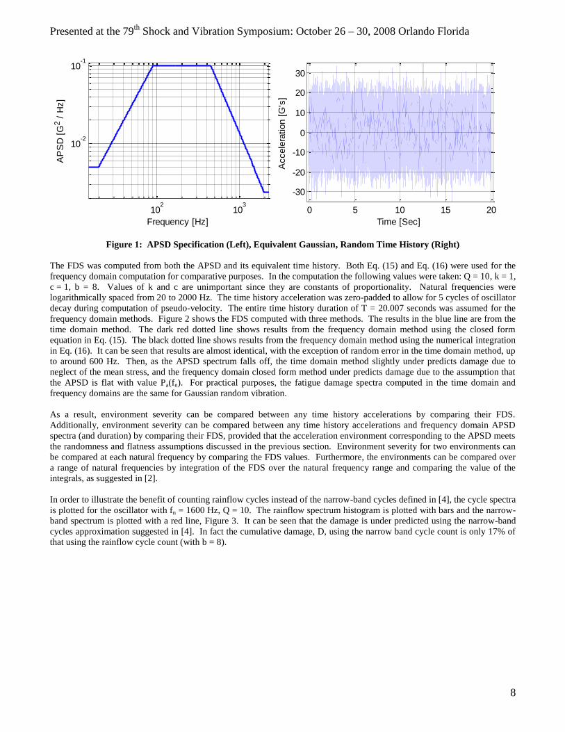
Table 2: APSD Specification

Frequency [Hz] APSD Specification

5 0.005 [G2/Hz]

20 0.005 [G2/Hz]

20-90 +6 dB/Octave

90-450 0.1 [G2/Hz]

450-2000 -7.5 dB/Octave

2000 0.0024 [G2/Hz]

2500 0.0024 [G2/Hz]



8

102

103

10-2

10-1

Frequency [Hz]

AP

SD

[G

2 /

Hz]

0 5 10 15 20

-30

-20

-10

0

10

20

30

Time [Sec]

Accele

ration [

G's

]

Figure 1: APSD Specification (Left), Equivalent Gaussian, Random Time History (Right)

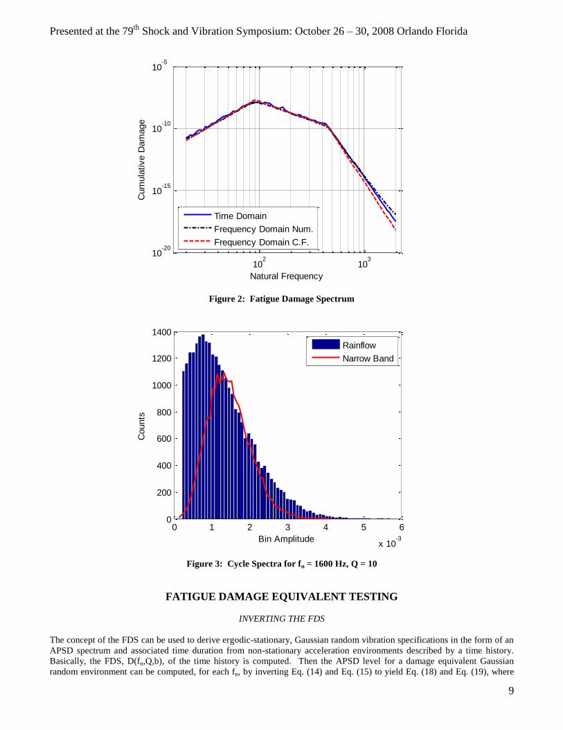
The FDS was computed from both the APSD and its equivalent time history. Both Eq. (15) and Eq. (16) were used for the

frequency domain computation for comparative purposes. In the computation the following values were taken: Q = 10, k = 1,

c = 1, b = 8. Values of k and c are unimportant since they are constants of proportionality. Natural frequencies were

logarithmically spaced from 20 to 2000 Hz. The time history acceleration was zero-padded to allow for 5 cycles of oscillator

decay during computation of pseudo-velocity. The entire time history duration of T = 20.007 seconds was assumed for the

frequency domain methods. Figure 2 shows the FDS computed with three methods. The results in the blue line are from the

time domain method. The dark red dotted line shows results from the frequency domain method using the closed form

equation in Eq. (15). The black dotted line shows results from the frequency domain method using the numerical integration

in Eq. (16). It can be seen that results are almost identical, with the exception of random error in the time domain method, up

to around 600 Hz. Then, as the APSD spectrum falls off, the time domain method slightly under predicts damage due to

neglect of the mean stress, and the frequency domain closed form method under predicts damage due to the assumption that

the APSD is flat with value Pa(fn). For practical purposes, the fatigue damage spectra computed in the time domain and

frequency domains are the same for Gaussian random vibration.

As a result, environment severity can be compared between any time history accelerations by comparing their FDS.

Additionally, environment severity can be compared between any time history accelerations and frequency domain APSD

spectra (and duration) by comparing their FDS, provided that the acceleration environment corresponding to the APSD meets

the randomness and flatness assumptions discussed in the previous section. Environment severity for two environments can

be compared at each natural frequency by comparing the FDS values. Furthermore, the environments can be compared over

a range of natural frequencies by integration of the FDS over the natural frequency range and comparing the value of the

integrals, as suggested in [2].

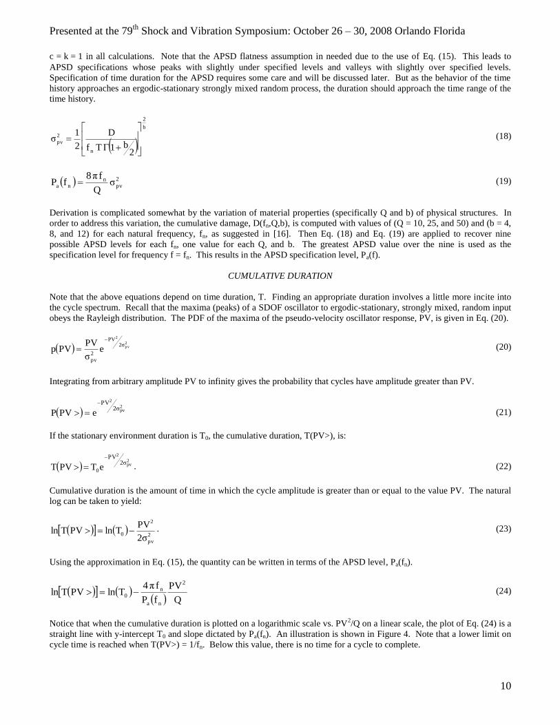
In order to illustrate the benefit of counting rainflow cycles instead of the narrow-band cycles defined in [4], the cycle spectra

is plotted for the oscillator with fn = 1600 Hz, Q = 10. The rainflow spectrum histogram is plotted with bars and the narrow-

band spectrum is plotted with a red line, Figure 3. It can be seen that the damage is under predicted using the narrow-band

cycles approximation suggested in [4]. In fact the cumulative damage, D, using the narrow band cycle count is only 17% of

that using the rainflow cycle count (with b = 8).



9

102

103

10-20

10-15

10-10

10-5

Natural Frequency

Cum

ula

tive D

am

age

Time Domain

Frequency Domain Num.

Frequency Domain C.F.

Figure 2: Fatigue Damage Spectrum

0 1 2 3 4 5 6

x 10-3

0

200

400

600

800

1000

1200

1400

Bin Amplitude

Counts

Rainflow

Narrow Band

Figure 3: Cycle Spectra for fn = 1600 Hz, Q = 10

FATIGUE DAMAGE EQUIVALENT TESTING

INVERTING THE FDS

The concept of the FDS can be used to derive ergodic-stationary, Gaussian random vibration specifications in the form of an

APSD spectrum and associated time duration from non-stationary acceleration environments described by a time history.

Basically, the FDS, D(fn,Q,b), of the time history is computed. Then the APSD level for a damage equivalent Gaussian

random environment can be computed, for each fn, by inverting Eq. (14) and Eq. (15) to yield Eq. (18) and Eq. (19), where



10

c = k = 1 in all calculations. Note that the APSD flatness assumption in needed due to the use of Eq. (15). This leads to

APSD specifications whose peaks with slightly under specified levels and valleys with slightly over specified levels.

Specification of time duration for the APSD requires some care and will be discussed later. But as the behavior of the time

history approaches an ergodic-stationary strongly mixed random process, the duration should approach the time range of the

time history.

b

2

n

2

pv

2b1ΓTf

D

2

1σ

(18)

2

pvn

na σQ

fπ8fP (19)

Derivation is complicated somewhat by the variation of material properties (specifically Q and b) of physical structures. In

order to address this variation, the cumulative damage, D(fn,Q,b), is computed with values of (Q = 10, 25, and 50) and (b = 4,

8, and 12) for each natural frequency, fn, as suggested in [16]. Then Eq. (18) and Eq. (19) are applied to recover nine

possible APSD levels for each fn, one value for each Q, and b. The greatest APSD value over the nine is used as the

specification level for frequency f = fn. This results in the APSD specification level, Pa(f).

CUMULATIVE DURATION

Note that the above equations depend on time duration, T. Finding an appropriate duration involves a little more incite into

the cycle spectrum. Recall that the maxima (peaks) of a SDOF oscillator to ergodic-stationary, strongly mixed, random input

obeys the Rayleigh distribution. The PDF of the maxima of the pseudo-velocity oscillator response, PV, is given in Eq. (20).

2pv

2

2σPV

2

pv

eσ

PVPVp

(20)

Integrating from arbitrary amplitude PV to infinity gives the probability that cycles have amplitude greater than PV.

2pv

2

2σPV

ePVP

(21)

If the stationary environment duration is T0, the cumulative duration, T(PV>), is:

2pv

2

2σPV

eTPVT 0

. (22)

Cumulative duration is the amount of time in which the cycle amplitude is greater than or equal to the value PV. The natural

log can be taken to yield:

2

pv

2

02σ

PVTlnPVTln . (23)

Using the approximation in Eq. (15), the quantity can be written in terms of the APSD level, Pa(fn).

Q

PV

fP

fπ4TlnPVTln

2

na

n0 (24)

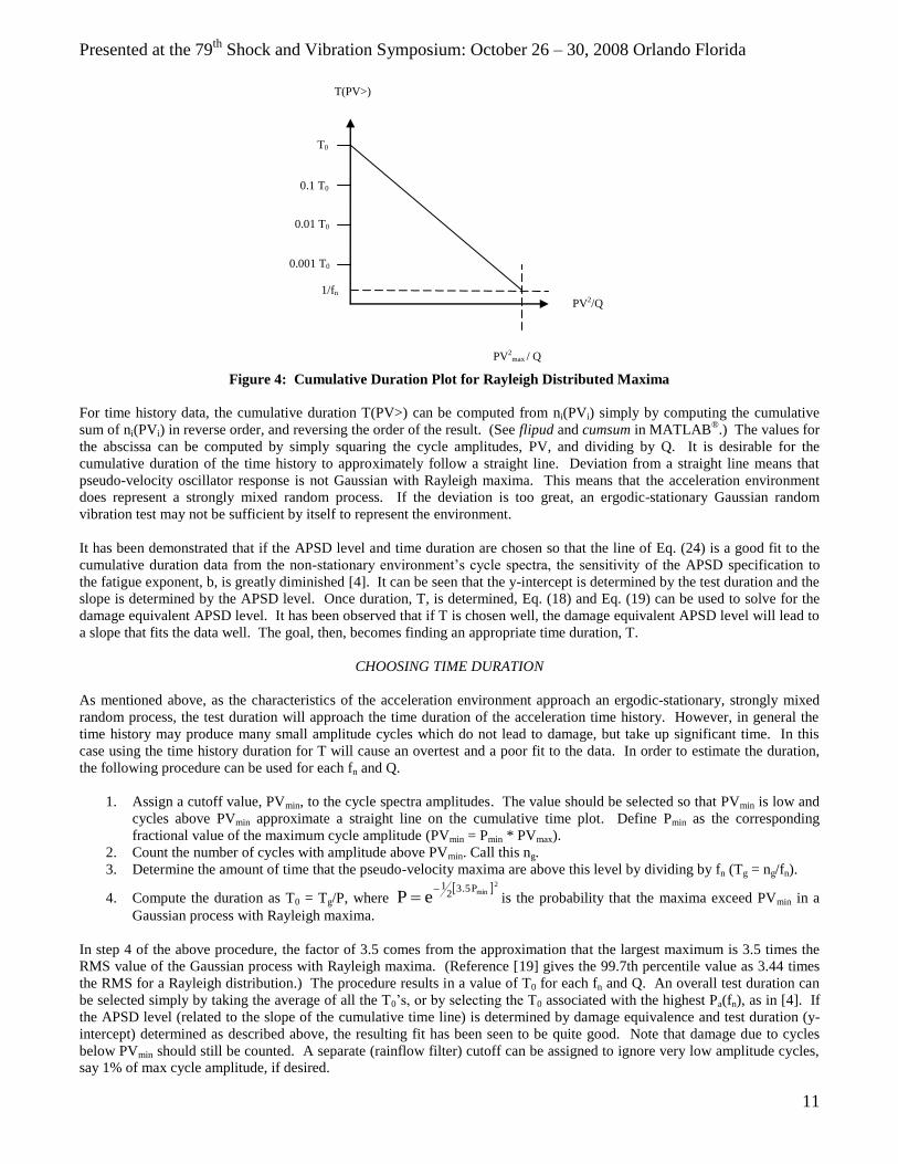
Notice that when the cumulative duration is plotted on a logarithmic scale vs. PV2/Q on a linear scale, the plot of Eq. (24) is a

straight line with y-intercept T0 and slope dictated by Pa(fn). An illustration is shown in Figure 4. Note that a lower limit on

cycle time is reached when T(PV>) = 1/fn. Below this value, there is no time for a cycle to complete.



11

Figure 4: Cumulative Duration Plot for Rayleigh Distributed Maxima

For time history data, the cumulative duration T(PV>) can be computed from ni(PVi) simply by computing the cumulative

sum of ni(PVi) in reverse order, and reversing the order of the result. (See flipud and cumsum in MATLAB®.) The values for

the abscissa can be computed by simply squaring the cycle amplitudes, PV, and dividing by Q. It is desirable for the

cumulative duration of the time history to approximately follow a straight line. Deviation from a straight line means that

pseudo-velocity oscillator response is not Gaussian with Rayleigh maxima. This means that the acceleration environment

does represent a strongly mixed random process. If the deviation is too great, an ergodic-stationary Gaussian random

vibration test may not be sufficient by itself to represent the environment.

It has been demonstrated that if the APSD level and time duration are chosen so that the line of Eq. (24) is a good fit to the

cumulative duration data from the non-stationary environment’s cycle spectra, the sensitivity of the APSD specification to

the fatigue exponent, b, is greatly diminished [4]. It can be seen that the y-intercept is determined by the test duration and the

slope is determined by the APSD level. Once duration, T, is determined, Eq. (18) and Eq. (19) can be used to solve for the

damage equivalent APSD level. It has been observed that if T is chosen well, the damage equivalent APSD level will lead to

a slope that fits the data well. The goal, then, becomes finding an appropriate time duration, T.

CHOOSING TIME DURATION

As mentioned above, as the characteristics of the acceleration environment approach an ergodic-stationary, strongly mixed

random process, the test duration will approach the time duration of the acceleration time history. However, in general the

time history may produce many small amplitude cycles which do not lead to damage, but take up significant time. In this

case using the time history duration for T will cause an overtest and a poor fit to the data. In order to estimate the duration,

the following procedure can be used for each fn and Q.

1. Assign a cutoff value, PVmin, to the cycle spectra amplitudes. The value should be selected so that PVmin is low and

cycles above PVmin approximate a straight line on the cumulative time plot. Define Pmin as the corresponding

fractional value of the maximum cycle amplitude (PVmin = Pmin * PVmax).

2. Count the number of cycles with amplitude above PVmin. Call this ng.

3. Determine the amount of time that the pseudo-velocity maxima are above this level by dividing by fn (Tg = ng/fn).

4. Compute the duration as T0 = Tg/P, where 2

minP3.52

1

eP

is the probability that the maxima exceed PVmin in a

Gaussian process with Rayleigh maxima.

In step 4 of the above procedure, the factor of 3.5 comes from the approximation that the largest maximum is 3.5 times the

RMS value of the Gaussian process with Rayleigh maxima. (Reference [19] gives the 99.7th percentile value as 3.44 times

the RMS for a Rayleigh distribution.) The procedure results in a value of T0 for each fn and Q. An overall test duration can

be selected simply by taking the average of all the T0’s, or by selecting the T0 associated with the highest Pa(fn), as in [4]. If

the APSD level (related to the slope of the cumulative time line) is determined by damage equivalence and test duration (y-

intercept) determined as described above, the resulting fit has been seen to be quite good. Note that damage due to cycles

below PVmin should still be counted. A separate (rainflow filter) cutoff can be assigned to ignore very low amplitude cycles,

say 1% of max cycle amplitude, if desired.

0.001 T0

T(PV>)

PV2/Q

T0

0.1 T0

0.01 T0

1/fn

PV2max / Q



12

By requiring the cumulative duration of the environment data to approximate a straight line and finding T as discussed, the

cycle spectra of the test will approximate that of the environment. In this way some of the temporal characteristics of the

environment are preserved without considering temporal moments.

FDET ALGORITHM

An algorithm was implemented to compute the FDET specification APSD level and duration. The procedure uses two

phases to streamline the process. The algorithm is outlined below.

Phase 1: Compute Cycle Spectra for Each fn and Q

1. Obtain the environment acceleration time history. Detrend and up-sample if needed.

2. Define a range of natural frequencies and logarithmically space fn at 1/12 octaves. Set Q values to [10, 25, 50].

Loop over natural frequencies

Loop over quality factor values

3. Compute pseudo-velocity oscillator response

4. Compute rainflow cycles

5. Rainflow filter if desired, and compute cycle spectrum.

6. Compute T0.

7. Compute overall duration T0ov

(take mean(T0) for example).

8. Check T> vs. PV2/Q plots to see if ergodic-stationary Gaussian random test is sufficient.

Phase 2: Compute Damage for Each fn, Q, and b and Recover Equivalent Pa(fn)

1. Obtain cycle spectra for each fn and Q and T0ov

from phase 1.

2. Define b values as [4, 8, 12].


Loop over quality factor values

Loop over fatigue exponents

3. Compute cumulative damage (equation (10) with c = k = 1)

4. Compute APSD levels, Pa(fn), for each Q and b combination ( equations (18) and (19) with T set to T0ov

.

5. Select the greatest value of Pa(fn) and save the corresponding worst case Q and b as well as corresponding

damage level D(fn,Q,b).

6. Check T> vs. PV2/Q plots with specification line computed from equation (24) drawn in.

7. Refine specification if necessary.

After completion of the algorithm. The FDS can be checked for several fn, Q, b combinations to make sure the FDS of the

test specification envelopes the FDS of the acceleration history.

It can be noted that it is possible to derive a Gaussian APSD environment that is peak-response equivalent to a non-stationary

(or transient) environment described by a base acceleration time history using the SRS and VRS techniques. First the SRS

can be computed from the time history. Then, if the assumption on flatness of the APSD holds, Eq. (2) can be inverted and

used to solve for the APSD level at each natural frequency. Therefore, the above procedure can be (slightly) modified for

obtaining a peak-response equivalent environment.

REFINING THE FDET SPECIFICATION

In Phase 2 of the procedure, the APSD specification is computed from the FDS using the approximation in equation (19),

which is valid under the flatness assumption. The flatness assumption does not hold when the spectral content of the

environment varies significantly in the vicinity of the half-power bandwidths of the oscillators. In such cases, the computed

APSD specification will be prone to error. Step 7 of Phase 2 states that the specification should be refined if error is

significant. A method for refining the APSD is discussed in the remainder of this section.

Error in the APSD specification, Pa(fn), computed in Step 4 of Phase 2 can be evaluated by, first, computing the FDS of the

APSD specification, Dspec(fn,Q,b), via Eq. (14) and Eq. (16). Here, Q and b are the worst case values stored in Step 5 of

Phase 2. The FDS will not generally be the same as the FDS computed from the time history and stored in Step 5 in Phase 2,

D(fn,Q,b), due to the fact that the spectral shape is accounted for in Eq. (16). The error, D(fn,Q,b) - Dspec(fn,Q,b), can be

evaluated by taking the 2-norm, for example.



13

If error levels are not acceptable, the APSD specification can be refined until error levels are within a defined tolerance using

a Newton-Raphson method at each frequency. The method is outlined below:

1. Compute the FDS of the APSD specification, Dspec(fn,Q,b), via Eq. (14) and Eq. (16), with worst case Q and b.


2. Compute damage error, error(fn,Q,b) = D(fn,Q,b) - Dspec(fn,Q,b).

3. Compute slope, slope(fn) = ΔD(fn,Q,b)/ Δ Pa(fn) numerically, in the vicinity of fn.

3b. Alternatively, slope may be approximated in closed form by combining Eq. (14) and Eq. (15) and differentiating,

.fP2

b1Γ

f4π

Qk

2c

bTffslope

12

b

n

2b

n

bnn

Here, worst case Q and b are used.

4. Update the APSD specification, Pa(fn) = Pa(fn) + error(fn,Q,b)/slope(fn).

5. Compute FDS of the new APSD specification, Dspec(fn,Q,b), via Eq. (14) and Eq. (16), with worst case Q and b.

6. Compute damage error, error(fn,Q,b) = D(fn,Q,b) - Dspec(fn,Q,b).

7. Evaluate the error magnitude by taking the 2-norm of error(fn,Q,b).

8. If error magnitude is greater than a specified tolerance, go to step 3.

In this way the APSD specification, Pa(fn), computed in Step 4 of Phase 2 acts as an initial guess for the Newton method. It

is important to note that the closed form approximation for slope is not as accurate when the flatness assumption is violated.

It was observed during simulations that the inaccuracy leads to instabilities. To remove the instabilities, it was necessary to

multiply the update (last term in the equation in step 4.) by a relaxation parameter, μ. Values for the parameter may range

from 0.1 ≤ μ ≤ 0.5. It was verified that when the slope is evaluated numerically, no relaxation is necessary. It is also

important to provide a mechanism for preventing Pa(fn) from becoming negative. To accomplish this, negative values can be

found and replaced with small positive values after Step 4.

FATIGUE DAMAGE EQUIVALENT TESTING EXAMPLES

In this section some examples of the FDET method are given. In some cases, APSD levels are compared with APSD levels

derived with a traditional maximax approach [19]. The maximax APSD was derived by dividing the acceleration history into

time ranges with 50% overlap, computing the APSD, averaging in 1/6 octave bands, and taking the envelope of the 1/6th

octave averaged spectra.

GAUSSIAN RANDOM ACCELERATION HISTORY WITH PRESCRIBED APSD

The acceleration time history environment with associated APSD, shown in Figure 1, was used as a test case to verify the

algorithm’s concepts and code. It was expected that the resulting test specification and duration would be given by the APSD

values in Table 1 with duration equal to the time history duration length, 20.007 seconds.

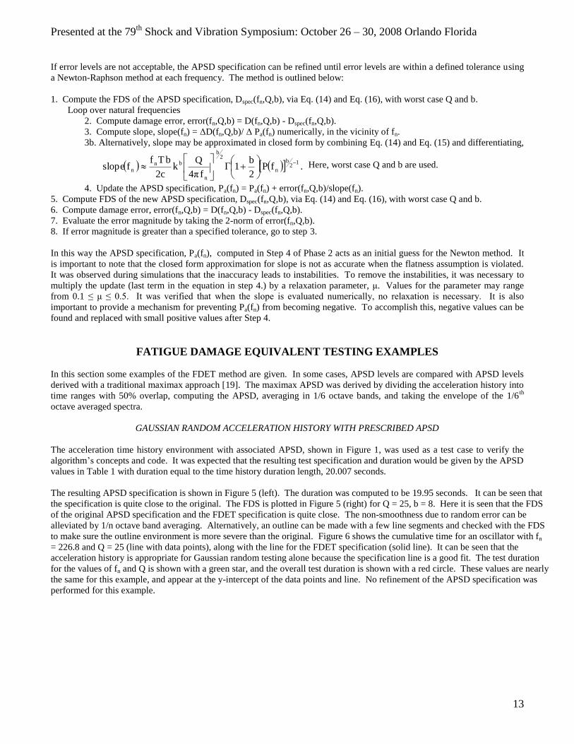
The resulting APSD specification is shown in Figure 5 (left). The duration was computed to be 19.95 seconds. It can be seen that

the specification is quite close to the original. The FDS is plotted in Figure 5 (right) for Q = 25, b = 8. Here it is seen that the FDS

of the original APSD specification and the FDET specification is quite close. The non-smoothness due to random error can be

alleviated by 1/n octave band averaging. Alternatively, an outline can be made with a few line segments and checked with the FDS

to make sure the outline environment is more severe than the original. Figure 6 shows the cumulative time for an oscillator with fn

= 226.8 and Q = 25 (line with data points), along with the line for the FDET specification (solid line). It can be seen that the

acceleration history is appropriate for Gaussian random testing alone because the specification line is a good fit. The test duration

for the values of fn and Q is shown with a green star, and the overall test duration is shown with a red circle. These values are nearly

the same for this example, and appear at the y-intercept of the data points and line. No refinement of the APSD specification was

performed for this example.



14

102

103

10-2

10-1

Frequency [Hz]

AP

SD

[G

2 /

Hz]

Acceleration PSD

FDET Spec

Original

102

103

10-20

10-15

10-10

10-5

Frequency [Hz]

Cum

ula

tive D

am

age

Fatigue Damage Spectrum

FDET Spec

Original

Figure 5: FDET Specification (Left) and FDS (Right)

0 1 2

x 10-4

10-2

10-1

100

101

PV2/Q

T(P

V>

)

fnp = 226.274 , qfp = 25.000

Sim. Counts

Spec. Counts

T0

T

Figure 6: Cumulative Time Plot

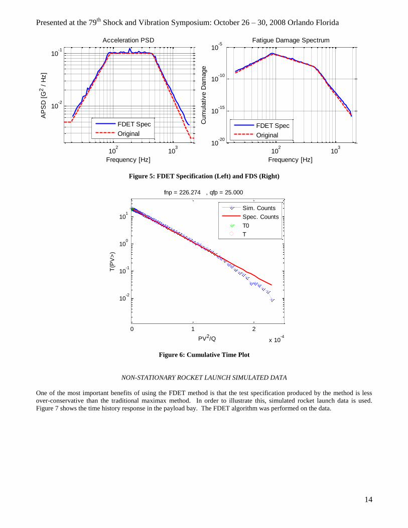
NON-STATIONARY ROCKET LAUNCH SIMULATED DATA

One of the most important benefits of using the FDET method is that the test specification produced by the method is less

over-conservative than the traditional maximax method. In order to illustrate this, simulated rocket launch data is used.

Figure 7 shows the time history response in the payload bay. The FDET algorithm was performed on the data.



15

0 10 20 30 40 50 60 70 80 90 100-40

-20

0

20

40

Time [Sec]

Am

plit

ude [

G's

]

Time History

Figure 7: Simulated Rocket Launch Time History

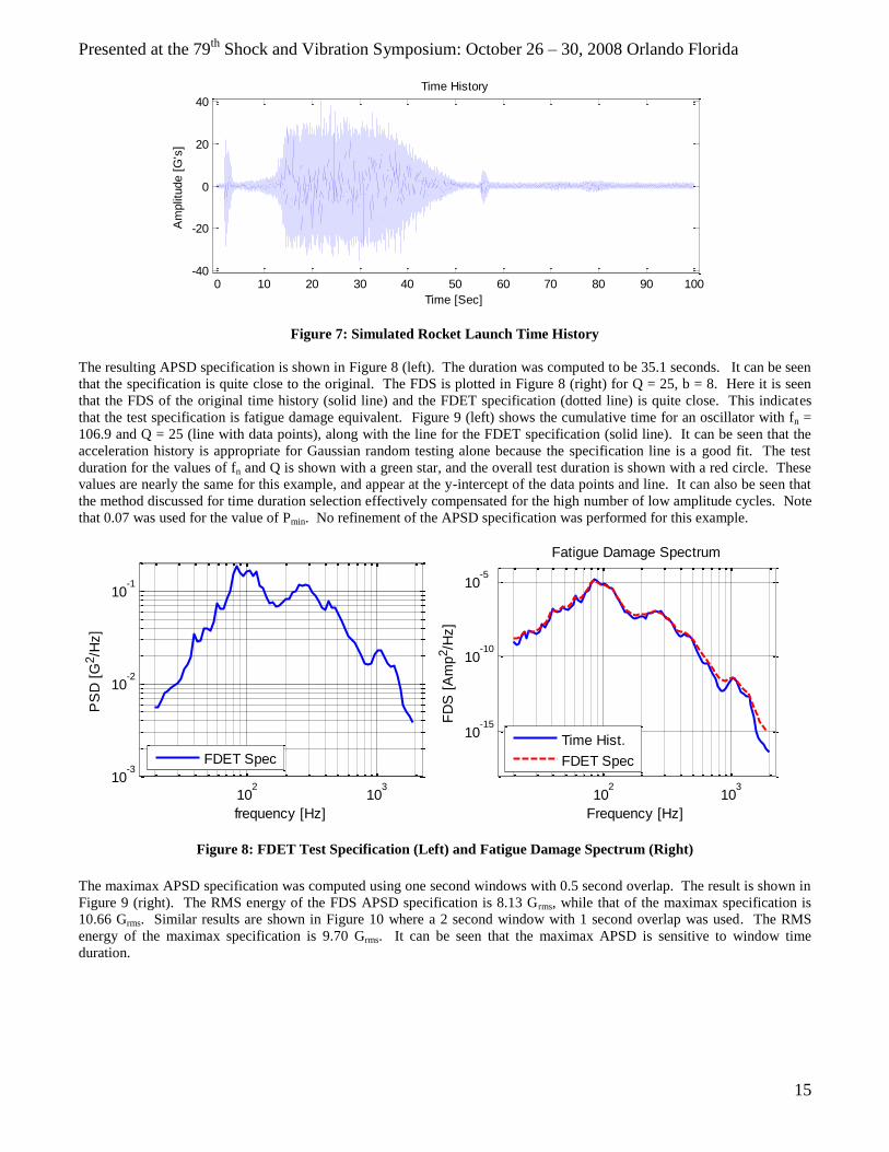
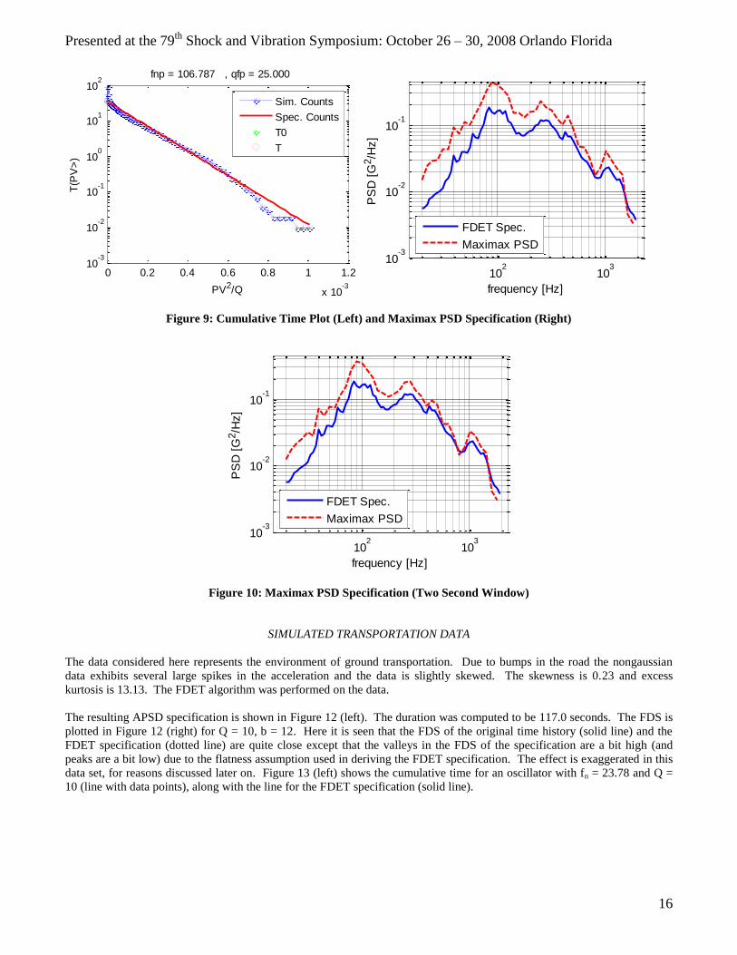
The resulting APSD specification is shown in Figure 8 (left). The duration was computed to be 35.1 seconds. It can be seen

that the specification is quite close to the original. The FDS is plotted in Figure 8 (right) for Q = 25, b = 8. Here it is seen

that the FDS of the original time history (solid line) and the FDET specification (dotted line) is quite close. This indicates

that the test specification is fatigue damage equivalent. Figure 9 (left) shows the cumulative time for an oscillator with fn =

106.9 and Q = 25 (line with data points), along with the line for the FDET specification (solid line). It can be seen that the

acceleration history is appropriate for Gaussian random testing alone because the specification line is a good fit. The test

duration for the values of fn and Q is shown with a green star, and the overall test duration is shown with a red circle. These

values are nearly the same for this example, and appear at the y-intercept of the data points and line. It can also be seen that

the method discussed for time duration selection effectively compensated for the high number of low amplitude cycles. Note

that 0.07 was used for the value of Pmin. No refinement of the APSD specification was performed for this example.

102

103

10-3

10-2

10-1

frequency [Hz]

PS

D [

G2/H

z]

FDET Spec

102

103

10-15

10-10

10-5

Frequency [Hz]

FD

S [

Am

p2/H

z]


Time Hist.

FDET Spec

Figure 8: FDET Test Specification (Left) and Fatigue Damage Spectrum (Right)

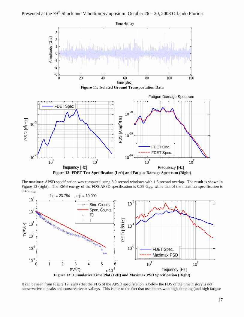
The maximax APSD specification was computed using one second windows with 0.5 second overlap. The result is shown in

Figure 9 (right). The RMS energy of the FDS APSD specification is 8.13 Grms, while that of the maximax specification is

10.66 Grms. Similar results are shown in Figure 10 where a 2 second window with 1 second overlap was used. The RMS

energy of the maximax specification is 9.70 Grms. It can be seen that the maximax APSD is sensitive to window time

duration.



16

0 0.2 0.4 0.6 0.8 1 1.2

x 10-3

10-3

10-2

10-1

100

101

102

PV2/Q

T(P

V>

)fnp = 106.787 , qfp = 25.000

Sim. Counts

Spec. Counts

T0

T

102

103

10-3

10-2

10-1

frequency [Hz]

PS

D [

G2/H

z]

FDET Spec.

Maximax PSD

Figure 9: Cumulative Time Plot (Left) and Maximax PSD Specification (Right)

102

103

10-3

10-2

10-1

frequency [Hz]

PS

D [

G2/H

z]

FDET Spec.

Maximax PSD

Figure 10: Maximax PSD Specification (Two Second Window)

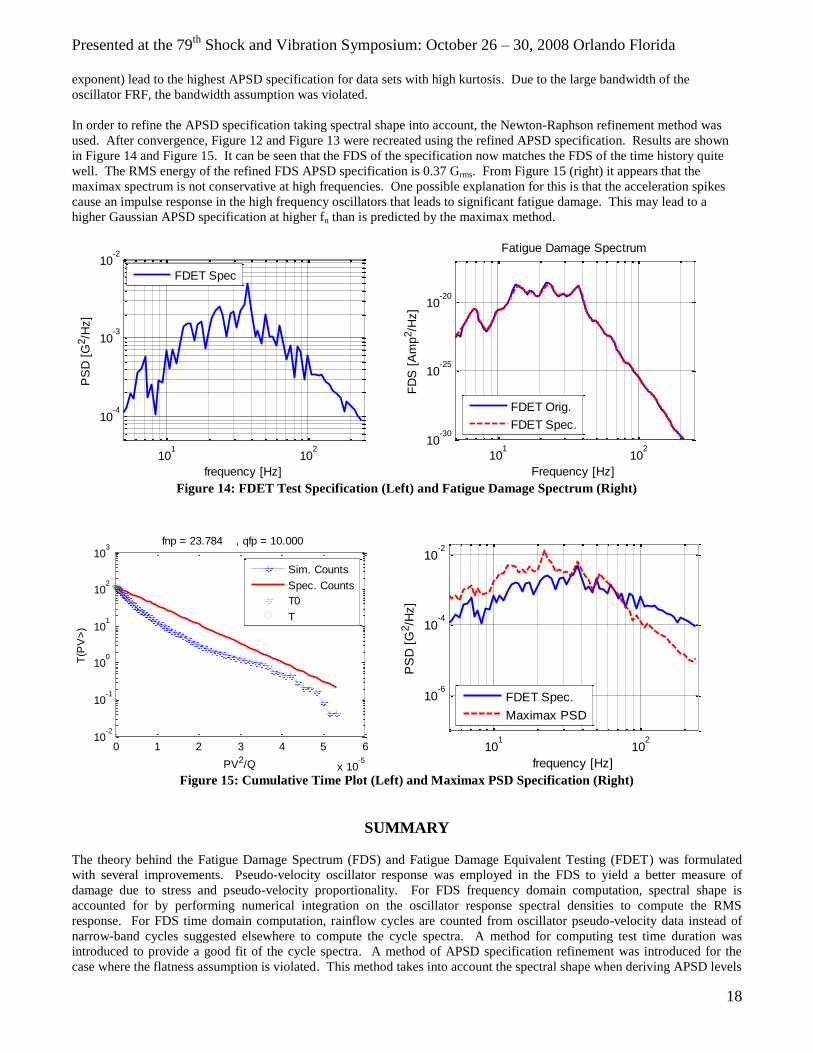
SIMULATED TRANSPORTATION DATA

The data considered here represents the environment of ground transportation. Due to bumps in the road the nongaussian

data exhibits several large spikes in the acceleration and the data is slightly skewed. The skewness is 0.23 and excess

kurtosis is 13.13. The FDET algorithm was performed on the data.

The resulting APSD specification is shown in Figure 12 (left). The duration was computed to be 117.0 seconds. The FDS is

plotted in Figure 12 (right) for Q = 10, b = 12. Here it is seen that the FDS of the original time history (solid line) and the

FDET specification (dotted line) are quite close except that the valleys in the FDS of the specification are a bit high (and

peaks are a bit low) due to the flatness assumption used in deriving the FDET specification. The effect is exaggerated in this

data set, for reasons discussed later on. Figure 13 (left) shows the cumulative time for an oscillator with fn = 23.78 and Q =

10 (line with data points), along with the line for the FDET specification (solid line).



17

0 20 40 60 80 100 120-3

-2

-1

0

1

2

3

Time [Sec]

Am

plitu

de [

G's

]

Time History

Figure 11: Isolated Ground Transportation Data

101

102

10-4

10-3

frequency [Hz]

PS

D [

G2/H

z]

FDET Spec

101

102

10-30

10-25

10-20

Frequency [Hz]

FD

S [

Am

p2/H

z]


FDET Orig.

FDET Spec.


The maximax APSD specification was computed using 3.0 second windows with 1.5 second overlap. The result is shown in

Figure 13 (right). The RMS energy of the FDS APSD specification is 0.38 Grms, while that of the maximax specification is

0.45 Grms.

0 1 2 3 4 5 6

x 10-5

10-2

10-1

100

101

102

103

PV2/Q

T(P

V>

)

fnp = 23.784 , qfp = 10.000

Sim. Counts

Spec. Counts

T0

T

101

102

10-6

10-4

10-2

frequency [Hz]

PS

D [

G2/H

z]

FDET Spec.

Maximax PSD


It can be seen from Figure 12 (right) that the FDS of the APSD specification is below the FDS of the time history is not

conservative at peaks and conservative at valleys. This is due to the fact that oscillators with high damping (and high fatigue



18

exponent) lead to the highest APSD specification for data sets with high kurtosis. Due to the large bandwidth of the

oscillator FRF, the bandwidth assumption was violated.

In order to refine the APSD specification taking spectral shape into account, the Newton-Raphson refinement method was

used. After convergence, Figure 12 and Figure 13 were recreated using the refined APSD specification. Results are shown

in Figure 14 and Figure 15. It can be seen that the FDS of the specification now matches the FDS of the time history quite

well. The RMS energy of the refined FDS APSD specification is 0.37 Grms. From Figure 15 (right) it appears that the

maximax spectrum is not conservative at high frequencies. One possible explanation for this is that the acceleration spikes

cause an impulse response in the high frequency oscillators that leads to significant fatigue damage. This may lead to a

higher Gaussian APSD specification at higher fn than is predicted by the maximax method.

101

102

10-4

10-3

10-2

frequency [Hz]

PS

D [

G2/H

z]

FDET Spec

101

102

10-30

10-25

10-20

Frequency [Hz]

FD

S [

Am

p2/H

z]


FDET Orig.

FDET Spec.


0 1 2 3 4 5 6

x 10-5

10-2

10-1

100

101

102

103

PV2/Q

T(P

V>

)

fnp = 23.784 , qfp = 10.000

Sim. Counts

Spec. Counts

T0

T

101

102

10-6

10-4

10-2

frequency [Hz]

PS

D [

G2/H

z]

FDET Spec.

Maximax PSD


SUMMARY

The theory behind the Fatigue Damage Spectrum (FDS) and Fatigue Damage Equivalent Testing (FDET) was formulated

with several improvements. Pseudo-velocity oscillator response was employed in the FDS to yield a better measure of

damage due to stress and pseudo-velocity proportionality. For FDS frequency domain computation, spectral shape is

accounted for by performing numerical integration on the oscillator response spectral densities to compute the RMS

response. For FDS time domain computation, rainflow cycles are counted from oscillator pseudo-velocity data instead of

narrow-band cycles suggested elsewhere to compute the cycle spectra. A method for computing test time duration was

introduced to provide a good fit of the cycle spectra. A method of APSD specification refinement was introduced for the

case where the flatness assumption is violated. This method takes into account the spectral shape when deriving APSD levels



19

from the FDS. Examples were given to demonstrate the equivalence of computing the FDS in the time domain and

frequency domain and illustrate the advantages of FDET over traditional maximax APSD specification. Computational

techniques were discussed for efficient calculation in MATLAB®.

REFERENCES

[1] G. R. Henderson and A. G. Piersol, “Fatigue Damage Related Descriptor for Random Vibration Test Environments,”

Sound and Vibration, October, 1995, pp. 20-24.

[2] G. R. Henderson, “Fatigue Damage Descriptors for HALT and HASS Testing,” Sound and Vibration, August, 2004.

[3] K. Ahlin, “Comparison of Test Specifications and Measured Field Data,” Sound and Vibration, September, 2006, pp.

22-25.

[4] J. F. Miskel III, “Fatigue-Based Random Vibration and Acoustic Test Specification,” Master’s Thesis, Department of

Mechanical Engineering, Massachusetts Institute of Technology, May, 1994.

[5] S. Rubin, “Damage-Based Analysis Tool for Flight Vibroacoustic Data,” Proceedings of the 19th

Aerospace Testing

Seminar, Manhattan Beach, CA, October 2-5, 2000.

[6] A. Halfpenny, “Accelerated Vibration Testing Based on Fatigue Damage Spectra,” Aerospace Testing Expo,

Hamburg, Germany, April 4-6, 2006.

[7] S. H. Crandall, “Relationship between Stress and Velocity in Resonant Vibration,” Journal of Acoustical Society of

America, 1962, Vol. 34(12), pp. 31-49.

[8] D. O. Smallwood, “An Improved Recursive Formula for Calculating Shock Response Spectra,” 51st Shock and

Vibration Bulletin, 1981, Vol 51(2), pp. 211-217.

[9] T. Irvine, “An Introduction to the Vibration Response Spectrum Rev C,” Vibrationdata Tutorials,

http://www.vibrationdata.com/tutorials2/vrs.pdf, June 14, 2000.

[10] D. O. Smallwood, “Characterization and Simulation of Transient Vibrations Using Band Limited Moments,” Shock

and Vibration, 1994, Vol. 1(6), pp. 507-527.

[11] H. A. Gaberson and R. H. Chalmers, “Modal Velocity as a Criterion of Shock Severity,” Shock and Vibration Bulletin,

1969, Vol. 40(2), pp. 31-49.

[12] H. A. Gaberson and R. H. Chalmers, “Reasons for Presenting Shock Spectra with Velocity as the Ordinate,”

Proceedings of the 66th

Shock and Vibration Symposium, Biloxi, Mississippi, Oct. 30 – Nov. 3, 1995, pp. 181-191.

[13] F. V. Hunt, “Stress and Strain Limits on the Attainable Velocity in Mechanical Vibration,” Journal of the Acoustical

Society of America, 1966, Vol. 32(9), pp. 1123-1128.

[14] K. Ahlin, “Shock Response Spectrum Calculation – An Improvement of the Smallwood Algorithm,” 70th

Shock &

Vibration Symposium, Albuquerque, NM, November 15-19, 1999.

[15] D. Benasciutti, “Fatigue Analysis of Random Loadings,” Ph. D. Thesis, Department of Engineering Graduate School

in Civil and Industrial Engineering, University of Ferrara, Italy, December, 2004.

[16] S. J. DiMaggio, B. H. Sako and S. Rubin, “Analysis of Nonstationary Vibroacoustic Flight Data Using a Damage

Potential Basis,” Proceedings of the 44th

AIAA/ASME/ASCE/AHS/ASC Structures, Structural Dynamics, and Materials

Conference, Norfolk, Virginia, April 7-10, 2003.

[17] A. Halfpenny, “A Frequency Domain Approach for Fatigue Life Estimation From Finite Element Analysis,”

International Conference of Damage Assessment of Structures, Dublin, Ireland, June, 1999.



20

[18] S. H. Crandall, and W. D. Mark, 1963, Random Vibrations in Mechanical Systems, Academic Press, New York.

[19] H. Himelblau, D. L. Dern, J. E. Manning, A. G. Piersol, and S. Rubin, “Dynamic Environmental Criteria,” National

Aeronautics and Space Administration NASA-HDBK-7005, March, 2001.

[20] C. Amzallag, J. P. Gerey, J. L. Robert, and J. Bahauaud, “Standardization of the Rainflow Counting Method for

Fatigue Analysis,” International Journal of Fatigue, 1994, Vol. 16(4), pp. 287-293.

[21] J. S. Bendat and A. G. Piersol, 2000, Random Data Analysis and Measurement Proceedures, (3rd

ed.), John Wiley &

Sons, Inc., New York.

[22] T. Irvine, “An Introduction to the Shock Response Spectrum Rev P,” Vibrationdata Tutorials,

http://www.vibrationdata.com/tutorials2/srs_intr.pdf, May 24, 2002.

[23] A. Papoulis, “Narrow-Band Systems and Gaussianity,” Rome Air Development Center RADC-TR-71-225, Griffiss

AFB, New York, 1971.

[24] D. S. Steinberg, 2000, Vibration Analysis for Electronic Equipment, (3rd

ed.), John Wiley & Sons, Inc., New York.

The Fatigue Damage Spectrum and Fatigue Damage Equivalent ... · Presented at the 79th Shock and...

Documents

Transcript of The Fatigue Damage Spectrum and Fatigue Damage Equivalent ... · Presented at the 79th Shock and...