The Factors Influencing Satisfaction with Public City ... · The Factors Influencing Satisfaction...

Journal of Competitiveness 1�

The Factors Influencing Satisfaction with Public City Transport: A Structural Equation Modelling Approach

Pawlasová Pavlína

AbstractSatisfaction is one of the key factors which influences customer loyalty. We assume that the satis-fied customer will be willing to use the ssame service provider again. The overall passengers´ satisfaction with public city transport may be affected by the overall service quality. Frequency, punctuality, cleanliness in the vehicle, proximity, speed, fare, accessibility and safety of trans-port, information and other factors can influence passengers´ satisfaction. The aim of this paper is to quantify factors and identify the most important factors influencing customer satisfaction with public city transport within conditions of the Czech Republic. Two methods of analysis are applied in order to fulfil the aim. The method of factor analysis and the method Varimax were used in order to categorize variables according to their mutual relations. The method of structural equation modelling was used to evaluate the factors and validate the model. Then, the optimal model was found. The logistic parameters, including service continuity and frequency, and service, including information rate, station proximity and vehicle cleanliness, are the factors influencing passengers´ satisfaction on a large scale.

Keywords: factor analysis, public transport, satisfaction, structural equation modelling JEL Classification: M31, M37

1. INTRODUCTIONThe public city transport is very important for all cities, mainly for all big cities and tourist cen-tres. When inhabitants use public transport vehicles instead of the private cars the environment pollution is reduced and also the noise in the city is lower. Also tourists can appreciate cities and tourist centres with simple and customer friendly public transport. Therefore it is important to improve the public transport services.

If we agree with Zamazalová (2009) that a high consumer satisfaction rate contributes signifi-cantly to consumer loyalty to the service provider, service providers should try to achieve the maximum user satisfaction with services, products or purchases. According to Shiau & Luo (2012) consumer satisfaction helps companies to establish long-term relationships with consum-ers. Also the success of a public transport system depends on the number of passengers which the system is able to attract and retain. Therefore the quality of a offered services becomes the issue of maximum importance (de Oña, de Oña, Eboli & Mazzulla, 2013).

The aim of this paper is to quantify factors and identify the most important factors influencing customer satisfaction with public city transport services in the Czech Republic. The method of factor analysis with method Varimax and the method of structural equation modelling were ap-plied to evaluate the factors and validate the proposed model.

▪

Journal of Competitiveness Vol. 7, Issue 4, pp. 18 - 32, December 2015 ISSN 1804-171X (Print), ISSN 1804-1728 (On-line), DOI: 10.7441/joc.2015.04.02

joc4-2015_v2b.indd 18 31.12.2015 13:03:50

1�

The result of this research can help the public transport providers to improve their services. It is important to attract many passengers mainly because of decrease in the number of cars in the cities, reduction of the environment pollution and also because of the noise abatement. Accord-ing to a recent study by Replogle and Fultorn (2014) the urban passenger transport emissions can be reduced by 40 percents by 2050 if the use of public city transport, walking and cycling in cities expands.

2. THEORETICAL BACKGROUND OF THE USERS´ SATISFACTION MEASUREMENTMarketing research measures customer satisfaction after a purchase, in this case after a service execution. Satisfaction can be described as the difference between consumer/passenger expec-tation and actual satisfaction (Shiau & Luo, 2012). Satisfaction with public transport services can be influenced by the service quality that consists of many factors (de Oña, de Oña, Eboli & Mazzulla, 2013).

Public city transport in most Western countries has a specific aspect. Public transport in these countries is provided by operators’ action under a contract with a public transport authority and these services are offered by private or semi-public contractors operating in almost monopolistic conditions. It means that there is not competitive market with requirements in meeting passen-gers’ needs. That is why operators can incline to focus on the needs of the public transport au-thority instead of the needs of the passengers. Therefore the view of the customer is often omit-ted whereas in economics and marketing this kind of view is widely studied (Mouwen, 2015).

If the service quality is measured from the customers´ perspective, the most important is the passengers´ perceptions about the each factor characterizing the service. However it is not only important to know the perceptions about the factors of quality, but the most important is to identify which factors have the highest influence on the global assessment of the service and which factors have the lowest influence on it. Nowadays asking customers to express their opin-ions about the importance of each service attribute is frequently used, but it can lead to the er-roneous estimation, because some factors can be rated as important even though they have little influence on the overall satisfaction, or they are important only in one of the moments of the assessment (before or after thinking) (de Oña, de Oña, & Calvo, 2012; de Oña, de Oña, Eboli & Mazzulla, 2013). Therefore it is recommended to use one of the derived methods, which de-termine the importance of the factors by statistically testing the strength of the relation of the individual factors with the overall satisfaction (Weinstein, 2000).

In de Oña, de Oña, Eboli and Mazzulla (2013) and also in Antonucci, L. et al. (2014) there was the method of structural equation modelling applied in order to measure passengers’ satisfaction with public city transport services and in order to verify how much some service characteristics could influence the perceived quality. All these authors claim that factors affecting customer satisfaction with public city transport can be grouped into latent variables consisting service organisation, safety and reliability, human resources and comfort and cleanliness.

joc4-2015_v2b.indd 19 31.12.2015 13:03:50

Journal of Competitiveness �0

De Oña, de Oña, Eboli and Mazzulla (2013) found that the variable Service, including speed, frequency, punctuality of transport and information, is the factor which influences users’ sat-isfaction in the highest rate. Other variables Comfort and Personnel are not so important. It is important to note that these results are useful only for Spanish public transport services because the respondents of this research were only passengers of the bus transit services in Spain (de Oña, de Oña, Eboli & Mazzulla, 2013).

Antonucci, L. et al. (2014) applied in their study an explorative factorial analysis and a structural equation model and they found that the Italian passengers are very sensitive to the level of the service organization and to the way the service is delivered. It means the punctuality and regular-ity and short waiting time are very important factors determining the customer satisfaction. But the public transport authority should not omit also the safety and reliability of buses, the level of comfort and cleanliness and the professionalism and courtesy of staff, because these factors had also a big weight to determine the customer satisfaction.

Also Mouwen (2015) focused on customer view on public city transport and also on drivers of customer satisfaction with public transport services in the Netherlands. It was found that overall satisfaction with public city transport is influenced the most by service attributes such as on-time performance, travel speed and service frequency, followed by personnel attributed (driver behaviour) and vehicle cleanliness. It is important to note that these results are useful mainly for Dutch public transport services because the Netherland is specific with the high rate of cycling popularity and high public transport fare.

In this paper, there was designed the model according to the structure of the model designed by de Oña, de Oña, Eboli and Mazzulla (2013) at first and this original model was tested in the con-ditions of the Czech Republic. It means that the observed variables were creating latent variables Service, Comfort and Personnel. It was found the model with these designed latent variables is not optimal for describing of the behaviour of the Czech passengers. There can be some differ-ences between Czech and Spanish public transport system and customers that can cause that the model designed by de Oña, de Oña, Eboli and Mazzulla (2013) is not optimal for Czech passen-gers. It is possible to mention different climate, different buying behaviour, different travelling habits or different structure of passengers, mainly because of high number of tourists. That is why the methods of factor analysis and structural equation modelling were used in this paper. According to de Oña, de Oña, Eboli and Mazzulla (2013) and also Antonucci, L. et al. (2014) the method of structural equation modelling is appropriate for describing a complex phenomenon like transit passenger perception of the used service.

3. DATA COLLECTION AND RESEARCH METHODThe purpose of this research was the identification of the importance of the factors influenc-ing Czech passengers’ satisfaction with public transport services. A factor analysis with method Varimax was used in order to categorize variables according to their mutual relations. A struc-tural equation modelling (SEM) was used in order to evaluate the proposed model and find the optimal model with the most significant factors.

joc4-2015_v2b.indd 20 31.12.2015 13:03:50

�1

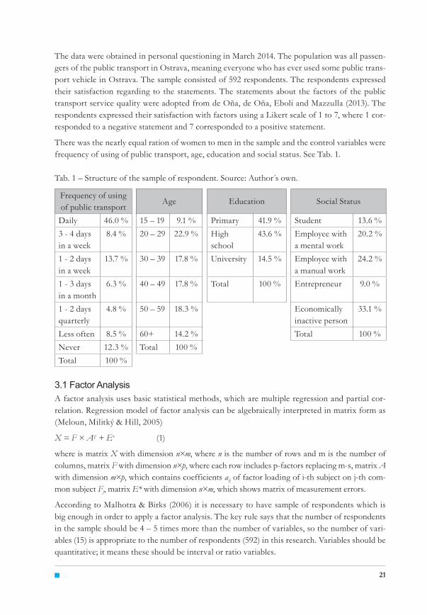
The data were obtained in personal questioning in March 2014. The population was all passen-gers of the public transport in Ostrava, meaning everyone who has ever used some public trans-port vehicle in Ostrava. The sample consisted of 592 respondents. The respondents expressed their satisfaction regarding to the statements. The statements about the factors of the public transport service quality were adopted from de Oña, de Oña, Eboli and Mazzulla (2013). The respondents expressed their satisfaction with factors using a Likert scale of 1 to 7, where 1 cor-responded to a negative statement and 7 corresponded to a positive statement.

There was the nearly equal ration of women to men in the sample and the control variables were frequency of using of public transport, age, education and social status. See Tab. 1.

Tab. 1 – Structure of the sample of respondent. Source: Author s own.

Frequency of using of public transport

Age Education Social Status

Daily 46.0 % 15 – 19 9.1 % Primary 41.9 % Student 13.6 %3 - 4 days in a week

8.4 % 20 – 29 22.9 % High school

43.6 % Employee with a mental work

20.2 %

1 - 2 days in a week

13.7 % 30 – 39 17.8 % University 14.5 % Employee with a manual work

24.2 %

1 - 3 days in a month

6.3 % 40 – 49 17.8 % Total 100 % Entrepreneur 9.0 %

1 - 2 days quarterly

4.8 % 50 – 59 18.3 % Economically inactive person

33.1 %

Less often 8.5 % 60+ 14.2 % Total 100 %Never 12.3 % Total 100 %Total 100 %

3.1 Factor AnalysisA factor analysis uses basic statistical methods, which are multiple regression and partial cor-relation. Regression model of factor analysis can be algebraically interpreted in matrix form as (Meloun, Militký & Hill, 2005)

X = F × AT + E* (1)

where is matrix X with dimension n×m, where n is the number of rows and m is the number of columns, matrix F with dimension n×p, where each row includes p-factors replacing m-s, matrix A with dimension m×p, which contains coefficients aij of factor loading of i-th subject on j-th com-mon subject Fj, matrix E* with dimension n×m, which shows matrix of measurement errors.

According to Malhotra & Birks (2006) it is necessary to have sample of respondents which is big enough in order to apply a factor analysis. The key rule says that the number of respondents in the sample should be 4 – 5 times more than the number of variables, so the number of vari-ables (15) is appropriate to the number of respondents (592) in this research. Variables should be quantitative; it means these should be interval or ratio variables.

joc4-2015_v2b.indd 21 31.12.2015 13:03:51

Journal of Competitiveness ��

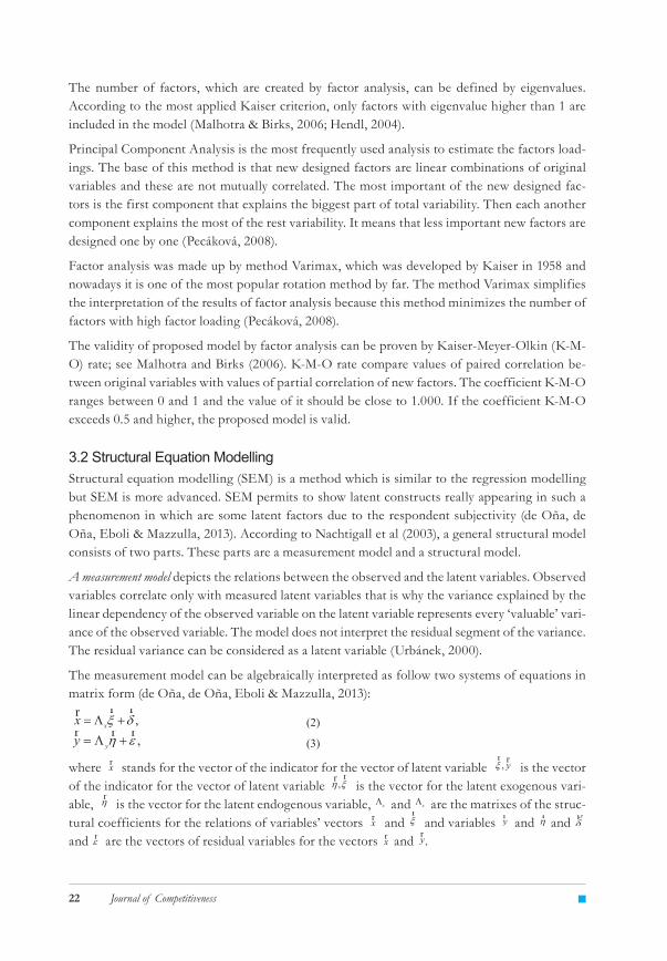
The number of factors, which are created by factor analysis, can be defined by eigenvalues. According to the most applied Kaiser criterion, only factors with eigenvalue higher than 1 are included in the model (Malhotra & Birks, 2006; Hendl, 2004).

Principal Component Analysis is the most frequently used analysis to estimate the factors load-ings. The base of this method is that new designed factors are linear combinations of original variables and these are not mutually correlated. The most important of the new designed fac-tors is the first component that explains the biggest part of total variability. Then each another component explains the most of the rest variability. It means that less important new factors are designed one by one (Pecáková, 2008).

Factor analysis was made up by method Varimax, which was developed by Kaiser in 1958 and nowadays it is one of the most popular rotation method by far. The method Varimax simplifies the interpretation of the results of factor analysis because this method minimizes the number of factors with high factor loading (Pecáková, 2008).

The validity of proposed model by factor analysis can be proven by Kaiser-Meyer-Olkin (K-M-O) rate; see Malhotra and Birks (2006). K-M-O rate compare values of paired correlation be-tween original variables with values of partial correlation of new factors. The coefficient K-M-O ranges between 0 and 1 and the value of it should be close to 1.000. If the coefficient K-M-O exceeds 0.5 and higher, the proposed model is valid.

3.2 Structural Equation ModellingStructural equation modelling (SEM) is a method which is similar to the regression modelling but SEM is more advanced. SEM permits to show latent constructs really appearing in such a phenomenon in which are some latent factors due to the respondent subjectivity (de Oña, de Oña, Eboli & Mazzulla, 2013). According to Nachtigall et al (2003), a general structural model consists of two parts. These parts are a measurement model and a structural model.

A measurement model depicts the relations between the observed and the latent variables. Observed variables correlate only with measured latent variables that is why the variance explained by the linear dependency of the observed variable on the latent variable represents every ‘valuable’ vari-ance of the observed variable. The model does not interpret the residual segment of the variance. The residual variance can be considered as a latent variable (Urbánek, 2000).

The measurement model can be algebraically interpreted as follow two systems of equations in matrix form (de Oña, de Oña, Eboli & Mazzulla, 2013):

,xxr rr

(2),yy r rr

(3)

where xr stands for the vector of the indicator for the vector of latent variable , yr r

is the

vector of the indicator for the vector of latent variable ,rr

is the vector for the latent

exogenous variable, r

is the vector for the latent endogenous variable, x and y are the

matrixes of the structural coefficients for the relations of variables’ vectors xr and r and

variables yr and ,rand and

r xr and .yr

and

stands for the vector of the indicator for the vector of latent variable xr stands for the vector of the indicator for the vector of latent variable , yr r

is the







r xr and .yr

and

is the vector of the indicator for the vector of latent variable

xr stands for the vector of the indicator for the vector of latent variable , yr r

is the







r xr and .yr

and

is the vector for the latent exogenous vari-able,


is the







r xr and .yr

and

is the vector for the latent endogenous variable,


is the







r xr and .yr

and

and


is the







r xr and .yr

and

are the matrixes of the struc-tural coefficients for the relations of variables’ vectors


is the







r xr and .yr

and

and


is the







r xr and .yr

and

and variables


is the







r xr and .yr

and

and


is the







r xr and .yr

and

and


is the







r xr and .yr

and

and


is the







r xr and .yr

and

are the vectors of residual variables for the vectors


is the







r xr and .yr

and

and


is the







r xr and .yr

and

.

joc4-2015_v2b.indd 22 31.12.2015 13:03:51

��

The measurement model includes also the covariation matrixes


is the







r xr and .yr

and and


is the







r xr and .yr

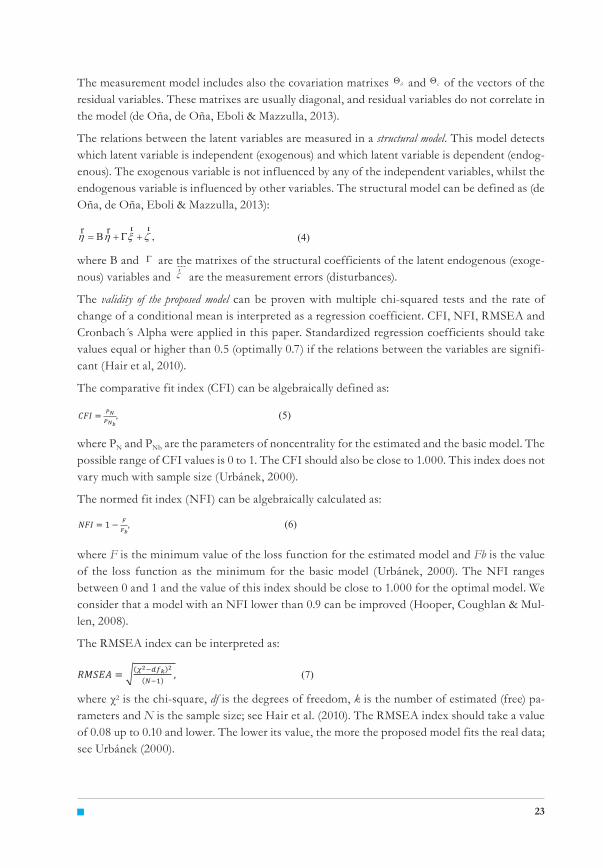
and of the vectors of the residual variables. These matrixes are usually diagonal, and residual variables do not correlate in the model (de Oña, de Oña, Eboli & Mazzulla, 2013).

The relations between the latent variables are measured in a structural model. This model detects which latent variable is independent (exogenous) and which latent variable is dependent (endog-enous). The exogenous variable is not influenced by any of the independent variables, whilst the endogenous variable is influenced by other variables. The structural model can be defined as (de Oña, de Oña, Eboli & Mazzulla, 2013):

where B and where and are the matrixes of the structural coefficients of the latent endogenous (exogenous) variables and

r are the matrixes of the structural coefficients of the latent endogenous (exoge-nous) variables and

where and are the matrixes of the structural coefficients of the latent endogenous (exogenous) variables and

r are the measurement errors (disturbances).

The validity of the proposed model can be proven with multiple chi-squared tests and the rate of change of a conditional mean is interpreted as a regression coefficient. CFI, NFI, RMSEA and Cronbach s Alpha were applied in this paper. Standardized regression coefficients should take values equal or higher than 0.5 (optimally 0.7) if the relations between the variables are signifi-cant (Hair et al, 2010).

The comparative fit index (CFI) can be algebraically defined as:

where PN and PNb are the parameters of noncentrality for the estimated and the basic model. The possible range of CFI values is 0 to 1. The CFI should also be close to 1.000. This index does not vary much with sample size (Urbánek, 2000).

The normed fit index (NFI) can be algebraically calculated as:

where F is the minimum value of the loss function for the estimated model and Fb is the value of the loss function as the minimum for the basic model (Urbánek, 2000). The NFI ranges between 0 and 1 and the value of this index should be close to 1.000 for the optimal model. We consider that a model with an NFI lower than 0.9 can be improved (Hooper, Coughlan & Mul-len, 2008).

The RMSEA index can be interpreted as:

where χ2 is the chi-square, df is the degrees of freedom, k is the number of estimated (free) pa-rameters and N is the sample size; see Hair et al. (2010). The RMSEA index should take a value of 0.08 up to 0.10 and lower. The lower its value, the more the proposed model fits the real data; see Urbánek (2000).

,r rr r

(4)

(5)

(6)

(7)

joc4-2015_v2b.indd 23 31.12.2015 13:03:51


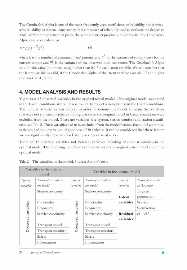
The Cronbach s Alpha is one of the most frequently used coefficients of reliability and it meas-ures reliability as internal consistency. It is a measure of reliability used to evaluate the degree to which different test items that probe the same construct produce similar results. The Cronbach s Alpha can be calculated as:

where k is the number of estimated (free) parameters, is the variance of component i for the current sample and is the variance of the observed total test scores. The Cronbach s Alpha should take value (in optimal case) higher than 0.7 for each latent variable. We can consider that the latent variable is valid, if the Cronbach s Alpha of the latent variable exceeds 0.7 and higher (Urbánek et al., 2011).

4. MODEL ANALYSIS AND RESULTSThere were 15 observed variables in the original tested model. This original model was tested in the Czech conditions at first. It was found the model is not optimal in the Czech conditions. The number of variables was reduced in order to optimise the model. It means that variables that were not statistically reliable and significant in the original model in Czech conditions were excluded from the model. These are variables fare system, station comfort and station cleanli-ness, see Tab. 2. These variables had to be excluded from the model because the model with these variables had too low values of goodness-of-fit indexes. It can be considered that these factors are not significantly important for Czech passengers’ satisfaction.

There are 12 observed variables and 15 latent variables including 12 residual variables in the optimal model. The following Tab. 2 shows the variables in the original tested model and in the optimal model.

Tab. 2 – The variables in the model. Source: Author s own.

Variables in the original model

Variables in the optimal model

Type of variable

Name of variable in the model

Type of variable


Type of variable


Obs

erve

d va

riab

les

Station proximity

Obs

erve

d va

riab

les

Station proximityLatent variables

Logistic parameters

Punctuality Punctuality ServiceFrequency Frequency SatisfactionService continuity Service continuity Residual

variablese1 – e12

Transport speed Transport speedTransport comfort Transport comfortSafety SafetyInformation Information

, (8)

joc4-2015_v2b.indd 24 31.12.2015 13:03:52

��

Obs

erve

d va

riab

les Timetable clarity

Obs

erve

d va

riab

les Timetable clarity

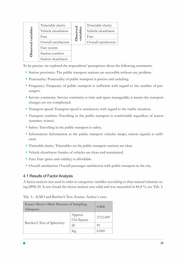
Vehicle cleanliness Vehicle cleanlinessFare FareOverall satisfaction Overall satisfactionFare systemStation comfortStation cleanliness

To be precise, we explored the respondents’ perceptions about the following statements:

Station proximity: The public transport stations are accessible without any problem.

Punctuality: Punctuality of public transport is precise and unfailing.

Frequency: Frequency of public transport is sufficient with regard to the number of pas-sengers.

Service continuity: Service continuity is time and space manageable; it means the transport changes are not complicated.

Transport speed: Transport speed is satisfactory with regard to the traffic situation.

Transport comfort: Travelling in the public transport is comfortable regardless of season (summer, winter).

Safety: Travelling in the public transport is safety.

Information: Information in the public transport vehicles (maps, station signals) is suffi-cient.

Timetable clarity: Timetables on the public transport stations are clear.

Vehicle cleanliness: Insides of vehicles are clean and maintained.

Fare: Fare (price and validity) is affordable.

Overall satisfaction: Overall passenger satisfaction with public transport in the city.

4.1 Results of Factor AnalysisA factor analysis was used in order to categorize variables according to their mutual relations us-ing SPSS 20. It was found the factor analysis was valid and was successful in 86.8 %; see Tab. 3.

Tab. 3 – KMO and Bartlett’s Test. Source: Author s own.

Kaiser-Meyer-Olkin Measure of Sampling Adequacy.

0.868

Bartlett’s Test of Sphericity

Approx. Chi-Square

2712.699

df 91Sig. 0.000

joc4-2015_v2b.indd 25 31.12.2015 13:03:52


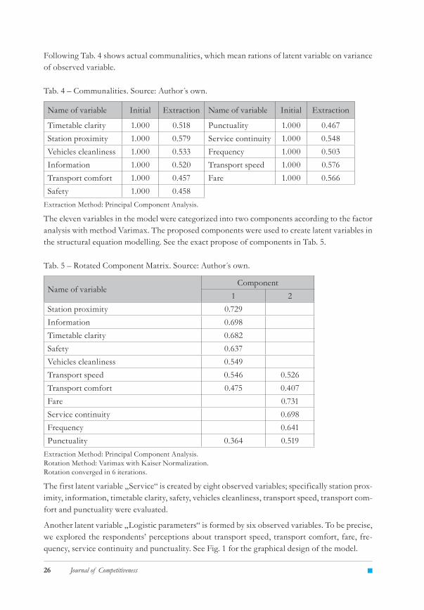
Following Tab. 4 shows actual communalities, which mean rations of latent variable on variance of observed variable.

Tab. 4 – Communalities. Source: Author s own.

Name of variable Initial Extraction Name of variable Initial Extraction

Timetable clarity 1.000 0.518 Punctuality 1.000 0.467Station proximity 1.000 0.579 Service continuity 1.000 0.548Vehicles cleanliness 1.000 0.533 Frequency 1.000 0.503Information 1.000 0.520 Transport speed 1.000 0.576Transport comfort 1.000 0.457 Fare 1.000 0.566Safety 1.000 0.458

Extraction Method: Principal Component Analysis.

The eleven variables in the model were categorized into two components according to the factor analysis with method Varimax. The proposed components were used to create latent variables in the structural equation modelling. See the exact propose of components in Tab. 5.

Tab. 5 – Rotated Component Matrix. Source: Author s own.

Name of variableComponent

1 2Station proximity 0.729Information 0.698Timetable clarity 0.682Safety 0.637Vehicles cleanliness 0.549Transport speed 0.546 0.526Transport comfort 0.475 0.407Fare 0.731Service continuity 0.698Frequency 0.641Punctuality 0.364 0.519

Extraction Method: Principal Component Analysis.Rotation Method: Varimax with Kaiser Normalization.Rotation converged in 6 iterations.

The first latent variable „Service“ is created by eight observed variables; specifically station prox-imity, information, timetable clarity, safety, vehicles cleanliness, transport speed, transport com-fort and punctuality were evaluated.

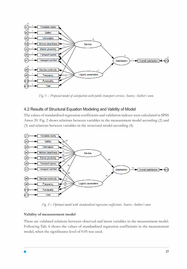
Another latent variable „Logistic parameters“ is formed by six observed variables. To be precise, we explored the respondents’ perceptions about transport speed, transport comfort, fare, fre-quency, service continuity and punctuality. See Fig. 1 for the graphical design of the model.

joc4-2015_v2b.indd 26 31.12.2015 13:03:52

��

Fig. 1 – Proposed model of satisfaction with public transport services. Source: Author s own.

4.2 Results of Structural Equation Modeling and Validity of ModelThe values of standardised regression coefficients and validation indexes were calculated in SPSS Amos 20. Fig. 2 shows relations between variables in the measurement model according (2) and (3) and relations between variables in the structural model according (4).

Fig. 2 – Optimal model with standardised regression coefficients. Source: Author s own.

Validity of measurement model

There are validated relations between observed and latent variables in the measurement model. Following Tab. 6 shows the values of standardised regression coefficients in the measurement model, when the significance level of 0.05 was used.

joc4-2015_v2b.indd 27 31.12.2015 13:03:52


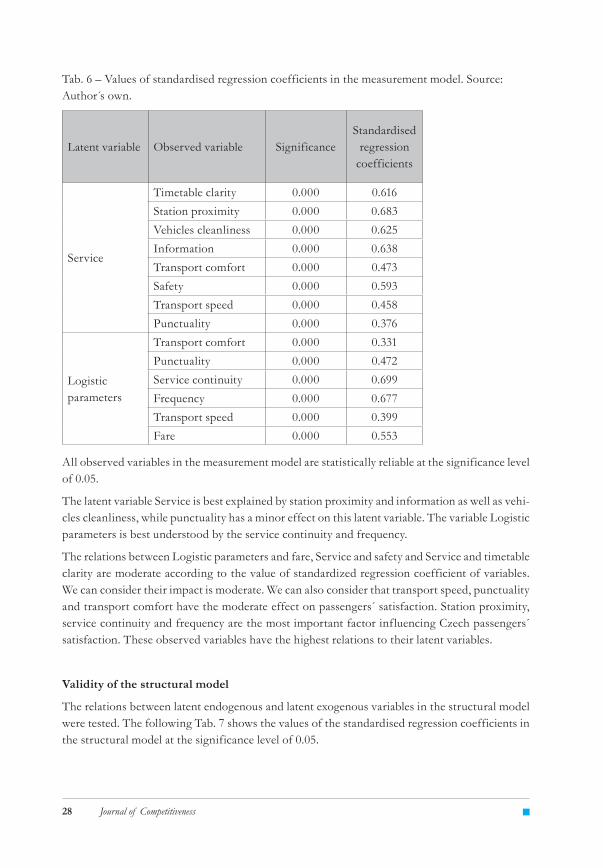
Tab. 6 – Values of standardised regression coefficients in the measurement model. Source: Author s own.

Latent variable Observed variable SignificanceStandardised

regression coefficients

Service

Timetable clarity 0.000 0.616Station proximity 0.000 0.683Vehicles cleanliness 0.000 0.625Information 0.000 0.638Transport comfort 0.000 0.473Safety 0.000 0.593Transport speed 0.000 0.458Punctuality 0.000 0.376

Logistic parameters

Transport comfort 0.000 0.331Punctuality 0.000 0.472Service continuity 0.000 0.699Frequency 0.000 0.677Transport speed 0.000 0.399Fare 0.000 0.553

All observed variables in the measurement model are statistically reliable at the significance level of 0.05.

The latent variable Service is best explained by station proximity and information as well as vehi-cles cleanliness, while punctuality has a minor effect on this latent variable. The variable Logistic parameters is best understood by the service continuity and frequency.

The relations between Logistic parameters and fare, Service and safety and Service and timetable clarity are moderate according to the value of standardized regression coefficient of variables. We can consider their impact is moderate. We can also consider that transport speed, punctuality and transport comfort have the moderate effect on passengers´ satisfaction. Station proximity, service continuity and frequency are the most important factor influencing Czech passengers´ satisfaction. These observed variables have the highest relations to their latent variables.

Validity of the structural model

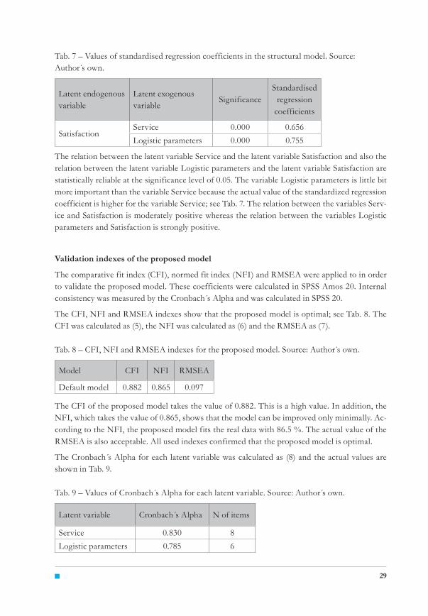
The relations between latent endogenous and latent exogenous variables in the structural model were tested. The following Tab. 7 shows the values of the standardised regression coefficients in the structural model at the significance level of 0.05.

joc4-2015_v2b.indd 28 31.12.2015 13:03:52

��

Tab. 7 – Values of standardised regression coefficients in the structural model. Source: Author s own.

Latent endogenous variable

Latent exogenous variable

SignificanceStandardised

regression coefficients

SatisfactionService 0.000 0.656Logistic parameters 0.000 0.755

The relation between the latent variable Service and the latent variable Satisfaction and also the relation between the latent variable Logistic parameters and the latent variable Satisfaction are statistically reliable at the significance level of 0.05. The variable Logistic parameters is little bit more important than the variable Service because the actual value of the standardized regression coefficient is higher for the variable Service; see Tab. 7. The relation between the variables Serv-ice and Satisfaction is moderately positive whereas the relation between the variables Logistic parameters and Satisfaction is strongly positive.

Validation indexes of the proposed model

The comparative fit index (CFI), normed fit index (NFI) and RMSEA were applied to in order to validate the proposed model. These coefficients were calculated in SPSS Amos 20. Internal consistency was measured by the Cronbach s Alpha and was calculated in SPSS 20.

The CFI, NFI and RMSEA indexes show that the proposed model is optimal; see Tab. 8. The CFI was calculated as (5), the NFI was calculated as (6) and the RMSEA as (7).

Tab. 8 – CFI, NFI and RMSEA indexes for the proposed model. Source: Author s own.

Model CFI NFI RMSEA

Default model 0.882 0.865 0.097

The CFI of the proposed model takes the value of 0.882. This is a high value. In addition, the NFI, which takes the value of 0.865, shows that the model can be improved only minimally. Ac-cording to the NFI, the proposed model fits the real data with 86.5 %. The actual value of the RMSEA is also acceptable. All used indexes confirmed that the proposed model is optimal.

The Cronbach s Alpha for each latent variable was calculated as (8) and the actual values are shown in Tab. 9.

Tab. 9 – Values of Cronbach s Alpha for each latent variable. Source: Author s own.

Latent variable Cronbach s Alpha N of items

Service 0.830 8Logistic parameters 0.785 6

joc4-2015_v2b.indd 29 31.12.2015 13:03:52

Journal of Competitiveness �0

It was find that all latent variables are valid because the value of Cronbach s Alpha for each latent variable is higher than 0.7. It is possible to determine this model is valid.

5. DISCUSSION AND MANAGERIAL IMPLICATIONSAccording to results of this research it is possible to state that Czech passengers’ satisfaction with public transport is affected the most by logistic parameters. It was found station proximity, service continuity and frequency are the most important indicators of satisfaction. According to de Oña, de Oña, Eboli and Mazzulla (2013) Czech passengers agree with other European pas-sengers that service frequency is very important, but Czech passengers do not agree with other European passengers in their opinions about low importance of station proximity. Whereas sta-tion proximity is not so important factor of satisfaction for other passengers, it is very important factor for Czech passengers. Whereas other European passengers claim that transport speed is very important, transport speed is not so important for Czech passengers. Czech passengers require service continuity, but they don t take care so much about fare and safety. Czech pas-sengers also don t require courtesy and professionalism of staff like other European passengers. This difference could originate from Czech system of public city transport when majority of passengers don t come into contact with drivers. Czech passengers expect that their orientation during travelling is easy, so the information in the public transport vehicles has to be sufficient.

In the future research in this area it is possible to extend the factors of comfort and personal factors. It can be suggested to find the opinions of passengers about temperature in the vehicles in summer and in winter, accessibility of vehicles or space in vehicles and also about safe driving of vehicles.

It can be recommended to the management of public transport service to improve logistic fac-tors of transport such as number of vehicles, frequency and service continuity to attract more passengers. The management has to keep in mind that Czech passenger has to feel comfortable and well-informed during travelling. Implementation of these suggestions should lead to the decrease in the number of cars in cities, to the reduction of the environment pollution and also the noise abatement.

6. CONCLUSIONThis paper focuses on the factors affecting passengers´ satisfaction with public transport in the Czech Republic. The aim of this paper was to quantify factors and identify the most important factors influencing customer satisfaction with public transport services in the Czech Republic. A factor analysis with method Varimax was used in order to categorize variables according to their mutual relations. A structural equation modelling was used to evaluate the proposed model and find the optimal model with the most significant factors. The theoretical background of these methods is also the part of this paper. The data that were analysed came from questioning. CFI, RMSEA, NFI and Cronbach s Alpha were used to validate the rate in which the proposed model fits the real data.

This research demonstrated that factor analysis and structural equation modelling methodology is a powerful tool which can be used as a technique to identify the latent aspects that are hidden

joc4-2015_v2b.indd 30 31.12.2015 13:03:52

�1

under a series of attributes describing the quality of the service. This type of methodology is use-ful, but it is difficult to establish if this tool is better than other methodologies. According to the goodness-of-fit indexes used, the proposed model can be considered to be optimal for describing of behaviour of Czech passengers. The fit of the real data with the proposed model is high.

AknowledgementThis paper was created within the project SGS Nákupní chování Generace Y v mezinárodním kontextu, project registration number SP2015/118 and was supported within Operational Programme Education for Competiti-veness – Project No. CZ.1.07/2.3.00/20.0296.

ReferencesAntonucci, L. et al. (2014). Passenger satisfaction: A multi-group analysis. Quality and Quantity, 48(1), 337-345. doi: 10.1007/s11135-012-9771-7

de Oña, J., de Oña, R., Eboli L., & Mazzulla, G. (2013). Perceived service quality in bus transit service: A structural equation approach. Transport Policy, 29, 219-226. doi:10.1016/j.tranpol.2013.07.001

de Oña, J., de Oña, R., & Calvo, F. J. (2012). A classification tree approach to identify key factors of transit service quality. Expert Systems With Applications, 39(12), 11164-11171. doi:10.1016/j.eswa.2012.03.037

Hair, J. F. et al. (2010). Multivariate Data Analysis (7th ed.). Upper Saddle River, New Jersey: Prentice Hall.

Hendl, J. (2004). Přehled statistických metod z pracování dat. Praha: Portál.

Hooper, D., Coughlan, J., & Mullen, M. R. (2008). Structural Equation Modelling: Guidelines for Determining Model Fit. Electronic Journal Of Business Research Methods, 6(1), 53-59.

Malhotra, N. K., & Birks, D. F. (2006). Marketing Research. An Applied Approch (2nd ed.). London: Prentice Hall.

Meloun, M., Militký, J., & Hill, M. (2005). Počítačová analýza vícerozměrných dat v příkladech. Praha: Academia.

Mouwen A. (2015). Drivers of Customer Satisfaction with Public Transport Services. Transportation Research: Part A: Policy And Practice [serial online], 78, 1-20. doi:10.1016/j.tra.2015.05.005

Nachtigall, C. et al. (2003). (Why) Should We Use SEM? Pros and Cons of Structural Equation Modelling. Methods of Psychological Research Online, 8(2), 1-22. Retrieved from Deutsche Gesellschaft für Psychologie e.V., DGPs., from http://www.dgps.de/fachgruppen/methoden/mpr-online/issue20/art1/mpr127_11.pdf

Pecáková, I. (2008). Statistika v terénních průzkumech. Praha: Professional Publishing.

Replogle, M. A., & Fulton, L. (2014). A Global High Shift Scenario: Impacts And Potential For More Public Transport, Walking, And Cycling With Lower Car Use. New York: Institute for Transportation and Development Policy (ITDP). Retrieved from: http://www.itdp.org/wp-content/uploads/2014/09/A-Global-High-Shift-Scenario_WEB1.pdf

1.

2.

3.

4.

5.

6.

7.

8.

9.

10.

11.

12.

joc4-2015_v2b.indd 31 31.12.2015 13:03:53


Shiau, W., & Luo, M. M. (2012). Factors affecting online group buying intention and satisfaction: A social exchange theory perspective. Computers In Human Behavior, 28(6), 2431-2444. doi:10.1016/j.chb.2012.07.030

Urbánek, T. et al. (2011). Psychometrika: Měření v psychologii. Praha: Portál.

Urbánek, T. (2000). Strukturální modelování v psychologii. Brno: Psychologický ústav AV ČR a Nakladatelství Pavel Křepela.

Weinstein, A. (2000). Customer satisfaction among transit riders: How customers rank the relative importance of various service attributes. Transportation Research Record, 1735, 123-132. doi: 10.3141/1735-15

Zamazalová, M. (2009). Marketing obchodní firmy. Praha: Grada.

Contact informationIng. Pavlína PawlasováVysoká škola báňská – Technická univerzita Ostrava, Faculty of EconomicsSokolská třída 33, 701 21 Ostrava, Czech RepublicE-mail: [email protected]

13.

14.

15.

16.

17.

joc4-2015_v2b.indd 32 31.12.2015 13:03:53

The Factors Influencing Satisfaction with Public City ... · The Factors Influencing Satisfaction...

Documents

Transcript of The Factors Influencing Satisfaction with Public City ... · The Factors Influencing Satisfaction...