The Facility Location Problem with Bernoulli Demands

Maria Albareda-Sambolaa, Elena Fernandezb∗, Francisco Saldanha-da-Gamac

a Universitat Politecnica de Catalunya, Dept. d’Estadıstica i Investigacio Operativa,Carrer Colom, 11, 08022 Terrassa, Spain

b Universitat Politecnica de Catalunya, Dept. d’Estadıstica i Investigacio Operativa,Campus Nord, C5-208, Jordi Girona 1–3, 08034 Barcelona, Spain

c Universidade de Lisboa, Faculdade de Ciencias, Dept. Estatıstica e Investigacao Operacional eCentro de Investigacao Operacional,

Bloco C6, Piso 4, 1749-016 Lisboa, Portugal

July 30, 2008

Abstract

In this paper we address a discrete capacitated facility location problem in which customers haveBernoulli demands. The problem is formulated as a two-stage stochastic program. The goal is to definean a priori solution for the location of the facilities and for the allocation of customers to the operatingfacilities that minimize the expected value of the recourse function. A closed form is presented for therecourse function and an approximation is proposed for situations in which it can not be evaluatedexactly. The stochastic assignment problem resulting from setting the operating facilities is studiedand a procedure is proposed to approximate its optimal solution. We formulate the capacitated facilitylocation problem with Bernoulli demands under perfect information and, finally, we propose a heuristicto find an a priori solution. Computational results are presented for the homogeneous case.

1 Introduction

A Facility Location Problem looks for the best location for a set of facilities that must satisfy requestsof service coming from a given set of customers. Often it is assumed that customers demands of serviceare part of the input data of the problem and, thus, are known in advance. However, it is well-knownthat in practice this very seldom occurs, since usually there is a high level of uncertainty associatedwith the demand. Typical examples of location problems with non-deterministic demands include notonly the location of emergency facilities, but also any location problem where the demand levels mightchange over different time periods (postal services, super-markets, warehouses to distribute goods withseasonal-dependent demand, airports, etc.) Brandeau and Chiu [9], Louveaux [23] and Snyder [28] havesurveyed different aspects of Stochastic Location Problems.

There are several alternatives for handling problems that exhibit uncertainty in service demands. Ifno assumption is made on the probability distribution of the demands, one possibility is to guarantee therobustness of the obtained solutions by taking into account several possible scenarios. Depending on thecontext, robustness can be evaluated by means of different measures like, for instance, the minimizationof the cost associated with the most adverse scenario or the minimization of the cost associated with themost likely scenario. Some related references are, for instance, Averbakh and Berman [3, 4, 5], Carrizosaand Nickel [11], or Conde [12, 13]. Other possibilities arise when the stochastic nature of the demandsis captured by means of some assumption on their probability distribution. For instance, when servicerequests that arrive when the servers are busy are rejected, some authors have considered probabilisticconstraints to guarantee that the probability that customers with demand receive the requested serviceis above a certain threshold (e.g. ReVelle [26] and Toregas et al. [29]). From a different point of view,when it is accepted that requests that arrive when servers are busy can wait until some server is free,queueing-location models address the minimization of the expected waiting time in the queue or theexpected length of the queue. Some references along this line are Marianov and ReVelle [25], Carrizosa

∗Corresponding author. e-mail address: e.fernandez@upc.edu

1

et al. [10], or Fernandez et al. [15]. A different methodology to handle these problems comes fromStochastic Programming. One possibility is to define a recourse function that, given an a priori solution,indicates the best decision to make for each possible realization of the random vector, and then to find thea priori solution that minimizes the expected cost of this recourse function. Louveaux and Peeters [24]and Laporte et al. [22] explore this possibility for the Uncapacitated Facility Location Problem. In bothpapers, a set of scenarios is considered each of which occurring with some specified probability. Riis andAndersen [27] study a capacity expansion problem arising in telecommunication networks that involvesno location decisions. The authors consider the realistic situation in which demand is uncertain andfollows some known probability distribution. A stochastic integer programming formulation is proposedfor the problem.

Frequently, the request of service of a given customer is expressed in terms of a “quantity” thatrepresents the amount of resources of a service center that will be consumed if the customer is served.Nevertheless, in many situations requests for service are unitary in the sense that some service is requestedthat requires one unit of resource (e.g. one worker) from the service center. In such situation, each possiblescenario is characterized by the set of customers with demand. This is, for instance, the case when serversare repairmen and requests of service from customers correspond to requests for repairing. Now, requestscan be modeled by means of binary vectors. In this context, if demands are stochastic, the componentsof such a vector are 0-1 random variables. In this paper we consider the particular case in which the 0-1random variables are independent and follow a Bernoulli probability distribution.

The facility location problem that we address in this paper is stated in a discrete setting. Accordingly,we assume that there is a finite set of potential locations for the facilities. Moreover, each customer mustbe assigned to one single facility. The decision regarding where to locate the facilities and how to allocatethe customers to the operating facilities must be made before knowing which customers will in fact requestthe service. Actually, depending on the context, locational and assignment decisions are often made ona strategic or tactical level due to the resources that may have to be allocated to the implementation ofthese decisions (e.g. financial resources or human workforce). Therefore, not only it is not desirable tochange these decisions too often but also, such decisions are often made and implemented before knowingexactly how the future will be, for instance, in terms of the potential demand. In this case, the planningmust be ready before all requests for the service are received (see Snyder [28] for a deeper discussion onthese aspects).

We assume that each facility has a capacity that represents the maximum number of customersthat can be served from it (in case it is operating). Thus, in some realizations, there might be morecustomers allocated to one operating facility than the capacity of the facility. In such situation, if thereare more customers requesting the service than the capacity of the facility to which they are allocated,some customers can not be served and a penalty cost is incurred for each request declined. We alsoconsider the situation in which a facility can only be installed if a pre-specified minimum number ofdemand points is assigned to it. It should be noted that often, this imposition is not drawn by the costsbut by preliminary decisions made to assure a somehow balanced system. This requirement is quitegeneral, since the situation in which no such limits exist becomes a particular case of the problem we arestudying. The goal is to decide where to locate the facilities and how to allocate all the customers so as tominimize the overall expected cost which, in addition to the penalty cost above mentioned also includesthe costs for installing the facilities and the demand satisfaction costs. This is a Stochastic CombinatorialOptimization Problem, in which the stochasticity is associated with the customers demands, which weassume to follow a Bernoulli distribution.

Several Stochastic Combinatorial Optimization Problems with Bernoulli demands have been addressedin the literature in the context of the minimization of a recourse function. This is the case of theprobabilistic travelling salesman problem. Jaillet [19] introduces this problem and presents a closedform expression for computing efficiently the expected value of the length of any given tour. Laporteet al. [21] propose a linear stochastic program model that is solved using a branch-and-cut approach.More recently, Bianchi and Campbell [7] propose a heuristic approach for the problem. The reader isreferred to this latter work for additional references on this problem. Berman and Simchi-Levi [6] studya single-vehicle location-routing problem with Bernoulli demands. The authors formulate the problemand develop a lower bound on the value of the optimal a priori tour. Quite recently, Albareda-Sambola

2

et al. [1] addressed a study of location-routing problems with Bernoulli demands. The authors proposeheuristics and lower bounds to minimize the expected value of the defined recourse function. Albareda-Sambola et al. [2] propose an exact algorithm for minimizing the expectation of a recourse function forthe Stochastic Generalized Assignment Problem, where it is assumed that the customers demands followa Bernoulli distribution. To the best of our knowledge, no work exists in the literature that uses a similarmethodology for discrete location problems with Bernoulli demands.

In this paper the optimization of the above described Facility Location Problem with Bernoulli De-mands (FLPBD) is studied. In the next section the problem is formally described and a recourse functionis presented that allows the FLPBD to be formulated as a two-stage stochastic program. The goal is tofind an a priori solution that minimizes the expected cost of the recourse function. A closed expressionfor this function is derived, which is simple to evaluate in the homogeneous situation (all customershave demand with the same probability). Since its evaluation becomes unaffordable as the number ofcustomers increases, the general case is addressed in Subsection 2.1, in which an approximation of therecourse function is proposed. Like in most location problems, the assignment subproblem to be solvedwhen the set of facilities to open is known is of interest on its own. In Section 3 a formulation is presentedfor this stochastic problem and a solution algorithm is proposed which is based on the resolution of aminimum cost flow problem in an auxiliary network. The problem under perfect information that resultsfor a particular a realization of the random vector is addressed in Section 4. This problem is indeedclosely related to the FLPBD and is also of great interest, since its resolution for a large sample of real-izations of the random vector gives us valuable information for evaluating the solutions obtained for theoverall stochastic problem. Feasible solutions are obtained with a heuristic procedure that is proposedin Section 5. Section 6 is devoted to the computational experience performed to evaluate the proposedmethodologies. The paper ends with some conclusions and suggestions for further research.

2 Definition of the problem

Let I and J denote the set of indices for the potential locations of facilities and for customers, respectively.Let n = |J |. We assume that the demand of service of each customer j ∈ J is given by a binary randomvariable, that we denote by ξj , indicating whether or not customer j has demand. We further assumethat ξj follows a Bernoulli probability distribution of parameter pj . For i ∈ I, we consider, in addition,the following notation:

fi Fixed set-up cost for opening facility i;`i Minimum number of customers that have to be assigned to facility i if it is opened;Ki Maximum number of customers that can be served from facility i when it is opened;cij Cost for serving customer j from facility i (j ∈ J).

It should be noted that for a realization of the random vector not all the customers need to havedemand. For this reason, we distinguish between the assignment of customers to plants, which is donea priori and is independent of the potential realizations, and the service of customers from open plants,which is decided a posteriori, once the realization is known. Thus, an a priori solution is given by a set ofoperating facilities together with an assignment of all the customers to these facilities, such that for anyopen plant the set of customers that are assigned to it is at least `i. Observe that Ki is an upper boundon the number of customers that can be served from an opened plant and, thus, this is not taken intoaccount for the feasibility of a priori solutions. Let Ji denote the set of customers assigned to facility iin the a priori solution, with zi = |Ji|. Throughout the text the customers with demand in a potentialrealization are referred to as the demand customers. Also, for a potential realization, ηi denotes thenumber of demand customers assigned to facility i.

Given an a priori solution, the a posteriori solution indicates the decisions to make, once demandcustomers are known. If the number of customers assigned to an open facility i does not exceed its upperbound, i.e. zi ≤ Ki, then in the a posteriori solution all the demand customers indexed in Ji receiveservice from plant i. However, when the number zi exceeds Ki, if ηi is also greater than Ki then the aposteriori solution consists of randomly selecting Ki demand customers from Ji for being actually servedfrom plant i. Each of the remaining (ηi −Ki) demand customers remain unserved. A service cost cij is

3

incurred for each served customer j. A penalty cost that we denote by g is incurred for every unservedcustomer. The recourse function is the expected cost, over all possible realizations of the demand vectorand all realizations of the random choices for resolving the excess demand in plants, of the a posteriorisolution.

The FLPBD consists of finding a set of facilities to open and an allocation of the customers to theopened facilities, in such a way that the sum of the fixed cost associated with the open facilities andthe recourse function is minimized. In order to give a mathematical programming formulation for thisproblem, we consider the following sets of decision variables:

yi ={

1 if a facility is established at i0 otherwise

(i ∈ I)

xij ={

1 if customer j is allocated to facility i0 otherwise

(i ∈ I, j ∈ J)

The FLPBD can be formulated as follows:

(P ) min∑i∈I

fiyi + Eξ(Service cost + Penalty cost) (1)

s. t.∑i∈I

xij = 1 j ∈ J (2)

xij ≤ yi i ∈ I, j ∈ J (3)

`iyi ≤∑j∈J

xij i ∈ I, j ∈ J (4)

yi ∈ {0, 1} i ∈ I (5)xij ∈ {0, 1} i ∈ I, j ∈ J (6)

As mentioned above, the objective function (1) includes the fixed costs for opening the facilities andthe recourse function. Constraints (2) assure that all customers will be assigned to (exactly) one facilitywhile constraints (3) assure that this assignments can only be done to operating facilities. Constraints(4) state the minimum number of customers that should be assigned to one operating facility. Finally,constraints (5) and (6) are domain constraints.

We next analyze in more detail the recourse function. To do so, for a given solution, (y, x), we expressboth zi and ηi in terms of the decision variables. That is

zi =∑j∈J

xij and ηi =∑j∈J

ξjxij

In addition, define generically Pi(s) as the conditional probability of serving a demand customerassigned to facility i ∈ I given that the total number of demand customers assigned to facility i is s (i.e.ηi = s). For i ∈ I, we have:

Pi(s) =min{Ki, s}

s={

1 if s ≤ KiKis otherwise

For a given a priori solution we can, thus, evaluate its recourse function. Therefore, we can write:

Eξ(Service cost + Penalty cost)

=∑i∈I

zi∑s=0

P[ηi = s]× E[Service cost + penalty cost|ηi = s]

=∑i∈I

Ki∑s=0

P[ηi = s]× E[Service cost|ηi = s]

+∑i∈I

zi∑s=Ki+1

P[ηi = s]× E[Service cost + penalty cost|ηi = s]

4

=∑i∈I

Ki∑s=0

P[ηi = s]∑j∈J

P[ξj = 1|ηi = s]cijxij

+∑i∈I

zi∑s=Ki+1

P[ηi = s]

∑j∈J

P[ξj = 1|ηi = s]Pi(s)cijxij + g(s−Ki)

=∑i∈I

zi∑s=0

P[ηi = s]∑j∈J

P[ξj = 1|ηi = s]Pi(s)cijxij

+∑i∈I

g

zi∑s=Ki+1

P[ηi = s](s−Ki)

=∑i∈I

zi∑s=0

P[ηi = s]∑j∈J

P[ξj = 1|ηi = s]min{Ki, s}

scijxij

+ g

∑i∈I

zi∑s=Ki+1

P[ηi = s](s−Ki)

Thus, the objective function (1) becomes

∑i∈I

fiyi +∑i∈I

zi∑s=0

P[ηi = s]∑j∈J

P[ξj = 1|ηi = s]min{Ki, s}

scijxij

+ g

∑i∈I

zi∑s=Ki+1

P[ηi = s](s−Ki)

In the general case, when the probabilities pj are not necessarily equal for all customers, the probabilitydistribution of the ηi variables is quite involved. For a given solution (y, x) recall that Ji = {j ∈ J : xij =1}. Then,

P[ηi = s] =∑

S⊂Ji:|S|=s

∏j∈S

pj

∏j′ /∈S

(1− pj′) (7)

=1s

∑j∈Ji

pjP[ηi − ξj = s− 1]

= · · ·

=1s!

∑j1∈Ji

pj1

∑j2∈Ji\{j1}

pj2 · · ·∑

js∈Ji\{j1,...,js−1}

pjs

∏j 6=j1,j2,...,js

(1− pj)

.

However, when pj = p ∀j ∈ J , ηi is a Binomial random variable with parameters zi and p. Thus,P[ηi = s] =

(zis

)ps(1−p)zi−s, s = 0, . . . , zi. In this case, taking into account that (ηi − 1)|(ξj=1) ∼ Bin(zi − 1, p),

we have:

P[ξj = 1|ηi=s] =P[ηi = s|ξj = 1]P[ξj = 1]

P[ηi = s]=

P[ηi − 1 = s− 1||ξj = 1]P[ξj = 1]

P[ηi = s]

=

(zi−1s−1

)ps(1− p)zi−sp(

zis

)ps(1− p)zi−s

=s

zi.

and we obtain the following closed expression for the objective function:

5

∑i∈I

fiyi +∑i∈I

zi∑s=0

(zi

s

)ps(1− p)zi−s min{Ki, s}

zi

∑j∈J

cijxij

+∑i∈I

g

zi∑s=Ki+1

((zi

s

)ps(1− p)zi−s(s−Ki)

) . (8)

2.1 Normal approximation for the probability distribution of total demand for openplants.

The evaluation of the expression (7) becomes unaffordable as zi increases. However, for values of zi largeenough, the central limit theorem allows us to approximate the distribution of ηi by a normal law.

Indeed, since the expected value of ηi is µi =∑

j∈Ji

pj , and its variance, σ2i =

∑j∈Ji

pj(1− pj), we have

ηi − µi

σi≈ N (0, 1) .

In addition, for a fixed j ∈ Ji, let ηji =

∑k∈Ji\j

ξk. Then

E[ηji ] =

∑k∈Ji\j

pk = µji ;

andvar[ηj

i ] =∑

k∈Ji\j

pk(1− pk) = σji .

Thus, we also haveηj

i − µji

σji

≈ N (0, 1) .

For a given solution to problem P, (y, x), we denote by I the index set of opened facilities.

Proposition 1 Let (y, x) be a solution to problem P. Then, for all i ∈ I and j ∈ Ji,

P[ξj = 1|ηi = s] ∼αj

i (s)αi(s)

pj ,

where

αi(s) = Φ(

s + 0.5− µi

σi

)− Φ

(s− 0.5− µi

σi

),

and

αji (s) = Φ

(s− 1 + 0.5− µj

i

σji

)− Φ

(s− 1− 0.5− µj

i

σji

).

Proof:

P[ξj = 1|ηi = s] =P[ηi = s|ξj = 1]P[ξj = 1]

P[ηi = s].

6

We have,

P[ηi = s] = P[ηi − µi

σi=

s− µi

σi

]≈ Φ

(s + 0.5− µi

σi

)− Φ

(s− 0.5− µi

σi

)= αi(s).

Also,

P[ηi = s|ξj = 1] = P[ηji = s− 1]

= P

[ηj

i − µji

σji

=s− 1− µj

i

σji

]

≈ Φ

(s− 1 + 0.5− µj

i

σji

)− Φ

(s− 1− 0.5− µj

i

σji

)= αj

i (s).

Therefore,

P[ξj = 1|ηi = s] =αj

i (s)αi(s)

pj , and the result follows.

�

Proposition 2 For any solution (y, x) to formulation P for which zi is large enough, for all i ∈ I, theobjective function can be approximated by

∑i∈I

fiyi +∑i∈I

∑j∈J

(cijxijpj

zi∑s=0

min{Ki, s}s

αji (s)

)+ g

∑i∈I

zi∑s=Ki+1

αi(s)(s−Ki).

Proof: The result holds by Proposition 1 since

∑i∈I

fiyi +∑i∈I

zi∑s=0

P[ηi = s]∑j∈J

P[ξj = 1|ηi = s]min{Ki, s}

scijxij

+ g

∑i∈I

zi∑s=Ki+1

[P[ηi = s](s−Ki)]

=∑i∈I

fiyi +∑i∈I

zi∑s=0

αi(s)∑j∈J

αji (s)

αi(s)pj

min{Ki, s}s

cijxij

+ g

∑i∈I

zi∑s=Ki+1

αi(s)(s−Ki)

�

3 The Stochastic Assignment Subproblem

In this section we address the assignment problem that results when the set of operating facilities isknown. Let I ⊂ I denote the set of facilities that are opened and assume that

∑i∈bI `i ≤ |J |, to guarantee

7

that there exists a feasible assignment on set J . We want to find an assignment of customers within theset of open facilities of minimum expected cost. This problem can be expressed as:

(AP (I)) min∑i∈bI

zi∑s=0

P[ηi = s]∑j∈J

P[ξj = 1|ηi = s]min{Ki, s}

scijxij

+g∑i∈bI

zi∑s=Ki+1

P[ηi = s](s−Ki) (9)

s. t.∑i∈bI

xij = 1 ∀ j ∈ J (10)

`i ≤∑j∈J

xij ∀ i ∈ I (11)

xij ∈ {0, 1} ∀ i ∈ I , j ∈ J (12)

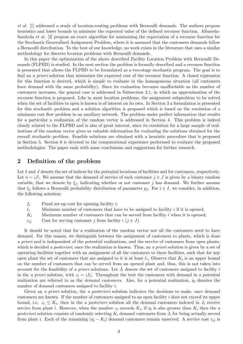
For a given set of operating facilities I it is not a simple task to solve AP (I) optimally. For this reasonwe propose a method for obtaining good quality solutions to the problem by solving a deterministicminimum cost flow problem in an auxiliary network N(I) = (V,A) defined as follows:

• The set V has a vertex associated with each customer j ∈ J , two vertices associated with each openfacility i ∈ I, and one additional vertex, that we denote v0. Let us denote V = {vr : r ∈ R}, whereR = {J} ∪ I ∪ I ′ ∪ {0}, being I ′ a copy of the set of indices of the facilities in I.

• The set of arcs contains arcs (vj , vi), ∀j ∈ J,∀i ∈ I; arcs (vi, vi′), where i ∈ I, i′ ∈ I ′ and vi′ is thecopy of vertex vi; and arcs (vi′ , v0), ∀i′ ∈ I ′.

• The vector of productions/demands b = (br)r∈R is defined as follows: all vertices vj , j ∈ J areproduction ones with bj = 1. Vertices vi, i ∈ I, are transhipment ones, i.e., bi = 0, i ∈ I. Theremaining vertices are demand ones: bi′ = `i, ∀i ∈ I and b0 = n −

∑i∈bI `i (recall that n = |J |).

Thus, network N is balanced.

• Given the above productions and demands, the flows through arcs (vj , vi) will only take values 0 or1, ∀j ∈ J, i ∈ I. They will take value 1 to represent that customer j is assigned to plant i. Thus,the flow through arcs (vi, vi′) will represent the number of customers allocated to facility i.

• Arcs (vi, vi′), i ∈ I, have a maximum capacity ui = max

{Ki,

np

KiPt∈bI Kt

}, where p denotes the average

of all pj , j ∈ J . The remaining arcs have no upper limit on their maximum flow. The rationalebehind the previous expression is to choose auxiliary capacities large enough to allow to assign allthe customers to the set I, and proportional to the service capacities, Ki.

• We define a cost function c on the arcs such that all arcs have cost zero apart from the arcs (vj , vi),whose cost is cji = cij

pj

Ki.

Figure 1 depicts a general network built as described above. Note that the solution to the minimumcost flow problem in the above network gives the optimal solution to the assignment problem when thecapacities of the facilities, Ki (i ∈ I) are so high that the capacity constraints on the plants are neverbinding. In the general case, the cost function c weights the original assignment costs penalizing assign-ments to facilities with small capacities, and giving more weight to customers with higher probability ofrequesting the service.

4 The FLPBD under perfect information

In this section we study the FLPBD under perfect information. That is, we study the problem thatresults from a particular realization of the random vector, which is the same as to consider that we

8

1

i

1

1

1

1

1

1

0

l1

li

customers plantsdummy

sinkplantsrep.

1'

i'(0,ui)

(0,∞)

(ĉij,∞)

n - Σli

(cost, capacity)

j

n

Figure 1: Auxiliary network to obtain an approximate solution to AP (I).

know in advance which customers will in fact request the service. We next study how to find an optimalsolution of the problem for each realization of the random vector. By solving such a problem for allpossible realizations of the random vector we obtain a population of optimal values, each of which withsome probability. Finding this population and its corresponding probability distribution is known inthe literature as the distribution problem (see for instance, Birge and Louveaux [8]). In particular, themean value of the above mentioned distribution gives the so-called wait-and-see value. In practice, ingeneral, it is very difficult to find the exact distribution of the above mentioned population as well asthe wait-and-see value. This is also true for the particular case of the FLPBD. However, the possibilityof solving the problem under perfect information allows us to estimate this latter value, for instance, bysimulation. By estimating the wait-and-see value we get a way for measuring the degree of stochasticityof a particular instance although, as pointed out in Birge and Louveaux [8] no such measure is absolutefor evaluating how stochastic an instance is.

In the FLPBD, a realization of the customers demands is not enough to define perfect information.Given that the number of customers with demand assigned to an open facility i may exceed its capacityKi, and given that the number of customers that can be served from facility i cannot exceed Ki, forhaving perfect information we also need to know the criterion according to which we decide whether ofnot a customer with demand is going to be served. In this paper we assume that we use a first come firstserve policy. Hence, perfect information is given by both the set of customers that have demand and alsothe order in which requests of service “arrive” at the system.

For a given realization ξ, denote by Jξ = {j ∈ J : ξj = 1} the set of indices of demand customers,nξ = |Jξ|, and by (π(1), . . . , π(nξ)) the order by which their requests of service arrive, so that π(q) is theindex of the customer corresponding to the q-th request for service, q = 1, . . . , nξ. For formulating theFLPBD under perfect information, in addition to the y variables, that represent the location decisions,and the x variables, that represent a priori assignments of customers, we define a new set of variables,denoted w, that represent the served customers in the a posteriori solution, i.e. the demand customersthat are actually served in the solution to the problem.

wij ={

1 if customer j is served from facility i0 otherwise

(i ∈ I, j ∈ Jξ)

9

The problem under perfect information can then be formulated as follows:

(PI(ξ, π)) min∑i∈I

fiyi +∑i∈I

∑j∈Jξ

cijwij + g∑j∈Jξ

(1−

∑i∈I

wij

)(13)

s. to:∑i∈I

xij = 1 j ∈ J (14)

xij 6 yj i ∈ I, j ∈ J (15)∑j∈Jξ

wij 6 Ki i ∈ I (16)

wij 6 xij i ∈ I, j ∈ Jξ (17)

`iyi 6∑j∈J

xij i ∈ I (18)

wiπ(s) − wiπ(r) 6 2− xiπ(r) − xiπ(s) i ∈ I, r < s ∈ {1, . . . , nξ} (19)

yi, wij ∈ {0, 1} i ∈ I, j ∈ Jξ (20)xij ∈ {0, 1} i ∈ I, j ∈ J (21)

In this formulation, constraints (14) and (15) together force each customer to be assigned to anoperating facility. Constraints (16) state the service capacity of each plant, and constraints (18) avoidopening a plant that does not have enough customers assigned to it. Constraints (17) ensure that servicesare provided according to the assignment of customers to plants. Finally, constraints (19) assure that ineach plant, a first call first serve policy is used to decide which customers to serve.

As mentioned before, having formulated the problem under perfect information it is possible toestimate the wait-and-see value, which is the expected value of PI(ξ, π). To do so one possibility is tosimulate the uncertain data, namely the customers that in fact have demand as well as the order bywhich they call to be served and to solve model PI(ξ, π) with some general purpose software. By doingso for several simulations and by evaluating the average of the values obtained, we get an estimate of thewait-and-see value. The difference between the value of the best solution known for P and this estimategives us an estimate of the expected value of perfect information.

5 A heuristic procedure

As mentioned in the previous section, one advantage of formulating the problem under perfect informa-tion (13)-(21) is to have the possibility of using simulation to obtain the optimal solutions to differentrealizations of the random vector. If we do so, the {x, y} part of an optimal solution to each PI(ξ, π)problem is, in fact, an a priori solution for the stochastic problem. Therefore, we can evaluate the ob-jective function (8) using this solution. If the number of simulations is large enough, the best solutionfound (in terms of the objective function (8)) can be taken as an approximation of the optimal solution ofthe original stochastic problem. This methodology is a possibility for obtaining feasible solutions to theFLPBD. Nevertheless, it is a pure simulation procedure in the sense that feasible solutions are obtainedby a simulation procedure and not using any well-structured methodology that takes advantage of theproblem. Moreover, many simulations may be required before a good feasible solution is obtained.

In what follows, we propose a heuristic procedure for obtaining feasible solutions to the FLPBD. Inthe computational experiments section the results obtained using this heuristic will be compared withthe ones obtained using the simulation procedure described above.

The heuristic we propose consists of three phases. The first one is a constructive phase that buildsa feasible solution in a greedy fashion and does a rudimentary initial assignment. The second phaseobtains the a priori assignment by solving the minimum cost flow problem associated with the assignmentproblem AP (I), where I the set of indices of plants opened in the first phase. Finally, the third phase isan improvement one that performs Local Search on the assignment obtained in the second phase. Thesecond phase was already described in Section 3. Accordingly, we detail now the first and third phases.

10

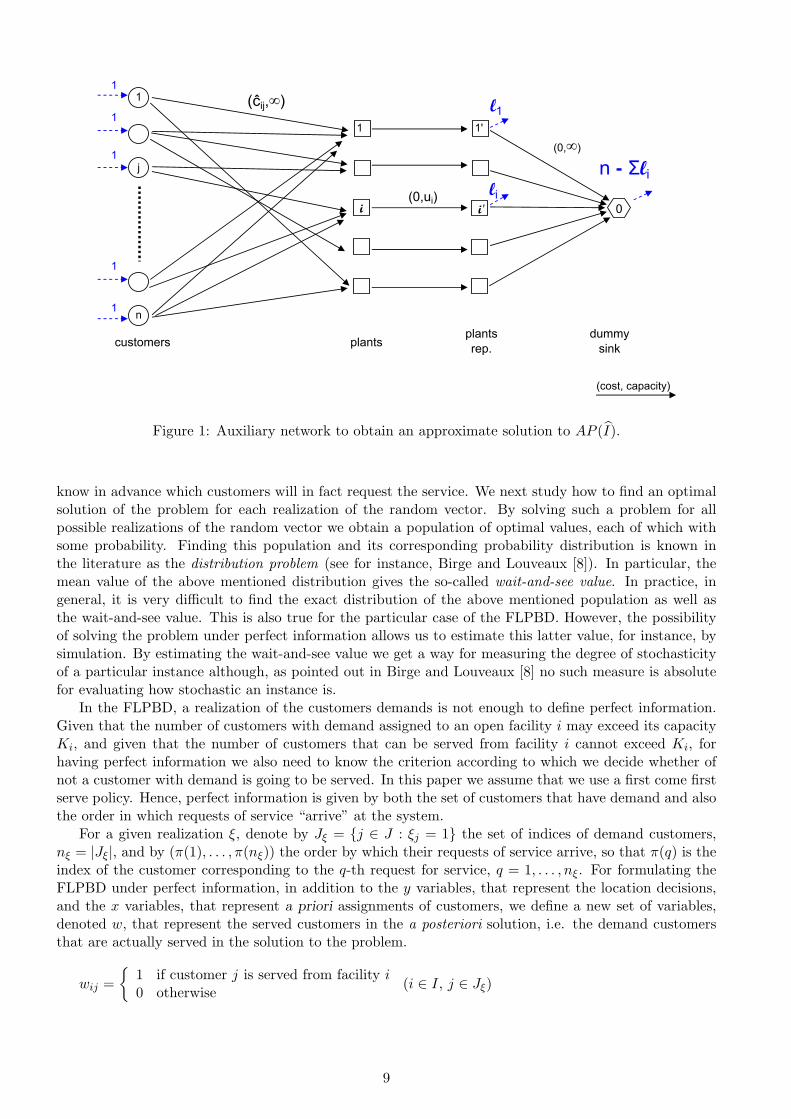
5.1 Constructive Phase

In the constructive phase we temporarily relax the constraints requiring each open plant to have aminimum number of assigned customers. Initially, one single facility is chosen to be opened and allcustomers are assigned to it. In a general step k a new plant is opened and some customers are reassignedto it, giving raise to a feasible solution (yk, xk). To choose the plant to open we estimate, for each closedplant, the incremental cost that would be incurred by opening it. The chosen plant is the one leadingto the lowest negative incremental cost, if any. The procedure stops when all incremental costs arenon-negative.

In each step k, denote by Ik the set of facilities that are open, and by i(j) the plant to which customer jis currently assigned (j ∈ J). Let also sk

i denote the number of customers assigned to a facility i ∈ Ik (i.e.ski = |{i : i(j) = i}|). Then, for each closed plant i ∈ I \ Ik, we compute the incremental cost for opening

it, say ∆ki , as the sum of the set-up cost of facility i plus an estimation of the variation in the assignment

costs when reassigning customers from its current assignment, taking into account the expected savingin the penalty for unserved customers. If one or several closed facilities have a negative incremental cost,we choose to open the one with the most negative incremental cost. The procedure continues until allthe closed facilities have a non-negative incremental cost. In the initialization step, for each plant i, the

maximum number of customers we allow to be assigned to facility i is ui = max

{Ki,

np

KiPt∈I

Kt

}following

the same rationale as in the definition of the network of Figure 1 in Section 3 (p denotes the average ofthe values pj , j ∈ J). We recall that zi denotes the number of customers assigned to facility i (i ∈ I).The procedure can be formalized as follows:'

&

$

%

Constructive phase for obtaining a feasible solution to FLPBD

1. Initialization:

• Compute the initial auxiliary capacities ui, i ∈ I, as follows

ui = min

{n, max

{Ki,

nKi

p∑

t∈I Kt

}}

• For i ∈ I let ∆0i = fi+ci

ui, where ci denotes the average assignment cost to facility

i.

• Let i0 ∈ I be such that ∆0i0 = mini∈I ∆0

i .

• I0 = {i0}; i(j) = i0, ∀j ∈ J ; zi0 = n, zi = 0, i ∈ I \ {i0}; k = 1.

2. While (k = 1 or ∆k−1ik−1 < 0) do

• For each i ∈ I, j ∈ J , compute the value δij = cij − ci(j)j − pj × g(zi(j)−Ki(j))

+

zi(j).

• Sort the customers by non-decreasing order of the values δij .Denote by j[q] (q = 1, . . . , n) the q-th customer after sorting.

• For i ∈ I, ∆ki = fi +

r∑t=1

δij[t] , with r = min{max{`i,max{q : δij[q]< 0}}, ui}

• Let ik ∈ I \ Ik−1 be such that ∆kik

= mini∈I\Ik−1 ∆ki .

• If ∆kik

< 0

Ik := Ik−1 ∪{ik}; zi(j) = zi(j)− 1, j = j[1], . . . , j[r]; i(j) = ik, j = j[1], . . . , j[r];

zik = zik + r; k := k + 1

As mentioned before, at termination of the constructive phase, we apply a second phase where an apriori assignment is obtained by solving the minimum cost flow problem of Section 3 as an approximationof the assignment problem AP (Ik).

11

5.2 Local Search

In the local search phase we consider two types of moves: reassignments and interchanges. In both caseswe estimate the variation in the total cost, instead of computing it exactly. The exact value of a solutionis computed after the constructive phase, and after the local search phase.

The two neighborhoods that we use in the local search are defined by reassignments of customerswithin the set of open plants, and by interchanges of assignments of pairs of customers, respectively.Below, we propose an estimate of the variation of the objective function value in each case:

ReassignmentsAn estimate for the variation in cost when reassigning customer j from plant i1 = i(j) to i2 is:

δj,i2 = ci2j − ci1j + g

(pj

zi2 + 1max{zi2 + 1−Ki2 , 0} −

pj

zi1

max{zi1 −Ki1 , 0})

In this expression, the termpj

zi2+1

max{zi2 + 1 − Ki2 , 0} is an estimate of the increase of the

expected penalty in plant i2, that will now have one more customer, whereas the termpj

zi1max{zi1−

Ki1 , 0} is an estimate of the reduction of the expected penalty in plant i1.

InterchangesWhen interchanging the assignment of two customers j1, j2, if we take i1 = i(j1), i2 = i(j2) and

we assume (without loss of generality) that pj1 > pj2 , the estimate for the cost variation is:

δj1j2 = ci1j2 + ci2j1 − ci1j1 − ci2j2 + (pj1 − pj2)g

(1

zi1

max{zi1 −Ki1 , 0} −1

zi2

max{zi2 −Ki2 , 0})

Note that for the situation in which pj = p ∀j, the penalty term is 0.

6 Computational Experiments

In this section we report the computational experience performed to evaluate the methodologiespresented above applied to the homogeneous case (pj = p, j ∈ J).

Due to the fact that no benchmark instances exist for the FLPBD, we considered two setsof instances existing in the literature for the capacitated single sourcing facility location problemnamely, those presented by Holmberg et al. [16] and Dıaz and Fernandez [14] (publicly availableat http://www-eio.upc.es/∼elena/sscplp/).

For each instance in each set, the demands of the customers were ignored, since now theyfollow a Bernoulli probability distribution, and new capacities Ki have been generated, coherentwith the Bernoulli demands, as follows. Each instance produced four instances for the FLPBDaccording to:

1. pj = 0.25 ∀j ∈ J , `i = 0 ∀i ∈ I, and Ki are generated as described below ∀i ∈ I.

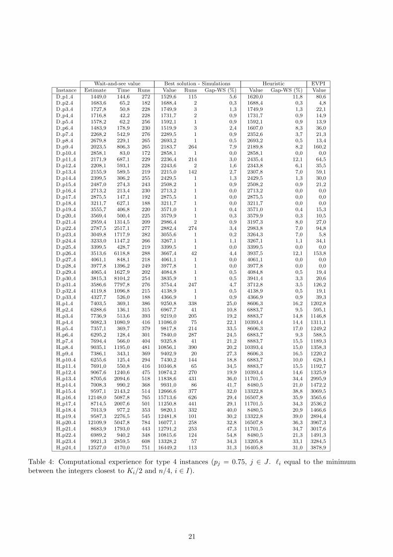
2. pj = 0.25 ∀j ∈ J . For each i ∈ I, Ki is generated as described below. Then, `i is set equalto the minimum between the nearest integers to Ki/2 and n/4.

3. pj = 0.75 ∀j ∈ J , `i = 0 ∀i ∈ I, and Ki are generated as described below ∀i ∈ I.

4. pj = 0.75 ∀j ∈ J . For each i ∈ I, Ki is generated as described below. Then, `i is set equalto the minimum between the nearest integers to Ki/2 and n/4.

For each instance, the capacities of the plants are generated as follows:

1. Generate a random number ρ in the set {1, 2, 3, 4, 5}, which represents a lower bound on thevalue that we accept for each Ki, i ∈ I.

12

2 For each plant i ∈ I

2.1 Define γi = fi

ci, where ci denotes the average assignment cost to facility i.

2.2 Define Γ =∑

i∈I γi.

2.3 Define λi = 32ϑi × n×p

Γ, where ϑi is a random number in [0.9γi; 1.1γi].

2.4 If λi < ρ set Ki = ρ; else, if λi > n set Ki = n; else, set Ki = λi.

In general terms, the capacities of the facilities are generated in such a way that the expectedoverall capacity is equal or close to 1.5np (recall that we are considering pj = p, j ∈ J). Notethat if Ki = λi ∀i ∈ I, then the expected overall capacity is exactly 1.5np, which is not the caseif some λi < ρ or λ > n. However, we expect the final value to be close to the target.

Note also that for each instance we first set the values pj (j ∈ J) and then we determine Ki

for all i ∈ I according to the steps above. Instances of types 1 and 2 share the same vector of Ki.The same happens with instances of types 3 and 4. This way, in both cases, for the same vectorof Ki two possible vectors of `i are considered.

Finally, for each instance, the penalty cost g was set equal to maxi∈I, j∈J

cij.

All the instances have a label with three components that allow an easy identification:

• A letter indicating the original set upon which the instance was built. ‘D’ denotes an instancefrom the set considered in Dıaz and Fernandez [14] and ‘H’ denotes one instance coming fromthe set presented in Holmberg et al. [16].

• The label of the original instance.

• The type of instance for FLPBD (1, 2, 3, or 4) as described above.

For example, ‘D p2 3’ refers to an instance of type 3 built from instance p2 taken from Dıazand Fernandez [14].

The computational results we present are based on instances p1-p33 from Dıaz and Fernandez [14]and instances p1-p24 from Holmberg et al. [16]. Taking into account the four types of instancesbuilt from each of these, in total we have 228 instances. The number of locations and the numberof customers for these instances are given in the following table:

Instance |I| |J |

Instances from Dıaz and Fernandez [14]

p1–p6 10 20p7–p17 15 30

p18–p25 20 40p26–p33 20 50

Instances from Holmberg et al. [16] p1–p12 10 50p13–p24 20 50

As it was mentioned in Section 4, in this paper we estimate the wait-and-see value by simula-tion. In particular, we consider the average of the optimal values of PI(ξ, π) solved for the differentrealizations randomly generated for the random vectors. These optimal values are obtained usingILOG CPLEX 11.0.

It is a well-known result from stochastic programming (see, for instance, Kall and Wallace [20])that in a minimization problem, the wait-and-see value can never be greater than the optimal valueof the stochastic problem. However, this is not necessarily true (and in general it is not) for allrealizations of the random vector. Accordingly, it may happen that the above mentioned average(that estimates the wait-and-see value) is greater than the value of some feasible solution found.When this is the case we take for the wait-and-see estimate the value of such feasible solution.

We defined as a stopping criterion for the simulation procedure an average variance below 10%of the average itself because this is a good indication that a very ‘stable’ value was achieved forthe average. However, to overcome situations in which the first iterations lead to very similarvalues, we set a minimum number of 30 simulations. On the other hand, to make sure that the

13

process would stop within a reasonable number of simulations we set a maximum number of 7500simulations.

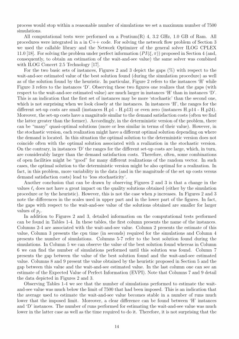
All computational tests were performed on a Pentium(R) 4, 3.2 GHz, 1.0 GB of Ram. Allprocedures were integrated in a in C++ code. For solving the network flow problem of Section 3we used the callable library and the Network Optimizer of the general solver ILOG CPLEX11.0 [18]. For solving the problem under perfect information (PI(ξ, π)) proposed in Section 4 (and,consequently, to obtain an estimation of the wait-and-see value) the same solver was combinedwith ILOG Concert 2.5 Technology [17].

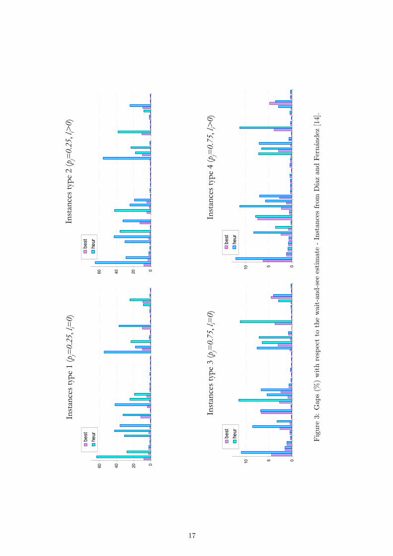
For the two basic sets of instances, Figures 2 and 3 depict the gaps (%) with respect to thewait-and-see estimated value of the best solution found (during the simulation procedure) as wellas of the solution found by the heuristic. In particular, Figure 2 refers to the instances ‘H’ whileFigure 3 refers to the instances ‘D’. Observing these two figures one realizes that the gaps (withrespect to the wait-and-see estimated value) are much larger in instances ‘H’ than in instances ‘D’.This is an indication that the first set of instances may be more ‘stochastic’ than the second one,which is not surprising when we look closely at the instances. In instances ‘H’, the ranges for thedifferent set-up costs are small (instances H p1 - H p13) or even zero (instances H p14 - H p24).Moreover, the set-up costs have a magnitude similar to the demand satisfaction costs (often we findthe latter greater than the former). Accordingly, in the deterministic version of the problem, therecan be “many” quasi-optimal solutions (more or less similar in terms of their value). However, inthe stochastic version, each realization might have a different optimal solution depending on wherethe demand is located. In this situation the optimal solution to the deterministic version does notcoincide often with the optimal solution associated with a realization in the stochastic version.On the contrary, in instances ‘D’ the ranges for the different set-up costs are large, which, in turn,are considerably larger than the demand satisfaction costs. Therefore, often, some combinationsof open facilities might be “good” for many different realizations of the random vector. In suchcases, the optimal solution to the deterministic version might be also optimal for a realization. Infact, in this problem, more variability in the data (and in the magnitude of the set up costs versusdemand satisfaction costs) lead to ‘less stochasticity’.

Another conclusion that can be drawn by observing Figures 2 and 3 is that a change in thevalues `i does not have a great impact on the quality solutions obtained (either by the simulationprocedure or by the heuristic). However, this is not the case when p increases. In Figures 2 and 3note the differences in the scales used in upper part and in the lower part of the figures. In fact,the gaps with respect to the wait-and-see value of the solutions obtained are smaller for largervalues of pj.

In addition to Figures 2 and 3, detailed information on the computational tests performedcan be found in Tables 1-4. In these tables, the first column presents the name of the instances.Columns 2-4 are associated with the wait-and-see value. Column 2 presents the estimate of thisvalue, Column 3 presents the cpu time (in seconds) required for the simulations and Column 4presents the number of simulations. Columns 5-7 refer to the best solution found during thesimulations. In Column 5 we can observe the value of the best solution found whereas in Column6 we can find the number of simulations performed until this solution was found. Column 7presents the gap between the value of the best solution found and the wait-and-see estimatedvalue. Columns 8 and 9 present the value obtained by the heuristic proposed in Section 5 and thegap between this value and the wait-and-see estimated value. In the last column one can see anestimate of the Expected Value of Perfect Information (EVPI). Note that Columns 7 and 9 detailthe data depicted in Figures 2 and 3.

Observing Tables 1-4 we see that the number of simulations performed to estimate the wait-and-see value was much below the limit of 7500 that had been imposed. This is an indication thatthe average used to estimate the wait-and-see value becomes stable in a number of runs muchlower that the imposed limit. Moreover, a clear difference can be found between ‘H’ instancesand ‘D’ instances. The number of runs performed for estimating the wait-and-see value was muchlower in the latter case as well as the time required to do it. Therefore, it is not surprising that the

14

same type of conclusions can be drawn for the number of runs performed before the best solutionwas found (Column 6). Note, also, that the number of runs required until the best solution wasfound is much lower than the total number of runs. This means that a very good solution isobtained early in the simulation procedure.

By observing the last column in Tables 1-4 (which gives an estimate of the EVPI) we confirmthe conclusion that was drawn above about the difference in the ‘degree of stochasticity’ betweeninstances ‘H’ and ‘D’. In fact, the EVPI is a measure (even if not always very robust) of the‘degree of stochasticity’ of an instance (see, for instance, Birge and Louveaux [8]). As we can see,the EVPI is quite small in instances ‘D’ and often is equal to 0.

It is very important to observe the performance of the heuristic in the two sets of instances. Incomparison with the best solution found during the simulation procedure, the heuristic performsmuch better in instances ‘H’ than in instances ‘D’. This is very important because it gives evidencethat the heuristic performs better in instances with a greater ‘degree of stochasticity’, which isa very important feature. In fact, the heuristic was designed for the stochastic case and a goodbehavior in instances with ‘more stochasticity’ is highly desirable. It should be pointed out thatthe cpu time required by the heuristic was always below 1 second (and this is the reason why thethis cpu time is not presented in Tables 1-4).

As mentioned before, the possibility of working with the FLPBD in the non-homogeneoussituation, relies on the approximation of the objective function stated in Proposition 2. Only forinstances with a very small |J | would we be able to evaluate the quality of the approximation.Accordingly, no results are presented for this situation because for instances with a size similarto the ones presented in Tables 1-4, it is already unaffordable to compute exactly the recoursefunction, which means that the quality of the approximation could not be measured. Therefore,any computational experience we presented for such case would be meaningless in the sense thatthe quality of the results could only be measured for instances where the conditions for theapproximation do not hold.

7 Conclusions and directions for further research

In this paper we studied a facility location problem with Bernoulli demands. We proposed atwo-stage stochastic programming model for the problem. We showed that the recourse functionhas a closed form. For the non-homogeneous case the exact evaluation of the recourse functionbecomes unaffordable when a large number of customers is assigned a priori to the operatingfacilities. In this case we used the central limit theorem to show that the recourse function canbe approximated. We studied the stochastic assignment problem arising when a decision hasbeen made on the operating facilities. Again, we propose approximating the optimal solution tothis problem, which can be accomplished by solving a minimum cost network flow problem onan auxiliary network. We study the problem under perfect information. Finally, we propose aheuristic for finding an a priori solution to the problem. We present results from computationalexperience for the homogeneous case. The results indicate that it is possible to estimate the wait-and-see value as well as the expected value of perfect information with an affordable computationaleffort. Moreover, a good a priori solution can be found by using the simulation procedure thatestimates the wait-and-see value. For instances with a large degree of ‘stochasticity’ the heuristicproposed can obtain even better results with a very small computational effort.

In the future, it would be interesting to study the possibility of extending the results andmethodologies presented in this paper to more general situations namely, by considering otherprobability distributions for the demands and a multi-period setting for locating the facilities.Another opened direction for further research regards the algorithmic use of the normal approxi-mation of the recourse function for the non-homogeneous case.

15

0

20

40

60

80

100

120

140

best

heur.

0

20

40

60

80

100

120

140

best

heur.

0

20

40

best

heur.

0

20

40

best

heur.

Instances type 1 (p j=0.25, l i=0)

Instances type 2 (p j=0.25, l i>0)

Instances type 3 (p j=0.75, l i=0)

Instances type 4 (p j=0.75, l i>0)

Fig

ure

2:G

aps

(%)

wit

hre

spec

tto

the

wai

t-an

d-se

ees

tim

ate

-In

stan

ces

from

Hol

mbe

rget

al.[1

6].

16

05

10

best

heur

0

20

40

60

best

heur

0

20

40

60

best

heur

05

10

best

heur

Instances type 1 (p j=0.25, l i=0)

Instances type 2 (p j=0.25, l i>0)

Instances type 3 (p j=0.75, l i=0)

Instances type 4 (p j=0.75, l i>0)

Fig

ure

3:G

aps

(%)

wit

hre

spec

tto

the

wai

t-an

d-se

ees

tim

ate

-In

stan

ces

from

Dıa

zan

dFe

rnan

dez

[14]

.

17

Wait-and-see value Best solution - Simulations Heuristic EVPIInstance Estimate Time Runs Value Runs Gap-WS (%) Value Gap-WS (%) ValueD p1 1 509,7 43,8 629 549,2 4 7,8 833,2 63,5 39,5D p2 1 682,5 36,1 566 699,3 1 2,5 873,8 28,0 16,8D p3 1 734,8 25,7 441 761,1 1 3,6 761,1 3,6 26,4D p4 1 743,0 24,3 547 743,0 1 0,0 743,0 0,0 0,0D p5 1 593,0 22,4 561 603,5 1 1,8 779,1 31,4 10,5D p6 1 504,8 61,9 700 531,2 3 5,3 739,6 46,5 26,5D p7 1 801,3 115,8 725 804,6 2 0,4 1084,1 35,3 3,3D p8 1 1208,0 46,5 475 1208,4 1 0,0 1208,4 0,0 0,4D p9 1 665,5 135,4 677 739,0 22 11,0 874,2 31,4 73,5D p10 1 1365,4 22,3 370 1373,2 1 0,6 1373,2 0,6 7,8D p11 1 738,0 188,1 744 765,8 1 3,8 1045,8 41,7 27,8D p12 1 750,1 144,9 740 758,7 1 1,2 929,4 23,9 8,7D p13 1 713,0 157,5 763 740,7 4 3,9 840,4 17,9 27,8D p14 1 937,4 70,8 615 944,6 1 0,8 944,6 0,8 7,2D p15 1 1003,5 66,7 530 1023,4 1 2,0 1023,4 2,0 19,9D p16 1 1214,5 45,8 454 1228,4 1 1,1 1228,4 1,1 13,9D p17 1 1378,3 35,0 388 1390,6 1 0,9 1390,6 0,9 12,3D p18 1 1231,7 148,0 616 1231,7 1 0,0 1231,7 0,0 0,0D p19 1 1591,0 99,8 499 1591,0 1 0,0 1591,0 0,0 0,0D p20 1 1599,9 113,4 497 1599,9 1 0,0 1599,9 0,0 0,0D p21 1 1006,4 353,2 810 1006,4 1 0,0 1552,9 54,3 0,0D p22 1 866,2 374,7 780 954,6 389 10,2 1026,1 18,5 88,4D p23 1 1075,1 307,1 690 1075,6 1 0,1 1318,9 22,7 0,6D p24 1 1273,1 169,6 570 1287,1 2 1,1 1287,1 1,1 13,9D p25 1 1419,5 105,4 516 1419,5 1 0,0 1419,5 0,0 0,0D p26 1 1130,3 654,6 686 1238,2 279 9,6 1550,4 37,2 108,0D p27 1 1574,7 213,4 625 1586,1 1 0,7 1586,1 0,7 11,4D p28 1 1498,2 229,5 661 1502,8 1 0,3 1502,8 0,3 4,6D p29 1 1595,3 233,4 518 1609,8 1 0,9 1609,8 0,9 14,5D p30 1 1356,1 562,7 655 1360,9 2 0,4 1467,9 8,3 4,9D p31 1 1115,9 624,8 768 1233,7 61 10,6 1408,0 26,2 117,8D p32 1 1649,1 205,0 559 1663,9 1 0,9 1663,9 0,9 14,8D p33 1 1870,2 174,6 494 1891,9 1 1,2 1891,9 1,2 21,7H p1 1 3906,6 632,5 2292 7293,2 781 86,7 6496,7 66,3 2590,1H p2 1 3305,2 328,4 1838 6624,7 1825 100,4 5342,5 61,6 2037,4H p3 1 4526,0 986,3 2672 7995,8 1072 76,7 7342,5 62,2 2816,6H p4 1 5686,4 1992,3 3364 8963,6 1700 57,6 9342,5 64,3 3277,2H p5 1 3926,0 628,8 2314 7332,2 1911 86,8 6496,7 65,5 2570,7H p6 1 3335,1 381,0 2093 6776,5 1490 103,2 5342,5 60,2 2007,5H p7 1 4540,0 932,7 2485 8144,7 1243 79,4 7342,5 61,7 2802,5H p8 1 5724,8 1933,0 3343 8992,5 877 57,1 9342,5 63,2 3267,8H p9 1 3925,1 626,9 2289 7396,0 1532 88,4 6496,7 65,5 2571,6H p10 1 3316,1 347,1 1905 6837,2 114 106,2 5342,5 61,1 2026,4H p11 1 4550,4 973,7 2567 8106,4 1571 78,2 7342,5 61,4 2792,1H p12 1 5723,5 1874,1 3275 8932,8 1202 56,1 9342,5 63,2 3209,3H p13 1 3833,7 1344,5 2061 7937,3 536 107,0 8231,5 114,7 4103,6H p14 1 3118,6 653,9 1531 7738,7 979 148,2 6888,9 120,9 3770,3H p15 1 4407,9 2233,0 2201 8986,8 272 103,9 9431,1 114,0 4578,9H p16 1 5726,7 6360,1 2927 9851,2 1173 72,0 11470,1 100,3 4124,5H p17 1 3864,5 1375,1 1996 7967,3 603 106,2 8231,5 113,0 4102,8H p18 1 3117,2 593,9 1478 7572,7 1416 142,9 6888,9 121,0 3771,7H p19 1 4450,3 2261,6 2092 8738,9 702 96,4 9431,1 111,9 4288,6H p20 1 5730,7 6412,1 2960 9807,5 658 71,1 11470,1 100,2 4076,8H p21 1 3852,2 1379,1 2063 7846,6 1805 103,7 8231,5 113,7 3994,4H p22 1 3107,5 553,4 1405 7715,7 12 148,3 6888,9 121,7 3781,4H p23 1 4448,5 2299,2 2164 8882,9 654 99,7 9431,1 112,0 4434,5H p24 1 5715,7 6130,9 2920 9823,5 1888 71,9 11470,1 100,7 4107,8

Table 1: Computational experience for type 1 instances (pj = 0.25, j ∈ J and `i = 0, i ∈ I).

18

Wait-and-see value Best solution - Simulations Heuristic EVPIInstance Estimate Time Runs Value Runs Gap-WS (%) Value Gap-WS (%) ValueD p1 2 497,0 48,6 700 549,2 4 10,5 839,0 68,8 52,2D p2 2 668,5 27,1 483 699,3 3 4,6 873,8 30,7 30,9D p3 2 732,3 22,5 457 761,1 6 3,9 761,1 3,9 28,8D p4 2 721,2 22,5 501 743,0 1 3,0 743,0 3,0 21,7D p5 2 595,2 25,6 643 603,5 1 1,4 779,1 30,9 8,3D p6 2 520,4 56,6 687 531,2 1 2,1 739,6 42,1 10,9D p7 2 794,5 107,8 625 804,6 1 1,3 1084,1 36,4 10,1D p8 2 1206,6 48,5 456 1208,4 1 0,1 1208,4 0,1 1,7D p9 2 669,3 131,4 611 739,0 154 10,4 871,3 30,2 69,7D p10 2 1373,2 28,0 426 1373,2 1 0,0 1373,2 0,0 0,0D p11 2 729,1 202,0 709 765,8 12 5,0 1045,8 43,4 36,6D p12 2 746,9 164,1 746 758,7 2 1,6 929,4 24,4 11,8D p13 2 702,9 173,8 760 740,7 2 5,4 840,4 19,6 37,8D p14 2 940,1 71,0 582 944,6 1 0,5 944,6 0,5 4,5D p15 2 1023,4 72,4 539 1023,4 1 0,0 1023,4 0,0 0,0D p16 2 1228,4 46,5 430 1228,4 1 0,0 1228,4 0,0 0,0D p17 2 1388,3 36,5 395 1390,6 1 0,2 1390,6 0,2 2,3D p18 2 1219,6 148,4 604 1231,7 1 1,0 1231,7 1,0 12,1D p19 2 1574,3 90,7 452 1591,0 1 1,1 1591,0 1,1 16,7D p20 2 1599,9 108,9 453 1599,9 1 0,0 1599,9 0,0 0,0D p21 2 1006,4 360,5 753 1006,4 1 0,0 1552,9 54,3 0,0D p22 2 867,2 380,3 759 962,3 690 11,0 1025,7 18,3 95,1D p23 2 1075,6 349,6 717 1075,6 1 0,0 1318,9 22,6 0,0D p24 2 1272,7 186,2 586 1287,1 2 1,1 1287,1 1,1 14,3D p25 2 1419,5 116,6 530 1419,5 1 0,0 1419,5 0,0 0,0D p26 2 1103,0 694,8 705 1238,2 656 12,3 1550,4 40,6 135,3D p27 2 1580,7 236,3 640 1586,1 1 0,3 1586,1 0,3 5,4D p28 2 1492,6 222,8 602 1502,8 1 0,7 1502,8 0,7 10,2D p29 2 1575,9 246,0 532 1609,8 1 2,2 1609,8 2,1 33,9D p30 2 1360,9 689,3 752 1360,9 1 0,0 1467,9 7,9 0,0D p31 2 1146,4 785,8 742 1256,8 645 9,6 1408,0 22,8 110,4D p32 2 1663,9 212,2 557 1663,9 1 0,0 1663,9 0,0 0,0D p33 2 1887,2 176,1 452 1891,9 1 0,3 1891,9 0,2 4,7H p1 2 3890,6 576,2 2174 7541,5 2014 93,8 6496,7 67,0 2606,2H p2 2 3332,8 354,6 1963 6689,2 1099 100,7 5342,5 60,3 2009,8H p3 2 4525,1 894,6 2614 8130,4 201 79,7 7342,5 62,3 2817,4H p4 2 5736,9 1983,1 3434 9015,0 2804 57,1 9342,5 62,8 3278,1H p5 2 3901,9 618,3 2271 7431,3 1925 90,5 6496,7 66,5 2594,8H p6 2 3319,7 350,6 1954 6794,2 313 104,7 5342,5 60,9 2022,8H p7 2 4545,1 881,1 2460 7996,9 921 75,9 7342,5 61,5 2797,4H p8 2 5738,4 1881,3 3333 8981,4 1007 56,5 9342,5 62,8 3243,0H p9 2 3889,4 650,3 2456 7282,1 676 87,2 6496,7 67,0 2607,3H p10 2 3341,3 360,3 1994 6778,6 335 102,9 5342,5 59,9 2001,2H p11 2 4522,2 850,3 2463 8089,4 2397 78,9 7342,5 62,4 2820,4H p12 2 5724,2 1824,6 3276 8999,9 864 57,2 9342,5 63,2 3275,7H p13 2 3848,1 1539,1 1951 7865,9 1560 104,4 8231,5 113,9 4017,8H p14 2 3116,3 703,1 1559 7500,5 1054 140,7 6888,9 121,1 3772,6H p15 2 4472,5 2929,9 2163 8744,3 115 95,5 9431,1 110,9 4271,8H p16 2 5745,6 10167,7 2892 9962,5 416 73,4 11470,1 99,6 4216,9H p17 2 3849,2 1531,9 1996 7925,9 1338 105,9 8231,5 113,8 4076,7H p18 2 3138,6 704,3 1510 7355,9 166 134,4 6888,9 119,5 3750,2H p19 2 4430,5 2877,1 2198 8897,7 1673 100,8 9431,1 112,9 4467,2H p20 2 5730,0 10947,1 3042 9918,3 2795 73,1 11470,1 100,2 4188,3H p21 2 3891,9 1615,8 2066 8150,7 1971 109,4 8231,5 111,5 4258,8H p22 2 3123,6 696,6 1491 7423,1 352 137,7 6888,9 120,5 3765,3H p23 2 4449,8 2910,1 2222 8966,5 698 101,5 9431,1 111,9 4516,7H p24 2 5726,5 9131,1 2831 9938,0 705 73,5 11470,1 100,3 4211,4

Table 2: Computational experience for type 2 instances (pj = 0.25, j ∈ J . `i equal to the minimumbetween the integers closest to Ki/2 and n/4, (i ∈ I) ).

19

Wait-and-see value Best solution - Simulations Heuristic EVPIInstance Estimate Time Runs Value Runs Gap-WS (%) Value Gap-WS (%) ValueD p1 3 1481,7 196,4 234 1525,6 18 3,0 1620,0 9,3 44,0D p2 3 1651,7 140,7 244 1688,4 1 2,2 1688,4 2,2 36,7D p3 3 1730,8 82,2 233 1749,9 1 1,1 1749,9 1,1 19,1D p4 3 1721,0 42,3 237 1731,7 1 0,6 1731,7 0,6 10,7D p5 3 1589,5 60,8 246 1592,1 1 0,2 1592,1 0,2 2,6D p6 3 1473,2 297,6 275 1519,9 5 3,2 1607,0 9,1 46,7D p7 3 2268,0 571,7 318 2289,5 1 1,0 2352,6 3,7 21,5D p8 3 2693,2 162,6 178 2693,2 1 0,0 2693,2 0,0 0,0D p9 3 2064,5 612,1 227 2195,7 91 6,4 2189,8 6,1 125,3D p10 3 2858,1 94,3 202 2858,1 1 0,0 2858,1 0,0 0,0D p11 3 2184,9 864,3 290 2242,9 84 2,7 2435,4 11,5 58,0D p12 3 2222,6 636,8 264 2243,6 2 1,0 2343,8 5,5 21,0D p13 3 2154,7 689,8 255 2217,6 197 2,9 2307,8 7,1 62,9D p14 3 2419,1 243,0 209 2429,5 1 0,4 2429,5 0,4 10,4D p15 3 2508,2 228,0 206 2508,2 1 0,0 2508,2 0,0 0,0D p16 3 2713,2 164,8 193 2713,2 1 0,0 2713,2 0,0 0,0D p17 3 2865,4 142,8 204 2875,5 2 0,4 2875,5 0,4 10,1D p18 3 3210,5 706,5 208 3211,7 1 0,0 3211,7 0,0 1,2D p19 3 3571,0 353,8 194 3571,0 1 0,0 3571,0 0,0 0,0D p20 3 3565,8 449,8 195 3579,9 1 0,4 3579,9 0,4 14,1D p21 3 2964,9 1231,7 220 2986,4 1 0,7 3200,4 7,9 21,5D p22 3 2822,3 2168,7 252 2886,4 57 2,3 2983,8 5,7 64,1D p23 3 3046,1 1193,1 215 3055,6 1 0,3 3264,3 7,2 9,5D p24 3 3256,1 1013,3 226 3267,1 2 0,3 3267,1 0,3 10,9D p25 3 3399,5 422,6 230 3399,5 1 0,0 3399,5 0,0 0,0D p26 3 3529,1 5948,0 322 3655,0 304 3,6 3937,5 11,6 125,9D p27 3 4049,9 817,1 220 4061,1 1 0,3 4061,1 0,3 11,2D p28 3 3977,8 1076,6 223 3977,8 1 0,0 3977,8 0,0 0,0D p29 3 4084,8 1407,7 206 4084,8 2 0,0 4084,8 0,0 0,0D p30 3 3815,3 8194,3 300 3835,9 1 0,5 3941,4 3,3 20,6D p31 3 3587,3 5415,8 253 3721,6 149 3,7 3712,8 3,5 125,5D p32 3 4134,8 1055,0 226 4138,9 1 0,1 4138,9 0,1 4,1D p33 3 4343,5 622,6 211 4366,9 1 0,5 4366,9 0,5 23,5H p1 3 7401,5 315,7 350 9836,0 114 32,9 8648,4 16,8 1246,9H p2 3 6344,2 122,3 294 7605,4 264 19,9 6883,7 8,5 539,5H p3 3 7707,0 490,2 389 9406,6 216 22,1 8883,7 15,3 1176,7H p4 3 8998,6 1000,1 421 11901,6 145 32,3 10393,4 15,5 1394,8H p5 3 7433,1 366,6 414 9139,6 62 23,0 8648,4 16,4 1215,3H p6 3 6301,7 125,5 309 7530,0 128 19,5 6883,7 9,2 582,0H p7 3 7701,0 482,6 345 10000,8 113 29,9 8883,7 15,4 1182,7H p8 3 9073,5 1249,8 489 11712,3 80 29,1 10393,4 14,5 1319,9H p9 3 7369,2 358,7 403 10057,0 268 36,5 8648,4 17,4 1279,2H p10 3 6315,5 121,6 299 8094,7 212 28,2 6883,7 9,0 568,2H p11 3 7751,6 499,9 369 9490,1 318 22,4 8883,7 14,6 1132,1H p12 3 9055,7 993,9 386 11829,2 131 30,6 10393,4 14,8 1337,8H p13 3 8678,0 1617,8 439 12543,1 310 44,5 11742,7 35,3 3064,8H p14 3 7022,0 1105,1 412 9579,9 353 36,4 8677,5 23,6 1655,5H p15 3 9529,2 2429,5 626 13410,4 338 40,7 13332,5 39,9 3803,4H p16 3 12156,6 5434,9 810 16119,8 137 32,6 16517,5 35,9 3963,2H p17 3 8636,5 1897,5 523 11816,4 359 36,8 11742,7 36,0 3106,2H p18 3 7023,6 872,8 333 10638,6 331 51,5 8677,5 23,5 1653,9H p19 3 9578,5 2244,0 558 12628,4 141 31,8 13332,5 39,2 3049,9H p20 3 12076,5 4967,6 741 16456,1 85 36,3 16517,5 36,8 4379,6H p21 3 8687,2 2148,6 575 12115,6 136 39,5 11742,7 35,2 3055,5H p22 3 6976,8 995,6 387 9849,3 196 41,2 8677,5 24,4 1700,8H p23 3 9937,0 2575,8 568 13149,7 120 32,3 13204,4 32,9 3212,7H p24 3 12489,3 3828,8 760 16158,6 327 29,4 16404,4 31,3 3669,4

Table 3: Computational experience for type 3 instances (pj = 0.75, j ∈ J and `i = 0, i ∈ I).

20

Wait-and-see value Best solution - Simulations Heuristic EVPIInstance Estimate Time Runs Value Runs Gap-WS (%) Value Gap-WS (%) ValueD p1 4 1449,0 144,6 272 1529,6 115 5,6 1620,0 11,8 80,6D p2 4 1683,6 65,2 182 1688,4 2 0,3 1688,4 0,3 4,8D p3 4 1727,8 50,8 228 1749,9 3 1,3 1749,9 1,3 22,1D p4 4 1716,8 42,2 228 1731,7 2 0,9 1731,7 0,9 14,9D p5 4 1578,2 62,2 256 1592,1 1 0,9 1592,1 0,9 13,9D p6 4 1483,9 178,9 230 1519,9 3 2,4 1607,0 8,3 36,0D p7 4 2268,2 542,9 276 2289,5 1 0,9 2352,6 3,7 21,3D p8 4 2679,8 229,1 265 2693,2 1 0,5 2693,2 0,5 13,4D p9 4 2023,5 806,3 265 2183,7 264 7,9 2189,8 8,2 160,2D p10 4 2858,1 83,0 172 2858,1 1 0,0 2858,1 0,0 0,0D p11 4 2171,9 687,1 229 2236,4 214 3,0 2435,4 12,1 64,5D p12 4 2208,1 593,1 228 2243,6 2 1,6 2343,8 6,1 35,5D p13 4 2155,9 589,5 219 2215,0 142 2,7 2307,8 7,0 59,1D p14 4 2399,5 306,2 255 2429,5 1 1,3 2429,5 1,3 30,0D p15 4 2487,0 274,3 243 2508,2 1 0,9 2508,2 0,9 21,2D p16 4 2713,2 213,4 230 2713,2 1 0,0 2713,2 0,0 0,0D p17 4 2875,5 147,1 192 2875,5 1 0,0 2875,5 0,0 0,0D p18 4 3211,7 627,1 188 3211,7 1 0,0 3211,7 0,0 0,0D p19 4 3555,7 406,8 220 3571,0 1 0,4 3571,0 0,4 15,3D p20 4 3569,4 500,4 225 3579,9 1 0,3 3579,9 0,3 10,5D p21 4 2959,4 1314,5 209 2986,4 2 0,9 3197,3 8,0 27,0D p22 4 2787,5 2517,1 277 2882,4 274 3,4 2983,8 7,0 94,8D p23 4 3049,8 1717,9 282 3055,6 1 0,2 3264,3 7,0 5,8D p24 4 3233,0 1147,2 266 3267,1 1 1,1 3267,1 1,1 34,1D p25 4 3399,5 428,7 219 3399,5 1 0,0 3399,5 0,0 0,0D p26 4 3513,6 6118,8 288 3667,4 42 4,4 3937,5 12,1 153,8D p27 4 4061,1 848,1 218 4061,1 1 0,0 4061,1 0,0 0,0D p28 4 3977,8 1396,2 249 3977,8 1 0,0 3977,8 0,0 0,0D p29 4 4065,4 1627,9 202 4084,8 1 0,5 4084,8 0,5 19,4D p30 4 3815,3 8104,2 254 3835,9 1 0,5 3941,4 3,3 20,6D p31 4 3586,6 7797,8 276 3754,4 247 4,7 3712,8 3,5 126,2D p32 4 4119,8 1096,8 215 4138,9 1 0,5 4138,9 0,5 19,1D p33 4 4327,7 526,0 188 4366,9 1 0,9 4366,9 0,9 39,3H p1 4 7403,5 369,1 386 9250,8 338 25,0 8606,3 16,2 1202,8H p2 4 6288,6 136,1 315 6967,7 41 10,8 6883,7 9,5 595,1H p3 4 7736,9 513,6 393 9219,0 205 19,2 8883,7 14,8 1146,8H p4 4 9082,3 1080,9 416 11086,0 75 22,1 10393,4 14,4 1311,1H p5 4 7357,1 369,7 379 9817,8 214 33,5 8606,3 17,0 1249,2H p6 4 6295,2 128,4 301 7840,0 287 24,5 6883,7 9,3 588,5H p7 4 7694,4 566,0 404 9325,8 41 21,2 8883,7 15,5 1189,3H p8 4 9035,1 1195,0 481 10856,1 390 20,2 10393,4 15,0 1358,3H p9 4 7386,1 343,1 369 9402,9 20 27,3 8606,3 16,5 1220,2H p10 4 6255,6 125,4 294 7430,2 144 18,8 6883,7 10,0 628,1H p11 4 7691,0 550,8 416 10346,8 65 34,5 8883,7 15,5 1192,7H p12 4 9067,6 1240,6 475 10874,2 270 19,9 10393,4 14,6 1325,9H p13 4 8705,6 2094,6 518 11838,6 431 36,0 11701,5 34,4 2995,9H p14 4 7008,3 990,2 368 9931,0 86 41,7 8480,5 21,0 1472,2H p15 4 9597,1 2143,2 514 12666,6 377 32,0 13322,8 38,8 3069,5H p16 4 12148,0 5087,8 765 15713,6 626 29,4 16507,8 35,9 3565,6H p17 4 8714,5 2007,6 501 11250,8 441 29,1 11701,5 34,3 2536,2H p18 4 7013,9 977,2 353 9820,1 332 40,0 8480,5 20,9 1466,6H p19 4 9587,3 2276,5 545 12481,8 101 30,2 13322,8 39,0 2894,4H p20 4 12109,9 5047,8 784 16077,1 258 32,8 16507,8 36,3 3967,3H p21 4 8683,9 1793,0 443 12791,2 253 47,3 11701,5 34,7 3017,6H p22 4 6989,2 940,2 348 10815,6 124 54,8 8480,5 21,3 1491,3H p23 4 9921,3 2859,5 608 13328,2 57 34,3 13205,8 33,1 3284,5H p24 4 12527,0 4170,0 751 16449,2 113 31,3 16405,8 31,0 3878,9

Table 4: Computational experience for type 4 instances (pj = 0.75, j ∈ J . `i equal to the minimumbetween the integers closest to Ki/2 and n/4, i ∈ I).

21

Acknowledgement

This research has been partially supported by the Spanish Ministry of Science and Education,Project MTM 2006-14961-C05-01, and by the Portuguese Science Foundation, Project POCTI -ISFL - 1 - 152.

References

[1] M. Albareda-Sambola, E. Fernandez, and G. Laporte. Heuristic and lower bounds for astochastic location routing problem. European Journal of Operational Research, 179:940–955,2007.

[2] M. Albareda-Sambola, M.H. van der Vlerk, and E. Fernandez. Exact solutions to a classof stochastic generalized assignment problems. European Journal of Operational Research,173:465–487, 2006.

[3] I. Averbakh and O. Berman. Minimax regret p-center location on a network with demanduncertainty. Location Science, 5:247–254, 1997.

[4] I. Averbakh and O. Berman. Minmax regret median location on a network under uncertainty.INFORMS Journal on Computing, 12:104–110, 2000.

[5] I. Averbakh and O. Berman. An improved algorithm for the minmax regret median problemon a tree. Networks, 41:97–103, 2003.

[6] O. Berman and D. Simchi-Levi. Finding the optimal a priori tour and location of a travelingsalesman with non homogeneous customers. Transportation Science, 22:148–154, 1988.

[7] L. Bianchi and A. M. Campbell. Extension of the 2-p-opt and 1-shift algorithms to theheterogeneous probabilistic traveling salesman problem. European Journal of OperationalResearch, 176:131–144, 2007.

[8] J.F. Birge and F. Louveaux. Introduction to Stochastic Programming. Springer Series inOperations Research. Springer, New York, 1997.

[9] M.L. Brandeau and S.S. Chiu. An overview of representative problems in location research.Management Science, 35:645–674, 1989.

[10] E. Carrizosa, E. Conde, and M. Munoz. Admission policies in loss queueing models withheterogeneus arrivals. Management Science, 44:311–320, 1998.

[11] E. Carrizosa and S. Nickel. Robust facility location. Mathematical Methods in OperationsResearch, 58:331–349, 2003.

[12] E. Conde. A branch and bound algorithm for the minimax regret spanning arborescence.Journal of Global Optimization, 37:467–480, 2007.

[13] E. Conde. Minmax regret location-allocation problem on a network under uncertainty. Eu-ropean Journal of Operational Research, 179:1025–1039, 2007.

[14] J.A. Dıaz and E. Fernandez. A branch-and-price algorithm for the single source capacitatedplant location problem. Journal of the Operational Research Society, 53:728–740, 2002.

[15] E. Fernandez, Y. Hinojosa, and J. Puerto. Filtering policies in loss queuing-location problems.Annals of Operations Research, 136:259–283, 2005.

22

[16] K. Holmberg, M. Ronnqvist, and D. Yuan. An exact algorithm for the capacitated facilitylocation problem with single sourcing. European Journal of Operational Research, 113:544–559, 1999.

[17] ILOG Concert Technology 2.5 User’s Manual. ILOG, Inc., Incline Village, Nevada, 2007.http://www.ilog.com/products/optimization/tech/concert.cfm.

[18] ILOG CPLEX 11.0 User’s Manual. ILOG, Inc., Incline Village, Nevada, 2007.http://www.ilog.fr/products/cplex/.

[19] P. Jaillet. A priori solution of a traveling salesman problem in which a random subset of thecustomers are visited. Operations Research, 36:929–936, 1988.

[20] P. Kall and S. Wallace. Stochastic Programming. John Wiley & Sons, New York, 1994.

[21] G. Laporte, F.V. Louveaux, and H. Mercure. An exact solution for the a priori optimizationof the probabilistic traveling salesman problem. Operations Research, 42:543–549, 1994.

[22] G. Laporte, F.V. Louveaux, and L. Van Hamme. Exact solution to a location problem withstochastic demands. Transportation Science, 28:95–103, 1994.

[23] F. Louveaux. Stochastic location analysis. Location Science, 1:127–154, 1993.

[24] F.V. Louveaux and D. Peeters. A dual-based procedure for stochastic facility location. Op-erations Research, 40:564–573, 1992.

[25] V. Marianov and C. ReVelle. The queueing maximal availability location problem: a modelfor the siting of emergency vehicles. European Journal of Operational Research, 93:110–120,1996.

[26] C. ReVelle. Review, extension and prediction in emergency service siting. European Journalof Operational Research, 40:58–69, 1989.

[27] M. Riis and K.A. Andersen. Capacitated network design with uncertain demand. INFORMSJournal on Computing, pages 247–260, 2002.

[28] L.V. Snyder. Facility location under uncertainty: A review. IIE Transactions, 38:537–554,2006.

[29] C. Toregas, R. Swain, and C. ReVelle. The location of emergency service facilities. OperationsResearch, 19:1363–1373, 1971.

23