The Evolution of Morals under Indirect Reciprocity
46
ISSN: 1439-2305 Number 370 – May 2019 THE EVOLUTION OF MORALS UNDER INDIRECT RECIPROCITY Revised Version June 2019 Alexia Gaudeul Claudia Keser Stephan Müller
Transcript of The Evolution of Morals under Indirect Reciprocity

ISSN: 1439-2305
Number 370 – May 2019
THE EVOLUTION OF MORALS UNDER
INDIRECT RECIPROCITY
Revised Version June 2019
Alexia Gaudeul
Claudia Keser
Stephan Müller

The Evolution of Morals under Indirect Reciprocity
Alexia Gaudeul∗1, Claudia Keser†1, and Stephan Muller‡1
1University of Gottingen
June 2019
Abstract
We study the coexistence of strategies in the indirect reciprocity game where agents
have access to second-order information. We fully characterize the evolutionary sta-
ble equilibria and analyze their comparative statics with respect to the cost-benefit
ratio (CBR). There are indeed only two stable sets of equilibria enabling coopera-
tion, one for low CBRs involving two strategies and one for higher CBR’s which in-
volves two additional strategies. We thereby offer an explanation for the coexistence
of different moral judgments among humans. Both equilibria require the presence of
second-order discriminators which highlights the necessity for higher-order informa-
tion to sustain cooperation through indirect reciprocity. In a laboratory experiment,
we find that more than 75% of subjects play strategies that belong to the predicted
equilibrium set. Furthermore, varying the CBR across treatments leads to changes
in the distribution of strategies that are in line with theoretical predictions.
JEL Classification numbers: C73, C91, D83
Keywords: Indirect reciprocity, Cooperation, Evolution, Experiment
∗Platz der Gottinger Sieben 5, 37073 Gottingen (Germany), E-mail: [email protected]
goettingen.de
†Platz der Gottinger Sieben 3, 37073 Gottingen (Germany), E-mail: [email protected]
‡Corresponding author, Platz der Gottinger Sieben 3, 37073 Gottingen (Germany), E-mail:

1 Introduction
Several theories have been proposed to explain the evolution of cooperation among hu-
mans when cooperation generates a public benefit at a private cost. One of the different
mechanisms to promote cooperation proposed in the literature is indirect reciprocity.1
Contrary to direct reciprocity, under indirect reciprocity (Trivers, 1971; Alexander, 1987)
a cooperative act is not reciprocated by the receiver of that act but by a third party.
Promoting cooperation through this mechanism requires individuals to carry an observ-
able reputation which informs other members of the society about their past behavior.
To quote Alexander (1987): “indirect reciprocity is a consequence of direct reciprocity
occurring in the presence of interested audiences.” This audience provides the public
monitoring and the evaluation of individual behavior.
Indirect reciprocity is of particular importance for at least two reasons. First, it
marks a benchmark as it is least demanding regarding the assortativity of the matching
procedure determining the interaction of players to foster cooperation. It thereby offers
an explanation for observed cooperative behavior among strangers. Second, it provides a
rationale for the omnipresent transmission of information about the reputation of society’s
members regarding their cooperativeness. Moreover, the concept of a societal reputation
system offers an economic perspective on the role and characteristics of moral judgment
in the realm of human cooperation.
The economic literature has established with quite some generality that community en-
forcement can sustain cooperation as a social norm in random matching games played by
rational forward-looking agents (Kandori, 1992; Okuno-Fujiwara and Postlewaite, 1995;
Takahashi, 2010). Apart from this, and despite the theoretical appeal of indirect reci-
procity and its potential importance for the initiation of cooperation among strangers,
there is surprisingly little research in economics on this topic. Notable exceptions are
the recent theoretical contributions by Berger (2011), Berger and Grune (2016), and the
experimental research by, for instance, Bolton et al. (2005), Seinen and Schram (2006),
and Charness et al. (2011). Most research on indirect reciprocity has been conducted in
the field of evolutionary biology. This literature is in the tradition of the seminal paper of
Nowak and Sigmund (1998) and focuses on the identification of specific reputation mech-
anisms and its informational requirements for cooperation to evolve.2 In that research
it is assumed that all members of a society obey the same reputation mechanism, i.e.,
all individuals share the same notion of what is considered to be good and what is bad
1For a survey, see Nowak (2006).2The most comprehensive study in this regard is Ohtsuki and Iwasa (2006).
1

behavior.3
One main limitation of this approach is that it precludes the apparent heterogeneity
of what agents consider to be good or bad behavior which in turn determines their in-
clination to help others. This is because of the analytic intractability of the extension
of the model to multiple reputation mechanisms simultaneously at work. Apart from its
intractability, the coexistence of different reputation mechanisms would make it difficult
to provide a plausible story of information processing as each agent is required to carry
multiple labels which constantly need to be collectively updated. This is because what
some members of the society might consider to be good behavior might be bad from
the perspective of others. Consequently, the apparent question regarding the selection of
the reputation mechanism cannot be addressed. As another limitation we consider the
introduced difficulties of generating testable hypotheses because strategies condition on
subjects’ unobservable reputation. In contrast, our strategies condition on past behav-
ior which is also observable by the econometrician or information about it that is even
perfectly controllable by the experimenter.
In this paper we overcome these shortcomings and provide an analytically tractable
model which allows the study of the coevolution of different inherited strategies. We
obtain this by discarding the concept of a reputation mechanism in the form of an evalu-
ating function which acts as an intermediary between a decision-maker’s current behavior
and the opponent’s past behavior. Instead, we simply consider publicly available in-
formation about past behavior and strategies prescribing behavior conditional on this
information. Since morals are only sustainable in the long run only if the prescribed be-
havior is (materially) not too disadvantageous, we can interpret our results as an analysis
of the coevolution of morals under indirect reciprocity. There is some consensus in the
literature that the provision of so-called second-order information, i.e., information not
only about the partner’s past behavior but also about the action of the partner’s former
partner, is necessary and sufficient for cooperation to evolve under indirect reciprocity
(e.g., Panchanathan and Boyd, 2003; Ohtsuki and Iwasa, 2004).4 We therefore focus on
strategies which may directly condition behavior on second-order information about past
behavior.
Our contribution is threefold. First, we contribute to the theoretical literature on
indirect reciprocity. We fully characterize the set of all evolutionary stable equilibria for
3The only exception is a recent paper by Yamamoto et al. (2017) who study the coevolution ofreputation mechanisms in an agent-based model.
4See Berger (2011) for a qualification of this claim. He shows that with a tolerant scoring rule as areputation mechanism cooperation can evolve without higher-order information.
2

the considered class of strategies. Quite surprisingly, there are only two stable cooperative
equilibria in the 15-dimensional population state space. Both are characterized by the
coexistence of different morals and the presence of second-order discriminators. This
reemphasizes the importance of second-order information. The two cooperative equilibria:
(1) a single population state with two strategies, and (2) a linear equilibrium set with
two additional strategies, emphasize the role of a particular second-order strategy. The
implicit moral of that strategy matches with the real-life societal judgment that not
helping someone who was helpful before is a particular reprehensible behavior which ought
to be punished. This also adds to the ongoing discussion about the minimal informational
requirements for community enforcement to enable cooperation. In a recent and very rich
paper Heller and Mohlin (2017) show, among others, that in a related environment a
single observation about the opponent’s past behavior may sustain cooperation. In their
setting the observations are drawn randomly from the entire history of the partner. Thus,
“[.] memory of past interactions is assumed to be long and accurate but dispersed.” In
our setting, community enforcement relies on information of a higher order but only the
last informational update needs to be remembered.
Second, we add to the experimental literature on indirect reciprocity or, more gen-
eral, to experiments on the repeated prisoner’s dilemma with stranger matching. We
conducted a laboratory experiment to test (i) whether elicited strategies correspond to
the equilibrium strategies predicted by our theory, and (ii) whether comparisons across
treatments correspond to the theoretically predicted comparative statics with respect to
the cost-benefit ratio (CBR). We run two treatments which differ in their CBR. It turns
out that more than 75% of the participants use one of the four strategies predicted by
our theory. Moreover, differences in the composition of strategies across treatments are
in line with the theory’s comparative statics. We consider the coherence between theo-
retical predictions and experimental evidence to be the strongest current support for the
empirical relevance of indirect reciprocity as a mechanism to promote cooperation.
Third, from a broader perspective we contribute to the literature which explores the
evolutionary rationales for the existence of moral judgments guiding individual decision-
making in such contexts (e.g., Bergstrom, 2009; Alger and Weibull, 2013). Alger and
Weibull (2013) show in a very general setting that when individuals’ preferences are their
private information, a particular convex combination of selfishness and morality stands
out as being evolutionarily stable. This combination, called homo hamiltonensis, which
mirrors the degree of assortativity, is the unique evolutionary stable type. The authors
mention that “[t]he uniqueness hypothesis is made for technical reasons, and it seems
3

that it could be relaxed somewhat, but at a high price in analytical complexity.” In
this regard, our analytically tractable model provides a rationale for the coexistence of
different morals for the specific case of the helping game.
2 Theory
2.1 The Model
Consider a large population of infinitely-lived individuals. For each integer round t=
1, 2, ... , each player randomly finds an opponent and engages in the donation game. That
is, in these pairwise encounters, one of the individuals is randomly assigned to the role
of the mover, the other person is the receiver. Assume that the assignment of opponents
excludes direct reciprocity. In the pairwise game, the mover can either keep (defect, D) or
give (cooperate, C). In the latter case, the payoff to the mover is −c, whereas the receiver
gets b, where b>c>0. In the former both players receive a payoff of 0. We will make
the usual assumption that each individual actually plays in both roles at the same time
during an interaction.
We assume that each player at time t carries (second-order) information about her
chosen action in the last period t−1 and about the opponent’s action at t−2. Labeling
keep by D and give by C gives four different labels on which subjects can condition their
behavior. The label CD, for instance, reveals that the considered player cooperated in t−1, while this player’s partner defected at t−2. Thus, there are 24=16 strategies assigning
C or D to each of the labels. We will identify the set of strategies S by {0, 1}4, wherethe first/second/third/last element specifies the behavior for the label CC/CD/DC/DD,
and 1(0) indicates C(D). Thus, for example, the strategy which gives in the case of the
label CD and keeps otherwise is coded as (0, 1, 0, 0).
Let xs denote the share of players applying strategy s, and let ps|XY , X, Y ∈{C,D}denote the probability that an individual playing strategy s cooperates when facing an
opponent with the label XY . In the absence of perceptional or execution errors these
label-contingent probabilities are either 0 or 1. For example, the strategy s which cooper-
ates with an individual showing histories CC, CD, or DC, but defects toward opponents
with a DD-label gives rise to ps|CC=ps|CD=ps|DC=1 and ps|DD=0.
We will incorporate two types of errors. First, we will consider execution errors (γ), i.e.,
individuals defect although they intended to help. We will not consider errors of the type
of unintended help. Second, we will allow for perceptional errors (ǫ), i.e., individuals may
misperceive the actual label of an opponent. More precisely, we will assume that any label
4

XY can be mispercieved with equal probability ǫ3like any other label. We will assume
that individual errors are independent across time and individuals. Let 1s(XY )∈{0, 1}denote the indicator function which equals 1 if strategies s implies cooperation given
an opponents’ label XY . We then can express ps|XY , the probability of cooperating for
strategy s conditional on the receiver’s label, by:
ps|XY =(
1s(XY )(1−ǫ)+∑
X′Y ′ 6=XY
1s(X′Y ′)
ǫ
3
)
(1−γ) (1)
Furthermore, let pXY |s(t), X, Y ∈{C,D} denote the probability at time t that an indi-
vidual playing strategy s carries the label XY . Finally, let pXY (t), X, Y ∈{C,D} denote
the share of the label XY in the population at time t. We can then write pXY |s(t) as:
pCC|s(t)=ps|CC ·pCC(t−1)+ps|CD·pCD(t−1) (2)
pCD|s(t)=ps|DC ·pDC(t−1)+ps|DD·pDD(t−1) (3)
pDC|s(t)=(1−ps|CC)·pCC(t−1)+(1−ps|CD)·pCD(t−1) (4)
pDD|s(t)=(1−ps|CC)·pDC(t−1)+(1−ps|CD)·pDD(t−1) (5)
That is, for example, a player with strategy i carries a CC label if he cooperates with
someone who carries a CC-label or a CD-label. Taken together with the identity:
pXY (t)=∑
s∈S
xs·pXY |s(t), X, Y ∈{C,D} (6)
this gives us the following recurrence for the distribution of labels in the population
(pCC(t), pCD(t), pDC(t), pDD(t))′=W (t)(pCC(t−1), pCD(t−1), pDC(t−1), pDD(t−1))′ (7)
, with transition matrix(
w(t))
ij5:
∑
s∈S
xsps|CC
∑
s∈S
xsps|CD 0 0
0 0∑
s∈S
xsps|DC
∑
s∈S
xsps|DD
1−∑
s∈S
xsps|CC 1−∑
s∈S
xsps|CD 0 0
0 0 1−∑
s∈S
xsps|DC 1−∑
s∈S
xsps|DD
(8)
5Note that in the setting of Bolton et al (2005) only half the labels are updated each period. This,however, only slows down convergence.
5

We will assume that there are two different timescales. The adjustment of the shares
xi is assumed to operate on a continuous time scale τ and to be slow compared to the
dynamics of the distribution of labels. This mirrors the usual assumption that reputations
dynamics are much faster than the adjustment of strategies (e.g., Berger, 2011). In other
words, we treat reputation as instantly equilibrated when deriving the payoffs which
determine the dynamics on the slow timescale. Under this assumption we can solve
for the equilibrium distribution of labels pXY for a given distribution of strategies in
the population. Analytic results for fixed population states near the evolutionary stable
equilibria and simulation results for arbitrary states show, that for any initial distribution
of labels after 3−4 rounds the actual distribution of labels is very close to those given by
(9) (see Appendix A.2 for details).
pCD=1
2+ w12
1−w11+1−w23
w24
=pDC , pCC=w12
1−w11
pCD , pDD=1−w23
w24
pCD (9)
We will make use of the equilibrium values given by (9) to calculate payoffs. Plugging
in (9) into (5)−(8) gives us equilibrium strategy-contingent label probabilities pXY |s. A
movers’ help depends on the label of his opponent and on the mover’s inclination to
cooperate given this label. Since the opponent is randomly chosen, her label follows the
equilibrium distribution pXY . Whether a receiver receives help depends on his label and,
given his label, the inclination of all other strategies to help weighted by their share in
the population of the particular strategy. Thus, the payoff for strategy s at time τ in the
label equilibrium (9) are given by:
Πs(τ ; b, c, ǫ, γ)=b·∑
s′∈S
xs′(τ)·pC(s′, s)−c·pC(s) (10)
, where pC(s)=ps|CC ·pCC+ps|CD·pCD+ps|DC ·pDC+ps|DD·pDD, and pC(s′, s)=ps′|CC ·pCC|s+
ps′|CD·pCD|s+ps′|DC ·pDC|s+ps′|DD·pDD|s, i.e. pC(s) gives the probability that someone with
strategy s cooperates, and pC(s′, s) corresponds to the probability that a s′-player will
help a s-player.
2.2 Evolutionary Stable Equilibria
In this section we study the existence of stable equilibrium point or sets under the well-
known replicator dynamics, i.e.,
xs(τ)=(
Πs(τ ; b, c, ǫ, γ)−Π(τ ; b, c, ǫ, γ))
·xs(τ), (11)
6

where Π(τ ; b, c, ǫ, γ)=∑
s∈S
Πs(τ ; b, c, ǫ, γ)·xs(τ) denotes the average payoff.
Since the equilibrium distribution of labels pXY depends on the distribution of strate-
gies the replicator dynamics yield a system of nonlinear differential equations. Note that
the payoffs Πi(τ ; b, c, ǫ, γ) are linear in b/c. Therefore, we can normalize b≡1 and inter-
pret c∈(0, 1) as the cost-benefit ratio, CBR, without changing the set of stable equilibria.
We make the assumption that the two independent errors have the same magnitude,
i.e., η≡ǫ=γ, which simplifies presentation and analysis. Thus, we analyze the dynamic
system:
xs(τ)=(
Πs(τ ; c, η)−Π(τ ; c, η))
·xs(τ). (12)
Given the 16 strategies there is a huge number of possible combinations which could
form an equilibrium, ranging from a homomorphic population with just one strategy
present to a fully mixed population where every strategy is played. The following Lemma
will simplify the search for the equilibria substantially. In any stable equilibrium all in-
volved strategies must earn the same payoffs otherwise the shares would adjust according
to (12). Intuitively, payoff differences between strategies result from differences in the
prescribed behavior for the four potential labels. Indeed, it turns out that payoff differ-
ences depend on the differences in behavior but not on the conditional behavior where
different strategies agree. That is, for instance, Π(1,s2,s3,s4)(τ ; c, η)−Π(0,s2,s3,s4))(τ ; c, η)=
Π(1,s′2,s′
3,s′
4)(τ ; c, η)−Π(0,s′2,s
′
3,s′
4))(τ ; c, η) for all s, s′∈S. As a consequence, any payoff differ-
ence can be decomposed into four basic payoff differences ∆Πi(τ ; c, η), i=1, ..., 4, where
∆Π1(τ ; c, η)=(1−γ)(
(1−ε)pCC
∑
s
xs(τ)ps|CC+. . .+ε
3pDD
∑
s
xs(τ)ps|DD
)
−c(
(1−ε)pCC+ε
3pCD+
ε
3pDC+
ε
3pDD
)
(13)
∆Π2(τ ; c, η),∆Π3(τ ; c, η),∆Π4(τ ; c, η) are defined analogously. In other words, each of the
four basic payoff differences correspond to the payoff difference of two strategies which
differ in the prescribed action for exactly one of the four labels, CC, CD, DC, and DD.
The following Lemma provides the formal statement.
Lemma Let s, s′∈{0, 1}4 then Πs(τ ; c, η)−Πs′(τ ; c, η)=4
∑
i=1
(si−s′i)∆Πi(τ ; c, η)
Proof. All proofs are given in Appendix A.1.
Note that a payoff difference of zero for two strategies does not a priori imply that the
7

involved basic differences are also zero. However, stability indeed causes this implication.
Intuitively, if two strategies earn the same payoff but two or more involved basic differ-
ences are not zero then there exists a mutant strategy which could successfully invade this
population. This mutant strategy adopts the advantageous aspect and drops the disad-
vantageous one. Thus, in any stable equilibrium the basic differences for the label where
the equilibrium strategies disagree on the prescribed behavior for a given label must be
zero.
Given the four basic differences there are five (k=0, 1, 2, 3, 4) categories of equilibria
ranging from none of the basic differences being zero to all being zero. Within each of the
categories there are(
4k
)
classes of equilibria which correspond to the number of possible
combinations among the four basic differences. Finally, each class contains 24−k subclasses
of equilibria which correspond to the number of possible assignments (C or D) for each of
the labels with a non-zero basic payoff difference. For instance, for the category with two
basic differences being zero (k=2) there are(
42
)
=6 classes and 22=4 subclasses (see Table
1). In total, this gives us 81 subclasses. Each of theses subclasses may contain at least
one stable equilibrium where multiplicity may result from non-linearities in the payoffs.
However, under the restriction for the equilibria to be well-defined, i.e., to be elements of
∆15 Table 1 informs us that there are indeed only 30 potentially stable equilibria.
It turns out that only four of the remaining 30 equilibria can be stable since for all other
cases there exists a non-equilibrium strategy which earns strictly higher payoffs. Thus,
such equilibria can succesfully be invaded and are therefore not stable. Among the four
remaining candidates are a homomorphic population with x0,0,0,0=1 and an equilibrium
with x1,1,1,1+x1,1,0,1=1. The former corresponds to a population state where everybody
unconditionally defects. The latter is characterized by the coexistence of unconditional
cooperators and conditional cooperators who intentionally defect if and only if the label
DC is observed. That is, if they encounter a receiver who did not help someone who
helped in the previous period. Thus, this strategy makes use of second-order information.
Moreover, there is the equilibrium constituted by the strategies (1, 1, 1, 1) ,(1, 1, 1, 0),
(1, 1, 0, 1), and (1, 1, 0, 0) which is indeed a linear equilibrium set of dimension one which
is based on three equations ∆Πi(t; c, η)=0, i=3, 4, and x1,1,1,1+x1,1,1,0+x1,1,0,1+x1,1,0,0=1
and four unknown. The first of the two additional strategies (1, 1, 1, 0) prescribes defection
if and only if the label DD is observed by the mover. The second strategy only makes use
of first-order information as it induces defection whenever the receiver previously defected.
Finally, there is an equilibrium where all four basic differences vanish. Again, this is an
equilibrium set which may contain all 16 strategies, i.e., fully mixed population states.
8

category class Equilibria in sub-classes
0 ∆Πi(τ ; b, η) 6=0, ∀i {xs|s∈S}
1
∆Π1(τ ; c, η)=0;∆Πi(τ ; c, η) 6=0, ∀i 6=1(x1,1,0,1, x0,1,0,1)(x1,0,0,0, x0,0,0,0)
∆Π2(τ ; c, η)=0;∆Πi(τ ; c, η) 6=0, ∀i 6=2(x1,1,0,1, x1,0,0,1)(x0,1,0,0, x0,0,0,0)
∆Π3(τ ; c, η)=0;∆Πi(τ ; c, η) 6=0, ∀i 6=3
(x1,1,1,1, x1,1,0,1)(x1,1,1,0, x1,1,0,0)(x1,0,1,0, x1,0,0,0)(x0,1,1,0, x0,1,0,0)
∆Π4(τ ; c, η)=0;∆Πi(τ ; c, η) 6=0, ∀i 6=4 (x1,1,1,1, x1,1,1,0)
2
∆Πi(τ ; c, η)=0, i=1, 2;∆Πi(τ ; c, η) 6=0, i=3, 4(x1,1,1,0, x1,0,1,0, x0,1,1,0, x0,0,1,0)(x1,1,0,1, x0,1,0,1, x1,0,0,1, x0,0,0,1)
∆Πi(τ ; c, η)=0, i=1, 3;∆Πi(τ ; c, η) 6=0, i=2, 4 none∆Πi(τ ; c, η)=0, i=1, 4;∆Πi(τ ; c, η) 6=0, i=2, 3 none∆Πi(τ ; c, η)=0, i=2, 3;∆Πi(τ ; c, η) 6=0, i=1, 4 none∆Πi(τ ; c, η)=0, i=2, 4;∆Πi(τ ; c, η) 6=0, i=1, 3 none
∆Πi(τ ; c, η)=0, i=3, 4;∆Πi(τ ; c, η) 6=0, i=1, 2(x1,1,1,1, x1,1,1,0, x1,1,0,1, x1,1,0,0)(x0,1,1,1, x0,1,1,0, x0,1,0,1, x0,1,0,0)
3
∆Πi(τ ; c, η)=0, i=1, 2, 3;∆Π4(τ ; c, η) 6=0 none∆Πi(τ ; b, η)=0, i=1, 2, 4;∆Π3(τ ; c, η) 6=0 none∆Πi(τ ; b, η)=0, i=1, 3, 4;∆Π2(τ ; c, η) 6=0 none∆Πi(τ ; b, η)=0, i=2, 3, 4;∆Π1(τ ; c, η) 6=0 none
4 ∆Πi(τ ; c, η)=0, ∀i (x1,1,1,1, ..., x0,0,0,0)
Table 1: Potentially stable equilibria.
We are interested in two things. First, we want to determine whether the respec-
tive equilibrium is stable. Second, in the case of stability we want to derive the set
of parameters ( cb, η) such that the equilibrium under consideration is stable. We con-
sider stability first and then turn to the set of parameters. The equilibrium x0,0,0,0=1 is
stable since in this population state the strategy (0, 0, 0, 0) earns strictly higher payoffs
than any other strategy. The equilibrium which involves the two strategies x1,1,1,1 and
x1,1,0,1 is stable if and only if the non-zero basic payoff differences favor these strategies,
i.e., ∆Πi(τ ; c, η)>0, i 6=3. Sufficiency results from the fact that an increase in the share
x1,1,1,1 decreases the profit for strategy (1, 1, 1, 1) relative to (1, 1, 0, 1). The conditions
∆Πi(τ ; c, η)>0, i 6=3 imply that any strategy which deviates from the behavior where both
equilibrium strategies agree (labels CC, CD, and DD) will earn a strictly lower payoff.
Taken together, this ensures that any small perturbations will eventually vanish and equi-
librium will be restored.
The one-dimensional equilibrium set with strategies (1, 1, 1, 1), (1, 1, 1, 0), (1, 1, 0, 1),
9

and (1, 1, 0, 0) is stable if and only if the non-zero basic payoff differences favor these
strategies, i.e., ∆Πi(τ ; c, η)>0, i=1, 2. The sufficiency of this condition results from the
fact that under this condition all non-zero eigenvalues of the matrix of the associated
linear system have strictly negative real parts. Furthermore, the unique eigenvalue of
zero is associated with the eigenvector spanning the equilibrium set. The second set is a
12-dimensional subset of ∆15 which makes it analytically intractable. However, we can
show that the equilibrium set contains an unstable region such that a neutral drift will
eventually shift the population state into that region. Thus, this equilibrium is unstable.
Taken together, our evolutionary analysis revealed a remarkably small set of only two
stable cooperative equilibria. Moreover, these equilibria have a simple structure, involving
only a small set of strategies which, as we see below, cannot coexist, i.e., for each CBR
allowing cooperation to emerge there is a unique cooperative equilibrium. The following
Proposition summarizes these insights.
Proposition In the indirect reciprocity game there exist three stable equibria:
E1:{
x∈∆15
∣
∣x(0,0,0,0)=1}
is stable for allc
b∈(0, 1).
E2:{
x∈∆15
∣
∣x(1,1,1,1)+x(1,1,0,1)=1, x(1,1,1,1)=1−3(1−c)2η
+ 3c2η
√
1+ 1c2+2η(2+τ(3−4η))−6
c(1−η)2(3−4η)
}
is sta-
ble if and only ifc
b∈(
0, 3−10η+8η2
15−22η+8η2
)
.
E3:{
x∈∆15
∣
∣
∑
s∈S1
xs=1, x(1,1,1,0)=α−x(1,1,1,1), x(1,1,0,1)=β−x(1,1,1,1)
}
is stable if and only
ifc
b∈(
3−10η+8η2
15−22η+8η2, 3−10η+8η2
6−4η
)
, and η(1+2η)3−5η+2η2
<x(1,1,1,1)<1+ 43−4η
− 83−2η
+ 3c(5−4η)(3−4η)2(1−η)
,
where α≡1+ 43−4η
− 83−2η
+ 3(5−4η)c(3−4η)2(1−η)
, β≡1+ 31−η
− 43−4η
− 43−2η
− 3(5−4η)c(3−4η)2(1−η)
, and
S1={x(1,1,1,1), x(1,1,1,0), x(1,1,0,1), x(1,1,0,0)}.
Before we discuss the composition and the involved equilibrium behavior in more detail
we turn to the set of parameters ( cb, η) satisfying the necessary and sufficient conditions
for stability presented in the proposition above. The parameter regions for each of the
cooperative equilibria are depicted in Figure 1. As revealed in Figure 1 equilibrium (2)
is stable for low cost-benefit ratios and equilibrium (3) for intermediate levels. Figure 1
also shows that the considered errors in perception and implementation limit the range
of cost-benefit ratios for which cooperation may be sustained. Intuitively, if the chance of
unintended defection increases cooperators are also more often punished because of the
presence of discriminators. As a consequence, cooperation earns less and the population
state may evolve toward full defection.
10
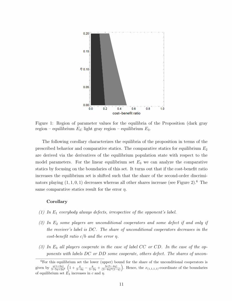
Figure 1: Region of parameter values for the equilibria of the Proposition (dark grayregion – equilibrium E2; light gray region – equilibrium E3.
The following corollary characterizes the equilibria of the proposition in terms of the
prescribed behavior and comparative statics. The comparative statics for equilibrium E2
are derived via the derivatives of the equilibrium population state with respect to the
model parameters. For the linear equilibrium set E3 we can analyze the comparative
statics by focusing on the boundaries of this set. It turns out that if the cost-benefit ratio
increases the equilibrium set is shifted such that the share of the second-order discrimi-
nators playing (1, 1, 0, 1) decreases whereas all other shares increase (see Figure 2).6 The
same comparative statics result for the error η.
Corollary
(1) In E1 everybody always defects, irrespective of the opponent’s label.
(2) In E2 some players are unconditional cooperators and some defect if and only if
the receiver’s label is DC. The share of unconditional cooperators decreases in the
cost-benefit ratio c/b and the error η.
(3) In E3 all players cooperate in the case of label CC or CD. In the case of the op-
ponents with labels DC or DD some cooperate, others defect. The shares of uncon-
6For this equilibrium set the lower (upper) bound for the share of the unconditional cooperators is
given by η(1+2η)3−5η+2η2
(
1 + 43−4η − 8
3−2η + 3c(5−4η)(3−4η)2(1−η)
)
. Hence, the x(1,1,1,1)-coordinate of the boundaries
of equilibrium set E3 increases in c and η.
11

ditional cooperators, first-order discriminators increase and (1, 1, 1, 0)-second-order
discriminators increase whereas the share of (1, 1, 0, 1)-second-order discriminators
decreases in the cost-benefit ratio c/b and the error η.
The corollary emphasizes three interesting characteristics of the cooperative equilibria.
First, they are consistent with the presence of unconditional cooperators. Second, sta-
bility requires the presence of second-order discriminators which highlights the necessity
for second-order information to sustain cooperation through indirect reciprocity. Third,
the strategy x1,1,0,1 reminds one of the well-studied reputation dynamics called standing
which always credits a sender with a good reputation except for the case in which help
was refused to a receiver with a good reputation (e.g., Ohtsuki and Iwasa, 2007). More
surprising is the prediction of the strategy (1, 1, 1, 0) which at first glance might be per-
ceived as rather unreasonable behavior. This strategy is, however, internally consistent as
it prescribes some sort of forgiving by helping when the partner did not previously help.
The refusal of help when facing label DD could be interpreted as the intention to induce
forgiving among other players. The remarkable small set of stable equilibria and their
simple structure merits some detailed reflection upon the characteristics of the involved
strategies.
Under the smallest errors of perception and implementation unconditional cooperation
uniquely maximizes the number of cooperative acts and is therefore the efficient behavior.
A homomorphic population of unconditional cooperators is, however, vulnerable to the
invasion of defectors who have a relative advantage if cooperation is non-discriminatory.
Importantly, the defectors will primarily receive the label DC as most of the time they
interact with formerly cooperative individuals. Thus, in order to discipline such defectors
and prevent an invasion unconditional cooperators need to be safeguarded by discrimi-
nating cooperators. These individuals are indeed second-order discriminators who refuse
to help if and only if they are matched with a person with a DC reputation. The re-
quired share, x(1,1,0,1), increases as cooperation becomes relatively more costly, i.e., as
CBR increases. This is because a higher share x(1,1,0,1) increases the likelihood of defec-
tors getting punished and this compensates for the relative disadvantage of cooperators
as a result of a higher CBR. Now, if the CBR further increases defection on coopera-
tive behavior eventually turns profitable. To circumvent this, punishment needs to be
intensified. Since defectors are relatively more likely to generate the DD reputation the
second-order discriminator strategy x(1,1,1,0) becomes an equilibrium strategy to back up
cooperation. As a consequence of our lemma this also introduces the first-order discrim-
inator strategy x(1,1,0,0) (see Figure 1). Finally, defection when facing the label CD can
12

never be part of a cooperative equilibrium strategy. Intuitively, defection conditional on
the label CD does not punish defectors who primarily carry labels DC and DD but only
the cooperators predominantly carrying labels CC and CD. Thus, such behavior cannot
stabilize cooperation.
Each of the pairs of parameters depicted in Figure 1 corresponds to a particular
equilibrium (set). Figure 2 illustrates the distribution over equilibrium strategies for each
pair of parameters. For the equilibrium set E3 this requires the selection of a particular
population state. In this regard, Figure 2 focuses on the center of gravity for the linear
equilibrium set E3. In line with the corollary, Figure 2 reveals that in the region associated
with equilibrium E2 the share of second-order discriminators x(1,1,0,1) increases in the cost-
benefit ratio. When this equilibrium ceases to exist the minimum level of unconditional
cooperators which can be sustained by this equilibrium is reached. The emergence of
another second-order strategy, (1, 1, 1, 0), and of the first-order discriminator (1, 1, 0, 0)
increases in the cost-benefit ratio and partially substitutes (1, 1, 0, 1). Additionally, Figure
2 indicates that the distribution of equilibrium strategies is fairly robust to errors in the
perception of labels and the implementation of strategies.
Figure 2: Left: Distribution of strategies in E2 and E3: black – x(1,1,1,1); white – x(1,1,0,1);light gray – x(1,1,0,0); dark gray – x(1,1,1,0). For E3 the center of gravity is used as arepresentative. Right: Equilibria E2 and E3 in the 3-simplex for different cost-benefitratios. The arrows indicate increasing cost-benefit ratios.
13

3 Experiment
3.1 Design of the experiment
Subjects were assigned into groups of 12, with the group being assigned either a “low” or
“high” cost of giving (c=5ECU, 10ECU). The benefit of giving was always b=25ECU .
Participants were matched in pairs within their own group over 11 periods. No two
subjects were matched together more than once, and they were made aware of this in
advance (perfect stranger matching).
In each period, participants were asked to choose between keeping or giving to their
partner. If a mover gave then his payoff was 75 ECU and that of the receiver was 40 + b
ECU. If a movers kept then his payoff was 75 + c ECU and that of the receiver was 40
ECU. The exchange rate was set at 1ECU=0.10e and participants were additionally
paid a 4e show-up fee.
In the first period, subjects were given no information about their partner. In the
second period, they were told what their partner did last period (first-order information).
In the third and subsequent periods, they were told what their partner did last period
and what their partners’ partner did in the previous-to-last period (second-order infor-
mation). We illustrated the game played and the meaning of the information given by
representing participants on the screen as shown in Figure 3 for periods 3 to 11 (equivalent
representations were shown for periods 1 and 2).
Give
OtherPerson
In period 3, you meet someone new.
You have two alternatives to choose from: “keep” or “give”.
If you choose “keep”, you will receive 85 ECU and the other person will receive 40 ECU.
If you choose “give”, you will receive 75 ECU and the other person will receive 65 ECU.
The other person has chosen "keep" in the last period, when faced with someone whom they knew had chosen "give"
Which alternative do you choose? ○ Give
○ Keep
Keep
OtherPerson
?
You
Figure 3: Visual and written representation of the game from period 3 onwards.
14
Furthermore, in order to emphasize the consequences of actions taken and help strate-
gic thinking, participants were told, using the same representation, and between each
period, what information would be given to their next partner about themselves in the
following period.
Our experiment was inspired by Bolton et al. (2005) (“BKO”) but differs in a number
of respects. BKO paid the sum of payoffs over all periods while we paid one period drawn
at random. This allowed us to isolate decisions made in each period rather than inducing
history dependence in the actions of participants. BKO told participants in each period
whether they were movers or receivers while we assigned the role of mover or receiver
ex-post: Both participants of a pair in a given period had to make a decision to give or to
keep, but only one of them would see their decision implemented at the payment stage.
This increased the amount of data collected (11 decision periods rather than 7). BKO
used direct elicitation, i.e., participants only made decisions for actual labels faced in the
experiment, while we combined both elicitation methods. We used the strategy method
(Selten, 1967) in period 5 and period 11 in order to know what action would have been
chosen for every potential reputational information. In these periods participants had to
choose an action for all four possible labels they could encounter. If one of those periods
was chosen for payment then participants were paid for the action the mover took with
respect to the actual label of the receiver. This solves the issue whereby we do not know
what strategy was played by many participants in BKO because most of them were not
faced with the full range of reputational information. We use the strategy method only
in two periods, while other periods are designed to give participants experience in playing
the game, and thus inform their answers under the strategy method.
BKO told participants how many periods they would play while we did not inform
participants of the number of periods in the experiment. This avoids the end-game effect,
with reduced giving, that occurs in BKO. Unlike BKO, we did not tell movers about the
choice made by their partner in previous periods, as this was shown to influence behavior
while it was not taken into account by the theory we are testing in this paper.
Finally, BKO chose cost-benefit ratios c/b=1/5 and c/b=3/5 while we chose ratio c/b=
1/5 and c/b=2/5. These values were chosen for several reasons. First, our model predicts
x0,0,0,0=1, that is, no giving, as the unique stable equilibrium for c/b≥1/2. The prediction
for c/b=3/5 is therefore straighforward and of little interest for us. Indeed, we are mainly
interested in CBR that are consistent with the emergence of cooperative equilibria, and
we focus on the type of strategies that sustain such equilibria. We chose c/b=1/5 to allow
a direct comparison with the results in BKO. For c/b=1/5 our model predicts E3 to be
15

the unique stable equilibrium. We will analyze whether observed strategies correspond to
the predicted set of equilibrium strategies. We further test the comparative statics in our
model by choosing another CBR, c/b=2/5, that has the same equilibrium set prediction in
terms of strategies employed, but differs in terms of the proportions of predicted strategies
in the population.
Procedure
We ran our experiment in March 2017 at the Gottingen Laboratory of Behavioral Eco-
nomics (GLOBE) in Gottingen. The experiment was computerized using the Zurich
Toolbox for Ready-made Economic Experiments (z-Tree; Fischbacher, 2007) and partic-
ipants were recruited using the Online Recruitment System for Economic Experiments
(ORSEE; Greiner, 2015). In accordance with the Declaration of Helsinki, all participants
were requested to read an online consent form and agree with its terms (by clicking) before
registering to take part in an experiment.7 Participants were guaranteed the anonymity
of the data generated during the experiment.8
We ran 7 experimental sessions with 24 participants each, for a total of 168 partici-
pants. Each session had two groups of 12, one for each treatment. In total therefore, we
observed 14 groups of 12 participants, that is, seven groups for each of the cost treat-
ments. Participants ranged in age from 18 to 51, with a mean of 25. 44% were men, 94%
German and 95% students, of which 45% studied economics. The experimental sessions
lasted approximately 90 minutes and participants earned an average of 10.70e (min =
8e, max = 12.50e). This payoff includes a 4e base payment for showing up, as well
as a payment proportional to individual payoff in one randomly selected period of the
experiment.
Payment We implemented some aspects of the PRINCE procedure (Johnson et al.,
2015) by selecting in advance of each session the period and role that would be paid for
each participant, and giving them this information on a piece of paper in a sealed envelope
at the beginning of the experiment, to be opened only at its end.9 The period was drawn
randomly, as was the role of each member of the pairs formed in that period. The sealed
envelopes were labeled with a cabin number. Subjects drew an envelope at random when
7Rules of the GLOBE are available at http://www.lab.wiwi.uni-goettingen.de/public/rules.php8The GLOBE’s privacy policy is available at http://www.lab.wiwi.uni-
goettingen.de/public/privacy.php9The paper in the envelope told them “You are a (mover/recipient). The period that will be paid is
period (number).”
16

entering the laboratory and went to the corresponding cabin. They were instructed not to
open their envelope until we gave them the signal to do so. At the end of the experiment,
and after we checked that each envelope was still closed, we gave participants the signal
to open them. Subjects then had to input the information contained in their envelope
on their computer. We checked this was done correctly before letting them proceed to
the payment stage. At that stage, along with their payoff, movers were reminded of the
action they had taken in the payment period and of the information that was available to
them about their counterpart in that period. Receivers were informed in a similar way.
The advantage of this procedure was to emphasize that the assignment to a role
and the choice of a payment period are not affected by a subject’s behavior during the
experiment. It also emphasizes that any period may be relevant, and that the role played
in that period is not known. Finally, this procedure makes it easy to explain to subjects
in what role and in what period they will be paid: we inform them of this on the paper
inside their closed envelope.
Questionnaire The experiment was followed by a socio-economic questionnaire, a mod-
ified cognitive-reflection test (Frederick, 2005), and questions about the participant’s ex-
perience and perception of the experiment. Translated instructions and a list of questions
are shown in Appendix A.5.
3.2 Hypotheses
Our theoretical results lead to two testable predictions. Equilibrium set E3 is the unique
stable equilibrium for the cost-benefit ratios in both of our treatments (see Figure 1). We
first test that the strategies used by participants correspond to those predicted by E3:
Hypothesis 1 In both treatments participants will employ one of the following strategies:
(1, 1, 1, 1), (1, 1, 1, 0), (1, 1, 0, 1), or (1, 1, 0, 0).
This hypothesis means in particular that some participants will take account of second-
order information in their choices, i.e., they will adopt different behavior when faced with
labels DC and DD. We then test comparative statics within E3 based on the Corollary
(see Figure 2), by comparing the frequency of strategies across treatments.
Hypothesis 2 The shares of unconditional cooperators (1, 1, 1, 1), first-order discrimina-
tors (1, 1, 0, 0), and (1, 1, 1, 0)-players will be higher in the high cost treatment than in the
low cost treatment, while the share of (1, 1, 0, 1)-players will be lower.
17
3.3 Results
The structure of the presentation of the experimental results is as follows. First, we
present summary statistics on directly elicited behavior and compare those with findings
in BKO. In a second step we show the consistency of direct elicitation and the strategy
method. Finally, we test our two hypotheses with data elicited from the strategy method.
3.3.1 Direct elicitation
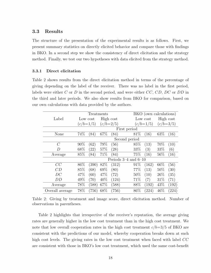
Table 2 shows results from the direct elicitation method in terms of the percentage of
giving depending on the label of the receiver. There was no label in the first period,
labels were either C or D in the second period, and were either CC, CD, DC or DD in
the third and later periods. We also show results from BKO for comparison, based on
our own calculations with data provided by the authors.
Treatments BKO (own calculations)Label Low cost High cost Low cost High cost
(c/b=1/5) (c/b=2/5) (c/b=1/5) (c/b=3/5)First period
None 74% (84) 67% (84) 81% (16) 63% (16)Second period
C 90% (62) 79% (56) 85% (13) 70% (10)D 68% (22) 57% (28) 33% (3) 33% (6)
Average 85% (84) 71% (84) 75% (16) 56% (16)Periods 3–4 and 6–10
CC 86% (390) 82% (312) 91% (162) 66% (56)CD 85% (68) 69% (80) 77% (13) 50% (30)DC 47% (60) 47% (72) 50% (10) 26% (35)DD 49% (70) 40% (124) 71% (7) 31% (71)
Average 78% (588) 67% (588) 88% (192) 43% (192)
Overall average 78% (756) 68% (756) 86% (224) 46% (224)
Table 2: Giving by treatment and image score, direct elicitation method. Number ofobservations in parentheses.
Table 2 highlights that irrespective of the receiver’s reputation, the average giving
rates are generally higher in the low cost treatment than in the high cost treatment. We
note that low overall cooperation rates in the high cost treatment c/b=3/5 of BKO are
consistent with the predictions of our model, whereby cooperation breaks down at such
high cost levels. The giving rates in the low cost treatment when faced with label CC
are consistent with those in BKO’s low cost treatment, which used the same cost-benefit
18

ratio. Other giving rates are difficult to meaningfully compare given the low number of
observations in BKO.
We observe as in BKO that label CC is dominant in the low cost treatment (66%
of observations in our experiment vs. 84% of observations in BKO). As in BKO, the
increase in the cost-benefit ratio leads to a wider variety of labels being found in the
population, whereby label CC accounts for only 53% of observations in our high cost
treatment (c/b=2/5), and 29% of observations in BKO’s high cost treatment (c/b=3/5).
With respect to the dynamics of the label distribution we observe a fast convergence
to a stable distribution of labels in both treatments which warrants the corresponding
assumption in our theoretical analysis (see Figure 4, Appendix A.3).
3.3.2 Strategy method vs. direct elicitation
From a review of literature comparing the two methods (Brandts and Charness, 2011),
we expect broad agreement in the statistics elicited under the strategy method and the
direct elicitation method. Given initial learning and the limitations in both the number
of individual observations and in the variation in receivers’ labels, particularly in the low
cost treatment, there is no meaningful test of consistency of methods on an individual
level. We therefore assess differences between elicitation methods by comparing aggregate
rates of giving by label under the strategy method (Table 3) with those elicited using the
direct elicitation method (Table 2).
Period 5 Period 11Label Low cost
(c/b=1/5)High cost(c/b=2/5)
Low cost(c/b=1/5)
High cost(c/b=2/5)
CC 87% 81% 92% 77%CD 88% 80% 82% 77%DC 38% 32% 43% 44%DD 39% 32% 42% 38%
Table 3: Giving by treatment and image score, strategy method (N=84 in each cell).
We do find that giving rates as a function of labels are not significantly different
between the strategy method and direct elicitation. The largest difference is in giving
rates when faced with label CD in the high cost treatment, which are higher under the
strategy method in period 5. This difference is, however, not significant (two-sample test of
proportions, 80% vs. 69%, p=0.106). Hence, aggregate giving rates indicate that behavior
is consistent across elicitation methods in both treatments and elicitation periods. As
outlined in the design section, the main purpose of also using the direct strategy method
19

was to give participants the opportunity to learn the game and learn their label-contingent
inclination to help which in turn allows them to formulate strategies. When turning to
the tests of our hypothesis, in the following we therefore focus on the data elicited via the
strategy method.
3.3.3 Strategy profiles
We now consider the strategy profile of our participants, which are not available in BKO
since BKO used only the direct elicitation method and many participants were never
faced with the full range of labels. We use strategies elicited using the strategy method
in the 5th period, which occurs after two periods of experience dealing with second-order
information, and in the 11th period, which is the (unannounced) last period.
Composition of strategies (Hypothesis 1) Table 4 reports the number of subjects
employing each type of strategy, with strategies labeled as in the theoretical part. We
find that the majority of subjects follow one of the four predicted equilibrium strategies.
Indeed, predicted strategies account for 85% (low cost) and 76% (high cost) of individual
strategies in period 5, and account for 81% (low cost) and 73% (high cost) of individual
strategies in period 11. We can therefore state the following result:
Result 1 In both treatments more than 3/4 of the participants follow one of the predicted
equilibrium strategies.
We consider next whether this 75% share is consistent with our hypothesis whereby
100% of participants play equilibrium strategies. In order to do so, we have to take into
account individual errors in implementation that capture unintended defection in our
model (parameter η). Such errors may lead subjects to specify off-equilibrium strategies.
We thus compute the aggregate share of the equilibrium strategies (ASES) we should
actually expect to observe given errors of implementation if we assume that all subjects
intended to play equilibrium strategies. The ASES is (1 − η)2(1 + η)2 − (α + β)(1 −η)2(1 + η)2η + (1 − η)24η2x(1,1,1,1), where α and β are defined in the proposition. This
proposition also provides upper and lower bounds on x(1,1,1,1), which we can then translate
into corresponding bounds on ASES for a given η.
20

Period 5 Period 11 Stability Stability∗
Strategy Low cost(c/b=1/5)
High cost(c/b=2/5)
Low cost(c/b=1/5)
High cost(c/b=2/5)
Low cost(c/b=1/5)
High cost(c/b=2/5)
Low cost(c/b=1/5)
High cost(c/b=2/5)
1111 21 20 23 25 18/21 19/20 21/21 20/201110 10 5 13 6 7/10 2/5 10/10 4/51101 10 6 11 5 8/10 4/6 10/10 6/61100 30 33 21 25 17/30 21/33 25/30 29/33Total inequilibrium set
71 64 68 61 50/71 46/64 66/71 59/64
1010 0 1 0 2 0/0 0/1 0/0 0/11001 0 0 1 0 0/0 0/0 0/0 0/01000 2 3 8 2 2/2 0/3 0/2 1/30110 0 0 0 1 0/0 0/0 0/0 0/00101 1 0 0 0 0/1 0/0 1/1 0/00100 2 3 1 3 0/2 0/3 0/2 0/30011 1 1 0 2 0/1 0/1 1/1 0/10010 0 0 0 1 0/0 0/0 0/0 0/00000 7 12 6 12 5/7 10/12 0/7 1/12Total not inequilibrium set
13 20 16 23 7/13 10/20 2/13 2/20
Total 84 84 84 84 57/84 56/84 68/84 61/84Stability∗: Maintain strategy or switch within equilibrium strategy set.
Table 4: Distribution and stability of strategies across treatments.
21

We estimate individual implementation error η by comparing answers by our partici-
pants in periods 5 and 11 to what they did in periods 4 and 10. Participants received no
new information about the distribution of labels between periods 4 and 5, and between
periods 10 and 11, as they received no second-order information about their randomly
assigned partner in periods 5 and 11. They therefore had the same information as in
periods 4 and 10, respectively, so that differences in the decision to help in period 4
(10) for a given observed label and the decision in period 5 (11) for that label is a good
measure of possible implementation errors. The average error rate, η, was 7.5% when
aggregating over treatments and periods (Table A.4 in the Appendix). The 95% exact
(Clopper-Pearson) binomial confidence interval for this statistic is [4.5%, 11.5%].
Given the above confidence interval estimate for η, we obtain an average ASES of
about 71% with a confidence interval of [55%, 82%] for both treatments. Hence, the
share of participants who are observed playing equilibrium strategies in our experiment is
consistent with our measure of implementation errors and the hypothesis that every player
adheres to one of the predicted equilibrium strategies. Note that while individual errors
of implementation can account for the infrequent observation of most off-equilibrium
strategies, the observed share of unconditional defectors is higher than what could be
explained with implementation errors alone. We elaborate on this in our discussion.
Comparison across treatments (Hypothesis 2) We now compare the frequency
of different types of strategies across treatments. We can reject the hypothesis that
the frequency of use of strategies does not differ across treatments, either in period 5
(Pearson’s χ2=10.44, p=0.034) or in period 11 (Pearson’s χ2=18.30, p=0.001). There
are therefore significant differences in the distribution of strategies across treatments.
p(sL>sH)Strategy Period 5 Period 111111 57% 37%1110 91% 95%1101 84% 94%1100 31% 24%
Table 5: Posterior probabilities, p, that proportions in the low cost treatment, sL, arehigher than in the high cost treatment (sH).
We perform a Bayesian estimation of a model of multinomial proportions over all
strategies, so as to express posterior probabilities that the difference in the proportions of
each strategy across treatments are greater than zero (Table 5). We find that the share
22
of unconditional cooperators and first-order discriminators is likely to be equal or higher
in the high cost treatment than in the low cost treatment in period 11, while the share of
(1, 1, 0, 1)-players is likely to be lower. This is consistent with Hypothesis 2. In contrast
to our prediction, the share of (1, 1, 1, 0)-players, however, is likely to be lower in the high
cost treatment. Overall, we can state the following result:
Result 2 The mix of strategies followed by participants differs across treatment. Three
out of 4 of the differences in the frequency of strategies are consistent with Hypothesis 2.
Stability of strategy choices We test the stability of equilibrium E3 by considering
whether there are fewer changes of strategies between periods 5 and 11 by participants who
follow equilibrium strategies than by participants who follow non-equilibrium strategies.
As a first indication of overall stability, a multinomial chi-square test of frequencies cannot
reject the hypothesis that there is no change in the frequencies of strategies from period
5 to period 11, either in the low cost treatment (Pearson’s χ2=5.38, p=0.251) or in the
high cost treatment (Pearson’s χ2=4.32, p=0.365).10 There are therefore only limited
changes in the mix of strategies over time in both treatments.
We then analyze whether participants who adopt strategies that correspond to our
predictions do so with more consistency than individuals who adopt other strategies.
If this is so, this allows us to argue that other strategies correspond to mistakes by
participants or to an unfinished learning process. The two columns labeled “stability”
in Table 4 show how many participants use the same strategy in period 11 as in period
5. Overall, about 2/3 of participants in both treatments maintained the same strategy
from period 5 to period 11. We find that strategies in the equilibrium set are more robust
than those outside of it (70% stability within vs. 54% stability outside in the low cost
treatment; 72% stability within vs. 50% stability outside in the high cost treatment).
This finding is further strengthened when considering how many participants maintain
strategies within the equilibrium set or switch within such strategies from period 5 to
period 11 (last two columns in Table 4). Overall, 93% of those who employ a strategy
within the equilibrium set in period 5 still do so in period 11 in the low cost treatment,
and 94% in the high cost treatment. The corresponding stability for non-equilibrium
strategies other than (0, 0, 0, 0) is about 40% in both treatments, which is substantially
lower. Participants who play the non-equilibrium strategy (0, 0, 0, 0), however, are also
highly likely to keep doing so: 71% do so in the low cost treatment, and 83% in the high
cost treatment. We summarize these insights in an additional result.
10We assign all non-equilibrium strategies other than unconditional defection to the same category.
23

Result 3 Participants who use predicted equilibrium strategies do so in a more consistent
way than those who apply off-equilibrium strategies. Unconditional defectors, however,
are also consistent in their use of their strategy.
4 Discussion
Since the mechanism of indirect reciprocity has predominantly been studied in the bi-
ological literature, we briefly discuss our theoretical findings in light of this strand of
literature. In that literature, it is usually assumed that each player has a binary repu-
tation score, either good or bad. This reputation is observable by all other players and
each player applies a behavioral strategy that prescribes the behavior for each reputation
score. A large part of the literature studied the dynamics of the behavioral strategies
under the assumption that the whole population shares the same social norm, i.e., there
is an agreement on what is good and what is bad. Partially, this assumption is made for
technical reasons. If multiple social norms coexist then a player might be considered bad
by some and good by some others, which makes the analysis of the reputation dynamics
almost intractable.
One of the most comprehensive studies in this literature is Ohtsuki and Iwasa (2004).
They present an exhaustive analysis of all reputations dynamics that assign a binary rep-
utation (good or bad) to each player when his action, his current reputation, and the
opponent’s reputation are given. They identify and characterize eight reputation dynam-
ics, which they name the “leading eight,” that can maintain a high level of cooperation.
As a common characteristics, they share the property that, for someone with a good rep-
utation, helping is considered to be good behavior whereas refusing to help is thought
of as bad. They also share the characteristic that refusal to help a bad individual does
not undermine the reputation of a good person. The “leading eight” do not, however,
all agree in their evaluation of a behavior that was undertaken by a person with a bad
reputation. The leading eight differ mostly in the way in which helping someone with a
bad reputation is evaluated.
We refrained from making the assumption of an universally shared social norm in
society and focused on the coevolution of strategies that can condition on some recent
histories of the game. Note that a player may cooperate for different reasons. Cooperation
may not only reflect some normative judgment of the opponent’s past behavior but it
may also involve strategic reasoning regarding the reaction of other players in the future.
However, under the assumption that a player’s cooperative act can be interpreted as a
24
moral judgment of the opponent’s past play our results can be interpreted as an analysis of
the coevolution of social norms under indirect reciprocity. In light of this interpretation,
the aforementioned commonalities of the leading eight correspond to strategies which
cooperate in the case of the label CC and refuse to help in the case of DC, which is the
case for all of our conditional cooperative equilibrium strategies. Interestingly, the fact
that all equilibrium strategies prescribe cooperation in the case of the label CD points
toward two particular reputation systems among the leading eight.11 The first is known
as the “standing strategy” first proposed by Sugden (1986). The second differs from
standing by always assigning a good reputation to someone who refuses to help a bad
person. Thus, based on our results we may conjecture that a coevolutionary analysis of
the leading eight reputation dynamics would reveal a particular role of these two systems.
Due to the aforementioned difficulties of a coevolutionary analysis there is only one
recent study on this topic. Yamamoto et al. (2017) show with agent-based simulations
that after cooperation is achieved four strategies coexist. These four strategies are exactly
those four strategies constituting equilibrium set E3.12 Thus, our theoretical results may
provide the analytic foundation of their simulation results.
Finally, as highlighted by our first experimental result, in light of individual imple-
mentation errors we cannot reject the hypothesis that all players adhere to one of the
predicted equilibrium strategies. Although implementation errors can account for the
infrequent occurrence of most non-equilibrium strategies, they fail to rationalize the sig-
nificant and stable share of unconditional defectors. This might indicate that our theory
misses a relevant driver for the participants’ strategic and moral considerations or might
simply reflect a player who did not fully grasp the structure of the game. The latter
might induce unconditional defection as the direct rewards from defection are easier to
comprehend than the uncertain and indirect benefits from cooperation.
5 Conclusion
In this paper we present an analytically tractable evolutionary model of indirect reci-
procity and provide evidence from a laboratory experiment. Instead of assuming that each
societal member abides by the same reputation mechanism, we analyze the coevolution of
strategies that differ in how they condition on publicly available second-order information
about opponents’ past behavior. We fully characterize the evolutionary stable equilibria
11In the model of Ohtsuki and Iwasa (2004) this would be captured by d∗0C=1.12In the notation of Yamamoto et al. (2017) these strategies are (GGGG), (GGBG), (GGGB), and
(GGBB).
25

in this game and study their comparative statics with respect to the cost-benefit ratio.
Surprisingly, there exist only two stable cooperative equilibria in the 15-dimensional pop-
ulation state space. These equilibria are also of low complexity, the first is a population
state constituted by two strategies, the second is a linear set of population states with two
additional strategies. In our laboratory experiment we employed the strategy method to
gain full information about participants’ strategies and we implemented two treatments
with different cost-benefit ratios. More than 75% of the participants’ elicited strategies
correspond to one of the four predicted equilibrium strategies. Moreover, most differences
in the distribution of strategies across treatments were in line with our predictions.
The theoretical results and the experimental evidence regarding the presence of strate-
gies which rely on second-order information reemphasize the relevance of higher-order
information to promote cooperation under indirect reciprocity. Our results highlight the
importance of the coevolutionary perspective as we find no cooperative equilibrium con-
stituted by a homomorphic population. We also shed some light on the issue of selection
among different reputation mechanisms. We identify a particularly important strategy
which is present in both equilibria and discriminates based on second-order information.
This strategy only punishes a partner who behaved non-cooperatively toward a formerly
cooperative subject. It prescribes cooperation, however, if the current partner’s non-
cooperative behavior is justifiable in the sense that his former opponent defected himself.
Thus, our results indicate that the reputation mechanism known as “standing” which
was first proposed by Sugden (1986) and identified as one of the “leading eight” by Oht-
suki and Iwasa (2004) is of particular importance for the evolution of cooperation under
indirect reciprocity.
This finding may explain the design of a well-documented historical example of a
reputation system which relied on second-order information (Greif, 1989). In the 11th
Century a group of Mediterranean traders relied on agents to complete some of their
business dealings abroad. The immanent moral hazard problem was solved via an informal
reputation mechanism described by Greif as follows. “[A]ll coalition merchants agree never
to employ an agent that cheated while operating for a coalition member. Furthermore, if
an agent who was caught cheating operates as a merchant, coalition agents who cheated
in their dealings with him will not be considered by other coalition members to have
cheated.” That is, cheating on someone who cheated was not punished.
Finally, given that players’ strategies at least partially reflect the moral judgment of
their opponents’ past behavior, the fact that all cooperative equilibria are constituted by
a heteromorphic population offers an explanation for the omnipresent heterogeneity in
26

moral judgments among humans (e.g., Haidt et al., 2009; Weber and Federico, 2013).
References
Alexander, R.D., 1987. The biology of moral systems. Aldine de Gruyter, New York.
Alger, I., Weibull, J.W., 2013. Homo moralis – Preference evolution under incomplete
information and assortative matching. Econometrica 81, 2269–2302.
Berger, U., 2011. Learning to cooperate via indirect reciprocity. Games and Economic
Behavior 72, 30–37.
Berger, U., Grune, A., 2016. On the stability of cooperation under indirect reciprocity
with first-order information. Games and Economic Behavior 98, 19–33.
Bergstrom, T., 2009. Ethics, evolution, and games among neighbors. Working Paper.
University of California, Santa Barbara.
Bolton, G.E., Katok, E., Ockenfels, A., 2005. Cooperation among strangers with limited
information about reputation. Journal of Public Economics 89, 1457–1468.
Brandts, J., Charness, G., 2011. The strategy versus the direct-response method: a
first survey of experimental comparisons. Experimental Economics 14, 375–398. URL:
https://doi.org/10.1007/s10683-011-9272-x, doi:10.1007/s10683-011-9272-x.
Charness, G., Du, N., Yang, C.L., 2011. Trust and trustworthiness reputations in an
investment game. Games and Economic Behavior 72, 361–375.
Fischbacher, U., 2007. z-Tree: Zurich toolbox for ready-made economic experiments.
Experimental Economics 10, 171–178.
Frederick, S., 2005. Cognitive reflection and decision mak-
ing. Journal of Economic Perspectives 19, 25–42. URL:
https://www.aeaweb.org/articles?id=10.1257/089533005775196732,
doi:10.1257/089533005775196732.
Greif, A., 1989. Reputation and coalitions in medieval trade: Evidence on the Maghribi
traders. Journal of Economic History 49, 857–882.
Greiner, B., 2015. Subject pool recruitment procedures: Organizing experiments with
ORSEE. Journal of the Economic Science Association 1, 114–125.
27
Haidt, J., Graham, J., Joseph, C., 2009. Above and below left–right: Ideological narratives
and moral foundations. Psychological Inquiry 20, 110–119.
Heller, Y., Mohlin, E., 2017. Observations on cooperation. Review of Economic Studies
85, 2253–2282.
Johnson, C.A., Baillon, A., Bleichrodt, H., Li, Z., Van Dolder, D., Wakker, P.P., 2015.
Prince: An improved method for measuring incentivized preferences. SSRN Schol-
arly Paper ID 2504745. Social Science Research Network. Rochester, NY. URL:
https://papers.ssrn.com/abstract=2504745.
Kandori, M., 1992. Social norms and community enforcement. Review of Economic
Studies 59, 63–80.
Nowak, M.A., 2006. Five rules for the evolution of cooperation. Science 314, 1560–1563.
Nowak, M.A., Sigmund, K., 1998. Evolution of indirect reciprocity by image scoring.
Nature 393, 573.
Ohtsuki, H., Iwasa, Y., 2004. How should we define goodness? Reputation dynamics in
indirect reciprocity. Journal of Theoretical Biology 231, 107–120.
Ohtsuki, H., Iwasa, Y., 2006. The leading eight: Social norms that can maintain cooper-
ation by indirect reciprocity. Journal of Theoretical Biology 239, 435–444.
Ohtsuki, H., Iwasa, Y., 2007. Global analyses of evolutionary dynamics and exhaustive
search for social norms that maintain cooperation by reputation. Journal of Theoretical
Biology 244, 518–531.
Okuno-Fujiwara, M., Postlewaite, A., 1995. Social norms and random matching games.
Games and Economic Behavior 9, 79–109.
Panchanathan, K., Boyd, R., 2003. A tale of two defectors: The importance of standing
for evolution of indirect reciprocity. Journal of Theoretical Biology 224, 115–126.
Seinen, I., Schram, A., 2006. Social status and group norms: Indirect reciprocity in a
repeated helping experiment. European Economic Review 50, 581–602.
Selten, R., 1967. Die Strategiemethode zur Erforschung des eingeschrankt rationalen
Verhaltens im Rahmen eines Oligopolexperiments, in: Sauermann, H. (Ed.), Beitrage
zur Experimentellen Wirtschaftsforschung. Tubingen: J.C.B. Mohr. volume 1, pp. 136–
168.
28

Sugden, R., 1986. The economics of rights, co-operation and welfare. Blackwell, Oxford,
UK.
Takahashi, S., 2010. Community enforcement when players observe partners’ past play.
Journal of Economic Theory 145, 42–62.
Trivers, R.L., 1971. The evolution of reciprocal altruism. Quarterly Review of Biology
46, 35–57.
Weber, C.R., Federico, C.M., 2013. Moral foundations and heterogeneity in ideological
preferences. Political Psychology 34, 107–126.
Yamamoto, H., Okada, I., Uchida, S., Sasaki, T., 2017. A norm knockout method on
indirect reciprocity to reveal indispensable norms. Scientific Reports 7, 44146.
29

A Appendices
A.1 Proofs
Lemma.
Inserting the definition of pC(s) and pC(s, s′) into the definition of profits given by equation
(10) gives us:
Πs(τ ; c, η)−Πs′(τ ; c, η)=∑
s
xs(τ)(
pC(s, s)−pC(s, s′))
− c
2
(
pC(s)−pC(s′))
(A.1)
=1
2
∑
s
xs(τ)(
ps|CC(pCC|s−pCC|s′)+. . .+ps|DD(pDD|s−pDD|s′))
− c
2
(
(ps|CC−ps′|CC)pCC+. . .+(ps|DD−ps′|DD)pDD
)
(A.2)
Inserting equations (2)–(5),
=1
2
∑
s
xs(t)(
ps|CC(ps|CC−ps′|CC)pCC+. . .+ps|DD(ps|DD−ps′|DD)pDD
)
− c
2
(
(ps|CC−ps′|CC)pCC+. . .+(ps|DD−ps′|DD)pDD
)
(A.3)
Inserting (1),
=b
2
∑
s
xs(τ)(
ps|CC
(
(s1−s′1)(1−η)+. . .+(s4−s′4)η
3
)
(1−η)pCC+. . .
+ps|DD
(
(s4−s′4)(1−η)+. . .+(s1−s′1)η
3
)
(1−η)pDD
)
− c
2
(
(
(s1−s′1)(1−η)+. . .+(s4−s′4)η
3
)
(1−η)pCC+. . .
+(
(s4−s′4)(1−η)+. . .+(s1−s′1)η
3
)
pDD
)
(A.4)
30

Collecting the terms (si−s′i),
=1
2
(
(s1−s′1)(1−η)(
(1−η)pCC
∑
s
xs(τ)ps|CC+. . .+η
3pDD
∑
s
xs(τ)ps|DD
)
+. . .
+(s4−s′4)(1−η)(
pCCη
3
∑
s
xs(τ)ps|CC+. . .+(1−η)pDD
∑
s
xs(τ)ps|DD
)
)
− c
2
(
(s1−s′1)(1−η)(
(1−η)pCC+η
3pCD+
η
3pDC+
η
3pDD
)
+. . .
+(s4−s′4)(1−η)(η
3pCC+
η
3pCD+
η
3pDC+(1−η)pDD
)
)
(A.5)
Applying the definition of the four basic payoff differences,
=4
∑
i=1
(si−s′i)∆Πi(τ ; c, η) (A.6)
Proposition.
The proof proceeds in two steps. In step one we show that for 26 of the 30 potentially
stable equilibria presented in Table 1 there are non-equilibrium strategies yielding strictly
higher payoffs contradicting asymptotic stability. The 30 candidates were derived with
the help of Mathematica 10 (see supplementary). In step two we analyze each of the
remaining equilibria separately.
Step One
1. {(xs)|s∈S}For each of the 16 cases we analyze the profits of strategy s under the condition that
xs=1. It turns that population states with xs=1 for s∈{(1, 1, 1, 1), (1, 0, 1, 1), (0, 1, 1, 1),(1, 0, 1, 0), (0, 1, 0, 1), (0, 0, 1, 1), (1, 0, 0, 1), (0, 0, 1, 0), (0, 0, 0, 1)} are vulnerable for in-vasions by all defectors, i.e., by strategy (0, 0, 0, 0).
Let ∆Πs=(
Πs(τ, c, η)− Π(0,0,0,0)(τ, c, η))∣
∣
xs=1. Payoff differences are given by
∆Π(1,1,1,1)=−(1− η), ∆Π(1,0,1,1)=− (3−η)(1−η)(12−31η+23η2−4η3+3c(7−4η))3c(9+12η−31η2+23η3−4η4)
,
∆Π(0,1,1,1)=− (3−η)(1−η)((1−η)2(9−15η+4η2)+3c(6−7η+4η2))3c(27−54η+55η2−23η3+4η4)
, ∆Π(1,0,1,0)=−2(1−η)7−4η
,
∆Π(0,1,0,1)=− (1−η)(3−2η)6−7η+4η2
, ∆Π(0,0,1,1)=− (1−η)(3−2η)(3+3c−7η+4η2)3c(6−7η+4η2)
,
∆Π(1,0,0,1)=− (1−η)(3−2η)(3+c(7−4η)−7η+4η2)c(51−94η+68η2−16η3)
, ∆Π(0,0,1,0)=− (1−η)(9c+(1−η)2η(3−4η)3c(24−22η+11η2−4η3)
31

∆Π(0,0,0,1)=− (1−η)2(9+9c−24η+22η2−11η3+4η4)c(27−45η+34η2−11η3+4η4)
. By inspection, c∈(0, 1) and η∈(0, 15) im-
ply that all these differences are strictly negative. Moreover, population states with
xs=1 for s∈{(1, 1, 1, 0), (1, 1, 0, 1), (0, 1, 1, 0)} are also vulnerable to invasions.
Π(1,1,1,0)−Π(0,0,1,1)=− (1−η)(3c(27−102η+143η2−58η3+8η4)+2η(72−342η+589η2−447η3+144η4−16η5))9c(9+19η−23η2+4η3)
,
Π(1,1,0,1)−Π(1,1,1,0)=− (4−η)η2(3−η−10η2+8η3)3(9+12η−31η2+23η3−4η4)
, Π(0,1,0,0)−Π(1,0,0,0)=− (1−η)2η2(15−26η+8η2)3(9+3η−10η2+11η3−4η4)
Π(0,1,1,0)−Π(1,0,1,0)=−2(1−η)2η(3−4η)(3+3c−7η+4η2)3c(3−2η)(11−10η+8η2)
. Again, all these differences are neg-
ative. Thus, the remaining candidates are the strategies (1, 1, 0, 0) and (1, 0, 0, 0).
Regarding the former, note that Π(1,1,0,0) − Π(1,0,1,0)=0 for population states with
x(1,1,0,0) + x(1,0,1,0)=1. Hence, the population state x(1,1,0,0)=1 cannot be stable as
an equilibrium point. In the case of the latter, it turns out that either (1, 1, 0, 0) or
(0, 0, 0, 0) earns strictly higher payoffs in a population state with x(1,0,0,0)=1. First,
Π(1,0,0,0)−Π(1,1,0,0)=− (1−η)η(2(1−η)3(9−4η)(3−4η)−3c(36−η(53−34η+8η2)))9c(18−η(2+η(11−4η)))
. Second, Π(1,0,0,0)−Π(0,0,0,0)=− (1−η)η(21−12η−((1−η)2(3−4η))/c)
54−3η(2+η(11−4η)). In sum, only the population state x(0,0,0,0)=
1 may constitute a stable equilibrium point.
2. (x(1,1,0,1), x(0,1,0,1))
It turns out that under the assumption of equal profits for strategies (1, 1, 0, 1)
and (0, 1, 0, 1) a state characterized by x(1,1,0,1) + x(0,1,0,1)=1 is vulnerable to an
invasion by strategy (1, 1, 1, 0). Under the restriction to η∈(0, 15), the condition
x(1,1,0,1)∈(0, 1) reduces to c∈(
0, (3−η)(1−η)2(3−4η)(9−(3−η)η(7−4η))3(27−η(99−η(174−η(143−58η+8η2))))
)
. In this range of cost-
benefit ratios the payoff difference Π(1,1,0,1) − Π(1,1,1,0) is strictly negative.
3. (x(1,0,0,0), x(0,0,0,0))
It turns out that under the assumption of equal profits for strategies (1, 0, 0, 0)
and (0, 0, 0, 0) a state characterized by x(1,0,0,0) + x(0,0,0,0)=1 is vulnerable to an
invasion by strategy (1, 1, 0, 0). Under the restriction to η∈(0, 15), the condition
x(1,0,0,0)∈(0, 1) reduces to c∈(
0, (1−η)2(3−4η)3(7−4η)
)
. In this range of cost-benefit ratios the
payoff difference Π(1,0,0,0) − Π(1,1,0,0) is strictly negative.
4. (x(1,1,0,1), x(1,0,0,1))
It turns out that under the assumption of equal profits for strategies (1, 1, 0, 1) and
(1, 0, 0, 1) a state characterized by x(1,1,0,1) + x(1,0,0,1)=1 is vulnerable to an invasion
by strategy (1, 1, 1, 0). Under the restriction to η∈(0, 15), the condition x(1,1,0,1)∈
(0, 1) reduces to c∈(
(1−η)(3−4η)(45−2η(81−2η(46−η(23−4η))))9(15−η(31−η(23−4η)))
, (3−η)(1−η)3(15−4η)(3−4η)9(15−η(31−η(23−4η)))
)
. In
this range of cost-benefit ratios the payoff difference Π(1,1,0,1) − Π(1,1,1,0) is strictly
negative.
32

5. (x(0,1,0,0), x(0,0,0,0))
It turns out that under the assumption of equal profits for strategies (0, 1, 0, 0)
and (0, 0, 0, 0) a state characterized by x(0,1,0,0) + x(0,0,0,0)=1 is vulnerable to an
invasion by strategy (1, 1, 0, 1). Under the restriction to η∈(0, 15), the condition
x(0,1,0,0)∈(0, 1) reduces to c∈(
0, (1−η)(3−4η)(3−η(1−η))3(6−η(7−4η))
)
. In this range of cost-benefit
ratios the payoff difference Π(0,1,0,0) − Π(1,1,0,1) is strictly negative.
6. (x(1,1,1,1), x(1,1,0,1))
It turns out that there are parameter constellations, for instance, (c= 18, η= 3
32) such
that the equilibrium strategies (1, 1, 1, 1) and (1, 1, 0, 1) earn the same and strictly
highest payoff in a state characterized by x(1,1,1,1) + x(1,1,0,1)=1. Thus, this equilib-
rium is a candidate to be considered in step two.
7. (x(1,1,1,0), x(1,1,0,0))
It turns out that under the assumption of equal profits for strategies (1, 1, 1, 0)
and (1, 1, 0, 0) a state characterized by x(1,1,1,0) + x(1,1,0,0)=1 is vulnerable to an
invasion by strategy (0, 0, 0, 0). Under the restriction to η∈(0, 15), the condition
x(1,1,1,0)∈(0, 1) reduces to c∈(
(1−η)(3−4η)(4−η)(9−2η(7−4η))3(45−2η(37−η(23−4η)))
, (1−η)(3−4η)3
)
. In this range of
cost-benefit ratios the payoff difference Π(1,1,1,0) − Π(0,0,0,0) is strictly negative.
8. (x1,0,1,0, x1,0,0,0)
It turns out that under the assumption of equal profits for strategies (1, 0, 1, 0)
and (1, 0, 0, 0) a state characterized by x(1,0,1,0) + x(1,0,0,0)=1 is vulnerable to an
invasion by strategy (1, 1, 0, 1). Under the restriction to η∈(0, 15), the condition
x(1,1,1,0)∈(0, 1) reduces to c∈(
(1−η)2η(3−4η)(7−4η)3(36−η(53−34η+8η2)
, 5763−4η
− 21 − 27(1−η)2
− 1441−η
+ 26η −8η2 −
√θ)
, where θ= 3η2(7−4η)3(10−η(11−4η))(6−η(7−4η))(3−4η)2(1−η)4
. In this range of cost-benefit
ratios the payoff difference Π(1,0,1,0) − Π(1,1,0,1) is strictly negative.
9. (x0,1,1,0, x0,1,0,0)
It turns out that under the assumption of equal profits for strategies (0, 1, 1, 0)
and (0, 1, 0, 0) a state characterized by x(0,1,1,0) + x(0,1,0,0)=1 is vulnerable to an
invasion by strategy (0, 0, 0, 0). Under the restriction to η∈(0, 15), the condition
x(1,1,1,0)∈(0, 1) reduces to c∈(
(1−η)(3−4η)(3−4η(1−η))9
, (1−η)(3−4η)(3−η(1−η))9
)
. In this range
of cost-benefit ratios the payoff difference Π(0,1,1,0) − Π(0,0,0,0) is strictly negative.
10. (x1,1,1,1, x1,1,1,0)
It turns out that under the assumption of equal profits for strategies (1, 1, 1, 1)
and (1, 1, 1, 0) a state characterized by x(1,1,1,1) + x(1,1,1,0)=1 is vulnerable to an
33

invasion by strategy (0, 0, 0, 0). Under the restriction to η∈(0, 15), the condition
x(1,1,1,1)∈(0, 1) reduces to c∈(
0, 4(1−η)(3−4η)(4−η)57−12η
)
. In this range of cost-benefit ratios
the payoff difference Π(1,1,1,1) − Π(0,0,0,0) is strictly negative.
11. (x(1,1,1,0), x(1,0,1,0), x(0,1,1,0), x(0,0,1,0))
It turns out that under the assumption of equal profits for strategies x(1,1,1,0),
x(1,0,1,0), x(0,1,1,0), and x(0,0,1,0) a state characterized by x(1,1,1,0)+x(1,0,1,0)+x(0,1,1,0)+
x(0,0,1,0)=1 is vulnerable to an invasion by strategy (1, 1, 0, 1). See supplementary
for details.
12. (x(1,1,0,1), x(0,1,0,1), x(1,0,0,1), x(0,0,0,1))
It turns out that under the assumption of equal profits for strategies x(1,1,0,1),
x(0,1,0,1), x(1,0,0,1), and x(0,0,0,1) a state characterized by x(1,1,0,1)+x(0,1,0,1)+x(1,0,0,1)+
x(0,0,0,1)=1 is vulnerable to an invasion by strategy (0, 0, 0, 0). See supplementary
for details.
13. (x(1,1,1,1), x(1,1,1,0), x(1,1,0,1), x(1,1,0,0))
It turns out that there exist parameter constellations, for instance (c= 13, η= 1
8) such
that the equilibrium strategies earn the same and strictly highest payoffs in a state
characterized by x(1,1,1,1) + x(1,1,1,0) + x(1,1,0,1) + x(1,1,0,0)=1. Thus, this equilibrium
set is a candidate to be considered in step two.
14. (x(0,1,1,1), x(0,1,1,0), x(0,1,0,1), x(0,1,0,0))
It turns out that under the assumption of equal profits for strategies x(0,1,1,1),
x(0,1,1,0), x(0,1,0,1), and x(0,1,0,0) a state characterized by x(0,1,1,1)+x(0,1,1,0)+x(0,1,0,1)+
x(0,1,0,0)=1 is vulnerable to an invasion by strategy (0, 0, 0, 0). See supplementary
for details.
15. (x(1,1,1,1), ..., x(0,0,0,0))
By definition, in this equilibrium all 16 earn the same payoff. Consequently, there
cannot exist a strategy that yields higher payoffs than the equilibrium strategies.
However, there exists a subset of this equilibrium set which is unstable such that
the neutral drift will eventually shift the population state into that region. The set
of population states which satisfy ∆Πi(τ ; c, η)=0, ∀i is given by{
x∈∆15
∣
∣
∑
s∈S
xs=
1, x(0,1,0,0)=γ+∑
s∈S2
xs−∑
s∈S3
xs, x(0,0,1,0)=−γ+∑
s∈S4
xs−∑
s∈S5
xs
}
, where γ= 3c(1−η)(3−4η)
,
S2={x(1,0,1,1), x(0,0,1,1), x(1,0,0,1), x(0,0,0,1)}, S3={x(1,1,1,0), x(1,1,0,0), x(0,1,1,0)},S4={x(1,1,0,1), x(1,1,0,0), x(1,0,0,1), x(1,0,0,0)}, S5={x(0,1,1,1), x(0,0,1,1), x(0,1,1,0)}. Consider,
34

for instance, the solution x(1,1,0,0)=3c
3−7η+4η2, x(0,0,0,0)=1 − 3c
3−7η+4η2, xs=0, ∀s∈S \
{(1, 1, 0, 0), (0, 0, 0, 0)} which satisfies the conditions for existence of this equilib-
rium, i.e., it solves ∆Πi(τ ; c, η)=0, ∀i. It turns out that with the exception of one
strictly positive eigenvalue all other eigenvalues are zero. This eigenvalue is given
by 2cη(3(1−c)−7η+4η2)2(1−η)(3−4η)
.
Taken together there are three candidates for stable (sets of) population states. The
stability of those candidates is analyzed in detail below.
Step Two
1. x(0,0,0,0)
This equilibrium is stable for all pair of parameters, i.e., for cb∈(0, 1) and η∈(0, 1
5).
This is because all other strategies earn strictly negative payoffs while (0, 0, 0, 0)
earns a payoff of zero. This results from the assumptions that there is no unin-
tended help but only unintended defection and that there are observational errors.
Thus, any strategy which prescribes cooperation for some label will eventually in-
duce cooperation because either this label is present in the population or some
other is misperceived as this particular label. As a consequence, individuals play-
ing a strategy different from (0, 0, 0, 0) will bear the cost of cooperation with some
probability but will never receive help in a state with x(0,0,0,0)=1.
2. (x(1,1,1,1), x(1,1,0,1))
Note first that this equilibrium point is internally stable in the sense that an in-
crease in the share of x(1,1,1,1) decreases the payoffs of (1, 1, 1, 1) relative to (1, 1, 0, 1)
(see supplementary). Second, as a necessary condition for stability we must have
that ∆Πi(t; c, η)>0, i 6=3. This guarantees that a deviation from cooperation for
labels CC, CD, or DD is not profitable. Taken together with the requirement that
x(1,1,1,1)∈(0, 1) this reduces to cb∈(
0, 3−10η+8η2
15−22η+8η2
)
and η∈(0, 15). To establish suffi-
ciency we study the eigenvalues of the linearized system at this equilibrium point.
Analytic solutions are presented in the supplementary. It turns out that the condi-
tions cb∈(
0, 3−10η+8η2
15−22η+8η2
)
and η∈(0, 15) imply that all eigenvalues are strictly negative,
which establishes the sufficiency of these conditions.
3. (x(1,1,1,1), x(1,1,1,0), x(1,1,0,1), x(1,1,0,0))
The condition of being well-defined, i.e., (x(1,1,1,1), x(1,1,1,0), x(1,1,0,1), x(1,1,0,0))∈∆3,
reduces with respect cband η to c
b∈[
3−10η+8η2
15−22η+8η2, 12−52η+72η2−32η3
15−22η+8η2
]
and η∈(0, 15). As
35

a necessary condition for stability we must have that ∆Πi(t; c, η)>0, i=1, 2. This
guarantees that a deviation from cooperation for labels CC, or CD is not profitable.
Taken together with the condition for existence we obtain cb∈[
3−10η+8η2
15−22η+8η2, 3−10η+8η2
6−4η
)
and η∈(0, 15). Note that at the lower bound of c
bthe equilibria (2) and (3) coincide.
That is, the equilibrium set reduces to an equilibrium point with x(1,1,1,1)+x(1,1,0,1)=
1.
To establish sufficiency we study the eigenvalues of the linearized system at a point
in this equilibrium. It turns out that there is a eigenvalue of zero with multi-
plicity one, three eigenvalues with multiplicity four, and two non-zero eigenvalues
with multiplicity one. The eigenvalue of zero with multiplicity one corresponds
to the dimension of the equilibrium set and reflects the vanishing payoff differ-
ences for the equilibrium strategies. In other words, the corresponding eigenvec-
tor (1,−1,−1, 0, 0, 1, 0, ..., 0)′
spans this equilibrium set. Note that the equilib-
rium set connects two facets of 3-simplex. Particularly, at the population state
with the minimal share of unconditional cooperators(
x(1,1,1,1)=η(1+2η)
3−5η+2η2
)
we have
x(1,1,0,0)=0, at the population state that maximizes the share of unconditional coop-
erators(
x(1,1,1,1)=1 + 43−4η
− 83−2η
+ 3c(5−4η)(3−4η)2(1−η)
)
the share x(1,1,1,0) vanishes. Thus,
the eigenvalue of zero does not cause any issue of instability at the boundaries of
this equilibrium set.
The three eigenvalues with multiplicity four are: e2−5=2(1−η)2(6−4η−
3−2η(5−4η)c
)
(3−2η)(3+6η−8η2), e6−9=
2(1−η)2η(6−4η−3−2η(5−4η)
c)(5−4η)
3(3−2η)(3+6η−8η2), and e10−13=
2(1−η)2(6−4η−3−2η(5−4η)
c)(3−5η−4η2)
3(3−2η)(3+6η−8η2). Note that
eigenvalues 2–13 are linear in 1cand do not depend on the chosen element of the
equilibrium set. It turns out that they all share the same root. That is, eigenvalues
2–13 are strictly negative if and only if cb< 3−10η+8η2
6−4η. The eigenvalues e14 and e15 are
more complicated expressions, in particular they do depend on the point of the equi-
librium set under consideration (see supplementary). However, under the necessary
condition ∆Πi(t; c, η)>0, i=1, 2 for any well-defined element of this equilibrium set
eigenvalues e14 and e15 are also strictly negative. Thus, the necessary condition is
also sufficient for stability.
36
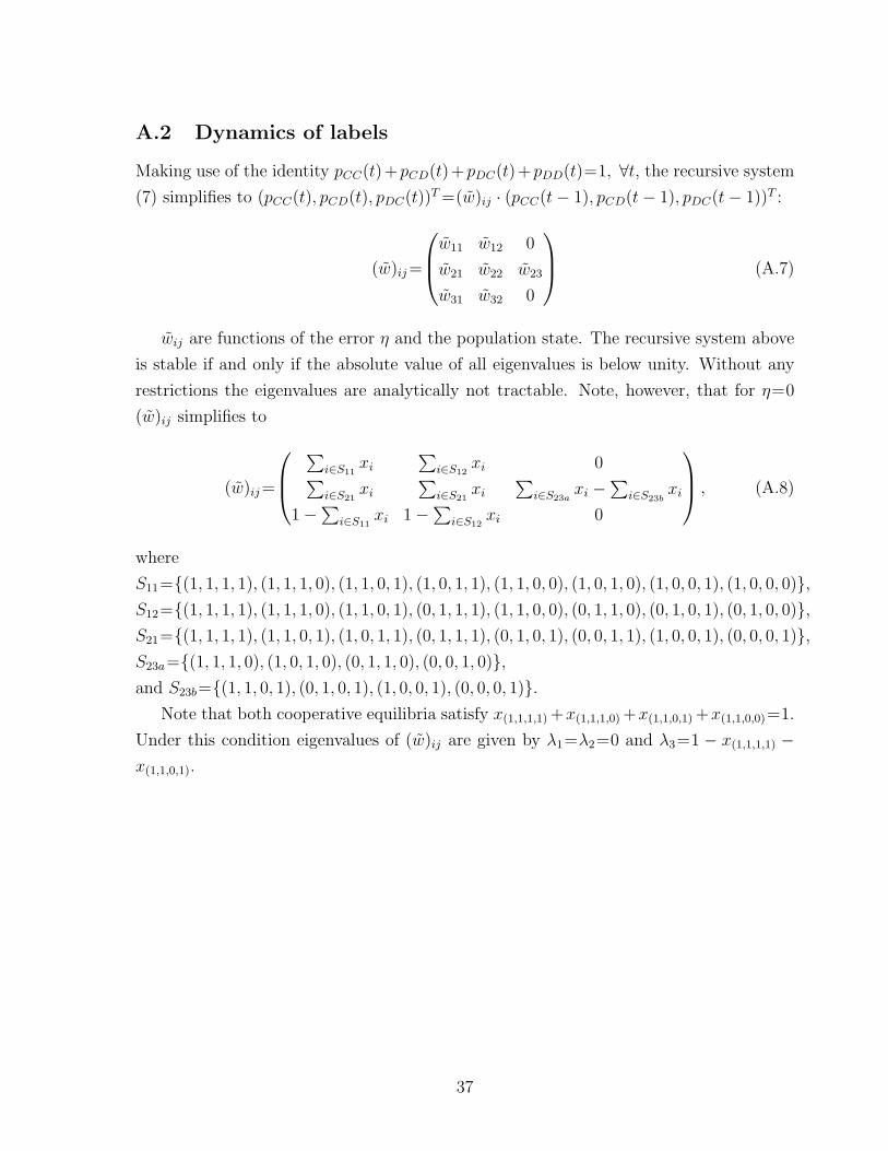
A.2 Dynamics of labels
Making use of the identity pCC(t)+pCD(t)+pDC(t)+pDD(t)=1, ∀t, the recursive system(7) simplifies to (pCC(t), pCD(t), pDC(t))
T=(w)ij · (pCC(t− 1), pCD(t− 1), pDC(t− 1))T :
(w)ij=
w11 w12 0
w21 w22 w23
w31 w32 0
(A.7)
wij are functions of the error η and the population state. The recursive system above
is stable if and only if the absolute value of all eigenvalues is below unity. Without any
restrictions the eigenvalues are analytically not tractable. Note, however, that for η=0
(w)ij simplifies to
(w)ij=
∑
i∈S11xi
∑
i∈S12xi 0
∑
i∈S21xi
∑
i∈S21xi
∑
i∈S23axi −
∑
i∈S23bxi
1−∑
i∈S11xi 1−
∑
i∈S12xi 0
, (A.8)
where
S11={(1, 1, 1, 1), (1, 1, 1, 0), (1, 1, 0, 1), (1, 0, 1, 1), (1, 1, 0, 0), (1, 0, 1, 0), (1, 0, 0, 1), (1, 0, 0, 0)},S12={(1, 1, 1, 1), (1, 1, 1, 0), (1, 1, 0, 1), (0, 1, 1, 1), (1, 1, 0, 0), (0, 1, 1, 0), (0, 1, 0, 1), (0, 1, 0, 0)},S21={(1, 1, 1, 1), (1, 1, 0, 1), (1, 0, 1, 1), (0, 1, 1, 1), (0, 1, 0, 1), (0, 0, 1, 1), (1, 0, 0, 1), (0, 0, 0, 1)},S23a={(1, 1, 1, 0), (1, 0, 1, 0), (0, 1, 1, 0), (0, 0, 1, 0)},and S23b={(1, 1, 0, 1), (0, 1, 0, 1), (1, 0, 0, 1), (0, 0, 0, 1)}.
Note that both cooperative equilibria satisfy x(1,1,1,1)+x(1,1,1,0)+x(1,1,0,1)+x(1,1,0,0)=1.
Under this condition eigenvalues of (w)ij are given by λ1=λ2=0 and λ3=1 − x(1,1,1,1) −x(1,1,0,1).
37

A.3 Distribution of labels over time, by treatment
Figure 4: Distribution of labels over time, by treatment.
A.4 Errors of implemenation
Period 4 vs. period 5 Period 10 vs. period 11 TotalLow cost treatment 4.8% (63) 9.0% (67) 6.9% (130)High cost treatment 5.5% (55) 10.7% (56) 8.1% (111)
Total 5.1% (118) 9.8% (123) 7.5% (241)
Table 6: Error rates, by treatment, in percentage (N in parenthensis).Error rates are the frequency with which a person stated C for a given label in period 5 or 10 did D for
that label in period 4 or 10.
A.5 Instructions
General instructions
1. Welcome and thank you for your participation! At the beginning of the experiment
you pulled out a cabin number and an envelope from a basket. PLEASE DO NOT
OPEN THE ENVELOPE! We will let you know when you can open the envelope.
This will happen only when the experiment is over and you have done ALL the
necessary tasks. If you violate this rule and open your envelope beforehand, we will
unfortunately be forced to exclude you from the experiment.
2. You can earn an amount of money in this experiment that depends on your choices
or those of another person. It is therefore very important that you read all the
38

instructions thoroughly and completely. Please switch off your mobile phones now!
Communication with other participants is not allowed. If you have a question, please
raise your hand. We will then come to you and answer your question.
3. In this experiment, as with all experiments in the Gottingen Laboratory of Behav-
ioral Economics (GLOBE), the participants shall not be deceived. If you are in any
doubt that the instructions correspond to the truth, then please contact lab@uni-
goettingen.de or a member of the Department of Microeconomics (Prof. Keser). All
data from this study is stored anonymously and kept strictly confidential.
4. Your earnings are calculated in ECU (Experimental Currency Units). 1 ECU equals
0.10e. At the end of today’s session, your total earnings will be converted into euros
and paid out confidentially and in cash. In addition, you will receive a participation
fee of 4e (40 ECU).
5. You and other participants are part of an experiment. This experiment goes on for
several periods. In each period you will be assigned to interact with another person
in today’s experiment. You will not meet that person a second time. You will never
know who the other people you meet are. The other people will not know your
identity.
6. In the experiment you are either a “decision-maker” or a “recipient”. The decision-
maker can choose between “keep” and “give.” If the decision-maker chooses “keep”,
the decision-maker receives 85 ECU and the recipient receives 40 ECU. If the
decision-maker chooses “give,” the decision-maker receives 75 ECU and the recipient
receives 65 ECU.
7. A paper in your envelope states whether you are the decider or the recipient. If
you are a decision-maker, the paper says “You are the decider.” The paper also
says which period will be relevant for payment. Every period can be relevant, but
only ONE period will actually be relevant for your payoff. Your decision in the
payoff-relevant period determines your payoff and the payoff of the person you met
in that period. If you are a recipient, the envelope says “You are a recipient.” Then
the decision of another person who was the decision-maker in the payoff-relevant
period will determine your payoff.
8. Every participant in this lab can be a decision-maker. Therefore, you should always
make your decisions as if you were a decision-maker and as if you were deciding
39

both your payoff and that of another person. You can not change your decision at
the end of the experiment. We will only implement the decision you made during
the experiment.
9. You are now asked to answer six control questions to check your understanding of
the instructions. The experiment will not begin until all participants have correctly
answered the control questions.
Control questions
1. Which period will be payoff-relevant? (The first period; Period 9; None; I do not
know that in advance. It’s in my envelope.)
2. Will your decisions be payoff-relevant or will decisions made by another person
determine your payoff? (My decisions will be payoff-relevant; The decisions of
another person will determine my payoff; I do not know that in advance. It’s in my
envelope.)
3. How many times will you meet the same person in this experiment? (Once; Every
period; I do not know that in advance.)
4. Will you know which person in the lab you meet in a given period? (Yes; No)
5. Will your identity be revealed to other people in the lab? (Yes; No)
6. Can the experimenters link your decisions with your name? (Yes; No)
Game instructions
1. The experiment begins now.
2. Periods 1 to 4 and 6 to 10 :
In period X, you meet someone new. You have two alternatives to choose from:
“keep” or “give.” If you choose “keep,” you will receive 85 ECU and the other
person will receive 40 ECU. If you choose “give”, you will receive 75 ECU and the
other person will receive 65 ECU.
[Period 2: The other person has chosen (give/keep) in the last period.
Period 3 to 4 and 6 to 10: The other person has chosen (give/keep) in the last
period, when faced with someone whom they knew had chosen (give/keep).]
Which alternative do you choose? (give/keep)
40

Info: In the next stage, you will be the recipient and another person will be the
decision-maker. This person will know which choice you have made.
[Period 2 to 4 and 6 to 10 : Info: In the next stage, you will be the recipient
and another person’s decision-maker. This person will know which choice you have
made. In addition, this person will learn what the person you have met this turn
had chosen before.]
3. Feedback: You have chosen (give/keep). The decision maker who meets you now
learns that you have chosen (give/keep).
[Period 2 to 4 and 6 to 10 : You have chosen (give/keep). The decision maker who
meets you now learns that you have chosen (give/keep) when faced with someone
who had chosen (give/keep).]
4. Control questions before period 3:
Suppose that one person has chosen (give/keep) when faced with someone whom
they knew had chosen (give/keep). Which of the following statements are true?
(a) Question 1: That person had chosen (give/keep) last period.
(b) Question 2: That person had chose (give/keep) two periods ago.
(c) Question 3: The person who was meeting that person had chosen (give /keep)
two periods ago.
5. Periods 5 and 11 :
In period X, we ask you about your decision plan for this period. We ask for your
decision when faced with someone you meet during this period. You will see various
possible information about the other person’s decision. For each case you have
to make a decision. Only at the end of the experiment, and if this period X is
relevant, will we give you information about the actual decision of the other person.
Your decision for the relevant case will then be executed and you will receive the
appropriate payoff. Please make sure that your decisions are in line with what you
want to see done at the end of the experiment!
You have two alternatives to choose from: “keep” or “give.” If you choose “keep,”
you will receive 85 ECU and the other person will receive 40 ECU. If you choose
“give,” you will receive 75 ECU and the other person will receive 65 ECU.
(The order of the following questions was randomized)
(a) Suppose that person chose to give in the last period, when faced with someone
41

they knew had chosen to give before. Which alternative would you choose in
this case?
(b) Suppose that person chose to give in the last period, when faced with someone
they knew had chosen to keep before. Which alternative would you choose in
this case?
(c) Suppose that person chose to keep in the last period, when faced with someone
they knew had chosen to give before. Which alternative would you choose in
this case?
(d) Suppose that person chose to keep in the last period, when faced with someone
they knew had chosen to keep before. Which alternative would you choose in
this case?
Payoffs
1. The game is now over. An experimenter will go through the lab to make sure none
of the envelopes have been opened. Please wait until we let you know that you can
open your envelope.
2. In your envelope is a paper telling you whether you are a decision-maker and which
period is relevant to your payoff. Please enter “Yes,” if your envelope states that
you are the decider. Please also enter the period that appears in your envelope.
The experimenter will come to you and will confirm your input so that you get to
the last part of the experiment.
3. Payoffs for the decision-maker:
You are a decision-maker. Your decision in period X determines your payoff and
the other person’s payoff.
Period 1: In period 1 you chose (give/keep). Period 2: In period 2 you chose
(give/keep). You knew that the other person had chosen (give/keep) in period 1.
Periods 3 to 11: In period X you chose (give/keep). You knew that the other
person had chosen (give/keep) in period X-1, when faced with someone you knew
had chosen (give /keep) in the previous period.
Therefore, you will receive XXX ECU and the other person will receive XXX ECU.
Converted into euros and with a participation fee of 4e, you will get XXX euros.
The other person will get XXX Euro.
42

4. Payoffs for the recipient:
You are a recipient. The decision of another person in period 1 determines your
payoff and the payoff of that person.
Period 1: In period 1 the other person has chosen (give/keep). Period 2: In
period 2 the other person has chosen (give/keep). This person knew that you had
chosen (give/keep) in period 1. Periods 3 to 11: In period X the other person
has chosen (give /keep). This person knew that you had chosen (give/keep) in
the period X-1, when faced with someone you knew had chosen (give/keep) in the
previous period.
Therefore, you will receive XXX ECU and the other person will receive XXX ECU.
Converted into euros and with a participation fee of 4e, you will get XXX euros.
The other person will get XXX Euro.
The payoff stage is now over. We still ask you to answer a number of survey questions,
after which you will be able to collect your remuneration.
Questionnaire
1. What do you think the experiment was about?
2. Please describe by which criteria you made decisions.
3. Do you think that the information provided to you was sufficient to make your
decisions? If not, what else would you have liked to know before you made your
decisions?
4. Was it hard for you to understand what you had to do in this experiment?
5. Did you have any difficulties during the experiment? If yes, please describe your
difficulties.
6. In how many experiments did you already participate in (approximately)? 1. I have
never participated in an experiment before. 2. 1-5 3. More than 5.
7. What kind of interactions did the experiment most likely remind you of? Inter-
actions with 1. family members. 2. friends. 3. classmates/work colleagues. 4.
strangers.
8. Do you know one or more of the other people who participated in today’s experi-
ment?
43

9. Do you think that you are similar to the other participants in today’s experiment?
10. Anna’s father has 5 daughters: Lala, Lele, Lili, Lolo, and .... What is the name of
the fifth daughter?
11. On a boat hangs a ladder with five rungs. The distance from one rung to the next
is 20cm. The lowest rung touches the water surface. The tide raises the water level
by 20cm per hour. How long does it take for the water level to reach the topmost
rung? 1. 5 hours. 2. 4 hours. 3. It never reaches it.
12. If it takes 20 minutes to boil a goose egg, how many minutes will it take to boil 3
geese eggs? 1. One hour. 2. 20 minutes.
13. Linda is 31 years old, single, very intelligent, and openly speaks her mind. She
studied philosophy. During her studies, she dealt extensively with issues of equal
rights and social justice and also took part in anti-nuclear demonstrations. Which
statement is most likely to apply to Linda? 1. Linda is a bank clerk. 2. Linda is a
bank clerk and is active in a feminist movement.
Finally, we would like to have some information about you.
1. How old are you? Please type in.
2. What is your gender?
3. What is your living situation? 1. I do not live alone. 2. I live alone.
4. Do you live in Gottingen?
5. Do you have German citizenship?
6. Are you worried about covering your living expenses over the next six months?
7. Do you think you are financially better off than others in your age group?
8. Are you currently enrolled for a degree?
9. Did you study economics in the past or are you now studying economics?
We thank you for your participation! You will now be called individually to receive your
payment. Please come to the experimenter in the entrance area when your cabin number
is called up. Please make sure you take all your belongings with you so you do not have
to go back to the cabin.
44