The Evolution of Descriptive and Substantive ...

The Evolution of Descriptive andSubstantive Representation, 1974–2004

David L. Epstein and Sharyn O’Halloran∗

1 Introduction

Following the 2000 census, Georgia redrew its 56 state senate districts so as to comply

with the one-person-one-vote rule. At the time, the Assembly and Senate both had

Democratic majorities. The governor, Roy Barnes, was a Democrat as well, and he

led the charge to construct a districting plan that would advantage his party in the

upcoming 2002 elections.

The key to this plan was to “unpack” many of the heavily-democratic districts

and distribute loyal democratic voters to surrounding districts. In particular, black

voters were reallocated away from districts with either especially high or low levels of

black voting age population (BVAP) in order to create more districts in the 25-40%

BVAP range, so-called “influence districts.” This meant that some districts with

black populations above 55% or 60% were brought down close to the 50% mark.

This strategy is illustrated graphically in Figure 1. To construct this graph, the

BVAPs in each district for both the pre-existing baseline plan and the proposed plan

∗Department of Political Science, Columbia University. Paper prepared for presentation at theConference on the 2007 Renewal of the Voting Rights Act, June 24-25, 2005. Preliminary Draft.Thanks go to the Russell Sage Foundation and the Carnegie Foundation for financial support.

1 INTRODUCTION 2

−.3

−.2

−.1

0.1

diff

0 20 40 60order

Proposed Plan vs. Baseline Plan

Changes in Black Voting Age Population

Figure 1: Is This Retrogression?

were sorted from highest to lowest, and the difference between corresponding entries

was calculated. The figure clearly shows the reallocation of black voters away from

the extremes of the distribution and towards the center.

The state submitted its plan directly to the DC District Court for preclearance,

and the Justice Department indicated its intention to interpose objections to Senate

districts 2, 12, and 26, whose BVAPs were slated to fall from 60.6% to 50.3%, 55.4%

to 50.7%, and 62.5% to 50.8%, respectively. The state submitted evidence showing

that the point of equal opportunity — the level of BVAP at which a minority-

preferred candidate has a 50% probability of winning — was 44.3%, and argued that

majority-minority districts should therefore give black candidates a healthy chance

1 INTRODUCTION 3

of gaining office. The DOJ disagreed, arguing that the state had not met its burden

of proving the proposed plan non-retrogressive.

The district court agreed with the DOJ and refused to preclear the plan. The

Supreme Court eventually overruled in the case Georgia v. Ashcroft,1 ruling that the

district court had not taken sufficiently into account the state’s avowed objective

of increasing substantive representation, even at a possible cost to descriptive

representation. The Court relied heavily on the testimony of black state legislators,

including civil rights leader and U.S. Representative John Lewis, who supported the

plan as an attempt to expand democratic control of state government.2

The reaction to Ashcroft was swift and heated. Karlan (2004) denounced the

decision as a first step towards “gutting” section 5 preclearance. Others claimed

that it “greatly weakened the enforcement provisions of Section 5.”3 An ACLU

official’s reaction was that “The danger . . . is that it may allow states to turn black

and other minority voters into second-class voters, who can influence the election of

white candidates but cannot elect candidates of their own race.” Others viewed the

decision more favorably: Henry Louis Gates wrote that “[Descriptive representation]

came at the cost of substantive representation — the likelihood that lawmakers,

taken as a whole, would represent the group’s substantive interests. Blacks were

winning battles but losing the war as conservative Republicans beat white moderate

Democrats.”4

Despite these conflicting overall assessments of the decision, a conventional

wisdom is forming on some key points of interpretation:

1539 U.S. 461 (2003).2The plan passed with the concurrence of 44 out of 45 black state legislators.3Benson (2004).4New York Times, September 23, 2004.

1 INTRODUCTION 4

1. In Ashcroft, the Court abandoned a previous, “relatively mechanical” retro-

gression test based on electability;

2. It did so in favor of an amorphous concept of substantive representation that

will be difficult to administer; and

3. The crux of the debate revolves around the tradeoffs between substantive and

descriptive representation.

In this essay we take issue with all three of these propositions. First, we argue,

along with Pildes (2002), that tests for retrogression based on issues of descriptive

representation alone were becoming increasingly harder to maintain in light of

changed political conditions, including increased white crossover voting and the rise

of the republican party in the south. In fact, one of the less-discussed features of

Ashcroft is that it replaced the previous, district-by-district approach to assessing

retrogression in descriptive representation with a statewide approach, in which losses

in one part of the state could be offset by gains elsewhere.

Second, we argue that substantive representation need not be viewed as “fuzzy”

or difficult to measure. Consistent with our previous work5 and recent advances in

the statistical analysis of roll call data,6 we define a members’ minority support score

as the degree of concordance between that member’s voting record and the voting

records of minority legislators. This measure can be calculated to prospectively assess

the likely impact of competing redistricting plans, or to compare a given plan to the

status quo baseline.

Third, we do not accept that these debates are all, or even mostly, about having

to decide between descriptive and substantive representation. Most advocates of

5Cameron, Epstein and O’Halloran (1996), Epstein and O’Halloran (1999a; 1999b).6Poole (2005).

2 ASHCROFT AND RETROGRESSION 5

restricting section 5 review to electability issues alone — that is, the critics of Ashcroft

— do so not just because they value descriptive representation per se, but because

they believe that the election of minority representatives is the surest, least risky

way to ensure minority voters of substantive representation.7 If we are correct, then

the points of disagreement are more quantifiable than much of the previous debate

would suggest.

This essay first locates the Ashcroft decision within the broader discussion of

race, redistricting and representation as it has evolved in the legal and social science

literatures in the past four decades. Second, we document the emerging tradeoff

between substantive and descriptive representation for both black and Hispanic

voters, for the years 1974 to 2004. The data indicate that up until roughly the mid-

1980s districting schemes that maximize descriptive representation were identical to

those that maximized substantive representation. Over the past decade-and-a-half,

though, these two objectives diverged. We also investigate the interrelations between

the numbers of black and latino voters in a district and the consequent probabilities

of electing one or the other type of candidate to office.

2 Ashcroft and Retrogression

The starting point for section 5 preclearance is, of course, retrogression. Ever since

Beer,8 retrogression has been the standard for discriminatory effect, and since Bossier

II,9 it is the standard for discriminatory purpose as well. But the exact meaning of

“retrogression” in the context of redistricting has always been a bit unclear. After

all, voters excluded from one district do not simply disappear; they are reallocated

7There are also significant partisan issues in this debate, but we do not treat these questionshere.

8Beer v. United States, 425 U.S. 130 141 (1976).9Reno v. Bossier Parish School Board, 528 U.S. 320 (1999).


to surrounding districts, where they have the potential to influence the selection of

a different representative.

Let us leave aside for the moment the complicating issue of substantive

representation and focus on the steps for determining whether a districting plan is

retrogressive on grounds of descriptive representation alone. Three steps are required:

1) calculating the difference between the proposed and baseline plans; 2) translating

this difference into a statement about electability pre- and post-redistricting; and 3)

translating this determination of electability into a conclusion about retrogression.

This section argues, first, that even before Ashcroft the Justice Department’s

criteria for assessing retrogression were becoming less and less coherent, given the

significant changes that had been taking place in the electoral environment. We

next discuss the Ashcroft ruling in relation to this traditional, electability-based

standard. Finally, we argue that Ashcroft requires new measures of both descriptive

and substantive representation for consistent implementation.

2.1 Pre-Ashcroft Preclearance

Let us begin by dissecting the body of argumentation surrounding the Justice

Department’s pre-Ashcroft criteria for approving a redistricting plan. Up until

now, the DOJ has interpreted retrogression with respect to issues of descriptive

representation alone:

A proposed plan is retrogressive under the Section 5 “effect prong” if its

net effect would be to reduce minority voters’ “effective exercise of the

electoral franchise” when compared to the benchmark plan. The effective

exercise of the electoral franchise usually is assessed in redistricting

submissions in terms of the opportunity for minority voters to elect


candidates of their choice.10

This approach implies that one compares baseline and proposed plans by counting

the number of districts with BVAPs11 above some crucial threshold necessary for

minority voters to have effective control over elections.12 This also serves as a

proxy for changes in electability, and retrogression is established if this number

decreases. The answers to the three questions posed above are therefore relatively

straightforward under this approach.

Several hidden assumptions, however, are required to justify this method. First,

the comparison between the baseline and proposed plans works on a district-by-

district basis. Consequently, one must be able to establish a correspondence between

the proposed and pre-existing districts. Since redistricting could potentially draw

lines in any manner that results in equally populated divisions, this one-to-one

correspondence maybe problematic.

Second, equating electability with the number of districts over some threshold

works best if minority-supported candidates have very little chance of winning under

that threshold, and near certainty of winning above it. This would be the case, for

instance, if voting is highly polarized with little crossover between white voters and

10Guidance Concerning Redistricting and Retrogression under Section 5 of the Voting Rights Act,Federal Register, January 18, 2001, at 5411-5414 (hereafter referenced as “Guidance ConcerningRedistricting”). This is consistent with the Court’s declaration in Bush v. Vera that non-retrogression “mandates that the minority’s opportunity to elect representatives of its choice notbe diminished, directly or indirectly, by the State’s actions.” (517 U.S. 952, 983 (1996).

11For ease of discussion, we will refer mainly to BVAPs and black voters in the following sections.It should be understood that these arguments apply equally to hispanics or any other communityof interests under the VRA.

12These thresholds are often summarized as a single percentage of minority residents. At first,the rule of thumb was 65% total black population. More recently, the informal standard hasbeen 50% BVAP, termed “majority-minority”. The DOJ has consistently maintained that itscriteria for assessing electability are much more nuanced than any single-number approach. SeeGuidance Concerning Redistricting : “Although comparison of the census population of districts inthe benchmark and proposed plans is the important starting point of any retrogression analysis, ourreview and analysis will be greatly facilitated by inclusion of additional demographic and electiondata in the submission.”


minority candidates, and vice-versa. It thus admits of no grey areas or tradeoffs

across districts, for instance by shifting minority voters in such a way as to decrease

the probability of electing a minority candidate from 85% to 75% in district x, but

raising the probability from 35% to 50% in district y. But when the probability

of minorities gaining office rises gradually with changing district composition, these

sorts of tradeoffs become more real, and the single-threshold approach becomes more

arbitrary.

This state affairs is illustrated with sample data in Figure 2, which graphs the

probability of electing a minority-supported representative as a function of percent

black voting age population. The key threshold as drawn in the figure is 57.5%

BVAP: below this point minorities have almost no chance of controlling an election

while above it they are nearly assured of such control. Note that 57.5% BVAP also

serves as the “point of equal opportunity”; the point at which minority candidates

have an even chance of winning an election. Thus equal opportunity, electability,

and minority control coincide perfectly in this world.

2.2 A Menagerie of Districts

The contrasting case is illustrated in Figure 3. Here the probability of electing

minority candidates rises more slowly, so that gradual increases in BVAP produce

gradual, rather than abrupt, changes in electoral probability. It also admits of the

possibility that the point of equal opportunity could fall below 50% BVAP: in the

figure, it occurs at 40%.

This complicates the electability calculus enormously. Figure 4 illustrates the

key cut points in worlds with high and low polarization, respectively. In the high

polarization example, the point of equal opportunity, labeled P ∗, divides districts


0.5

1P

rob

ab

ility

of

Ele

ctin

g B

lack R

ep

.

0 50 57.5 100Percent Black Voting Age Population

Figure 2: Probability of Election vs. BVAP with High Electoral Polarization

with and without minority control. As long as P ∗—which was 57.5% in Figure

2—remains above 50%, there is no conflict between electability and control.

The lower half of the figure, though, illustrates a situation when P ∗ slips below

50%. For districts with BVAPS under P ∗, minority control is less likely, although if

the situation illustrated in Figure 3 holds, electability will not drop off dramatically.

This creates a range of districts between P ∗ and 50% which Pildes (2002) terms

“coalitional districts.” Here, it is relatively likely that minority-supported candidates

will be elected, but they must rely on white crossover voting to do so. In this case, it

might be argued, minority voters lack the degree of control they had with majority-

minority districts, since their preferred candidate may have to accommodate the


0.5

1P

rob

ab

ility

of

Ele

ctin

g B

lack R

ep

.

0 40 50 100Percent Black Voting Age Population

Figure 3: Probability of Election vs. BVAP with Low Electoral Polarization

% BVAP0

P*

50 100

No Minority Control

HighPolarization

Measuring Descriptive Representation

Minority Control

% BVAP0

P*

50 100

No Minority Control

SafeControl

PS PP

Coali-tional

UnsafeControl

Packing

LowPolarization

PI

Influence

Figure 4: Key Points and District Types


preferences of non-minority voters to gain office.

The situation becomes even more complicated by the Justice Department’s

introduction of “safe minority districts” in Ashcroft. Although they never define

this term precisely, it would seem to indicate a point at which the probability of

minority candidate’s attaining office is considerably greater than 50%. In particular,

they argue that the redistricting plan for the Georgia State Senate at issue in Ashcroft

was retrogressive because it reduced the number of these safe districts. And since

the three districts that they objected to all had BVAPs just above 50%, we can

assume that the “safety point”, labeled P S in the figure, is considerably above the

50% mark.13 Note that this introduces two more district categories: those between

50% and the safety point, and those above the safety point. In the figure we term

the former the region of “unsafe minority control”, and the latter the region of “safe

control.”

We also include the point P I to indicate the boundary of influence districts, those

districts in which “a minority group has enough political heft to exert influence on

the choice of candidate though not enough to determine that choice.”14 We define

this boundary more precisely as the point of “democratic equal opportunity:” the

level of BVAP at which a democratic candidate has an equal chance of winning the

election.15

A final division is suggested by the DOJ’s statement in Guidance Concerning

Redistricting that they will reject plans in which “minorities are over-concentrated

13Pildes (2002), written prior to the DOJ’s objections to Georgia’s proposed plan, conflates thecategories of majority-minority and safe districts. The DOJ clearly considers them to be distinct.

14Barnett v. City of Chicago, 141 F.3d 699, 703 (7th Cir. 1998) (opinion by Posner, J.), cert.denied (1998).

15This is consistent with Karlan’s (2004) definition of influence districts as those in which “whitecandidates defeat black preferred candidates in the democratic primary but in which the democraticcandidate wins the general election.”


in one or more jurisdictions;” that is, packing. The point over which districts are

packed is labeled P P in the figure, bringing the total number of possible district

types up to six.

Such a menagerie of choices immediately raises difficult questions about tradeoffs.

How many conational districts does one need to outweigh one safely controlled

district? Or perhaps some combination of coalitional and unsafe districts may

outweigh one safe district? Or perhaps, as the DOJ argued, there is no combination

of other district types that could possibly offset the loss of even one safe district.

The latter position implies a “ratchet effect” in safe districts: their number can be

increased from one decade to the next, but never decreased.

Last, electability is a good proxy for retrogression only if it correlates highly

with other types of representation. In particular, descriptive representation will go

hand-in-hand with substantive representation in a world where legislators will fight

for minority-supported policies if and only if they were elected in contests controlled

by minority voters. That is, it rests on the assumption that legislative voting is as

polarized as voting in the electorate. Analogous to the example above, we would not

have to worry about reducing substantive minority support 10% in one district in

order to increase it by 20% in another.

In this situation, one would give minimal credence to the efficacy of influence

districts, since minority electoral control is the key to substantive representation.

This avoids sticky questions of how many influence districts it would take to outweigh

one minority-controlled district, similar to the tradeoffs considered above. Of course,

if the exclusive focus of retrogression analysis is on electability, such concerns fade

to the background anyway.

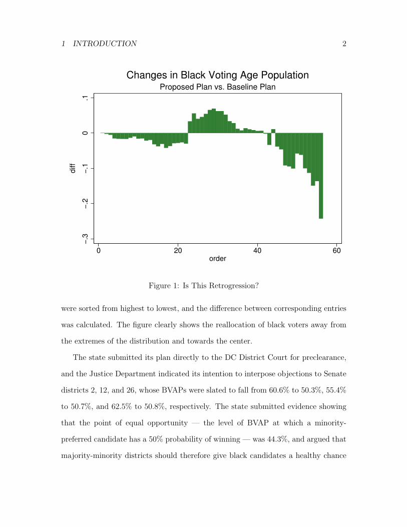
As we will show below, the assumptions of polarized voting both in the public


Substantive

Descriptive

SQ

1

2 3

4 P

ParetoFrontier

Retrogression Before and After Georgia v. Ashcroft

•Pre-Ashcroft: Areas 2 and 3 were permissible proposal P is retrogressive•Post-Ashcroft: Areas 2, 3, and 4 are permissible P is non-retrogressive

Figure 5: Pareto Frontier of Descriptive and Substantive Representation

and in Congress were a fairly accurate description of reality in the South up until

sometime in the 1980s. Since then, though, the world has become much more

complicated, so that the Justice Department’s algorithm for assessing redistricting

submissions may now be called into question.

2.3 Life on the (Pareto) Frontier

To frame our argument concerning substantive and descriptive representation,

Figure 5 shows a two-dimensional graph, with substantive representation on the

horizontal axis and descriptive representation on the vertical axis.

Assuming for the moment that a tradeoff between these two objectives does in

fact exist, there will be a “Pareto frontier,” a term borrowed from economics to


describe the maximum possible combination of each type of representation. Starting

from any point on the frontier, there is no other achievable point that is better in

one dimension and at least as good in the other. Conversely, any increase in one

quantity necessarily requires a decrease in the other.

There are, of course, points inside the frontier, one of which is labeled “SQ” in

the figure, indicating that it is the baseline, or status quo, state of affairs. The

lines drawn through SQ divide the Pareto region into four quadrants. Moves from

SQ to Region 3 improve both substantive and descriptive representation and are

termed Pareto improving. Conversely, movements into quadrant 1 are worse in each

dimension. And regions 2 and 4 represent improvements in one dimension at the

costs of decreases in the other. For example, the point labeled P in the figure,

representing a proposed change from the status quo to region 4, would increase

substantive representation at the cost of descriptive representation.

It is tempting to conclude that jurisdictions should be required to move to

the Pareto frontier whenever possible, but we reject such a strong interpretation

of the diagram. First of all, the exact districting schemes needed to move to

the frontier could be very difficult to devise, and they may well violate other

standard redistricting criteria such as compactness and regard for preexisting political

subdivisions. Second, while theoretically attractive, there may be some points on

the Pareto frontier that may be regarded as normatively suspect. The point that

maximizes descriptive representation, for example, might give minority voters a share

of legislative seats greater than their population proportion.16 Similarly, the point

that maximizes substantive representation might well result in electing no minorities

at all to office; this outcome would undoubtedly represent a major step backwards

16In first-past-the-post elections, a minority group which constitutes x percent of the populationcould theoretically control up to 2x percent of the legislature.


in minority voting rights, whatever positive policy implications it might have.

Note that when voting in both the electorate and legislatures is polarized,

increases (and decreases) in substantive and descriptive representation go hand-in-

hand. With reference to the figure this would translate into the statement that

regions 2 and 4 do not exist and the only possible moves are into regions 1 and

3. But the major thesis of this paper is that these tradeoffs do now exist; in fact,

the redistricting plan passed by the Georgia State Legislature was, in expectation, a

move into region 4.

How do these regions translate into decision rules regarding retrogression and

preclearance? In a regime where retrogression is measured by changes in descriptive

representation alone, the only question is whether the proposed plan lies above or

below the status quo on the vertical axis. Moves from SQ to regions 2 or 3, that is,

would be permissible, while moves to regions 1 and 4 would be retrogressive.

Ashcroft, however, declared that legislatures can enact plans which they expect

to increase substantive representation, even at a possible small cost to descriptive

representation. In our framework, the Ashcroft decision can be simply summarized

as allowing moves to region 4 as well as regions 2 and 3, leaving only the Pareto

inferior moves to region 1 as retrogressive.

It is important to immediately circumscribe this interpretation of Ashcroft. First,

the plan enacted by the Georgia state legislature received strong support from the

minority representatives, and, as noted above, the Court gave significant weight to

this fact in its decision. A similar plan passed, for instance, by a Republican majority

over the objections of black legislators would probably not receive such a favorable

evaluation. Second, the Court did not attempt to set limits on the scope of such

moves, and it would probably not look favorably on changes like those noted above

3 MEASURING DESCRIPTIVE AND SUBSTANTIVE REPRESENTATION 16

which would significantly increase substantive representation but deny any minority

legislators a reasonable chance to win office. Ashcroft should simply be read as

announcing that region 4 is not ex ante out of consideration when mapping out a

redistricting plan.

In taking this view of the Ashcroft decision we therefore part ways with Issacharoff

(2004), who claims that the Court “substituted a highly nuanced totality-of-the-

circumstances approach for the relatively rigid Beer retrogression test.” To the

contrary, we view Ashcroft as simply extending the set of criteria that can be applied

to determine retrogression. This assumes that substantive representation can be

measured in at least as objective a fashion as descriptive representation, the topic to

which we now turn.

3 Measuring Descriptive and Substantive Representation

Justice’s Souter’s dissent in Ashcroft sharply questions the administrability of the

majority decision, declaring it “simply not functional in the political and judicial

worlds.”17 A number of observers echo these concerns, implying that the Ashcroft

Court abandoned an easily-applicable retrogression test based on electability in favor

of recognizing the amorphous concept of substantive representation. Issacharoff

(2004), for example, claims that previous Supreme Court decisions had

narrowed section 5 to questions that could be addressed through relatively

mechanical assessments of voting practices. For example, the Beer

retrogression test made it easy to decide that a districting arrangement

in a town with a twenty-percent black population that yielded one forty-

five-percent black district (out of five) should not be precleared if the

17Id. at xxx.


prior arrangement had afforded one district that was sixty-five-percent

black.18

We agree that Ashcroft would be meaningless, or worse, without consistent,

administrable measures of substantive representation. But we also emphasize that

those who claim Ashcroft abandoned a previous set of clear, electability-based

standards for preclearance do not understand the full force of Pildes (2002). Even

had the court kept preclearance within the ambit of descriptive representation alone,

it would nonetheless have had to create new standards. We first review these issues,

then turn to our proposed measure of substantive representation and combine them

into an overall index that can be used to compare competing redistricting plans.

3.1 Defining Descriptive Representation

The central point of Pildes (2002) was to emphasize that the election of minority-

preferred representatives has ceased to be, so to speak, a black-white issue. There is

no longer a magic number above which a minority can control the electoral outcomes

of a district and below which they do not: electability is now a matter of degree.

Those who express the view that the Beer retrogression test would have been easy to

implement in this new environment of decreased electoral polarization and increased

crossover voting are, we argue, looking for the on-off switch in a room where all the

lights are on dimmers.

Let us assume the contrary; that there is a straightforward way to test for

electability-based retrogression when comparing a proposed plan to its baseline. In

decreasing order of strictness, we can imagine the following list of possibilities:

1. A state cannot decrease the BVAP in any district that currently has greater

18Karlan (2004) expresses similar concerns.


than 50% BVAP;

2. A state cannot decrease the BVAP in any district that currently elects a

minority-preferred candidate to office;

3. A state cannot reduce the number of districts below a “safe” level of BVAP;

4. A state cannot reduce the number of districts with greater than 50% BVAP;

5. A state cannot reduce the number of districts with BVAP greater than the

point of equal opportunity.

Other rules can clearly be added as well. The point is that a marginal change in a

district’s composition now results in a marginal change in the probability of electing

a minority-preferred candidate. One essential task of laws is often, of course, to

draw bright lines that divide continuous outcomes. But none of Ashcroft ’s critics

have indicated where they would draw such a line, and given the fact that the point

of equal opportunity is now under 50% BVAP, as Pildes (2002) argues, no natural

dividing line presents itself.

Indeed, one aspect of the Ashcroft decision that has sofar gone unnoticed, is that

it abandoned the previous district-by-district method of comparing two districting

plans in favor of a method that explicitly allows for tradeoffs across districts:

First, while the District Court acknowledged the importance of assessing

the statewide plan as a whole, the court focused too narrowly on proposed

Senate Districts 2, 12, and 26. It did not examine the increases in the

black voting age population that occurred in many of the other districts.

Second, the District Court did not explore in any meaningful depth


any other factor beyond the comparative ability of black voters in the

majority-minority districts to elect a candidate of their choice.

Notice that the opinion chides the district court for failing to take tradeoffs into

account before it adds that they should consider issues of substantive representation

as well. The implication is that, even were substantive representation not an issue,

a determination of retrogression should allow for increases in one district to be able

to offset loses in another.

The cleanest way to escape the menagerie of district types, and to allow for the

inter-district tradeoffs that the Supreme Court now mandates, is to simply estimate

the probability that each district in a given redistricting plan will elect a minority

candidate to office. Given the past history of elections in the relevant jurisdiction,

curves like those drawn in Figures 2 and 3 can be estimated using standard statistical

techniques.19 Two plans can then be compared according to both the average

(expected) number of minority-preferred candidates elected to office, and by the

variance around this number.

To compare two plans, one need not be forced to accept the proposition, as

Karlan (2004) implies, that a 50-50 chance of winning 20 districts is just as good as

a certainty of winning 10; there may be valid reasons for favoring continued success

of a limited number of candidates, such as the accrual of seniority, experience and

name recognition. Formally, such considerations could be included in the analysis as

risk aversion, preferring certain to risky outcomes. But unless one begins with the

full set of election probabilities, retrogression determinations will be driven by a set

19The logit and probit models are the two most commonly used estimators for qualitativedependent variables. Probit analysis, for instance, was used to estimate the 44.3% point ofequal opportunity in Ashcroft. See Epstein and O’Halloran (1999b) for analysis of the statisticaladvantages of probit estimation over ecological regression.


of increasingly arbitrary categories and definitions.

3.2 Defining Substantive Representation

Which brings us to the question of how to define substantive representation. We

propose here to use the same measure developed in our previous essays:20 namely,

the percent of times that a given legislator votes in concert with the majority of the

minority representatives, which we term a member’s Minority Support Score.

Social scientists have developed sophisticated methodologies in the past decade

for inferring legislative preferences from their roll call voting patterns,21 and these

measures have subsequently been used in dozens of essays in leading journals.

These measures are used not because they are assumed to capture the totality of

legislators’ actions; after all, constituency service, committee work and behind-the-

scenes maneuvering are at least as important as final roll call votes. Rather roll call

voting behavior has been shown to be highly correlated with these others measures

of representation in various contexts, making it an appropriate summary measure of

substantive representation.

The object of this analysis, then, is to estimate the relation between a district’s

composition and representative characteristics on the one hand, and roll call voting

behavior on the other. Notice that this is consistent with the view of representation

implicit in previous discussions of the Voting Rights Act and section 5 preclearance:

candidates of choice are important not for their race or ethnicity,22 But because they

will represent the minority group’s concerns in the legislature.

This relationship also lies at the heart of discussions of coalitional and influence

20Cameron, Epstein and O’Halloran (1996); Epstein and O’Halloran (1999).21See Poole and Rosenthal (1985); Jackman and Treier (2003); and Poole (2005).22Gingles made it clear that “It is the status of the candidate as the chosen representative of a

particular racial group, not the race of the candidate, that is important.”


districts, although not always in a consistent manner. Worries about coalitional

districts, for instance, can be based on a median voter theory of representation. If

the voter at the 50th percentile of the distribution is non-minority, that is, then

the representative will be forced by electoral concerns to move her policies in a

more conservative direction, thus reducing minority influence. Once understood in

this light, concerns about coalition districts become understandable on substantive

rather than descriptive representation grounds.23

Influence districts are based on the somewhat contradictory notion that represen-

tatives who rely on a large block of voters for reelection must take their concerns into

consideration once in the legislature. Under an median voter argument, of course,

this is not the case: black voters are unlikely to cast their ballots for republican

candidates anyway, and so representatives will aim their policy positions are the

center of the preference distribution. Small groups in a district may have significant

influence, though, if politics consists of more than a single left-right continuum.

There may be particular issues that a small group cares deeply about but are less

important to the majority. If minority voters can organize themselves and lobby their

representatives on this discrete set of issues, they may wield considerable influence

in these issue domains.

In the end, there is no general consensus within political science as to which model

of representation dominates; different models are often appropriate for different

issue areas. For our concern here, the question is an empirical one: given a

representative’s party and race, does the addition or subtraction of minority voters

from a district impact her voting behavior? Or, to the contrary, are levels of

23For these concerns to be valid, one must assume that minority voters are homogeneous anduniformly more liberal than any of the non-minority voters in the district. To the degree that thereis some mixing of preferences at the liberal end of the scale, such concerns become less pressing.


substantive representation a fairly constant within groups of representatives sharing

similar partisan and racial characteristics, regardless of their district BVAP?

3.3 Implementing Ashcroft

It is now straightforward to combine these measures of descriptive and substantive

representation to produce the expected level of substantive representation. For any

given level of BVAP, we can estimate the probability that a republican, white

democrat or black democrat will be elected and, for each of these types, we

can estimate their expected level of support for minority-supported issues. The

overall expected level of substantive representation is then the product of these two

quantities.

Assume for example that a 40% BVAP district has a 10% chance of electing a

republican, 50% chance of electing a white democrat, and a 40% chance of electing a

black democrat. Further assume that a republican elected from a 40% black district is

expected to have a black support score of 40, a white democrat from such a district

is expected to have a support score of 90, and a black democrat has an expected

support score of 100. Then the overall expected support from such a district is

(0.1 ∗ 40) + (0.5 ∗ 90) + (0.4 ∗ 100) = 89. For a districting plan, one adds up these

numbers district-by-district to obtain the total substantive representation, and these

summary statistics can be compared across plans.

As with descriptive representation, one is free to include the uncertainty in these

outcomes as part of the decision process. A plan with a guaranteed average score of

80 might well be preferred to a plan with a 50% chance of 60 and a 50% chance of 100.

The point is not to argue that states must choose the plan with the higher average

support score even if it comes at the cost of higher variance; covered jurisdictions


may exhibit risk aversion just as readily as do consumers and investors.

One might wish to add other considerations to this calculus, including, for

instance, the probability that one party or another controls a majority of the

legislature. Such considerations, though, would violate our reading of the “black box”

approach to section 5 preclearance implied by Presley v. Etowah County24. Under

Presley, actions taken inside the legislature do not fall under section 5 preclearance,

and the organizing role played by majority parties would fall into this category.25

It is our contention that this measure of expected substantive representation is in

fact identical to the mental model being used by advocates of safe minority districts.

They, too, imagine a world where each legislator is assigned a number between 0 and

100, indicating the degree to which they will work to pursue minority policy goals.

It is just, we contend, that these advocates believe that the only numbers which will

appear in practice are either 0 or 100 (or there about), and that the only way to

assure oneself of a high-type representative is to ensure that minorities control the

electoral process.

Even presented with evidence that non-minority representatives can have fairly

high support scores, they might counter that a) such scores are not a true

measure of their degree of support, since there are many other behind-the-scenes

services performed by candidates of choice but not by these “impostors,” including

constituency relations and working to put important minority issues on the legislative

agenda; and/or b) that these intermediary-type representatives do not provide secure

representation—as Karlan (2004) notes, they may switch parties or abandon the

minority voters who helped them get elected in the first place—so it would be folly

24502 U.S. 491 (1992).25As noted by Karlan (2004) the Court’s reference in Ashcroft to the value of maintaining

committee chairmanships comes dangerously close to transgressing into the legislative sphere andaway from a minority groups’ right to cast and effective vote.

4 THE EMERGING TRADEOFF 24

to let go of two or three birds in the hand for the prospect of six or even eight fly-

by-night birds in the bush. They advise states to heed the first rule of wing-walking:

Don’t let go of what you’ve got hold of, until you have hold of something else.

These are all valid concerns, but they do have their limits. If risk aversion is

so high that no compromises of descriptive representation are ever allowed, then

the system will literally never change to one based more on coalition building and

fluid bargaining. We view possible tradeoffs between descriptive and substantive

representation, and the risks inherent in moving from one to the other, as the epitome

of political choices, rightfully made by voters through their elected representatives,

and not to be imposed from above by a possibly over-weaning federal administration.

4 The Emerging Tradeoff

We now explore patterns in electoral and legislative politics over the past 30

years, examining the evolution of descriptive and substantive representation of

black and Hispanic voters. For both groups, the trends over time have been for

voting in the public to become less polarized, while voting in Congress becomes

more polarized. As a result, the districting strategies that maximize substantive

and descriptive representation in the south now diverge, and we present evidence

graphically displaying the resulting Pareto frontier.

4.1 Black Representation

We analyze data from the House of Representatives between 1974 and 2004.26 For

each election held during that period, we recorded the party and race (white,

black, Hispanic) of the winning candidate. We also calculated the black voting

26Data from the 2001-2004 period will be incorporated in future drafts.


age population (BVAP) and Hispanic voting age population (HVAP) of the district,

interpolating between census estimates to impute district demographics. In addition,

we coded the region in which the election took place: east, south, or west.27

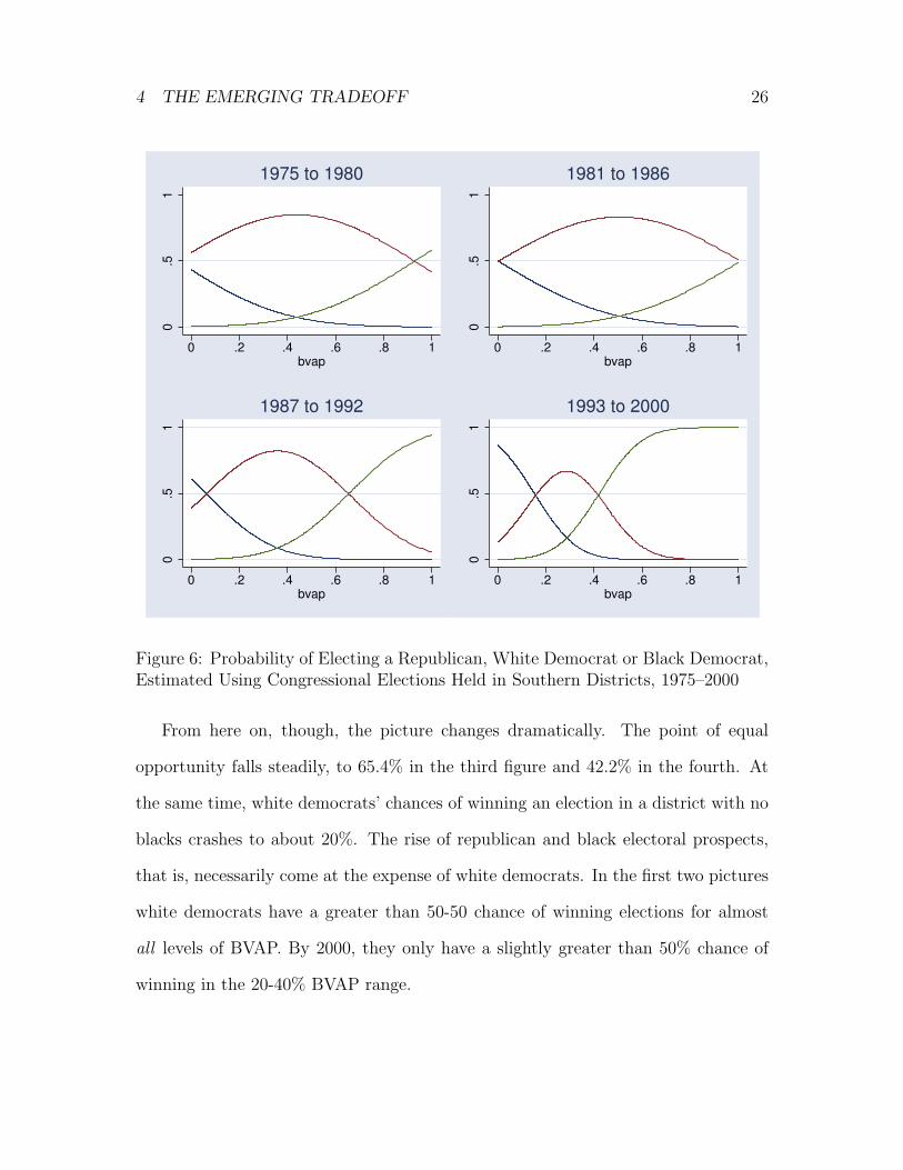
4.1.1 Descriptive

For the analysis of black electoral opportunity, we divided representatives into three

types: republicans, white democrats and black democrats. We then performed an

ordered probit analysis on this representative type using BVAP as an independent

variable for each congress and region. The results of this analysis, grouped into

four time periods, are shown in graphical form for southern districts in Figure 6. In

each graph, the central curve represents the probability of electing a white democrat,

the curve reaching its maximum at low levels of BVAP indicates the probability of

electing a republican, and the line reaching its maximum at high levels of BVAP is

the probability of electing a black democrat. These graphs also include a horizontal

line at 0.5; the level of BVAP where this line intersects the black democrat curve

indicates the “point of equal opportunity;” the level of BVAP needed to give a black

democrat a 50-50 chance of winning election.

As shown in the figure, from the mid-1970’s to the mid-1980’s, white democrats

were still the dominant group in southern politics. In fact, the point of equal

opportunity is estimated at over 100% in the 1981–1986 period, since a number

of southern districts with majority black populations still elected white democrats

(such as Hale and then Lindy Boggs from Louisiana). And even in an all-white

district (0% BVAP), republicans have no better than an even chance of winning.

27Southern states are Alabama, Arkansas, Florida, Georgia, Kentucky, Louisiana, Mississippi,North Carolina, Oklahoma, South Carolina, Tennessee, Texas, and Virginia. Eastern states areConnecticut, Delaware, Maine, Maryland, Massachusetts, New Hampshire, New Jersey, New York,Pennsylvania, Rhode Island, Vermont, and West Virginia. “West” indicates all other states.


0.5

1

0 .2 .4 .6 .8 1bvap

1975 to 1980

0.5

1

0 .2 .4 .6 .8 1bvap

1981 to 19860

.51

0 .2 .4 .6 .8 1bvap

1987 to 1992

0.5

1

0 .2 .4 .6 .8 1bvap

1993 to 2000

Figure 6: Probability of Electing a Republican, White Democrat or Black Democrat,Estimated Using Congressional Elections Held in Southern Districts, 1975–2000

From here on, though, the picture changes dramatically. The point of equal

opportunity falls steadily, to 65.4% in the third figure and 42.2% in the fourth. At

the same time, white democrats’ chances of winning an election in a district with no

blacks crashes to about 20%. The rise of republican and black electoral prospects,

that is, necessarily come at the expense of white democrats. In the first two pictures

white democrats have a greater than 50-50 chance of winning elections for almost

all levels of BVAP. By 2000, they only have a slightly greater than 50% chance of

winning in the 20-40% BVAP range.


4.1.2 Substantive

For our measure of substantive representation we started with all Congressional

Quarterly key votes taken during this period. For each roll call we tabulated the Aye

and Nay votes, coding all abstentions, absences and pairs as missing data. We then

determined which position was taken by the majority of the black representatives

who cast a valid vote and coded that as a vote in the pro-minority direction. Finally,

we calculated the black support score for each member and each congress as the

percent of times that member voted with the black majority.28

Support scores as a function of the district black voting age population are

shown for southern representatives for each of the four time periods in Figure 7.

The relation between BVAP and support has been estimated using a fractional

polynomial fit, which is a standard method for summarizing a possibly non-linear

relationship between two variables.29 In each graph, the uppermost line represents

black democrats, the next down is white democrats, and the bottom is republicans.

As shown in the figure, the support scores are relatively constant within each

representative type; the major source of variation is found across types. White

democrats at higher levels of BVAP do seem to become more liberal in the second

and third groups, but then they reverse this trend a bit in the fourth. However, in

all cases 95% confidence bands show that the null hypothesis of a constant function

within each group cannot be rejected, so these apparent trends may be due merely

to chance.

The republicans and black democrats have fairly similar support scores in all

periods; the biggest change comes from white democrats, whose average support

28We also calculated support scores taking into account the degree of unanimity among the blackrepresentatives; this variant had only a minimal impact on our final results.

29The lines in the graphs were generated using Stata’s fpfit command.


.2.4

.6.8

1B

lack S

upport

Score

0 .1 .2 .3 .4Black Voting Age Population

1975 to 1980

.2.4

.6.8

1B

lack S

upport

Score

0 .2 .4 .6Black Voting Age Population

1981 to 1986.2

.4.6

.81

Bla

ck S

upport

Score

0 .2 .4 .6Black Voting Age Population

1987 to 1992

.2.4

.6.8

1B

lack S

upport

Score

0 .2 .4 .6 .8Black Voting Age Population

1992 to 2000

Figure 7: Fractional Polynomial Fit of Black Support Scores for Republican, WhiteDemocrat and Black Democrat Southern Representatives, 1975–2000

scores are 45.3%, 52.6%, 59.8%, and 64.3% in the four periods, respectively. In the

early part of the period studied, then, it would be more-or-less correct to say that

white representatives of either party did a poor job of representing black interests

in the south. By the end of the period, though, white democrat support scores were

significantly closer to those of black democrats than to republicans.

4.1.3 Maximization and Tradeoffs

The trends in the previous two subsections have established that, over the time period

studied, the “hazard rate” for electing republicans in the south rose significantly,

especially at low levels of BVAP. At the same time, black candidates found it easier to


gain office, with the point of equal opportunity falling significantly below 50% BVAP

by the year 2000. And the relative penalty for electing a republican as opposed to a

white democrat rose as well: at first there was not much to choose between different

types of white representatives, but by the end of the period white democrats took roll

call positions significantly more friendly to blacks’ point of view than did republicans.

We now ask the questions of how one would draw districts to maximize descriptive

representation in each congress, and how one would draw districts to maximize

substantive representation. The answer is always to draw as many districts with

x% black voters as possible, and spread out all remaining black voters evenly across

the rest of the districts. Thus the one key quantity is the value of “x” in each region

and time period for each maximization problem.

We performed these calculations for a state with an overall BVAP of 25%;

the results are given in Figure 8. Each point in the graph represents a region

and congress. The horizontal axis gives the BVAP that maximizes descriptive

representation (the expected number of black candidates elected to office), and the

vertical axis, the BVAP that maximizes substantive representation (the average black

support score). Also shown is a 45-degree line; if a point falls below this line, it

indicates that one would concentrate black voters more heavily to maximize the

number of black representatives elected to office as opposed to maximizing overall

support. A point which falls above the line would theoretically have the opposite

interpretation, but no points actually appear in this region.

Beginning with western states, the recipe to maximize substantive representation

has always been to spread black voters out evenly across all districts; hence, all

these points lie on the 25% mark on the vertical axis. Maximizing descriptive

representation always entails greater concentrations of black voters, with the exact


97

102

104

105 106

0.2

.4.6

.81

Su

bsta

ntive

Re

pre

se

nta

tio

n

0 .2 .4 .6 .8 1Descriptive Representation

east south west

Levels of BVAP Maximizing Descriptive andSubstantive Black Representation in Congress

Figure 8: Optimal Districts

number ranging between 30% and 50% in the data. The story is much the same for

eastern states, except that descriptive representation is maximized at higher levels

of BVAP (from about 50% to 70%, depending on the Congress), due to the fact that

a number of liberal white democrats still represented heavily-black districts in the

east throughout the period.

The most interesting result comes with the southern districts. Up until the 104th

Congress (1995–1996), the maximization points fall almost exactly on the 45-degree

line, indicating that the same districting strategies maximized both substantive and

descriptive representation. The degree of concentration did change over time, from

near 100% in the mid-1970’s to about 58% in the mid-1990’s, but the two numbers


95

9697

9899

100

101

102

103

104

105

.35

.4.4

5.5

Perc

ent of V

ote

s A

gre

ein

g w

ith B

lack M

ajo

rity

.02 .04 .06 .08 .1 .12Percent Black Democrats Among Southern Representatives

South

95

96

97

9899

100101

102

103

104

105

.5.5

2.5

4.5

6.5

8.6

Perc

ent of V

ote

s A

gre

ein

g w

ith B

lack M

ajo

rity

.03 .05 .07 .09Percent Black Democrats Among All Representatives

All Districts

Figure 9: Emergence of the Pareto Frontier in the South and for All Districts

tracked each other almost exactly.

Now, however, substantive representation is maximized by constructing districts

with only about 33% BVAP, while descriptive representation is still maximized at

about 57%. Thus a sharp difference between the two objectives has emerged in the

past decade, due mainly to increased republican success in southern congressional

races.

This discussion implies that a Pareto frontier has emerged, to use the language

introduced above. Whereas before gains in substantive and descriptive representation

went hand-in-hand, that is, an increase in one should now come at the cost of

some decrease in the other. We examine this possibility by simply graphing the

actual levels of descriptive representation — measured as the percent of black

representatives — and substantive representation — measured as the average black

support score — for both the south and the nation as a whole during our sample

period. The results are given in Figure 9.

As indicated, a frontier does seem to be emerging at both the regional and

national levels. Up until the 102nd Congress, blacks made solid gains in both types


of representation almost every election. But since that time gains in descriptive

representation come at the expense of substantive representation. It is important

to note, by the way, that the first Congress for which this is apparent is the 103rd,

which was the Congress before Newt Gingrich’s Republican Revolution in the 1994

midterm elections. These figures, then, give much direct evidence of the proposition

that we are now living in a world of tradeoffs.

4.2 Latino Representation

Next Draft

4.3 Inter-Group Electoral Support

We conclude with an examination of the relationship between combinations of black

and Hispanic voters and the probability of electing a representative from one of these

groups to office. In which cases are the complementarities across groups significant,

and how would this change our views of optimal redistricting strategies?

As a first look at the data, Figure 10 shows the BVAP and HVAP combinations

of all elections in our data set, along with the type of representative elected. Again,

a 45-degree line has been included; above the line the district has more Hispanic

than black voters, and vice-versa for districts below the line.

One notices first that there is relatively little mixing of the black and Hispanic

election regions. Only seven elections saw a black representative elected from a

district with more Hispanic than black voters.30 Conversely, only in five elections

did a Hispanic representative win office in a district with more black than Hispanic

voters.31 And in only one of all these cases was the other minority group actually a

30These include Tucker and Millender-McDonald from the CA 37th, Charles Rangel from the NY15th, and Maxine Waters from the CA 35th.

31These were Badillo and Garcia, both from the NY 21st.


0.2

.4.6

.8H

ispanic

Voting A

ge P

opula

tion

0 .2 .4 .6 .8 1Black Voting Age Population

White Black Hispanic

By District BVAP and HVAP, With 45 Degree Line

Race of Representative Elected, 1975−2000

Figure 10: Black-Hispanic Electability

majority within the district.32

We investigated these issues further by running a simple probit regression on the

election of a black democrat to office, using both BVAP and HVAP as independent

variables; we then repeated this procedure with the election of a Hispanic democrat

as the dependent variable. We found, surprisingly, that adding Hispanic voters to a

heavily black district does help a black representative get elected, but not vice-versa.

That is, black voters do not give Hispanic candidates an extra boost at election

time. We term this surprising because it is generally accepted that Hispanic voters

32This was Millender-McDonald in the election to the 106th Congress. Of course, at this pointshe was an incumbent, having first been elected from a district with nearly equal black and Hispanicpopulations that had changed demographically during the 1990’s.

5 CONCLUSION 34

are less liberal than black voters. If this is true, then blacks should vote for Hispanic

candidates at higher rates simply because they are less likely to be tempted to vote

for any republican candidate who is on the ticket as well.

As for the significance of adding Hispanic voters to a black district, Figure 11

shows the combinations of BVAP and HVAP that give a black candidate a 50%

chance of winning in each of the four periods. Two features are worth noting. First,

the magnitude of the tradeoff is not great; depending on the period, one needs

between 20% and 40% more Hispanic voters to compensate for the 5% reduction

in the number of black voters, for a ratio somewhere between 4 to 1 and 8 to 1.

Second, the exact terms of this tradeoff have changed over time, but overall the lines

move down and to the left from one period to the next. This is another measure

of the trends towards decreasing electoral polarization, making it easier for black

candidates to attain office.

5 Conclusion

Next Draft

5 CONCLUSION 35

0.2

.4.6

.8H

isp

an

ic V

otin

g A

ge

Po

pu

latio

n

.35 .36 .37 .38 .39 .4Black Voting Age Population

1975−1980 1981−1986

1987−1992 1993−2000

Figure 11: Black-Hispanic Electability

The Evolution of Descriptive and Substantive ...

Documents

Transcript of The Evolution of Descriptive and Substantive ...