i

The Evans Equations of Unified Field Theory

Laurence G. Felker

December, 2004

Editing still needed to simplify and explain

better to the non-physicist.

Please send criticism, suggestions, comments to volker204@cs.com

ii

Introduction ...................................................................................................................................... 1

General Relativity and Quantum Theory................................................................................... 1 Unified Field Theory .................................................................................................................. 3 Evans’ Results .......................................................................................................................... 3 What We Will See ..................................................................................................................... 4

Chapter 1 Special Relativity........................................................................................................ 6

Relativity and Quantum Theory ................................................................................................ 6 Special Relativity....................................................................................................................... 9 Invariant distance .................................................................................................................... 12 Correspondence Principle....................................................................................................... 15 Vectors .................................................................................................................................... 15 The Metric ............................................................................................................................... 19 Summary................................................................................................................................. 20

Chapter 2 General Relativity ......................................................................................................... 21

Introduction ............................................................................................................................. 21 Curved Spacetime................................................................................................................... 27 Curvature ................................................................................................................................ 29 Vacuum ................................................................................................................................... 32 Manifolds and Mathematical Spaces ...................................................................................... 33 The Metric and the Tetrad....................................................................................................... 34 Tensors and Differential Geometry ......................................................................................... 36 Equivalence Principles ............................................................................................................ 37

Chapter 3 Quantum Theory........................................................................................................... 39 Quantum Theory ..................................................................................................................... 39 Schrodinger’s Equation........................................................................................................... 43 Vector Space........................................................................................................................... 44 Dirac and Klein-Gordon Equations ......................................................................................... 45 The Quantum Hypothesis ....................................................................................................... 45 Heisenberg Uncertainty........................................................................................................... 47 Quantum Numbers.................................................................................................................. 47 Quantum Electrodynamics and Chromodynamics.................................................................. 48 Quantum Gravity and other theories....................................................................................... 49 Planck’s Constant ................................................................................................................... 51 Planck and Geometricized units ............................................................................................. 54 Quantum Mechanics ............................................................................................................... 55 Summary................................................................................................................................. 57

Chapter 4 Geometry ................................................................................................................ 58

Eigenvalues............................................................................................................................. 59 Riemann Curved Space.......................................................................................................... 60 Torsion .................................................................................................................................... 61 Torsion .................................................................................................................................... 62 Derivatives .............................................................................................................................. 62 ∂ The Partial Differential.......................................................................................................... 63 Vectors .................................................................................................................................... 65 Dot, Scalar, or Inner Product .................................................................................................. 65 Cross or Vector Product.......................................................................................................... 66 Curl.......................................................................................................................................... 68 Divergence .............................................................................................................................. 68 Outer, Tensor, or Exterior Product.......................................................................................... 70 4-Vectors and the Scalar Product ........................................................................................... 71

iii

Tensors ................................................................................................................................... 71 Other Tensors ......................................................................................................................... 73 Matrix Algebra ......................................................................................................................... 75 The Tetrad, qa

........................................................................................................................ 77 Contravariant and covariant vectors and one-forms............................................................... 81 Wave Equations ...................................................................................................................... 84 The Gradient Vector and Directional Derivative, ................................................................. 85 Exterior Derivative................................................................................................................... 87 Covariant Exterior Derivative D ( ) ...................................................................................... 87 Summary................................................................................................................................. 88

Chapter 5 Well Known Equations................................................................................................. 89

Introduction ............................................................................................................................. 89 Newton’s laws of motion ......................................................................................................... 89 Electrical Equations................................................................................................................. 90 Maxwell’s Equations................................................................................................................ 92 Newton’s law of gravitation ..................................................................................................... 97 Poisson’s Equations.............................................................................................................. 100 The d'Alembertian .............................................................................................................. 101 Einstein’s Equations.............................................................................................................. 102 Wave equations .................................................................................................................... 104 Compton and De Broglie wavelengths.................................................................................. 105 Schrodinger’s Equation......................................................................................................... 107 Dirac equation ....................................................................................................................... 108 Mathematics and Physics ..................................................................................................... 109 Summary............................................................................................................................... 109

Chapter 6 The Evans Field Equation ................................................................................... 111

Introduction ........................................................................................................................... 111 Einstein Field Equation ......................................................................................................... 112 Curvature and Torsion .......................................................................................................... 113 Torsion .................................................................................................................................. 118 Classical and Quantum......................................................................................................... 120 The Tetrad............................................................................................................................. 121 Field Descriptions.................................................................................................................. 127 Summary............................................................................................................................... 128 Connections of the Evans Field Equation............................................................................. 131

Chapter 7 The Evans Wave Equation .................................................................................... 132

Introduction ........................................................................................................................... 132 The Wave Equation............................................................................................................... 133 Basic Description of the Evans Wave Equation ................................................................... 135 Electromagnetism ................................................................................................................. 142 Weak force ............................................................................................................................ 143 Strong force........................................................................................................................... 144 The Primary Equations of Physics ........................................................................................ 146 New equations ...................................................................................................................... 147 Summary............................................................................................................................... 148

Chapter 8 Implications of the Evans Equations..................................................................... 151

Introduction ........................................................................................................................... 151 Geometry .............................................................................................................................. 151 Very Strong Equivalence Principle........................................................................................ 153 A Mechanical Example.......................................................................................................... 156 Implications of the Matrix Symmetries .................................................................................. 157 Electrodynamics.................................................................................................................... 159

iv

Particle physics ..................................................................................................................... 162 Charge .................................................................................................................................. 163 The Symmetries of the Evans Wave Equation ..................................................................... 164 R = -kT .................................................................................................................................. 166 Summary............................................................................................................................... 167

Chapter 9 The Dirac, Klein-Gordon, and Evans Equations ....................................................... 169 Introduction ........................................................................................................................... 169 Dirac and Klein-Gordon Equations ....................................................................................... 173 Compton Wavelength and Rest Curvature ........................................................................... 176 Relationship between r and ............................................................................................... 177 Particles ................................................................................................................................ 182 The Shape of the Electron .................................................................................................... 182 Summary............................................................................................................................... 183

Chapter 10 Replacement of the Heisenberg Uncertainty Principle............................................ 185

Basic Concepts ..................................................................................................................... 185 Replacement of the Heisenberg Uncertainty Principle ......................................................... 187 The Klein Gordon Equation................................................................................................... 190

Chapter 11 The B(3) Spin Field.................................................................................................... 192

Introduction........................................................................................................................... 192 Basic geometric description ................................................................................................. 195 The Metric............................................................................................................................. 198 Summary .............................................................................................................................. 200

Chapter 12 Electro-Weak Theory............................................................................................. 202

Introduction ........................................................................................................................... 202 Derivation of the Boson Masses ........................................................................................... 206 Particle Scattering ................................................................................................................. 208 The Neutrino Oscillation Mass .............................................................................................. 211 Standard Model with Higgs versus the Evans method ......................................................... 211 Generally Covariant Description ........................................................................................... 212 Chapter 13 The Aharonov Bohm (AB) Effect....................................................................... 213 Phase Effects ........................................................................................................................ 213 The Aharonov Bohm Effect ................................................................................................... 215 The Helix versus the Circle ................................................................................................... 218 Summary............................................................................................................................... 220

Chapter 14 Geometric Concepts................................................................................................ 221

Introduction ........................................................................................................................... 221 The Electrogravitic Equation ................................................................................................. 221 Principle of Least Curvature.................................................................................................. 223 EMAB and RFR..................................................................................................................... 225 Differential Geometry ............................................................................................................ 226 Fundamental Invariants of the Evans Field Theory .............................................................. 227 Origin of Wave Number......................................................................................................... 229 Summary............................................................................................................................... 230

Chapter 15 A Unified Viewpoint................................................................................................ 231

Introduction ........................................................................................................................... 231 Review................................................................................................................................... 232 Curvature and Torsion .......................................................................................................... 236 Mathematics = Physics ......................................................................................................... 236 The Tetrad and Causality...................................................................................................... 238 Heisenberg Uncertainty......................................................................................................... 239

v

Non-locality (entanglement) .................................................................................................. 239 Principle of Least Curvature.................................................................................................. 240 The Nature of Spacetime ...................................................................................................... 240 The Particles ......................................................................................................................... 243 The Electromagnetic Field – The photon.............................................................................. 247 The Neutrino ......................................................................................................................... 248 The Electron.......................................................................................................................... 249 The Neutron .......................................................................................................................... 249 Unified Wave Theory............................................................................................................. 251 Oscillatory Universe .............................................................................................................. 253 Generally Covariant Physical Optics..................................................................................... 253 Charge and Antiparticles....................................................................................................... 254 The Electrogravitic Field........................................................................................................ 255 The Very Strong Equivalence Principle ................................................................................ 256

Glossary………………………………………………………………………………………….……….257

References…………………………………………………………………………………….……….…329

vi

1

Introduction

Genius is 1% inspiration and 99% perspiration.

Albert Einstein

General Relativity and Quantum Theory It is well recognized in physics that the two basic physics theories,

General Relativity and Quantum Theory, are lacking in complete descriptions.

Each is correct and makes precise predictions when restricted to its own realm.

Neither explains interactions between gravitation and electromagnetism (radiated

fields) nor the complete inner construction of particles (matter fields).

General relativity has shown that spacetime is curved and has shown that

large collections of particles can become black holes. Electromagnetism (electric

charge and magnetic fields) and particles can be crushed into a homogeneous

near point like volume. Quantum theory has correctly predicted many features of

particle interactions. The standard model of the forces in physics is primarily

quantum theory and indicates that electromagnetism, radioactivity, and the force

that holds particles together can be combined – electroweak theory.

Gravitation is not quantized. Quantum theory uses special relativity which

is just an approximation to relativistic effects; it cannot describe nor calculate the

effects on reactions due to gravitational effects.

Thus our understanding of our existence is incomplete. We do not know

what spacetime is. We do not know the basic building blocks of particles. We

have mysteries still to solve.

2

In addition, we have a number of erroneous, forced concepts that have

crept into physics. Some explanations are wrong due to attempts to explain

experimental results without the correct basic understanding. Among these are

the Aharonov-Bohm effect (Chapter 13) and the quark description of the particle.

We also have entanglement and apparently non-local effects which are not

adequately understood.

The origin of charge for example is explained in the standard model by

symmetry in Minkowski spacetime. It requires that there is a scalar field with two

complex components. These would indicate positive and negative components.

However the existence of the two types of charge, positive and negative, is used

to conclude that the scalar field must be complex. This is circular reasoning.

There are four fields in physics – gravitation, electromagnetism, strong

(particle), and weak (radioactivity). However only the gravitational field is

generally covariant – that is, objectively the same regardless of viewpoint from

other gravitational fields or at different velocities. The other three fields exist

inside gravitational fields but neither general relativity nor quantum theory can

describe the interactions due to gravitation.

The Evans equations show how general relativity and quantum theory,

previously separate areas of physics, can both be derived from Einstein’s

postulate of general relativity. In the early decades of the 20th century, these two

theories were developed and a totally new understanding of physics resulted.

Relativity deals with the geometric nature of spacetime and gravitation.1 In the

past it was applied more to large-scale processes, like black holes. Quantum

theory deals primarily with the nature of individual particles, energy, and the

vacuum. It has been applied very successfully at micro scales.

1 Einstein developed relativity using ideas drawn from Lorentz, Mach, and Riemann. Minkowski

added to the theory shortly after Einstein’s initial publication.

3

Unified Field Theory

The combination of general relativity and quantum theory into one unified

theory was Einstein’s goal for the last 30 years of his life. A number of other

physicists have also worked on developing unified field theories. String theory

has been one such effort. While it has developed into excellent mathematical

studies, it has not gotten beyond mathematics and is unphysical; it makes no

predictions and is untested.

Unified field theory is then the combination of general relativity and

quantum theory into one theory that describes both using the same equations.

The mutual effects of all four fields must be explained and calculations of those

effects must be possible.

This has been achieved by Professor Myron Wyn Evans.

Evans’ Results

1) A generally covariant unified field theory has been developed. The

equations governing the mutual influence of gravitation and

electromagnetism have been found.

2) The equivalence of unified field theory and differential geometry is

strongly supported.

3) Quantum theory (wave mechanics) is seen to emerge from general

relativity.

4) The Heisenberg Uncertainty Principle has been rejected in favor of

causal quantum mechanics.

5) The origin of various optical phase laws is found in general relativity.

6) The origin of electromagnetism and the Evans spin field B(3) have been

found in differential geometry, therefore in general relativity.

4

7) The unproven theoretical Higgs mechanism has been rejected in favor

of general relativity, and the electroweak theory is developed into a

fully covariant field theory.

8) Evans theory has been tested against experimental data, is generally

covariant as required by Einstein, and is simpler and thus more

powerful than contemporary theories.

Although Professor Evans frequently gives credit to the Alpha Institute for

Advanced Study (aias) group, make no mistake that he is the architect of unified

field theory. The group members have made suggestions, encouraged and

supported him, acted as a sounding board, and criticized and proofed his

writings. In particular Professor Emeritus John B. Hart of Xavier University has

strongly supported development of the unified field and is “The Father of the

House” for aias. A number of members of aias have helped with funding and

considerable time. Among them are The Ted Annis Foundation, Craddock, Inc.,

Franklin Amador and David Feustel.

However it is Myron Evans’ hard work that has developed the full theory.

What We Will See

The first five chapters are introductory material to relativity, quantum

mechanics, and equations that concern both. The next three chapters introduce

the Evans equations. The next six cover implications of the unified field

equations. And the last chapter is a review with some speculation about further

ramifications.

This is a book about equations. However the attempt is made to describe

them in such a way that the reader does not have to do any math calculations

nor even understand the full meaning of the equations. The author considered

several ways to present the ideas here. To just give verbal explanations and

pictures and ignore the equations is to lie by omission. That would hide the fuller

5

beauty that the equations expose. The non-physicist needs verbal and pictorial

explanations.

Where possible, two or three approaches are taken on any subject. We

describe phenomena in words, pictures, and mathematically.

Mathematically there are two ways to describe general relativity and

differential geometry. The first is in abstract form – for example, “space is

curved”. This is just like a verbal language if one learns the meaning of terms –

for example, R means curvature. Once demystified to a certain degree, the

mathematics is understandable. The second way is in coordinates. This is very

hard with detailed calculations necessary to say just how much curvature exists.

In general, it is not necessary to state what the curvature is near a black hole; it

is sufficient to say it is curved a lot.

Any mistakes in this book are the responsibility of the author. Professor

Evans helped guide and allowed free use of his writings, but he has not corrected

the book.

Laurence G. Felker, Reno NV, 2004

6

Chapter 1 Special Relativity

The theory of relativity is intimately connected with the theory of space and time. I shall therefore begin with a brief investigation of the origin of our ideas of space and time, although in doing so I know that I introduce a controversial subject. The object of all science, whether natural science or psychology, is to co-ordinate our experiences and to bring them into a logical system.

Albert Einstein2

Relativity and Quantum Theory

Einstein published two papers in 19053 that eventually changed all

physics. One paper used Planck’s quantum hypothesis4 to explain the

photoelectric effect and was an important step in the development of quantum

theory. This is discussed in Chapter 3. Another paper established special

relativity. Special relativity in its initial stages was primarily a theory of

electrodynamics – moving electric and magnetic fields.

The basic postulate of special relativity is that there are no special

reference frames and certain physical quantities are invariant. Regardless of the

velocity or direction of travel of any observer, the laws of physics are the same

and measurements always give the same number.

Measurements of the speed of light (electromagnetic waves) will always

be the same. This was a radical departure from Newtonian physics. In order for

measurements of light to be frame independent, the nature of space and time

had to be redefined to recognize them as spacetime – a single entity.

2 Most quotations from Einstein are from his book, The meaning of Relativity, Princeton University Press, 1921, 1945. This is on page 1. 3 A third paper was on Brownian motion, which is outside the scope of this book. 4 There are many terms used here without definition in the text. The glossary has more information on many; one can see the references at the back of the book; and web search engines are helpful.

7

A reference frame is a system, like a spaceship or a laboratory on earth

that can be clearly distinguished due to its velocity or gravitational field. A single

particle, a photon, or a dot on a curve can be a reference frame.

Figure 1 shows the basic concept of reference frames. Spacetime

changes with the energy density – velocity or gravitation. In special relativity,

only velocity is considered. From within a reference frame, no change in the

spacetime can be observed since all measuring devices also change with the

spacetime. From outside in a higher or lower energy density reference frame,

the spacetime of another frame can be seen to be different as it goes through

compression or expansion.

The Newtonian idea is that velocities sum linearly. If one is walking

2 km/hr on a train in the same direction as the train moving 50 km/hr with respect

to the tracks, then the velocity is 52 km/hr. If one walks in the other direction,

then the velocity is 48 km/hr. This is true, or at least any difference is

unnoticeable, for low velocities, but not true for velocities near that of light. In the

case of light, it will always be measured to be the same regardless of the velocity

Figure 1 Reference Frame

0 1 2 3

01

23

01

23

0 1 2 3

01

23

0 1 2 3Coordinate

reference framefrom an

unacceleratedviewpoint.

Compressedreference

frame.

x

y Accelerated reference frame.Velocity in the x directionapproaches the speed oflight. Compression of theparticle’s spacetime in that

direction occurs.

8

of the observer-experimenter. This is expressed as V1 + V2 = V3 for Newtonian

physics, but V3 can never be greater than c in actuality as special relativity

shows us.

Regardless of whether one is in a spaceship traveling at high

velocity or in a high gravitational field, the laws of physics are the same. One of

the first phenomena Einstein explained was the invariance of the speed of light

(electromagnetic waves) which is a constant from the viewpoint within any given

reference frame.

In order for light to be constant as observed in experiments, the lengths of

objects and the passage of time must change for the observers within different

reference frames.

Spacetime is a mathematical construct telling us that space and time are

not separate entities as was thought before special relativity. Relativity tells us

about the shape of spacetime. The equations quite clearly describe compression

of spacetime due to high energy density and experiments have confirmed this.

Physicists and mathematicians tend to speak of “curvature” rather than

“compression”; they are the same thing with only a connotation difference. In

special relativity, “contraction” is a more common term.

Among the implications of special relativity is that mass = energy.

Although they are not identical, particles and energy are interconvertable when

the proper action is taken. E = mc2 is probably the most famous equation on

Earth (but not necessarily the most important). It means that energy and mass

are interconvertable, not that they are identical, for clearly they are not, at least at

the energy levels of everyday existence.

As a rough first definition, particles = compressed energy or very high

frequency standing waves; charge = electrons; and magnetic fields = photons. In

special relativity these are seen to move inside spacetime.5 They are also

interconvertable. If we accept the big bang and the idea that the entire universe

was once compressed into a homogeneous Planck size region, then it is clear

5 After exposure to the Evans Equations and their implications, one will start to see that the

seemingly individual entities are all versions of spacetime.

9

that all the different aspects of existence that we now see were identical. The

present universe of different particles, energy, and spacetime vacuum all

originated from the same primordial nut. They were presumably initially identical.

Where special relativity is primarily involved with constant velocity, general

relativity extends the concepts to acceleration and gravitation. Mathematics is

necessary to explain experiments and make predictions. We cannot see

spacetime nor the vacuum. However, we can calculate orbits and gravitational

forces and then watch when mass or photons travel in order to prove the math

was correct.

Quantum theory is a special relativistic theory. It cannot deal with the

effects of gravitation. It assumes that spacetime is flat - that is, contracted

without the effects of gravitation. This indicates that quantum theory has a

problem – the effects of gravitation on the electromagnetic, weak and strong

forces are unknown.

Special Relativity

The basic postulate of special relativity is that the laws of physics

are the same in all reference frames. Regardless of the velocity at which a

particle or space ship is moving, certain processes are invariant. The speed of

light is one of these. Mass and charge are constant – these are basic existence

and the

laws of conservation result since they are invariant. Spacetime changes

within the reference frame to keep those constants the same. As the energy

within a reference frame increases, the spacetime distance decreases.

The nature of spacetime is the cause of invariance. Special relativity

gives us the results of what happens when we accelerate a particle or spaceship

(reference frame) to near the velocity of light.

γ = 1 /√ (1- (v/c)2 ) (1)

10

This is the Lorentz –Fitzgerald contraction, a simple Pythagorean formula.

See Figure 2. It was devised for electrodynamics and special relativity draws

upon it for explanations.

γ is the Greek letter gamma, v is the velocity of the reference frame and c

the speed of light, about 300,000 kilometers per second.

Let the hypotenuse of a right triangle be X. Let one side be X times v/c,

the velocity of a particle / the speed of light, and let the third side be X’. Then X’

= X times √(1-(v/c)2).

If we divide 1 by √(1- (v/c)2) we arrive at gamma.

How we use gamma is to find the change in length of a distance or of a

length of time by multiplying or dividing by gamma.

If v = .87 c, then

(v/c)2 = .76 1 - .76 = .24 and √.24 = about .5

X’ = X times √(1-(v/c)2) = X’ times .5

Time is treated the same way. t’, the time experienced by the person

traveling at .87c, = t, time experienced by the person standing almost still, times

√(1-(v/c)2). The time that appears to pass for the accelerated observer is ½ that

of the observer moving at low velocity.

If a measuring rod is 1 meter long and we accelerate it to 87% of the

speed of light, it will become shorter as viewed from our low energy density

reference frame. It will appear to be .5 meter long. If we were traveling

alongside the rod (a “co-moving reference frame”) and we used the rod to

measure the speed of light we would get a value that is the same as if we were

standing still. We would be accelerated and our bodies, ship, etc. would be

foreshortened the same amount as any measuring instrument.

11

X' is in the high energydensity reference frame

X (v / c)

X in the lowenergy density

reference frame

Figure 2 Lorentz-Fitzgerald contraction

X' refers to Xo or X1

X 0 & X 1

X 2 & X 3

Ek

The math to find the “size“of a dimension - a length orthe time - is simply that of atriangle as shown to theright.

The High Energy Density Reference Frame is theaccelerated frame. The low energy density referenceframe is the “normal” at rest, unaccelerated reference frame.

As a particle is accelerated,its kinetic energy increases.It becomes “shorter” in thedirection of travel - spatialor timewise.

X2 = (v/c X)2 + X’2

X’ = X (1-(v/c)2)1/2

See Figure 3 for a graph of the decrease in distance with respect to

velocity as seen from a low energy density reference frame. The high energy

density reference frame is compressed; this is common to both special relativity

and general relativity.

12

Invariant distance

These changes can not be observed from within the observer’s reference

frame and therefore we use mathematical models and experiments to uncover

the true nature of spacetime. By using the concept of energy density reference

frames, we avoid confusion. The high energy density frame (high velocity

particle or space near a black hole) experiences contraction in space and time.

By the compression of the spacetime of a high energy density system,

the speed of light will be measured to be the same by any observer. The

effects of a gravitational field are similar. Gravitation changes the geometry of

local spacetime and thus produces relativistic effects.

Figure 3 Graph of Stress Energy in Relation to Compression due to velocity

0 0 v

X

c

X will have compressed to.5 of its original length

whenv = .87 of the speed of

light.

13

The spacetime or manifold that is assumed in special relativity is that of

Minkowski. The invariant distance exists in Minkowski spacetime. The distance

between two events is separated by time and space. One observer far away

may see a flash of light long after another. One observer traveling at a high

speed may have his time dilated. Regardless of the distances or relative

velocities, the invariant distance will always be measured as the same in any

reference frame. Because of this realization, the concept of spacetime was

defined. Time and space are both part of the same four-dimensional manifold; it

is flat space (no gravitational fields), but it is not Euclidean.

An example is shown in Figure 4. The hypotenuse of a triangle is

invariant when various right triangles are drawn. The invariant distance in

special relativity subtracts time from the spatial distances (or vice versa). The

spacetime of special relativity is called Minkowski space or the Minkowski metric;

it is flat, but it has a metric unlike that of Newtonian space.

The time variable in Figure 4 can be written two ways, t or ct. ct means

that the time in seconds is multiplied by the speed of light in order for the

equation to be correct. If two seconds of light travel separate two events, then t

in the formula is actually 2 seconds x 300,000 kilometers/second = 600,000

kilometers. Time in relativity is meters of photon travel. All times are changed

into distances. When one sees t, the ct is understood.

Proper time is the time (distance of light travel during a duration)

measured from inside the moving reference frame; it will be different for the

observer on earth and the cosmic ray approaching the earth’s atmosphere. In

special relativity, the Lorentz contraction is applied. In general relativity it is more

common to use τ, tau, meaning proper time. Proper time is the time (distance)

as measured in the reference frame of the moving particle or the gravitational

field – the high energy density reference frame. The time measured from a

relatively stationary position is not applicable to the high velocity particle.

The transformation using the Lorentz-Fitzgerald contraction formula can

be applied to position, momentum, time, energy, or angular momentum.

14

Figure 4 Invariant distance

Tensors produce the same effect formultiple dimensional objects.

The distance ds is here depicted as a 2 dimensional distancewith dy and dz suppressed. In 4 dimensions, the distancebetween two events, A and B, is a constant. While dt and dxvary, the sum of their squares does not.

ds dx1

dt1

dx2

dt2

ds

ds

t'

Z'

Y'

X'

t

z

y

x

A four dimensionalPythagorean example of

invariant distance. InMinkowski space

We find that ds is invariant.

It is a hypotenuse.

This is an example of aninvariant distnce, ds, in a simple

Pythagorean situation.

Note that t may be negative or thedistances may be negative. t is

converted to meters of light traveltime. It is a distance in relativity.

ds2 = dt2 - (dx2 + dy2 + dx2)

15

The Newton formula for momentum was p = mv. Einstein’s special

relativity formula is p = γmv with γ = 1/√(1-v2/c2). Since γ = 1 when v = 0, this

results in Newton’s formula in the “weak limit” or in flat Euclidean space at low

velocities.

Correspondence Principle

The correspondence principle says that any advanced generalized

theory must produce the same results as the older more specialized formulas. In

particular, Einstein’s relativity had to produce Newton’s well-known and

established theories as well as explain new phenomena. While the contraction

formula worked for high velocities, it had to predict the same results as Newton

for low velocities. When Einstein developed general relativity, special relativity

had to be derivable from it.

The Evans equations are new to general relativity. To be judged valid,

they must result in all the known equations of physics. To make such a strong

claim to be a unified theory, both general relativity and quantum mechanics must

be derived clearly. To be of spectacular value, they must explain more and even

change understanding of the standard theories.

A full appreciation of physics cannot be had without mathematics. Many

of the explanations in physics are most difficult in words, but are quite simple in

mathematics. Indeed, in Evans equations, physics is differential geometry. This

completes Einstein’s vision.

Vectors

Arrow vectors are lines that point from one event to another. They have a

numerical value and a direction. In relativity four-dimensional vectors are used.

16

They give us the distance between points. “∆t” means “delta t” which equals the

difference in time.

A car’s movement is an example. The car travels at 100 km per hour. ∆t

is one hour, ∆x is 100 km; these are scalars. By also giving the direction, say

North, we have a velocity which is a vector. So, a scalar provides only

magnitude and the vector provides magnitude and direction.

We also see “dt” meaning “difference in t” and “∂t”, which means nearly

the same thing. A vector is not a scalar because it has direction as well as

magnitude. A scalar is a simple number.

There are many short form abbreviations used in physics, but once the

definition is understood, a lot is demystified.

A is the symbol for a vector named A. It could be the velocity of car A and

another vector, B, stands for the velocity of car B. More often than use of the

arrow, a vector is a bold lower case letter. A tensor may use bold upper or

lower case so one needs to be aware of context.

a• b is the dot product and means we multiply a times b to get a real

number. Typically it is a distance and usually the dot is not shown.

a x b is called the cross product. If a and b are 2-dimensional vectors, the

cross product gives a result in a third dimension. Generalizing to 4 dimensions, if

A and B are vectors in the xyz-plane, then vector C = A x B will be perpendicular

or “orthogonal” to the xyz-plane. While special relativity treats the 4th dimension

as time, general relativity is as comfortable treating it as a spatial dimension.

Torque calculations are a good example of cross products. Imagine a top

spinning on a table. There is angular momentum from the mass spinning around

in a certain direction.6

6 For a good moving demonstration of the vector cross product in three dimensions see the JAVA interactive tutorial at http://www.phy.syr.edu/courses/java-suite/crosspro.html

17

τ,7 torque is the turning force. It is a vector pointing straight up. Figure 5

shows the torque vector. It points in the 3rd dimension. At first this seems

strange since the vector of the momentum is in the two dimensions. However,

for the torque to be able to be translated into other quantities in the plane of the

turning, it must be outside that dimension.

In relativity Greek indices indicate the 4 dimensions – 0, 1, 2, 3 as they are

often labeled with t, x, y, and z understood. A Roman letter indicates the three

spatial indices or other indices. These are the conventions.

7 τ is used for proper time and torque. The context distinguishes them.

τ = r x FTau is a vector, the crossproduct of r and F, also avector.

F = force

r, theradius

Figure 5 Torque as an example of a cross product

The cross product of r and F is the torque. It is in a vector space and

can be moved to another location to see the results. Tensors are similar.

When a tensor is moved from one reference frame to another, the distances

(and other values) calculated will remain invariant.

18

In the tetrad, which we will see is fundamental to the Evans equations, the

“a” of the tetrad refers to the Euclidean tangent space and is t, x, y, z of our

invariant distance.

In four dimensions, the cross product is not defined. However the wedge

product is essentially the same thing.

Another type of vector is used extensively in general relativity – the one

form.

Vector A with its components, b and c, whichare right angled vectors which add up to A.The two components have a unit length, u,marked off for measuring. u1 and u2 are notusually the same length.

Figure 6 Vectors

A

A

BA + B Adding A plus B gives a

vector that is twice aslong and has the samedirection.

A'

B' A' + B'

Adding A' plus B' gives avector that is shown tothe left. It changesdirection and its length isa function of the originalvectors.

c

b

u1

u2

19

The Metric

A metric is a map in a spacetime that defines the spacetime. It

establishes a distance from every point to every other. In relativity the metric is

typically designated as ηµν = ( -1, 1, 1, 1) and is multiplied against distances. At

times it appears as (+1, -1, -1, -1). For example, (dt2, dx2, dy2, and dz2) give the

distances between two four dimensional points. Then ηαβ (dt2, dx2, dy2, and dz2)

= -dt2 + dx2 + dy2 + dz2

The invariant distance is ds where

ds2 = -dt2 + dx2 + dy2 + dz2 (2)

Alternatively, letting dx = dx, dy, and dz combined, ds2 = dx2 -dt2 .

This distance is called the “line element.” In relativity – both special and

general – the spacetime metric is defined as above. When calculating various

quantities, distance or momentum or energy, etc., the metric must be considered.

Movement in time does change quantities just as movement in space.

g (a, b) or simply g is the metric tensor and is a function of two vectors.

All it means is the dot product of the two vectors combined with the spacetime

metric. The result is a 4-dimensional distance. (See the glossary under Metric

Tensor.)

The nature of the metric becomes very important as one moves on to

general relativity and unified field theory. The metric of quantum theory is the

A vector can exist in itself. This makes it a “geometrical object.” It does

not have to refer to any space in particular or it can be put in all spaces. We

assume that there are mathematical spaces in our imaginations. Coordinates

on the other hand always refer to a specific space, like the region near a black

hole or an atom. Vectors can calculate those coordinates.

20

same as special relativity. It is a good mathematical model for approximations,

but it is not the metric of our real universe. Gravitation cannot be described.

Summary

Special relativity showed us that space and time are part of the same

physical construct, spacetime. Spacetime is a real physical construct; reference

frames are the mathematical constructs we use to make calculations. The

spacetime of a particle or any reference frame expands and compresses with its

energy density as velocity varies.

The velocity of light (any electromagnetic wave) is a constant regardless

of the reference frame from which the measurement is made. This is due to the

metric of the spacetime manifold.

The torque example is shown as an example of a vector in one dimension

used to describe actions in two others. We can generalize from this example to

vectors in “vector spaces” used to describe actions in our universe.

21

Chapter 2 General Relativity

…the general principle of relativity does not limit possibilities (compared to special relativity), rather it makes us acquainted with the influence of the gravitational field on all processes without our having to introduce any new hypothesis at all.

Therefore it not necessary to introduce definite assumptions on the physical nature of matter in the narrow sense. In particular it may remain to be seen , during the working out of the theory, whether electromagnetics and the theory of gravitation are able together to achieve what the former by itself is unable to do.

Albert Einstein in The Foundation of the General Theory of Relativity. Annalen der Physik (1916).

Introduction

After the development of special relativity Einstein developed general

relativity in order to add accelerated reference frames to physics.8 Where special

relativity describes processes in flat space, general relativity deals with curvature

of space due to the presence of matter, energy, pressure, or its own self-

gravitation – energy density collectively.

Gravitation is not a force although we frequently refer to it as such.

Imagine that we take a penny and a truck and we take them out into a

region with very low gravity and we attach a rocket to each with 1 kg of

propellant. We light the propellant. Which – penny or truck – will be going faster

when the rocket stops firing? We are applying the same force to each.

The penny. At the end of say 1 minute when the rockets go out, the

penny will have traveled farther and be going faster. It has less mass and could

be accelerated more.

8 David Hilbert also developed GR almost simultaneously.

22

If instead we drop each of them from 100 meters, they will both hit the

ground at the same time. Thus gravity seems like a force but is not a force like

the rocket force. It is a false force. It is actually due to curved space. Any object

– penny or truck – will follow the curved space at the same rate. Each will

accelerate at the same rate. If gravity were a force, different masses would

accelerate at different rates.

This realization was a great step by Einstein in deriving general relativity.

Gravity is not force; it is spatial curvature. In the same way we see all

energy is curvature; this applies to velocity, momentum, and electromagnetic

fields also.

However, acceleration and a gravitational field are nearly

indistinguishable.

If an object is accelerated, a “force” indistinguishable from

gravitation is experienced by its components. During the acceleration the

spacetime it carries with it is compressed by the increase in energy density.

(Lorentz contraction.) After the acceleration stops, the increase in energy density

remains and the object’s spacetime is compressed as it moves with a higher

velocity than originally. The compression is in two dimensions.

If the same object is placed in a gravitational field, the object’s

spacetime is again compressed by the gravitational field. However, when the

object is removed from the field, there is no residual compression. The energy is

contained in the region around the mass that caused the field, not the object.

The compression occurs within all four dimensions.

In any small region, curved space is Lorentzian – that is it nearly flat like

the space of special relativity and it obeys the laws of special relativity. Overall it

is curved, particularly near any gravitational source. An example is the earth’s

surface. Any small area appears flat; overall large areas are curved. The earth’s

surface is extrinsically curved – it is a 2-dimensional surface embedded in a 3-

dimensional volume. The surface is intrinsically curved - it cannot be unrolled

and laid out flat and maintain continuity of all the parts. The universe is similar.

23

Some curved spaces, like a cylinder, are intrinsically flat. It is a 2-dimensional

surface that can be unrolled on a flat surface. The mathematics of the flat

surface are easier than that of a curved surface. By imagining flat surface

areas or volumes within a curved surface or volume, we can simplify

explanations and calculations.

For some readers, if the 4 dimensional vectors and equations in the text is

incomprehensible or only barely comprehensible, think in terms of Lorentz

contraction. Instead of contraction in two dimensions, compression occurs in all

four dimensions.

Einstein used Riemannian geometry to develop general relativity. This is

geometry of curved surfaces rather than the flat space Euclidian geometry we

learn in basic mathematics. In addition spacetime had to be expressed in four

dimensions. He developed several equations that describes all curved space

due to energy density.

The Einstein tensor is:

G = 8πT (1)

This is one of the most powerful equations in physics. It is shorthand for:

G = 8πGT/c2 (2)

Where the first G is the tensor and the second G is Newton’s gravitational

constant. It is assumed that the second G = c = 1 and written G = 8πT. We do

not normally make G bold and we let context tell us it is a tensor distinguishable

from the gravitational constant G. In some texts, tensors are in bold.

8πG/c2 is a constant that allows the equation to arrive at Newton’s

results in the weak limit – low energy density gravitational fields like the earth’s

G is the average curvature in all directions at a point in

Riemann curved spacetime.

24

or the sun’s. Only when working in real spacetime components does one need

to include the actual numbers.

More often in Evans’ work he uses the mathematicians language.

Then R = kT is seen where k = 8πG/c2 which is Einstein’s constant. G is

equivalent to R, the curvature. Physicists use G as often as R.

T is the stress energy tensor or energy density (mass, energy,

pressure, self-gravitation). T stands for the tensor formulas that are used in the

calculations. In a low energy limit T = m/V. T is the energy density which is

energy-mass per unit of volume. The presence of energy in a spacetime region

will cause the spacetime to curve. See Figure 1.

By finding curves in spacetime we can see how gravity will affect

the region. Some of the curves are simply orbits of planets. Newton’s simpler

equations predict these just as well as Einstein’s in most instances. More

spectacular are the results near large bodies – neutron stars, black holes, or the

center of the galaxy. The particle is a region of highly compressed energy and

curvature describes its nature also. General relativity is needed to calculate the

affects of such dense mass-energy concentrations.

Einstein showed that four dimensions are necessary and sufficient to

describe gravitation. Evans will show that those same four dimensions are all

that are necessary to describe electromagnetism and particles in unified field

theory.

25

Einstein proposed R = kT where k = 8πG/c2. R is the curvature of space –

gravitation. R is mathematics and kT is physics. This is the basic postulate of

general relativity. This is the starting point Evans uses to derive general relativity

and quantum mechanics from a common origin. Chapter 6 will introduce the

Evans equations starting with R = kT.

In Figure 2 there are three volumes depicted, a, b, and c. We have

suppressed two dimensions – removed them or lumped them into one of the

others. While we have not drawn to scale, we can assume that each of the three

volumes is the same. If we were to take c and move it to where a is, it would

appear to be smaller as viewed from our distant, “at infinity,” reference point.

In Figure 2, the regions are compressed in all dimensions.

a) Low energy density spacetimecan be viewed as a lattice

b) High energy densityspacetime is compressedin all dimensions -GR

c) Accelerated energy densityreference frame is compressed inonly the x and t dimensions - SR

v = .86c

Figure 1

Energy density reference framesT = m/V in our low energy densityreference frame.

26

From within the space, the observer sees no difference in his dimensions

or measurements. This is the same in special relativity for the accelerated

observer – he sees his body and the objects accelerated with him as staying

exactly as they always have. His space is compressed or contracted but so are

all his measuring rods and instruments.

When we say spacetime compresses we mean that both space and time

compress. The math equations involve formal definitions of curvature. We can

describe this mechanically as compression, contraction, shrinking, or being

scrunched. There is no difference. Near a large mass, time runs slower than at

infinity - at distances where the curvature is no longer so obvious. Physicists

typically speak of contraction in special relativity and curvature in general

relativity. Engineers think compression. All are the same thing.

a, b, c are equal volumes as viewed from theirown internal reference frame

Energy density reference frame in general relativity with 2dimensions suppressed

Figure 2

a

b

c

Highgravitational

source

27

In general relativity, there is no distinguishing between space and time.

The dimensions are typically defined as x0, x1, x2, and x3. x0 can be considered

the time dimension. See Figure 3.

By calculating the locations of the x0,1,2,3 positions of a particle, a region, a

photon, a point, or an event, one can see what the space looks like. To do so

one finds two points and uses them to visualize the spacetime. All four are

describe collectively as xµ where µ indicates the four dimensions 0, 1, 2, and 3.

Curved Spacetime

Mass energy causes compression of spacetime. In special relativity we

see that contraction of the spacetime occurs in the directions of velocity and time

movement. When looking at geodesics , orbits around massive objects, paths of

shortest distance in space, we see the space is curved.

XoX1 X2

X3

Figure 3 A curved space with a 4-vector point and a tangent plane.

28

In Figures 4 and 5, spacetime is depicted by lines. There is only curvature

and unpowered movement must follow those curves for there is no straight line

between them. The amount of R, curvature, is non-linear with respect to the mass density, m/V = T.

Figure 6 is a graph of the amount of compression with respect to mass density. A black hole

occurs at some point.

When we hear the term “symmetry breaking” or “symmetry building” we can consider the

case where the density increases to the black hole level. At some density there is an abrupt

change in the spacetime and it collapses. The same process occurs in symmetry breaking.

Mass causes compression of the spacetime volume at the individual

particle level and at the large scale level of the neutron star or black hole.

Spacetime is compressed by the presence of mass-energy.

Pressure also causes curvature. As density increases, the curvature

causes its own compression since spacetime has energy. This is self-gravitation.

Figure 4 Visualizing Curved Spacetime

Flat space with no energypresent.Two dimensions aresuppressed.

A dense mass in in the center of thesame space. The geodesics,shortest lines between points, arecurved.

Visualization in the mind'seye is necessary to imaginethe 3 and 4 dimensionalreality of the presence ofmass-energy.

The geodesics are curved; they arethe lines a test particle in free fallmoves along. From its ownviewpoint, a particle will move alonga line straight towards the center ofmass-energy.

X

t

X

t

Past

Future

29

Curvature

Curvature is central to the concepts in general relativity and quantum

mechanics. As we see the answers the Evans equations indicate we start to see

that curvature is existence. Without the presence of curvature, there is no

spacetime vacuum.

The Minkowski spacetime is only a mathematical construct and Evans

defines it as the vacuum. Without curvature, there is no energy present and no

existence. The real spacetime of the universe we inhabit is curved and twisting

spacetime. See Figure 7.

Figure 5 Stress Energy = Curvature

Medium mass per volume, T = moderate Moderate curvature, R = medium.

Dense mass, high stress energy, T is large. R is large. The mass density to amount of curvature is not

linear. It takes a lot of mass density to start to curve space. As mass builds, it , compresses itself. Pressure then adds

This can be taken to the region of a particle density also. Mass causes curvature.

No mass, no stress energy, T=0. No curvature, R=0.

to the curvature.

30

Figure 6 Graph of Mass Density in Relation to Compression

0 0 Energy Density

Size

Black hole

In general, as the energydensity increases, thereference frame of themass shrinks. From itsown viewpoint, it isunchanged although at acertain density, somecollapse or change ofphysics as we know it willoccur.

The measure of the curvature can be expressed several ways.R is curvature in Riemann geometry. In a low limit it can be aformula as simple as R = 1 /κ2 or

In four dimensions the curvature requires quite a bit of calculation.

rr

We measure curvaturebased on the radius.

For curvature that is not circular, wetake a point and find the curvature justat that point. r is then the radius of a

circle with that curvature.

Figure 7 Curvature

R = 1 /κ2 is theGaussian curvature.

R = 2/κ2.

31

Concept of Field

The concept of field could be considered to be a mathematical device or

as a reality present in spacetime. Where curvature exists, there is a field that

can be used to calculate attraction or repulsion at various distances from the

source.

In Figure 8 assume there is a source of energy in the center gray circle.

Build a circular grid around it and establish a distance r. The potential field varies

as the inverse of the distance. The potential V is equal to some number n /

distance r. That is V = n/r. V is bold because it is a vector. There is a direction

in which the potential “pushes” or “pulls.” The force resulting from the field will

vary as 1/r2.

Figure 8 Potential Field

r

r r

Potential at1r = 1

Potential at2r = 1/4

The potential at a distance from a charge or a mass decreasesas the inverse square of the distance. Potential = a constant / r

Some pointfar away "atinfinity" sothat the

potential isvery low.

32

We showed that gravitation is curvature, not a force, in the introduction at

the beginning of this chapter. The same is going to be seen in unified field theory

for electromagnetism and charge – electrodynamics collectively.

Vacuum

In the past there has been question about the nature of the vacuum or

spacetime. Maybe vacuum was composed of little granular dots. Was

spacetime just a mathematical concept or is a more of a reality? Just how

substantial is the vacuum?

There are a number of views about the vacuum versus spacetime.

Quantum theory tells us that at the least the vacuum is “rich but empty” –

whatever that means. The stochastic school sees it as a granular medium.

Traditional general relativity sees it as an empty differentiable manifold. In any

event, virtual particles come out of it, vacuum polarization occurs, and it may

cause the evaporation of black holes. It is certainly full of photon waves and

neutrinos. It could be full of potential waves that could be coming from the other

side of the universe.

At the most, it is composed of actual potential dots of compressed

spacetime. These are not a gas and not the aether, but are potential existence.

Vacuum is not void in this view. Void would be the regions outside the universe

– right next to every part that exists but in unreachable nowhere.

The word vacuum and the word spacetime are as likely as not the same

thing. They are the common ground between general relativity and quantum

mechanics. In Evans development, the vacuum is Minkowski spacetime

everywhere with no curvature and no torsion anywhere; i.e., it is everywhere flat

spacetime. The key will be seen further into this book in the development of

Einstein’s basic postulate that R = kT. Where spacetime curvature is present,

there is energy-mass density, and where spacetime torsion is present there is

spin density.

33

Manifolds and Mathematical Spaces

At every point in our universe there exists a tangent space full of scalar

numbers, vectors, and tensors. These define the space and its metric. This is

the tangent space which is not in the base manifold of the universe. A curved

line in a three dimensional space can be pictured clearly, but in a four

dimensional space, a curved line becomes a somewhat vague picture and the

tangent space allows operations for mathematical pictures. In general relativity

this is considered to be a physical space. That is, it is geometrical.

Figure 9 Base Manifold with Euclidean Index

The typical visualization ofthe tangent space is shown

to the left.

Curved BaseManifold, µ

Index, α

µ

Index, α

Flat space manifold and index relationship Curved spacemanifold and index

relationship

The tension between the real space - the manifold - and the index a - - is described by the tetrad.

34

In quantum mechanics the vector space is used in a similar manner, but it

is considered to be a purely mathematical space.

At any point there are an infinite number of spaces that hold vectors for

use in calculations. See Figure 9.

The tetrad is a concept which will be developed further in later chapters.

Here we merely introduce it. The tetrad is a 4 X 4 matrix of 16 vectors that are

built from vectors in the base manifold and the index as shown in Figure 9.

qaµ is a tetrad. “a” indicates the index. “µ“ indicates the spacetime of our

universe. The vectors inside the tetrad draw a map from the manifold to the

index. There are 16 vectors because each of the four spacetime vectors defining

the curvature at a point are individually multiplied by each of four vectors in the

index space. Without going into how calculations are made, it is sufficient to

know that the tetrad allows one curved space to move to a different gravitational

field and define the resulting curved space.

For example, an electromagnetic field is a curved space itself. It can

move from one gravitational field to another and the tetrad provides the method

of calculation.

The Metric and the Tetrad

The metric is a mapping between vectors (and a vector and a one- form).

The metric of our four dimensional universe requires two 4-vectors to create a

definition.

A metric vector space is a vector space which has a scalar product. A

scalar is a real number that we can measure in our universe.

Essentially, this means that distances can be defined using the four

dimensional version of the Pythagorean theorem. Minkowski spacetime is an

example of a metric vector space; it is four dimensional, but it is flat – gravitation

does not exist within it. Lorentz transformations allow definition of the distances

35

between events. It cannot describe accelerated reference frames or gravitation.

This is the limitation which led Einstein to develop general relativity.

The metric is often referred to as the line element .

Tensor geometry is used to do the calculations in most of general

relativity. Evans uses more differential geometry than commonly found.

The metric vectors are built from vectors inside the manifold (spacetime of

our universe) by multiplying by the metric. Below e indicates basis vectors and

ηn indicates the metric with ηn = (-1, 1, 1, 1).

e0 metric = e0 η0

e1 metric = e1 η1

e2 metric = e2 η2

e3 metric = e3 η3 (3)

At every point in spacetime there exist geometrical objects. The metric

tensor is the one necessary to measure invariant distances in curved four

dimensional space. In order for us to see what occurs to one object, say a

simple cube, when it moves from one gravitational field to another, we need

linear equations. Movement in curved space is too complicated. We put the

object in the tangent space. We use basis vectors to give us the lengths (energy,

etc.) in an adjustable form. Then we move the vectors in the linear tangent

space. Finally, we can bring those vectors out of the tangent space and

calculate new components in real space. This is what basis vectors and tensors

do for us.

Two metric vectors can establish the metric tensor. The metric produces

the squared length of a vector. It is like an arrow linking two events when the

distance is calculated. The tangent vector is its generalization.9

It takes two 4-vectors to describe the orientation of a curved four

dimensional space. The metric 4-vector is the tetrad considered as the

components in the base manifold of the 4-vector qa. Thus, the metric of the base

manifold in terms of tetrads is: 9 See http://en.wikipedia.org/wiki/Metric_space

36

gµν = qaµ qb

ν ηab (4)

where ηab is the Minkowski metric of the tangent bundle spacetime. See

Figure 10.

The concept of the tetrad is definitely advanced and even the professional

physicist or mathematician is not normally familiar with it. So stop worrying about

this section; it will be simplified.

Tensors and Differential Geometry

Tensor calculus is used extensively in relativity. Tensors are

mathematical machines for calculations. Their value is that given a tensor

formula, there is no change in it when reference frames change. In special

relativity, fairly easy math is possible since there is only change in two

dimensions. However in general relativity, all four dimensions are curved or

compressed and expanded in different ways as the reference frame changes

position in a gravitational field. More sophisticated math is needed.

Tensors are similar to vectors and can use matrices just as vectors do for

ease of manipulation.

Figure 10 Metric Vectors

o

X1 X2

X3

X

X3η3

X2η2X0η0

X1η1

4-vector Metric 4-vector

37

The metric tensor is important in general relativity. It is a formula that

takes two vectors and turns them into a distance – a real number, a scalar.

g = (v1, v2) is how it is written with v1 and v2 being vectors. This is the

general abstract math variation.

If a calculation with real numbers is being made, then:

g = (v1,v2)ηαβ (5)

where ηαβ is the metric indicating that the results are to use (-1, 1, 1, 1) as

factors multiplied against the values of the vectors.

g is the invariant distance in four dimensions. It is a scalar distance. The

calculation is the four dimensional Pythagorean formula with the metric applied.

The mathematics used to calculate the correspondences in general

relativity is differential geometry. For example dx / dt is a simple differential

equation. “dx / dt’” can be stated as “the difference in x distance per the

difference in time elapsed.” If we said dx / dt = 100 km / hr over the entire 3

hours of a trip, then we could calculate an equivalent by multiplying by the 3

hours. dx / dt = 300 km / 3 hrs. In Chapter 4 on geometry we will go into more

detail.

It is mentioned here to show that while working in four dimensions is

complicated, the basic idea is one we see frequently and is not all that difficult.

Miles per hour or kilometers per hour is a differential equation.

The Evans Equations use differential geometry. We will explain some as

we go along and both the glossary and appendices go deeper into the subject.

However, full understanding of the math is not needed and pictures and verbal

descriptions are given.

Equivalence Principles

This will be discussed again since the Evans equations extend the

concept even further.

38

The weak equivalence principle is the equality of inertial mass and

gravitational mass. There is no obvious reason why this should be true.

In the equation

F = ma (6)

m is inertial mass. It is the resistance to acceleration. F is the force that results

and a is acceleration (increase in velocity) in meters/second/second. Bold case

indicates vector quantities.

In the equation

g = mM G / r2 (7)

m is gravitational mass. It causes gravitation and it responds to gravitation.

The equality of inertial mass and gravitational mass has no proof in

contemporary physics, but in every experiment they are shown to be identical.

The strong or Einstein equivalence principle is that the laws of physics are

the same in every reference frame. This applies to both special relativity - that is

to velocity - and general relativity – acceleration and gravitation.

The implication of the Evans formulation is more extensive.

39

Chapter 3 Quantum Theory

I can safely say than nobody understands quantum mechanics ... Do not keep saying to yourself , "But how can it be like that?" …. Nobody knows how it can be like that.

Richard Feynman

Quantum Theory

Quantum theory includes schools called quantum mechanics, quantum

electrodynamics, and quantum chromodynamics. Quantum mechanics is the

study of basic particles, photons, electrons, and the vacuum at the smallest

atomic levels. Among the things which up until now relativity has not been able

to describe while quantum mechanics has, are the quantum packets of energy,

the particle-wave duality of existence, and the angular momentum (spin) of

particles. The standard model maintains that particles are composed of smaller

discrete quarks and gluons and that existence is probabilistic at the smallest

levels. This is questionable and the Evans development in general relativity

indicates otherwise.

Just as relativity changed the viewpoint of physics and natural philosophy

about the nature of existence, quantum theory had further impact.

Quantum theory10 has developed mathematical ability to make most

precise predictions of the results of experiments concerning the mutual

10 Among those who contributed to the development of quantum theory

were Planck and Einstein, but especially Bohr, Born, Schrodinger, Heisenberg,

Hilbert, Dirac, Compton, Pauli, and de Broglie.

40

interaction between particles, electrons, photons, forces, masses, molecules, and

the polarization of the “vacuum.”

When dealing with the very small, it is necessary to visualize its subject

matter with abstractions and mathematics. We know the pictures we draw are

not true, but we live in the big world with gazillions of particles clumped together

tied together by forces making up our environment and bodies and minds. It is

impossible to draw a picture of a photon, we can only abstract to explain.

Sometimes the photon is traveling, say from this page to your eye; sometimes it

is inside an atom having struck an electron and excited it where it stays

converted to spacetime mass.

In studying the black body problem, Max Planck discovered that energy

comes in discrete very small packets. When we measure a temperature, we see

it as continuous. It could be 69.004ºF (20.558ºC) or 69.005ºF (20.558ºC) at a

point in space. Our large-scale measurements show that a totally continuous

range of temperatures can occur. However, at the small scale, it was discovered

that there is a limit. At the level of the individual structures or systems in nature,

change can occur only in discrete energy increments or decrements. The

amount of energy it takes for a system to change is a discrete amount, which

varies from one state of the system to another state and from one system to

another system. The smallest discrete amounts of energy are called "quanta" of

energy. This was published in 1899, but the new constant he devised, h, was

largely ignored until 1905 when Einstein used it to explain the photoelectric

effect. Additions to the theory were slow until the 1920’s and 1930’s when it

became well established. Einstein never accepted the probabilistic

interpretations that developed.

There are a number of basic concepts that underlie quantum theory.

1. The quantum. Planck’s quantum hypothesis that all energy comes in

packets is well received. The phenomenon is seen in all energy

transmission. The quanta is h.

2. Wave-particle duality of photons and particles is well established.

Photons and all matter have properties that in the large-scale world would

41

be either wave like or particle like. Waves spread out, particles are

discretely in one place.

3. It is necessary to simply accept that at the atomic level, the nature of

things is a duality. It is an over simplification, but in general photons travel

like waves and interact like particles. See Figures 1 and 2.

4. Energy and momentum are related to their frequency by E = nhf. That is

energy = any discrete integer number times h times the frequency.

5. Using Einstein’s E = mc2 and Planck’s E = hf one can set mc2 = hf. Then

m = h f / c2 . This is the duality of mass and energy. The particle is on the

left side of the equation and the right side is expressed as a wave with

frequency.

6. A “state“ of a particle is all the information needed to describe it. Energy

(mass), velocity, spin, and position are among these. The Schrodinger

equation is used to predict these things at the atomic level. Quantum

theorists accept some vagueness in the state; relativists want a more

causal explanation.

Figure 1 Electron Location Probability

One asks where an electron is in an atom. Quantum mechanics

believes that it has no specific location. An electron is a cloud. There are

definite probability distributions for an electron in an atom. The electron is not

in one place, it is spread out; it is more likely in some regions than others. The

42

regions where it is most likely to be are quite regular, but the electron is not a

little ball of electricity; rather it is a diffuse, roughly localized, potential that has

various numbers that can be assigned to it to use in predicting its behavior. It is

quantum, but it is not a discrete object as one would find in the macro world our

immediate senses show us. See Figure 1 for just one of many electron

probability distributions. (Іψ100І2 and Іψ210І2 are shown.)

The meaning of quantum mechanics has been argued over the

years as physicists and philosophers have tried to decipher it. Einstein never

accepted it as complete. The Evans equations indicate he was correct.

Quantum theory’s statistical nature has always concerned some

physicists. One way of looking at it is that given the very small areas it

operates in, it is not surprising that we cannot predict the location precisely.

We are looking at vacuum, photons, and electrons that are 10-15 cm with

Figure 2 Double slit experiment

Source

Two slit barrier

Photon path

Interferencepattern

The photon travels like a wave, experiences interference like waves,and interacts with the screen discretely, localized, like a particle.

Screen

43

physical probes that are thousands of times bigger – that is why we use

mathematics that can look at more detail. It is like trying to study a marble’s

mass and trajectory after dropping if off the Empire State Building, letting it

bounce once, and only then using a magnifying glass to watch it. It is amazing

that we have such accuracy as we have achieved.

Another way of looking at it is that at the smallest levels, the particles are

jumping around a little and they move position in each 10-43 or so seconds.

Meanwhile we are up here at the top of thousands of billions of the same

actions operating our brains and instruments and only a statistical

measurement can be made.

These last two paragraphs are not what the “Copenhagen school”

means by probabilistic. They believe that the nature of spacetime is inherently

probabilistic.

Light is considered to be made of particles and waves of probability. In

contrast, the Einstein-de Broglie school saw light as waves and particles

simultaneously. They did not define what waves and particles are; Evans does

define them as spacetime.

Schrodinger’s Equation

An equation designed by Erwin Schrodinger gives ψ(r, t) = function of i, ħ,

r, t, and m. ψ(r, t) is the wave function of a particle defined over r space and t

time. If squared it becomes a probability. In quantum theory ψ2 is used to find

the probability of an energy, a position, a time, an angular momentum.

44

Essentially, ψ2 = probable position = a function of velocity and time.

Vector Space

Just as general relativity uses vectors and imaginary spaces to envision

curvature in four dimensions, so also quantum mechanics uses vector spaces.

The formulation is beyond the scope of this book, but essentially formulas have

been found that operate on vectors producing scalars and vectors that exist in

vector space. Then those are used to predict position, momentum, etc. with

great precision.

In quantum theory, the metric is not used and it is a special relativistic

theory. It cannot deal with gravitation and the quantum equations are primarily

flat space equations; gravitation has not been connected.

In the calculations that are performed, it is necessary to use imaginary

spaces to find the answers. These are math tricks and no physical meaning is

given to the spaces. Hilbert space is the vector space of quantum mechanics.

Special relativity’s space is called Minkowski space. The space of general

relativity is Riemannian space. The Evans formulation is in Riemann space, but

with the torsion tensor reconnected so we could say he uses Cartan Differential

space. In some of his papers he called it “non-Riemann spacetime.”

This author proposed “Evans spacetime” which has been accepted by

Professor Evans.

Figure 3 Probability Distribution

ψ

ψ2For example, the location ofa particle on a screen in adouble slit experimentfollows ψ2.

45

Dirac and Klein-Gordon Equations

Paul Dirac developed a relativistic equation to explain “spin” or angular

momentum of the electron. The electron has spin ½ magnetic dipole moment

equal to ħ/2. One result of Dirac’s equation was the prediction of positive

electrons. The positron was eventually discovered. This is an excellent example

of a mathematical description of one experimental result leading to increased

knowledge and prediction of other experimental results.

The Dirac equation can be used to obtain information at relativistic

speeds. It was not compatible with general relativity, just special relativity.

The Klein-Gordon equation is also a special relativistic equation that up

until Evans work was considered flawed. It was interpreted as a probability and

had negative solutions. Since probability must be between zero and one, Klein-

Gordon was considered incoherent.

The Dirac and Klein-Gordon equations are dealt with in Chapter 9. They

can be derived from the Evans wave equation of general relativity and Klein-

Gordon is no longer interpreted as a probability.

A similar equation is the Proca equation. This replaces the d’Alembert

equation when the photon has mass. Aµ = - (m0c/ħ)2 Aµ where Aµ is the

electromagnetic potential 4-vector. When mass of the photon is zero, the Klein-

Gordon, d’Alembert, and Dirac equations can be written Aµ = φΒ = ψΒ = 0.

Here φΒ is a scalar field, Aµ is the electromagnetic gauge vector field, and ψΒ is a

spinor field.

We will see new general relativistic formulations of Dirac and Klein-

Gordon equations in Chapter 9.

The Quantum Hypothesis

The Planck constant h is usually stated to be the smallest quantum of

energy possible. (The reduced Planck constant, also called Dirac’s constant, is

46

h/2π and is actually the smallest measurable quantity.) Planck’s constant is

called the unit of action

. A number of physical quantities can be defined in terms of Planck’s

constant, G the gravitational constant, and c the speed of light. For example,

the Planck length = l p = (G ħ / c3 ) 1/2 = 10-35 m. This is about 10-20 times the size

of a proton. Its importance is that it may be the smallest discrete distance that

could exist in the manifold of the universe spacetime.

Note the similarity in Figure 3 between the concept of discrete multiples of

h, one-forms as a topological map, and eigenvalues. This will become clearer as

we progress.

Figure 3 Quantum Postulate

Classical view was thatenergy levels werecontinuous or analog.

Temperature

Energy

Modern quantum view isthat energy levelschange only by n x h ordiscrete digital quantities.

Temperature

EnergyIntermediate

levels cannot beachieved. Theyare not multiples

of h.

h

47

The Planck length has been considered the smallest distance with any

meaning. It is the scale at which classical ideas about gravity and space-time

cease to be valid, and even quantum effects may not be clear. The Planck time is

the time it would take a photon traveling at c to cross a distance equal to the

Planck length. This is a quantum of time, equal to 10-43 seconds. No smaller

division of time has any meaning in present physics.

Heisenberg Uncertainty

As measurements are made it is found that accuracy in measurement of

one quantity interferes with accuracy of another. These come in pairs of

“complimentary” relationships. Time of a process and its energy cannot be

measured accurately: ∆t x ∆E is about equal to ħ. Nor can the position and the

momentum be arbitrarily measured simultaneously: ∆x ∆ρx ≤ ħ.

This expresses the Heisenberg uncertainty relationship. It has recently

been called into question by J.R. Croca11 who gives experimental evidence that

Heisenberg uncertainty is not valid in all cases. Evans derives a relation that

indicates the uncertainty principle is incorrect. See Chapter 10.

The Heisenberg uncertainty concept has permeated all of quantum

mechanics and with the statistical interpretation of the Schrodinger wave

equation has dominated thinking since the 1930’s. Einsteinian-Evans physics

rejects this.

Quantum Numbers

The equations below are meant to teach the concepts only and give a

feeling for quantum mechanics. Certainly the use of such equations is the realm

of the professional.

11 Towards a Nonlinear Quantum Physics, J R Croca, World Scientific Series in Contemporary Chemical Physics - Vol. 20. Also "Experimental Violation of Heisenberg's Uncertainty Relations by the Scanning Near-Field Optical Microscope," J.R. Croca, A. Rica de Silva and J.S.Ramos, 1996.

48

The location of the electron in a hydrogen atom is described by:

ψ (r) = 1/( π r3) 1/2 e – r/ r0 (1)

where r0 = ħ2 ε / π m e2); r is the radius of location of electron with nucleus at

center. ψ (r) is the wave function of position and I ψ I2 is the electron cloud

density. Note that the electron can appear anywhere in the universe given that ψ

(r) → 0 only as r → ∞. This indicates the vacuum may be composed partially of

“potential” electrons from the entire universe. (And potential everything from

everywhere.) This concept is questionable; however the equation above works

very well in predicting the results of experiments.

n is the principal quantum number and is 1, 2, 3…integers to infinity. The

energy level of an electron = 13.6V / n2. So n plays an important and real role in

calculating atomic relations.

l (the letter el) is the orbital quantum number and is 0 to (n-1).

ml (em sub el) is the magnetic quantum number with respect to the

angular momentum and runs from – l to + l.

ms is the spin quantum number and is either +1/2 or –1/2. The spin

angular momentum is:

s = (s (s+1) ħ )1/2 = ħ √3/2 (2)

Quantum Electrodynamics and Chromodynamics

Quantum electrodynamics evolved from earlier quantum mechanics. It

dealt with field theory, electromagnetics and introduced renormalization.

All of the quantum numbers are represented by vectors that occupy the

state space in quantum calculations. This is a mathematical space where

calculations are performed and when the new vectors are found, accurate

predictions of new experiments are possible.

49

Renormalization has been criticized, but it was the best method we had for

making corrections to certain calculations. The problem involved considering the

particle size to be zero. If zero, then energy density is infinite. Renormalization

arbitrarily set a minimum volume.

The Evans principle of least curvature indicates that there is a calculable

minimum volume for every particle. The method of renormalization was

necessary since minimum volume was unknown; now a real volume can be

applied instead of an arbitrary one.

This is a wonderful example of how general relativity and quantum

electrodynamics can work together. The mathematical methods come from

quantum theory and the minimum volume is defined in general relativity.

Together a greater accuracy and understanding are achieved.

With the discovery SU(3) symmetry and the hypothesis of the existence of

quarks as the basic building blocks of protons and neutrons, quantum

chromodynamics developed. It added the quality called color to the scheme.

Color is some unknown quality of quarks and gluons that causes them to appear

in our mathematics in 3 colors. Quarks always come in triplets or doublets of a

quark and anti-quark. Any quark that is isolated in the vacuum “drags” another

out giving up some of its energy to cause another to form.

SU(3) symmetry was observed in the relationships among certain particle

energies and the quark model was developed. It would appear that this is only a

mathematical model and that quarks may not exist as particles, rather as energy

levels.

Quantum Gravity and other theories

The electroweak theory unifies the weak nuclear force and the

electromagnetic force. It is now part of the standard model that the weak force

and electromagnatism are, at very high energies, the same force. At some even

higher energy, it is expected that gravitation will be shown to be part of the same

primal force. This is quantum gravity. Given that in a black hole all mass and

50

energy become homogenous, we might expect that everything that takes various

forms in the universe will, at sufficiently high energies – high compression – be

manifestations of the same primordial cause.

Since the 1920’s physicists have searched for a combination of quantum

theory and general relativity that would explain more at the very smallest levels at

the highest energy densities. So far this has eluded them. The term Grand

Unified Field Theory (GUFT) describes the combined theories.

The Evans Equations are equations of GUFT.

Quantum gravity is any of a variety of research areas that have attempted

to combine gravitational and quantum phenomena. This usually involves the

assumption that gravity is itself a quantum phenomenon.

Up until the Evans Equations were developed, it was unknown how the

quantum and gravitational theories would be combined. There have been four

general concepts: quantize general relativity, general relativitise quantum theory,

show that general relativity comes from quantum theory, or find a totally new

theory that gives both quantum theory and general relativity in the appropriate

limits.

This last method has been the most extensive. String theory, super

symmetry, super gravity, superstring theory, loop quantum gravity, and M theory

have been attempts to find basic mathematical formulations leading to gravity

and quantum mechanics. While they have all found some interesting

mathematical formulations, it does not seem that they are physical enough to

lead to either general relativity or quantum mechanics. So far they have

produced no results and appear to be superfluous to a unified theory.

The Evan equations show that the 3-dimensional quantum description

emanates from Einstein’s general relativity. More than that, the four basic forces

in nature are combined and shown to come from Einstein’s basic postulate of

general relativity, R = kT. Only four dimensions are needed. String theory’s

nine, 10, 11, or 26 dimensional approaches are mathematical, but not physics.

The Evans’ wave equations do mathematically combine the two theories.

How much new physics will come out that completely gives a GUFT remains to

51

be seen. Already Evans has found a number of significant explanations for

processes.

In the next chapter we go into some of the mathematical language that is

needed to understand Evans and we tie some to the basics of quantum theory

and general relativity.

While the reader is not expected to work the problems or do any math, but

it is necessary to be familiar enough to read about them.

Planck’s Constant

Planck’s quantum hypothesis, the foundation of quantum theory is

E = nhν or E = nhf ( 3 )

E = nħω since ω =2πν ( 4 )

where E is energy, n is the quantum number, h is Planck’s constant, ν and f are

frequency, ħ is the reduced Planck’s constant h/2π, and ω is angular frequency.

The Planck constant is the minimum amount of action or angular momentum in

the universe. Einstein used h to explain the photoelectric effect. h is the

quantum of action which is energy x time. h = 6.625 x 10-34 joule-seconds. A

joule is measured in electron volts or N-m. A joule is a watt-second making h =

watt x second x second. Action can have units torque times seconds, energy x

time, or momentum x distance, or angular momentum x angle. It is measured in

joule seconds or N-m-sec.

The significance of Planck's constant is that radiation is emitted,

transmitted, or absorbed in discrete energy packets – quanta. The energy E of

each quantum equals Planck's constant h times the radiation frequency. E = hf

or hν (Greek nu). The Dirac constant, ħ (h bar) is frequently used; ħ equals

h/2π. ω, lower case omega, the frequency of orbital motion is used frequently

and 1/ 2π provides a conversion. ħ is more fundamental than h itself.

E is energy, sometimes given as En. n (any integer) is the principle

quantum number. f is frequency in cycles per second. λ is wave length in

52

meters, p is momentum in kilogram-meters/second, γ is gamma = 1 / √ [1 – (v /

c)2 ], the Lorentz-Fitzgerald contraction factor based on the ratio of v to c, v is

velocity, c the speed of light, , and ω is angular velocity. See Figure 4.

Figure 4 Pythagorean Relationships

There are others.

Generalizing, we see that the square of the total energy, mass, or distance inspacetime is the sum of the components squared. We can see an origin ofdistance in spacetime relating to velocity in pc and X v/c.

: M12 + M2

2 = M total2

M12

M total2

M22

Addition of mass oftwo non-spinning

black holes.

Based on Lorentz-Fitzgeraldcontraction, γ = 1 / [1 - (v / c)2]-2and X’ = X [1 - (v / c)2 ]-2

XX'

X v/c

E2 = p2c2 + m2c4

E

pc

mc2

Some of the most common uses of h and equations that relate follow.

E = nhf (5)

Sometimes stated as E = hf with n understood. The energy of a structure

(atom, electron, photon) is equal to a number n (n = 1, 2, an integer) times h

times the frequency of the wave or particle. This is the basic quantum

hypothesis.

f λ = v (6)

f is the frequency and with λ the wavelength, we define the frequency

times the length of the wave to equal the velocity. This is true for any wave from

one on a string or in the ocean to an electron or a probability wave. For the

photon, f λ = c, where c is the speed of light. That is, the frequency (number of

53

cycles) times the length of the cycle = the speed, which for electromagnetic

waves is c.

E = pc (7)

Energy equals the momentum times c. This is the energy in a photon. It

may have no mass during transit, but it has momentum. It has mass energy

when captured by an atom. Given E = pc and E = hf, then p = h / λ.

p = mv (8)

Newton’s definition of momentum for an object or particle.

p = γmv (9)

This is Einstein’s relativistic definition of momentum. At low velocities, it

reduces to Newton’s equation, p = mv.

E = mc2 (10)

Einstein’s energy mass relationship. Mass and energy are, under the right

circumstances, interchangeable. E = m can be stated with c2 a conversion factor

into joules. This is not part of Planck discussion per se, but is needed for

equation (14).

A number of relationships that exist for h can be derived. Depending on

the need, a different arrangement can be substituted into any equation.

λ = h / ρ = h / γmv = h / γmc = hc / γmc2 (11)

Here the wavelength of a photon is h / γmc but the wavelength of a particle

is h / γmv. The only difference is that the velocity of a particle can be slower than

c.

p = mv = E/c = hf/c = h/λ = mc = (E/c2) c (12)

E = pc and E = ħ ω and therefore pc = ħω and p = ħω / c =

ħ (2π / λ) = ħk (13)

where k is the wave number. The momentum of a particle increases with

velocity or mass. The momentum of a photon increases only with increase

in frequency since its velocity is fixed. We can then equate mass with

frequency.

A very significant relationship, the de Broglie guiding theorem is:

54

E = hν = m0c2 (14)

Here equations (5) Planck and (10) Einstein are set equal to each other. We see

that the energy of a particle is mass; and that mass is frequency. The particle

and the wave are equivalent. In double slit experiments we see that these

convert seemingly instantaneously (or maybe in one Planck time) from one to the

other. More likely, although not absolutely clear, is that the particle is a standing

wave of spacetime. The Evans equations indicate that the electromagnetic wave

is spacetime spinning; the next step is to realize that the particle is spacetime

also.

In equation (13) we stated p = ħω / c. Thus the photon has momentum. In

the standard theory the photon has zero mass, but seemingly contradictory, we

know it has momentum. Evans B(3) equations implies it indeed has mass and the

equations above are to be taken literally.

In special relativity the definition of 4-momentum is ρµ = m0 c vµ where vµ is

4-velocity. This is meaningless if the photon has no mass.

Quantum states can have momentum defined when they are in motion.

The energy of the state of a moving particle is: E2 = p2c2 + m2c4, again a

Pythagorean relationship pointing at the geometric nature of the physics. The

momentum, ρ, can be extracted and the wave frequency of the particle found by f

= ρc/h. With ρ = 0 the particle is at rest and the equation becomes E = mc2 or

simply E = m, energy equals mass.

Note that energy is not mass, rather they can be converted into one

another. They are different aspects of the same thing.

Planck and Geometricized units

In terms of the Planck length, the commonly used terms are:

Length: Lp = (ħ G / c3)1/2 = 1.6 x 10-35 meters

Time: Tp = (ħ G / c5) 1/2 = 5.4 x 10-44 seconds

55

Mass: Mp = (ħ c / G) 1/2 = 2.18 x 10-8 kg

Temperature: Tp = (c5 h / G) 1/2 = 1.4 x 10-32 Kelvin

Energy: Ep = Mpc2 = 1018 GeV

Density = mp / Lp3

= c5 ħ G2 = 5.16 x 1096 kilograms / meter3 or 5.16 x 1093

g / cm2. The dimensions of physical quantities can be expressed in units where G

= c = h = 1. Since these are scaling factors, it simplifies the equations.

Geometricized units set values in meters of light travel time.

c = 2.998 x 108 meters per second. A second can then be expressed as

2.998 x 108 meters. Given that time is x0 and is a spatial dimension in general

relativity, this makes perfect sense.

For mass we have G / c2 = 7.425 x 10-26 meters / gram

It is been assumed that at the Planck scales that the effects of quantum

physics dominate over those of general relativity. Evans’ work indicates that

general relativity can still be used.

Quantum Mechanics

Quantum mechanics, electrodynamics, and chromodynamics have

developed very precise mathematical methods for particle and energy physics.

Interestingly, the reasons behind the methods are not all known. A great deal of

discussion over the years has not clarified the “why” beneath the mathematics.

The “how” is well developed.

“n” is the principle quantum number. E = nhf is the basic quantum

formula. Energy always comes packaged in quanta that are the product of n,

Planck’s number, and the frequency of a wave or particle. n is any positive

integer.

The allowable “orbits” of electrons in an atom are functions of n. (The

most likely location of an electron is in the region indicated by n; the electron is

probably a standing wave spread out over a large region around the atom. When

it moves through space it is more a particle. The formula

56

En = 13.6 eV / n2 (15)

predicts the energy level of an electron. As a wave, the electron can only take

those paths where the wave is complete and reconnects to itself. A spherical

standing wave must close on itself with a whole number contained in the wave.

See Figure 5.

“l” is the orbital quantum number. This is related to the angular

momentum. It can have values from 0 to n-1.

Mi is the magnetic quantum number. It can have values from –l to +l. It

affects the direction of the angular momentum.

L is the magnitude of the orbital angular momentum.

L = √(l(l+1) ħ) (16)

L is space quantization and is typically related to the z-axis. It is the

orientation of the angular momentum.

Lz = ml ħ (17)

ms is spin quantum number. It is a type of angular momentum that is not

clearly defined in any way that we can describe classically. It is not a measure of

spinning motion; more it is a turning or torque. ms = +1/2 or –1/2. This is

n = 2 n = 4

Figure 5 Principle Quantum Number

2πr0 = nll = h /mv

mvr0 = nh / 2πThe number of wavelengths is also the

principle quantum number.

n = 2.5 notallowed

Wave mustreconnectwith itself.

57

sometimes said to be spin up or spin down. Spin angular momentum S is given

by:

S = ms (ms +1) ħ/2 (18)

The various vectors that describe the state of a particle are placed in

Hilbert space. This infinite capacity mathematical space can be manipulated to

find new results to explain experiments or predict the outcome.

Summary

Quantum theory is a mathematical description of physics which has had

great success in predicting the results of reactions. It operates in poorly

understood vector spaces and is open to physical interpretations. A lot of

arguing has gone on for 70 years.

It is a theory of special relativity. It can deal with the high velocities of

particle interactions, but cannot deal with gravitation. This drawback is serious

for two reasons:

1. One of our goals is to understand the origin of the universe when

gravity was extreme.

2. Particles have high density and gravitation must be high in a local

region. While still up in the air as of this writing, it seems that the

particle will prove to be a region of spacetime with both high

gravitational curvature and torsion producing frequency.

Unified field theory will combine quantum and gravitational theories and

should give us equations explaining more of these phenomena.

58

Chapter 4 Geometry

“One can simplify physics to a certain level, but after that it loses precision. Similarly one can express a poem in words, but you lose all metre, rhyme and metaphor.

Similarly one can keep asking questions like what is charge etc., but at some stage a kind of blotting paper process takes place where one begins to understand in more depth and realizes what questions to ask. Without mathematics, this understanding will always be empirical. Great instinctive empiricists like Faraday could get away with it, but no ordinary mortal.”

Myron Evans, 2004

The mathematics in this and the next chapter will be too difficult for many

readers. If so, read it anyway. Skip the impossible parts for now. Then come

back and use it and the glossary when necessary.

Mathematics is a language and to a certain extent, learning to read it is

possible without knowing how to do it. There are three ways to look at geometry

– mathematically, verbally, and visually. Concentrate on the latter two as

necessary. Information here is meant to try to give a physical explanation to the

math. Nevertheless, physics needs mathematics to model the results of

Physics is geometry. Geometry does not simply describe physics; rather one

cannot separate them. As we will see in the Evans equations and as Einstein

believed, all physics is based on geometry.

59

experiments and to describe events. One cannot avoid mathematics entirely.

Learning to read and associate a picture with it will give it meaning.12

We take a formula, J = r x p. Does this have any physical meaning? No.

It is just a formula. But what if we give the letters meaning? One ties a stick to a

string and swirls it around. Let J be the angular momentum, a vector describing

the tendency of the stick to move in a circular direction. (Bold letters indicate that

the value is a vector, that it has direction.) Let r be the radius – the length of the

string from the center of rotation. And let p be the stick’s mass times its velocity

– the momentum, p = mv. Now we have meaning:

J = r x p or J = r m v (1)

Now the equation has physical meaning. We have given a definition to

each letter and – more importantly – the equation predicts real results. The

equation is correct. After all, some equations are wrong.

Eigenvalues

While beyond the study of this book, we will see that eigen equations,

eigen values, “eigen….” are frequently mentioned in Evans’ work. Eigen in this

context indicates that the result has real physical meaning. “Eigen” is German

for “proper.”

For example, the orbits of the electron in an atom must take on only

integer values according to E = nhf, Planck’s quantum hypothesis. While an

oversimplification, we can say that values of E obeying this formula are

eigenvalues. Any energy that cannot result from the equation is not real and

cannot have a physical reality.

12 For a wealth of material on mathematics and physics there are any number of web sites. Among them is www.mathworld.wolfram.com. It has valuable cross links within it from mathematics to physics.

60

Riemann Curved Space

A definition of spatial curvature κ can be found in the glossary.

Riemann geometry was developed to allow geometric calculations in

curved spaces of any number of dimensions. The drawing in Figure 1 represents

a 2-dimensional surface similar to a sphere inside a 3-dimensional space. When

dealing with 4-dimensional spacetime, Riemann geometry has the methods

necessary to find distances, geodesic curves, directions, areas and volumes.

Einstein used Riemann geometry in his theory of relativity as the foundation for

the geometrical explanation of physics. Knowledge of differential geometry is

necessary to understand the math.

One assumption of general relativity is that the spacetime of our universe

is everywhere differentiable. There are everywhere points in the spacetime that

allow complete continuous identification of a curved line, area, or volume. The

quantization of spacetime would imply that spacetime is everywhere

differentiable down to a very small distance, probably the level of the Planck

distance.

The Riemann space is a 4-dimensional non-linear space. In any

coordinate system, vectors can be defined at every point. The vectors exist in

orthogonal tangent space, which is a mathematical space that holds the vectors.

Those vectors define the curvature and allow us to calculate gravitational and

electromagnetic fields as the space changes. The vector space is orthogonal to

real space, which is to say it would be perpendicular if there were no curvature.

See Figure 1.

There are vectors at every point giving the compressive stress due to

mass or energy, direction of forces and fields, gradient of change of these forces,

and rotation of space in the region.

There are numerical scalars at every point. Mass is a scalar. It does not

have a direction like a vector.

The collection of all these vectors and scalar numbers is called the

tangent bundle in relativity. In quantum theory the collection of vectors

61

describing events is envisioned to be in gauge space. Evans’ work shows that

these are the same.

Space is curved either bymass or energy. In a curvedspace the shortest distancebetween two points is a curvebecause there are no straightlines.

The shortest distance betweenpoints A and B is shown.

It is a geodesic. An airplanetraveling a long distance onthe Earth follows such a line.

Figure 1 Curved Space

A

B

1

23

The triangle 1-2-3 cannot be drawn with straight lines. The linemust follow the curve of the space in which it is placed. The triangle will

not have angles totalling to 180 degrees in a curved space.

Orthogonalvectors

Perpendiculars to acurve are referred to as"orthogonal" in multiple

dimensions.

Where a curved surfaceis in three dimensons,two orthogonal vectors

are defined at eachpoint.

62

Torsion

Torsion is the twisting of a manifold – any spacetime like our universe. It

is sometimes called the second type of curvature. Riemann is the first curvature

is along the distance of a manifold. Torsion is curvature of the manifold as it

turns upon itself.

Derivatives

Differential geometry is the study of derivatives. See Figure 2. The

derivative of an equation for a curve gives the slope or the rate of change at a

point. The whole curve may be wandering around, but at any one point the rate

of change is specific. The basic concept for change is given by dx/dt.

That is, the change in x, say the number of kilometers driven, with respect

to the change in time, say one hour. 100 kilometers an hour = dx/dt = 100 km/hr.

While the formulas can look complicated, the basic idea is always simple.

x

t0 1 2 3 4

b

a

dx/dt = ½

a and b areused to get

real numbers.x = 2-1 = 1t = 3-1 = 2dx/dt = 1/2

Figure 2 Slope as a derivative

0

1

2

3

4

63

If y = a + bx +cx2 , then the first derivative gives the slope. Acceleration,

or the rate of change of the change is the second derivative. If one is

accelerating, then the speed is increasing at a certain rate. This would be

indicated by d2x / dt2. That is the change per second per second.

A car may accelerate from 0 to 100 in 10 seconds. However the rate of

increase is not constant. Differential calculus allows a more precise evaluation of

the change at any moment. We may detail it knowing that the rate of change is

lower during the first 4 seconds and faster the last 6 seconds.

∂ The Partial Differential

“Partial, ∂” is the partial differential symbol. When there are two or more

variables that are unknown, one can perform operations on them by just using

one variable at a time. Partial differentials are used where there are several

unknowns that change together.

This is one of a zillion possible partial derivatives:

∂µ = 1 ∂ - ∂ - ∂ - ∂ (2) c ∂t ∂X ∂Y ∂Z It results in one number, ∂µ , after some calculation. It could be the slope

of one of the vectors in Figure 3.

The existence of a metric implies a certain connection between points on the

space. The curvature may be thought of as that of the metric. When going from

one space to another, there are mathematical connections between them. The

metric is a map. The map will warp, twist, shrink in one dimension, and expand in

another. The mathematics allows us to calculate the changes properly.

64

Tp

Spacetime manifold

At every point in space, there is a vector space, Tp

Figure 3 Spacetime Manifold

Let a be a vector that acts upon a particle from 1to 2. b would be another vector, called thedisplacement vector. Work is done in moving theparticle.

The work = a b = I a I I bI cos θ

The dot orscalar productis a scalar, justa numberwithoutdirection. It canhave units, inthis case, work.

θ

Work1 2

Figure 4 Dot Product

The projection of the vector a on b is the scalarthat is found. The example above uses a force,but it could also be a distance.

e

a

b

65

Vectors

Most vectors are arrows. They have direction and a numerical value. A

force is a vector. If one pushes against an object, the force has a magnitude and

a direction. a• b is the dot product. Given the vectors in Figure 4, this is defined

as the scalar number | a | | b | cos θ. | n | indicates the absolute value of n. An

absolute value is always positive.

Dot, Scalar, or Inner Product

The dot product is also called the scalar product or inner product. Figure

4 shows a two-dimensional example. The vectors in general relativity are 4-

dimensional. This is indicated by say, qµ , where the Greek letter mu indicates

four dimensions. If a Latin letter is used for the index, then 3 dimensions or

parameters are indicated or the four orthonormal13 indices are implied – ct, x, y,

z. In four dimensions the term inner product is used.

If the vectors are perpendicular or orthogonal to one another, the dot

product is zero. The projection does not extend along the second vector. There

is no length.

The dot product is commutative: x • y = y • x. It is associative: a (x • y)

= a y • x. It is distributive: a • (x + y) = a • y + a • x. The dot product is invariant

under rotations – turning of the reference frame.

[q0 q1 q2 q3 ] • [q0 q1 q2 q3 ] = q02 + q1

2 + q22 + q3

2. The dot is not

typically shown; it is understood.

The term inner product is used in 4-dimensional mathematics for the dot

product. If an inner product is defined for every point of a space on a tangent

space, all the inner products are called the Riemann metric.

13 Orthonormal means orthogonal (perpendicular as far as the curved space is concerned) and normalized with respect to the basis vectors (the vectors are expressed as multiples of a unit vector).

66

In components, one could define the vectors as a = a1, a2, a3, a4 and b =

b1, b2, b3, b4 and the dot product = a1b1 + a2b2 + a3b3 + a4b4. The component

calculations are usually not shown. This is a four-dimensional generalized

Pythagorean distance.

Cross or Vector Product

The cross product is also called the vector product. This is a different kind

of multiplication. The result of a x b is a vector. It can determine an area in two

dimensions. Torque calculation is another example. The torque delivered by a

ratchet wrench is perpendicular to the handle and the force pushing on it. or a

volume in three dimensions. 14 See Figure 5.

14 www.physics.syr.edu/courses/java-suite/crosspro.html has a nice applet that allows one to get a real feel for the cross product.

a • b = | a | | b | cos θ is the two-dimensional version dot product. qµqν = qµν =

the dot product of two 4-vectors. In components, the metric is applied:

gµν = qaµ q b

ν ηab

This is the distance between two points or events in 4-dimensional Riemann

space – the space of our universe.

67

When one sees cross products in 3-vectors, assume that a vector

perpendicular to the three dimensions is established if the unit vector “e” is used.

Without the unit vector considered, the cross product of two-dimensional vectors

gives a parallelogram and if 3-vectors are used a parallelepiped is defined. See

Figure 6.

Magnetic forces and the torque of spinning and rotating objects can be

described by cross products.

The vector a x bis perpendicularto both a and b.

θa

b

a x b

b

a x ba x b = (I a I I b I sin θ) e

aa sin θ

Figure 5 Cross Product

a

bcb

a x b x c

a

Figure 6 Product of three vectors

c

68

Curl The curl of a vector tells if it is rotating. See Figure 7.

Divergence

The divergence of a vector tells the amount of flow through a point. See

Figure 8.

Wedge Product

Vectors are used to find curvature, directions, and magnitude of the

physical space itself and of particles in general relativity.

div F is a scalar field

Figure 8 Divergence

div F =Divergence measures the

rate of change of flowthrough a point.

Figure 7 Curl

Curl F = x F

If the curl of a function is 0,then it is not rotating.

F

is del, the gradient

is a vector field

69

The wedge product is also a vector. It is the four dimensional version of

the cross product.

The wedge product can be used to compute volumes, determinants, and

areas for the Riemann metric. If two tensors, vectors or matrices are labeled A

and B, then the wedge product is defined as:

A ∧B = A • B – B • A (3)

That is, A wedge B equals the dot product of A and B minus the dot product of B

and A.

x

y

x ^ y

The wedge or exterior product can be used in severalways. It gives the circulation or the perimeter ofregions.

The wedge product is a two form. The vectors x and yare one forms.

Figure 9 Wedge Product

x is a one form y is a one form

two form

70

The wedge product produces surfaces that cut vectors or waves. The

result is a egg-crate type of shape as shown in Figures 9 and 10.

Outer, Tensor, or Exterior Product

The outer product is defined for any number of dimensions. It produces a

matrix from row and column vectors. One of the confusions is that

mathematicians and physicists have slightly different terminology for the same

things. The exterior algebra was invented by Cartan.

The exterior wedge product allows higher dimensional operations.

For example, for four dimensions, the 1-dimensional subspace of

functions called 0-forms, and the four dimensional space of 1-forms, can be

multiplied to construct other dimensional spaces. The algebra here is closed –

the results are all in a subspace of their own. This produces a topological space

that is a manifold. It is a subspace to the next higher dimensional subspace.

The gradient operator is a function that can construct a gradient vector field.

Scalars, vectors, and tensors exist in these exterior algebra subspaces.

The exterior derivative is a rule of differentiation that transports an element of a

lower dimensional exterior algebra subspace to the next higher dimensional

subspace. The primitive example is the use of the gradient operator acting on a

function to construct a gradient vector field.

A∧B = C (4)

Figure 10 Wedge Product extended

71

where C is also called a bivector.

Below, the column vector subscripts are µ, the base manifold. The row

vector subscripts are a, the Euclidean spacetime.

4-Vectors and the Scalar Product

Any two 4-vectors can form a Lorentz invariant quantity. This is a scalar

product.

For example, pµ = (En/c, p) indicates the 4-momentum of a particle where

p is a vector.

vµ = dx µ / dτ where dτ indicates the proper time of a particle. This is the

4-velocity. The proper time is the time as measured in the particle’s reference

frame, not that at rest or at some other velocity.

In general coordinates and momentum have their indices up and

derivatives have their indices down. This takes a while to relate to and hopefully

it will not confuse the reader here.

Tensors

Tensors are equations or “mathematical machines” for calculations in

Riemann metric geometry. See the glossary for more detail on how the common

tensors are calculated. Knowing how is not necessary for this book.

All the vector operations above can be performed for tensors.

Tensors manipulate vectors, 1-forms, and scalars.

Outer Productq0 q0 q1 q2 q3 = q0q0 q0q1 q0q2 q0q3

q1 q1q0 q1q1 q1q2 q1q3

q2 q2q0 q2q1 q2q2 q2q3

q3 q3q0 q3q1 q3q2 q3q3

a

µ

72

A simple example is g, which is the metric tensor: In abstract notation:

gµν = (u,v) (5A)

or in component form:

gµν = u • v ηµν (5B)

g = a function of (vector 1, vector 2) and ηµν = (-1. 1. 1, 1) and it gives the

distance between two events. An event is a point with time considered along

with distance. ηαβ converts the abstract formula to the metric in real spacetime.

This gives us the components. This 4-dimensional Pythagorean theorem

calculates distances in space.

In a triangle c2 = a2 + b2 where c is the hypotenuse. This Pythagorean

relationship is true for many basic physical processes. Combine the masses of

two non-spinning stationary black holes: M12 + M2

2 = M total2. The total is the

Pythagorean sum. Mass can be added like a distance. E2 + m2 = p2 is another

simple but powerful relationship. Energy and mass can be added like distances to

give momentum. Rather than distance, we can think in abstract geometrical terms

in general relativity.

This indicates the basic geometric relationships of our physical world and

the equivalence between distance and mass-energy relationships.

We can generalize the Pythagorean theorem to any number of

dimensions; in physics we need four. We refer to the space we are in and the

distances between points – or events – as “the metric.” The 4-dimensional

distance is found from ds2 = dx2 + dy2 + dz2 - dt2. The answer must be positive

definite – it is a real distance. In some cases we make the dt positive and the

distance negative to ensure that as in equation (6).

Do not let the details make you loose sight of the purpose of these

tensors. Keep in mind that they all calculate curvature, density, or directions of

spacetime. One can read the equations without knowing how to operate them.

73

gµν in equations (5A, B) is the metric tensor. g is a type of 4-dimensional

Pythagorean relationship, but it is invariant when the reference frame changes

dimensions – time, velocity, compression in size or change in shape due to

gravitational effects or the presence of energy. The squared length between two

events – points where time is included – is called the separation vector.

ηµν is defined as a matrix that is valid in any Lorentz reference frame:

ds2 = - dt2 + dx2 + dy2 + dz2. (Sometimes the – and + are reversed.)

gµν = u • v ηµν = ds2 = - dt2 + dx2 + dy2 + dz2 (6)

where u and v are two vectors. This is the inner product. Ignoring the

mathematic rigor, it is the 4-dimensional Pythagorean theorem and gives us a

distance in the 4-dimensional space. Time squared is typically a negative in this

metric.

In coordinate notation using the basis: gαβ = eα • e β, gµν is found using

e α • e β and ηαβ.

Other Tensors

g is the metric tensor, gµν = u • v ηµν, described above; it gives distance.

Riemann is the foundation for multidimensional curved geometry. It can

take three vectors and produce new vectors that give geodesic deviation or

relative acceleration. This amounts to the rate of separation of world lines or

geodesics in a gravitational field.

Rρσµν is the Riemann tensor.

-1 0 0 00 1 0 00 0 1 00 0 0 1

74

The metric is ds2, which is also called the line element. They are the

same thing in as much as they represent the squared length of a displacement.

Einstein is the tensor defined as G = 8πT. It gives the average Riemann

curvature over all directions. R = 8πT is the same thing in differential geometry;

R is curvature and the right side is physics.

T is the stress energy tensor. It is produced from the energy density per

volume occupied. It is T = ( , ) where one or two vectors can be inserted.

Figure 11 Tensors and basis vectors

4-vector inreference frame 1.

Same 4-vector as in reference frame 2which has been squished a different

The tensor keeps its proportions andcan be used to calculate coordinatesand physical parameters.

e0

e0

e0

e0

Vector e0 is one of the fourbasis vectors

Vector e0 in reference frame 2where it has changed length.

V

Ve0 e0

Each basis vector influences the length and direction of theothers. When moving from one reference frame toanother, all other vectors, V here, are calculated from thebasis vectors.

V is normalized with respect to e0

The basisvectors areorthogonal.

Reference frame 2.

Amount in each of the four dimensions.

75

If the 4-velocity vector is put in one slot and the other is left empty, then it

produces the 4-momentum density.

If the 4-velocity is put in one slot and a vector v in the other, then it

produces the 4-momentum density in the direction of the vector, v.

It can perform other functions. One that we will see is T in the weak field

limit – no kinetic energy. This simplifies to T = mass / volume = Newtonian mass

density.

The Ricci tensor is Rµν is used to find the scalar curvature; it appears in

the Einstein tensor.

Faraday calculates lines of electrical force using the wedge product of

vectors as described above. The results can be pictured the same as shown for

vectors alone.

There are other tensors used for various purposes.

All tensors are frame independent. They adjust to changes in the spatial

dimensions. Thus we say they are generally invariant.

The total number of indices of a tensor gives its rank. A 0-rank tensor is a

scalar, a rank-one tensor is a vector, and a tensor has two or more indices and

can be rank-two, -three, etc.

Matrix Algebra

The matrix above shows the metric tensor, ηµν.

-1 0 0 00 1 0 00 0 1 00 0 0 1

ds2 = - dt2 + dx2 + dy2 + dz2

The matrix here simply gives the sign to be placed infront of the distances between two events.

76

A matrix is a group of functions, vectors, or numbers that work together

with operators to achieve a calculation. Tensors can use matrices when the

operation is carried out.

There are many rules that need to be followed, but the tensors in relativity

can be depicted as 4 X 4 matrices.

Any square asymmetric matrix can be decomposed into two matrices –

symmetric and antisymmetric (“skew-symmetric” in mathematics and Einstein’s

terminology). (The Symmetric can be decomposed again producing two

matrices. There are then a total of three parts – the traceless symmetric matrix,

the trace, and traceless antisymmetric matrix.)

Evans uses this to decompose the tetrad into parts. Those parts define

gravitation and electromagnetism.

With some operations one must add the individual elements of the matrix

to find a new value. Some elements in the matrix will cancel each other out

because they have the same absolute value as, but are negatives of, other

elements. Some will be zero as in the metric tensor above where only the

diagonal has non-zero values.

Matrices are used to manipulate linear transformations. Linear means

that the functions obey normal addition and multiplication rules. One can multiply

each element by some constant. Or one can add each element of one matrix to

each element of another.

= (symmetric) + (antisymmetric)= gravitation + electromagnetism= curvature + torsion= distance + turning

qµ =a qµ

a (S)+ qµ

a (A)

77

The turning of spacetime can be described by a matrix that is

multiplied by a “rotation generator.” The matrix changes its elements according

to a formula that describes rotation.

The Tetrad, qaµ

If we have a four-vector in the real universe, the base manifold, and

another four-vector in the orthonormal space, the mathematical index, then

tetrads can connect and relate them.

In the tetrad matrix below each element is the product of two vectors. One

vector is in the base manifold and one in the index.

Let Va be the four-vector in orthonormal space and Vµ be the base four-

vector, then:

Va = qaµ

Vµ (7)

qaµ

is the tetrad matrix.

qµ =a q0

0

q01

q02

q03

q10

q11

q12

q13

q20

q21

q22

q23

q30

q31

q32

q33

The tetrad is the gravitational potential. The Riemann form is the

gravitational field. With an electromagnetic factor of A(0) the tetrad is

the electromagnetic potential. The torsion form of Cartan differential

geometry is then the electromagnetic field.

The glossary has more of the mathematical development of the

material here. This section presents a basic summary.

78

Formally, the tetrad is a set of 16 vector connectors defining an

orthonormal basis.

Any vector can be expressed as a linear combination of basis vectors.

One can describe old basis vectors in terms of the new ones. See vectors in the

glossary. The basis vectors are not derived from any coordinate system. At

each point in a base manifold a set of basis vectors ê(a) is introduced. They

have a Latin index to show that they are unrelated to any particular coordinate

system. The whole set of these orthonormal vectors is the tetrad when the base

manifold is four-dimensional space.

Alternately, a set of basis matrices such as the Pauli matrices can be used

in place of vectors. This is done in gauge theory.

The metric can be expressed in terms of tetrads:

gµν = eaµ e b

ν ηab (8)

There is a different tetrad for every point so the mathematical space is

quite large. The set of all the tetrads is a tetrad space.

The point here is that differential geometry is valid in all spacetimes –

most importantly, our physical universe.

Cartan’s concept that the values in the curved space can be connected

and calculated in the flat index space. It is also called “moving frames.”

In differential geometry, the tetrad is a connection between spaces or

manifolds. It was developed by Elie Cartan and is an alternate method of

differential geometry. It has also been called the orthonormal frame. It is the

q aµ

q can be defined in terms of a scalar, vector, Pauli two-spinors, or Pauli or

Dirac matrices. It can also be a generalization between Lorentz transformation to

general relativity or a generally covariant transformation between gauge fields.

79

Riemann tensor in a different form of mathematics. It is a connection matrix

mathematically, but Evans shows that in physics it is the gravitational field. The

tetrad obeys tensor calculus rules.

Take a person casting a shadow on the ground. The person is one

manifold, the shadow is the other manifold. The connections are angles and

lines describing the path where no photons from the sun hit the ground directly.

The tetrad would describe those connections.

It describes the angles that connect the spacetime to various other

processes describing the four forces. It provides the connections. Those

connections can be quite complicated.

In qaµ

the q can symbolize gravitation, quark strong force,

electromagnetism, or the weak force. The a indicates the indices of the force

manifold. The µ is the index of the base manifold, which is the spacetime of the

universe that can be thought of as the vacuum. The tangent space to a manifold

is connected by a “bundle.” That bundle is a group of equations that define the

relationships. The fiber bundle of gauge theory in quantum mechanics is shown

by the tetrad to be the same as the tangent space of general relativity.

Some problems exist which are solved by the tetrad:

1) The gravitational field in the standard model is curved space-time, while

the other three fields (electromagnetic, weak and strong) are entities on flat

space-time.

2) The electromagnetic field in the standard model is Abelian. Rotating

fields are non-Abelian and the standard model’s Abelian electromagnetic field

cannot be generally covariant.

The tetrad mixes two vector fields, straightens or absorbs the non-

linearities, and properly relates them to each other.

80

These are barriers to uniting the four forces. We must quantize gravitation

and find a way to simultaneously describe the electromagnetic, weak, and strong

fields with gravitation. The Evans Equation cures these two problems by

expressing all four fields as entities in curved space-time within a non-Abelian

structure.

The tetrad mathematics shows that well known differential geometric

methods lead to the emergence of quantum theory from general relativity.

In differential geometry, the tetrad is valid regardless of the manifold with

or without torsion – the electromagnetic connections. This is the distinguishing

feature from Einstein’s work. He used tensors to get the invariance in spaces.

Evans uses vectors and differential geometry equivalent to tensors.

aUpper Latin index representsmathematical tangent space.

µ

Base manifold of the realnon-Euclidean spacetime

of our universe.

qaµ

Figure 12

qq can represent a

variety of mathematicalobjects.

1

0

3

2

1

0

3

2

P

C

C is a curve defined in our universe.P is a point on the curve where a fourvector exists. There is a base tangentat P which defines the tangent spacewhose basis vectors are Cartesianunit vectors.

Tangent space oforthonormal vectors.

µ

a

C’ is a curve located in a regionof higher gravitationalcurvature. The index vectorsallow precise recalculation ofthe vectors now at P’.

P’C’

81

Nothing Einstein developed is lost, but a great deal is gained. ωa

b is the spin connection. This is absent in Riemann geometry but Cartan differential

geometry allows it. This gives the ability to use spinors and to represent the turning of spacetime.

Given two topological spaces, A and B, a fiber bundle is a continuous map

from one to the other. B is like a projection. In the example above, if A is a

human body and B is a shadow, the invisible, imaginary lines from A to B would

be the fiber bundle. The space B could be a vector space if the shadow is a

vector bundle. When moved to a new reference frame, B could reproduce A.

Gauge theory uses fiber bundles. Spinor bundles are more easily

described by the tetrad than by the more traditional metric tensors.

Another way to describe it is to note that basis vectors in tangent

spacetime are not derived from any coordinate system. They will travel from one

base manifold to another without change. The basis vectors are orthonormal to

the real spacetime base manifold. This is the same concept used in gauge

theory.

Contravariant and covariant vectors and one-forms

This is covered in more detail in the glossary for those reading Evans’

work at www.aias.us.

Contravariant tensors (or vectors are the tangent vectors that define

distances.

Covariant tensors (or vectors) give all the same information. These are

dual vectors. One forms are dual vectors which are like perpendicular vectors.

The tetrad is the eigenfunction – the real physical function - in general

relativity. It is a four vector with an internal index. The Riemann form is then

the outer product of two tetrads, the torsion form the wedge product of two

tetrads.

82

Any tangent vector space has a dual space or cotangent space. The dual

space is the space with all the linear maps from the original vector space to the

real numbers. The dual space can have a set of basis dual vectors. It is also

called the dual vector space.

One forms are a type of vector that establishes lines in two dimensions,

planes in three dimensions , and volumes in four dimensions. They are akin to

the gradient.

In general, derivatives have lower indices while coordinates and physical

quantities have upper indices.

A distinction between covariant and contravariant indices must be made in

4-dimensions but the two are equivalent in three-dimensional Euclidean space,

and are known as Cartesian tensors.

Geometrical objects that behave like zero rank tensors are scalars.

Ones that behave like first rank tensors are vectors.

Matrices behave like second rank tensors.

Contraction is use of the dot product with tensors. Summation of the

products of multiplication is the result. Tensor derivatives can be taken and if the

derivative is zero in any coordinate system, then it is zero in all.

Each index of a tensor indicates a dimension of space.

Differential geometry is difficult to learn, but it has great power in

calculations. The preceding material is definitely advanced and the explanation

here is incomplete. For more information see the glossary and recommended

web sites.

The goal here for the non-physicist is to give some idea of the process.

The result is that in spite of non-linear twisting and curvature of the spacetime,

the geometry can be described when moving from one reference frame to

another.

The mathematics is difficult, it is the general idea that we wish to convey

here. Gravitation compresses and warps spacetime. We can calculate the

results using the equations of Riemann geometry.

83

The scalars, whether real or imaginary numbers, are more basic than the vectors and tensors used to arrive at them.

The invariant quantity of the metric in four dimensions is the distance, a

scalar. We see so much math, but we should not lose sight of the goal. For

example, the distance in spacetime’s four dimensions is the invariant. Regardless of

what reference frame one is in – high or low density energy, gravitational or velocity

– that distance is invariant. So too are the mass, energy, and momentum.

The invariants represent real existence as opposed to derived quantities which are not invariant.

Figure 13 The one-form

The 1-form is one basis vector away from the origin, 0.The 1-form and the basis vector are "duals" of each other. Theycontain the same information in different ways.

e0

ω0

ω0 is a 1-form

e0 is a basis vector

0

84

Wave Equations

Wave equations can be based on simple geometric calculations. They

look daunting, but underneath they are simple.

A basic wave equation is y equals the sine of x or “y = sin x” in math

terminology. The one-dimensional wave equation is a partial differential equation:

∇2ψ = 1 ∂2ψ (9) v2 ∂t2

It would allow calculation of the position of variables in Figure 14.

∇2 is the Laplacian. Another version is indicated as , 2 and is the

d'Alembertian, the 4 dimensional version.

Figure 14 ψ = sin θ

Sin θ is defined as the sideopposite the angle dividedby the hypotenuse orsin θ = a / h

sin θ = a / hAs θ varies from 0 to 90 degrees, the sine varies as a/h goesfrom 0 to 1. This is graphed below.

ψ is the Greek symbol for ySo while it may look difficult, it is just an x and y axiswith the curved graphed on it.

ha

b

θ

θ

ψ

0 45 90 135 180 225 270 315 360

y

85

The Gradient Vector and Directional Derivative, ∇

“Del” is the gradient operator or gradient vector also called “grad.” It is

used to get the slope of a curved surface or the rate of change of a variable in

three dimensions.

∇ in an orthonormal basis e is:

∇ = ei ∂ i (10)

The directional derivative is the rate of change of unit vectors. It is simply the

slope of a line in a specific direction.

To calculate the directional derivative it is necessary to use the gradient

vector. It is used so much that it has its own name. It is a slope of a function in

multiple dimensions with multiple unknowns. The 4-dimensional version is the d’Alembertian.

The d’Alembertian is = ∇2f = 1 ∂2f (11) c2 ∂t2

It is Lorentz invariant. Electromagnetism in free space is consistent with

the special theory of relativity. This becomes clear when written in terms of 4-

vectors and tensors. This is not clear if written in ‘s original equations.

It can also be written as:

Figure 15 Directional Derivative

e

sin θ

cos θ

θx, y

y

x

The unit vector is e.

Here 2 dimensions aresuppressed.

86

∇ = i ∂ + j ∂ + k ∂ + l 1 ∂ (12) ∂x ∂y ∂z ic ∂t

Here i, j, k, and l are the basis vectors of a Cartesian four-dimensional

coordinate system.

i is the vector from (0,0,0,0) to (1,0,0,0)

j is the vector from (0,0,0,0) to (0,1,0,0)

k is the vector from (0,0,0,0) to (0,0,1,0

l is the vector from (0,0,0,0) to (0,0,0,1)

These vectors are the Cartesian vectors, which form a basis of a manifold

that can be called R4. Any 4-dimensional vector v from (0,0,0,0) to (x, y, z, w)

can be written as i, j, k, and l. Or v = xi + yj + zk +wl. This is a linear

combination.

iFigure 16 Tangent basis vectors

Same basis vectors ason the left but warpedby change in energy

density.

Index, α

µIndex, α

BasisVectors µ

Dual vectors and spacemapping how to go from

one reference framemanifold to the other.

BasisVectors

j

kl

87

Exterior Derivative

The exterior derivative is the same as the gradient of a function. It is

noted as “df” or as “d ∧”. This is a stricter meaning of the idea of differential.

“df” is a one form and it gives the direction of change. The exterior derivative is a

wedge product but there is no spin connection.

Gradient, curl, and divergence are special cases of the exterior derivative.

Covariant Exterior Derivative D ∧ ( )

The covariant exterior derivative acts on a tensor. It takes the ordinary

exterior derivative and adds one term for each index with the spin connection.

The exterior derivative does not involve the connection, the torsion never

enters the formula for the exterior derivative.

The covariant exterior derivative acts on a form by taking the ordinary

exterior derivative and then adding appropriate terms with the spin connection. It

does express torsion. This is critical to the development of the Evans equations.

Figure 18 summarizes some multiplication of vectors and forms.

Figure 17 Exterior derivative

(df,v) gives therate of change of

the curve at apoint

The curve underconsideration in general

relativity will be 4dimensional.

88

Figure 18 Vector Multiplication

Hodge Dual*A = dual of A

Dual of a 3-vector is a planeA

*A

= a scalar

=

=

η = distance

Summary

As said in the beginning, this is a difficult chapter. It is advised that the

reader concentrate on the parts that are intelligible for him or her. The math is a

review and is not a complete explanation. Not that many of us have studied

differential equations much less the more erudite differential geometry.

The pictures and verbal descriptions should help in establishing the

vocabulary necessary for the understanding of the balance of this book and

much of the material at www.aias.us website.

89

Chapter 5 Well Known Equations

These necessarily retain their meaning for all times and for all civilizations, even extraterrestrial and non-human ones, and can therefore be designated as natural units.

Max Planck, 1899

Introduction Just as the Planck units have been found to be basic in physics and have

special meaning, there are equations in physics that are needed for explanations.

This chapter presents and explains some of the essential equations. Again, it is

not necessary to be able to mathematically manipulate each with facility, but it is

necessary to have some conception of what they mean.

The explanations here are meant to help the non-physicist to comprehend

the results of the Evans equations. They are not strictly proper in every respect.

Newton’s laws of motion

1. Newton's First Law of Motion

Every object in a state of rest or uniform motion tends to remain at rest or

in that state of motion unless an external force is applied to it.

While Newton dealt only with mass, Einstein showed that both mass and

energy have inertia. mi is inertial mass as opposed to mg, which is gravitational

mass. The equality of mi and mg is the Weak Equivalence Principle.

2. Newton's Second Law of Motion

90

The relationship between an object's mass m, its acceleration a, and the

applied net external force F is F = ma.

This is one of the most widely used formulas in physics. F and a are

vectors. Speed is a scalar quantity or scalar for short, which is a quantity having

magnitude, but no direction; velocity is a vector quantity which has both

magnitude and direction; acceleration is change in velocity, so it is a vector also.

The most general form of Newton's second law is F = dp/dt, which states

that force equals change in momentum per unit change in time. The net force

applied to an object is equal to the rate of change of the momentum over time.

The 4-vector that expresses this is Fµ = dρµ/dτ. Tau, τ, here is the proper time –

the time measured in the high energy density reference frame. By using the 4-

vector, the equation keeps the same form under a reference frame

transformation. It is covariant. Newton's second law applies to velocities small

compared to the speed of light (v<<c) and for regions of space devoid of intense

gravitational fields. In regions of high energy, the need for accuracy requires use

of covariant general relativity. Special relativity applies for high velocities and

general relativity for high gravitation.

3. Newton's Third Law of Motion

For every action there is an equal and opposite reaction.

This is the law of conservation of mass and energy. Nothing in physics is

created or destroyed.

Electrical Equations

There are a number of basic definitions that are needed.

E = IR. A circuit is a completed circle of wire or the equivalent. In a

circuit, the voltage E (electromotive force or emf) equals the [current that flows in

amperes] times [the resistance in ohms]. Voltage (A or E) is force pushing the

electrons. Current (I) is flow of electrons (or other charge). The resistance (R) is

a property of the material – a copper wire, the vacuum, etc.

91

Figure 1 Basic Current FlowE = IR

VoltageSource, e.g.,

battery

Wire has resistanceto current flow

The amount of current that flows equals E/R.

Voltage,E

R

I

In spacetime, A is the termwe will see used for voltage.

It is the essential quantity thatallows us to move from

mathematics to physics withthe electromagnetic field.

I = dQ/dt. Current is the flow of charge, Q, per unit of time. This can be

imagined as the flow of electrons (or positrons).

J is current density, that is I current per unit area or ampere per square

meter, A/m2.

Magnetic field strength is a measure of ampere per meter or A/m.

Electric field strength is measured in volts per square meter or V/m2.

Electric charge density is measured in coulombs per cubic meter orC/m3.

And electric flux density is measured in coulombs per square meter or C/m2.

In general energy density is measured as joules per cubic meter J/m3. In

the glossary under SI units is a summary of the various quantities.

The electromotive force (EMF) is denoted epsilon, ε, in much of physics.

Engineers and electricians tend to use E or V. EMF is commonly called “induced

electric potential” (an induced voltage).

A Volt or voltage is a measure of potential difference. A battery has a

positive and negative terminal. The negative terminal has an excess of electrons

(negative charge) compared to the positive terminal (electrons have been

removed). When they are connected, charge flows from negative to positive.

Alternating current circuits have more complicated formulas, but the

essentials are the same.

92

A Coulomb is a quantity of electrons.

An Ampere is a quantity of electrons.

An Ohm is resistance to the flow of current.

A weber (Wb) measures lines of magnetic flux. One weber = one volt-

second = 1 T–m2. (See Tesla below.) The point is that the weber is lines of

magnetic flux per square meter.

Maxwell’s Equations

Four equations summarize all of classic electromagnetics. They are given

in simple form here and more formally in the glossary under Maxwell’s Equations.

1. Gauss's Law for Electric Charge

The net electric field lines or flux passing through an enclosed region is

proportional to the net electric charge contained within the region.

∇ • D = ρ Coulomb Law (E = kQ/r2)

This may be most easily understood as Coulomb’s law, E = kQ/r2. The

amount of flux or lines of force at a point is proportional to a constant times the

amount of charge and inversely proportional to the distance from the center.

This is the inverse square rule for electrical charge. k is a constant of

proportionality. Coulomb’s law is derivable from Gauss’ law. See Figure 5 for

another form.

Electric charge is a properly associated with electrons, protons and their

anti-particles.

A(0)

The letter “A” is used to denote the electromagnetic potential field. It has the

dimensions of webers per meter. A(0) is referred to as a C negative coefficient. This

indicates that it has charge symmetry and e- is the negative electron. A(0) is the

fundamental potential equaling volts or Joule-seconds/Coulomb-meter.

93

Two charges exert force on one another. If both are the same polarity

(positive or negative), they repel each other. If of opposite polarity, they attract.

Field lines of electrical charge in an electrostatic field always end up on

other charge. (Or they go to infinity on the other side of the universe, which

probably wraps around in the 4th dimension and comes back where it started.)

Gauss’ electrostatics law states that lines of electric flux start from a

positive charge and terminate at a negative charge. The space within which the

charges exert force is the electrostatic field.

2. Gauss's Law for Magnetism

The net magnetic flux passing through an enclosed region is zero. The

total positive and total negative lines of force are equal.

∇• B := 0 Gauss Law

Another way of stating this is that magnetic field lines or magnetic flux

either form closed loops or terminate at infinity, but have no beginnings or

endings. There are equal “positive“ and “negative” magnetic field lines going in

and out of any enclosed region. The words “positive” and “negative” magnetic

field lines, refer only to the direction of the lines through an enclosed surface.

Lines of magnetic flux never end.

Q

E

Figure 2 Gauss's Law for Electric Flux

E is directly proportionalto Q. And E is inverselyproportional to r2.

The formulas to find Eare the complicatedpart, but the essentialidea is simple.

r

94

This means there are no magnetic monopoles - magnets always have two

poles. Nor do magnetic charges exist analogous to electric charges. The

magnetic field is measured in the SI system in tesla, T. 1 T = 1 Newton / Amp-

meter. Flux is measured in webers, Wb. One weber = 1 T–m2. The magnetic

field passing through a cross sectional area A gives the magnetic flux.

B is measured by putting a wire in a magnetic field and finding the force

exerted on the wire. F = I l x B where I is current in amperes, l is the length of

the wire, and B is the magnetic field. Magnetic flux is proportional to the number of lines of flux that pass

through the area being measured. See Figure 2.

3. Ampere's Law

A changing electric field generates a magnetic field.

∇ x H = J + ∂D/∂t Ampère Maxwell Law

where D is electric displacement, J is current density, and H is magnetic field

strength.

BA

N

Figure 3 Gauss's Law for Magnetism

Field lines for a bar magnet

S

BΦB is the symbol for flux lines

is the symbol for the field

The total of the positive andnegative lines of force is

equal to zero.

B is proportional to the linesof flux passing through the

area A.

95

A voltage source pushes current down a wire. It could be a direct current

increasing or decreasing in velocity or an alternating current changing polarity. In

either case, the change in the electric field causes a magnetic field to appear.

4. Faraday's Law of Induction

A changing magnetic field generates an electric field. The induced emf in

a circuit is proportional to the rate of change of circuit magnetic flux.

∇ x E + ∂B/∂t := 0 Faraday Law

Figure 4 Ampere's and Faraday’s Laws

Faraday's Law

An alternating current Ι flows dueto a voltage difference.

A magnetic field B is caused bythe change in current flow.

The full law defines thequantities of the current and

field.

Ampere's Law

a) Lines of flux areperpendicular to the

surface

b) Lines of flux areangled to the surface

B

B

AA

ΦB = BA cos θ

θ

96

In Figure 4, Ampere’s Law, the roles of the magnetic field and electric field

could be reversed. If a magnetic field changes and the lines of flux touch

electrons in the wire, current flows. Faraday’s law gives the strength of the

results as also shown in Figure 4.

Calculation of actual values can be performed using several equations.

∮E • dl = -dΦB /dt or stated in terms of B, ∮B • dl = µ0 linclosed + µ0 ε0 dΦE/dt.

The electrical laws are difficult to follow until one gets used to the basic

definitions. We will not be using them for calculations. The main definitions

should be familiar to the reader:

Charge produces the electric field, E. The potential difference between

two regions will be denoted A - not to be confused with A for area. The magnetic

field is B.

+

Another way to look at the fields. Theyexpand and contract together.

B

E

B and E fields areperpendicular to one

another.

Figure 5 Translating Photon or Magnetic (B) and Electric (E) Fields

MAGNETICFIELD

- - - -MAGNETIC &

ELECTRICFIELDS

ELECTRICFIELD

The fields first expand in directions perpendicular to one another. Uponreaching some maximum amplitude, they start to contract. Upon reaching

the midline, they reverse polarity and expand in the opposite direction.

The prevailing concept is that the magnetic and electric fieldsare entities superimposed on spacetime.

97

A traveling electromagnetic wave in free air occurs when the B and E

fields maintain themselves. The magnetic field causes an electric field which in

turn causes the magnetic field. Movement is perpendicular to the fields. See

Figure 5.

The laws are:

∇• B := 0 Gauss Law

∇ x E + ∂B/∂t := 0 Faraday Law

∇ • D = ρ Coulomb Law (E = kQ/r2)

∇ x H = J + ∂D/∂t Ampère Maxwell Law

where B is magnetic flux density and E is electric field strength, t is time, D is

electric displacement, ρ is charge density, H is magnetic field strength and, and J

is current density. ∇ indicates the gradual potential field changes as one moves

from a center. See fields below in Figure 6.

Newton’s law of gravitation

A mass causes an attraction that is defined by:

g = F / m (1)

g is the gravitational acceleration in meters per second per second or m/s2

. g and F are vectors since they have a directional component as well as a

magnitude. m is the mass in kg.

Gravitational acceleration, g, is defined as the force per unit mass

experienced by a mass, when in a gravitational field.

This can be expressed as a gradient of the gravitational potential:

g = -∇Φg (2)

where Φ is the gravitational potential. It contains all the information about the

gravitational field. The field equation is:

∇2 Φ = 4πGρ (3)

98

which is the Poisson equation for gravitational fields. Φ is gravitational potential,

G is Newton’s gravitational constant, and ρ is the mass density.

The force can be expressed as:

F = GMm (4)

r2

Where G = 6.67 x 10-11 Nm2 kg-2, M and m are masses in kg, and r is the

distance in meters between the centers of gravity also known as the center of

mass of the two masses.

A gravitational field is a force field around a mass that attracts other mass

and is itself attracted to other mass. For practical purposes at low mass and

energy, this is valid. Einstein showed that gravitation is actually curvature; at

high densities of mass and energy, the rules change. The field concept allows us

to calculate attractions.

This can be expressed as g = -∇Φg as a gradient potential. A depiction of

a gravitational field is shown in Figure 2. Near the mass in the center, the field is

dense. As one goes farther away, it becomes more tenuous. The amount of

attraction depends on the distance, r, squared. The field is negative meaning it

attracts or is directed radially inward toward the center of mass.

The electrical and gravitational fields use a similar formula. This will be

seen in the Evans equations since they both come from the same process –

symmetric spacetime.

F = GMm or F = k Qq (Coulomb’s Law) (5) r2 r2

where G and k are the proportionality constants, designated phi, Φ, in Poisson’s

equations.

Equation (5) states the attraction between two masses (charges) is

proportional to the product of their masses (charges) and inversely proportional

to the square of the distance, r, between them. This near identity between

99

gravitation and electromagnetism is explained by the Evans equations as

symmetric curvature and symmetric torsion.

Figure 6 compares the electric and gravitational fields and the gradient.

The Laplacian

Negative Electrical Field Positive Electrical Field

Attracts positive and

repulses negative objects.Repulses positive and

attracts negative objects.

Q

+

+

+

+

+

+

+ +

+

+

++

Q

The gravitational field is alwaysattractive to all objects. Theelectrical field can attract orrepulse. The similaritiesindicate they are related.

GradientNear the mass the potential

is high, away from themass, the potential

is low.

GravitationalField

Figure 6 Fields

100

∇2 is a measure of the difference in the change in the electrical or mass

field gradient compared with the change in a small region around it. This is a 3-

dimensional measurement.

Poisson’s Equations

Poisson’s equation for electrical fields is

∇2Φ = -4πρ (6)

For electric fields, Φ is the electric potential, ρ is the charge density and

the equation is expressed as: Φ = - ∫ E ds or as ∇2Φ = - ρe / ε0 where ε0 is the

permittivity of vacuum equal to 8.854 x 10-12 C2/J-m. In the cgs system, Φ is the

electrical potential in volts (or joules per coulomb) and ρ is the charge density in

coulombs. Volts are measurement of potential difference.

For gravitational fields, Poisson’s equation is:

∇2Φ = 4πGρ (7)

where φ is the gravitational potential, G is the gravitational constant and p is the

mass density.

∇2 indicates that the gradient as one goes away from the central mass or

charge decreases as the square of the distance. This can be stated as the field

force strength = Q / distance squared for electrical fields and m/r2 for gravitational

fields. If at one radius away the field is 4 volts, at two radii away it will be 1 volt.

∇ Φ = 4πGρ which is __∂2Φ __ (8) ∂x ∂y

The mass density generates the potential. This is the view in Newtonian

physics. The Evans equations must result in this when the weak limit - low

energy, non-relativistic condition - is applied.

Note that ∇2Φ is the notation for a potential field. Both gravitation and

electromagnetism are described with the same notation.

The electrogravitic equation results from the Evans’ wave equation. He

shows that E = Φ(0) g/c2 where Φ(0) is the Evans potential in volts.

101

The d'Alembertian

The d’Alembertian is the Laplacian, ∇2, in four dimensions.

This is a differential operator used typically in electromagnetism – it

operates on other equations without destroying them. It is:

2 = 1 ∂2 (9) c2 ∂t2

or = i ∂ + j ∂ + k ∂ + l 1 ∂ (10) ∂x ∂y ∂z ic ∂t

with i, j, k, and l the basis vectors of a Cartesian four-dimensional coordinate

system. It is Lorentz invariant and can be written as ∂µ ∂ν ηµν. It is a four

dimensional version of the gradient.

Components exist in the real universe, the base manifold or actual

reference frame. The tensors and vectors we use to transfer components from

one reference frame to another are covariant geometrical objects.

For example, we have a cube with equal sides that weighs 10,000 kg and

it rests on the earth. If we move it close to the event horizon of a black hole, it

will change shape and weight and real estate value. How can weight and shape

and cost be basic if they change depending on the spacetime? They cannot be.

Using mathematics we can find the inherently real qualities of the “cube.”

It is better described as a geometrical object. Using basis vectors, we set the

dimensions in objects. Then using tensor calculus, we can find the new

dimensions when it is moved. They are multiples of the basis vectors, but the

components we measure from outside the high gravitation of the event horizon

are different from those measured from within.

Depending on the energy density of the reference frame, it is likely that

our cube house will become elongated in the dimension pointing into the black

hole. There will also be some compression laterally. As a result, we end up with

an object shaped more like a tall building with smaller dimensions near the

horizon than on the end away from the horizon. This is the view from outside –

102

“at infinity.” However from within the cube, the dimensions as measured by a

“co-moving” observer are still those of a cube. His measuring instruments have

also changed.

Weight is arbitrary depending on gravitational field. Therefore, we do not

use it. We use mass instead. As it happens, the mass does not change. It is an

invariant, basic, real, physical geometric object. Both the observers will see the

same amount of mass – energy – inside the cube.

Einstein’s Equations

Einstein gave this basic field equation:

Gµν = Rµν – ½ gµνR = 8πTµν (11)

where G is the Einstein tensor. Rµν is the Ricci tensor derived from the Riemann

tensor; R is the scalar curvature also derived from Riemann; gµν is the metric

tensor and Tµν is the stress energy momentum tensor. gµν takes the place of Φ

in general relativity. The mass density is p and is part of the equation that results

in T. The energy density is T00 = mc2 / volume in the weak field limit.

Gµν gives the average Riemann curvature at a point. It is difficult to solve

with 10 independent simultaneous equations and 6 unknowns for gravitation.

Without the presence of mass-energy (or equivalently with velocity near

zero), the weak limit, the equations reduce to the Newton equations. Except

near stars or close to or within particles, Newton’s laws work well. General

relativity reduces to the equations of special relativity when only velocity –

momentum energy - is considered.

We are looking for frame independent descriptions of physical events.

Those are “irreducible.” They are the reality in physics. The components are the

description we experience.

103

The Evans equations show that R = -kT applies to all radiated and matter

fields, not just gravitation. This was Einstein’s unfinished goal.

G = 8πT is the basic equation. There are several ways to express this. R

= -kT is the basic postulate from which G = 8πT is derived. π tells us that we are

dealing with a circular volume or curvature.

The point is that spacetime curvature results from the presence of mass,

energy, pressure, or gravitation itself. Curved space is energy. In more

mechanical terms, curvature is compression in all four dimensions. Energy is

compression; force is the expansion of the compression.

All this is a bit vague since we cannot define spacetime in mechanical

terms. It is curvature pure and simple. In general relativity time is treated as a

4th spatial dimension. In some calculations, in particular inside a black hole

horizon, time and space reverse roles. Time, X0, in our equations, becomes a

definite spatial dimension; and X1, a distance, becomes time-like.

We do not yet have a test black hole to check our calculations, but general

relativity has proven to correctly predict a number of observations, so we trust

our formulas. Something strange happens to spacetime inside real black holes.

Symmetric relationships are found in dot and outer products. They describe

central forces, distances, and gravitation.

Antisymmetric relationships are found with the cross product in three

dimensions and the wedge product in four dimensions. They describe turning,

twisting, and torque relations.

The R is the spacetime shape. The T is matter or the energy density.

R = -kT

R is geometry -kT is physics

104

Wave equations

The letter y is the Greek letter psi, Ψ, and is typically used to indicate a

function of the variables x and t – position and time. Ψ (x, t) = a traveling wave.

It will have a cosine or sine function along with the velocity and time and

wavelength and position. That is v, t and λ, x. The wave looks like that in Figure

6.

The one-dimensional wave equation is a partial differential equation:

∇2ψ = 1 ∂2ψ (12) v2 ∂t2

This is because the position (ψ) is a function of the velocity and acceleration,

∂2ψ / ∂t2.

It allows calculation of the position of x and t. Once the equation

producing the curve is known, we plug in the numbers, do some calculations, and

out pop the answers.

x,tx

t

A sine wave showing x, v, λ and t.

Figure 7 Wave function

λ

V

105

Compton and De Broglie wavelengths

The Compton wavelength is found by bouncing a photon off a particle and

calculation using the scattering angle gives the wavelength. This wavelength is

fundamental to the mass of the particle and can define its value. See Figure 8.

The Compton wavelength is:

λc = h / mec (13)

where mass me is that of the electron.

Where the Compton wavelength is that of a photon, the De Broglie

wavelength is that of a particle. Instead of λc = h / mec , the De Broglie

wavelength is:

λdeB = λ = h/p = h/mv (14)

θ

φ

Incident photon

Scattered photon

Particleat rest

Particle path after collision

Figure 8 Compton Wavelength

λC = h/mcin meters

The Compton wavelength isthat of a photon containingthe rest energy of a particle,that is, its massequivalence.

106

The wavelength λde B relates to its momentum p = mv in exactly the same

way as for a photon. It states the essential wave-particle duality and relates

them.

Note that the particle has a very high frequency and consequently a very

short wavelength. A particle is theorized to be a standing wave of highly

compressed frequency energy, not a little solid ball. The frequency is invariant. It

is the dominant concept and the wavelength results from the frequency.

The Compton wavelength is directly related to the curvature of the particle

using:

λc = 1/ κ0 (15)

We define κ as the wave number. κ = 1/r and the curvature is then R =

κ2 = 1/r2. Curvature R is then measured in 1/m2 or m-2. This is used frequently in

Evans’ work.

r

An imaginary circle isused to find the

curvature at a point, P.

Curvature = κ = 1/r.

P

The radiusperpendicular to P

on the curve isused to find the

circle.

Tangent line

Figure 9

107

Schrodinger’s Equation

i ħ ∂ ψ(r, t) = ħ2 ∇2 ψ(r, t) + √V(r, t) ψ(r, t)

(16)

∂t 2m

where i = √-1, ħ = h/2π = Planck’s constant / 2π = 1.05 x 1034 joule-

second. ħ is also known as the Dirac constant. ∂ is the symbol for a partial

differential, used here it is essentially the rate of change of ψ with respect to the

rate of change of time.

ψ(r, t) = the wave function defined over r, space, and t, time. m is mass of

a particle. V(r, t) = the potential energy that influences the particle, ∇2 is the

Laplacian operator in 3 dimensions:

∇2 = ∂2 + ∂2 + ∂2

∂x2 ∂y2 ∂z2 (17)

By plugging known values into the formula, unknowns can be calculated.

The interesting part is the meaning of ψ.

If squared it becomes a probability. In quantum theory ψ2 is used to find

the probability of energy, a position, a time, an angular momentum. While there

is much mathematics beyond the level at which we are working, the important

concept is that quantum mechanics is statistical in nature. We cannot find the

exact value – just an average. However we can say that if we perform an

experiment and look at, for example, 100 results, that 40 of them will be yes and

60 no.

Alternatively, we can say that the location of a particle is spread over an

area and cannot be precisely localized to a point if its compliment, momentum, is

measured simultaneously. 1% of the time it is at position X1, 1% of the time it is

at position X2, 1% of the time it is at position X3, … and 1% of the time it is at

position X100.

108

In general relativity this statistical approach is not accepted. The Evans

equations show that quantum mechanics emerges from general relativity and

that the statistical approach is unnecessary.

Einstein never accepted quantum probability interpretations, even though

he helped established the quantum itself. Its probabilistic nature did not fit with

relativity.

Not explored as of this writing are the implications of the Evans wave

equation and the interpretation of the probabilities. These probabilities have

been very accurate. The interpretation of quantum mechanics has been deeply

argued about over the years and is an interesting subject in itself which will no

doubt be reinterpreted in light of Evans’ work.

Dirac equation This is a three spatial and one time (“3+1”) dimensional relativistic version

of the Schrodinger equation. It predicts anti-particles. It can be correctly written

a number of ways. Below α is the Dirac spinor matrix and i = √-1, ħ = h / 2π , ψ

is the wave function, t is time, m is mass of a particle.

i ħ ∂ ψ = ħc (α1∂ψ + α2 ∂ψ + α3 ∂ψ ) + α4 mc2 ψ

(18)

∂t i ∂x1 ∂x2 ∂x3

A spinor is similar to the square root of a vector. The mathematics is

beyond the scope of this book. The Dirac equation can be derived from general

relativity using the Evans equations.

109

Mathematics and Physics

To a certain degree, physics is mathematics. We see in Einstein and now

in Evans that they both claim that differential geometry is physics. However

some equations are more physical than others. A good part of physics is finding

out which equations are physics.

For example, we can say 0 = 0 (19)

and then 0 = +1 – 1. (20)

These are both true.

If we let the mathematics stay on the left side of equation (19) and let

physics stay on the right, we could say that the sum of energy in the universe

was 0. Then we postulate some event or condition that allows the right side to

be +1 – 1 giving us equation (20)..

The universe does seem to follow 0 = +1 – 1. So far we see

almost all creation being a balance between positive and negative, left and right,

up and down, etc.

However an ansatz is necessary to get us from zero to one. Some

definition, event, or other unknown occurrence is necessary to move from

mathematics to physics.

Summary

This is another difficult chapter, particularly for the layman. However, for

anyone looking to understand general relativity and the Evans equations, it is

necessary to be at least generally familiar with the vocabulary.

It has been assumed in the past that while the Dirac equation is correct, it

cannot be proven. This is no longer the case. The Dirac equation has been

derived from general relativity. Quantum theory emerges from relativity.

110

A surface familiarity is sufficient for basic understanding. If one looks at

equation (18) it looks quite daunting at first glance. In addition, for the

professional, it is a lot of work to solve. Yet one can look at the parts and see

that there are a lot of constants and two numbers, t and x, give ψ, the probability.

It is not necessary to be able to solve it in order to see how it is used.

In this chapter the most important parts will be Figures 8 and 9. The

Compton wavelength and curvature are concepts will be used in some important

unification equations.

If one chooses to study Evans’ papers on the electromagnetic sector of

physics, then the web site references or a good college physics text is

necessary.

111

Chapter 6 The Evans Field Equation

In my terminology spaces with a Euclidean connection allow of a curvature and a torsion; in the spaces where parallelism is defined in the Levi-Civita way, the torsion is zero; in the spaces where parallelism is absolute the curvature is zero; thus there are spaces without curvature and with torsion….I have systematically studied the tensors which arise from either the curvature or the torsion; one of those given by the torsion has precisely all the mathematical characteristics of the electromagnetic potential.

Elie Cartan, 192915

Introduction

There are four recognized fields or forces in existence:

Gravitation. This is the curving of spacetime. Einstein presented this in

1916.

Electromagnetism. This is the torsion or spinning of spacetime. Einstein

and Cartan believed this to be the case, but neither was able to develop it and

keep gravitation in the equations.

Strong force. This is the force that holds the proton together. This is

gravitational in nature according to the Evans equations.

Weak field. This holds the neutron together and is associated with the W

boson. It is electromagnetic in nature. When existing outside a nucleus after an

average of 10.3 minutes a neutron will emit an electron and antineutrino and

become a proton.

15 P7, Letters on Absolute Parallelism, 1929-1932, Elie Cartan and Albert Einstein, ed. by Robert Debever, Princeton, 1979.

112

Force = field Symbol Description

Gravitation G Described by basis vectors, qaµ. Well

known. Curved spacetime.

Electromagnetism A Flux described by webers or volt-

Seconds per square meter.

Strong force S Presently described by gluons and

quarks.

Weak force W Weak field of the proton and neutron.

We will see that A is torsion, S is curvature, and W is also torsion in Evans

spacetime.

Einstein Field Equation

The complete derivation and explanation of the Evans equations requires a

firm knowledge of differential geometry and both general relativity and quantum

physics.16 We do not attempt that here, but rather go over the essential results

and give a brief explanation.

We are given R + kT = 0 by Einstein.17 This is the basic postulate of

general relativity. “k” is the Einstein constant = 8πG/c2.

R is a measure of curvature (κ2) and T is a measure of energy density

(mass, pressure, self-gravitation and/or 4-velocity). In the weak field limit, T =

m/V, that is mass per volume which is density.

R + kT = 0 states that spacetime experiences curvature in the presence of

energy. That is:

kT = - R (1)

16 For a more complete discussion see www.aias.us, and References for a list of published and

preprint papers by Myron Evans and his book GENERALLY COVARIANT UNIFIED FIELD

THEORY, The Geometrization of Physics, M. W. Evans, (Springer, van der Merwe Series). 17 For a good history of the development of the postulate see Misner, Thorne, and Wheeler

p 432 ff. It was not always so obvious as it is today.

113

The negative sign in - R is a convention, but it can serve to remind us that

energy curves spacetime inwards. See Figure 1.

This is expected, as we know gravity “pulls” things towards its source. A

small change in paradigm here is that masses do not pull each other, they pull on

spacetime. They curve spacetime.

Curvature and Torsion

In Riemann or non-Euclidean spacetime18 the symmetric metric tensor is

qµν (S). This is the same as the invariant line element ds2. The metric tensor is

defined by the symmetric tensor product of two tetrads19:

qabµν

= qaµqb

ν

18 Minkowski space refers to the mathematical tangent spaces and to that of special relativity.

The manifold spacetime in of our universe in Riemann general relativity is non-Minkowski space.

We refer to the unified space with both asymmetric and antisymmetric metric to be Evans space. 19 Here the tetrad is equivalent to metric four-vectors

Figure 1

T

- R

Spacetime is “pulled” towards mass-energyTwo dimensions are suppressed here.

k is a conversionfactor

114

= qabµν

(S) + qabµν

(A) (2)

The anti-symmetric metric tensor is qµν(A). This defines an area, dA. The

antisymmetric metric tensor is defined by the wedge product of two tetrads:

qabµν

(A) = qaµ

⋀ qbν (3)

In differential geometry, the zero-form ds2 implies the zero-form dA. This

means it is in a way perpendicular. The symmetric vectors give us distances in

4-dimensional spacetime and the antisymmetric vectors give us turning out of the

spacetime. See Figure 2.

Gravitation is curvedsymmetric spacetime

Electromagnetism =spinning spacetime

Asymmetric spacetime hasboth curvature and torsion

Figure 2 Curvature and Torsion

G +µν(S)G =µν Gµν(A)

It is antisymmetric.

Symmetry indicates centralized potentials – spherical shapes.

Anti-symmetry always involves rotational potentials – the helix.

Asymmetry indicates both are contained in the same shape.

115

The Evans Field Equation

We have the established Einstein equation Gµν = Rµν – ½ gµν R = kTµν

which is the tensor version in component form. Rµν is the Ricci tensor and Tµν is

the stress energy tensor. The units on each side are 1/m2 with curvature on the

left side and on the right side is mass-energy density.20 Essentially, it says that

the gravitation equals the stress energy.

The initial Evans equation is in tetrad form instead of Einstein’s tensor

form:

Raµ – ½ Rqa

µ = kTaµ

(4)

Raµ is the curvature tetrad. R is the Riemann scalar curvature. qa

µ is the

tetrad in non-Euclidean spacetime. k is Einstein’s constant. Taµ is the stress

energy tetrad – the energy momentum tetrad which is directly proportional to the

tetrad of non-Euclidean spacetime. This was the first equation of the unified field

theory. It was published in an email to the aias group in 2002. The concept of

metric four-vector was used first but has since been developed into the tetrad.

Equation (4) is similar to the Einstein equation, but the mixed Latin/Greek

indices indicate that tetrads are used, not tensors.

From the basic structure of equation (4) we may obtain three types of field

equation:

gµν(S) = qa

µ qbν ηab

(5)

gabµν

(A) = qaµ ⋀ qb

ν (6)

gabµν = qa

µ qbν (7)

Equation (5) is the well known Einstein field equation in terms of the metric

and tetrads. It gives distances in spacetime that define the curvature.

By using equation (6) we arrive at the new generally covariant field

equation of electrodynamics.

qaµ Λ (Rb

ν - ½ Rbν) = qa

µ Λ qbν (8)

This gives the turning or spinning of the electromagnetic field. 20 Calculation of values of the Ricci tensor takes some 25 lines and of the curvature another 15.

We do not want to get involved in components in real spaces due to the complexity.

116

Mathematically, the antisymmetric metric gabµν

(A) is the key concept to

unification.

Evans uses equation (4) and derives the Einstein gravitational equation (5),

which is tensor valued. He also uses equation (4) and derives the

electromagnetic equation (6) by using the wedge product.

Figure 3 The result of using the wedge product is an egg crate or tubes in spacetime that define magnetic field lines.

The invariance of the results is seen when the reference framecontracts and a point for point correspondence exists betweenthe first representation and the second.

If a reference frame isaccelerated, the egg crate oflines is compresed.

In a spacetime "deformed" - curved - by irregulargravitational fields, the eggcrate force lines cancollapse.

v

A wedge product gives tubes or egg crate grid lines in space.

Electromagnetics are described by such lines of force. The torsion can be

described as spinning of those lines. The lines are spacetime itself, not

something imposed on spacetime. The egg crate deforms due to gravitation. See

Figure 3.

117

These are generally covariant field equations of gravitation and

electrodynamics:

Raµ – ½ Rqa

µ = kTaµ

Evans (9)

Rµν – ½ Rgµν = kTµν Einstein (10)

qaν Λ (Rb

ν - ½Rqbµ) = kqa

ν Λ Tbµ

Torsion (Evans) (11) Note that equation (11) is antisymmetric and indicates turning. While it is

impossible to go into the details here, there is a symmetric metric and an

antisymmetric metric. Electromagnetism is described by the antisymmetric

metric, equation (3).

A tetrad formulation is simply explained as follows: using R = -kT, the

inner product of two tetrads gives the gravitational field and the wedge product of

two tetrads gives the electromagnetic field

The chapter shows the potential field approach. Another approach

arrives at the gauge invariant gravitational field.

Gaµ is a potential vector tetrad and Ta

µ is the energy momentum

vector tetrad.

Gaµ = kTa

µ

The gravitational field is the tetrad qbν

Using equation (4) and an inner or scalar product of tetrads, one gets

Einstein’s gravitation.

Using equation (4) and a wedge product, one gets generally covariant

electrodynamics.

118

Torsion

The concept of torsion in general relativity goes back to Einstein and

Cartan.21 Gravity was established as the curvature of 4-dimensional spacetime.

Unification could be achieved if electromagnetism was also a geometrical

property of spacetime.

In curved spacetime it is necessary to find a way to move vectors from

one location to another while keeping them parallel. In this way we can compare

the different spacetimes to one another and calculate changes in dimensions.

This is done by using Christoffel symbols, Γ kµν. See glossary.

In Einstein’s relativity, the torsion does not exist. The torsion tensor is T kµν

= 0. Cartan found that the moving frame tetrad is an alternate way to describe

Einstein’s relativity. Evans shows the frames are rotating when electromagnetism

is present. See Figure 4.

A

A

A

Figure 4 Cartan Moving Frames and Evans Rotating Frames

Cartan’s moving frames isthe original tetradconcept.

Geodesics

Evans shows that theelectromagnetic framesare rotating.

Another way to look at this is through the concept of parallel transport.

Geodesics in Einstein’s relativity are the paths of free fall – the straight lines in the 21 See Letters on Absolute Parallelism, op. cit.

119

curved space. Parallel transport moves vectors – any object – along the

geodesic.

The most familiar form of parallel transport is the use of a Schild’s ladder.

The vectors are parallel as shown in Figure 5. The final vector is parallel to the

original vector – its orientation in its own reference frame changes. Note the

difference in angles made between the vector and the curved geodesic.

Geodesicof curved

space

OriginalVector

TransportedVector

FinalVector

Figure 5 Torsion

Parallel Transport viaSchild's Ladder

Geodesicof curved

space

OriginalVector

TransportedVectors

FinalVector

The differencebetween the originaland final vector is the

Torsion.Gravitation alonecannot get correct

orientation.

If a vector is transported allthe way back to the originalposition, there will be a bit ofdifference.

Parallel transport in a circle

Start

Gap is due totorsion.

In flatspacetime a

circle would bedescribed. But

in curvedspacetime a

helix isdescribed.This is theeffect oftorsion.

120

Neither Cartan nor Einstein ever found the method to connect the torsion to

Riemann geometry based general relativity. The Evans equation, Raµ – ½ Rqa

µ =

kTaµ

, is more fundamental than Einstein’s equation, Gµν = Rµν – ½ gµν R = kTµν .

Evans solution was to show how the metric of the universe is both symmetric and

antisymmetric.

A unified field theory requires both curvature of spacetime for gravitation

and torsion in the geometry for electromagnetism. The standard symmetric

connection has curvature, but no torsion. The Cartan method of absolute parallel

transport had torsion, but no curvature.22

The equations (4) to (8) are central to unification of gravitation and

electromagnetism. The mathematics is involved, particularly for the non-physicist,

but the essential concept is quite clear.

Classical and Quantum

The preceding explanation of the Evans equations was in semi-classical

terms of Einstein. The equations can be formulated in terms of fields as above or

as wave equations as in Chapter 7. When a wave equation is developed, a great

deal of new information is found.

22 Lie group manifolds do provide both the curvature and torsion connections. See Contorsion in

glossary.

The development of the Evans wave equation in Chapter 7 unites

general relativity and quantum theory, completing unification.

121

Quantum theory then emerges from general relativity.

The Tetrad

Depending on what the index “a” represents, the same equation results in

equations of gravitation, electromagnetism, the strong force, and the weak force.

From the Evans equations can be derived all the equations of physics.

The Evans wave equation allows us to interrelate different fields – strong

and gravitational for example. All the fields of physics can now be described by

the same equation. The electromagnetic, strong, and weak forces are seen as

manifestations of curvature or torsion and are explained by general relativity.

In the Evans wave equation the tetrad is the proper function for

gravitation, O(3) electrodynamics, SU(2) weak force and SU(3) strong force

representations.

In the tetrad, qaµ , the q can symbolize gravitation, gluon strong force,

electromagnetism, or the weak force. The a is the index of the force manifold.

The µ is the index of the base manifold which is the spacetime of the universe.

The change in perspective that allows unification is that using the tetrad

allows all four forces now recognized to exist to be expressed in the same

formula. Following chapters go into ramifications and refinements.

R = - kT means R = k T

Spacetime is curved by mass-energy density.

Gravitational field = Rabµν (Riemann form)

Electromagnetic field = Taµν (Torsion form)

conversion factor

Va = V µqaµ

122

a

qa

Figure 6 The tetrad

µis the 4 dimensions of non-Euclidean spacetime. It is thebase manifold of the mathematics.It is our universe in 4 dimensions.

qaµ

NON-MINKOWSKI

CURVED SPACEOF OUR

UNIVERSE

µ

ORTHONORMALSPACE

a

µ

Represents a physical orthonormalspace which is tangent to the basemanifold of µ. It could be any of anumber of indices used forspacetime or gauge theory of thestrong force or the weakforce generators or O(3)electrodynamics indices.

The tetradadjusts and

connects thebase manifold

and the tangentspace.

1

0

3

2

The great advantage of the new field and wave equations is that all four

fields are tetrads, and all four fields are generally covariant. This means that all

forms of energy originate in eigenvalues of the tetrad. That is, all forms of energy

originate in real solutions of the tetrad giving scalar curvature.

123

The wave equation is valid for all differential geometry, irrespective of the

details of any connection, so it is valid for a spacetime with torsion. Torsion can

now be added to Einstein's theory of general relativity. The weak and strong

fields are manifestations of the torsion and curvature tetrad.

The torsion form is written Taµν = (D ∧ qa)µν

and is the covariant exterior

derivative of the spin connection. Simplified, this is the proper mathematical

description of the spinning spacetime itself. It is a vector valued two form. The

Riemann form is a tensor valued two form.

In Figure 7 the basis vectors as on the left are calculated in one reference

frame, then recalculated for another reference frame using the connection

coefficients. Each vector influences the others so that they change interactively

as a group.

Then in the new reference frame, the new basis vectors are recalculated.

They are used to find other vectors, such as four-velocity, in the new frame.

The electromagnetic and weak fields are described by

Aaµ = A(0) qa

µ (12)

A(0) is a fundamental potential in volts. It can be written as ħ/er0 where r0

is the Compton wavelength. We will discuss this connection to quantum

mechanics further. Here we simply see that A(0) is multiplied against each of the

elements of the tetrad to produce a new matrix, Aaµ.

Regarding Einstein and Cartan discussion of electromagnetism as torsion,

Professor Evans commented, “However they had no B(3) field 23 to go on, and no

23 Dr. Evans developed the B(3) field in 1991. See Chapter 11. .

In more mechanical terms, energy and mass are forms of compression

or expansion and spinning or antispinning of spacetime vacuum.

Compression is the storage or building of potential energy. Expansion builds

kinetic energy. Analogously, if spin is positive, then antispin is negative.

124

inverse Faraday effect. If they knew of these they would surely have got the

answer.”

qNON EUCLIDEAN

CURVED SPACEOF OUR

UNIVERSE

µ

ORTHONORMALSPACE

a

The Tetrad

µ

a

Christoffel Connections

103

2

10

3

2

Figure 7 Physical space and the mathematical connections

Non-linear connectionsare impossible for

calculations.

At each point in spacetime there is a set of all possible vectors located at

that point. There are internal spaces with dual, covariant, etc. spaces and their

vectors in addition to higher vector spaces made from these. This is the tangent

space which is much larger than the base manifold. The vectors are at a single

point and the orthonormal space shown in Figures 6 to 8 exists at every point.

Within the tangent space the vectors can be added or multiplied by real numbers

to produce linear solutions.

The set of all the tangent spaces is extensive and is called the tangent

bundle. In general relativity the spaces are connected to the manifold itself. That

is the spaces are real associated geometrical spaces.

125

In quantum gauge theory there are also internal vector spaces or

representation space. These are considered to be abstract mathematical spaces

not connected to spacetime. Rather one imagines entering a math space to

perform calculations and then leaving the space back to the initial formula.

µ

Flat space of quantummechanics

Figure 8 Abstract Fiber Bundle and Geometrical Tangent Bundle

Unification replaces the abstract mathematical spacewith the physical orthonormal tangent space of

general relativity.

ORTHONORMALSPACE

a Abstract FiberBundle Space

µ

ORTHONORMALSPACE

a

Quantum

Non-Minkowski spaceof general relativity

A vector in the tangent space of general relativity points along a path

within the real universe. A vector in the phase space of quantum mechanics is

vaguely defined in comparison. There is no tetrad or torsion in the quantum

space. Another key to unification is to replace the abstract fiber bundle

126

spacetime of gauge theory by the geometrical tangent bundle spacetime of

differential geometry. In Evans’ theory, the two are identical. This brings a more

real foundation to the mathematics of quantum theory. See Figure 8.

Everything is simplified in terms of differential geometry, using the

tangential orthonormal space. The equations of differential geometry are

independent of the details of the base manifold 24 and so one can work

conveniently in an orthonormal tangent space for all equations. (Orthogonal and

normalized indicates that the dimensions are “perpendicular” and they are

multiples, “linearized,” with respect to the basis vectors.)

There are 16 connection scalars in the tetrad matrix. Six form an

antisymmetric electromagnetic field and 10 form the symmetric gravitational field.

The tetrad is the set of basis scalars comprising the orthonormal basis.

The basis vectors are orthogonal and normalized in the space labeled a; the

basis vectors of the a space are in general of any type. (e is used traditionally in

gravitation, q is more general and is used to refer to any of the forces.)

As for all matrices, the tetrad matrix can be split into the sum of two

matrices – the antisymmetric electromagnetic and the symmetric gravitational.

The gravitational field affects the electromagnetic field; that we know already.

The tetrad gives us a method to calculate the vectors necessary to describe the

mutual effects of gravitation and electromagnetism. This is done through the

fundamental Bianchi identity of differential geometry, a subject beyond the scope

of this book.

The gravitational and electromagnetic fields are the same thing in different

guises – spatial curvature.

From Einstein we have R describing the curvature due to gravitation and

kT describing the energy density that produced it. But from there he went to

tensors and Gµν = Rµν – ½ gµν R = (8πG/c2)Tµν. This formulation does not allow

the torsion. From the Evans equations we see that Raµ – ½ Rqa

µ = kTaµ which is

24 See Sean M. Carroll, Lecture Notes on General Relativity, pp. 88-98, arXiv:gr-qc/9712019 v1 3 Dec 1997

127

a tetrad formulation allowing both gravitation and torsion. General covariance

must be maintained and it is through the tetrad.

Spatial curvature contains both electromagnetism and gravitation. All

forms of energy are interconvertable through spatial curvature. At the particle

level, the minimum curvature R0 is the compressed wave of a stationary particle.

Field Descriptions

The Evans Lemma gives quantum field/matter theory from general

relativity. Gravitation is described by the Lemma when the field is the tetrad, qaµ.

The other three fields – electromagnetism, weak, and strong - are

described when the field is the tetrad multiplied by an appropriate scaling factor

and is in the appropriate representation space. For example, the fundamental

electromagnetic field has the symmetry of equation (6) and is described by

equation (12). The strong and weak fields are described respectively as:

Saµ = S(0)qa

µ (13)

Waµ = W(0)qa

µ (14)

The gauge invariant fields, or gauge fields, can be defined as follows:

The gravitational gauge field is the Riemann form of differential geometry.

It is curved spacetime.

The physical meaning of the mathematics is that the electromagnetic field

is the reference frame itself, a frame that rotates and translates.

Energy is transmitted from source to receiver by the torsion form in

mathematical terms; or in mechanical terms, by spinning and expansion of

spacetime vacuum.

128

Electromagnetism is defined by the torsion form. It is spinning of

spacetime itself, not an object imposed upon the spacetime.

The weak field is also a torsion form. It is related to electromagnetism.

Thus in the neutron’s conversion to a proton the torsion form will be involved.

We see an electron leave the neutron and a proton remains. Now it is more clear

that there was an electrical interaction that has an explanation. See Chapter 12

on the electroweak theory.

The strong field holds the neutron and proton together.

The next chapter deals with the Evans Wave Equation which is the wave

equation of unified field theory whose real or eigenoperator is the flat spacetime

d’Alembertian, whose eigenvalues or real solutions are kT = -R and whose

eigenfunction or real function is the tetrad qaµ :

( + kT) qaµ = 0 (15)

This equation gives a new wave mechanical interpretation of all four fields.

It is a wave equation because it is an eigenequation with second order differential

operator, the d'Alembertian operator. From this wave equation follows the major

wave equations of physics, including the Dirac, Poisson, Schrodinger, and Klein

Gordon equations. The wave equation also gives a novel view of standard

gravitational theory, and has many important properties, only a very few of which

have been explored to date.

Summary

There are two expressions of the Evans equations - the classical and the

quantum.

The fundamental potential field in grand unified field theory is the tetrad. It

represents the components indexed µ of the coordinate basis vectors in terms of

the components indexed a of the orthonormal basis defining the vectors of the

129

tangent space in general relativity. In other words, the tetrad connects the

tangent space and base manifold.

Differential geometry has only two tensors that characterize any given

connection – curvature and torsion. There are only two forms in differential

geometry with which to describe non-Minkowski spacetime – the torsion form and

the Riemann form.

We can refer to gravitation as symmetrized general relativity and

electromagnetism as anti-symmetrized general relativity.

There are two new fundamental equations:

1) The Evans Field Equation which is a factorization of Einstein's classical

field equation into an equation in a metric vector shown here in tetrad form:

Gaµ = Ra

µ – ½ Rqaµ = kTa

µ (16)

From this equation we can obtain the Einstein field equation, describing

the gravitational field, and also classical field equations of generally covariant

electromagnetism.

2) The Evans Wave Equation

( + kT) qaµ = 0 (17)

Different approaches can be taken:

The potential field as indicated in the beginning of this chapter based on

tetrads: Raµ – ½ Rqa

µ = kTaµ

The gauge invariant field forms are Riemann form and the torsion form.

We do not go into detail.

The wave equation, ( + kT) qaµ = 0, a powerful link to quantum

mechanics.

The field equation is in terms of the tetrad itself.

Raµ – ½ R qa

µ = kTaµ

with qaµ = qa

µ(S) + qa

µ(A)

130

The four fields can be seen to emerge directly from the tetrad itself and

are aspects of the tetrad.

While we may not understand all of the intermediate mathematics, we can

see the overall concepts.

The Evans metric of spacetime has both curvature and torsion –

gravitation and spin. Figures 2 and 9 depict the two together. They are together

an asymmetric metric – neither symmetric nor antisymmetric, but having both

contained within. This allows gravitation and electromagnetism to exist in the

same equations.

Asymmetric spacetime hasboth curvature and torsion

Figure 9 The spin connection and gravitation

G = curvature,gravitation

ω

ω is the symbol for the spin connection. Itindicates that the metric is spinning or torqued.

131

Connections of the Evans Field Equation

a aR q k T qµ µ= −

Evans Field

R k T= −

4 2 4R R k T

− =

a aa aG q k T qµ µ

µ µ=

a aG k Tµ µ=1:2

a aR R qµ µ= −

Evans Field

a b a bab abG q k T qµ ν µ νη η=

G k Tµν µν=

Hybrid or General

Field Equation

Symmetric

Contractiona b a bG q k T qµ ν µ ν=

Einstein Field

a ab bG k Tµν µν=

Asymmetric

All forms of energy-momentum are interconvertable.

Thermodynamics

Outer Product

Dot Product

a b a bG q k T qµ ν µ ν∧ = ∧

Electromagnetic Gauge Field

Equation

c cG k Tµν µν=

Antisymmetric

WedgeProduct

All forms of scalar curvature are interconvertable.

. /grav e r hybridR R R R= + + +L

. /grav e r hybridT T T T= + + +L

Geometry

132

Chapter 7 The Evans Wave Equation

Here arises a puzzle that has disturbed scientists of all periods. How is it possible that mathematics, a product of human thought that is independent of experience, fits so excellently the objects of physical reality? Can human reason without experience discover by pure thinking properties of real things? Albert Einstein

Introduction

There are two new fundamental equations:

1) The Evans Field Equation which is a factorization of Einstein's classical

field equation into an equation in the tetrad:

Gaµ := Ra

µ – ½ Rqaµ = kTa

µ (1)

From this equation we can obtain many of the well known classical

equations of physics. It was discussed in Chapter 7.

2) The Evans Wave Equation of unified field theory:

( + kT) qaµ = 0 (2)

where is the d’Alembertian which can be viewed as half the Riemann

tensor (curvature) plus half the torsion tensor (spinning); kT is the stress energy

or energy density multiplied by k which is just a constant, and the tetrad is qaµ. It

adjusts the differences between the base spacetime manifold and the tangent

spaces used in calculations.

The real physical solutions the wave equation offers, its eigenvalues, will

obey:

R = -kT (3)

where R is mathematical curvature and kT is the stress energy tensor.

133

The wave equation’s real function (eigenfunction) is the tetrad qaµ. The

four fields can be seen to emerge directly from, and are aspects of, the tetrad

itself.

Quoting Professor Evans, “The eigenoperator of the Evans equation is the

d'Alembertian operator, and this acts on the eigenfunction, the tetrad, to produce

the eigenvalues -kT. The minus sign is purely conventional and was not used by

Einstein himself (e.g. "The Meaning of Relativity", Princeton, 1921)."

Gravitationis described when the stressenergy is examined and theindices refer to spacetime.

Electromagnetismis described when torsionor the twisting of space is

examined.

qa( + kT) = 0µ

The strong force holdingquarks, protons and

neutrons in the nuclei ofatoms is related to

gravitation.

Radioactive decay is relatedto electromagnetism - forexample, neutron decay.

The Wave Equation

The quantized version of the Evans field equation is then:

q aµ ( + kT) = 0

134

The quantized equation is a wave equation derived from the classical field

equation discussed in Chapter 6.25

The d’Alembertian is a 4-dimensional measurement of the difference

between the value of a real or complex scalar number at a point, typically on a 4-

dimensional curve, and its average value in an infinitesimal region near the point.

Another way to look at the equation is to use the Evans Lemma which is qa

µ = R qaµ (or qa

µ = kTqaµ ).

One can develop Einsteinian gravitational theory using the (in general non-

linear) Evans Lemma rather than the Einstein field equation, where gravitation is

naturally quantized and radiated from the wave structure of the Lemma. Einstein

and Evans’ field equations are classical – continuously analog in nature whereas

the wave equation is quantized.

Just to remind ourselves that means the difference between a

point value and its average near it, imagine this symbol when you see the

d’Alembertian:

The arrow indicates the change near a point in spacetime. The box

reminds us that we are dealing with a small region. The d’Alembertian and

visualization of 4-dimensional space are described in Figure 1. The region

shrinks to a dot – a tad bigger than a point.

Evans shows that the covariant d’Alembertian operator isapproximately,

half the Riemann tensor plus half the torsion tensor. Bringing torsion into general

relativity is important. It is the twisting or spinning of space which is

electromagnetism.

25 The derivation can be found at www.aias.us April 2003, and in A Generally Covariant Wave Equation for Grand Unified Field Theory, "Foundations of Physics Letters” vol. 16, pp. 507 ff., December 2003.

135

Figure 1 The d’Alembertian and 4-dimensional spacetime

The d’Alembertian is 4-dimensional, butwe use lower dimensional examples.

It compares thevalue of a number to

its average in aregion.

On a 2-dimensional sphere it would be a plane

shrinking to a dot.

It is very hard to envision a 4-dimensional surface. Thed’Alembertian would give a

rate of change.

It helps to visualize the cube in four dimensions in order to imagine the4-d sphere. In the left drawing, the front cube is extended through thelength of its side in a fourth dimension. There is another threedimensional space where it ends. In the right drawing the sides arelabeled s which is their distance. The diagonal lines form cubes with thefaces of the easily seen cubes.

s

s

s

s

s

ss

s

s

s

ss

s

s

s

s

s

s

ss

s

s

Basic Description of the Evans Wave Equation 26

The Evans Lemma, or subsidiary proposition of the wave equation is:

26 The material in this section is based on an email from Professor Evans to explain the basics. This author has simplified further.

136

qaµ = Rqa

µ (4)

This is a geometrical identity based on the tetrad postulate of differential

geometry, a postulate which states essentially that for every base manifold

(arbitrary type of spacetime) there exists a tangent spacetime.

This is a very fundamental statement. In three-dimensional Euclidean

space, the tetrad postulate and Lemma state essentially that there is a tangent to

every curve at some point on the curve. The tangent space ("tangent bundle") is

then the flat two-dimensional plane containing all possible tangents at the given

point.

In general relativity physics is built on geometry, and so these theorems of

geometry assume great importance. In the four dimensions of spacetime, it is no

longer possible to visualize the tangent and curve but the tetrad postulate and

Lemma are valid for four dimensions.

The Lemma is an eigenequation. The standard and well-known

d'Alembertian operator, , is a second order differential operator which acts on

the eigenfunction, the tetrad, to give a number of eigenvalues, R, a number of

scalar curvatures. “Eigen” here can be read to mean “real” or “proper.”

There are many possible eigenvalues, so the eigenfunction is quantized.

The tetrad is therefore the wave function of quantum mechanics and is

determined by geometry. This makes the wave equation causal and objective as

opposed to the probabilistic interpretation of the Copenhagen school.27

The Lemma successfully unifies general relativity with quantum mechanics.

One now sees with great clarity the power that comes from simplicity and

fundamentals.

The wave equation is a generalization to all fields of Einstein's original,

famous, but purely gravitational equation, R = - kT equation. Here k is Einstein's

27 It has been known for some years that the ideas of the Copenhagen School have been refuted

experimentally. For example: 1) J. R.Croca "Towards a Nonlinear Quantum Physics" (World

Scientific, Singapore, 2003). 2) M. Chown, New Scientist, 183, 30 (2004).

137

constant and T is the index contracted canonical energy momentum density of

any field (radiated or matter field).

From the Lemma we obtain the Evans wave equation:

( + kT) qaµ = 0 (5)

This equation means that the eigenvalues of the d'Alembertian act on the

tetrad two-form eigenfunction to produce a number of eigenvalues which equal

- kT. (Note that the minus sign is purely a convention.)

Thus T is both quantized and generally covariant, something which the

Copenhagen School denies (quite wrongly as it turns out). All the main wave

equations of physics then follow as in the flow charts at the end of this and

Chapter 6.

The Evans Field Equation Raµ – ½ Rqa

µ = kTaµ

is not an eigenequation. It

is a simple equation in which R = - kT is just multiplied on both sides by the tetrad.

In this way one deduces a generalization to all fields of the original Einstein /

Hilbert field equation (1915 - 1916), .Gµν = kTµν.

In the Evans Field Equation there are no operators. In the Evans wave

equation, the d'Alembertian is the standard operator defined by = ∂µ∂ν.

Therefore, it must always be remembered that the Evans wave equation is

an eigenequation containing an operator (or eigenoperator). The Evans field

equations of various types do not contain operators. The Evans wave equation is

found from the tetrad postulate of differential geometry.

The material is best understood through differential geometry and

tensor analysis, rather than vector analysis. However they are all ultimately

equivalent.

( + kT)qaµ = 0 is derived from the field equation and is the unification

equation. It is as rich as in quantum applications as Einstein’s field equation is

rich in gravitational applications.

138

Poisson’s Equation

Newton’sEquations

Dirac and Klein-Gordon Equations

Rµν - ½ gµν R = kTµν

Evans Field EquationRa

µ - ½ Rqaµ = kTa

µ

qaµ (Rb

ν - ½ Rbν) = qa

µ qbν

q a( + kT) = 0µ

Strong FieldEquation

Evans Wave Equation

Einstein’s Field Equation New Electrodynamics Equation

The d’Alembertian can be viewed as part the Riemann tensor

(curvature) plus part the torsion tensor (spinning). With ( + kT)qaµ = 0 then

we see that the Lemma may be easier to understand. qaµ = Rqa

µ or qaµ

= - kTqaµ means [half the curvature plus half the spinning] equals (the stress

energy due to mass-energy) after both are softened and adjusted between

the spacetime of the universe and the tangent “a” manifold.

139

The wave function is derived from the metric so the representative space

refers to the metric. Wave functions of quantum mechanics can now be

interpreted as the metric, not as a probability. That is, they can be interpreted as

functions of distance and twisting of spacetime. Specifically, the electromagnetic

field is not an entity imposed upon spacetime. It is spacetime.

See the Chart 2 at the end of this chapter for more completed map of

ramifications of the wave equation.

The Dirac, Schrodinger and Heisenberg equations have been derived

from Evans’ wave equation, but Heisenberg is found to be invalid as we will

discuss in Chapter 10 .

We can now take each of these and describe what is happening.

The tetrad defines the fields presently thought to exist in physics. All four

fields are defined mathematically by the tangent space relation to the base

manifold. See Figure 2.

Gravitation curves the base manifold of spacetime. If a, the tangent

space, represents gravitation, then the Evans’ equation leads to the equations of

gravitation.

The matrix defined by the tetrad interrelates two reference frames – the

spacetime base manifold and the orthogonal tangent space. For a given upper

index, it is generally covariant – that is, it remains invariant as the spacetime

reference frame changes due to gravitation.

All the fields are defined by the way the tangent space is related to the

base manifold. That is the way “a” relates to µ. which is (0,1,2,3) of 4-

dimensional spacetime.

Gravitation is quantized in the wave equation.

Differential geometry is the foundation for general relativity and quantum

theory. The tetrad is the potential field itself.

It is also possible to represent both the base manifold and the tangent

spacetime in SU(2) representation space, or SU(3) representation space, and the

tetrad is then defined accordingly as a matrix in the appropriate representation

140

space. The tetrad thus defined gives the gauge invariant weak and strong fields

from general relativity.

qaµ( + kT) = 0

Always the 4-dimensional gradient

Always Einstein'spostulate of general

relativity

The tetrad

a index indicates internal spaceµ indicates the 4-dimensionalRiemann curved spacetime

If a scalar, gµν, then R=-kT is therotation generator for a single

particle wave equation - the Klein-Gordon equation.

q

qaµ

A spinor leads to the Diracequationψ

A 4-vector with the 3 complexcircular polarization indices of the

O(3) electromagnetic fieldAaµ

A 4-vector with the 3 massiveboson indices of the weak field.

SU(2) symmetry

3-spinorA 4-vector with 8 internal indices

based on the 8 group generators ofSU(3). All are built from the 3-

dimension generalization of Paulimatrices. Quarks become quanta

of the unified field. They arerepresentations of quantized

gravitation.q is quark color triplet.

Saµ

Weak field

Electromagneticfield

Strongfield

Waµ

Basis vectorseaµ

Gravitationalfield

Other uses produceresults resulting in well

known equations ofphysics.

Figure 2 The tetrad and the forces of physics

aµ

aµ

141

Any square matrix can be decomposed into three matrices – the traceless

symmetric, the trace, and traceless antisymmetric (skew-symmetric).

The Riemann form of gravitation is a square matrix built from the outer

product of two tetrads.

The torsion form is built from the cross product of two tetrads.28

This matrix links the two reference frames – the Euclidean tangent

spacetime of mathematics and the non-Euclidean base manifold of our universe.

There are 16 independent components which are irreducible representations of

the Einstein group. Einstein’s representation using Riemann geometry had only

10 equations of general relativity. The Evans’ group has 6 additional equations

using Cartan’s tetrad.

µ

Figure 3 Abstract Fiber Bundle and Geometrical Tangent Bundle

Evans SpacetimeThis has both a symmetric and antisymmetric metric

Tangent Abstract Fiber BundleSpace

a

Non-Minkowski spaceof Einstein-Riemann

general relativity Minkowski space ofquantum mechanics

These are shown to be equivalent in Evans’ unification.

These 16 simultaneous equations include the mutual effects of gravitation

and electromagnetism on one another. The final output at any point are 10

28 Dr. Evans comments: “If the fields form a non-Abelian Lie group with antisymmetric connections, then torsion exists.”

142

components defining the non-Euclidean space and the 6 components of the

magnetic and electric fields, that is Bx, By, Bz and Ex, Ey, Ez.

The six electromagnetism equations are the components of the wedge

product of the tetrads. These give units of magnetic flux in webers and in units of

C negative29 or ħ / e. The 10 equations resulting from the inner product are the

Einstein gravitational field, but now with the effects of electromagnetism included.

The index “a” is the tangent space in general relativity and it is the fiber

bundle space in gauge theory. The Riemann space of Einstein’s general relativity

is replaced by the Evans spacetime as shown in Figure 3.

Electromagnetism

If the index a has O(3) symmetry with bases (1), (2), (3), then the Evans

wave equation is one of generally covariant higher symmetry electromagnetics.

This is Aaµ which defines the electromagnetic field. Aa

µ is the tetrad multiplied by

voltage, A(0).

O(3) symmetry is the sphere. If spherical shapes are defined and put in

the tetrad, then the mathematics leads to electromagnetism.

The present theory of electromagnetism uses the circle of the Maxwell-

Heaviside U(1) mathematics. Electromagnetic waves cannot exist as a circle. A

circle is 2-dimensional and would have zero volume. We know electromagnetism

has energy, therefore mass, and therefore must have a reality not a flat circular

existence. The correct description of waves is the B(3) field which adds depth to

the construct. The Maxwell Heaviside U(1) symmetry is underdetermined. Since

spacetime is curved, the U(1) description, which can be viewed as a circle, cannot

invariantly describe a four dimensional field.

The B(3) field is a tetrad component and an element of the torsion form.

Electromagnetism in the unified field theory is described with the three

indices (1), (2), and (3) of the complex circular representation of the tangent

29 See charge conjugation in glossary.

143

space superimposed on the four indices of the base manifold. This is O(3)

electrodynamics.

The Evans spin field is then the tetrad form: B(3) = -i g A (1) ^ A(2). The

B(3) spin field is covered in Chapter 11.

Figure 4

O(3) Depiction of the Unified Field

The baseline is shownas an arrow. The helixis spacetime itself.

The electromagneticspacetime may curveand twist as it spins.

O(3)

Weak force

If the tetrad index a has SU(2) symmetry then the equation leads to the

weak field.

The weak nuclear field uses an SU(2) representation of the tangent

spacetime, and the weak field bosons are essentially the eigenvalues of the

Evans’ wave equation in this representation (three indices of the tangent

spacetime superimposed on the four indices of the base manifold). The masses of

the weak field bosons are minimum curvatures of R. This is explored further in

Chapter 12.

144

Analogously the SU(2) representation space of the base manifold is used

to derive the Dirac equation from the Evans’ wave equation.

Strong force

If tetrad index “a” has SU(3) symmetry, then the strong field equations

result.

If qaµ is the Gell-Mann quark color triplet = [qr, qw qb ], “a” represents the

gluon wave function or the proper function of the quantized strong-field. This

unifies the strong nuclear field and gravitational field. The point is that the strong

force is similar to the gravitational force.

Figure 5 Quarks - discrete entities or curvature forms

The quark can be described by SU(3)symmetry, but the description of the neutron as

three distinct quarks is weak. The neutrondecays into proton, electron, and antineutrino.The explanation in Evans’ terms as minimum

curvature, R, is more clear.

The Gell-Mann color triplet is the three-spinor representation of the metric

vector of physical spacetime. The transformation matrices of the representation

space of the Gell-Mann triplet are the SU(3) matrices, and are used to describe

145

the strong nuclear field. The representation space of the tangent spacetime has

eight indices. These are superimposed on the four indices of the base manifold

to give the various tetrads of the strong field. These are the gluons, which are

quantized results (eigenfunctions) of the Evans wave equation, and the gluon

field is therefore derived from general relativity.

In the standard model the gluon field is a construct of special relativity,

with an abstract internal index superimposed on the flat spacetime of the base

manifold. This abstract internal index is identified in the new unified field theory

as the index of the SU(3) representation space of the physical tangent

spacetime, which is orthogonal and normalized. The physical dimensions of the

unified field theory are always ct, x, y and z.

In terms of general relativity, the quark particles are least curvatures.

Mechanically, we see spatial compression occurring within the particle.

Therefore if we accept quarks as physical, they emerge from the Evans

wave equation as eigenfunctions of that equation in an SU(3) symmetry

representation space of the orthonormal tangent spacetime of the base manifold.

It may develop that quarks are a mathematical description and there is no

physical basis except for a rotating electrical potential inside the particle. This is

unclear at the present stage of research.30

The standard model uses special relativity which is only an approximation

to general relativity. It has some forced explanations that have no experimental

proof. Its equations have massless particles that then need another explanation,

the Higgs mechanism and spontaneous symmetry breaking, to provide mass.

30 This author suspects that the three dimensions of space existence are

represented in the three oscillations within the proton and neutron.

146

The Primary Equations of Physics

A direct derivation of the main equations of physics is given in Evans’

work. He starts with the quantized version of Rqaµ = -kTa

µ ,the generally

covariant wave equation:

Substituting metric vectors, metric tensors, spinors, and symmetries as

necessary, the main equations of physics are shown to be derived from the

Evans equation.

The equivalence principle states that the laws of physics in small enough

regions of spacetime are Lorentzian and reduce to the equations of special

relativity. In special relativity there exist equations such as: ( + κ0

2) ψ = 0 where ψ is the four spinor of the Dirac equation,

( + κ02) φ = 0 where φ is the scalar field of the Klein-Gordon

equation, and

( + κ02) Aµ = 0 where Aµ is the a four-vector electromagnetic wave

function of the Proca equation.

These are limiting forms of the Evans’ equation.

κ02 is curvature and is kT0, that is Einstein’s constant times the stress

energy tensor in a vacuum – the zero point energy.

κ02 = 1/λc =( mc/ ħ)2 with λc the Compton wavelength, ħ is the Dirac

constant h/2π, and c is the speed of light in a vacuum.

The form of the equations is evident and ψ, Φ, Aµ can be expressed by

the tetrad to become covariant.

This subject will be continued in Chapter 9 on the development of the

Dirac equation and the mass-volume relationship of particles. The point here is

that the important equations of physics evolve out of the Evans’ equation.

( + kT) = 0qaµ

147

The following equations have been derived to date from various limiting31

forms of the Evans’ field and wave equations:

1. The Galilean Equivalence of inertial and gravitational mass.

2. Newton's three laws of motion and his universal law of gravitation.

3. The Poisson equations of gravitation and electromagnetism.

4. The equations of O(3) electrodynamics. These have the same structure as

Maxwell Heaviside equations for three senses of polarization, (1), (2), (3),

but are O(3) gauge field equations.

4. The time dependent and time independent Schrodinger equations.

5. The Klein Gordon equation.

6. The Dirac equation in a 4-spinor derivation.

7. The O(3) Proca equation.

8. The O(3) d'Alembert equation.

9. A replacement for the Heisenberg uncertainty principle.

10. The Noether theorem. All conversion of energy and mass from form to

form occurs through spatial curvature, R.

All of physics is seen to emerge from the Evans equations.

New equations

In the chapters that follow we will see that a number of new equations can

be found using the Evans’ wave equation. The Principle of Least Curvature is

developed, the electrogravitic equation gives proportionality between gravity and

electromagnetism. O(3) and B(3) electrodynamics are developed. A simple

explanation for the Aharonov-Bohm and other optical effects is developed from

general relativity.

31 Limiting means that instead of the real 4-dimensional spacetime, flat space is used in a restricted application. Far from mass-energy, spacetime is nearly flat.

148

One of the concepts that arises from the equations is that of the

symmetries.

Gravitation can be symmetric or asymmetric.

Electromagnetism can be symmetric or asymmetric.

Thus four forms of energy can be described within the unified field aqµ :

TYPE

POTENTIAL

FIELD

Central Gravitation Symmetric

Einstein gravitation

( )a Sqµ

Antisymmetric

Gravitation Dark Matter?

(A)aqµ

Antisymmetric

Electromagnetics Fields

(A) (0) (A)a aA A qµ µ=

Symmetric

Electrodynamics Charge

(S) (0) ( )a a SA A qµ µ=

Summary

The wave equation of general relativity and unified field theory is:

By substituting appropriate representations for the tetrad, the various

equations of physics can be derived. Gravitation, electromagnetism, the weak

force, and the strong force can all be represented.

q aµ ( + kT) = 0

149

The wave equation was derived using differential geometry starting with

Gaµ := Ra

µ – ½ Rqaµ = kTa

µ .

The factorization of the symmetric and antisymmetric metrics from the

asymmetric tetrad is basic differential geometry. It gives four forces – a brilliant

discovery opening new insights into physics. This is a matrix geometry truth –

that (S) (A)a a aq q qµ µ µ= + .

Applied to physics, four potential fields are represented.

The standard model is not generally covariant – it does not allow

calculations of interactions among particles in different gravitational fields, say

near a black hole. The standard model does not allow for electromagnetism’s

and gravitation’s mutual effects to be calculated.

The Evans unified equations allow greater freedom for understanding.

150

BASIC EQUATIONS OF GENERAL RELATIVITY

ORIGIN

TYPE

POTENTIAL

FIELD

GAUGE FIELD

FIELD EQUATION

(CLASSICAL MECHANICS)

WAVE EQUATION

(QUANTUM MECHANICS)

CONTRACTED

ENERGY / MOMENTUM

SCALAR

CURVATURE

Einstein / Hilbert (1915)

Central

Gravitation

( )a Sqµ (A)abR µν (S) (S) (S)

2a a aRR q k Tµ µ µ− =

( )( ) 0a SkT qµ+ =

Tgrav

(gravitation) Rgrav

(gravitation)

Evans (2003)

Unified aqµ

abR µν

2a a aRR q k Tµ µ µ− = ( ) 0akT qµ+ = Tunified

(hybrid energy) Runified

(hybrid energy)

Evans (2004)

Dark

Matter?

(A)aqµ cµντ (A) (A) (A)

2a a aRR q k Tµ µ µ− =

(A)( ) 0akT qµ+ =

Tdark (dark energy)

Rdark (dark energy)

Evans (2003) Evans (2004)

Electro-

dynamics

(A) (0) (A)a aA A qµ µ=

(0) cA µντ

(A) (0) (A)a aG A k Tµ µ=

(0) (A) (A)

2a aRA R qµ µ

= −

(A)( ) 0akT Aµ+ =

Te/m (electro-dynamic)

Re/m (electro-dynamic)

Evans (2003) Evans (2004)

Electro-statics

(S) (0) ( )a a SA A qµ µ=

(0) (A)a

bA R µν

(S) (0) (S)a aG A k Tµ µ=

(0) (S) (S)

2a aRA R qµ µ

= −

(S)( ) 0akT Aµ+ =

Te/s (electrostatic)

Re/s (electrostatic)

1) Duality: (A)c acba bRτ ε= COPYRIGHT 2004 by Myron Evans

2) Basic Matrix property: (S) (A)a a aq q qµ µ µ= + Thanks to Robert W. Gray for layout of table

151

Chapter 8 Implications of the Evans Equations

There is nothing in general relativity that is unknowable because

there is nothing in differential geometry which is unknowable.

Myron Evans, 2004

Introduction We can now define the term “unified field theory” as the completion of

Einstein’s general relativity by extending it to all radiated and matter fields in

nature. Until Evans derived his equations, we did not have a clear concept of its

form nor know the content of a unified theory.

This chapter summarizes and explains material in Chapters 6 and 7 and

describes further extensions of the equations.

Geometry

The Evans approach to physics is the same as Einstein’s. Physics is

geometry. Geometry does not simply describe physics; our universe is

geometry. Geometry came first before the universe formed in anything like its

present state; then we found it and used it to describe physical processes; then

we realized that it is physics also. Einstein used Riemann geometry which

describes curvature, but not torsion. Cartan developed a theory of torsion for

electromagnetism. Evans development using metric vectors and the tetrad is

initally pure geometry, but the equations combine curvature and torsion.

The first step to unification is achieved by development of the Evans field

equation that allows both curvature and torsion to be expressed in the same set

152

of equations. Gravitation and electromagnetism are derived from the same

geometric equation. This completes Einstein’s goal to show that gravitation and

electromagnetism are geometric phenomena.

The second step was the development of the wave equation. The

material in Chapter 7 is the beginning, but extensive development followed.

There are only two forms in differential geometry and in the real universe

that describe connections to spacetime. These are the Riemann curvature form

and the torsion form. All forms of mass and energy are derived from these. The

Riemann form is symmetrical general relativity. The torsion form is

antisymmetrical general relativity. These are depicted in Figure 1.

The Evans spacetime is 1) a differentiable 4-dimensional manifold with 2)

an asymmetric metric. That is, 1) spacetime is geometry that is distinct down to

nearly a point.32 2) Asymmetric = symmetric + antisymmetric. The asymmetric

geometry contains both curvature defined by the symmetric part of the metric and

torsion described by the antisymmetric part of the metric.

The tetrad is a matrix with 16 components that contains information about

both fields and their mutual effect on each other. Each of the 16 individual

elements of the tetrad matrix are composed of factors that represent curvature

Curvature (Riemann)

Figure 1 Torsion and Curvature

Torsion

The spacetime itself

is spinning in a helix.

153

and an internal index.33 For our purposes here it is sufficient to note that the

tetrad interrelates the real universe and the various mathematical spaces that

have been devised for quantum theory, O(3) electrodynamics, spinor

representations, etc. The internal index is used to extend analysis to the weak

and strong fields.

The strong force that holds particles together is related to gravitation.

The weak force that holds the neutron together is related to

electromagnetism.

All four forms of energy originate in spatial curvature.

Very Strong Equivalence Principle

The weak equivalence principle is the equivalence of inertial and

gravitational mass: mi = mg. From calculations on the metric vector the

equivalence of inertial and gravitational mass is a geometrical identity in the

weak field approximation, showing that the inertial mass and the gravitational

mass originate in a geometrical identity.

The mass m enters into the theory from the fact that in the weak field

approximation the appropriate component of the contracted energy momentum

tensor T is m/V, where V is the rest volume. So mass enters into the theory from

primordial energy. There can be only one m, and so gravitational and inertial

32 Given the minimum curvature that will be indicated in Chapter 9, the manifold is probably differentiable down to orders of magnitude less than the Planck length. 33 The mathematical methods can be examined in Evans’ papers, particularly THE EQUATIONS OF GRAND UNIFIED FIELD THEORY IN TERMS OF THE MAURER-CARTAN STRUCTURE RELATIONS OF DIFFERENTIAL GEOMETRY, June 2003, www.aias.us and published in Foundations of Physics Letters.

The Evans contention is that if a process is valid in differential

geometry, then it is a real physical possibility.

154

mass are the same thing. (This last sentence should produce some twenty

books arguing for or against it.)

The strong equivalence principle is Einstein’s recognition that the laws of

physics are the same in all reference frames. In special relativity (non-Euclidean,

Minkowski spacetime) equivalence refers to inertial reference frames. In

Einstein’s general relativity using Riemann curved spacetime, equivalence of

accelerated and gravitational reference frames was recognized. Theories retain

their form under the general coordinate transformation in all reference frames.

The electro-weak theory states that electromagnetism and the weak force

are equivalent at very high energies. Theorists have been working on adding

gravitation to the equivalence. In the Evans equations, we see that gravitation

comes first - that curvature is primordial. General relativity is the initial theory

from which the others can be derived.

If we accept the origin of the universe in a big bang, then a near singularity

existed and all forms of existence were within a homogenous region. Initially,

there was only curvature. Thus we could say that vacuum = photon = nucleon or

space = time = energy = mass. Everything originated from the same one thing.

At high enough energies existence is homogenous and all forms of matter

and energy are identical. They originate in curvature.

Singularities cannot exist according to Noether's Theorem and are only

mathematical constructs without physical meaning. They lead to infinite energy

in zero volume. Evans has proposed that singularities are impossible with a

result derived from the Evans’ wave equation that indicates a particle’s mass

The very strong equivalence principle equates all the forces with

spacetime curvature. The very strong equivalence principle is that all forms of

existence are interconvertable and have a primordially identical origin in spatial

curvature.

155

times its volume is a constant. There is a minimum volume based on minimum

curvature. This is covered in Chapter 9.

TETRAD

GRAVITATIONALSYMMETRIC

FIELDS

STRONGNUCLEARPARTICLE

FORCE

GRAVITATION

ELECTROMAGNETIC

ELECTROWEAKANTISYMMETRIC

FIELD

WEAK

Primordial Compressed State

Figure 2 Separation of Forces

Maelstrom of commpressed, twistedtorsion and curvature. No mass, justpure geometry. No gravitation yet, no

energy, just undescribed potential.

TORSION CURVATURE

Temperature = 1027

K

PRIMORDIAL GRAVITATIONALCURVATURE

Beginning of expansion or re-expansion

Temperature = 1032

K

156

Figure 2 depicts the origin (or beginning of re-expansion after the big

crunch) of the universe and the separation of curvature and torsion into the forms

we see today.

In Evans’ work we see that gravitation, electromagnetism, the strong force

holding particles together, and the nuclear force holding atoms together have a

common origin – the gravitational potential field itself which is seen in the tetrad.

All forms of existence are interconvertable through curvature. For

example, the pendulum shows a smooth conversion of kinetic energy to potential

energy and back again. Gravitational potential is turned into electricity in

hydroelectric power stations.

Einstein’s E = mc2 already stated that a type of equivalence exists

between mass and energy. This is not controversial; Evans simply states that

the equivalence is more extensive than previously shown.

A Mechanical Example

In a particle accelerator, we see kinetic energy added to a particle during

acceleration to near c. The particle’s spatial reference frame Lorentz

compresses and more of the energy is held in that compression than goes into

velocity. When the particle collides with another, the velocity drops to near

zero, the reference frame expands with an explosive decompression, and particle

creation can occur. The momentum and velocity are conserved, but the

curvature (Ek, kinetic energy) can be converted to particles. Momentum = mass

x velocity and it is conserved. Ek = mass x velocity squared. A large amount of

kinetic energy (curvature) is available for particle creation.

Curvature (compression) transmits the energy. Force is expansion, which

creates particles under the proper circumstances.

Evans uses the term curvature, the correct mathematical physics term, but

compression is the equivalent engineers’ term. That compression is potential

energy is an engineering basic. Expansion is application of force. This is quite

clear at the macro and micro levels. We can state that energy is curvature.

157

The insight that electromagnetism is twist, spin, or torque - collectively

torsion - is not new since Einstein and Cartan knew that torsion would explain

electromagnetism. However, they did not put it into a formulation. The Evans’

connection to general relativity is significant. The B(3) field is circularly polarized

radiation and gives us this twist.

In a straightforward analysis, it can be shown that the rest energy of a

particle is kinetic energy. That all forms of curvature are interchangeable has

already been established, but putting the principle into practice can give some

surprising results. It can be shown that:

T = mc2 (γ – 1). (1)

where γ = (1 – (v/c)2)-1. Thus the rest energy is

E0 = mc2 = T (γ – 1)-1. (2)

This implies that potential, rest energy is kinetic energy. The particle

accelerator example above indicates this also.

While Evans associates antisymmetric gravitation with dark matter, it

would seem that it also describes the particle. The particle has an oscillating

wave function that is antisymmetric in nature. It has curvature – constraint in a

limited region.

Implications of the Matrix Symmetries

The different products of the tetrads give different physically significant

results:

Wedge product gives anti-symmetric torsion fields – electromagnetism.

We have seen that all forms of energy are interconvertable. The

indication here is that regardless of form, they are the essentially the same

thing.

158

Outer product gives fields still poorly understood or unexplored. These

are asymmetric fields and as suggested below are indicative of dark matter or

hybrid matter fields.

The dot product gives well known symmetric gravitation.

Contraction leads to geometry and thermodynamics via R = -kT.

We have seen that G qaµ = kT qa

µ.. This says that curvature, G, and

stress energy, T, are related through the tetrad matrix. The unified field is the

tetrad qaµ .

The tetrad is an asymmetric square matrix. This can be broken into its

symmetric and antisymmetric parts:

qaµ = qa

µ(S) + qa

µ (A) (3)

So the gravitational potential field is the tetrad qaµ and the electromagnetic

potential field is A(0)qaµ

where A(0) has units of webers or ћ/e, the magnetic

fluxon. It is the conversion factor from mathematics to physics.

We can then expand or redefine R = kT to:

R1 qaµ

(S) = kT1 qaµ

(S) (4)

R2 qaµ

(A) = kT2 qaµ

(A) (5)

R3 Aaµ

(S) = kT3 Aaµ

(S) (6)

R4 Aaµ

(A) = kT4 Aaµ

(A) (7)

where T is the energy momentum tensor. T1 is symmetric and gives gravitation.

T2 is anti-symmetric gravitation as of this writing not well understood. T3 is

symmetric torsion indicating electrostatics, and T4 is anti-symmetric giving

electromagnetism.

It is concluded that qaµ

(S) is the central gravitational potential field and that

Aaµ

(S) is the central electrostatic potential field. These both obey the Newtonian

inverse square law with strength of field proportional to 1/r with r being the radius

or distance from the center. Symmetry leads to centralized 1/r2 force laws for

both gravitation and electromagnetism.

159

Figure 3 Geometry and Applications in General Relativity

Einstein’s Riemann Geometry

describes large scale curvature of

the universe and spacetime.

Cartan’s torsion, O(3)electrodynamics and the B(3)

Field describeelectromagnetism asspinning spacetime.

Asymmetric Evans spacetime hasboth curvature and torsion

qaµ

(A) is a spinning gravitational potential field. This field is not centrally

directed so does not obey the inverse square law. It may describe dark matter

holding the spinning galaxies together tighter than observed gravitational effects.

qaµ

(A) appears to meet the criteria for dark matter. We know that Aaµ

(A) turns and

moves forward and we generalize its counterpart to antisymmetric gravitation.

So antisymmetric gravitation will turn and travel. Given what we know of the

normal particle, it may be that it too has these aspects.

Electrodynamics

Aaµ

(A) is the rotating and translating electrodynamic potential field.

The scalar curvature R operates on Aaµ . We know that gravitation affects

electromagnetic fields, but now the interaction between both radiated fields and

160

matter fields can be calculated. We assume without seeing any calculations that

the spinning electromagnetic field is also curved in spacetime near a gravitational

field. See Figure 4.

In deriving O(3) electrodynamics (see Glossary) from the Evans wave

equation, we can see that the electromagnetic field is the reference frame itself.

The frame translates and rotates. The antisymmetric tensor describes rotation

and gives the connection to general relativity. Spin and angular momentum are

seen as antisymmetric torsion forms of general relativity.

The wave functions of quantum mechanics can be interpreted as the

metric of Einstein, not a probability. The wave equation function is derived from

the metric and the representative space of quantum mechanics refers to the

Einstein metric.

The tangent space of general relativity is the internal space of gauge

theory. The equivalence is further unification.

Figure 4

The electromagnetic field ishelically shaped spacetime.

The baseline is shownas an arrow. The helixis spacetime itself.

When accelerated, thespinning spacetime

(electromagnetic field)can be deformed.

In a gravitational fieldthe electromagneticspacetime will curveand twist as it spins.

161

Nature operates in waves, giving us quantum mechanics. However

causal logic and geometry are the foundations of general relativity and geometry

is not random. It is not possible for something to happen without prior cause.34

The Heisenberg uncertainty principle is unnecessary as shown in Chapter 10.

Like a twirling whirlpool in water,the electromagnetic field is

spinning spacetime.In neither case is there someentity superimposed on the

medium. Rather the energy isthe medium.

Figure 5 Spinning Spacetime

R and T in the Evans equations are quantized. They are expressed as

wave equations but the are also equations in general relativity and are therefore

causal. Evans refers to this as “causal quantization” to distinguish his unification

from Heisenberg’s quantization which was probabilistic. Physics retains the

Einstein deterministic approach.

While quantum mechanics emerges from the Evans equations, the

probabilistic nature of the Schrodinger equation and the Heisenberg uncertainty

principle are modified. Conflicts between general relativity and quantum

mechanics can be resolved.

String theory and its relatives are not necessary. The Evans equations

show quantum mechanics emerging from general relativity and in following

chapters, we will see more of the power of the wave equation. String theory

appears to be no more than beautiful mathematics, but it has never produced

any physical results.

34 (Professor Evans commented, “..it amazes me that physicists have accepted the Copenhagen voodoo for so long.” Einstein felt the same way.)

162

Reality has four dimensions, those of Einstein. The need for 9,10,11, or

26 dimensions is unnecessary. There is a rich mathematical research field

coming from string theory back to general relativity and quantum theory, but a

return to basic geometry is necessary to find physically meaningful results.

We see now that the electric field strength E and the acceleration due to

gravity g are both generated by Evans spacetime. Therefore, it is possible in

principle to obtain an electric field from curved spacetime. It has been known

since 1915 that it is possible to obtain gravitation from spacetime.

The hydroelectric generator is an indirect example of this. The generator

uses the gravitational potential of water mass (curvature) to turn (spin) a

magnetic field (rotor and armature) to produce electrical potential and current

flow. Direct conversion has a theoretical foundation in the Evans equations. We

would gain a source of electric power if we could directly extract power from the

curvature of spacetime. Unknown as of this writing is if the earth’s gravitational

field is strong enough to gain efficiencies needed to make this practical.

Particle physics

Quarks have not been observed - they are inferred indirectly by particle

scattering. In the weak field limit, the Gell-Mann quark color triplet emerges from

the Evans Equations – but as energy fields, not particles. The concept of quark

confinement is an attempt to explain why they are not observed. Usually in

science we explain things that are observed. The strong force in Evans theory is

similar to the gravitational force using SU(3) geometry. If quarks exist, then an

explanation of quark confinement using Evans’ general relativity equations may

be attainable. However, at this juncture, research seems more likely to show that

quarks and gluons are not discrete particles but are rather energy states with

primarily internal curvature and torsion.

Mass-energy is the source of curvature in spacetime and the result of

curvature in spacetime. Curvature = spacetime.

163

Gravitation and electromagnetism both originate in qaµ, the tetrad, so the

influence of one on the other depends on the dynamics of the tetrad or the metric

vectors that define it. This influence is given quantitatively by identities of

differential geometry.

In the first descriptions of the Evans equations, vectors were used instead

of the tetrad. Using the metric vector rather than the metric tensor achieves a

simplification in gravitational theory and allows electromagnetism to be described

covariantly in general relativity. The tetrad is more advanced.

Charge

Charge in general relativity is a result of and a source of torsion in

spacetime. It is symmetric torqued or spinning spacetime.

Evans defines the electromagnetic field as the torsion form in differential

geometry (in physics, the torsion tensor) within a factor A(0) which is

electromagnetic potential and has the units of volts or tesla times meters (weber

divided by metres). This factor is negative under charge conjugation symmetry.

This means that if one changes the sign of e then the sign of A(0) changes. e is

e+ the proton charge and is positive, the electron charge is e-.

Instead of regarding A(0) as intrinsically "positive" or "negative" from some

arbitrary symmetry of the scalar field, components of the tetrad itself qaµ may be

positive or negative. The origin of charge is to be found in the direction of the

spinning spacetime.

The tetrad can be positive or negative – spinning one direction or the

opposite. Note that the tetrad is the reference frame itself. It is the spacetime.

When spinning symmetrically, it is an electric field. (When simply curved, it is

gravitational. When spinning asymmetrically, it is the magnetic field. And when

spinning curvature, we are not yet sure what it is.)

Particle spin is definable through the tetrad. Anti-particle spin is the tetrad

with reversed signs in all its components.

164

The curvature R may be positive or negative, depending on the direction

of spacetime curvature (one assumes “inward” or “outward”), and so the particle

mass energy is positive or negative valued. The Evans equation can be reduced

to the Dirac equation (Chapter 9) and so the Evans equation is capable of

describing anti-particles, the Dirac sea, and negative energies. We see a picture

emerge of particle as curvature and anti-particle as anti-curvature or curvature in

the other direction – the “outward.”

Evans reduces everything to geometry and attempts to remove

concepts which do not appear in Einsteinian general relativity, (and therefore are

not objective and have no place in physics).

The Symmetries of the Evans Wave Equation

(+ kTg(S)) qa

µ (S)

= 0 (8)

where Tg(S) is the symmetric gravitational energy momentum. This is Einstein’s

symmetric gravitation and leads to Newtonian gravitation and laws of motion in

low limit mass-energy situations.

(+ kTg(A)) qa

µ (A)

= 0 (9)

where Tg(A) is antisymmetric gravitational energy momentum. This leads to any

gravitational effect with spin such as centripetal acceleration.

(+ kTe(S)) Aa

µ (S)

= 0 (10)

where Te(S) is symmetric electromagnetic energy momentum and Aa

µ (S) is the

symmetric component of the electromagnetic potential tetrad. This leads to

electrostatic charge and the Poisson equation.

(+ kTe(A)) Aa

µ (A)

= 0 (11)

where Te(A) is antisymmetric electromagnetic energy momentum and Aa

µ (A) is the

antisymmetric component of the electromagnetic potential tetrad. This leads to

O(3) and B(3) electrodynamics. With no matter field interaction, the Proca

equation results and when there is field-matter interaction it leads to the

d’Alembert equation.

165

In all the forms of the tetrad, the four-dimensional spacetime is “µ “ and is

Riemann non-Euclidean curved spacetime with gravitation. It represents the real

universe we inhabit. In all forms of the tetrad, “a” is a mathematical Minkowski

space with the indices of special relativity used in quantum mechanics. These

are the familiar ct, x, y, and z dimensions.

Weak field

Atom 10 -10 m

Neutron, Proton 10 -15 mStrong field

Quantized Gravitation

"Quarks"<10 -18 m

Figure 6 Approximate dimensions of atom and constituants in terms of the tetrad symbols. Not to scale.

Each constituent is probably a standing wave, not a discrete entitiy aspictured here. The electron is a wave that surrounds thenucleus and stretches out to infinity. The quarks are energy levelsdescribed by SU(3) symmetry, but the physical make-up is questionable.

O(3)

Electron<10 -18 m

Electromagnetic FieldAa

µ

Waµ SU(2)

saµ SU(3)

Weakest of the fields isthe gravitational

qaµ( + kT) = 0

Wave equationgoverns

all processes.

Nucleus 10 -14 m

eaµ

166

R = -kT

The source of the fields in physics is kT. Energy is transmitted from

source to receiver by the scalar curvature, R. This is true for all four fields.

R = -kT is consistent with the fact that energy is primordial and that all

forms of energy are interconvertable, so all forms of curvature are also

interconvertable. Therefore, gravitation and electromagnetism emerge from the

fact that energy is both primordial and interconvertable. We may reverse the

argument and state from the beginning that from non-Euclidean geometry all

forms of curvature are primordial and interconvertable and that the existence of

primordial energy is the existence of primordial and non-zero R.

Everything originates in the geometry of spacetime. The originator is the

"vacuum" and its structure. If R is identically zero then there is no energy in the

region or the universe. As soon as R departs from zero, energy is formed and

from that energy emerges gravitation and electromagnetism, and their aspects -

the weak and strong forces, and matter fields. Spacetime is all these aspects of

existence.

The gravitational and electromagnetic fields are both states of spacetime.

Mathematically, we can say “spacetime” and envision a completely

differentiable manifold upon which to establish physics.

A classical mechanical interpretation is that spacetime is our experienced

reality. It has a variety of aspects like a table, this book, the moon, the sun, and

the vast space in which the planetary systems and galaxy exist. It ranges in size

and composition from particle to nearly empty space.

Spacetime curvature in and around particles exists. One assumes that

particles are a form of compressed spacetime.

All forms of energy are either compression (curvature) or spinning

(torsion) of the spacetime vacuum.

167

We will find that a redefinition of “fully differentiable manifold” is

necessary. In the next chapter on the Dirac and Klein Gordon equations, we see

that there is a minimum curvature. It is many times smaller than the Planck

length, but it is a quantized limit. One has either zero curvature or the first step

of curvature. Although physics operates down to a very small size, a point

cannot be achieved.

If zero curvature were to occur, there is no existence.

Summary

Physics is geometry and at the present time, differential geometry appears

to be sufficient for explanations. There are more complicated geometries, but

their use is probably unnecessary.

The Evans wave equation quantizes curvature. The quanta of R are the

real physical steps of change that can occur. The Evans’ wave equation is a

quantization of the contracted Einstein field equation R = -kT with the operator

replacement R goes to d’Alembertian. This unification occurs by showing that

quantum theory emerges from general relativity.

The very strong equivalence principle is that all forms of existence are

interconvertable and have a primordially identical origin in spatial curvature.

The physical description here is that of a helical and curved spacetime

with the electromagnetic field as the spacetime itself. In special relativity the

spacetime is fixed and the electromagnetic field is visualized as rotating. In

general relativity the field is seen as part of spacetime itself. The

electromagnetic field is the spacetime and the baseline is a helical curve.

168

The square tetrad matrix is asymmetric. It can be decomposed into its

symmetric and antisymmetric parts: qaµ = qa

µ(S) + qa

µ (A). This gives us deeper

insight into the meaning of the equations and how they relate to physical reality.

Spacetime can be symmetric or antisymmetric gravitation or it can be symmetric

or antisymmetric electromagnetism. Unified, the components are asymmetric.

All forms of energy are either compression (curvature) or twisting (torsion)

of spacetime. Einstein’s postulate of general relativity R = kT is the beginning of

understanding. R is curvature or geometry; kT is physics.

a is the tangentspace

Figure 7 The magnetic field is spinning spacetime.

+

-

SPACETIMEy

x

z

The twistingspacetime is that

of the basemanifold.

qaµ

a

µ

169

Chapter 9 The Dirac, Klein-Gordon, and Evans Equations

Determination of the stable motion of electrons in the atom introduces integers and up to this point the only phenomena involving integers in physics were those of interference and of normal modes of vibration. This fact suggested to me the idea that electrons too could not be considered simply as particles, but that frequency - wave properties - must be assigned to them also.

Louis de Broglie, 1929

Introduction

We will arrive at two new important equations:

E = ħc√ I R0 I (1)

Here E is total energy, ħ is h/2π or the Dirac constant, c is the velocity of

electromagnetic waves, and R0 is the spacetime curvature in the low limit. This

gives us the Principle of Least Curvature.

We also are given a new fundamental relationship:

mV0 = k ħ2 / c 2 (2)

where m is mass, V0 is the volume of a particle in the low limit, and k is

Einstein’s constant. The implications are that there is a minimum particle

volume, that it can be calculated from basic constants – G, c and ħ, and that

there are no singularities in physics.

A link is made with these equations between general relativity and

quantum mechanics at the most basic level.

Before looking at the Dirac equation derived from the Evans wave

equation, we review some basics.

The wave number can be defined two ways: κ = 2π/λ or κ = 1/λ (3)

170

where λ is the wavelength. The latter is used here. It can be applied to

electromagnetic waves or to particle waves.

ω is angular frequency measured in rotations per second. It is

defined:

ω = 2πf = 2π/T (4)

where f = 1/T, f is frequency and T is time. Then ω =1 when there is one

rotation per second. See Figure 1.

0 π 2π

λ

Oscillation back and forth

Sine wave

κ = 1/λ

Figure 1 Wave Number

0 and 2π are the same point. In an oscillation or circular motion this is clear,but in the sine wave it is not at first glance. A high value of κ impliesenergetic, short wave lengths.

κ = 2π/λ in

some texts.

A circular standing wave

0π

2π

ω = 2π f

171

The Compton wavelength is that of a photon having the same

energy as the mass of a particle. Another description is that if the mass of an

electron were converted to a photon, that photon would have the frequency

associated with the Compton wavelength. In other words, if a given photon of

frequency x were converted to mass, that particle would have the same

frequency. The Compton wavelength is:

λc = ħ / mc (5)

The Compton wavelength is a measure of energy.

The electron moves in complex standing wave patterns which are

resonantly stable around the nucleus of an atom. When free, the electron

behaves more like a particle wave traveling through spacetime.

0 π2π

Figure 2 Equivalence of oscillation and circular motion.

π0 = 2π

A rotating circle. Point Phas a circular path.

The circle viewed from theside and above at about a 45degree angle. Point P seems

to have an eliptical path.

π0 = 2π

The circle viewed from theside and just above. PointP has a very flat elipticalcurve, almost back and

forth.

P

P

Pπ0 = 2π

From the exact side themotion of P appears to be

totally oscillatory. Its apparentspeed is slower at the ends

than in the middle.

P

172

The de Broglie wavelength describes the free electron as a standing wave

with angular frequency as any other wave. This is the basis of the wave-particle

duality of quantum mechanics.

λde B = ħ / p = ħ / mv (6)

where λde B is the de Broglie wavelength, ħ the Dirac constant, and p = mv

is the momentum.

We can associate the de Broglie and Compton wavelengths together as

describing two aspects of the same process. The Compton and de Broglie

wavelengths are descriptions of energy.

We also recall the basic quantum and Einstein energy equations:

E = nhf (7)

E = mc2 (8)

Here E is energy, n the quantum number, h is Planck’s constant, f is

frequency, m is mass, and c is velocity of electromagnetic waves. These

equations link relativity and quantum mechanics giving nhf = mc2. That is that

Planck’s action times frequency equals mass or energy.

The basic equations of curvature are:

κ = 1/r (9)

where r is the radius of an osculating circle that touches a point on a

curve. And

R := κ2 (10)

where κ is the curvature and R is the scalar curvature.

In some texts Latin k is used for wave number and curvature. Here

we use only kappa κ to describe them.

We know that spacetime curvature increases as mass-energy increases.

Simple examples are the Lorentz contraction as a particle approaches c and the

shrinking of a black hole to near a singularity as mass increases. High energy

density reference frame volumes are highly compressed compared to, and as

viewed from, low energy density regions like our spacetime on Earth.

173

As the energy of a wave increases, its frequency increases and the

wavelength decreases. This is analogous to that which is observed in relativity.

Dirac and Klein-Gordon Equations

The Dirac equation in its original form is:

(i γµ ∂µ - mc/ћ)ψ = 0

(11)

where i is √-1 and γµ designates the Dirac matrices

The Dirac equation is a wave equation valid in special relativity whereas

the Schrodinger equation applies to Euclidean space only. The Evans wave

equation is valid in general relativity as well and therefore supplants the Dirac

equation in theoretical physics.

The Evans Wave Equation is

( + kT)qaµ = 0 (12)

Where is the d’Alembertian operator, k is Einstein’s constant, T is the

standard contracted form of the canonical energy momentum tensor, and qaµ is

the tetrad. This could be written:

( + kT) γµ = 0

(13)

where γµ is the Dirac matrix generalized to non-Euclidean spacetime. It is

a 4 x 4 matrix related to the tetrad.

In special relativity the Dirac and Klein-Gordon equations are of the same

form as the Evans wave equation.35 The Dirac equation can be written:

( + 1 / λc2) ψ = 0 (14)

35 ( + κ0

2) φ = 0 is the general form. Note that κ02 = 1/λc

2 and the Compton wavelength

is derived form the scalar curvature in the Evans unified field theory in the special relativistic limit.

This allows equating (unifying) curvature with wavelength.

174

where λc is the Compton wavelength and ψ is a four-spinor. The Klein-

Gordon equation can be written:

( + m2c2/ћ2) φ = 0 (15)

These are equivalent to:

( + kT) ψ aµ = 0 (16)

where ψ aµ is a tetrad.

Therefore we can see that kT m2c2 / ħ2 = 1/λc2 in the weak field limit of

flat spacetime. That is kT approaches m2c2 / ħ2 and 1/λc2. The stress energy

density of Einstein and the Dirac energy are seen to be equivalent in the weak

field limit. The energy of the Klein-Gordon equation is reinterpreted to be equal

to kT and has no negative solutions. The Klein-Gordon equation, as originally

interpreted, had negative solutions. Since solutions were considered

probabilities, and probabilities cannot be negative, the equation was considered

defective.

In general relativity the equation becomes:

( + kT) ψ = 0 (17)

where

with the superscripts denoting right and left handed two-spinors.

We have not discussed spinors in this book. Assume they are the

square root of a vector when looking at these equations.

In the derivation of the Dirac equation, one begins with the wave equation,

and the first step is to transform the metric four-vector into a metric two-spinor.

The two-spinor is then developed into a four-spinor with the application of parity.

ψ = =q (L)

q (R)1

q (R)2

1

2q (L)

q (L)

q (R)

175

The spinor analysis is necessary to show that ψ can be expressed as a

tetrad, ψ aµ. Then the flat space-time limit is approached by recognizing:

kT –> (mc/ћ)2 (18)

We arrive at the Dirac equation with dimensionless metric four spinor.36

Using equations (5) to (10) we can now see that:

1/λc2 = (mc/ћ)2 = kT0 = R0 = κ0

2 (19)

Any of these equivalencies can be used as necessary, for example:

λc = R0

-1/2 (20) This allows us to equate elements of curvature and general relativity with quantum

mechanics and wave equations. We can substitute any of the above for one another. The

Compton wavelength is the rest curvature in units of 1/m2. It is the inverse of the curvature

squared. It is possible to define any scalar curvature as the square of a wave number.

The Evans derivation of the Dirac wave equation shows that the

particle must have positive or negative (right or left) helicity, and gives more

information than the original Dirac equation.

From the Dirac equation one can deduce the Schrodinger equation.

Thus we see several basic equations of physics derived from the Evans

36 The Dirac equation can then be expressed with Dirac matrices. The

initial equation is obtained from covariant differentiation of the new metric

compatibility condition Dν qµ = 0 on the metric four vector. The details are

beyond the scope of this book.

The Dirac equation is well known in quantum mechanics. It has now

been deduced from general relativity using geometry.

No probabilistic assumptions were made in the derivation and a

reinterpretation of the meaning of quantum theory is needed.

176

equations. The Einstein principle says that the equations of physics must be

geometry and this is fulfilled.

The components of R = kT originating in rest energy are the

Compton wavelength in special relativity. R in the low limit is the least curvature

and is an example of Evans principle of least curvature.

R cannot become 0. If it were 0 then spacetime would be flat and

empty. There would be no universe in that region.

Compton Wavelength and Rest Curvature

Rest curvature is the minimum curvature associated with any particle.

The rest curvature is the inverse of the square of the Compton wavelength.

I R0 I = 1/λc2 = (mc/ħ)2 (21)

Then:

√IR0I = mc/ħ (22)

ħ √IR0I = mc (23)

ħ c √IR0I = mc2 (24)

and since mc2 is energy, rearranging:

E = mc2 = ħc√ IR0I (25)

Since E = hf = ħω, the rest curvature is related to the rest energy. In general relativity, the quantum of energy is now known to exist and is for any particle

or the photon:

E = ħc√ IR0I (26)

This relates the Planck law and de Broglie wave-particle dualism.

E = ħc√ IR0I

This is an equation of general relativity, not quantum mechanics.

Quantum mechanics emerges from general relativity.

177

The Compton wavelength is the rest curvature in units of inverse meters

squared. The scalar curvature is related to the Compton wavelength. The

Compton wavelength is characteristic of the mass of each particle, and thus

scalar curvature of Einstein is joined with quantum theory in the Evans unified

field theory.

The significance of this is that this term is a scalar curvature that is

characteristic of the wave nature of a particle. The wavelength is related to rest

curvature, which is R0 and is defined by mass. This is an expression of particle

wave duality.

The wavefunction is derived from the metric, an important new procedure

that defines the Dirac equation in general relativity. The wave function is

deduced to be a property of Evans spacetime.

The relationship R0 = - (mc/ћ)2 can be made. In other words, if a particle

has mass of m, then the curvature is defined in terms of c and ћ,which are

fundamental constants.

Relationship between r and λ

Professor Evans points out the relationship between curvature and

wavelength. We can look at it in a bit more detail. The speculative material here

is primarily by this author. The equations are those of Professor Evans.

The Principle of Least Curvature: The minimum curvature defining rest energy of a particle is,

in the limit of special relativity: R0 = - (mc/ћ)2

178

Figure 3 shows the two-dimensional geometry of r = λ, curvature =

wavelength relationship. We can imagine in three or four dimensions that λ = AB

length is a volume. As spacetime compresses like an accordion, the length AB is

constant and becomes the distance along the wave while λ decreases. r is a

measure of λ and is used to define the curvature.

The spacetime compression is the wave. A high-energy photon has a

very short wavelength. An electromagnetic wave, a photon, is compressed

spacetime itself spinning. That is it does not “have” curvature and torsion, rather

it is curvature and torsion of spacetime.

One wonders if we have been looking for the origin of the universe at the

wrong end. The high energy density near singularity we call the precursor to the

big bang is as likely the end result of the geometry after it compresses.

Curvature and wavelength originate together in the scenario in Figure 3.

The electromagnetic wave is space folded or compressed – the accordion.

Curvature originates simultaneously. The mathematics is the first indication that

this occurs and the pictorial description is not at odds with mechanical logic. In

Figure 4 some more description is given.

It is only in the limit of special relativity that r = λ.

λ is physics and r is mathematics. From r we get κ, IR0I, and kT. From

λ we get (ħ/mc)2. Mixing them we get unified field theory.

179

Since κ02 = 1/λc

2 and 1/r = κ0 = 1/λc then r = λc

Wavelength

Compton WavelengthλC = h/mc

x,tx

t

λ

V

The Compton wavelength is that of a photon containingthe rest energy of a particle, that is, its mass equivalence.

Figure 3 Relationship between curvature and wavelength

r =λx,t

The arc length of the wavelength =λ when space is flat. It is a planeline.

Then as space scrunches like anaccordion, the wave forms. Thespace is compressed (curved) andthe wavelength defines r the radiusof curvature.

λ is physics, r is mathematics

P

rP

r becomesshorter as

energyincreasesand space

is morecompressed

= curved.

r

r is verylong whenspace is

nearly flat

λλ is very long and the energy

is low. There is littlecurvature of the wave.

A B

A

B

r

Curvature

P

Tangent line

κ = 1/r

180

Derivation of the Inherent Particle Mass-Volume relationship

We have kT0 = IR0I = κ02 = 1/λc

2 = (mc / ħ)2. Here k = 8πG/c2 which is

Einstein’s constant, T0 is the stress energy in the low limit.

In the weak field limit we know that T0 = m / V0 or simple mass density.

Substituting we get

kT0 = k m / V0 (27)

and from above kT0 = (mc / ħ)2 so:

k m / V0 = (mc / ħ)2 (28)

After rearranging and canceling m, we get:

mV0 = k ħ2 / c 2 (29 )

We let flat space bedashed straight lines.This is Minkowskispacetime.

Nearly Nothing.

r and λ are very long.

It would seem that λis the beginning of themetric with a long, slowoscillation.

1. 2.

decreasewhen the oscillationhas more energy.

The frequencyis spacetime waving.

Energy densitydecreases the wave

length and thespacetime "size."

Figure 4 Curvature and Wavelength

The wavelength andoscillation could be aslong as the universe.

r and λ

r and λ

181

We cannot have point particles. This has been a problem in quantum

theory in the past. A particle has energy. If it also has no volume, then the

energy density is infinite. Renormalization used an arbitrary minimum volume to

avoid this. A similar but more accurate solution is clear – there is a minimum

volume and it is given by the mV equation. Renormalization is not necessary if

the volume is given. Renormalization has been very successful and now the

actual volume can be used.

That mass-energy and volume are inversely related is well

recognized.

The wavelength of a high-energy photon is small. As energy increases,

wave length decreases. More is packed into a smaller region – as viewed from

our low energy reference frame.

In special relativity we have Lorentz-Fitzgerald contraction. As kinetic

energy builds, the reference frame contracts in the directions in which energy is

increased, as seen from a low energy density reference frame.

As mass increases beyond certain limits, the volume decreases. The

black hole is the common example. Beyond a certain threshold, spacetime

collapses into a near point. One may tentatively assume that the Evans

curvature equation above can be applied to a black hole as well as the particle.

There is no singularity at the center of a black hole. There is a minimum volume

since mV is always > 0.

This means that the product of the rest mass and the rest volume of a

particle is a universal constant in terms of Einstein’s general relativity and

Planck’s constant.

182

Particles

It can be said that particles are discrete regions of spacetime occupied by

a standing wave. It may be more accurate to say that particles are standing

spacetime waves. The field concept describes them mathematically. A zero rest

mass particle is frequency only - that is a photon. Its momentum is wave

number. No zero volume points can exist. As long as there is energy or mass,

there is some curvature of spacetime present.

The Shape of the Electron37

We can expect interesting discoveries in the future using the principle of

least curvature and the mV equation. This is an example.

One immediate application is to rearrange the equation to:

V0 = k/m (ħ2/c 2) (30)

We can then solve for the volume of a particle based on the mass. The

electron would not be a sphere, but a flattened disk or ring possibly rotating to

take up a spherical region and giving rise to spin. For an electron with a mass of

9.11 x 10-31 kg, V0 is about 1 x 10-79 m3, and has a radius about 4 x 10-13 m.

Radius of the electron is variously estimated to be from 3.86 x10-13 m

based on the magnetic moment and 1/2 the Compton radius or 1.21 x 10-12 m.

The analysis below uses the value 3.86 x10-13 m for the radius. A spherical shape does not fit since V0 = 4/3 π r3 = 4/3 x 3.14 x 1.21 x 10-

12 m = 9 x 10-36 m3 is much too large.

A flattened disk with a radius of 1.21 x 10-12 and a thickness of 2.18 x 10-56

fits the volume better. V0 = π r2 x thickness = 3.14 x (1.21 x 10-12) 2 x 2.18 x 10-56

= 1.00 x 10-79. A ring shape could also exist and the Compton radius may be

more appropriate but the result in any event would be in the same neighborhood.

Is spin then the turning of the plane of the disk in the 3rd and 4th dimensions?

37 The speculation here is by this author, not professor Evans.

183

This is purely speculative, but there are other indications that the electron may be

a ring. Then we can look at the proton also.

Summary

The two new equations introduced here are:

E = ħc√ I R0 I (1)

mV0 = k ħ2 / c 2 (2)

The first gives us the Principle of Least Curvature and the second gives us the

minimum volume of a particle.

The formulations mix general relativity and quantum mechanics and are

equations of unified field theory.

Never before have a least curvature or minimum particle volume been

defined.

ħ =h/2π so in terms of a circle or oscillation, h is the circumference and ħ

is the radius. Alternatively, we can see ħ as the frequency and h as ω in Figures

1 and 2. Then in equation (1) E = ħc√ I R0 I, energy equals frequency or

The radius, mass and volume relationsdo not allow a spherical shape for the

electron.

A very flat disk or a ringshape would allow the

known dimensions.

Figure 5 Possible Electron Shape

184

oscillation times c times κ or 1/r. We have a unified quantum and relativistic

equation.

mV0 = k ħ2 / c 2 with k = 8πG/c2 => mV0 = 8πG ħ2 / c4 (31)

Rearrangement several ways is possible, but all are still somewhat

enigmatic.

1/r2 = κ0

2 = R0 = kT0 General Relativity

κ02 = 1/λc

2 = (mc/ћ)2 Wave Mechanics

kT0 = (mc/ћ)2 Unified Theory

185

Chapter 10 Replacement of the Heisenberg Uncertainty Principle

Things should be made as simple as possible, but not any simpler.

Albert Einstein

Basic Concepts38

While quantum mechanics emerges from the Evans equations, the

probabilistic nature of the Schrodinger equation and the Heisenberg uncertainty

principle are modified. The Klein-Gordon equation, which was abandoned, is

resurrected and correctly interpreted. Conflicts between general relativity and

quantum mechanics are resolved.

The Heisenberg equation can be derived from both the Evans wave and

field equations. General relativity is objective. It does not accept uncertainty.

The uncertainty principle can be derived from Evans equations, but the

interpretation is causal. A new law, derived using differential geometry and the

Evans wave equation, replaces the Heisenberg uncertainty principle.

There are a few equations that we can look at in preparation for Evans’

analysis.

p = ћ κ (1)

38 The full derivation of the material covered here can be found in “New Concepts from the Evans

Unified Field Theory, Part Two: Derivation of the Heisenberg Equation and Replacement of the

Heisenberg Uncertainty Principle.” This chapter is a simplification based on the above and on

handwritten notes titled “The Heisenberg Equation of Motion from the Evans Wave Equation of

Motion,” M.W. Evans, Feb 13, 2004, www.aias.us.

186

where p is momentum, ћ is Dirac’s constant, and κ is the wave number. This is

derived from the definition for wave number, κ = 2π / λ and the de Broglie

wavelength of a particle, λ = ћ /p .

The momentum and wave number can be expressed as tetrads in the

unified field theory. They are related by:

p b = ћ κb (2)

The position can also be expressed as a tetrad, xb.

The Heisenberg uncertainty principle is often stated as:

∆x ∆ρ ≥ ћ (3)

See Figure 1. Here x is position and p is momentum = mv or = γmv. ћ is h/2π.

That is, if the position and momentum of a particle are measured simultaneously,

Momentum p Position x

∆p ∆x

Figure 1 Heisenberg Uncertainty

∆ρ

∆x

As position is more defined, themomentum is less certain.

Position becomes lesswell defined asmomentum becomesmore defined.

Accurate InaccurateAccu

rate

Inac

cura

te

ћ

=

187

there will be an error greater than or equal to Planck’s constant. In the original

paper, Heisenberg stated it as:

ρq– qρ = _h__ (4) 2π i

He stated that he believed that the existence of the classical "path" came

into existence only when we observe it.39 Various explanations and

interpretations have come out over the years since. The predicted error is not

due to inaccuracy in measurement. It is due to uncertainty in actual physical

reality according to Heisenberg and the Copenhagen school of thought.

The principle is now more formally stated as:

(xρ – ρx) ψ = i ћ ψ (5)

where momentum ρ = - i ћ ∂/∂x.

Replacement of the Heisenberg Uncertainty Principle

As a consequence of the Evans equations:

( + kT) ψaµ = 0 and ( R + kT) ψa

µ = 0 (6)

and dependent on the Evans Lemma:

qaµ = R qa

µ (7)

the Heisenberg uncertainty principle can be reinterpreted.

R and T in the Evans equations are quantized. They are contained

within wave equations but the are also equations in general relativity and are

therefore causal. Evans refers to this as “causal quantization” to distinguish his

unification from Heisenberg’s quantization which was probabilistic.

Evans first derives the Schrodinger equation from a non-relativistic limit of

the Evans wave equation, then derives the Heisenberg equation from the

Schrodinger equation. Evans shows that the Schrodinger equation is a

restatement of the Heisenberg equation with a operator equivalence derived from

39 Heisenberg, in the Uncertainty Principle paper, 1927.

188

general relativity.40 We again see equations of quantum mechanics derived from

the geometry of general relativity.

The simplest statement of the replacement for the Heisenberg uncertainty

principle is:

xa ∧ ρb → ћ (8)

where xa and ρb are differential forms. This states loosely that the wedge product

of position and momentum approaches ћ as a limit. That this should be is

completely logical. If ћ is the smallest observable action in the universe, any less

must be zero – not existence. The least observable action is ћ.

This is the law that governs the behavior of the least amount of angular

momentum, ћ, in the limit of special relativity. ћ is the quantum of angular

momentum.

Evans gives us:

I xa pb I ≥ ћ δab (9)

here δab , the Kronecker delta, = 1. As the momentum (p = mv) increases, the

position tetrad decreases. Their tensor product must be greater than or equal to

ћ. In terms of wave number:

I xa κb I ≥ δab (10)

40 Operators work on equations without changing them afterwards.

Figure 2 Wedge Product of Position andMomentum (Wave Number) Tetrads

Wedge Product of the One-forms

= ћ

189

This tells us that as frequency increases and thus wave number increases, the

position form decreases. The tensor product cannot be less than one, the flat

spacetime limit. Equations (9) and (10) are derived from general relativity, are

generally covariant, and replace the Heisenberg equation which was a flat space

equation.

More generally:

I qa qb I ≥ δab (11)

This equation replaces the Born concept that the product of a wave

function with its complex conjugate is a probability density.

Pictorially, the product of position and momentum or wave number is

shown in Figure 2. The smallest product possible is ћ.

Angular momentum is the wedge product of tetrads. In general relativity

the uncertainty principle is replaced by a wedge product of tetrads.

The principle of least curvature is used to interpret ћ as the least possible

angular momentum or action.

This indicates that the quantum of energy originates in scalar curvature.

In Evans’ general relativity we can measure down to the smallest

connected part of the vacuum. Evans shows that this smallest part is the least

curvature that can exist. Rather than approaching it from the idea that an

inherent error always exists, Evans states that we can always be accurate to the

least amount of differentiation in the spacetime.

While this may seem to be splitting hairs, it is important. No longer do we

think in terms of probability, but rather in terms of the smallest possible step in

size in our spacetime manifold. The least curvature is defined by the least action

ћ, and so ћ is the causally determined least possible action or least possible

angular momentum for the photon and for any particle. 41

41 In an email Professor Evans says, “There is no room in any of this for an "acausal physics" or "unknowable physics", so I reject the Copenhagen School as being unphysical (outside natural philosophy). It is a solid fact of observation that the Uncertainty Principle has been refuted experimentally by the Croca group in Lisbon Portugal, but the protagonists of the Copenhagen School stubbornly refuse to accept the evidence of the data, a classic blunder in physics. No doubt I will get into an awful lot of more trouble for these common sense remarks and my sanity once more questioned in a derisive manner. This is another example of the least action principle, to make fun.” No one has made fun up to the date of this writing. LGF

190

The Heisenberg uncertainty principle becomes a causal and geometrical

formula. This conserves the least action according to the least curvature

principle. When momentum is high, the wave length is small – that is, R is small.

The limit is ћ. This applies to the known complimentary pairs. For example, if E,

energy, is large, measurable time is small.

Evans tells us that ћ is causally determined by minimizing action to define

a particle of any given type. It is a constant because it is not possible to have

zero action for a particle, and not possible to go below a certain minimum. This

is the quantum limit.

The Klein Gordon Equation

The Klein Gordon equation is a limiting form of the Evans’ wave equation:

( + m2c2 / ћ2 ) qaµ = 0 (12)

where kT = m2c2 / ћ2 = 1/ λc2. See Chapter 9. The Compton wavelength, λc =

ћ / mc, is similar to the de Broglie wavelength, λde B = ћ / mv.

Evans identifies

R0 = -(m2c2 / ћ2 ) (13)

as the least curvature needed to define the rest energy of a particle.

Figure 3 Minimum Curvature

Spacetime cannot be flat, however it can benearly so. The minimum curvature possibleis measurable as h .

Any less is non-existence = flat spacetime.

191

The Klein Gordon equation is a scalar component of the tetrad. It is not a

probability. A probability cannot be negative whereas a tetrad can have a

negative component. The Klein Gordon equation is valid.

We have seen that all forms of energy are interconvertable. The

indication here is that regardless of form, they are the same thing. The minimum

curvature, R0 is in the limit of special relativity, a function of mass and basic

constants c and ћ. See Figure 3.

This simplifies the quantum uncertainty approach and agrees with Einstein

that physics is causal.

192

Chapter 11 The B(3) Spin Field

It is only the circumstances that we have insufficient knowledge of the electromagnetic field of concentrated charges that compels us provisionally to leave undetermined the true form of this tensor.

Albert Einstein B(3) is a triumph of Einstein's own general relativity applied to electromagnetism and unified field theory. Myron Evans

Introduction

As always, feel free to skip the math if you fear brain damage. Just get

the essential concepts down.

The electromagnetic field is the twisting and turning of spacetime itself.

Figure 1 shows the older U(1) Maxwell-Heaviside concept of the

electromagnetic B field and the electric E field. The depiction on the right takes

slices through the traveling field while it expands, reaches maximum size, and

then contracts again. (U)1 is a circle.

The Evans concept is that the B and E fields are spacetime, not an entity

superimposed on spacetime. The fields turn as they propagate. Spacetime itself

is turning. See Figure 2.

These look alike at first, but there is a significant difference.

The spin can produce magnetism in materials. 42 This is observed in and

explains the Inverse Faraday Effect which cannot be explained using the older

42 There has been experimental confirmation the existence of a B(3) field in the inverse Faraday effect of order a million gauss with pulsed circularly polarized lasers in under-dense plasma. So there is no doubt that the B(3) field exists. The various types of experimental and theoretical evidence for B(3) is reviewed in Volume 119 of Advances in Chemical Physics. This evidence has been collected and analyzed over about a decade of research, initated at Cornell Theory Center

193

U(1) concept. Magnetic spin causes magnetization of materials by radiation at all

frequencies. The photon must have mass, however small, for this to take place.

+

-

The magnetic field expands and contracts,changing polarity (direction) every half cycle.

B

E

B and E fields areperpendicular to one

another.

Figure 1 Depiction of the Magnetic and Electric Fields

SPACETIME

SPACETIME

MAGNETICFIELD

MAGNETICFIELD

The received view is that spacetime and the magnetic andelectric fields are different entities.

B(3) is the angular momentum multiplied by a constant. It is the longitudinal

component of the photon.

B(3) = i g A(1) ⋀ A(2) (1)

where g = e/ћ for one photon; e is the charge on an electron. This means

that the B(3) field is described by the turning of its components in three

dimensions.

The actual mathematical description is beyond that with which we can

deal in this book.

The spin can be right (negative) or left (positive) and the angular

momentum can then be right or left. If B(3) is negative there is right circular

polarization and if B(3) is positive there is left circular polarization. Polarization of in 1991 (M. W. Evans, Physica B, 182, 227, 237, 1992. See also list of publications on

194

light, of any electromagnetic field or photon, can be left, right or linear. Linear

polarization is the superposition of two circularly (or elliptically) polarized

photons.

In the unified field theory Evans came to the realizationthat the spin field is spacetime itself.

The fields are turning inaddition to oscillating.B and E fields are 90 degrees out

of phase rotating together.

Figure 2 The Evans Spin Field

Evans: The magnetic B and the electric E fieldsturn as the propagate.

+

-

SPACETIME

B

E

MAGNETICFIELD

The actual mathematical description is beyond that with which we can

deal in this book.

The spin can be right (negative) or left (positive) and the angular

momentum can then be right or left. If B(3) is negative there is right circular

polarization and if B(3) is positive there is left circular polarization. Polarization of

light, of any electromagnetic field or photon, can be left, right or linear. Linear

polarization is the superposition of two circularly (or elliptically) polarized

photons.

The B(3) field is a component of the torsion form. It is an essential concept

in taking electromagnetism from special relativity to general relativity and thus

www.aias.us).

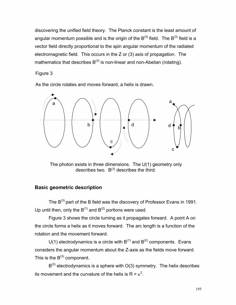
195

discovering the unified field theory. The Planck constant is the least amount of

angular momentum possible and is the origin of the B(3) field. The B(3) field is a

vector field directly proportional to the spin angular momentum of the radiated

electromagnetic field. This occurs in the Z or (3) axis of propagation. The

mathematics that describes B(3) is non-linear and non-Abelian (rotating).

Basic geometric description

The B(3) part of the B field was the discovery of Professor Evans in 1991.

Up until then, only the B(1) and B(2) portions were used.

Figure 3 shows the circle turning as it propagates forward. A point A on

the circle forms a helix as it moves forward. The arc length is a function of the

rotation and the movement forward.

U(1) electrodynamics is a circle with B(1) and B(2) components. Evans

considers the angular momentum about the Z-axis as the fields move forward.

This is the B(3) component.

B(3) electrodynamics is a sphere with O(3) symmetry. The helix describes

its movement and the curvature of the helix is R = κ2.

Figure 3

As the circle rotates and moves forward, a helix is drawn.

a

b

c

d

a

b

c

d

The photon exists in three dimensions. The U(1) geometry onlydescribes two. B(3) describes the third.

196

We saw this in Chapter 9 with curvature R and the Compton wavelength.

The B(3) field is a longitudinal photon, called the Evans photomagneton. It

is a phaseless magnetic field. It can be described by:

B(3)* := i g A(1) x A(2)

where g = e/ћ for one photon and A(1) = A(2)* is the transverse vector potential.

This can be developed further. Evans gives the magnetic field components:

Bcij = B(0) (qa

i qbj - qa

j qbI)

and the electric field components:

Ecoj = E(0) (qa

o qbi - qa

i qbo)

Note that the structure is that of the wedge product.

In the older view of gravitation, the electromagnetic field was a structure

imposed on flat spacetime. This viewpoint is known to be incorrect since

Figure 4 Basic Geometry

B(3) gives thelongitudinal

component of theelectromagnetic

field.

B(1)

B(2)

B(3)

y

x

z

A B

A B

+

-

SPACETIME

197

spacetime curves and twists, but until the Evans equations a method for

describing electromagnetics in four-dimensional curved space was unknown.

Now the accepted viewpoint must be that the electromagnetic field is also

a manifestation of spacetime described by an equation similar to Einstein’s

symmetric field equation, Rµν - ½ Rqµν = kTµν.

While the gravitational field is described by the symmetric Einstein field

equation, the electromagnetic field is described by the antisymmetric metric dual

to the symmetric metric. The existence of a symmetric metric and an

antisymmetric metric – curvature and torsion – is the concept that allows this

description.

The magnetic and electric fields in special relativity have circular U(1)

symmetry and are seen as entities on flat spacetime. In general relativity we

know spacetime is curved. In the unified field theory we see that

electromagnetism is turning spacetime. This is depicted in Figure 5.

The electromagnetic field is spinning spacetime.

Figure 5 Gravitation and Electromagnetism

B

E

B

E

Curved Spacetime

Curved, Turning,and Torqued

ElectromagneticSpacetime Field

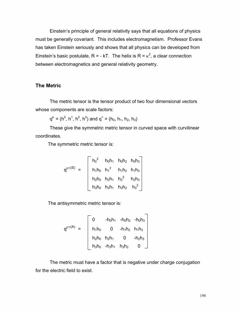
198

Einstein’s principle of general relativity says that all equations of physics

must be generally covariant. This includes electromagnetism. Professor Evans

has taken Einstein seriously and shows that all physics can be developed from

Einstein’s basic postulate, R = - kT. The helix is R = κ2, a clear connection

between electromagnetics and general relativity geometry.

The Metric

The metric tensor is the tensor product of two four dimensional vectors

whose components are scale factors:

qµ = (h0, h1, h2, h3) and qν = (h0, h1, h2, h3)

These give the symmetric metric tensor in curved space with curvilinear

coordinates.

The symmetric metric tensor is:

h02 h0h1

h0h2 h0h3

qµν (S) = h1h0 h12 h1h2 h1h3

h2h0 h2h1 h2

2 h2h3

h3h0 h3h1 h3h2 h3

2

The antisymmetric metric tensor is:

0 -h0h1 -h0h2 -h0h3

qµν (A) = h1h0 0 -h1h2 h1h3

h2h0 h2h1 0 -h2h3

h3h0 -h3h1 h3h2 0

The metric must have a factor that is negative under charge conjugation

for the electric field to exist.

199

Then the complete electromagnetic field tensor is the well-known tensor:

0 -E1 -E2 -E3

E1 0 -B3 B2

Gµν = E2 B3 0 -B1

E3 -B2 B1 0

The B field components are a rotating metric with antisymmetric metric

components.

Comparison of the two matrices qµν (A) and Gµν show that the signs are the

same and if one were to work them all the way out, they describe the same

rotation.

The Principle of General Relativity has been applied in the equations of

the B(3) field. The magnetic field is a metric (an antisymmetric metric tensor) that

rotates and translates.

There are three components of the B field. Two are circularly polarized

phase dependent complex conjugates perpendicular to the direction of

propagation. These are the B(1) and B(2) fields. There is one phase independent

component in the direction of propagation. This is the B(3) field.

The magnetic field components are related by the B Cyclic Theorem of

O(3) electrodynamics. The electric field components can also be defined in

terms of the rotation generators of the O(3) group. A metric describes the

electric components that also rotate and translate and is perpendicular to the

magnetic field. The metric is used to define the magnetic fields, B(1), B(2) and B(3)

of O(3) electrodynamics. The O(3) electromagnetic field has been derived from

curved space time and geometry.

Professor Evans’ analysis shows that his formulations lead to the

Coulomb, Gauss, Faraday, and Ampere-Maxwell equations. The B(3) field of

O(3) electrodynamics is responsible for interferometry, the Aharonov Bohm and

Sagnac Effects, the Berry Phase and all topological and optical effects.

200

Mass and spin characterize all particles and fields. The origin of the

Planck constant in General Relativity is explained and is shown to be the least

amount possible of action, angular momentum or spin in the universe.

In Professor Evans’ words, “We can also now identify ‘higher symmetry

electrodynamics’ as ‘generally covariant electrodynamics’, i.e. electrodynamics

that is indicated by the Principle of General Relativity, that all theories of natural

philosophy (including electrodynamics) must be generally covariant, i.e. theories

of general relativity.”

Given that gravitational curvature is related to electromagnetic spin, we

may be able to directly convert one form of energy to the other. This needs to be

determined in experiments to see if the effect is large enough.

Electromagnetic energy resides in the Evans spacetime (Riemannian

vacuum with Cartan torsion) without the presence of radiating electrons. We

may be able to tap this energy, which is a manifestation of curvature. Vacuum

electromagnetic energy is zero if and only if R is zero, and this occurs only in flat

spacetime, in which there are no fields of any kind (gravitational,

electromagnetic, weak or strong).

Summary

The development of the B(3) field is highly technical. A good source for

further study is Professor Evans’ Lecture Notes 1 and 2 that are available on

www.aias.us and the book Generally Covariant Unified Field Theory, (M.W.

Evans, Kluwer, Dordredt, 2004).

Starting with geometry Dr. Evans has taken the metric vectors which are

written as antisymmetric rank two tensors and then developed tensors written in

the complex circular basis to arrive at electromagnetism.

More simply stated, starting with Einstein’s geometry of our spacetime it

has been shown that electromagnetism is also described.

201

The B(3) field is the fundamental longitudinal and phaseless magnetic field

component of electromagnetic radiation in general relativity. The B(3) field can be

derived from general relativity and it is necessary to use the B(3) concept to

obtain generally covariant – reference frame free – electromagnetics.

The photon has mass as inferred by Einstein and de Broglie, and their

followers.

The metric that we label Evans spacetime has Einstein’s curvature and

Cartan’s torsion. The effects could be large enough to produce electromagnetic

power from gravitational curvature.

202

Chapter 12 Electro-Weak Theory

Problems cannot be solved at the same level of awareness that

created them.

Albert Einstein

Introduction

In this chapter the Evans Lemma is used to understand the masses of the

weak field bosons and to develop electro-weak theory without the concepts used

in the standard model. Electro-weak refers to the unification of the

electromagnetic and weak forces. The weak force holds some particles together.

For example, the isolated neutron and the muon transform after short times into

other particles. The neutron becomes a proton plus an electron plus an anti-

neutrino. The muon becomes a muon-neutrino.

The present standard model uses concepts like spontaneous symmetry

breaking and the Higgs mechanism, and it compensates for infinities due to zero

volume particles using renormalization. The path integral method is used for

calculating probabilities. The standard model uses the Higgs mechanism to

adjust the masses of the particle, but the Higgs particle has not been found in

experiments. The standard model uses adjustable, ad hoc parameters to gain

agreement between theory and experiment. These can accurately predict results

of most experiments however they are flawed at the theoretical level.

The W and Z bosons mediate the weak nuclear force.

Use of the Evans equations gives solutions from first principles in terms of

basic constants of physics and is to be preferred. It is simpler and explains

more.

203

General relativity is generally covariant and the existing standard model is

not generally covariant – it is a theory of special relativity that approximates

general relativity and is incomplete since the electromagnetic, strong, and weak

forces are not generally covariant – effects of gravitation cannot be predicted.

General covariance is a fundamental requirement of physics. Without

covariance, the laws of physics would vary in different reference frames.

The Evans Lemma is:

qaµ = R qa

µ (1)

where the eigenfunction is the tetrad qaµ. The values of R will be real

observables in our universe.

The Principle of Least Curvature is:

R0 = - (mc/ћ)2 (2)

This is valid in the limit of special relativity with flat spacetime. This is the limit of

the smallest value of R, scalar curvature, for a given mass. Mass m is adjustable

in equation (2) for c and ћ are, as far as we know, fundamental constants. R the

curvature is then fixed for any given mass.

The Compton wavelength of a particle is:

λ0 = ћ/ mc (3)

This is the wavelength of a photon with the same energy as the mass of a

particle with mass m. Using equations (2) and (3) one sees that the least

curvature of a particle or spacetime is R0 = (1/ λ0 2). The DeBroglie equation is

the same as the Compton equation with v the velocity of a particle instead of c.

See Chapter 9 for discussion.

Using Einstein’s index contracted field equation, R = - kT and the Evans

Lemma above, leads to the Evans Wave Equation, ( + kT) qaµ = 0.

The wave equation in terms of the least curvature is:

( + (mc/ћ)2) qaµ = 0 (4)

where qaµ is a tetrad, spinor, matrix, vector, or other as necessary.

204

For present purposes the following definitions (that are not universally

agreed upon) will suffice. void is true nothing. Vacuum is the special relativistic

Minkowski flat spacetime that approaches zero curvature and zero torsion. Real

spacetime can never become perfectly flat since where there is energy, there is

Figure 1 Tangent Gauge Space and Normal Curved Space

Curved space and index space.The index is the tangent space

of general relativity and isidentical to the gauge space of

quantum mechanics.

The index space of basisvectors is needed to performcalculations of real values ofcomponents. This must be a

linear space to accomplishcalculations.

µ

Index, a

Index and base manifold arespinning with respect to one

another.

µ

Index, a

X0

X1 X2

X3

The index space is like a snapshot at any one set of conditions.

205

curvature. Non-Minkowski or Riemann spacetime is the curved universe of

Einstein’s general relativity. It has only a symmetric metric giving distances.

Evans spacetime is curved and torqued. It is the real spacetime of our universe

with symmetric and antisymmetric metric. The antisymmetric metric allows for

electromagnetism. It could be as tenuous as the space far between galaxies or it

could be as dense and turbulent as the region in a particle or near a black hole.

Curvature and torsion are clearly recognized as present.

Eventually it may be that the terms twisting, turning, spinning, rotating will

have differences in connotation. For now, they are essentially the same thing.

Spin is defined by the tetrad with and without the presence of gravitational

curvature. The real spacetime base manifold and the tangent bundle are

spinning with respect to one another. If gravitation is not present then the base

and the bundle are both Minkowski spacetimes. There is compressibility due to

the energy density of velocity, but the spacetime is flat – gravitation is ignored.

See Figures 1 and 2.

Figure 2 In Special Relativity and the Standard Model, Tangent Space and Base Manifold are Flat

In the weak field limit,the index space and thebase manifold are bothflat. They do not curveor rotate with respect to

one another. This isMinkowski spacetime.

µ

Index, a

206

Derivation of the Boson Masses

In the Evans development of the electro-weak theory, wave functions are

tetrads governed by the Evans Lemma, equation (1), and the particle masses are

eigenvalues of the lemma – the values of R. This indicates that the masses have

real physical occurrence. In this way, the equations derive from physical

geometry as required by Einstein’s general relativity.

In the standard model, particles are assumed initially massless and then

“spontaneous symmetry breaking” occurs and the Higgs field-particle gives them

mass. The neutrino has no mass in the standard theory. The complexity is

unnecessary and it has been shown that the neutrino does have mass.43 Any

patch to the standard model to explain this is another unnecessary complication.

Equation (2), the Evans Principle of Least Curvature, is simpler and is

based on known constants. In addition, the Evans development is covariant and

can predict actions in different gravitational fields.

The Evans equations show that mass is defined by spacetime geometry –

the curvature R. And the masses of the electron and all particles are minimum

curvatures or minimum eigenvalues of equation (2).

RL = - (mLc/ћ)2 (5)

Where the superscript L indicates the electron.44

Waµ = R Wa

µ (6)

43 See http://neutrino.phys.washington.edu/~superk/sk_release.html The Super-Kamiokande experiment found evidence for non-zero neutrino mass. 44 Actually the left electron but we are leaving out a lot of detail in this explanation.

We see here that the curvature of a particle in general relativity is

expressed in quantum mechanics terms. The curvature is proportional to

the mass. The electro-weak interactions are described by curvature in

the Evans’ generally covariant approach. That is, quantum (electro-

weak) interactions are described in terms of general relativity (curvature)

in the unified field theory.

207

Here Waµ is a tetrad of the Weak field and

Waµ= W(0) qa

µ (7)

with W(0) a scaling factor.

The mass of the three electroweak bosons, the Z and two W particles, can

be derived from the Evans equations without the use of the Higgs mechanism

using the Evans Lemma and the Dirac equation. Experiments have given

energies (masses) of 78.6 GeV/c2 and 89.3 GeV/c2 for the bosons.

In the standard theory the bosons get mass from an equation with η the

Higgs mechanism which is adjusted to find the experimental results using

equations of the form:

L1 = g2 η2((W1µ)2 +((W2

µ)2)/4 (8)

Where g is a coupling constant and W is the boson. This leads to:

m2 = g2 η2/2 (9)

Ignore all the terms but m the mass of the boson and η the Higgs

“particle.” Higgs has not been found in nature, rather it is predicted based on the

other known values. As it happens Higgs can be replaced by Evans minimum

curvature value. Evans equations of the form:

m2 = ћ2/4c2 ((W1

µ)2 +((W2µ)2) (10)

are found where use of the Higgs is unnecessary since the minimum curvature is

the same thing and replaces Higgs. However the minimum curvature is based

on fundamental constants of physics, ћ and c in equation (2). Boson masses are

replaced by spacetime curvatures. This is a technically superior method.

The results of the calculations are the experimentally observed masses of

78.6 GeV/c2 (W) and 89.3 GeV/c2 (Z).

It is virtually impossible for this calculation to arrive at the boson masses if

the equations used were not correct. From fundamental constants the boson

masses are found.

208

Particle Scattering

Figure 3 shows the basic process of particle scattering when two fermion

particles collide. Conservation of energy and momentum must be maintained. In

Evans formulation, it is expressed as conservation of curvature must be

maintained. This is the same thing, but in the more basic concept of curvature

since energy and momentum are forms of curvature. p indicates a particle’s

momentum

The law of conservation of momentum is followed in all collisions. While

the total kinetic energy, Ek, can be converted to new particles, the momentum is

conserved separately. Figure 3 shows the basic equations. Note that p1 is not

typically equal to p3 nor p2 to p4. It is the sums that are equal. Total energy in

equals total energy out. Total momentum in equals total momentum out.

Figure 3 Momentum Exchange

k

p1 + p2 = p3 +p4

p1 + k = p3

p2 - k = p4

p1p2

p3 p4

k is the bosonp indicates the momentum

of the particles

The process can be written in the form:

f( k, m1 ) pb1 = f( m3 ) pb

3 = 0 (11)

f( k, m2 ) pb2 = f( m4 ) pb

4 = 0 (12)

where f is some function, k is the boson (energy exchanged) , m1 to 4 are the

masses of the particles in Figure 3, and pb1 to 4 are wave functions which are

209

tetrads in differential geometry. The wave functions pb3 (and pb

4) are that of the

particles after picking up (and losing ) momentum mediated by the boson k.

Equation (11) and (12) state that there is a function of the boson energy k

and m the mass of the particle times the wave function which is conserved.

There is no creation or disappearance of momentum. The boson is also

governed by an Evans equation of the form:

f( mk ) kbi = 0 (13)

where mk is the mass of the boson and kbi is the wave function of the boson

before colliding with the fermion. Equation (13) is derived from the wave

equation:

( + (mkc/ћ)2) kbι = 0 (14)

This is seen as a form of the now familiar Evans wave equation.

Figure 4

Particle scattering seen as curvatures

P1 + k + P2 - k = P3 + P4

P1P2

P3 P4k

Collisions between particles are governed by two laws: one, conservation

of momentum, and two, conservation of mass-energy. Conservation of the mass

energy is separate from the momentum; each is conserved separately.

Equations (10) to (14) replace standard model equations producing the same

results, but the Evans equations use fundamental constants. Two simultaneous

210

equations can describe any scattering process. These are covariant and transfer

to any gravitational system.

The test of any theory is not that it is renormalizable, but rather that it is

generally covariant as Einstein stated. See Figure 5.

Figure 5 Equations in the Tangent Bundle

The Evans equations arewritten in the tangentbundle space and aretherefore generallycovariant.

Curved space

Index SpaceTangent Bundle

µ

X0

X1 X2

X3

Waµ = R Wa

µ

X 0

X 1

X2

X 3

Curved space

µ

Basis Vectors

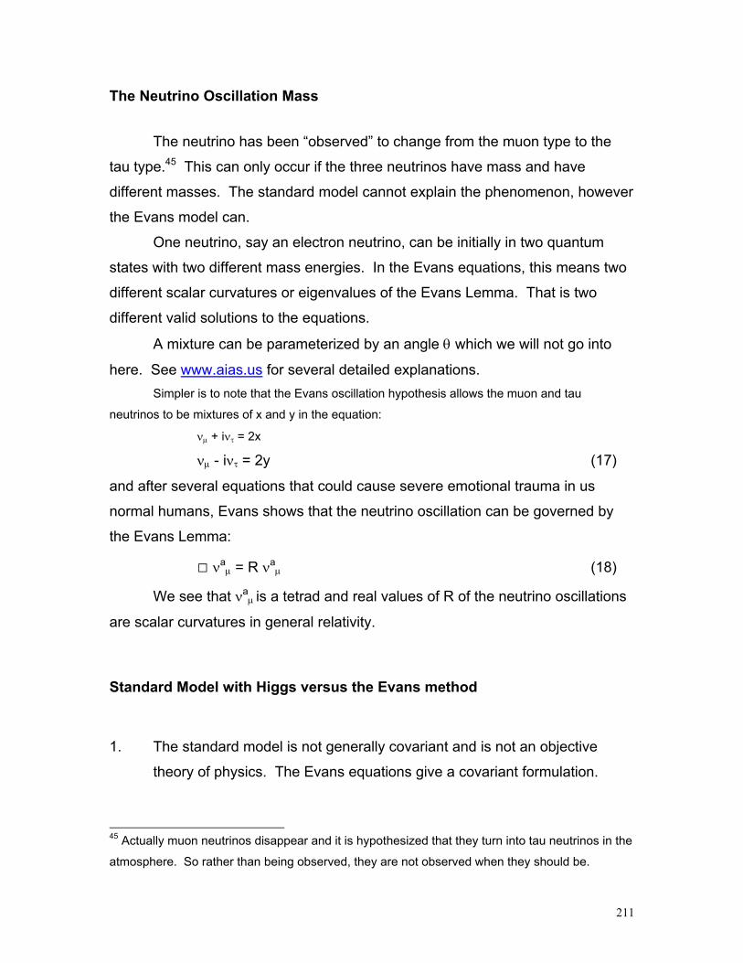
211

The Neutrino Oscillation Mass

The neutrino has been “observed” to change from the muon type to the

tau type.45 This can only occur if the three neutrinos have mass and have

different masses. The standard model cannot explain the phenomenon, however

the Evans model can.

One neutrino, say an electron neutrino, can be initially in two quantum

states with two different mass energies. In the Evans equations, this means two

different scalar curvatures or eigenvalues of the Evans Lemma. That is two

different valid solutions to the equations.

A mixture can be parameterized by an angle θ which we will not go into

here. See www.aias.us for several detailed explanations. Simpler is to note that the Evans oscillation hypothesis allows the muon and tau

neutrinos to be mixtures of x and y in the equation:

νµ + iντ = 2x

νµ - iντ = 2y (17)

and after several equations that could cause severe emotional trauma in us

normal humans, Evans shows that the neutrino oscillation can be governed by

the Evans Lemma:

νaµ = R νa

µ (18)

We see that νaµ is a tetrad and real values of R of the neutrino oscillations

are scalar curvatures in general relativity.

Standard Model with Higgs versus the Evans method

1. The standard model is not generally covariant and is not an objective

theory of physics. The Evans equations give a covariant formulation.

45 Actually muon neutrinos disappear and it is hypothesized that they turn into tau neutrinos in the

atmosphere. So rather than being observed, they are not observed when they should be.

212

2. The gauge space used in the standard theory is an abstract mathematical

device with no physical meaning. A number of concepts are ad hoc

constructions. The Evans method uses differential geometry and

Einstein’s concept of curvature.

3. The Higgs mechanism is a loose parameter introduced by an abstract

mathematical model of the Minkowski vacuum with no physical meaning.

The Higgs particle-field-mechanism is a mathematical parameter found by

fitting data to known energies. The Evans equations use the concept of

minimum curvature which is based on fundamental constants.

4. Renormalization is used in the standard model. This sets an arbitrary

minimum volume of a particle to avoid infinities. The formula based on the

Evans equations is a concrete method. That is V = k/m (ћ/c)2 as given in

Chapter 9. Both Einstein and Dirac rejected renormalization. It was a

clever method to set minimum volumes while they were still unknown.

However it is a most complicated process that was necessary only

because of the incomplete standard model.

Generally Covariant Description

The first generally covariant description of the transmutation of the muon

into the muon-neutrino was given in notes placed on the www.aias.us website.

This was:

(iћγa (∂a + igWa) − mµc)µb = (iћγa ∂a - mµc)νb ) = 0 (19)

This is a landmark equation although unlikely to become quite as famous

as E = mc2.

213

Chapter 13 The Aharonov Bohm (AB) Effect

General relativity as extended in the Evans unified field theory is needed for a correct understanding of all phase effects in physics, an understanding that is forged through the Evans phase law, the origin of the Berry phase and the geometrical phase of electrodynamics observed in the Sagnac and Tomita Chiao effects. Myron W. Evans

Phase Effects

A simple explanation of a phase effect is shown in Figure 1. The sine

wave that is expected is not found in certain experiments.

Explanations to date of why they occur have been awkward and

questionable. Evans shows that his generally covariant equations are simpler

and demonstrate the causes of phase effects. The mathematics involved in

phase effects and descriptions of phenomena like the AB effect are difficult and

beyond what we can deal with in any detail here. However, the effects can be

discussed without mathematics details.

Expected PhasePhase shifted

Figure 1 Phase Effects

Phase

We assume that a beam of photons or electrons is shot at a screen. An

interference pattern will occur as shown in Figure 3. For an electromagnetic field

214

the phase law tells us that the phase is a function of potential voltage and the

area of the beam or the magnetic field strength and the area. That is:

Φ = function of (A • dr ) = f( B(3) • k dAr )46 (1)

where A is potential voltage, B(3) is the magnetic field (both are directed in the Z

axis of propagation) and Ar is the area of a circle enclosed by the beam. The arc

length of the circle as it turns becomes that of a helix as shown in Figure 2.

Figure 2

a

b

c

d

a

b

c

d

The diameter of a circle equals 2πr. The distance that this describes whenmoving forward is not a full circle. Rather the arc length of the helix is drawn.

Z

The sine wave describes the circular motion shown below.

46 Actually, Φ = exp( ig ∮ A(3) • dr ) = exp( ig ∮ B(3) • k dAr ) := exp( i ΦE). For matter fields, Φ = function of (κ • dr ) = f(κ2 • dAr )46 where κ is the wave number (inverse wavelength).

215

The curvature of the helix is defined as R = κ2. We thus see a geometric

curvature in relativity expressed in the description of phase. The helix in Figure 2

is the baseline of the electromagnetic field.

Spacetime itself spins. Both electromagnetic and matter waves are

manifestations of spacetime itself.

The angle Θ through which light is rotated out of phase originates in the

Evans phase of unified theory. This is:

Θ = κ ∮ ds = R ∫dAr (1)

Here κ is wave number, ds is the invariant line element of relativity, R is

curvature, and Ar is the area enclosed by the beam.

.

The Aharonov Bohm Effect

The Aharonov Bohm Effect is a shift in the interference pattern of two

electron beams in a Young interferometer. An explanation is shown in Figures 3

and 4. Electrons pass through a double slit and an interference pattern builds

up. Classical quantum mechanics predicts a certain pattern which is found in

experiments and designated C in the figures.

When an enclosed magnetic field is placed between the slits, indicated ⊚, classical quantum mechanics predicts no change in the pattern. The magnetic

field is totally enclosed in a metal case and cannot influence the electrons.

However, the pattern shifts as designated AB in Figure 4. (It is greatly

overemphasized.)

The only explanation in the past was that the vacuum is a multiply

connected topology and complex mathematics was necessary to show the

reason for the AB effect. See Figure 5. This is an overly complex and

unprovable solution. The simple answer is that the field does extend beyond the

barrier.

216

Figure 3 Double slit experiment

ElectronSource

Two slit barrier

Electronbeams

Expectedinterference

pattern

C

Figure 4 AB Effect

ElectronSource

Twoslit

barrier

Electronbeams

AB

C

Enclosedmagnetic

field

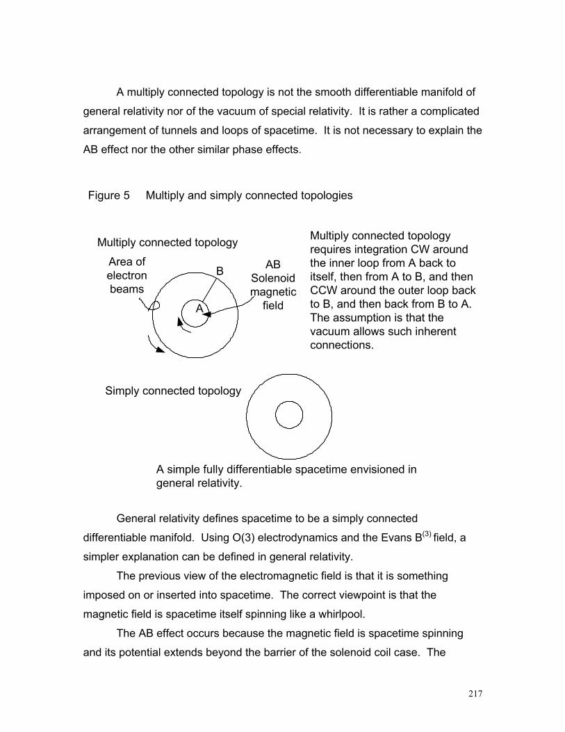
217

A multiply connected topology is not the smooth differentiable manifold of

general relativity nor of the vacuum of special relativity. It is rather a complicated

arrangement of tunnels and loops of spacetime. It is not necessary to explain the

AB effect nor the other similar phase effects.

Figure 5 Multiply and simply connected topologies

Area ofelectronbeams

ABSolenoidmagnetic

fieldA

B

Multiply connected topology Multiply connected topologyrequires integration CW aroundthe inner loop from A back toitself, then from A to B, and thenCCW around the outer loop backto B, and then back from B to A.The assumption is that thevacuum allows such inherentconnections.

Simply connected topology

A simple fully differentiable spacetime envisioned ingeneral relativity.

General relativity defines spacetime to be a simply connected

differentiable manifold. Using O(3) electrodynamics and the Evans B(3) field, a

simpler explanation can be defined in general relativity.

The previous view of the electromagnetic field is that it is something

imposed on or inserted into spacetime. The correct viewpoint is that the

magnetic field is spacetime itself spinning like a whirlpool.

The AB effect occurs because the magnetic field is spacetime spinning

and its potential extends beyond the barrier of the solenoid coil case. The

218

equations using torsion clearly and simply explain the AB effect. Spacetime is

continuous and effects extend beyond the barrier.

The Evans unified field theory gives solutions for a number of topological

phase effects that are similar or essentially the same as the AB effect. These

include the electromagnetic Aharonov Bohm effect (EMAB), Sagnac effect,

Tomita-Chiao effect, and Berry phase factor. The Tomita-Chiao effect is a shift in

phase brought about by rotating a beam of light around a helical optical fibre.

This is the same as the Sagnac effect with several loops, and is a shift in the

Cartan tetrad of the Evans unified field theory. Similarly, the Berry phase of

matter wave theory is a shift in the tetrad of the Evans unified field theory.

In the Evans’ theory the effects are simple to understand and describe.

They are all related to the Inverse Faraday Effect and use B(3) electromagnetics

and O(3) electrodynamics. On the other hand, the U(1) Maxwell-Heaviside

theory cannot explain these effects except by torturous logical inversions.

The Helix versus the Circle

Evans’ papers give more than just an explanation of these effects. He

shows that using differential geometry that the received explanations make

incorrect assertions. Multiply connected spacetimes do not obey the rules that

physicists have given them to explain the AB effect.

In this book we have avoided differential geometry since it is not simple

mathematics. In his papers Evans often starts with a physics equation, restates

it in differentials, finds a truth in geometry, and then restates the physics equation

giving new insights. The following is paraphrased from Evans:

The Stokes theorem shows that ∮δS dχ :0. However, the

conventional description of the AB effect relies on the incorrect assertion

that ∮δS dχ :≠ 0. This violates the Poincaré lemma. In differential

geometry, the lemma is true for multiply-connected as well as simply-

connected regions. In ordinary vector notation the lemma states that, for

219

any function, ∇ x ∇χ := 0. The Stokes theorem and the Green theorem

are both true for multiply-connected regions as well as for simply-

connected regions. There is therefore no correct explanation of the AB

effect in Maxwell-Heaviside theory and special relativity.

Figure 6

The photon exists in four dimensions. The U(1) geometry onlydescribes three. B(3) gives three spatial plus time dimensions.

The diameter of a circle equals 2πr. The distance that this describes whenmoving forward is not a full circle. Rather the arc length of the helix is drawn.

a a'

c

a a'

c

As the circle rotates andmoves forward, a helix is

drawn.

Ordinary Stokes is a circle. The generally covariant Stokes is a helix.

a

b

c

d

a

b

c

dZ

The difference between the generally covariant Stokes theorem and the

ordinary Stokes theorem is the same as the difference between generally

covariant electrodynamics and the older Maxwell-Heaviside electrodynamics. In

220

Maxwell-Heaviside there is no longitudinal component of the photon. It describes

a circle. In Evans B(3) formulation the mathematics is that of a helix. See Figure

6. Maxwell-Heaviside special relativistic explanation is three dimensional while

Evans is four dimensional.

If the length Z were to equal 2πr, then the shape would be a straight line.

As it is, the implication is simply that the U(1) Maxwell Heaviside cannot describe

the physical process correctly and the O(3) formulation must be used and has

given correct answers to the AB and other effects.

Summary

There are phase shifts like the AB effect that require awkward

explanations in the standard model which receive simpler explanations in the

Evans formulation of general relativity. There is unification of electromagnetic

effects with curvature and torsion using the unified field theory.

221

Chapter 14 Geometric Concepts

We believe in the possibility of a theory which is able to give a complete description of reality, the laws of which establish relations between the things themselves and not merely between their probabilities...God does not play dice with the universe.

Albert Einstein

Introduction

There are developments that Evans makes in his papers that we have not

covered in this book. Some of the more geometrical are described briefly in this

chapter.

The Electrogravitic Equation47

The Evans wave equation is:

(+kT) qaµ = 0 (1)

where k is Einstein’s constant, T is the stress energy tensor, qaµ is the tetrad

which is the gravitational potential field.

The wave equation for electromagnetism is:

(+kT) Aaµ (2)

where Aaµ = A(0) qa

µ (3)

47 The descriptions here are taken from “Development of the Evans Wave Equation in the Weak Field Limit: The Electrogravitic Equation” by M.W. Evans et. al. See www.aias.us.

222

Aaµ is the electromagnetic potential field.48 A(0) is the electromagnetic potential

voltage. This is the Evans Ansatz - the proposed conversion from geometry to

electromagnetics.

If all forms of mass and energy are related through curvature, R, then an

equation should exist which gives us electromagnetism as a function of

gravitation. This fundamental ratio of charge e to mass m is in terms of the

electrostatic potential φ(0). φ(0) would be a scalar voltage with units of volts.

Then this equation should exist:

A(0) qaµ = φ(0) qa

µ (4) c2

Elsewhere it has been shown that the Evans wave equation becomes the

Poisson equation in Newtonian gravitation in the weak field limit. The well known

Poisson equation for gravitation is:

∇2φ = 4πGρ (5)

where φ is the gravitational potential in m/s2, G is the Newton gravitational

constant, and ρ is the mass density in kg/m3.

The acceleration due to gravity in units of m/s2 is:

g = ∇φ (6)

Similarly equation (2) becomes the Poisson equation for electrostatics in

the weak field limit:

∇2 (φ(0) φ) = 4πG(φ(0)ρ φ) (7)

The electric field is then described as:

E = 1 ∇(φ(0) φ) (8) c2

The factor 1/c2 is needed to adjust to S.I units.

Substituting equation (6) in equation (8) we see that:

E = φ(0) g (9) c2

48 This is a vector valued tetrad one-form within a Ĉ negative (charge conjugation) factor A(0).

223

This gives the electric field strength in terms of g. The field is in units of

volts per meter (or Joules per Coulomb per meter). It shows that there is a

mutually calculable effect between gravitation and electromagnetism. There is

one field, the electrogravitic field.

The effects will be difficult to test since they are quite small. Given two

one kilogram masses one meter apart charged with one Coulomb, the

gravitational force is 6.67 x 10-11 Newtons.

φ(0) is a fundamental voltage available from curved spacetime. There is an

electric field present for each particle and it originates in scalar curvature.

The effect may be important in black hole formation as the high degree of

torsion in both the mass and electrical potential in the spacetime being pulled into

a hole accelerates and collapses. When we have a test black hole we will be

able to confirm the effect.

The effect may be very important for extraction of energy from the

curvature of spacetime near our planet. If an array of receptors can be

developed, a low cost source of energy becomes available.

Principle of Least Curvature

In the flat Minkowski spacetime limit we saw in Chapter 9 that R

approaches (mc/ћ)2 and IR0I = 1/λ02. In this way we see that mass is expressed

as scalar curvature of spacetime. This is the Principle of Least Curvature. R

values here are eigenvalues of the Evans Lemma. Eigenvalues are real physical

results.

While the least curvature is defined by the rest mass, the particle can have

more curvature. If accelerated towards the speed of light, the particle would

have greater internal curvature. If put inside a strong gravitational field, the

curvature of the field and the curvature of the particle would be combined. The

reference frame of the particle would be compressed.

There are several implications. One is that particle mass is curved

spacetime. We have seen that the electromagnetic field is spinning spacetime.

224

Another is that a particle never travels in a straight line since the scalar curvature

of a straight line is zero. The least curvature of a particle is the least action

possible, ћ. In the final analysis, we find that everything in our universe is

spacetime. It is not simply that everything obeys the same rules, rather we see

the particle as a bit or region of highly curved spacetime. The particle

presumably has torsion also since it has a frequency.

Just what equation will be found to explain the particle masses remains to

be seen. There will be found some ratio or similar relationship between

curvature and torsion, and the masses of the basic particles.

Non-local Effects

The Evans unified field theory also explains the violation of the Bell

inequalities observed experimentally in the Aspect experiments, i.e. in regions

where there are no matter or radiated fields of any kind there are matter or

radiation potentials. These give rise to the "non-locality" of quantum mechanics

The spacetime curvature R in one location extends to others. This is not

action at a distance, but rather extended spacetime curvature. This offers an

explanation for seemingly simultaneous actions at a distance. Rather than

”entanglement” or “non-locality” as in quantum mechanics, we have a shift in

spacetime curvature.

The AB effect is explained by extension of spacetime torsion outside a

solenoid coil’s enclosure in Chapter 13. In the same exact manner the

gravitational attraction experienced by masses for one another are explained by

the extension of curvature outside the immediate volume of a particle. Each

mass is spacetime and it extends to infinity causing curved space. Differential

geometry shows that a seemingly local effect extends throughout spacetime and

cause “non-local” effects.

Differential geometry has a solution giving the cause for entanglement in

quantum mechanics. No satisfactory solution has been found in the existing

standard model.

225

EMAB and RFR

Magnetic, electric, and gravitational AB effects have been observed to

date. The electromagnetic AB effect has not yet been observed.

Evans proposes an experiment using what he calls the Electromagnetic

Aharonov Bohm effect (EMAB). The electromagnetic potential field was defined

in equation (3) as Aaµ = A(0) qa

µ . The field causes interaction of circularly

polarized electromagnetic radiation with an electron beam.

The magnetized iron whisker of the original AB effect can be replaced by a

circularly polarized radio frequency beam. The B(3) component of the radio

frequency field causes a shift in the fringe pattern of two interfering electron

beams. This has not been performed to date, but if successful it could open up a

new radar technology.

Similarly, radiatively induced fermion resonance (RFR) can be tested.

This would lead to a new type of imaging that would be much more accurate than

present MRI methods.

Calculations show that the phase shift using standard lasers at typical

power densities is unobservable.

The Inverse Faraday Effect is the orbital angular momentum given to

electrons in a beam by photons. This is explained by the Evans B(3) spin field.

For a beam traveling at low velocities the energy is:

EIFE = e ћ B(3) = e2A(0)2/2m = p2/2m (10)

where e is the charge of the electron, m is the mass of the electron, p = e A(0) is

its linear momentum. p2/2m is the kinetic energy. The energy given to the beam

is a directly proportional to the power density and inversely proportional to the

square of the angular frequency.

The equations describing this can be derived from differential geometry

and the B(3) field. The result is a known equation.

226

Differential Geometry

We have avoided differential geometry in this book up to now because of

its complexity. Once it is understood, it simplifies physics, but getting to that level

is not a common achievement.

However, even if it is not perfectly clear, a look at it is interesting.

The fundamentals of the unified field theory are based on these equations:

Tc = D ⋀ qc First Maurer Cartan structure relationship. The torsion form is defined as the covariant exterior derivative of the

tetrad. Here the indices of the manifolds, typically µ and ν are not included since

they are redundantly placed on both sides of the equation.

Rab = D ⋀ ωa

b Second Maurer Cartan structure relationship. This defines the Riemann form Ra

b as the covariant exterior derivative of

the spin connection, ωab.

Dq a = 0 Tetrad postulate.

D ⋀ Va = d ⋀ Va = ω ab ⋀ Vb

This defines the covariant exterior derivative.

Evans simplifies these to a form with the wave number and shows further

that R, scalar curvature, can be defined as the square of the wave number with

units of inverse meters squared. That is:

R := κ2 (11)

Then in order to derive physics from the geometry, Evans uses Einstein’s

postulate:

R = -kT (12)

R is geometrical curvature; kT is physics observation. Equation (3), Aaµ =

A(0) qaµ , is used to convert from asymmetric connections to electromagnetism.

The magnetic field in differential geometry is expressed as:

Ba = D ⋀ Aa (13)

227

The expressions in differential geometry look quite different from physics,

but the logic is straightforward and all fits together. In Evans’ words:

It is now known with great clarity that the interaction of these fields takes place through differential geometry: D ⋀ F = R ⋀ A (asymmetric Christoffel connection) …Here D ⋀ is the covariant exterior derivative containing the spin connection, R is the curvature or Riemann two-form, T the torsion two-form, q the tetrad one-form, F the electromagnetic field two-form and A the electromagnetic potential one-form. However, it is also known with precision that the Faraday Law of induction and the Gauss Law of magnetism hold very well. Similarly the Coulomb and Newton inverse square laws. So the cross effects indicated to exist in physics by the above equations of geometry will reveal themselves only with precise and careful experiments.

Fundamental Invariants of the Evans Field Theory

The fundamental invariants of the particle in special relativity are the spin

and the mass. Regardless of the reference frame, spin and mass will be

invariant and they completely define the particle. In pure mathematics these are

referred to as the Casimir invariants of the Poincaré group. The first is:

C1 = pµ p µ. = (mc/ħ )2 = IR0I (14)

which is rest curvature for the mass m.

Curvature R is then an invariant in differential geometry and in the Evans

unified field theory. And since the Evans Lemma gives us R as eigenvalues, we

have quantization of general relativity. The R values in the Evans wave

equation and Einstein’s postulate of general relativity are invariant observables of

unified field theory.

The second is:

C2 = m2 s(s+1) (15)

This is a description of spin and is also a fundamental scalar invariant. C2 is

shown to be similar to a structure invariant of differential geometry. In simple

terms, C2 is the spin invariant.

The analysis has been extended into general relativity from special

relativity.

228

. Using differential geometry, Evans identifies two types of invariants -

structure and identity. There cannot be a gravitational or electromagnetic field by

itself. The two will always be present together. It is unphysical to have one

disappear. However one can be very small and this still needs to be found by

experimentation.

The only quantity that enters into the essential Evans equations outside

differential geometry is the fundamental potential A(0) which has the units of volts

or J-s/C-m. A(0) = ћ/er0 where e is the proton charge and r0 is a fundamental

length in meters.

r0 = λc = ћ/mc. (16)

It is seen that the fundamental voltage is also a geometric property of spacetime.

Evans also shows that

mc = eA(0) = e(ћ κ0 / e) (17)

This shows that rest energy / c is the product of two C negative quantities;

these are e, charge, and A(0) which is voltage. For two different signs of charge,

the positive and negative, the equation always gives positive mass. This is the

experimental observation which has not had any theoretical foundation until now.

The eigenvalues, real solutions, of the tetrad are fundamental

invariants of unified field theory. Particles are solutions of the Evans

Lemma.

In the real universe there are always electromagnetic and

gravitational fields present together. Neither can disappear to exactly

zero.

229

Origin of Wave Number

Starting with the ansatz:

Aaµ =A(0) qa

µ (18)

This says the electromagnetic tetrad is voltage times the asymmetric tetrad.

Without covering the differential geometry equations that lead to all the

formulation here we find that the magnetic field B equals A(0) times a torsion form

indicated by T. That is:

B(0) = A(0) (T232 + iT1

32) (19)

And in the Maxwellian limit it is known that:

B(0) = κ A(0) (20)

where κ is the wave number, κ = ω/c, ω is the angular frequency, and c the speed

of light. From equations (19) and (20):

κ = T232 + iT1

32 (21)

The scalar curvature, R, is defined as:

R = κ2 which we can now see as a function of torsion T49

Processes in electrodynamics can therefore be described by the

components of the torsion tensor. It is well known that the dielectric permittivity

and the absorption coefficient in spectroscopy are defined in terms of a complex

wave number, so the process of absorption and dispersion becomes

understandable in terms of spacetime torsion.

Photon mass is defined by the Evans Principle of Least Curvature:

49 Actually Professor Evans gives us R = κ κ ∗ = (T2

32 )2 – (T132)2. We are simplifying here to

explain the basic ideas.

Equation (21) shows that the origin of wave number and frequency in electrodynamics

is the torsion of spacetime.

230

κ −−> 2π/λ0 = 2π mc/ћ (22)

Here λ0 = ћ/mc is the Compton wavelength and ћ = h/2π is the reduced Planck or

Dirac constant. If the photon mass is about 10-60 kg, the minimum wave number

is about 10-18 m-1, and

T 2π mc/ћ (23) The mass is the minimum value of the torsion tensor component T:

m = (ћ/ 2πc) (Tmin) (24)

What precise information about particles will be uncovered by these

equations is unknown as of this writing. However it would seem that

understanding of all the particles observed in experiments will be seen in terms

of curvature and torsion – gravitation and electromagnetism together.

Summary

Differential geometry is physics. This is Evans primary basis for

development of any number of equations in a variety of areas. The interaction of

the four fields in physics takes place through differential geometry.

A number of examples are given here in simplified form.

The electrogravitic equation shows that conversion of curvature to torsion

is likely possible and may lead to a new energy source.

Particles are curvature and torsion together with mass determining the

least curvature.

Entanglement in quantum mechanics is due to spacetime geometry.

The invariants of physics and the origin of mass and spin is differential

geometry. The analysis has been extended into general relativity from special

relativity showing another factor in unification.

The point that Evans makes is that geometry is physics.

231

Chapter 15 A Unified Viewpoint

Mass and energy are therefore essentially alike; they are only

different expressions for the same thing. The mass of a body is not

a constant; it varies with changes in its energy.

Albert Einstein, The Meaning of Relativity

Introduction

As of this writing physics is still in several theoretical camps and each is

certain that it has the greatest promise for success. We have general relativity

including Evans’ work, quantum mechanics in the standard model, and string

theory and its offshoots. The evidence so far indicates that the Evans

formulation is the only one that unifies gravitation and electromagnetism. It

shows that quantum mechanics emerges from general relativity. It is correct in

all its basic assumptions and it has been experimentally proven by a number of

effects which it predicts and explains and which the standard model cannot

explain.

The Evans Equations complete Einstein’s unification goal.

Further experimental verification will occur. That there will be corrections,

modifications, and clarifications is inevitable. However the basic concepts are

now drawn out and are quite clear. There will be more discoveries in the future

as physicists analyze older problems using the new methods, so this is certainly

not the end of the story.

232

This chapter reviews the material we have covered; adds more pictures,

mechanical analogies, and simplified relations; and considers some implications

that are a bit speculative.

The opinions here are not necessarily sanctioned by Professor Evans.

Any errors in this book, but especially in this chapter are this author’s.

Review

There are problems within special relativity, general relativity, and

quantum theory as they have stood in the past. Quantum theory is a theory of

special relativity. Neither quantum theory nor special relativity can deal with

spacetime gravitational effects. Einstein’s general relativity explains spacetime,

but it cannot adequately describe the other three forces within it. Each theory is

well developed to explain matters within its own area, but is disjointed from the

others.

The Evans field equation is the first insight into unification that Evans gave

us. From it Einstein’s gravitational field equation can be derived but also a new

equation of spinning spacetime that describes the electromagnetic field.

The metric of spacetime must be defined as having torsion and curvature,

T and R, to allow the turning of the electromagnetic field. Differential geometry

already defines this metric and appears to be sufficient for the task.

Geometrically T and R are the only forms necessary to describe

spacetime. The tetrad is the form that allows relations between different

spacetimes. These are not new concepts, but they are used now with a new

equation. Suddenly, the picture becomes much clearer.

From matrix geometry which is well developed, the tetrad is analyzed in

terms of its symmetry properties. A new concept occurs:

Symmetry indicates centralized potentials – spherical shapes. Gravitation

and electric charge are symmetrical.

233

Antisymmetry always involves rotational potentials – the helix. Magnetism

and a new form of gravitation are antisymmetric.

Asymmetry indicates both are contained in the same shape. This is our

universe’s spacetime metric or manifold. Any form of mass or energy always has

some of the other form however slight. Antisymmetric and symmetric curvature

and antisymmetric and symmetric torsion coexist. Gravitation and

electromagnetism should always be present together to some degree.

The chart at the end of Chapter 6 shows the connections between the

various uses of the Evans field equation.

The generally covariant field equations of gravitation and electrodynamics

in tetrad form are:

Raµ – ½ Rqa

µ = kTaµ

Evans (1)

Rµν – ½ Rgµν = kTµν Einstein (2)

qaν Λ (Rb

ν - ½Rqbµ) = kqa

ν Λ Tbµ

Torsion (Evans) (3)

In Chapter 7 Evans wave equation is discussed. This is an equation that

is as much quantum theory as general relativity. It emerges from general

relativity and it quantizes general relativity. The wave equation is ( + kT)qaµ =

0 .

can be considered half torsion and half curvature. kT is Einstein’s

constant times the stress energy tensor. It is the energy density of a system –

particle, magnetic field, electric charge, or antisymmetric gravitation.

The tetrad can be expressed in a variety of ways and this has great power

to allow unification. The tetrad can be a scalar, vector, spinor, etc. That allows

the same equation to describe all the forces (fields) of physics and to be an

The Evans Wave Equation ( + kT)qaµ = 0 is derived from the Evans

field equation and is the unification equation. It is as rich in quantum

applications as Einstein’s field equation is rich in gravitational applications.

234

equation in special relativity, quantum mechanics, and general relativity. See

Figure 1.

The mathematical separation of the asymmetric tetrad into symmetric and

antisymmetric parts indicates more about the basic forces. The forces are

representations of symmetries.

This is a wonderful example of the interaction between mathematics and

physics. Since the tetrad is known to be valid in both mathematics and physics,

and since the tetrad is properly described by a matrix in geometrical

mathematics, it is also a proper description in physics. This follows Einstein’s

and Evans contention that physics is geometry.

Subjects are discussed which in the past were seen as primarily quantum

mechanics, but which can now be looked at in relativistic terms.

The Dirac and Klein-Gordon equations give us the formula for the mass-

volume relationship in terms of the basic constants c, ħ, and G.

qaµ( + kT) = 0a index indicates internal spaceµ indicates the 4-dimensionalRiemann curved spacetime

If a scalar, gµν, then R=-kT is therotation generator for a single

particle wave equation - the Klein-Gordon equation.

q

A spinor leads to the Diracequationψ

Aaµ

Saµ

Weak field

Electromagneticfield

Strongfield

Waµ

eaµ

Gravitationalfield

Figure 1 The tetrad and the forces of physics

aµ

aµ

235

We know energy density increase is accompanied by a decrease in the

volume of any spacetime system as perceived from a low energy density

reference frame. Reference frames contract in special relativity as they

approach the speed of light. Wavelength decreases in electrodynamics as

frequency increases with energy increase. The neutron star and black hole

decrease in volume at certain mass concentrations. The black hole and the

particle obey the same equation. But so does the magnetic field, the electron,

and antisymmetric gravitation. Now we see that a minimum volume exists. The

black hole is not a point – it is a dot. There are no singularities. And we have the

formula for calculations. The volume shrinks, but never to zero.

mV0 = k ħ2 / c 2 (4)

Heisenberg uncertainty is not required and in unified field theory we have

causal quantum mechanics. The Evans B(3) spin field is described and explains

the Inverse Faraday Effect. O(3) electrodynamics is derived from general

relativity using the Evans equations and describes spinning spacetime. It can be

viewed as an intermediate theory between the standard theory and full unification

theory.

Electroweak theory is discussed and one example of how Evans attacks

the problem using unified field theory rather than quantum theory shows the

power of the Evans equations. The Z and W bosons are shown to be described

as forms of curvature. The Higgs mechanism is not needed.

Analysis of the AB effect shows the concept of spinning spacetime as the

electromagnetic field. Spacetime extends beyond an immediate region and is

the key concept in understanding entanglement. “Non-local” effects do not

occur. Rather, entanglement is a spacetime effect.

Evans uses differential geometry applied to physics problems. Einstein

developed general relativity using Riemann geometry and Evans developed the

unified field theory using differential geometry. He is not the first to use it, but he

succeeds in unification and uses geometry to explain it.

Only two concepts besides differential geometry are necessary to use to

develop the equations of unification. One is the ansatz using conversion voltage

236

A(0) to turn the tetrad into electromagnetics. The other is Einstein’s postulate R =

kT. This equates geometry on the left side with physics on the right side. If one

reads Evans papers in sequential order it is seen that in the beginning he started

with physics, found differential geometry allowed proper development of

equations, and reformulated the physics in terms of differential geometry. In the

end he clearly declares physics is geometry, just as Einstein declared.

Curvature and Torsion Our universe requires curvature and torsion for unification of gravitation and

electromagnetism. The Evans spacetime metric has both. The metric in Evans’

extension of general relativity is asymmetric - it has symmetric and antisymmetric

components. This is the difference between it and Einstein’s general relativity

which has a symmetric Riemann metric with curvature alone. Evans has added

the antisymmetric torsion to unify the previously separate components . All

phenomena can be described using curvature and torsion. Differential geometry

and physics are intimately related, if not identical constructs. The strongest

statement is that what is true in differential geometry is true in physics. There are

certain aspects that will be more physical than others and clearly defining them

will lead to more understanding.

That curvature is gravitation and torsion is electromagnetism is not

controversial. Evans tells us that curvature and torsion always exist together to

some degree. The one can be converted to the other. Curvature in geometry is

the 1st curvature and torsion is the 2nd curvature.

Mathematics = Physics

The formation of equations with “Geometric Concept = Physics Equation”

is basic in relativity and Evans’ unified field theory. This is seen in Einstein’s

postulate R = -kT. R is geometry, -kT is physics.

237

G qaµ = kT qa

µ. (5)

Is one formulation of the Evans field equation. By breaking the tetrad, qaµ., into

symmetric and antisymmetric parts, a mathematical operation, a new window into

physics opens. The inner structures of Einstein’s and Evans’ field equations as

well as that of curvature and torsion are revealed.

qaµ

= qaµ

(S) + qaµ

(A) (6)

And since the electromagnetic potential field is defined:

Aaµ

= A(0) qaµ (7)

where A(0) is voltage, then we find symmetric and antisymmetric parts of it

also:

Aaµ

= A(0) qaµ

= Aaµ

(S) + Aaµ

(A) (8)

We can then expand or redefine R = - kT to:

R1 qaµ

(S) = - kT1 qaµ

(S) (9)

R2 qaµ

(A) = - kT2 qaµ

(A) (10)

R3 Aaµ

(S) = - kT3 Aaµ

(S) (11)

R4 Aaµ

(A) = - kT4 Aaµ

(A) (12)

where T is the energy momentum tensor. T1 is symmetric gravitation. T2 is anti-

symmetric gravitation. T3 is symmetric torsion indicating electrostatics, and T4 is

anti-symmetric torsion giving electromagnetism.

On the left side of each equation is the mathematical formulation of

curvature. On the right side of each equation is the physics formulation of stress

energy density.

Where Einstein had only the symmetric form of curvature of equation (7) –

the gravitational field - the Evans Equations indicate that there are four potential

fields and four types of energy momentum.

All four potential fields are interconvertable and all forms of energy are

interconvertable and:

Taµ

= Taµ

(S) + Taµ

(A). (13)

238

The stress energy can take four forms also. In addition the tetrad can

represent other forms such as the spinor or SU(N) symmetries leading to the

strong field particle or weak field radiation.

The Tetrad and Causality

The tetrad links two reference frames. It absorbs differences and

translates vectors in one to those in the other. The base manifold is curved and

torqued spacetime; the index is Euclidean spacetime.

The tetrad and the concept of moving frames as an alternate description

of general relativity was invented by Elié Cartan. The tetrad is a key concept in

expanding the field and wave equations into greater understanding.

The tetrad is a vector valued one-form in differential geometry. It provides

the connections between the curved and torqued spacetime of our universe with

the flat tangent mathematical space where we hold our vectors in order to

calculate transformations from one reference frame to the next. When seen

inside the Evans wave equation, ( + kT)qaµ = 0, the values of R = -kT become

quantized. This is demonstrated in Figure 2.

1-formsFigure 2 Quantized values of R = - kT.

239

Heisenberg Uncertainty

There is no Heisenberg uncertainty in Evans theory. The values of R that

result are real and physical (eigenvalues). The result is causal wave mechanics

leading to objective physics. General relativity is causal. There are no

unknowable measurements. ħ is the smallest change that can occur. This does

not limit measurements since there is either no change or ħ change. However,

the uncertain statistical interpretation is invalid.

Statistical mechanics is not abandoned and probability still exists in say

the roll of a dice. However reality at the base is not probabilistic. We can know

the position and momentum of a particle down to the accuracy of ħ.

Non-locality (entanglement)

The derivation of a fundamental theorem describing “non-local” effects

using the Evans unified field equations is not completed as of this writing.

However it is safe to say that the Evans explanation of the AB effect shows that

non-locality will have a similar explanation. Entanglement must be a geometric

effect according to Einstein and general relativity. Evans discovery of the

spinning spacetime remote from the immediate cause in the AB effect indicates

the origin of what we see as non-locality. Spacetime extends beyond an

immediate volume and is the cause of “entangled” events.

The Aharonov-Bohm effect is a shift in R from one spacetime to another.

Action at a distance and entanglement are explained using unified field theory.

Curvature is the key. Since it does not exist as a basic concept in special

relativity or quantum theory, they do not have the ability to explain non-local

effects.

240

Principle of Least Curvature

Evans uses his Principle of Least Curvature to show that a particle cannot

travel in a straight line. If it could, the spacetime would have zero curvature. In

addition the principle indicates that a particle always has a wave nature. From

this one can derive de Broglie particle waves since the particle always has some

torsion.

This means that de Broglie wave-particle duality can be derived from

unified field theory and general relativity.

The Principle of Least Curvature also indicates that the phase in optics

(radiated waves) and dynamics (matter waves) is derivable from unified field

theory as in the AB effect.

The Nature of Spacetime

We can clearly define the vacuum as Minkowski spacetime of the

standard theory. It has a special relativistic flat metric. Einstein’s Riemann

metric had curvature – gravitation; but it did not have torsion - electromagnetism.

This is non-Minkowski or Riemann spacetime. It could explain electromagnetic

effects in terms of tensors, but not describe gravitation and electromagnetism’s

mutual effects.

The “Evans spacetime” has both curvature and torsion. It has both a

symmetric and an antisymmetric metric. Curvature R and torsion T are

spacetime.50

It seems that differential geometry is spacetime and spacetime is

differential geometry. We have evolved within this framework and are ourselves

products of spacetime. Our mathematical thinking is a reflection of the basic

composition of the spacetime of the universe. We are an intimate part of the

process.

50 We do have to distinguish between T torsion and T stress energy using context.

241

There are other geometries – Riemann for example which is part of

differential geometry but has been shown to be too simple. It may be that Evans

use of differential geometry will be superceded by another more complex

geometry if future experiments offer problems it cannot solve. So far this

expansion in scope has been the history of physics and this author certainly

hopes we are not reaching the end of learning.

The universe and geometry evolved together. We are geometry. If this

makes us feel a bit insignificant, keep in mind that differential geometry is just as

complex as the universe. And if belief in God makes one shy away from what

seems to be a simple description of existence, note that God created the

geometry and one of Einstein’s remarks with respect to the basic constants of the

universe and their respective ratios was, “What I want to know is if God had a

choice.” Maybe the next generation of physicists will find a better definition, but

for now spacetime is geometry is physics.

Recognition that the particle and electromagnetic wave are also forms of

spacetime makes the definition a bit more concrete.

The word “spacetime “ has a connotation of the nearly empty vacuum

space between planets and star systems. Interestingly, or we would not be here

to notice, spacetime has more aspects:

1. Curvature. One form of curvature is symmetric gravitation far from clumps of

particles. Those are the geodesics of Riemann and Einstein. Low energy

density spacetime lies between the planets and star systems. It is geometric

curvature. It has some torsion also - electromagnetic waves both of recent

origin and remnants of the big bang. The electromagnetic waves are not

merely passing through spacetime (as special relativity and quantum

mechanics have viewed it). Spacetime is the torsion and curvature. Particles

are little concentrations of curvature and torsion – compressed spacetime.

Particles, gravitation, and curvature are forms of symmetric spacetime.

Antisymmetric curvature is a bit of a mystery still. Evans offers dark matter as

antisymmetric curvature. This is absolutely logical, just not proven.

242

2. Torsion. The electromagnetic field, the photon, is spinning spacetime. This

is antisymmetric torsion. The distance metric that Riemann geometry gives

us is twisted and torqued in locations. Charge is symmetric torsion. Just

what it is remains a mystery. Polarization of spacetime near charge occurs –

positive (negative) symmetric torsion causes adjacent spacetime to exhibit

negative (positive) torsion.

3. Time. Still much of a mystery. Evans’ discussions and equations deal very

little with time other than its translational symmetry. We may find that time is

just a spatial dimension. Time appears to be the movement of three

dimensions in the 4th dimension. Time may be defined by spatial movement

of the spinning field. Space is the three dimensions with which we are

familiar. The time portion is the continued existence of those spaces. Time is

a symmetry of the three dimensions of existence as they continue (translate)

in a fourth spatial dimension. Evans gives us little new information in this

area. That alone may be most telling, the implications are beyond the scope

of this book.

4. Photon, neutrino, electron, proton, (and neutron). These are not forms in

spacetime. They are forms of spacetime. More properly they are minimum

curvature forms when at rest. No one has as of this writing taken the Evans

equation mV = k (ħ/c)2 or its relations and found the curvatures that relate to

the masses of the basic particles. The ratios of the respective totals of each

in the universe are another subject still to be explored. The mass and/or

curvature ratios may lead to understanding. These four and the neutron have

extended existence. The fleeting masses that have been defined in the

particle zoo – some 1000 of them – are temporary transitional energy states.

They are found repeatedly, but for very short times.51 They appear to be

unstable states or combinations of compression that quickly split apart into

stable compressed &/or spinning states of the photon, neutrino, electron, and

proton. 51 For example, Σ+ has a mass of 1189 MeV and τ, an average lifespan of 10-10 sec or c τ = 2.4 cm. before it decays. The definition of particle is restricted here to those with more or less permanent existence.

243

5. The neutron. The neutron’s longevity52 both inside and outside the nucleus

is an interesting puzzle. The solution should help to explain the minimum

curvatures and their stability. The free neutron decays into a proton, electron,

and antineutrino. In terms of curvature and torsion, the neutron is composed

of symmetric gravitation, symmetric torsion, and the neutrino which is yet

undefined in terms of torsion and curvature. The neutron within a neutron

star has a continuum of states and a lifespan in those states until the entire

spacetime experiences the big crunch and recycles again with a big bang.

It seems inevitable that we will find that every form of spacetime has some

portion or at least potential to be all four forms of field – symmetric and

antisymmetric gravitation and electromagnetism.

The Particles

We need to relook at all particle physics in light of the concepts of

curvature and torsion. In addition the neutrino and maybe the photon need to be

added to the particle list and evaluated as forms.

Professor Evans says, “…as a working hypothesis the proton, electron,

neutrino and photon are stable because they are in stable equilibrium with

minimized action. The action or angular momentum occurs in units of the Planck

constant. The other unstable particles have not minimized action, and

transmutation occurs according to the simultaneous Evans equations in my

paper on the electro-weak field. The transmutation always tends to minimize

action...”53

The particle is one of the forms of spacetime. It has location, mass,

frequency, and sometimes charge. It is curved spacetime and it curves

spacetime. The amount of curvature it causes is proportional to 1/r2 where r is

the distance from the center of the particle. This is a symmetric property.

52 The free neutron exists for an average of 886 seconds before it decays. 53 Email communication.

244

Figure 3

ProtonSymmetric Spacetime

Mostly Curvature = GravitationLocalized+ charge

PhotonAntisymmetric Spacetime

c => not localNo charge

NeutrinoAntisymmetric Spacetime?

Mostly Torsion?= Antisymmetric gravitation?

No charge.

ElectronSymmetric Spacetime

Mostly torsion with distinct curvatureLocalized

- charge

SpinningSpacetime

z

Neutron

Mostly Torsion = Electromagnetism

Symmetric gravitation + Symmetric Torsion +Antisymmetric gravitation? (antineutrino)

The stable particles

c => not local

Quantum mechanics presented us with the knowledge that the particle

has a dual nature – particle and wave.54 (We need a new or different word here

54 Einstein showed the photon to be wave and particle; de Broglie showed the particle to be particle and wave.

245

since defining one of the particle’s aspects with the same word is inaccurate. We

could use “curvature form” and “torsion form”.) Curvature defines the massive

aspect best and torsion defines the oscillatory aspect best. For example, the

photon is an antisymmetric torsion form convertible to curvature and the proton is

a symmetric curvature form with some torsion. The particles each have some

aspects of both curvature and torsion as shown in Figure 3.

In Chapter 9 we saw

λde B = ħ / p = ħ / mv and λc = ħ / mc (14)

The frequency of a particle is a function of ħ, its mass, and its velocity. Evans

shows that this is also definable in terms of spatial curvature:

= R01/2 = ħ / mc [or v] (15)

Here the Compton or de Broglie wavelength defines energy and spatial curvature

within general relativity – unified field theory when combined. Also:

E = ħc√ I R0 I (16)

The particle is curvature - compressed spacetime. It also oscillates and is

a standing wave. Evans new insight is that this is directly related to basic

constants – ħ and c.

This method of looking at protons and neutrons does not require the quark

concept. Quarks are by definition unobservable and constrained. The quark

concept may just be a mathematical tool and the particle is compressed states.

The three components of the particle, if they are ever shown to be actually

discrete, are not unlikely to be found to be curvature oscillations in three

dimensions of spacetime. They have SU(3) symmetry and that fits into the

Evans equation, but the entire subject is not clear.

We also see in these equations that quantum formulas have explanations

in general relativity or simple geometry. Waves are curvatures.

Evans does not state that the neutrino is antisymmetric gravitation,

however it seems a possibility to this author. Each of the four forces has a

carrier in the standard viewpoint. Certainly it is logical to say that antisymmetric

curvature is spinning gravitation. Locally it needs a force carrier so the neutrino

becomes a candidate. On the large scale, it certainly fits the profile for dark

246

matter holding galaxies together. The neutrino concentration there is higher than

outside the galaxies. Evans’ idea that dark matter may be antisymmetric

gravitation is solid, but a mechanism must exist. Now that the neutrino has been

shown to have mass, and if concentrations within galaxies are higher than

outside, then the concept is viable.

Four forms of energy can be described within the unified field aqµ :

FIELD/ FORCE CARRIER

Description

POTENTIAL

FIELD

DESCRIPTION

ChargeProton55 and

Neutron Symmetric Centralized Gravitation

( )a Sqµ Most massive particle with a stable curvature state.

Localized.

+

Neutrino? Antisymmetric Spinning

Gravitation

(A)aqµ Moves continuously at c. Low mass. Dark matter?

0

Photon Antisymmetric Torsion

Spinning Spacetime

(A) (0) (A)a aA A qµ µ=

Carries EM force. Moves continuously at c.

Low mass.

0

Electron Symmetric Centralized

Charge

(S) (0) ( )a a SA A qµ µ=

Pulls spacetime to it. Has small mass

-

Spacetime Hybrid Asymmetric

aqµ Curvature and Torsion. Gravitation and Spin.

Irregular. The average is 0.

The Field/Force Carrier chart is as much a puzzle as an organization of

the four stable forces. There is work to be done using the Evans equations to

relate the internal structure of the forces.

The precise ratio or relation of the total curvature and torsion of each to

one another is unknown as of this writing.56 A serious study of the SU(3)

relations with curvature and torsion may result in a definitive answer. Unified,

there is greater power than either theory has alone.

55 Main curvature component of the neutron also?

247

The Electromagnetic Field – The photon

Evans gives us spinning spacetime as the electromagnetic field. Here we

have one of the more definitive changes in our understanding of physics. Up

until Evans equations the electromagnetic field was always seen as something

superimposed on spacetime, not as spacetime itself.

We can then generalize from the spinning spacetime to the other forces to

say all are spacetime. While this is not strictly physics yet, it is definitely

indicated by the mathematics. (A) (0) (A)a aA A qµ µ= shows us two things. One, that charge or voltage,

A(0), is the conversion factor that takes the tetrad to the values of spinning

spacetime. A(0) is electrical charge. That charge and spin are related is

established. None of the factors here or in any of the basic forms precedes the

others. They all originate simultaneously. So we see that the electromagnetic

field is voltage times the tetrad.

The photon is mostly wave (torsion) and a bit of particle (curvature). It has

mass equivalence if not mass itself. It is a bit of spinning curved spacetime. The

photon carries the electromagnetic force. The electromagnetic field outside a bar

magnet can be described as standing photons.

The B field is the magnetic field or magnetic flux density composed of

rotating, polarized photons. It can be defined by the force it exerts on a co-

moving point charge. The force is at right angles to the velocity vector in the

direction of travel and at a right angle to the electric field. The B(3) Evans spin

field is the longitudinal portion of the B field. In Evans’ work we see the magnetic

field as geometry with an O(3) symmetry.

Just why the free photon constantly moves at c remains unexplained.

When a photon is captured in an atom and excites an electron to a higher

energy orbital state, the electron occupies more space in the orbital levels. It is

56 When this book is completed the author is going to work on the reason for the masses. Physicists better get to work on these. It would be embarrassing if a lowly mechanical engineer found the relations first and won a free trip to Stockholm.

248

spread out a bit more. It is unstable and will eventually cause a photon to be

ejected and it will return to its unexcited stable state.

The photon was moving at c. It suddenly stopped and some of its energy

– curvature, torsion, and momentum - was converted to spacetime mass or

volume. The increase in electron space may be due to a spatial component of

the photon.

Research may show the photon to be the archetypical wave-particle. It is

a pure field of wave when traveling. It becomes mass or space when captured in

a particle. Jam enough of them together and you get a stable curvature form.

The Neutrino

The neutrino moves near c as does the photon. The free neutron

becomes a proton, electron, and anti-neutrino. The neutrino is possibly the

carrier of the antisymmetric gravitational component of spacetime. It is still a

most elusive existence.

There are three neutrinos and their antiparticle versions. They are now

estimated to have masses from about 3 eV to 18 MeV and a small magnetic

moment. The lifespan of the electron neutrino is upwards of 109 seconds.

Evans states that the neutrino masses are eigenvalues of the Evans

Lemma, qam = Rqa

µ , , and the wavefunction of the neutrino is a tetrad made up

of the complex sum of two types of neutrino multiplied by the Evans phase.

Further information can be found at www.aias.us in “Evans Field Theory of

Neutrino Oscillations.”

The phase factor is a torsion form and this indicates that the neutrino is a

mixture of torsion and curvature since it has mass. The mixture changes with

time and we see one geometric form transforming into another during the process.

Presumably, the 2nd type of curvature (torsion) converts to the 1st type (mass).

It is obvious that we have a better mathematical understanding of its

character than any classical description.

249

Evans hypothesizes that antisymmetric gravitation is dark matter – most

ingenious. This author has conjectured that it is the neutrino. These are not

mutually exclusive ideas.

The Electron

It is likely intimately related to the proton or it is its exact opposite.

Presumably one electron and one proton are born together. Total charge then

equals zero. Curvature dominates in the proton, torsion dominates in the

electron. Why? We do not know.

A naïvel description would be that the electron is symmetric torsion

spinning “inward” to cause charge. Then the proton is spinning “outward” to have

the opposite charge. These are most likely the wrong words. Vacuum

polarization is then the result of spinning in opposite directions.

The Neutron

The neutron decays into a proton, electron, and anti-neutrino after 10

minutes (180,000,000 kilometers.) Ignoring quarks as nothing but convenient

mathematical descriptions of energy states, the neutron may be an irregular

compressed state composed of minimum curvatures. But in high densities

(neutron star) it is a most stable form of particle.

It is neutral in charge having a proton and electron “within” it. It obeys the

1/r2 inverse square rule for gravitation.

The unraveling of the neutron can indicate curvatures of the proton,

electron, and neutrino. The splitting of the neutron into a positive and negative

part could give insight into the torsion of charge. The weak force is

electromagnetic and the neutron defines it.

The neutron is not composed of a proton, electron, and antineutrino.

Rather the curvature and torsion within the neutron break apart into the

curvatures and torsions that equal the proton, electron, and antineutrino

250

The only component the neutron seems at first sight to be lacking is the

photon. No photon emerges when the neutron decays.

However, as mass builds to very large quantities, the neutronium of a

neutron star is a different matter. The neutronium forms a super large nucleus

without much in the way of protons. The first stage of development is for the

protons of the atoms to squish with the electrons to form neutrons. Where does

the antineutrino come from? One assumes it should be seen in terms of torsion

in the atoms and a curvature or torsion conversion. When looking at the

particles, there is much less clarity than when thinking in terms of curvature and

torsion. See Figure 4 for speculation.

Figure 4 Enigmatic Neutron

Symmetric CurvatureLocalized, + charge

Antisymmetric Torsion, c,0 charge

Symmetric Torsion,Localized, - charge

SpinningSpacetime

z

Symmetric gravitation +Torsion + antineutrino

ν

e

N

P

The photon ismissing fromthis picture.These do not exist as

discrete forms withinthe neutron, just partof total curvature and

torsion.

Note that we are still missing some vocabulary words. We refer to

antisymmetric torsion as electromagnetism, symmetric torsion as charge, and

symmetric curvature as gravitation. We do not have a classical term for

251

antisymmetric gravitation unless it is limited in scope to Evans’ idea that it could

constitute dark matter.

Unified Wave Theory

There are two new fundamental equations:

1) The Evans Field Equation which is a factorization of Einstein's field

equation into an equation in the tetrad:

Gaµ := Ra

µ – ½ Rqaµ = kTa

µ (17)

From this equation we can obtain the well known equations of physics.

2) The Evans Wave Equation of unified field theory:

( + kT) qaµ = 0 (18)

The real solutions it offers, its eigenvalues, will obey:

R = -kT (19)

This quantizes the physical values of kT that result. Its real function is the

tetrad qaµ. The four fields can be seen to emerge directly from, and are aspects

of, the tetrad itself. The wave equation was derived from the field equation and is

thus an equation of general relativity. Figures 5 and 6 exemplify this.

Unified Thinking

The essential point of the above descriptions is that thinking in terms

of curvature and torsion becomes necessary.

Curvature, R, is centralized gravitation and antisymmetric gravitation.

Torsion, T, is electromagnetism and symmetric charge.

There is only geometry = directions of curvature and spin in four

dimensions.

252

AntisymmetricWeak Field

Rµν - ½ gµν R = kTµν

Evans Field EquationRa

µ - ½ Rqaµ = kTa

µ

qaµ (Rb

ν - ½ Rbν) = qa

µ qbν

q a( + kT) = 0µ

Symmetric StrongField

Evans Wave Equation

Einstein SymmetricGravitation Antisymmetric Electrodynamics

Figure 5 All equations of physics can be derivedfrom the Evans Field Equation

q aµ( + kT) = 0 qa

µ = qaµ

(S) + qaµ

(A)

Basisvectorsea

µGravitationalfield Torsion, voltage x

tetradAaµElectromagnetic

field

Symmetric Antisymmetric

Quarks arerepresentations

of quantizedgravitation.

Strongfield Saµ RadioactivityWeak field Wa

µ

Klein-Gordonequation.

Diracequation

SingleParticleScalar

φaµ m

2c2/h2 ψ aµSpinor

1/λc2

= (mc/ )2 = kT0 = R

0 = κ

0

2hλc = R

0

-1/2λ

c

λc

Scalar curvature is related tothe Compton wavelength

Figure 6

R0

253

Oscillatory Universe

The equation mV = k (ħ/c)2 for the particle may be applied to the universe

as a whole. The implication is that the universe is oscillatory. It can get no

smaller nor larger than the equation allows. If one plugs the mass of the

universe into the equation, the volume is finite, not zero. If this equation is not

directly applicable, every particle (energy state) in the universe must obey it

individually and the sums are the same.

Another indication is given by Evans that is not explained in this book. In

a consideration of the time component of R, a derivation in R gives a cosine

function that shows it bounded by +1. R can never be infinite and therefore the

curvature must allow some volume. A singularity is impossible.

This our universe probably started at a big bang, but not from a singularity

– zero volume, infinite density. It is more likely that the seed was a compressed

state that had previously been a contracting universe.

If one wants to discuss the origin of universes before that, before many

cycles of oscillation, it is as likely that the origin was low density. A state of

stretched out flattened spacetime is similar in structure to the flat void of

nothingness. Then a slight oscillation and gradual contraction to a dense kernel

could occur. Then from a big bang to another flattened state with recontraction

again could increase the amount of matter gradually. This was discussed in

Chapter 9.

This is absurdly speculative, although fun. Mathematically, it seems the

oscillations have been going on infinitely, but that too seems absurd. And who is

to say that the previous contracting universes all used differential geometry.

Einstein’s question if God had a choice remains open.

Generally Covariant Physical Optics

We have not gone into this subject in any detail due to its complexity. It

was discussed briefly in Chapter 13 on the AB effect. The bottom line is that a

254

geometric phase factor can be used to show that the Aharonov Bohm effect,

Sagnac effect, Berry and Wu Yang phase factors, Tomita-Chiao effect, and all

topological phase effects are explained in general relativity as a change in the

tetrad. The generally covariant Stokes theorem, .O(3) Electrodynamics, and the

B(3) field are involved in derivations.

General relativity and electrodynamics combined are more powerful than

either alone.

Charge and Antiparticles

We do not have a definite mechanical picture of what charge is.

Mathematically and electrically we have a better grasp. Evans adds symmetric

torsion to the understanding. This is “centralized spacetime spin.” Symmetric

implies centralized location. Like gravity, charge is most dense towards a

centralized location and it gradually dissipates away from the center. Torsion

implies spin. In what direction that spin occurs is not yet clear.

We can hypothesize that spin in all four dimensions can occur. The left or

right rotation could be in the 4th dimension. Then spin could occur in the time-

space direction. Then we would have forward and backward spherical rotation.

One assumes that the antiparticle is spinning in a different direction from

the particle. While Evans gives us the tetrad with a negative sign for the

antiparticle, this author cannot draw a nice classical picture with any

definitiveness. See Figure 7.

255

Figure 7 Charge and Antiparticle

Charge?

The spin of an electron isspeculatively depicted with

two dimensions suppressed.

If the velocity of spin isproportional to the charge,then it is spinning faster asone approaches the center.

It is a whirlpool.

Antiparticle?

The sphere rotating intime-space direction.

Quite difficult to picture.Time is spatial.

Forward in

spacetim

e

In three dimensions thevelocity profile may be

more like a helicalspring.

Back

ward

insp

acet

ime

The Electrogravitic Field E = φ(0) g (20)

c2

This gives the electric field strength in terms of g. The field is in units of

volts per meter. It shows that there is a mutually calculable effect between

gravitation and electromagnetism. There is one field, the electrogravitic field.

The effects will be difficult to test since they are quite small.

256

This does show that there is a fundamental voltage φ(0) available from

curved spacetime. There is an electric field present for each particle and it

originates in scalar curvature.

The Very Strong Equivalence Principle

The Very Strong Equivalence Principle is the last thing we mention here.

Everything is the same thing – geometric curvature and torsion. The photon,

electron, proton, neutrino and distance between them are composed of

gravitation and spin - curving and spinning spacetime.

From a spacetime metric with curvature and torsion of mathematics we

move to physics with gravitation and spin everywhere.

257

Glossary

There are any number of terms here that are not used in this book, but are necessary when

reading Evans’ works at www.aias.us. They have been included to help the non-physicist reader.

A(0)

Voltage or potential difference. A scalar originating in ħ / e, the magnetic fluxon. A(0) is

negative under charge conjugation symmetry, C. It has the units of tesla-meters. The fluxon has

units of webers = volts-s/m. e is the charge on the proton which is positive, e- is the negative

electron. This is a conversion factor from geometry to physics defining the electromagnetic

potential field: Aaµ = A(0) qa

µ. It is the only concept Evans uses other than differential geometry in

developing the most sophisticated parts of his theory. See Tetrad and Charge Conjugation also.

Abelian In group theory, refers to a group where the commutative law holds. If A x B = B x A, the

elements commute. It is non-Abelian where A x B ≠ B x A. Electrodynamics is non-Abelian.

Rotation is indicated in non-Abelian equations.

Abstract space, Hilbert space There are two spaces that are considered - the tangent space of general relativity and the

vector space of quantum mechanics. Evans identifies these as the same space. This is a new

insight. While the tangent space is a geometrical physical space, the vector space in quantum

mechanics has, up until now, been considered a purely abstract mathematical tool. Hilbert space

and internal space of gauge theory are other terms for the abstract space in quantum mechanics.

Both are vector spaces.

In the mathematics of quantum theory the abstract spaces are needed to perform

operations. The vectors that are calculated are not generally considered to be real; instead they

indicate what is going on inside a particle field and give accurate numbers for interpretation.

These vectors are used to manipulate the probability equations. There are an infinite number of

abstract vector spaces in which we can do calculations.

The vectors are complex numbers with the probability Iψ2I = some number from 0 to 1. It

is always positive since the absolute value is taken. The number is the probability of a location,

momentum, energy, angular momentum, or spin.

Hilbert space extends the vector space concept to functions. The dot product of two

vectors and complex functions can be considered to make another vector space.

In relativity the tangent space is real. It is progression in time or the 4th spatial dimension.

For example, to find the rate at which a curve is changing, a tangent is used. In two dimensions,

258

the tangent appears as a line at a point on the curve. That tangent is not part of the curve. We

use it to get the slope. It could be said to be in a different space.

With a two dimensional space, the tangent is easily visualized. In four dimensional

spacetime, there are tangents referred to as “tangent vectors.” In dealing with curved spaces,

those vectors are real. Consider a 4-dimensional vector. Three vectors indicate lengths and

directions in the 3d space we inhabit and the 4th is time.

At any point in space, the tangent vectors completely describe the space at that point.

These are geometric objects – they exist without reference frame and can be transformed from

one frame to another.

Aharonov-Bohm effect An effect occurring in a double slit experiment from the presence of a vector potential

produced by a magnetic field of a solenoid. The pattern of electrons hitting a screen is shifted –

the electrons are influenced by a magnetic field that does not touch them. The Evans explanation

is that spacetime itself is spinning and extends outside the solenoid.

AIAS Alpha Institute for Advanced Studies. This is a physics discussion group with Professor

Myron W. Evans serving as director. The Father of the House is Professor John B. Hart of Xavier

University in Cincinnatti.

Ampere’s Law Not used in this book, but necessary for Evan’s electromagnetic sector understanding.

The integral of a magnetic field of a current-carrying conductor in a closed loop in space is

proportional to the net current flowing through the loop. That is, the magnetic field is proportional

to the current. E = IR is Ohms law. E is voltage, I is current, R is DC circuit resistance.

Electromagnetic force, caused by a magnetic field induces a voltage that pushes electrons

(current in amperes) around a closed wire. A battery would also provide a voltage.

Analytical functions and analytical manifolds In mathematics a full differentiable manifold is analytical. It is defined continuously down

to the point. A line is a simple manifold.

An analytical function is any function which is the same in the entire manifold upon which

it is defined within the limits that are set. An analytical function must exist on an analytical

manifold.

Differential geometry as physics assumes spacetime in a fully differentiable manifold.

The spacetime does not have to be fully homogeneous – the same everywhere. Each region

must however, be fully analytical.

259

Evans and Einstein assume that physics is geometry. There are those who think that

mathematical models are only approximations to reality. Both are likely true in different aspects

of physics. One of the tasks of the researcher is to find which equations are physics and which

are nice approximations.

It should be noted that if physics came first – the creation of the universe – and we

evolved within it, then our mathematics evolved from physics and in that way cannot be

separated except by our errors in understanding.

Angular Momentum Rotational momentum. For a spinning object, this is L = I ω where I is the moment of

inertia and ω is the angular velocity.

The moment of inertia is rotational inertia. From F = ma, Newton’s law, F = maR where a

is angular acceleration and R is length of lever arm or a radius – it depends on the shape of the

rotating object. If F = maR above is multiplied on both sides by R, the torque is defined as τ = RF

= maR2. For a uniform sphere, I = 2/5 m r2 where m is the mass and r is the radius. For a hollow

cylinder with inner radius of r1 and outer radius of r2, I = ½ m(r12 + r2

2).

Rotational angular momentum has units of action - energy times time, or momentum

multiplied by length.

This is particle “spin.”

Antisymmetric tensor The simplest anti-symmetric tensor is Aµν = -Aνµ with Greek indices 0 to 4 dimensions.

This can be rewritten A[µν] = ½ ( Aµν -Aνµ). This means that each individual element in the matrix

which the tensor defines is inverted. A tensor can be written as a sum of the symmetric and

antisymmetric parts:

Aµν = 1/2 (Aµν +Aνµ ) + 1/2 (Aµν -Aνµ )

The antisymmetric tensors will describe turning or twisting. The symmetric tensors will

typically describe distances.

B(0) B(0) is magnetic flux density.

B(3) field The B field is the magnetic field or magnetic flux density composed of rotating, polarized

photons. It is sometimes defined by the force it exerts on a point charge traveling within it. The

force is at right angles to the velocity vector (direction of travel) and also at a right angle to the

magnetic field. The B(3) field is the Evans spin field. The B(3) field is directly proportional to the

spin angular momentum in the (3) or Z-axis, and for one photon it is called the photomagneton.

260

In Evans’ work we see the magnetic field as geometry with an O(3) symmetry. The

precise operations within the theory are difficult. The definition is:

B(3)* = -igA(1) x A(2) = (-i/B(0)) B(1) x B(2)

The B(3) field is defined as the conjugate product of transverse potentials: B(3) := -i e/ħ A(1) x A(2)

Where B(1) = curl A(1), B(2) = curl A(2), g = κ / A(0) and B(0) = κ A(0). The B(3) spin field is non

linear.

This equation is now understood to be a direct consequence of general relativity, in which

any magnetic field is always defined by:

B = D ∧ A

where D ∧ is the covariant exterior derivative.

The electromagnetic field is therefore the spinning or torsion of spacetime itself. The field

is not in or on spacetime; it is spacetime.

It is the fundamental second or spin Casimir invariant of the Einstein group where the first

Casimir invariant is mass. Thus, mass and spin characterize all particles and fields. In other

words the photon has mass as inferred by Einstein (1918) and later by de Broglie.

The B(3) field and O(3) electrodynamics relate to electromagnetism as a torsion form,

made up of cross products. It is non-linear, spin invariant, fundamental electromagnetic field

directly proportional to scalar curvature R.

Electromagnetism is thus a non-Abelian theory which is also non-linear in the same

sense as gravitation.

+

-

SPACETIME

AB

A Ba is the tangent

space

y

x

z

The twistingspacetime is that

of the basemanifold.

qaµ

a

µ

(3)B gives the longitudinal component of the electromagnetic field.

261

The B(3) field is a physical field of curved spacetime. It disappears in flat spacetime of

special relativity. O(3) electrodynamics exists in curved spacetime and defines a sphere.

Where spacetime has no curvature, it has no energy. R can therefore never be zero in

our universe.

Basis vectors Unit vectors e(1), e(2), e(3) , e(4) which define a mathematical tangent space. The basis

vectors of a reference frame are a group of four (tetrad) mutually orthogonal vectors. Basis

vectors establish a unit vector length that can be used to calculate the lengths of other vectors.

They obey:

e02 + e1

2 + e22 + e3

2 = +1

That is, they form a four dimensional sphere. In addition:

e0 • e0 = -1

e1 • e1 = e2 • e2 = e3 • e3 = +1

ea • eb = 0 if a ≠ b; a, b are 0, 1, 2, or 3.

These come into use in curved space. Orthogonal means they are at right angles to one

another with respect to the multidimensional space. (This is not really perpendicular, but can be

imagined to be so for visualization.) Normal means they have been scaled to unit form. The

basis vectors establish the unit form.

Orthonormal means they are both orthogonal and normalized. If one finds the

orthonormal vectors at an event point, then one can calculate the vectors at any other event point

in the space. The space is curved and some method of calculating and visualizing the space is

needed.

The vector V isdescribed in terms of thebasis vectors. Let thembe e0 and e1 .

Then V could be: [(5 e0)2 + (5 e1)2]1/2

As one moves from onereference frame toanother, the vectorsallow calculations.

X0

V

Basis Vectors

e0

e1

262

Unit vectors are tangent to a curve at a point. For example the three unit vectors of a

curved coordinate system are mutually orthogonal (perpendicular) and cyclically symmetric with

O(3) symmetry. With e(1,2,3) the unit basis vectors and u(1,2,3) the coordinates at any point.

e(1) • e(2) = 0 e(1) • e(3) = 0 and e(2) • e(3) = 0

and

e(1) x e(2) = e(3) e(1) x e(3) = e(2) and e(2) x e(3) = e(1)

e(n) = 1/hi x ∂R/ ∂ui

and the arc length is:

ds = IdRI = I ∂R/∂u1 x du1 + ∂R/∂u2 x du2 + ∂R/∂u3 x du3 I

The calculations to get coordinates are most tedious. The orientation of the components

is shown in the drawing below courtesy of Professor Evans.

Blackbody radiation When a sphere is in temperature equilibrium with its surroundings, the radiation given off

follows a known curve. Classical physics could not explain and the formulas predicted infinite

short wave radiation energy density. It was called the ultraviolet crisis. Max Planck found a

method to accurately predict the curve and in so doing used h as a constant that predicted energy

levels were discrete rather than continuous. This was the quantum hypothesis.

c Speed of light in vacuum equals 2.9979 x 108 m/s. This is the speed of time also.

Canonical If the states of a system are parameterized by time, then the approach is “canonical.”

Space and time are treated differently and this is not fully compatible with general relativity.

Cartan tetrad theory A generalization of Riemann geometry. Einstein’s Riemann approach to general relativity

focused on geodesics – on tangents moving along the curved lines. Cartan’s method used the

moving frame of the tetrad along the curved lines.

263

Charge Conjugation Invariance, C There will be no change in some processes when anti-particles replace particles.

Particle physics invariances are relationships between different processes. This is true for strong

and electromagnetic interactions.

This is not true for weak interactions where only left-handed neutrinos and right-handed

antineutrinos are involved. C changes a left-handed neutrino into a left-handed antineutrino (or a

right-handed neutrino to a right-handed antineutrino). Processes involving right handed-

neutrinos or left-handed antineutrinos have never been seen. P, parity, turns a left-handed

neutrino or antineutrino into a right-handed one.

CP is Charge Conjugation with Parity Invariance and this turns a left handed neutrino into

a right handed antineutrino (and vice versa.) This is in weak interactions. Parity is mirror

reflection.

See Symmetry and Groups.

Charge-current density vielbein A tetrad representing the amount of electric charge per unit volume. A flowing electrical

current is J = -env where J is the volume of current, -e the charge on an electron, n the number of

electrons, and v is the velocity of movement. J is proportional to the applied electric field, E.

Christoffel symbol These are used to map one group of vectors in one space onto another set of vectors in

another space. It is a mathematics map from one physical space or reference frame to another.

They are connection coefficients between spaces, manifolds, vectors, or other geometric

objects. They are tensor-like objects derived from the Riemann metric used to map objects from

space to space. Capital gamma, Γ.

There are 64 functions which connect the basis vectors in one reference frame to those

in another. Symmetry in the matrix reduces the number of functions to 40. The connections that

are generated are called Levi-Civita connections.

Some of the functions can be antisymmetric and a tensor results called the torsion

tensor, T.

Γµν – Γνµ = Tµν

In GR they are similar to gravitational force. If the symbol vanishes, goes to zero, then

the reference frame is that of a body in free fall. This can always be found for any object and

then the geodesic is known.

There are two types of Christoffel symbols. Γijk is the first kind and Γijk is the second which

are the connection coefficients or affine connections seen in Evans’ work.

264

Circular Basis The equations of electrodynamics have a simple appearance when written in circular

basis. The photon, a spin-1 particle, and the spin-1 quantum operators are diagonal when written

in the circular basis. This makes circular-polarized radiation a simple basis for the photon field.

Evans’ B(3) spin field and O(3) electrodynamics is written in circular basis.

Classical limit Classical refers to Newtonian physics. Our large flat spacetime macro world we

experience in normal living is classical. When any relativistic quantum wave equation is reduced

to flat space, we say that we have gone to the classical limit. It is easier to use the classical for

mechanical explanations and it is easier to use mathematics at the very small levels of reality.

Clifford algebra In orthogonal groups, a linear map can be defined which associates that space with a

linear vector subspace. A matrix can be built from vectors and spinors using Clifford algebra.

Commutators In quantum theory, the commutator is defined [A,B] = AB – BA. These operators are

antisymmetric. [u,v] ≡ [∂µ∂ν] ≡ ∂µ∂ν - ∂ν ∂µ. The commutator is also called the Lie bracket. It is zero

only if A and B commute. The Heisenberg uncertainty principle is a theorem about commutators.

A group ofvectors in one

referencefram e.

`

Connections,com m utators

A second vector space

Connections

265

Complex Numbers i = √-1. Complex numbers exist physically in the real universe in as much as they affect

actions. In quantum theory they are relevant and required to predict and explain processes. The

argument has been made by Steven Hawking that time is –1 such that ds2 = (ct)2 + x2 + y2 + z2.

The subject is not closed. If as this author thinks, time is truly a spatial dimension, then

Hawking’s idea may be clarified.

In the complex numbers, a rotation by i is equivalent to a 90° rotation. Therefore two 90°

rotations, i x i = -1, is equivalent to a 180° rotation. The i rotation may be movement in the 4th

spatial dimension.

Components A vector is a real abstract geometrical entity while the components are the coefficients of

the basis vectors in some convenient basis. The vector can move from reference frame to

reference frame. Components are tied to just one frame. Strangely at first sight, vectors are

more real than a space, say the one you are in while reading this.

Compton wavelength λc = h/mc

This is the wavelength of a photon containing the rest energy of a particular particle. As

the particle energy goes up, the wavelength goes down as the frequency goes up. See

DeBroglie wavelength also.

Connection Given a metric on a manifold – that is, given a group of points or events with definite

positions and times in a space – there is a unique connection which keeps that metric. A

connection transports the vectors and tensors along a path to any new manifold. In SR the

transport is simple using Lorentz transformations and only 2 dimensions are affected. A box

accelerated to .87c will shrink down to .5 in the time and direction of travel. The connection will

be x’ = .5x.

In GR and curved space the Levi-Civita connection and a corresponding curvature tensor

is one method. Christoffel symbols also provide the connections. The Jacobi is another. Any

space affected by mass or energy will shrink, twist, deform, or change in a regular pattern that

can be found and calculated. Curvature tensors, matrices, and vectors provide the actual

mathematic tools to do so.

266

Elie Cartan worked out an approach to the idea of connection that used his method of

moving frames.

Contraction A 1-form operating on a vector is contraction. If a deBroglie wave and a 1-form are

considered together, the figure below shows how the 1-form crosses it each cycle. This is just

one depiction. See Gradient and One form also.

Contravariant The word refers to the method and direction of projection of a vector or tensor onto a

coordinate system. The coordinate system is used as the basis vectors. A 2-dimensional

example is shown below. The origin of the coordinate axis is put at the tail of a vector. Then

parallel lines are drawn to find the axes.

A contravariant vector has four perpendiculars to the base manifold of our real universe.

It is in a mathematical vector space. If that vector were moved to a warped high gravitational

region it would change its shape to exactly duplicate itself with reference to the new shape of the

base space. There are basis vectors: A=(1,0,0,0); B=(0,1,0,0); C=(0,0,1,0); D=(0,0,0,1) .

The new space may be twisted and scrunched by the gravitation so that the four

dimensions would seem misshapen to someone far away in a more normal space, but the basis

vectors would be in proportion.

These vectors are tangent to the real space of the base manifold. They are dual to

covariant vectors.

Connections

Space 1Space 2

One to one mappingTwo dimensions

suppressed.

267

Contravariant tensors and vectors Contravariant vectors are tangent vectors on a manifold. A tangent space to a manifold

is the real vector space containing all tangent vectors to the manifold. Contravariant tensors

measure the displacement of a space – a distance.

Covariant tensors form a vector field that defines the topology of a space. A covariant

vector is a 1-form, a linear real valued function on top of the contravariant vectors. These 1 forms

are said to be dual or to form a dual space to the vector space. The full information about the

curvature and distances can be drawn from either set of vectors or tensors.

Together they are invariant from one reference frame to another. Distances, volumes or

areas are the same in any reference frame if found from the tensors.

If e1, e2 , and e3 are contravariant basis vectors of a space, then the covariant vectors

are types of reciprocals. The components can be found from these vectors.

The curved spacetime depicted above is that of our real universe. The orthonormal

space is the mathematical space.

Contravariant vs. covariant Contravariant is ordinary components / scale factors. First rank vectors have

components proportional to the value of the velocity, force, acceleration, etc. which they describe.

Covariant are ordinary components x scale factors. First rank covariant vectors are

proportional to the products of the elements of the other two axes.

The contravariant x covariant = 1.

Scalars describe real physical properties.

Functions describe relations between physical properties.

Operators connect the functions.

A contravariant component is physical property / geometric function. Force = mass x

acceleration is contravariant.

A covariant component is a physical quantity x a geometric function. Work = force x

displacement is covariant.

Orthonormal spaceof tetrad = Index a

non-Euclideanspace of the base

manifold

268

Contravariant tensors (or vectors) have raised indices: aβ . These are the tangent

vectors that define distances. Covariant tensors (or vectors) have lowered indices: aβ. These are

used in other operations, but they give all the same information. To convert a covariant into a

contravariant, the metric tensor can be used: gµν Vν = Vµ

Contravariant vectors Tangent vectors. Mathematically, a tangent vector is a column

vector, ket in quantum theory. Coordinate vectors are

contravariant; they have upper indices. Their derivatives, in

particular the 4-vector, are covariant; they have lower indices.

Covariant vectors Linear forms. Dual or cotangent vectors. The dual vectors can

be written in terms of their components. ω is frequently used to

denote the dual vectors. One forms are dual vectors. The action

of a dual vector (field) on a vector (field) is to produce a function

or scalar. The scalar is without indices and it is invariant under

Lorentz transformations. Mathematically, a cotangent vector is a

dual row vector, bra in quantum theory.

Cotangent space T*p Any tangent vector space has a dual space. The dual

space is the space with all the linear maps from the original

vector space to the real numbers. The dual space can have a

set of basis dual vectors. It is also called the dual vector space.

Contravariant vectors make up the vector space. They can be mapped to the linear

space which has two operations - addition and multiplication by scalars.

The vector space has linearly dependent and independent vectors, and parallel vectors

and parallel planes. The vector space does not have angles, perpendiculars, circles or spheres.

The mapping of vectors onto scalars makes the dual linear space of covariant vectors. The dual

space has the operations missing in the vector space. These are mathematical spaces, which

allow us to derive covariant relationships.

The dual space contains the linear one-forms. Vectors are arrows; one-forms are planes.

The gradient of a scalar function is a dual vector. This is the set of partial derivatives with respect

to the spacetime. Mapping of one-forms onto vectors is called contraction.

Partial derivatives do not transform invariantly from one gravitational field to a different

one. For this reason connections, tensor operators, or covariant derivatives are necessary. A

covariant derivative acts like a regular partial derivative in flat space (Cartesian coordinates), but

transforms like a tensor on a curved space. ∂ µ is insufficient and we use the covariant derivative,

del or ∇ to do this. It is independent of coordinates. ∇ is a map from one tensor field to another,

269

from one gravitational space to another. It is linear (∇ (A +B) = ∇A + ∇B) and obeys the Leibniz

product rule: ∇(S x T) = (∇T x S) + ( ∇S x T). The x here is a tensor product.

The method to do this gets complicated. Given ∇µ in four dimensions, the calculations

require that for each direction in the space, ∇µ is the sum of ∂ µ plus a correction matrix. This is a

4 x 4 matrix called the connection coefficient or Γνµλ. This is a long and tedious calculation and it

is the concept we are most concerned with here, not the details.

Coordinate basis (Greek index) The actual coordinates in the real space of the universe. This is a curved and twisted

space.

Correspondence principle When any general theory, like Evans’, is developed, it must result in the older established

physics predictions. Einstein’s relativity predicts Newton’s equations for the orbits of planets in

low gravity while adding spatial curvature in high gravity. QT predicts Maxwell’s equations.

Evans’ equations reduce to all the known equations of physics.

Cotangent Bundle This is a space containing all the covectors attached to a point in a manifold – a physical

space. These are geometric objects that can be used to calculate forces, vectors, etc. and

transform them to other places in the space.

The phase space is the cotangent bundle to the configuration space. This is a

mathematical abstraction.

Covariant Objective, unchanged by reference frame changes. It expresses Einstein’s equivalence

principle that the laws of physics have same form regardless of system of coordinates. The

coordinate system is used to find results, but the physical theory is pure geometry and needs no

coordinates. The electromagnetic field tensor in terms of the four vectors is covariant or invariant

under Lorentz transformations.

A covariant coordinate system is the reciprocal of a corresponding contravariant system.

A covariant tensor is a vector field that defines the topology of a manifold space.

If e1, e2, and e3 are contravariant basis vectors of a space, then the covariant basis

vectors of their reciprocal system are calculated to be e1 = (e2 x e3) / (e1 • e2 x e3 ), etc. The

contravariant coordinates of any vector v can be obtained by the dot product of v with the

contravariant basis vectors. q1 = v • e1, etc.

270

A covariant tensor is like a vector field that defines the topology of a space; it is the base

which one measures against. A contravariant vector is then a measurement of distance on this

space.

∫covariant covariant = invariant (volume, etc.)

Covariant derivative operator (∇ or D) The covariant derivative replaces the partial derivative in multidimensional spacetime.

The standard partial derivative is not a tensor operator; it depends on the coordinates of

the space. The covariant operator acts like the partial derivative in a flat space (the orthonormal

tangent space or the flat coordinate space), but transforms as a tensor. It takes ∂µ and

generalizes it to curved space. ∇ is the covariant derivative operator. It is a map from one

tensor field to another; it is linear (∇(A + B) = ∇A+∇B) and obeys the Leibniz rule on tensor

products (∇(A ⊗ B) = ∇A⊗B+∇B⊗A). It is the partial derivative plus a linear transformation

correction matrix, the matrices are called connection coefficients, Γρµσ. This is written as ∇µ Vν =

∂µ Vν + Γνµλ Vλ where V is a vector.

The derivative of a vector field as two points become closer together. It has components

that are partial derivatives of its basis vectors. These all become zero at a point. The

calculations using the covariant derivative and parallel transport allow one to calculate the

curvature of the space.

Upper indices are called contravariant because they transform contrary to basis vectors.

Lower indices are called covariant. An ( M, N) tensor is M times contra and N times covariant.

A symmetric covariant derivative is a rule producing a new vector field from an old one.

The new vector field obeys several rules. ∇ = f (1 form, vector field, a vector) = new vector field.

It summarizes the properties of all the geodesics that go through a point and provides parallel

Tail

Head

0,0

0,1

1,0

x, y

BasisVector

BasisVector

Contravariantvector

271

transport to allow comparison of the values of tensor fields and vector fields at two adjacent

points.

The covariant derivative operator is D.

DTλ = dTλ + δTλ keeps DTλ a tensor during transformations.

A comma indicates partial derivatives and a semicolon indicates partial covariant

derivatives.

Covariant differentiation operator

∇ is the operator on a Riemannian manifold. It was devised by Christoffel after Riemann

devised the curvature tensor.

Covariant exterior derivative An exterior derivative that is covariant. It provides a method for calculating Riemann

curvature tensor and gauge fields, which are intimately related in Evans equations. See exterior

derivative. D ∧ is the symbol for a covariant exterior derivative.

Covariant derivatives and covariant exterior derivatives are different. The covariant

derivative is defined by parallel transport; it is not a real derivative. The covariant exterior

derivative is an actual derivative. Covariant exterior derivatives are derived with respect to

exterior products of vector valued forms with scalar valued forms.

Torsion never enters the exterior derivative and for that reason the covariant exterior

derivative must be used for generally covariant physics.

The covariant exterior derivative takes a tensor-valued form and takes the ordinary

exterior derivative and then adds one term for each index with the spin connection.

The covariant exterior derivative gives forms that look like one-forms or gradients.

Curl ∇ x F = curl (F). The curl of a vector field is the angular momentum or rotation of a small area at

each point perpendicular to the plane of rotation.

Curvature There are a variety of types of curvature.

κ, lower case kappa, is used to indicate the magnitude of curvature. Curvature is

measured in 1/m or 1/m2. κ = 1/r and the scalar curvature is then R = κ2 = 1/r2.

A straight line has 0 curvature. A circle with radius r has curvature 1/r.

Curvature at a given point P has a value equal to the reciprocal of the radius of a circle

that closely touches the curve at the point P; it is a vector pointing in the direction of that circle's

272

center. The smaller the radius of the circle, the larger the magnitude of the curvature 1/r will be.

When a curve is almost straight, the curvature will be close to zero. A circle of radius r has

curvature of 1/r2.

In higher dimensions curvature is a tensor that depends on the Levi-Civita connection.

This connection gives a way to parallel transport vectors and tensors while preserving the metric.

Extrinsic curvature and intrinsic curvature both exist. The extrinsic curvature is described

by the Frenet formulas. These describe a space curve in terms of its curvature, torsion, the initial

starting point, and initial direction.

Gaussian curvature is detectable to two-dimensional inhabitants of a surface, where

other types require knowledge of the three-dimensional space surrounding the surface on which

they reside. Gaussian curvature describes the surface area of spheres from within.

Other types of curvature include Riemann curvature, sectional curvature, scalar

curvature, the Riemann tensor, Ricci curvature, and others including maps, groups, and tensor

fields.

The curvature tensor calculates transport of a vector around a small loop that can be

approximated by a parallelogram formed by two tangent vectors. Transporting vectors around this

loop results in a linear transformation of the vector pairs. There is a matrix which calculates

change in a tangent space results from the parallel transport along this parallelogram. The

curvature tensor is antisymmetric. Difference in mathematically calculated position defines

electromagnetism. Einstein equations of general relativity are given in terms of scalar curvature.

Mass, energy, and pressure cause spatial curvature. Exactly what is happening to the

vacuum or as yet unknown substructure, we do not yet know. We can refer to all as mass or

energy since they are equivalent.

r

This is the curveunder consideration.

An imaginary circle isused to find the

curvature at a point, P.

Curvature = κ = 1/r.

P

The radiusperpendicular to P

on the curve isused to find the

circle.

Tangent line

273

Tensors are bold in the following. The density of mass is measured to be T by any

observer. It is a geometric object and is measured in density/m3 (or grams/m3 or m/m3 using

geometric unit conversions). T is a tensor. The four velocity is used to arrive at the curvature. T

= density / volume in the classical limit.

G is the Einstein tensor. It too is measured in density/m3 and gives the average

curvature in four dimensions at a point. k = 8π is a constant that is found from making the

equation predict Newton’s orbital laws.

G = 8πT is the Einstein field equation that shows how curvature is produced from mass.

Plug mass density into T and the curvature comes out after a bit of math.

There are rules that govern how the tensor G is found from Riemann geometry. T is

mass or the physical effect and G is curvature in spacetime or of the vacuum.

See http://mathworld.wolfram.com/Curvature.html for a good explanation.

Curved spacetime Gravitation and velocity are curved space and time respectively or spacetime collectively.

Spinning, twisted, or torqued spacetime is electromagnetism. This is also a form of curvature and

is called torsion in Cartan. Torsion is sometimes called the “second curvature.”

d’Alembertian The symbol indicates the d’Alembertian which is the 4 dimensional Laplacian. The

partial derivative notation gives

2 ≡ (is defined as) ∇2 _ 1 ∂2 c2 ∂ t2

here the 1/c2 converts units to S.I. and can also be seen as converting time into an area or

distance where c is the velocity of electromagnetic waves.

The d’Alembertian calculates the difference between the value of a scalar at a point and

its average value in an infinitesimal region near the point.

Depending on the specific equation, the difference between the value of a function at a

point and the average value in the region of the point is proportional to other changes such as

acceleration of the wave. See Laplacian.

de Broglie wave A matter wave. The quantum wave related to a particle. An electron has a standing de

Broglie wave at the Bohr orbit distance. These are real, not mathematical waves.

274

de Broglie wavelength of a particle λde B = h/p = h/mv. The equation says that the wavelength of a particle is equal to h

divided by its linear momentum. Interestingly, λde B can be found applying a one-form to the

velocity vector.

Derivative This gives the slope of a curve at any given point. A simple mathematical operation that

allows one to see the direction in which one is moving. Since curves continuously change

direction, the slope changes at each point. Slope is a decent physical interpretation. Strict

mathematical definitions involve the size of the region or point and the directional derivative.

Differential forms These are totally antisymmetric tensors used in exterior calculus. Electromagnetism is

described well by differential forms. These are the wedge products of two one forms that produce

tubes, eggcrate, or honeycomb structures that twist or turn through spacetime. One forms are

families of surfaces as in a topological map.

Dimension While mathematically well defined, physically it is not well defined. We are familiar with

the three dimensions we live in and with the time dimension that has firm psychological meaning.

In physics, time is a bit vague as a dimension. In GR, time and space are the same thing. There

is no school that firmly says there is no such thing as time, but rather a change in position in

space that allows evolution. In quantum theory time is ill defined. We are able to use it in

equations to predict results, but just what it is remains vague.

Dirac equation A 3+1 dimension special relativistic version of the Schrodinger equation. It predicts the

anti-electron. It was not usable in general relativity until Evans derived it from his wave equation.

i ħ ∂ ψ = ħc (γ1∂ψ + γ2 ∂ψ + γ3 ∂ψ ) + γ4 mc2 ψ

∂t i ∂x1 ∂x2 ∂x3

γ is the Dirac spinor matrix

i = √-1, ħ = h / 2π , ψ is the wave function, t is time, m is mass of a particle

See http://mathworld.wolfram.com/DiracMatrices.html

The Evans’ general relativity version is:

( + kT ) = 0ψ

275

where kT = (mc/ħ)2 and ψ is the dimensionless metric four spinor.

Directional derivative operator This is the same as a tangent vector. U = ∂u = (d/dλ)

Dot product Also called the inner product. It is the length of projection of one vector upon another

when the two vectors are placed so that their tails coincide..

Dual Dual vectors = one-forms = covectors = covariant vectors. See one-forms also.

A set of basis 1-forms, ω, that are dual to a set of basis vectors denoted e. *J is dual to J

is indicated by the asterisk. The dual space of V, the vector space, contains continuous linear

functions mapped to real numbers. In tensors, elements of V are contravariant vectors, and

elements of V* are covariant vectors or one-forms. Contravariant vectors are row vectors and

dual vectors column vectors.

The maps formed by the dual vectors are themselves a vector space.

Dual vectors have lower indices; vectors have upper indices.

e The charge on an electron. e = 1.60 x 10-19 Coulomb

εo The permittivity of free space vacuum = 8.854 x 10-12 C2 N-1 m-2 or C2/J-m = per volt.

Eigen equations, eigenfunctions, eigenvalues, eigen vectors An eigenfunction is a well behaved linear equation that has a real solution. They produce

eigenvalues which are scalars. Matrixes are often used to express the set of equations with the

diagonal values being eigenvalues.

When the Schrodinger wave equation is solved for a particle influenced by a force and a

has a known energy as a function of its position, the permitted energies are called eigenvalues.

ψ, the wave functions are called eigenfunctions. The boundary conditions must be known.

The only real solutions in a bound system like an electron are standing waves. The

wave-particle must satisfy the boundary conditions that allow quantized energies obeying λ = ħ/

ρ. The wave must connect back onto itself at all points.

The eigenvalues define the set of solutions to the Evans’ wave equation and the

eigenfunctions are the corresponding functions. In the present standard theory, the

electromagnetic field is Abelian, while the other three are non-Abelian. This becomes clear as

soon as we start to use a metric four vector. In existing theory the gravitational field is the only

276

generally covariant sector; the other three fields are not generally covariant. All four fields must

be generally covariant to be the real description of physics. Evans has achieved this.

An eigenvalue is proper or real value that will result in a correct solution.

An eigen equation is a correct or proper equation.

Eigenvectors are solutions that result from use of the eigenvalues for an equation.

For example, let Ax = y where x and y are vectors and A is a matrix. This is a linear

equation. The solution involves letting Ax = λy and rearranging to get (A -λI)x = 0. The λ that

satisfy the equations are eigenvalues of the matrix A. The eigenvectors are the solutions.

The scalar λ is called an eigenvalue of matrix A if a vector exists that solves it.

Every vector that solves the equation is an eigenvector of A associated with eigenvalue

λ. The equation is called an eigenequation . Eigenvectors corresponding to the eigenvalues are

linearly independent. An eigenspace is an invariant subspace.

Einstein’s constant k = 8πG/c2. The 8π is a constant that makes the Newtonian formulas result. The Einstein

constant times the stress energy tensor results in curvature in mathematics as in R = -kT.

Einstein Field Equation The equations generated from Gµν = 8π Tµν are 16 nonlinear partial differential equations.

G is curved spacetime. Tµν is the stress energy tensor.

Gµν = Rµν – ½ gµνR is the Einstein tensor with Rµν the Ricci tensor and gµν the metric

tensor and R is the scalar curvature. The 10 symmetric elements define gravitation.

There are initially 256 equations but symmetries give terms that subtract each other so

that the number of terms that need be calculated drops. The Ricci curvature controls the growth

rate of the volume of metric spheres in a manifold.

The torsion tensor = 0 in this formulation. By going a step backwards, using the metric

vectors, and coming forward again, Evans shows that the 6 anti-symmetric elements define

electromagnetism.

Einstein group The general linear group GL(4.R) is called the Einstein group in physics. These are the

spacetime transformations of general relativity. It is equivalent to tensor representations and half-

integral spins. It allows continuous linear transformations of 4-dimensional spacetime. The

rotations of the Lorentz group SO(3, 1) are subgroups of the Einstein group.

Einstein tensor Tensors are bold in this paragraph. G is the Einstein tensor. It is derived from the

Riemann tensor and is an average curvature over a region. In the general theory of relativity, the

gravitational tensor G = 8πGT/c2 G and T are tensors. With G and c = 1, G = 8πT. The bold G

277

above is the Einstein tensor, typically not bold in modern notation. The G is the Newton

gravitational constant. T is the stress energy density, that is the energy density.

Electric Field The electric field is not well defined classically – we cannot define a proper picture of

what it looks like. It is associated with vacuum polarization and may be symmetric spacetime

spin. In one direction it is positive and in the other it would be negative.

It is a force field which accelerates an electric charge in space. Electric charges cause

electric fields around them. The electric field, E, is a vector with a magnitude and a direction at

each point in space. The force is described by F= qE where q is the numerical value of the

charge.

The field is a region of space curved and twisted by the presence of charge and mass –

there can be no force without the potential presence of mass. There is a system comprised of

two coupled components - the mass and an interacting gradient in a potential flux. dv/dt involves

a gradient in that flux interaction with the mass. Mass is a necessary component of force, and

without mass present there cannot be a force present.

Mathematically we can deal with the field well, pictorially we are insufficient.

Electromagnetic field Standing photons and twisted space. Electromagnetic interactions occur between any

particles that have electric charge and involve production and exchange of photons. Photons are

the carrier particles of electromagnetic interactions and can be seen as bits of twisted curvature.

This definition of photon’s as electromagnetic field lines needs full examination. Inside a bar

magnet for example, the presence of an electromagnetic field is not necessarily photons.

Elementary Particles or Fields Electron, nucleon (proton and neutron), neutrino, and photon.

Quarks and gluons are probably forces or fields, not actual particles. This is indicated by

Evans work, but is not fully accepted yet. They will be less than 10-19 meter in radius and exist

alone for almost no time-distance; they experience no spatial translation.

Equivalence principles There are weak, strong, and very strong equivalence principles and a few variations in

between. The weak equivalence principle equates gravitational and inertial mass. The strong or

Einstein equivalence principle states that the laws of physics are invariant in any reference frame.

The invariant interval is one result. This is the principle of relativity or “the general principle of

covariance.” The very strong equivalence principle states that all mass, energy, pressure, time,

space, and vacuum are identical at some level. A unification theory assumes this. Reference

278

frames are covariant. Tensors are the method of making the transformations from one reference

frame to another invariant.

Evans states that all forms of curvature are interchangeable. This author states that the

Very Strong Equivalence Principle exists and that all forms of existence are interconvertable and

are conserved.

Euclidean spacetime Flat geometric spacetime. Real spacetime is curved by presence of energy.

Mathematics is simpler in Euclidean geometry. The abstract index of quantum mechanics = the

tangent spacetime of general relativity and is Euclidean.

Evans Spacetime Curved and spinning spacetime. Riemann curvature is gravitation and Cartan torsion is

electromagnetism. The Evans spacetime has a metric with both curvature and torsion. This is

the unified spacetime. Riemann spacetime is symmetric and curved, but cannot support a

description of the electromagnetic field. An antisymmetric metric is a two dimensional space

called spinor space. This is needed to describe electromagnetism.

Event Four-dimensional point.

Exterior derivative “d” differentiates forms. It is a normalized antisymmetric partial derivative. d is a tensor

unlike the partial derivative. The gradient is an exterior derivative of a one-form. d (dA) = 0

This is a type of vector. Rather than the arrow type, it is the contour of equal vectors.

See one-form and gradient for picture. A topological map is typical. The bands of equal elevation

are equivalent to the exterior derivative boundaries. If one works in three dimensions, a

concentric onion shell shape would be similar to those produced by an exterior derivative. The

exterior derivative is mathematical; it exists in the tangent space, not in real spacetime.

279

Special cases of exterior differentiation correspond to various differential operators of

vector calculus. In 3 dimensional Euclidean space, the exterior derivative of a 1-form

corresponds to curl and the exterior derivative of a 2-form corresponds to divergence.

Fiber bundle In differential geometry a bundle is a group of “fibers” or mathematical connections that

map vectors or products from a manifold to a space. It is a generalization of product spaces.

The tangent bundle is the group formed by all the tangent vectors. The cotangent bundle

is all the fibers that are dual to them. The vector bundle is the vector space fibers. Operations

like tensor products can be performed as though the spaces were linear.

In mathematics a fiber bundle is a continuous map from a topological space A (reference

frame in physics) to another topological reference frame space B. Another condition is that it have

a simple form. In the case of a vector bundle, it is a vector space to the real numbers. A vector

bundle must be linear from the one space to the next. One of the main uses of fiber bundles is in

gauge theory.

Fiber bundle of gauge theory Given two topological spaces, A and B, a fiber bundle is a continuous map from one to

the other. B is like a projection. For example if A is a human body and B is a shadow, then B

Manifold

Fiber

`

Thebundle

280

would be the fiber bundle. The ground would be another topological space, C. The space C

could be a vector space if the shadow is a vector bundle. It is the mapping.

Gauge theory uses fiber bundles. See tetrad for the mapping.

Field equations Gravitation and electromagnetism can be described as fields rather than curvature and

torsion. Poisson’s equations are discussed in Chapter 3. Einstein’s field equation gives

curvature in terms of the stress energy via the Ricci and Riemann tenors. See Chapter 4.

Fluxon The elementary unit of magnetic flux.

Force F = ma is the most common force equation in physics. A force is exerted by curvature or

torsion. In one view, each of the four forces has a carrier particle – gravitation by the graviton,

magnetic fields by the photon, the strong force by the gluon, and the weak force by W+, W-, and

Z. Interactions are the results of force.

Fields explain “action at a distance.” The force carrier moves into other regions.

Force Gauge boson Gauge group Comment

Gravitation Graviton Evans Theoretical

Electromagnetism Photon B(3) Quantum Electrodynamics (QED)

Weak nuclear W+, W-, Z. SU(2) Short range electrical interaction

Strong nuclear 8 gluons SU(3) Theoretical, QCD

The predictions of the quantum theories are mostly accurate. The explanations “why” are

inaccurate.

Forms The form number is the number of indices. The common ones used are:

Scalars are 0-forms

A one-form in Euclidean space is a vector,

The tetrad is a one-form,

The spin connection is a one-form but not a tensor.

Dual vectors are one-forms,

The Hodge dual of the wedge product of two one-forms is another one-form. In vector notation

this is a cross product.

The antisymmetric tensor is a two-form,

The torsion tensor is a vector valued two-form.

281

The Riemann form is a (1, 1) tensor valued two-form.

qµν is a scalar valued two-form. These are two-forms due to the two subscripts and scalar valued

with no superscript.

qcµν is a vector valued two-form as seen by the subscripts and vector valued with one superscript.

qabµν is a tensor valued two-form. The two superscripts indicate tensors.

Current density is a three form

The Levi Civita tensor in four dimensions is a four-form.

A differential p form is an antisymmetric tensor.

Forms can be differentiated and integrated without additional geometrical information.

The wedge product of a p form and a q form is a p + q form.

The torsion and Riemann forms characterize any given connection.

Four-momentum The energy momentum four vector is: ρµ = mUµ. See four velocity below.

Four-vectors In the spacetime of our universe four dimensional vectors are needed to describe

physics. At each point in spacetime there is a set of all possible vectors at that point. They are

located in the tangent space, Tp. These are not point to point vectors.

Four-velocity A particle moves through spacetime with proper time τ. The tangent vector is the four-

velocity or Uµ = dxµ/dτ. It is negative since timelike vectors are always negative. The four-

velocity is separated into spatial (dx) and time (dτ) components. Then the spatial change is

divided by the time change.

Four-acceleration vector is an invariant quantity. The 4-acceleration of a particle is

always orthogonal to its 4-velocity.

Frequency f = ν = ω/2πν = 1/T = ν/λ

Fundamental Particle A particle with no internal substructures. In the Standard Model, the quarks, gluons,

electrons, neutrinos, photons, W-boson, and Z-bosons are considered fundamental. All other

objects are made from these particles. It may be that some of these are energy states, not

particles. See particles.

G G = Newton’s gravitational constant = 6.672 x 10-11 Nm2 kg-2

282

Gauge theory Physics is invariant under small local changes. Symmetry transformations are local. If

you rotate a particle in one region, it does not change spacetime in another region. A gauge

transformation is a transformation to the allowable degree of freedom which does not modify any

physical observable properties.

Gauge is a small rotation or change which is used to measure a particle’s state.

Gauge refers to freedom within a theory or mathematical structure or an object. An

action like a rotation that causes no effect has “gauge freedom.” A circle may be rotated and

there is no observable effect. Same for a sphere.

A gauge field Gaµ is invariant under the gauge transformation. Differential geometry is

used to analyze gauge theories.

If a continuous, differentiable base spacetime bundle is a Lie group, then the bundle itself

is a group of gauge transformations. The spacetime is such that an exterior derivative - Dν, the

covariant derivative, 1-forms, and a wedge product exist and are valid operations.

Movement from one reference frame to another in relativity are gauge invariant.

A gauge transformation is defined as Am = Am + ∂m l. Thus a small change in a value is

inconsequential. One can change the potentials of a system so that the system remains

symmetrical in its field.

Electromagnetics was the first gauge theory. Potentials are not gauge invariant.

The phase angle of a charged particle has no significance and can be rotated.

Coordinates can be re-scaled without effect. Gravitational gauge transformations do not affect

the form of scalars, vectors, tensors, or any observables. The Riemann, Einstein, and stress

energy tensor T are gauge invariant.

Physically meaningful statements are relational and are “gauge invariant.” Geometry is

the same regardless of the reference frame in which it is viewed. This was Einstein’s principle of

relativity.

Gauss' laws The electric flux through a closed surface is proportional to the algebraic sum of electric

charges contained within that closed surface; in differential form, div E = ρ where ρ is the charge

density.

Gauss' law for magnetic fields shows that the magnetic flux through a closed surface is

zero; no magnetic charges exist; in differential form, div B = 0.

Generally covariant electrodynamics Group structure of generally covariant electrodynamics is non-Abelian and generally

covariant electrodynamics must be a gauge field theory with an internal gauge gravitational field

is described through the symmetric metric tensor.

283

Geodesic Line of shortest distance between two points. On a sphere this is a great circle route. In

a complex gravitational field, this is a straight line as observed from within the reference frame,

but a curve as seen from a large enough distance away. An inertial reference frame is one that

has no external forces affecting it; it moves along a geodesic in whatever space it finds itself.

Geometric units Conversion of mass or time to units of distance. Use of the Planck length and G = c = 1

allows equivalence to be established. For example, with c, the speed of light = about

300,000,000 m/s, we can know that c = 3x108 m. Another example, G / c2 = 7.4 x 10–27 gm/cm

which gives a conversion factor to change mass into distance.

Gluon The hypothetical particle that intermediates the strong interaction. Given Evans

equations, it is likely that the gluon is part of a force field, not an actual particle. It is likely a

curvature component. This is also supported by the fact that the masses of the quarks and

gluons do not add properly to the particle total.

Gradient, ∇ A gradient is a 1-form, df, of a function, also called a differential exterior derivative. It

exists in the tangent space, not the curved space of the universe. It is the rate of change, the

slope, at a point. Gradient refers to the change in a potential field. See also one-forms.

Gradient of a function = grad f = ∇f = ∂f i + ∂f j + ∂f k ∂x ∂y ∂z

∇2 is the Laplacian operator in 3 dimensions = ∂2 + ∂2 + ∂2

∂x2 ∂y2 ∂z2

The Gradient refers to a gradual change in a potential field. A potential gravity gradient is

regular and steadily changes from strong to weak as one moves away from the gravity source.

Gradients atdifferent points

1-forms

284

Gravitational field In Newtonian physics the gravitational force is described as a gradient of a potential field.

See Poisson’s equations.

Greek alphabet alpha Α α beta Β β gamma Γ γ delta ∆ δ epsilon Ε ε zeta Ζ ζ eta Η η theta Θ θ iota Ι ι kappa Κ κ lambda Λ λ mu Μ µ nu Ν ν xi Ξ ξ omicron Ο ο pi Π π rho Ρ ρ sigma Σ σ tau Τ τ upsilon Υ υ phi Φ φ chi Χ χ psi Ψ ψ omega Ω ω

285

Groups The oversimplified basics are covered here without mathematical precision.

A group G is a collection or set of elements such as “a, b, c”. The number of elements in

the group is its order. a Є G means that a is an element of G. A group, G, is a set of at least one

element with a rule for combining elements. The rule is called a product, a b, even if it is addition,

rotation, etc. Any product must also be a member of the group. Identity exists such that I a + a I

= a. a-1 exists so that a a-1 = a-1a = I. Associative law holds: (a b) c = a (b c). Operations among

the elements are called composition or multiplication, but not in the normal sense. There is only

one operation defined for any given group. Group structure refers to a table of all the results of

operations. This is like a multiplication table.

If G = (1, -1, i, -i) and ordinary multiplication is the product, then the product table is:

SO(3) is part of the Special Orthogonal group. This is the group of matrices with a

Euclidean metric. The groups Evans deals with are U(1), a circle, and O(3), the sphere. O(3) is a

group of rotations in spacetime and is the simplest group that could be found that correctly

describes electrodynamics. It is not impossible that in the future SO(3) would be found to apply

better.

An example of how the group operates: assume A is a rotating helical line corresponding

to a rotation of an angle α about the z-axis.

cos α −sin α 0

A ( α) = sin α cos α 0 = the tangent vector

0 0 1

Then at α = 0, the tangent vector is calculated by finding the sine and cosine of 0 and

substituting for A( α = 0) = tangent vector. Three vectors are found, one for x, y, and z. The

process is a bit tedious and must be repeated for every angle to find the line.

SU(2) is part of the Special Unitary group of matrices and describes the electroweak

force. Two spinors are described.

SU(3) describes the strong force as a gauge group.

Gauge theory and symmetry are closely related with Lie (pronounced “lee”) groups. The

mathematics is beyond the scope of this book.

Element 1 -1 i -i 1 1 -1 i -i-1 -1 1 -i i i i -i -1 1-i -i i 1 -1

286

To meet the definition of a group there are five requirements:

1. A product operation is defined among elements.

2. Closure. All the elements must be members of the group.

3. Associativity. The operation a (bc) = (ab)c.

4. Identity element exists. There is some element, e, such that ae = ea = a.

5. Inverses exist. For a there is a-1, an inverse such that a a-1 = e. (a-1 does not mean a

reciprocal 1/a as in standard algebra.)

The group is Abelian if it commutes, but non-Abelian groups are more common.

Commutation exists if ab = ba.

The most common group symmetry in physics is that of rotations about an axis.

Mapping M from A to B is denoted by M: A B. A homomorphism exists if the structure

is preserved by a mapping. An isomorphism is a one to one mapping that is invertible.

See also Rotations and Symmetry

Hamiltonian The energy of a system is found using the Hamiltonian equations.

Higher symmetry electromagnetism Maxwell-Heaviside U(1) symmetry has been accepted for 100 years as the description of

electromagnetism. It is Abelian and one dimensional which limits its use. O(3) symmetry is

needed to explain some phenomena and U(1) is only valid in the Minkowski spacetime of special

relativity. O(3) electrodynamics is frame invariant in Evans’ work.

Hilbert Space A Hilbert space is a specific type of vector space. They are defined with certain

characteristics such as the complex numbers with dot product and complex conjugates. Typically

used in quantum theory. Hilbert space is purely abstract and infinite. See abstract space.

Hodge dual Duality operation in three dimensions is a plane interchanged with a orthogonal vector in

the right handed sense. Evans shows that electromagnetism and gravitation are dual to one

another. For simple understanding substitute “perpendicular” for “dual.”

The Hodge star operator can be defined *ϖ = µ ∧ν. This is an operation on an n-

dimensional manifold giving a map from p-forms to (n-p) forms. *ϖ is orthogonal to µ and ν

which are one-forms. The star operator maps *ϖ to µ and ν. ϖ is a vector at a point on a

manifold.

[I asked Dr. Evans for a simple description of the Hodge dual. He replied in an email:

“Thanks, this will be very useful. The Hodge dual is best described by Carroll in his lecture notes,

287

which I circulated recently. I am not sure about pictures in this context because the concept

applies to n dimensional spaces. In a well defined special case however the Hodge dual is the

simple well known duality between an axial vector and an antisymmetric tensor (e.g. Landau and

Lifhitz), so it applies in the context of spin to differential forms, which are antisymmetric by

definition.” So I have no simple description of the Hodge dual.]

Homogeneous Homogeneous equations have typically defined radiation in free space. Inhomogeneous

equations refer to interaction of fields and matter. If energy from curved space is possible, it is

the inhomogeneous equations that will describe the process.

Homeomorphism One to one correspondence between two objects or spaces. It is continuous in both

directions. Isometric homeomorphism also has distances that correspond.

Homomorphism Refers to group operations which maintain functions in two or more groups.

Hydrogen A colorless, odorless gas which, given enough time, turns into humans.

Index Typically Greek letters are used for four dimensions and Latin indices are used for

Euclidean three spaces. Both upper and lower indices are used to indicate vector dimensions,

tensor dimensions, etc.

Internal gauge spaces are indicated with an upper index.

Index contraction This is a method of simplifying tensors by summing over one upper and one lower index.

An (m, n) tensor becomes a (m-1, n-1) tensor. The Ricci tensor is a contraction of the Riemann

tensor.

Internal index, internal gauge space Gauge theory uses internal indices which Evans has identified with the tangent space of

general relativity. O(3) electrodynamics has an internal index.

Invariance Does not change. An invariant does not change under transformations due to velocity

(curvature of time) or gravity (curvature of space). Mass is an example in general relativity.

Movement (space translation), time translation (T), and rotations are invariant.

288

In quantum mechanics, particle to antiparticle and the reverse is C + P. It is true for all

interactions except for a small group of weak interactions. Mirror reflection is parity (P). It is not

true for weak interactions.

C + P + T is believed to be absolutely true.

When reference frames change due to say high gravitation or high velocity, there are

some quantities that remain the same. Regardless of the reference frame, they will be measured

to be the same. Among these are the invariant length of special relativity and the electromagnetic

quantities E • B and B2 - E2. The value does not depend on the reference frame in which it was

calculated.

The speed of electromagnetic waves, mass, the proper time between events, and charge

are all invariant.

Acceleration is invariant under Galilean transformations. The speed of light is invariant

under Lorentz transformations. Energy has time invariance, momentum has translational

invariance, and angular momentum has rotational invariance. The invariant distance is the

foundation of Minkowski spacetime. These are also conserved quantities.

Rest mass is an invariant and it is conserved. We see that when accelerated one could

apply the Lorentz transformation to mass and calculate a higher value than the rest mass. This is

an incorrect way of looking at it. The momentum changes, the total energy changes, but the rest

mass is invariant. Imagine that if the mass actually increased at relativistic speeds, then at some

velocity the particle would become a black hole. This does not occur.

It is known that mass and spin of a particle are invariants in special relativity. These are

known as the Casimir invariants of the Poincaré group and are covered in Chapter 14. IR0I is rest

curvature for the mass m and is invariant. The spin of a particle is another invariant.

Certain mathematical process are invariant. Some are the trace and determinant of a

square matrix under changes of basis, the singular values of a matrix under orthogonal

transformations, and the cross-ratios of particles or objects.

In general, scalar quantities like distance are invariant.

The total energy of a particle is conserved, but not invariant.

Consider a book on a scale weighing 1 kg on earth. We transport it to just outside the

horizon of a black hole, recalibrate the scale and weigh it again. Depending on the mass of the

hole, the weight increases. Weight is not invariant. But the mass of the book is the same. The

laws of physics allow us to calculate quantities knowing that the mass vectors will tell us the same

mass regardless of the gravity or speed at which we measure.

Conservation of energy, mass, momentum, angular momentum, electric charge, and

color-charge have been identified. These quantities are invariant and are more “real” than other

quantities.

289

Parity, direction, and acceleration are not invariant. The individual electric and magnetic

potential field strengths are not invariant. However the combined electromagnetic field is

invariant. – it is the real entity.

A conserved quantity is never destroyed or created. Existence is conserved. The Evans

formulation is that curvature is conserved. Total curvature may be spread out or combined in

different patterns, but the total is constant.

Noether’s theorem shows that invariants are usually conserved by symmetries of a

physical system. Conservation laws show a correspondence between symmetries and

conserved quantities. While many conserved quantities relate to a symmetry, mass had not yet

been connected to symmetry until the Evans equations showed the relationship.

Conservation laws state that a property does not change as the system translates.

Inverse Faraday Effect (IFE). Circularly or elliptically polarized light acts like a magnet upon interaction with matter.

This is the Inverse Faraday Effect. Unpolarized light does not exhibit IFE.

Irreducible Most basic or general form. The Einstein field equation can be further reduced to a

simpler form – the Evans field equation. Evans is as far as we know, irreducible; the Einstein is

not irreducible. An irreducible equation cannot be made any simpler and still explain all that it

does.

Isomorphism A 1:1 correspondence.

Jacobi matrix The matrix of all first-order partial derivatives of a vector-valued function. It is the linear

approximation of a differentiable function near a given point. Jµναβ = Jµ

νβα := ½ (Rµανβ + Rµ

βνα)

where R is the Riemann tensor.

Klein-Gordon equation E2 ψ = (i ħ ∂ ) 2 ψ = (m2c4 + p2c2) ψ ∂t

The Klein-Gordon equation is Lorentz invariant but has negative energy solutions which

do not have a known meaning. The probability density varies in time and space.

290

Kronecker delta In mathematics, the Kronecker delta is a function of two variables. The answer is 1 if

they are equal, and 0 otherwise. It is written as the symbol δij, and treated as a notational

shorthand rather than a function. (δij) = 1 if j=I and 0 if j not = i. δij is the identity matrix.

Lagrangian A Lagrangian is a function designed to sum the total energy of a system in phase space.

The Lagrangian is usually the kinetic energy of a mechanical system minus its potential energy.

Laplacian The Laplacian ∇ for a scalar function is a differential operator.

∇2 is the Laplacian operator in 3 dimensions = ∂2 + ∂2 + ∂2 ∂x2 ∂y2 ∂z2

The Laplacian is used in electromagnetics, wave theory, and quantum mechanics.

Laplace’s equation is ∇2 Ф = 0. ∇2 Ψ = 0. The same operator in four dimension spacetime is the

d'Alembertian. It can be used to find the largest value of the directional derivative or

perpendiculars to curves or surfaces. For example, the average value over a spherical surface is

equal to the value at the center of the sphere.

The Laplacian knows that there is no difference between the value of some function at a

point and the average value in the region of the point. It sneaks up on the point to get the slope.

It can be found in: Poisson’s equation: ∇2 Ψ = source density

Wave equation: ∇2Ψ = 1 ∂Ψ v2 ∂t2

Schrodinger's Equation: ∇2Ψn = 2m (V - E) Ψn ħ This says that the difference between the value of a function at a point and the average

value in the neighborhood of the point is proportional to the acceleration of the wave. It is a

measure of the difference between the value of a scalar at a point and its average value in an

infinitesimal neighborhood of the point.

The four-dimensional version of the gradient is:

1 ∂c ∂t

∇ µ =∂

∂x∂

∂y∂

∂z

291

Levi-Civita symbol Riemann tensors are formed from symmetric Levi-Civita connections. These have no

torsion. Antisymmetric Cartan connections have torsion but no curvature. Neither Einstein nor

Cartan put these together although both knew torsion was electromagnetism. The Levi-Civita

tensor is covariant is often called the permutation tensor.

The contorsion tensor Kµν is the difference between the Cartan and the Levi-Civita

connections: Kµν = Γµν – Γνµ

Contorsion = 64 Cartan – 40 Levi-Civita functions = 24 functions Levi-Civita is defined: εijk = εijk

ε123 = ε231 = ε312 = 1 and ε132 = ε213 = ε321 = -1 It is antisymmetric in the permutation of any two indices. It can be used to define the

cross product of vectors, to generate an antisymmetric rank two tensor from an axial vector.

Lie group A Lie group is a manifold whose elements form a group. The matrices of the group change

vectors into other vectors. The adjoint matrix has a dimensionality equal to the group manifold.

The mathematical formalism is beyond the scope of this book.

If fields form a non-Abelian Lie group with antisymmetric connections, then torsion exists.

See http://en.wikipedia.org/wiki/Lie_group for more information.

Linear transformation If A and B are vectors such that Ax = B, then they are linear. Any operation where a

number, vector, matrix, or tensor is multiplied by a scalar, produces a linear transformation. A

graph will give a straight line.

Lorentz group SO(3, 1).

µo Mu sub zero. Vacuum permeability = 1.26 x 10-6 m kg C-2

Manifold A manifold is a mathematical abstraction. It is a continuous or smooth surface or volume

of spacetime. In general relativity it is fully differentiable, that is it has distances that are clearly

distinguishable. The surface of the earth is a two dimension manifold; it has two internal or

intrinsic curved dimensions. It has three extrinsic dimensions when viewed from outside. The

spacetime vacuum of our universe is a manifold with four dimensions.

292

Mathematical operations can be performed on the abstract manifold and as far as we

know, these are then valid in considering the real universe spacetime. The manifold in Evans’

work is simply connected – see AB effect.

See Analytical functions.

Matrix A matrix is a group as shown here. A matrix can be made from other matrices. For

example, let M be a matrix as shown below. It can be composed of the four matrices as shown.

A symmetric matrix has the same elements symmetric with respect to the diagonal. The

trace of a square matrix is the sum of its diagonal elements. The trace of matrix M(s) here is 4.

A transpose of a matrix would have elements which are transposed symmetrically across

the diagonal. In M here, swap A2 and B1, swap A3 and C1, etc. to make the transpose.

1 B C DB 1 E FC E 1 GD F G 1

M(s) =

C3 D3C4 D4

A3 B3A4 B4

A1 B1A2 B2

M11 =

M21 = M22 =

M12 =C1 D1C2 D2

A1 B1 C1 D1A2 B2 C2 D2A3 B3 C3 D3A4 B4 C4 D4

M =

293

Maxwell’s equations The equations that describe electric (E) and magnetic (B) fields in spacetime.

Metric A formal mapping of a space. Minkowski metric with flat space is that of special relativity.

The metric is a map on a plane, some volume or surface like a sphere, or on a 4-space.

ds2 = - dct2 + dx2 +dy2 +dz2 is the Minkowski metric.

ds2 = ηµν dx µ dxν

The two vectors and the (1, -1,-1,-1) are multiplied to get the distance squared.

Differential geometry as we deal with it in relativity, relates the relative differences between

distances in one dimension with respect to differences in distance in other dimensions.

The metric is a mapping of between vectors and the surfaces of the dimensions. This is

an oversimplification, but we wish to avoid going into nothing but mathematics and deal with the

physical meaning of these things.

g is the metric tensor. It is a formula that takes two vectors and turns them into real

numbers. It is the only tensor that is symmetric. One can take the space and find g or take g and

define the space. The tensor g is the only tensor for which its contravariant components equal

the elements of the matrix inverse to the matrix of its covariant components.

Metric four-vector qµ qµ

Maxwells Equations Differential forms, cgs MKS System Integral form, cgs ∇·E = 4πρ ∇·E = ρ/ε0 ∫V∇·E dV = ∮S E· da = 4π ∫ρ dV ∇ x E = - 1 ∂B ∇ x E = - ∂B ∫S (∇x E) ·da = ∮C E· ds = - 1 ∂ ∮S B·da

c ∂t ∂t c ∂t

∇· B = 0 ∇· B = 0 ∫V ∇· B dV = ∮S B·da = 0 ∇·B = 4π J + 1 ∂E ∇·B = µ0 J + µ0ε0 ∂E ∫S (∇ x B) ·da = ∮C B· ds c c ∂t ∂t where ∇· E, B is the divergence, ρ is the charge density, ∇ x E, B is curl, E is the electric field, B is the magnetic field and J is the vector current density. µ0 is the permeability of free space and ε0 is the permittivity of free space.

294

Metric tensor A symmetric tensor, also called a Riemannian metric, which is always positive. The

metric tensor gij computes the distance between any two points in a four dimensional space. Its

components are multiplication factors which must be placed in front of the differential

displacements dxi in a generalized Pythagorean theorem.

ds2 = g11dx12 + g12dx1dx2 +…. = qµqν

The metric tensor was developed by Einstein to find a linear formula which would

describe spacetime. Linear implies that the formula could take coordinates and vectors in one

spacetime and move them to another spacetime – say far from a high gravitational source to very

close.

The metric tensor is defined as the outer product of two metric vectors. Form the outer

product of two four vectors, i.e. multiply a column four vector by a row four vector, and you have a

4 x 4 matrix, with sixteen components. If the matrix is symmetric then these reduce to ten

independent equations that define gravitation. Four are adjustable and six are determined.

There are 6 anti-symmetric components that are Maxwell’s equations which will not fit in

the Einstein tensor formulation of gravitational curvature.

The diagonal Minkowski metric with diagonal components 1, -1, -1, -1 is the flat space metric

tensor.

The symmetric metric is always defined as the tensor or outer product of two vectors.

g is the metric tensor. It is a function which takes two vectors and calculates a real

number which will be the same in any reference frame – frame invariant.

The main role of the metric in relativity is to map vectors and one forms onto each other.

This allows going back and forth as the reference frame changes and calculating the degree of

curvature in the space. The mapping by g between vectors and one-forms is one to one and

invertible.

The metric tensor gives the rule for associating two vectors with a single number, the

scalar product. That rule is the double sum above. ηαβ are called the components of the metric

tensor where ηαβ = erα• e

rβ

The metric tensor gives a function used to calculate distances between points in a four

dimensional curved space. A distance, ds, can be calculated from the Pythagorean theorem. It

comes from Riemannian curved space geometry. This is:

ds2 = g2 • x12 + g2 • x22 + g2 • x32 + g4 • x42

We want a real number to define the distance. The metric tensor takes two vectors which

define the curvature that occurs and calculates the real distance between them. We cannot have

a negative distance so the metric must be “positive definite” – it must be real.

295

Metric Vectors The metric four-vector is: qµ = (h0 , h2 , h3 , h4 )

where hi are the scale factors of the general covariant curvilinear coordinate system that defines

the spacetime.

On a unit hypersphere:

h02 - h1

2 - h22 - h3

2 = 1

each is calculated using hi = ∂r I∂uiI

and the unit vectors are ei = 1 ∂r

hi ∂uI

and R = gµυ (S) Rµυ

(S) = (h02 - h1

2 - h22 - h3

2) qµRµ

The simple notation involves a lot of calculations. We will not go into the actual

calculations, but let us envision what they require. qµν (S) is a matrix with each of the hi used to

calculate the elements. These allow us to scale the geometry as we move from reference frame

to reference frame.

The symmetric metric tensor is: h0

2 h0h1 h0h2 h0h3

qµν(S) = h1h0 h12 h1h2 h1h3

h2h0 h2h1 h2

2 h2h3

h3h0 h3h1 h3h2 h3

2

The antisymmetric metric tensor is:

0 -h0h1 -h0h2 -h0h3

qµν(A) = h1h0 0 -h1h2 h1h3

h2h0 h2h1 0 -h2h3

h3h0 -h3h1 h3h2 0

Evans goes into great detail on this subject in his work. Also see

http://mathworld.wolfram.com/MetricTensor.html and Basis Vectors and Tensors in this glossary

for more.

Minkowski space The 4 dimensional nature of Minkowski space is shown in the invariant distance:

ds2 = -dt2 + dx2 + dy2 + dz2

This is often indicated as (-1, 1, 1, 1) with the t, x, y, and z understood. This is a version

of the Pythagorean theorem in time and 3 spatial dimensions. Regardless of velocity, all

296

measurements in any reference frame agree on ds, although the components can be different.

We define a special reference frame that is not being accelerated as “inertial observers.” We are

inertial observers.

The invariant distance, ds, is the important factor here, not the squared distance.

Modulus |r| is the absolute value of a real or complex number or length of a vector. It is a scalar.

If r = xi + yj + zk where i, j and k are orthonormal vectors, then |r| = (x2 + y2 + z2)1/2. The length of

the vector r.

Momentum p = mv for a particle. Mass exists.

For a photon p = E/c = hf/c = h/λ = ћk. The photon has no mass in the standard model

but does have momentum. Evans equations indicate that there is mass, that is, curvature,

present.

Noether’s theorem Noether's theorem states laws of invariance of form with respect to transformations in

spatial and temporal coordinates. In general the Noether theorem applies to formulas described

by a Lagrangian or a Hamiltonian. For every symmetry there is a conservation law and vice

versa.

Translation invariance means the laws of physics do not vary with location in space. This

is the law of conservation of linear momentum.

Rotation invariance is the law of conservation of angular momentum.

Time invariance is the law of conservation of energy.

Invariance with respect to general gauge transformations is the law of conservation of

electric charge.

Symmetry under spatial translation is equivalent to conservation of momentum.

Symmetry under time translation is equivalent to conservation of energy. Symmetry under

rotations is equivalent to conservation of angular momentum.

See symmetry and groups also.

non-Euclidean spacetime One of a number of spacetime manifolds upon which physics can be considered.

Minkowski spacetime is non-Euclidean, but not Riemann since it is flat, not curved. The real

curved spacetime of our universe used in Evans’ work is curved and torqued Evans spacetime.

297

Normal Normal refers to the use of basis vectors (or basis one forms.) Where normalized basis

vectors have been used to calculate the coordinate vectors, the system or vector is “normal.” The

normal vector is a multiple of some base unit vector.

O(3) electrodynamics [O(3) Electrodynamics explanation by Myron W. Evans with permission. The author has

simplified some parts and if errors exist are his fault.]

O(3) refers to the sphere where r2 = (x2 + y2 + z2) ½. The existence of the Evans spin

field, B(3) is inferred from O(3) symmetry. The structure is that of curved spacetime using

covariant O(3) derivatives, not flat special relativistic spacetime where the field disappears. It is a

Yang-Mills theory with a physical internal gauge space based on circular polarization.

O(3) electrodynamics is reviewed in Advances in Chemical Physics, volume 119 (2001)

and O(3) electrodynamics has now been successfully derived from torsion in general relativity by

Professor Evans.

The electromagnetic field is the spinning of spacetime itself, not an object superimposed

on a flat spacetime. The field does not travel through spacetime, it is a disturbance in and of

spacetime.

O(3) is a Lie group and it is a continuous, analytical group describing the properties of

three dimensional space. Elements of this group are defined by the Cartesian unit vectors i, j, and k. Other members include the complex circular unit vectors, e(1), e(2) and e(3). The cross

product of two of these members form another member, in cyclic permutation, so in mathematics

this is a "non-Abelian" property. The position vector can be defined in O(3) by:

r = X i + Y j + Z k

and the square of this vector, r dot r, is an invariant under rotations, or O(3) transformations. The

position vector in O(3) is described by three real valued numbers, X, Y, and Z. The spinor of the

SU(2) group on the other hand is described by two complex valued numbers, ζ1 and ζ2 – “zeta 1

and 2.” The SU(2) group is the group of unitary 2 x 2 hermitian matrices with unit determinant.

Examples of these matrices are the Pauli matrices, which are related to each other in cyclic

permutation in a similar way to i, j, and k. There are important topological differences between

O(3) and SU(2). These topological difference are the root cause of the famous half integral spin

of the fermion, first proposed by Dirac using Clifford algebra.

There are three elements so the group is named O(3). If this group is extended by parity

it is called SO(3) – the S standing for special. Parity operation reverses the signs of i, j and k. Another possible three elements are the complex circular unit vectors defined by:

e(1) = (i - ij) / √2

e(2) = (i + ij)/ √2

e(3) = k

298

and obey the cyclic O(3) relations:

e(1) x e(2) = ie(3)*

e(2) x e(3) = ie(1)*

e(3) x e(1) = ie(2)*

where * denotes complex conjugate. Their algebra is developed extensively in volume

five of The Enigmatic Photon, and in publications on www.aias.us. They are the natural basis set

for circular polarization of electromagnetic radiation.

Another possible set of elements of O(3) are the O(3) rotation matrices, which are 3 x 3

complex matrices defined by Ryder.

The O(3) group can also be defined by the transformation matrices R which govern the

rotation of a position vector r in three dimensions (Ryder , page 32):

r' = R r

For matrices in n dimensions, the group is O(n).

The SU(2) group is the group of the unitary hermitian 2 x 2 matrices U that govern the

properties of a spinor under SU(2) transformation. These matrices have unit determinants. A

spinor is a column vector whose components are complex representations of space, for example

three dimensional space.

The elements U and -U in SU(2) both correspond to the same rotation element R in

O(3) . For example the two SU(2) unit matrices (elements): 1 0 -1 0

0 1 0 -1

both correspond to the O(3) unit matrix or element.

The unit vector k in O(3) corresponds to the Pauli matrix [1 0] in SU(2).

There are two different matrix elements of the Pauli matrix, and resonance between

these two elements gives RFR, ESR, NMR and MRI. So SU(2) algebra is needed to understand

these effects of nature which are half-integral spin effects. The factor half of the fermion comes

form the properties of SU(2) algebra, as first inferred by Clifford and used by Dirac.

This topological corespondence between SU(2) and O(3) can be extended to that

between SL(2, C) and the Lorentz group, which is the group of special relativity whose elements

are the three Lorentz boost matrices in four spacetime dimensions and three rotation matrices in

four four spacetime dimensions without the four spacetime translation matrices. The group of

special relativity with the spacetime translation matrices (or operators) included is the ten element

Poincare group. The Poincare group was introduced by Wigner in 1939. The Casimir invariants of

the Poincare group define mass and spin for any particle.

SL(2,C) is the Lorentz group in a differenet topological form and SL(2,C) gives

information on half integral spin in a relativistic context.

Finally the group of general relativity is the Einstein group.

299

The O(3) gauge allows for circular polarization about the z-axis and as simple a

development of higher-order electromagnetism as possible. There are other symmetry groups

that might have worked, such as SU(3). These are more complicated and allow for more freedom

than necessary. Using the form of a Dirac equation with complex 3 x 3 matrices of the SU(3) group to represent

3-D space, the energy momentum tensor is described by eight SU(3) symmetry matrices. These

matrices are precisely those used to describe the strong field. These 3 x 3 complex matrices constitute

a complex three dimensional representation of space so my equations can be put into SU(3) (strong

field symmetry using this method. This would tie together the gravitational, electromagnetic and strong

fields in an SU(3) representation. The Pauli matrices are SU(2) matrices which constitute a two

dimensional complex representation of space. The O(3) group is the group of three dimensional space

usually using three real components of a three vector in the O(3) basis with Cartesian unit vectors. My

use of the complex circular basis in developing O(3) electrodynamics is closely related to the SU(3) 3 x

3 complex matrix representation of three dimensional space.

The above laws are lower symmetry U(1) laws, and the symmetry building results in the

laws of the Evans unified field theory. The O(3) electrodynamics is now known to be an

intermediate step where the field is still pure electromagnetism. O(3) is not generally covariant.

The symmetry of the Evans unified field theory is that of the complete Einstein group

which is a higher symmetry than O(3) which in turn is a higher symmetry than U(1). Symmetry

building is not covered in this book.

Professor Evans states, “SO(3) is more general than O(3) and symmetry restoring seems

to be an exciting new idea, especially if developed in unified field theory and general relativity.”

At the time of this writing it seems that O(3) symmetry is an intermediate step on the way to

unification

One-forms The one- form is an exterior derivative. Vector values at every point in a space increase

(or decrease) as the potential field changes distance from the gravity or electromagnetic source.

The one-form taken on a vector field gives the boundary where every vector is equal. If mapped,

it looks like a topological map. See Gradient and Covariant Exterior Derivative.

Tensors of (0, 1) type are called one-forms, covectors or covariant vectors.

A set of one-forms gives a “dual vector space” to the vector space. Vectors and one

forms are dual to each other. They carry the same information, but are reciprocal to one another.

Likewise, basis one forms are dual to basis vectors.

Complex conjugation is a process that acts like a metric by changing a vector in vector

space into a one form.

Vector one form = A0 y0 + A1 y1 + A2 y2 + A3 y3

300

This is called contraction and can be done between any one form and vector without

reference to other vectors.

One-forms define the number of surfaces that are penetrated by a vector. They are

frame independent. Their components transform as basis vectors - opposite of components of

vectors. This leads to the term covector. A covector transforms as a basis vector. Components

of ordinary vectors transform opposite to basis vectors and are called “contravariant vectors.”

Dual vectors = one forms = covectors = covariant vectors.

Any set of four linearly independent one-forms is a basis. We can use them to define a

one-form basis or dual basis. One-forms map vectors onto real numbers. When a one-form is

mapped onto a four dimensional vector, it gives the number of three dimensional spaces that are

pierced or crossed by the vector.

To go from one form to a vector change the time component sign.

The set of all 1-forms is a covector space.

The tetrad of unified field theory is a vector valued 1-form.

Operators These are any mathematical function which leaves the original formula essentially

unchanged or reversible, but in a more workable form.

Orthogonal Vectors which intersect at “right” angles and have a dot (scalar) product of 0 are referred

to as orthogonal.

The one-form defines the touching of eachplane as the vector passes through.

See Gradient foranother example of

one-forms.

301

Orthonormal Normal refers to the use of basis vectors (or basis one-forms.) Where normalized basis

vectors have been used to calculate the coordinate vectors, the system or vector is “normal.”

Where the system is orthogonal and normal, it is said to be orthonormal.

Orthonormal basis In Evans’ tetrad, the Latin space indices use an orthonormal basis.

Outer product Tensor product. For example a column vector (a, b, c) times a row vector (x, y, z) gives:

a ax ay az

b ⊗ (x, y, z) = bx by bz

c cx cy cz

If two vectors x and y are linearly independent, the outer product generates a bivector . A

vector is like a directed straight line, an arrow. A bivector is a part of a plane with an orientation.

A bivector is the sweeping surface generated when the vector x slides along y in the direction of

y. The area of this surface is the magnitude of the bivector, A bivector represents a plane

embedded in any n-dimensional space,

The product of a bivector with a third line element gives an oriented volume called the

trivector. In general, the outer product generates an n-dimensional volume or n-vector.

Initial Final

302

Parallel transport

If an arrow points parallel to the surface in the direction of its motion as it moves on a

curved surface it arrives back at it’s origin perpendicular to its initial orientation. It has traveled in

three dimensions although it sees its travel as two dimensional.

Riemannian spacetime curvature is defined in terms of the parallel transport of four

vectors.

Particle Imperfectly understood, a particle is like a field of energy with loose boundaries. It is a

standing wave, not like a billiard ball, but rather a ring or sphere of energy. At absolute zero, it

still vibrates with some harmonic or circular motion. See Fundamental particle.

Given the Evans equations and their implications, it would appear that particles are forms

of spacetime and “contain” both curvature and torsion. This is associated with the Very Strong

Equivalence Principle.

Alpha Particle - The helium nucleus, two protons and two neutrons.

Baryon - A half integral spin nucleon or hyperon interacting with the strong field and with

mass heavier than the mesons.

Beta Particle - A high speed electron or positron emitted in radioactive decay.

Boson - A particle of zero or integral spin such as the graviton, photon, weak field

bosons, gluons, pions or alpha particle,

Fermion - A particle of half integral spin, such as the proton, electron and neutron,

obeying Fermi Dirac statistics, only one isolated fermion may occupy a given quantum

state.

Gamma Particle - A high frequency, high energy photon emitted in a nuclear reaction,

for example in the sun.

Hadron - Any elementary particle that participates in the strong interaction, for example a

neutron.

Hyperon - Mass greater than a nucleon, decaying into a nucleon, hyperon and lighter

particles with 2I + 1 charge states where I is the isospin of the particle multiplet.

Lepton - Any of a family of subatomic particles, including the electron, muon and their

associated neutrinos, having spin 1/2 and mass less than those of the mesons.

Meson - Any of a family of subatomic particles with spin one and mass intermediate

between lepton and baryon.

Muon - A lepton with mass 207 times that of the electron, negatively charged, and half

life of 2.2 microseconds.

303

Neutrino - three distinct, stable, electronically neutral, subatomic leptons with a very

small mass.

Nucleon - A proton or neutron

Neutron - An electrically neutral subatomic particle in the baryon family, 1839 times

heavier than the electron, stable within the nucleus, otherwise a half life of 16.6 minutes,

decaying into a proton, beta particle and neutrino. It and the proton combine to form

nearly the entire nuclear mass of the atom in the elements.

Pi Meson (or Pion) - There are two types of meson: a Pi zero (264 times heavier than

an electron, zero electric charge, half life of 10E-18 seconds); and the Pi plus (273 times

heavier than the electron, positive electric charge, half life of 26 nanoseconds.

Note that it is this author’s opinion that such transitory states are not “real” particles, but

rather transitional curvature or energy states during processes. Curvature states unravel

to become stable curvature states.

Photon – not normally considered a particle

Proton - A stable baryon with a very long half life, spin half and mass 1836 that of the

electron.

Pauli matrices See Group also. Pauli matrices are Hermitian or self-adjoint. This means A = A* where

A* indicates the complex conjugate. (If A = a + bi, the adjoint A* = a – bi for every element.)

Any non Hermitian matrix is the sum of a Hermitian and the antisymmetric Hermitian

using: A = ½ ( A + A*) + ½ (A – A*).

These spin matrices are an algebra that is used in quantum mechanics of spin ½

particles. These are a geometrical product of orthonormal vectors. They are a matrix

representation of 3-dimensional geometrical algebra.

0 -1 0 1 0 i

σ1 = σ4 = σ7 = 1 0 -1 0 i 0

0 -I -1 0 -i 0 σ2 = σ5 = σ8 =

-i 0 0 -1 0 -i

1 0 i 0 σ3 = σ6 =

0 1 0 -i

Pauli matrices can be developed for any spin particle. One can convert the general

energy eigenvalue problem for the spin of a particle, where the Hamiltonian energy is some

304

function of position and spin operators, into coupled partial differential equations involving the

spin wave functions. These systems of equations are very complicated to solve.

The Pauli matrices are generators of SU(2) rotations. They give infinitesimal rotations in

three dimensional space in non-relativistic ½ spin particles. The state of a particle is given as a

two component spinors. Particles must be rotated 4π to return to original state. In our normal

macro world 2π is a full rotation of 360 degrees.

σ1σ2 = iσ3 σ2σ3 = iσ1 σ1σ3 = iσ2 σ12 σ2

2 σ3

2 = 1

Hamilton’s formula concerning rotations is similarly: i2 = j2 = k2 = -1. Photon

Electromagnetic waves in packet form. Radio, infrared heat waves, light waves, and hard

hitting gamma rays are photons. A photon can excite an electron to a higher orbital – it has a

spatial or mass component. When it enters an atom, mass increases.

A photon is an elementary torsion-curvature form (wave-particle) with a zero charge. It

has a finite non-zero rest mass found from its momentum. The photon is the quantum of the

electromagnetic field.

A photon has a real longitudinal magnetic field whose quantum equivalent is the Evans’

photomagneton. Circularly or elliptically polarized light acts as a magnet upon interaction with

matter. This is the Inverse Faraday Effect (IFE). Unpolarized light does not exhibit IFE. This

magnetization is proportional to the light intensity and the light intensity is proportional to the

photon flux density. The real longitudinal magnetic field of the photon was discovered in 1992 by

Myron Evans. This has far reaching implications in our understanding of the physical nature of

the quantum world. The longitudinal electric field of a photon is imaginary. Imaginary here refers

to i and does not mean unreal. The transverse orthogonal magnetic and electric fields of a

photon are real.

A photon is its own anti-particle. The direction of the real longitudinal magnetic field is

opposite for photon and antiphoton. The photon, a quantum of electromagnetic radiation, is a

magnetic dipole. An anti-photon is a photon with its magnetic polarity reversed, that is, from NS

to SN or vice versa.

Photons propagate through space like a wave and have particle-like behavior during

emission and absorption. The wavelength of gamma rays and x-rays photons is very small so

they behave like particles moving in as straight a line as the spatial curvature allows. For

microwaves and radiowaves the photon wavelength is quite long and so they display more wave-

like attributes. The amplitude and wavelength of visible light photons is between gamma and

radio waves so they exhibit more dual wave-particle behavior.

305

Planck constant; h The quantum of action. h = 6.626 x 10-27 erg-second = 10-34 joule-second = 1.05 x 10-34

N-m-s. A watt-second is a Newton meter second. This is the minimum amount of action or

energy possible. ħ = h/2π is the fundamental constant equal to the ratio of the energy of a

quantum of energy to its frequency.

The units of h are mass x distance x time.

Planck quantum hypothesis

The energy of a photon E relates to its frequency according to E = nhf or E = nhν. The

value h is the smallest amount of energy that can possibly exist. All energy change must obey

this equation.

Poisson equations Poisson’s equation for electrical fields is ∇2 φ = -4πρ where φ is the electric potential in

volts or joules per coulomb, ρ is the charge density in coulombs.

∇2 φ = (4πGρ/c2) φ is the equation in electrostatics where φ is measured in JC-1 or volts

and φ =cA(0). The units of A(0) are JsC-1m-1.

For gravitational fields, Poisson’s equation is ∇2 φ = 4πGρ , where φ is the gravitational

potential, G is the gravitational constant and ρ is the mass density.

Quantum gravity Quantum gravity is the study of unification of QT and GR starting from QT. The methods

considered possible in the past were: 1) starting with GR, develop a quantum version; 2) start

with QT and form a relativistic version similar to Dirac’s equation in special relativity; 3) develop a

totally new mathematics like string or M theory. Evan’s equations show that QT can be

developed from GR.

Quantum mechanics A physical theory that describes the behavior of matter at short length scales. The

quantum theory attempts to explain phenomena that classical mechanics and electrodynamics

were unable to explain. It has provided highly accurate descriptions of various processes, but

with respect to the Evans equations, for the wrong reason in some cases.

Quantum number A label on a quantum state. It can give the number of quanta of a particular type that the

state contains. If the electric charge on a particle were given as an integer multiple of the

electron's charge then that would be a quantum number.

306

Quarks Mathematically quarks make sense, but physically they are unlikely to exist as discrete

particles. The implication is that they are curvature or energy states. Quarks have fractional

charge, but are supposed to be fundamental. By definition a fundamental charge cannot be

divided. It then seems that quarks are either divisible and not fundamental or they are not there

at all. Rather they are representations of curvature states.

They were found by bouncing energy off nuclei and curve fitting the scattering patterns.

They cannot exist outside a triplet. Most likely they are a substructure that is pure curvature and

torsion rather than any discrete particle like object.

The three curvatures may reflect existence in three dimensions.

R Scalar curvature. In the limit of special relativity, κ2 = R where κ is the wave number. κ or

k is 1/r of an osculating circle drawn at a point. See curvature. This indicates that curvature and

wave number are related; a new understanding.

Curvature in general relativity is Einstein’s G = R - gµν Rµν. R is used in the Einstein

tensor. gµν is the metric tensor and Rµν is the Ricci tensor.

Rank A zero rank tensor is a scalar. A 4-vector is a rank one tensor. A four dimensional tensor

is a rank two tensor.

Reference Frame A reference frame is a system, particle, spaceship, planet, a region in space say near a

black hole, etc. The reference frame has identical gravity and velocity throughout its defined

region. Everything in it has the same energy density. Sometimes it is necessary to shrink the

size of the reference frame to a size near a point. If small enough of a region, then the laws of

special relativity (Lorentz) apply. This is what is meant by all points are Lorentzian.

Renormalization The sum of the probability of all calculated quantum outcomes must be positive one –

100%. We cannot have 120% or 80% chance of an occurrence.

Quantum mechanics had problems with infinite quantities resulting in some calculations

where volume of a particle was assumed to be zero. To avoid these mathematical

renormalization techniques were developed in quantum electrodynamics.

Imagine a volume going to zero while the amount of mass is constant. The density goes

to infinity if the volume goes to zero which is obviously wrong in reality although it is correct

mathematically. The calculation: ρ = m/V (density = mass / volume). When V = 0, then ρ = m /

307

V = ∞. By assuming that V cannot get smaller than say, h3 , the density will approach a very high

value, but not infinity; the equation then produces a reasonable result.

A particle or the universe have the same problem if we allow V = 0.

Evans has found that mV = k(h/2πc)2. V calculated here limits the volume.

Renormalization by assuming some arbitrary small but positive volume is no longer necessary.

The Evans volume can be used.

Ricci tensor Rµν is the Ricci tensor. Ricci = Rλ

µκ - Rλ

µλκ ω where Rλµλκ is the Riemann tensor. It is a

mathematical object that regulates the growth rate of volumes in a manifold. It is a part of the

Einstein tensor. It can be considered to be the scalar curvature.

Riemann geometry Non-Euclidean geometry of curved spaces. Einstein gravitation is described in Riemann

geometry. Riemann gives a way to measure how much different vectors are moving toward or

away from each other. By measuring the rate of change of geodesics, one can see the curvature

of space. Parallel lines at a great distance move towards each other in a gravitational field.

Spacetime curvature refers to Riemannian space-time curvature; there are other types of

curvature. If any of the elements of Rλµνκ are not zero then Riemannian space-time curvature is

not zero.

Riemann tensor Riemann is a function of three vectors (u, v, w) and can be written Ra

βγδ. It calculates the

relative acceleration of world lines through a point in spacetime. Its unit of measurement is 1/m2

which is curvature.

In four dimensions, there are 256 components – 4 x 4 x 4 x4. Making use of the

symmetry relations, 20 independent components are left. Rλµνκ = (1/(2) (gλν Rµκ - gλκ Rµν - gµν Rλκ + gµκ Rλν) − (R/(3)(2))(gλνgµκ -

gλκgµν) + Cλµνκ. It is sometimes called the Riemann-Christoffel tensor. Another form is:

Rcβγδ = Γc

βγδ − Γcβδγ + Γµ

βδ Γcµγ − Γµ

βδ Γcµγ − Γµ

βγ Γcµδ

The Riemann tensor is the only tensor that can be constructed from the metric tensor and

its first and second derivatives.

Note that while precise calculations are incredibly tedious, the basic concept of curved

space is simple.

Rotations and Symmetry Symmetry refers to mirror reflections and similar operations.

308

Symmetry transformations map every state or element to an image that is equivalent to

the original. In theory, the resulting effect is as symmetric as the cause – the first state. This is

the principle of symmetry. The resulting object after a symmetry transformation is the same as

the original. See symmetry.

A rotation is a movement of an entire reference frame. Regardless of direction or

orientation, the system is the same physically.

Rotations are orientation preserving motions in two and three dimensions. The

dimension n = 2 or 3 orthogonal group is O(n) and the rotation group is SO(n). These can be

written as 3x3 matrices.

For example, the subgroup of symmetries of the equilateral triangle is in O(2).

Orthogonal transformations in three dimensions are O(3) symmetries.

Rotations in two dimensions are all of the form:

Left multiplication of a column vector by this matrix rotates it through an angle X degrees

counterclockwise. Right multiplication gives clockwise.

Other important orthogonal transformations are reflections in the y and x axes. An

example is:

Rotations about a common axis are isomorphic and Abelian.

It is likely that particle interactions are determined by the internal curvature and torsion

structure of the particles. Mathematically, symmetry will show patterns. A single elementary

Rotations

cos a -sin a

sin a cos aRotation byangle a eia

Note that eia is 1 when angle a is 0 or 2 n π since 2π is0 in radians and e to the 0 power is 1.

cos a -sin a

sin a cos a

-1 0 1 0 and

0 1 0 1

309

particle and energy interacting with it has symmetry. SU(2) and SU(3) symmetry have been

found. The energy bound in the proposed quark triplet unit particle of matter substructure may be

the source of the SU(3) symmetry exhibited in the strong force interactions. Color charge has 3

axes of complex rotation and exhibits SU(3) symmetry - rotations in 8 dimensional color space.

The wave function of a particle is a mathematical description of the rotation of energy bound

within the particle structure.

In any event, quarks may not exist as individual particles, but there is a energy structure

in the proton or neutron that has an SU(3) symmetry.

Scalar curvature (R) The scalar curvature is R– gµυRµυ

where gµυ is the metric tensor and Rµυ is the Ricci

tensor. See Curvature.

Scalars These are numbers with magnitude only. Speed is a scalar. Mass is a scalar. Velocity

is a vector – it has a direction and a magnitude. Scalars are invariant in different reference

frames. They are more “real” than vectors.

SI Units Quantity Name Unit acceleration meter/sec squared m/s2

current density ampere per square meter A/m2 electric current ampere A magnetic field strength ampere per meter A/m mass density kilogram/ cubic meter kg/m3 specific volume cubic meter per kilogram m3/kg speed, velocity meter per second m/s temperature degree Kelvin K wave number reciprocal meter m-1

Derived Units Quantity Name Symbol Base units

plane angle radian rad m·m-1 = 1

frequency hertz Hz s-1 force newton N m·kg·s-2

energy, work, heat joule J m-1·kg·s-2 power watt W J/s = m2·kg·s-3

pressure, pascal Pa N/m2

inductance henry H Wb/A = m2·kg·s-2·A-2

electric charge coulomb C A x s

electric potential volt V W/A = m2·kg·s-3·A-1 magnetic flux weber Wb V·s = m2·kg·s-2·A-1 magnetic flux density tesla T Wb/m2 = kg·s-2·A-1

SI derived unit moment of force newton meter N·m angular velocity radian per second rad/s angular acceleration radian per second squared rad/s2

310

energy density joule per cubic meter J/m3

electric field strength volt per meter V/m

electric charge density coulomb per cubic meter C/m3

entropy joule per Kelvin J/K

electric flux density coulomb per square meter C/m2

permittivity farad per meter F/m permeability henry per meter H/m

SO(3) This is the group of rotations in three space dimensions. SU(3) derives from the three

axes of rotation. The three unit particles of matter in the quark triplet substructure are as likely

the mathematical recognition of the three axis of dimensionality. The existence of quarks

themselves is suspect.

Spacetime This is the physics term for the universe we live in. The exact nature in mechanical terms

is unknown. One belief is that spacetime is mathematical and the vacuum is the underlying

mechanical reality. The vacuum in this concept is not nothing, but rather a tenuous potential field.

Spacetime in classical GR was considered to be completely differentiable and smooth. In

geometrodynamics (Misner et. al.), spacetime is more associated with the vacuum and is

considered to be full of strong fluctuations at the Planck scale lengths, Lp = (ħG/c3).5.

Evans spacetime has a metric with curvature and torsion.

Riemann spacetime has a metric with curvature only.

Minkowski spacetime has a flat metric with distance only.

Evans defines Minkowski spacetime as that in the abstract bundle and non-Riemann or

Evans spacetime as the curved and torqued spacetime of the real universe. This author called it

Evans spacetime which is a more appropriate term.

Evans spacetime has curvature and torsion. It is the real metric of the universe.

Spin Spin is an abstract version of turning motion. It is the angular momentum of a particle.

Spin is an intrinsic and inherently quantum property, not real motion internal to the object. Spin is

quantized and must be expressed in integer multiples of Planck's constant divided by 2π. ħ “h-

bar” = h/2π = 6.58 x 10-25 GeV- seconds.

A scalar can be described as spin 0; a vector as spin 1; and a symmetric tensor as spin

2. The electron, proton, and neutron have spin ½. The hypothetical graviton is spin 2.

A spinning charged particle like an electron has magnetic moment, due to the circulation

of charge in the spinning. The spin of the nucleus of an atom is the result of the spins of the

nucleons themselves and their motion around one another. Spin occurs in four dimensions –

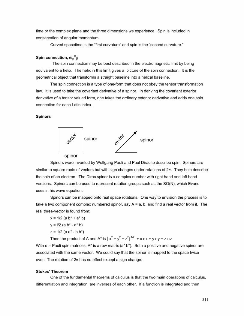
311

time or the complex plane and the three dimensions we experience. Spin is included in

conservation of angular momentum.

Curved spacetime is the “first curvature” and spin is the “second curvature.”

Spin connection, ωµα

β The spin connection may be best described in the electromagnetic limit by being

equivalent to a helix. The helix in this limit gives a picture of the spin connection. It is the

geometrical object that transforms a straight baseline into a helical baseline.

The spin connection is a type of one-form that does not obey the tensor transformation

law. It is used to take the covariant derivative of a spinor. In deriving the covariant exterior

derivative of a tensor valued form, one takes the ordinary exterior derivative and adds one spin

connection for each Latin index.

Spinors

spinor

spinor

vecto

r

vecto

r

spinor

Spinors were invented by Wolfgang Pauli and Paul Dirac to describe spin. Spinors are

similar to square roots of vectors but with sign changes under rotations of 2π. They help describe

the spin of an electron. The Dirac spinor is a complex number with right hand and left hand

versions. Spinors can be used to represent rotation groups such as the SO(N), which Evans

uses in his wave equation.

Spinors can be mapped onto real space rotations. One way to envision the process is to

take a two component complex numbered spinor, say A = a, b, and find a real vector from it. The

real three-vector is found from:

x = 1/2 (a b* + a* b)

y = i/2 (a b* - a* b)

z = 1/2 (a a* - b b*)

Then the product of A and A* is ( x2 + y2 + z2) 1/2 + x σx + y σy + z σz

With σ = Pauli spin matrices, A* is a row matrix (a* b*). Both a positive and negative spinor are

associated with the same vector. We could say that the spinor is mapped to the space twice

over. The rotation of 2π has no effect except a sign change.

Stokes’ Theorem One of the fundamental theorems of calculus is that the two main operations of calculus,

differentiation and integration, are inverses of each other. If a function is integrated and then

312

differentiated, the original function is retrieved. As a result, one can compute integrals by using

an antiderivative of the function to be integrated.

If you add up all the little changes in a curve then you get the total of the curve. If you

then break the curve into little changes again, you could retrieve those.

Stokes’ theorem states that the fundamental theorem is true for higher dimensions and

on manifolds. Evans has developed a covariant version.

Strong Field The strong interaction. This holds quarks and gluons together to make protons and

neutrons. Strong interactions provide the nuclear binding force. This is gravitational in nature

and may ultimately be more fully explained by some antisymmetric parts of Evans’ equations

also.

The weak force (interaction, field) is electromagnetic. The force between electrically

charged particles and between neutral atoms forming molecules is an electromagnetic

interaction.

SU(2), SU(3) Special unitary groups. See Groups.

Symbols a acceleration

c speed of light in vacuum

ds distance

g acceleration due to gravity; gravitational field strength; metric tensor

h Planck's constant; h-bar is Dirac’s constant

i imaginary unit; Cartesian x-axis basis unit vector

j Cartesian y-axis basis unit vector

k Einstein’s constant; Cartesian z-axis basis unit vector

l length; angular momentum

m mass

p momentum; pressure

q metric vector

r radius; distance

t time

u four-velocity

v velocity

B magnetic flux density; magnetic field

E energy; electric field

F force

313

G Einstein tensor; universal constant of gravitation

H magnetic field strength

K kinetic energy (also Ek)

R curvature; Ricci tensor

T temperature; tangential vector; torsion, stress energy tensor

U potential energy

V potential voltage

α angular acceleration; fine structure constant

β v/c = velocity in terms of c

Γ Christoffel symbol

γ Einstein Lorentz-Fitzgerald contraction, gamma

∆ change, difference between two quantities

ε permittivity

η metric –1, 1, 1, 1

θ angular displacement

κ torsion constant

λ wavelength

µ mu

ν nu

π 3.14; ratio of circumference / diameter of a circle

ρ density

τ torque; proper time; torsion

ω angular velocity, spin connection

Σ sum Φ field strength

Ψ wavefunction

Symmetric tensor A symmetric tensor is defined as one for which Amn = Anm with Greek indices, typically mu

and nu, used when working in 4 dimensions. (Latin indices are used in 3 dimensions.)

The symmetric tensors will typically describe distances. The antisymmetric tensors will

describe spin - turning or twisting.

Symmetry See Groups and Rotations also.

A symmetrical equation, group of vectors, or object has a center point, axis line, or plane

of symmetry. A mirror image is symmetrical with respect to the reflected object. A symmetrical

operation results in the same or a mirror figure as the original. Reflection, translations, rotations

314

are such operations. The symmetry group for an object is the set of all the operations that leave

the figure the same.

Symmetries are the foundation for the various conservation laws. Certain characteristics

remain unchanged during physical processes. Symmetries are usually expressed in terms of

group theory. Symmetry is one of the fundamental mathematical components of the laws of

physics defining invariance.

Einstein’s special relativity established that the laws of electromagnetism are the same in

any inertial reference frame – one that is not undergoing acceleration or in a gravitational field.

This can be described as a symmetry group – in mathematics, the Poincaré group.

General relativity extended theory to reference frames that are accelerating or

experiencing gravitational forces. All laws of nature, including electrodynamics and optics, are

field laws that are mapped in curved spacetime. A field can be reshaped without losing the

relationships within it. The Einstein group defines the symmetry in general relativity. Both are Lie

(pronounced lee) groups in mathematics. Tensors reshape vectors in different reference frames..

The invariant distance ds (not ds2) establishes the covariance of the laws of nature. One

takes the square root of ds2 using spinor forms. The Dirac equation does this by factorizing the

Klein-Gordon equation. Spin showed ramifications - extra degrees of freedom - and can be seen

in Evans as related to torsion. Quaternians can also be used to define the Riemannian metric.

The 4-vector quaternion fields are like the second-rank, symmetric tensor fields of the metric of

the spacetime.

Symmetry Operations or Transformations Rotations.

A spherical system -sphere, cylinder, or circle - can be rotated about any axis that passes

through its center. After a rotation the appearance of the system is unchanged. There is no

smallest change allowed. An infinitesimal rotation can be made and for this reason the symmetry

is continuous. (Evans does show us that h, Planck’s constant, and h bar, Dirac’s constant, do

Continuous Rotation of a Circle

Regardless of the amount of rotation, the circle isthe same after the operation.

315

establish minimum rotations in physics, but mathematics allows smaller changes.)

Discrete symmetries require unit steps. The rotation of a triangle is an example. Only

complete steps of 1/3 x 360º = 120º can occur to maintain symmetry. The operation either

happens in a distinct step or it doesn't happen at all.

Reflections or Parity Symmetry

The flip of the triangle is a reflection. A mirror reflects any object held up to it. Reflection

in time is time reversal symmetry.

The symmetry operations form an algebra called a symmetry group or simply group. The

mathematical definition of a group includes rules: Closure: the product of any two elements or

the square of an element yields another element in the set. Identity Element: the unitary

operation exists for each element so that one times R = R. Unique inverse element: each

element has an inverse so that R x R-1 = R-1 x R = 1. Association: R1 x (R2 x R3) = (R1 x R2) x R3.

Commutativity: . That is R1 x R2 = R2 x R1. Group multiplication does not have to be

commutative. A commutative group is Abelian (i.e., AB = BA for all elements A and B). The

equilateral triangle group is non-commutative, that is non-Abelian. The real universe is non-

Abelian. If non-Abelian then AB-BA has a value, otherwise AB-BA = 0.

The continuous group of all rotations in three dimensions - symmetry group of a sphere -

is SO(3). It governs the physics of angular momentum and spin. The symmetry of a sphere in N-

dimensions is called SO(N). SU(N) is the symmetry of the complex number unit sphere.

Translations.

Movement is a translation in space and time. If an object is moved from one place to

another, it’s shape is unchanged. Spatial translations are invariant. All relativistic equations in

physics are invariant under translations in space and time. The defining symmetry principle of

Rotation and reflection of a triangle

The rotation or reflection must be discrete for thetriangle to appear the same.

a

b

c

a bc120 degreerotation tothe right

a

b c

a

b c a

b

c

Reflectionabout the "c"

axis.

316

special relativity is invariance of physical laws. This is the Strong Equivalence Principle of

Einstein.

The term “proper time” is used to denote time as measured by an observer or clock within

a given reference frame. It is invariant. The symbol tau, τ, is used for proper time.

Charge Conjugation.

Particle-antiparticle symmetry is called charge conjugation. A discrete symmetry of

replacing all particles by anti-particles in any given reaction is called C. It is a necessary

condition in quantum mechanics that the combined operations of CPT must be an exact

symmetry. Experiments with neutral K-mesons indicate the violation of T-symmetry. T must be

violated when CP is violated in such a way as to make CPT conserved. CPT is expected to be

an exact symmetry. The violation of T means that there is fundamental information that defines a

preferred direction of time.

A particle's wave function can be changed to that of its antiparticle by applying CPT

operation: charge conjugation, parity, and time reversal operations. This leaves the momentum

unchanged.

C(e) = -e.

Time reversal invariance is not a symmetry law.

Strong interacting particles (like protons, neutrons, pi-mesons) are members of the

symmetry group, SU(3). One of the representations of SU(3) has eight components represented

as an irreducible 8 x 8 matrix. The eight spin-0 mesons fit into one matix; the eight spin-1/2

baryons into another matrix. The SU(3) symmetry is not exact, but the pattern exists.

Given that x2 + y2 + z2 = 1, then the set of linear maps from (x1, y1, z1) to (x2, y2, z2) so

that x22 + y2

2 + z22 also = 1 defines the symmetry group O(3). O(3) is the spherical symmetry

group used by Evans in electrodynamics.

The group of rotations on the complex numbers is the one-dimensional unitary group

U(1). O(2) is equivalent and acts on 2-dimensional vectors. Complex numbers can represent 2-d

vectors.

A map between two groups which keeps the identity and the group operation is called a

homomorphism. If a homomorphism has an inverse which is also a homomorphism, then it is an

isomorphism. Two groups which are isomorphic to each other are considered to be "the same"

when viewed as abstract groups. For example, the group of rotations of a triangle is a cyclic

group

Symmetry building of the field equations A new phenomenon may be indicated by the Evans equations. This is the inverse to

spontaneous symmetry breaking, for example from SU(2) x U(1) to U(1) = SO(2). As of this

writing there is indication that the B(3) field could be a consequence of "symmetry restoring" or

symmetry building. Evans has found that O(3) describes electrodynamics. (It could be that

317

SO(3) is the correct group for electrodynamics.) The subtleties involve preserving motion with or

without reflections and which group is more physical.

The highest symmetry is that of the unified field theory using the Einstein group.

Next is O(3) electrodynamics which is intermediate between Maxwell-Heaviside U(1).

The gravitational and electromagnetic fields are decoupled in O(3). It has higher symmetry than

U(1) electrodynamics.

Symmetry - Noether's Theorem In 1905, the mathematician Emmy Noether proved a theorem showing that for every

continuous symmetry of the laws of physics, there must exist a conservation law and for every

conservation law, there must exist a continuous symmetry.

Rotational symmetry is the law of conservation of angular momentum.

Mirror symmetry (Parity) or particle-antiparticle symmetry is charge conjugation.

Time reversal symmetry during translation is conservation of momentum. Translation symmetry

is conservation of momentum. In collisions, the momentum of the resulting particles is equal to

that of the initial particles.

Time translation symmetry is conservation of energy. As an object moves from time

space to time space, existence continues.

All of the individual conservation laws amount to conservation of existence. Nothing is

created or destroyed; but it can change aspects.

Evans has given us a new conservation law – conservation of curvature. That curvature

can be the first kind, Riemann curvature, or the second kind, torsion.

Tµν The stress energy tensor or energy-momentum tensor. It describes everything about the

energy of a particle or system. It contains the energy density, stress, pressure, and mass. In

Evans it must also be defined by the energy within the torsion.

T is the stress energy tensor which is the total energy density. It is the source of the

fields of relativity. All stress, pressure, velocity, mass, energy are part of T. And all the

components of T are the source of a gravitational field. T00 defines the energy density and Ti is

the momentum density. In a co-moving reference frame of SR, T = p, the momentum. T is

symmetric, that means that Tαβ = Tβα

T is used to define the curvature or compression parameters of the space due to energy

density.

318

Tangent spaces and bundles The tangent space is the real vector space of tangent vectors at each point of a manifold

or spacetime. The bundle is the collection of all the vectors.

The tangent space in GR is physical, the fiber bindle space in gauge theory has

heretofore been considered an abstract Yang Mills space. Evans’ shows that the tangent bundle

is the vector space of QT.

Tensors A tensor is a geometrical object which describes scalars or vectors, and linear operators

independent of any chosen frame of reference.

A tensor is a function which takes one or more vectors and calculates a real number

which will be the same in any reference frame. Knowing the real number, a scalar, and the

formula which found it allows us to move from reference frame to reference frame or from one

part of a curved space to another part.

Tensors are simply formulas or math machines. Plug in some numbers, vectors or 1-

forms and out comes a number or another vector or 1-form.

Tensors are linear, meaning they can be added or multiplied like real numbers. It gives

the same number regardless of reference frame – high velocity or dense gravitational field.

Components in a reference frame are the values of the function when its arguments are

the basis vectors, eα, of the reference frame. Components are frame dependent since basis

vectors are frame dependent. A rod is 1 meter long in frame A, but it will shrink in a high energy

The tangent space, acollection of all the

vectors and identifyingproperties of the point

on the manifold.

Point on the manifold.

The space or manifoldin our universe.

Tangent space

The tangent space is an infinitenumber of vector fields used as

needed to describe the point in thereal space.

319

density energy frame as viewed from a low energy density reference. When the entire reference

frame A changes, the components will be different in different reference frames – it is the tensor

which is invariant.

The number of dimensions of space are indicated by number of indices.

Rank is indicated by the number of different indices.

g or gµν is the metric tensor.

Gµν = Rµν – ½ gµν R is the Einstein tensor; sometimes called “Einstein.” Note bold face

letters used by some authors. Evans uses regular print which is the more modern format.

R is the scalar curvature. Rµν is the Ricci curvature tensor. It is the only contraction of

Riemann and it is symmetric. The Ricci curvature controls the growth rate of the volume of a

space.

Rµν is the Riemann tensor

Tµν is the stress energy tensor.

A tensor is symmetric if f( Aur

, Bur

) = f( Bur

, Aur

). Their components also obey fαβ = fβα. A tensor

is antisymmetric if f( Aur

, Bur

) = - f( Bur

, Aur

). Their components obey fαβ = - fβα.

Spinor space is antisymmetric.

A tensor of type M

N

is a linear function of M one-forms and N vectors onto the real

numbers. Rank is indicated by the number of different indices, M+N above.

Zero rank tensors are scalars.

First rank tensors are vectors.

Gµν is a second rank tensor.

If a tensor’s components vanish (go to zero) in one coordinate system, they will do so in

all coordinate systems.

Evaluation of a tensor, say Rσαγβ, involves partial differentials in all four dimensions.

Tensor contraction A form of dot product for tensors. Tensors with different indices are set equal to each

other and then summed. It is the operation of a 1-form on a vector.

Contraction is reduction in number of indices by applying a one form to a vector, or by

summing over repeated indices of mixed tensors. For example, if a one form operates on a

vector, the result gives the number of times they cross each other. It defines a point on each of

the one form’s planes.

Tensor Field Tensors usually describe potential fields. The metric tensor gµν describes the

gravitational field. We change local coordinates translating them to generalize, and put them in

320

some other part of the field. For example, we can take the velocity of a particle far from a black

hole and calculate a new velocity near the horizon.

Tensor product ⊗

Product of two tensors is another tensor. Also called the outer product.

Distinguished between wedge product and the inner or dot product. The inner product

produces a scalar arc length. It is the Pythagorean hypotenuse in four dimensions. I a b I I c d I

= ac + bd. Wedge product is defined as I a b I ∧ I c d I = ac - bd.

Tensor space A vector space of the products between vector fields and dual vector fields V* composed

of one forms. A linear map can be found that maps the vectors to the space.

Tetrad (vielbein) See one-forms also.

A vielbein (German for many legs) is more general than tetrad and refers to any number

of dimensions. The term “tetrad” means a group of four vectors which are orthonormal to one

another. The tetrad defines the basis vectors for a space. The tetrad is a 4 x 4 matrix. See Basis

Vectors.

The advantages using the tetrad is that it allows spinors needed for the Dirac equation to

be developed in general relativity, and allows the development of the Maurer Cartan structure

relations.

In the Evans equations the fields are tetrads and the gravitational and gauge fields are

built from tetrads using differential geometry. Tensors were initially used in Riemann geometry to

describe curved space. Tetrads give an alternate but equivalent mathematical method of

describing general relativity. They are four reference vector fields, ea. With a = 0, 1, 2, and 3

such that g(ea,eb)=ηab. The tetrad has a linear map from an internal space bundle to the tangent

bundle and defines a metric on spacetime.

The tetrad formulation of GR is similar to a gauge theory and allows viewing GR in a

fuller sense with electromagnetism, the strong, and the weak fields explained in the same terms.

The tetrad is the frame field e = basis coordinates in the tangent bundle.

Outer Productq0 q0 q1 q2 q3 = q0q0 q0q1 q0q2 q0q3

q1 q1q0 q1q1 q1q2 q1q3

q2 q2q0 q2q1 q2q2 q2q3

q3 q3q0 q3q1 q3q2 q3q3

321

A spin structure is locally a tetrad where it has a local Lorentz index and spacetime index.

A spin structure contains more information than a metric structure.

The tetrad relates orthonormal bases to coordinate bases.

The torsion tensor is defined for a connection on the tangent bundle. It is the covariant

exterior derivative of the tetrad.

Given two topological spaces, A and C, a fiber bundle is a continuous map from one to

the other. C is like a projection. For example if A is a human body and C is a shadow, then the

mathematical lines connecting them is B and would be the fiber bundle. The ground would be

another topological space, C. The space C could be a vector space if the shadow is a vector

bundle. The bundle is the mapping. The tetrad is a matrix at each point that describes the

connections.

The tetrad is the eigenfunction for the O(3), SU(2) and SU(3) representations.

The tangent space to a manifold is connected by a bundle. The tetrad provides the

connections. Those connections could be quite complex. In the case of the shadow, the

formulas describing the angles are contained in the tetrad.

Gauge theory uses fiber bundles. Spinor bundles are more easily described by the tetrad

than by the more traditional metric tensors.

It is important to know that the tetrad is a group of four vectors that are orthonormal to

one another. The tetrad defines the curvature of the space in certain terms. By orthonormal we

mean that they are at right angles to one another with respect to the curved space. They are not

perpendicular since the space is not Euclidean. These vectors are both orthogonal and

normalized to unit magnitude allowing the basis vectors to be used. Two vectors are orthogonal if

their dot product equals 0. They are not necessarily at right angles to each other in flat space.

The four dimensional space is curved and twisted and the vectors must align.

The tetrad is defined by:

Va = qaµ Vµ

Where Va is a four-vector in the orthonormal space and Vµ is a four-vector in the base manifold.

Then qaµ is a 4 x 4 matrix whose independent components correspond to the irreducible

representations of the Einstein group.

Each component of the matrix is an eigen-function of the Evans wave equation:

µ( + kT)q = 0a

322

The gravitational field is the tetrad matrix itself.

The electromagnetic potential field is the matrix:

Aaµ = A(0) qa

µ

where A(0) is voltage.

In terms of basis vectors, the inner product can be expressed as g (ê(a), ê(b)) ηab where g (

, ) is the metric tensor. And ê(µ) = ∂µ where µ indicates 0, 1, 2, 3, the dimensions of spacetime

base manifold. This indicates the curvature at the point.

ê(µ) = qaµ ê(a)

This is most important in the mathematical development of the unified field theory, but a

full explanation is impossible here. It is shown for completeness. The tetrad refers to a 4-

dimensional basis-dependent index notation.57

In defining the tetrad (Va = qaµ Vµ ) two contravariant vectors are used and where Va is

any contravariant vector in the orthonormal basis indexed a and Vµ is any contravariant vector in

the base manifold, µ.

It is possible to use both a contravariant or a covariant vector both in the space of ‘a’ and

in the space of µ. Carroll is an excellent source of information on the tetrad and is essential

preliminary reading for Evans’ works. See references.

Using the definition of qaµ

, the tetrad in Va = qaµ

Vµ, V could represent position vectors, x,

and the tetrad would be xa = qaµ xµ.

The tetrad could be defined in terms of Pauli or Dirac matrices or spinors, or Lorentz

transformations.

57 Vielbein refers to any dimensional approach with triad the 3-dimensional

version and pentad the 5-dimension. Vierbein is synonymous with tetrad.

µq =a

0q0

1q0

2q0

3q0

0q1

1q1

2q1

3q1

0q2

1q2

2q2

3q2

0q3

1q3

2q3

3q3

General expression for the tetrad matrix

323

The tetrad mixes two vector fields, straightens or absorbs the non-linearities, and

properly relates them to each other.

qaµ can be defined in terms of a scalar, vector, Pauli two-spinors, or Pauli or Dirac

matrices. It can also be a generalization between Lorentz transformation to general relativity or a

generally covariant transformation between gauge fields.

When metric vectors are used, the tetrad is defined:

qa = qaµ qµ

and the symmetric metric is defined by a dot product of tetrads:

qµν (s) = qa

µ qbν ηab

where ηab is the metric (-1, 1, 1, 1)

In the most condensed notation of differential geometry, the Greek subscript indices

representing the base manifold (non-Euclidean spacetime) are not used (because they are

always the same on both sides of an equation of differential geometry and become redundant).

Here we keep them for basic clarity.

The tetrad is a vector valued one form, and can be thought of as a scalar valued one

form (a four vector, with additional labels). It is the mapping. If a contravariant 4-vector Va is

defined in the tangent (representation) space and another, Vµ, is defined in the non-Euclidean

space (base manifold) of general relativity, then the tetrad is the matrix that relates these two

frames:

Va = qaµVµ

where the superscript a represents the three space indices and one time index and µ represents

the four dimensions of the base manifold of our spacetime.

The Evans wave equation with tetrad as eigenfunction states:

DνDνqaµ = ( + kT) qa

µ = 0

Tetrad postulate Cartan’s concept that the values in the curved space of our universe can be connected

and calculated in the flat mathematical index space. Also called “moving frames.”

The tetrad postulate is: ∇µ eaµ = 0.

Theory of everything – Unified Field Theory A theory that unifies the four fundamental forces – gravity, strong nuclear force, weak

force and electromagnetic force. Quantum gravity is one such attempt. General relativity and

quantum chromodynamics can be brought together by a unified theory. So far GUT’s or Grand

Unified Theories have not brought gravity into consideration. Evans’ equations unify physics as

they are developed since gravity and electromagnetism are now shown to be two aspects of a

common geometric origin described by differential geometry.

324

Time The fourth dimension. In general relativity and Evans unified field theory it is treated as a

4th spatial dimension. In black holes the mathematics shows reversal of time and space

indicating that they are different aspects of the same basic thing. In Minkowski space, time and

space are combined into spacetime.

The use of c in many equations indicates that time is being converted to spatial distance.

For example ct in the invariant distance in special relativity or 1/c in various wave equations or the

d’Alembertian.

c is the velocity of time.

Time becomes an operator in the quantum sector of Evans equations.

Torsion Torsion is the rate of change of an osculating plane. It is positive for a right hand curve

and negative for a left hand curve. The radius of torsion is φ or σ = 1/τ

If referring to a group, then the torsion is the set of numbers that describe the torsion of

the individual elements.

Cartan torsion is the anti-symmetric parts of a Christoffel symbol.

Also referred to as “dislocation density” or the “second curvature” in some texts where

“first curvature” is our standard definition of curvature in three planes. Torsion is then curvature in

the 4th dimension.

Torsion tensor

The torsion of a curve is a measurement how much the curve is turning, or of twist. The

torsion tensor measures the torque of one 4-vector field with respect to another 4-vector field.

Torsion

325

Torsion describes a connection in spacetime which is antisymmetric. The torsion tensor

is a connection on the tangent bundle and can be thought of as the covariant exterior derivative of

the tetrad.

Trace Sum of the diagonal terms of a matrix.

Unified Field Equations The Evans equations are the unified field equations. He has developed homogeneous

and inhomogeneous, equations. They are reduced to the Einstein and Maxwell Heaviside limiting

forms and they become the field equations of O(3) electrodynamics. The equations can derive all

the known equations of quantum mechanics, general relativity, and Newtonian mechanics.

Unit vectors See Basis vector.

Vacuum Vacuum can be used several ways. It is the spacetime of quantum mechanics and

experiences polarization and has content. We can see more clearly from Evans’ work that

curvature and torsion are everywhere. Since curvature and torsion can produce particles, the

vacuum is more substantially understood due to Evans clear explanation of electromagnetism as

twisting or spinning spacetime.

Vacuum has been described erroneously in some texts as a total absence of anything.

This could be a matter of definition.

The stochastic granular school sees the vacuum as a tenuous something. Given that

quarks can be pulled out of the vacuum, it has at least a potential and that makes it something. It

may be that the electromagnetic fields of the universe are the only thing present in the vacuum

and the vacuum polarization is field based.

In the older viewpoint, given that an electron’s location approaches infinite distance (r →

∞) from the center of every atom at a low probability (IΨI2 → 0), then the vacuum is full of

fleeting matter and electromagnetics. In Evans viewpoint, curvature and torsion in one region

extend into others.

False vacuum is hypothesized to have a positive energy and negative pressure and to be

the force that drove the expansionary period of the universe. This is purely theoretical.

Void is the real nothing outside the universe and maybe exposed inside the ring

singularity of a Kerr black hole. That void is as close as the space in front of your face. The

vacuum interface to the void is everywhere in 4d space.

Evans gives us a definition of quantum vacuum equaling Minkowski spacetime.

326

Vacuum is very low mass density spacetime. It can be severely curved or torqued near a

black hole.

Vectors Vectors are numbers with magnitude and direction. The vector is sometimes indicated

as a bold letter or with an above it. In order to be added or multiplied together, they must have

the same units. A negative of a vector has the same magnitude but is opposite in sign which

indicates direction.

The vector is a geometric object. It does not need a reference frame to exist. It can be

changed from one reference frame to another by math operations.

The velocity of a particle is a vector tangent to the path in spacetime that the particle

follows. This is tangent to the 4-dimensional path.

Components of a vector are the axes of a rectangular coordinate system.

Tensors and vectors are similar in this respect.

The expressions are often: x0, x1, x2, and x3. Thus xα means x0, x1, x2, and x3.

At each point in spacetime there are a variety of vectors describing the curvature, torsion,

mass, and energy.

The 4 velocity of a particle is a vector tangent to the path in spacetime that the particle

follows. This is tangent to the 4-dimensional path.

Y

X

Vector

327

Vector Field

A map which gives a real or complex vector for each point on a space. The bundle is all

the vectors of the entire space. A vector field is a section of the entire bundle. The vectors exist

in the mathematical tangent space. The information about each vector is within the field. The

number of dimensions is defined and the bundle could be infinite. Typically, the tangent space to

our real four dimensional space has all the mathematical information about the mass, curvature,

etc.

Vector space A set of vectors can be defined for which addition and multiplication produce real or

complex scalars. The vectors are placed in a vector space and can be moved among reference

frames by tensors.

Vielbein See Tetrad.

Wave equation Wave equations are partial differential equations:

∇ 2ψ = 1 ∂2ψ v2 ∂t2

V xo,yo = (ax + bi)

Each vectorhas

informationattached:

A vector fieldand two

integral curves

328

∇ 2 is the Laplacian and ψ is a probability. 2 is the d'Alembertian, the 4-dimensional

version of the Laplacian.

Wave or Quantum Mechanics Study of basic physics starting with the Planck quantum hypothesis. The dual nature of

existence as a wave and particle is recognized as a foundation concept.

Wave number k or = 1/ or 2

The rest wave number is defined by Evans as 0 = 1/0 = IR0I1/2

See http://scienceworld.wolfram.com/physics/Wavenumber.html

The de Broglie wavenumber is k = 2πρ/h = π/ћ

Wave velocity v = λ f = (2π / k) (ω/2π) = ω / k

Weak field Low curvature and torsion. Low mass, energy, velocity, electrical potential, or

gravitational field.

Wedge or exterior product The wedge product is a vector product defined in a vector space. It is the 4 or more

dimensional version of the cross product.

x,tx

t

A sine wave is a function of x and t in two dimensions.

329

REFERENCES To Do

Advances in Physical Chemistry,………

The Enigmatic Photon, M. Evans and J. Vigier, Kluwer Academic Publishers,

Dordrecht, 2002, (Paperback, five volumes).

Generally Covariant Unified Field Theory – The Geometrization of Physics, M. W.

Evans, Kluwer Dordrecht, van der Merwe Series, 2005.

The Geometry of Physics, An Introduction, Theodore Frankel, Cambridge

University Press, 1997.

Lecture Notes on General Relativity, Sean M. Carroll, Institute for Theoretical

Physics, University of California, Santa Barbara, CA, December 1997, www.arXiv:gr-

qc/9712019 v1 3 Dec 1997.

The Meaning of Relativity, Albert Einstein, Princeton University Press, 1921,

1945.

Quantum Mechanics: Symmetries, Walter Greiner and Berndt Mueller, Springer,

New York, 1994.

Ryder ……….

Towards a Nonlinear Quantum Physics, J.R. Croca, World Scientific Pub.

Singapore ; River Edge, NJ, 2003. "