
The EU Electricity Network Codesflorenceonlineschool.eui.eu/wp-content/uploads/2016/09/FSR-NC... ·...
96
I The EU Electricity Network Codes Course text for the Florence School of Regulation online course By Leonardo Meeus and Tim Schittekatte October 2017
Transcript of The EU Electricity Network Codesflorenceonlineschool.eui.eu/wp-content/uploads/2016/09/FSR-NC... ·...

I
The EU Electricity Network Codes
Course text for the Florence School of Regulation online course
By Leonardo Meeus and Tim Schittekatte
October 2017
II
Contents Abbreviations ....................................................................................................................................... VIII
Disclaimer & invitation to contribute ...................................................................................................... X
Acknowledgements ................................................................................................................................ XI
Suggested reading guideline: native, advocate and master ................................................................. XII
1. Introduction ......................................................................................................................................... 1
The network codes and guidelines ................................................................................................ 1
1.1.1 Three groups of network codes.............................................................................................. 1
1.1.2 Network codes versus guidelines ........................................................................................... 1
1.1.3 Focus of this course text (for now) ......................................................................................... 2
Why do we have so many electricity markets? ............................................................................. 3
Electricity market sequence .......................................................................................................... 3
2. The link between markets and grids in the EU: key concepts ............................................................. 6
Local: Bidding Zones (market) and Control Areas (grid) ............................................................... 6
Regional: Capacity Calculation Regions (market) and Regional Security Coordinators (grid &
market) ................................................................................................................................................ 8
Balancing Areas: in between markets and grids ........................................................................... 9
3. Forward markets ............................................................................................................................... 12
Forward energy markets ............................................................................................................. 12
Integration of forward markets: long-term (cross-zonal) transmission (capacity) rights ........... 13
3.2.1 Allocation: Harmonised rules and a single European platform............................................ 13
3.2.2 Calculation of future cross-zonal transmission capacity ...................................................... 14
3.2.3 Products and pricing ............................................................................................................. 14
3.2.4 Firmness ............................................................................................................................... 17
4. Establishing national day-ahead and intraday markets .................................................................... 19
Nominated Electricity Market Operators (NEMOs) .................................................................... 20
4.1.1 Scope and tasks .................................................................................................................... 20
4.1.2 Cost-of-service regulated versus merchant ......................................................................... 21
The day-ahead market (DAM) ..................................................................................................... 22
4.2.1 Bid formats: simple, block and complex bids ....................................................................... 23
4.2.2 Temporal granularity ............................................................................................................ 24
4.2.3 Maximum and minimum clearing prices .............................................................................. 25
The intraday market (IDM) .......................................................................................................... 25
4.3.1 Continuous trading versus auctions ..................................................................................... 26
III
4.3.2 Liquidity in the IDM .............................................................................................................. 29
4.3.3 IDM gate closure: the gap between trading and real-time operation ................................. 31
Matching markets with grids: redispatch and countertrading ................................................... 32
5. Integrating day-ahead and intraday markets .................................................................................... 34
Day-ahead market integration .................................................................................................... 34
5.1.1 Explicit vs. implicit allocation of transmission capacity........................................................ 36
5.1.2 Cross-zonal capacity calculation: issues and approaches .................................................... 38
Intraday market integration ........................................................................................................ 44
5.2.1 Integration with continuous trading .................................................................................... 45
5.2.2 Continuous trading complemented with (regional) intraday auctions ................................ 46
6. Establishing national balancing markets ........................................................................................... 47
Reserve sizing .............................................................................................................................. 49
The balancing markets: capacity and energy .............................................................................. 51
6.2.1 Balancing capacity market and its key market design parameters ...................................... 52
6.2.2 Balancing energy market and its key market design parameters ........................................ 54
Imbalance settlement mechanism .............................................................................................. 57
6.3.1 Pricing rule for imbalance charges ....................................................................................... 58
6.3.2 Balancing capacity cost allocation ........................................................................................ 60
6.3.3 Single vs. dual imbalance pricing .......................................................................................... 62
The activation of balancing energy: two approaches ................................................................. 65
7. Integrating balancing markets ........................................................................................................... 69
How far should harmonisation go to allow for integration? ....................................................... 70
Inter-TSO cooperation in balancing ............................................................................................. 71
7.2.1 Less and cheaper balancing energy: imbalance netting and the exchange of balancing energy
....................................................................................................................................................... 72
7.2.2 More efficient reserve procurement and sizing: exchange of reserves and reserves sharing
....................................................................................................................................................... 74
IV
List of Figures Figure 1: Status of the implementation phase of the network codes in May 2017 (ENTSO-E, 2017) .... 2
Figure 2: The sequence of electricity markets in the EU and related network codes and guidelines
(Adapted from FSR (2014)) ...................................................................................................................... 4
Figure 3: Left-Bidding zones in 2017 (Ofgem, 2014). Right- Control areas in Germany (Wikiwand, 2017)
................................................................................................................................................................. 7
Figure 4: Left- Proposal of ENTSO-E (2015a) for the Capacity Calculation Regions (ENTSO-E, 2015b).
Right – An overview of the Regional Security Coordinators in Europe (ENTSO-E, 2017a)...................... 8
Figure 5: Left- FCA/CACM (markets) vs. EBGL (balancing) vs SOGL (system operation) terminology to
denote geographical areas (adapted from ENTSO-E, 2014b). Right- the different synchronous areas in
Europe (ENTSO-E, 2017k) ...................................................................................................................... 10
Figure 6: Ratio of traded volume in forward markets over 2014 consumption (ACER/CEER, 2016) .... 13
Figure 7: Energy delivery scenarios to illustrate the difference between obligations and options, based
on PJM (2011) ........................................................................................................................................ 15
Figure 8: The hourly DA and ID market trading volume as share of the hourly consumption for France
and Germany (Brijs et al., 2017) ............................................................................................................ 19
Figure 9: Facts and figures of NEMOs in the EU (excl. Cyprus and Malta). Based on ACER (2015a) .... 20
Figure 10: Example of the clearing of an aggregated demand (blue) and supply curve (red) for one hour
of the DAM in Romania on 24/01/2011 (Pérez-Arriaga, 2013) ............................................................. 22
Figure 11: Trading process from the DAM to the IDM gate closure in Germany by EPEX (Neuhoff et al.,
2016b) ................................................................................................................................................... 26
Figure 12: Intraday markets in selected European countries with 2012 data (Hagemann and Weber,
2015) ...................................................................................................................................................... 30
Figure 13: State-of-play in Price Coupling of Regions (PCR) as of February 2017 (ENTSO-E, 2017e) ... 35
Figure 14: DAM price convergence from 2008-2015 (ACER/CEER, 2016) ............................................. 36
Figure 15: Zonal pricing and optimal cross-zonal allocation (FSR, 2014) ............................................. 37
Figure 16: Explicit cross-zonal allocation: use of net daily capacities on the French-Spanish
interconnector compared with hourly DAM price differences, data of 2012 (FSR, 2014) ................... 37
Figure 17: Implicit cross-zonal allocation : use of net daily capacities on the France-Belgium
interconnector compared with hourly price differences, data of 2012 (FSR, 2014) ............................ 38
Figure 18: Scheduled flows (black), transit lows (white-left) and loop flows (white-right) (Schavemaker
and Beune, 2013) .................................................................................................................................. 39
Figure 19: Grid model under the ATC approach (left) and flow domain (right) (Van den Bergh et al.,
2016) ...................................................................................................................................................... 40
Figure 20: Grid model under FB approach (left) and flow domain (Van den Bergh et al., 2016) ......... 41
Figure 21: State-of-play of XBID as of February 2017 (ENTSO-E, 2017e) .............................................. 45
Figure 22: A frequency drop and the reserve activation structure (Elia and TenneT, 2014) ................ 48
Figure 23: The four building blocks of the balancing mechanism, financial and physical relationships
and relevant network codes (adapted from Hirth and Ziegenhagen, 2015) ........................................ 48
Figure 24: Duration curves of the net regulated volume (NRV) in France and Germany for 2012-2015
(Brijs et al., 2017)................................................................................................................................... 55
Figure 25: Overall cost of balancing (energy plus capacity) and imbalance charges over the electricity
consumption per country in 2015 (ACER/CEER, 2016) ......................................................................... 60

V
Figure 26: Classification of European balancing markets based on activation strategy in balancing
energy and BRP incentives (Haberg and Doorman, 2016). Additionally, Portugal and Spain are identified
as proactive by the Pentalateral Energy Forum (2016) ......................................................................... 66
Figure 27: Overview of the balancing pilot projects (ENTSO-E, 2017h) ................................................ 69
Figure 28: Illustration of the efficiency gains with a common merit order list for the activation of
balancing energy under no congestion. ‘p’: price, ‘q’: quantity and ‘d’: demand (Elia et al., 2013). ... 73

VI
List of Tables Table 1: Terms for reserve products (based on E-Bridge consulting GmbH and IAEW, 2014) ............. 47
Table 2: Financial flows between TSOs and BRPs for imbalances (EBGL, Art. 55(1)) ............................ 58
Table 3: Summary of the three approaches for cross-zonal capacity allocation for the exchange of
balancing capacity or sharing of reserves. ............................................................................................ 77
VII
List of Boxes
Box 1: Financial transmission rights (FTR): obligations vs. options, illustrative exercise. ..................... 15
Box 2: The Nordic approach to long-term transmission rights (based on Spodniak et al. (2017)) ....... 16
Box 3: The optimal auction clearing rule – Marginal (or uniform) pricing vs. pay-as-bid ..................... 27
Box 4: The participation of resources connected to the distribution grid in balancing markets and the
power of the DSO .................................................................................................................................. 51
Box 5: The scoring rule for balancing markets ...................................................................................... 53
Box 6: The settlement rule in balancing energy markets – specific technical difficulties and
implementations in the Netherlands, Belgium and Spain .................................................................... 56
Box 7: The “Price Average Reference Volume (PAR)” approach in the UK (based on ACER/CEER (2016)
Littlechild (2015, 2007) and Ofgem (2015)) .......................................................................................... 59
Box 8: Self-dispatch versus central dispatch models ............................................................................ 67
Box 9: Two regional balancing initiatives – TERRE and EXPLORE .......................................................... 70
Box 10: ‘The German Paradox’ – more renewables but less and cheaper reserves? ........................... 72
VIII
Abbreviations
4MMC: 4M Market Coupling
AC: Alternating Current
ACER: Agency for the Cooperation of Energy Regulators
aFRR: Automatic Frequency Restoration Reserve
ATC: Available Transfer Capacity
AM: Availability Margin
BM: Balancing Market
BRP: Balance Responsible Party
BSP: Balancing Service Provider
CACM: Capacity Allocation and Congestion Management Guideline
CE: Central Europe
CEE: Central-East Europe
CEER: Council of European Energy Regulators
CCR: Capacity Calculation Region
CNE: Critical Network Element
CoBA: Coordinated Balancing Area
CWE: Central-West Europe
DA(M): Day-ahead (market)
DC: Direct Current
DR: Demand Response
DSO: Distribution System Operator
EBGL: Electricity Balancing guideline
ENTSO-E: European Network of Transmission System Operators for Electricity
EU: European Union
EUPHEMIA: EU Pan-European Hybrid Electricity Market Integration Algorithm
FRCE: Frequency Restoration Control Error
FB(MC): Flow-Based (Market Coupling)
FCA: Forward Capacity Allocation Guideline
FCP: Frequency Containment Process
FCR: Frequency Containment Reserve
FRP: Frequency Restoration Process
FRR: Frequency Restoration Reserve
FTR: Financial Transmission Right
GCC: Grid Control Cooperation
GCT: Gate Closure Time
HVAC: High Voltage Alternating Current
HVDC: High Voltage Direct Current
Hz: Hertz

IX
ID(M): Intraday (market)
ISP: Imbalance Settlement Period
IEM: Internal Energy Market
IGCC: International Grid Control Cooperation
JAO: Joint Allocation Office
LFC: Load-Frequency Control
LOLP: Loss of Load Probability
MCO: Market Coupling Operator
mFRR: Manual Frequency Restoration Reserve
MO: Market Operator
MRC: Multi-Regional Coupling
MS: Member State of the EU
MW: Mega Watt
MWh: Mega Watt Hour
NEMO: Nominated Electricity Market Operator
NRA: National Regulatory Agency
NRV: Net Regulated Volume
NTC: Net Transmission Capacity
ORDC: Operating Reserve Demand Curves
OTC: Over-The-Counter
PCR: Price Coupling of Regions
PTDF: Zonal Power Transfer Distribution Factor
PTR: Physical Transmission Right
RR: Replacement Reserve
RRP: Replacement Reserve Process
RSC: Regional Security Coordinators
RSCI: Regional Security Coordination Initiative
SEE: South-East Europe
SOGL: System Operations Guideline
TSO: Transmission System Operator
US: United States
VOLL: Value of Lost Load
vRES: variable Renewable Energy Sources (e.g. wind and solar)
XBID: Cross-Border Intraday Market Project

X
Disclaimer & invitation to contribute
This text has been written for the online course ‘’EU Electricity Network Codes’’ organised by the
Florence School of Regulation and directed by prof. Leonardo Meeus.
The first edition of this course is held in October-November 2017 and focuses on the market codes and
their interaction with the system operation codes. The next edition in October-November 2018 will also
include modules on the grid connection codes and the legal issues around network codes. This version
of the text is to support the first edition, and we will update the text for the next edition.
This text is a work in progress. Some topics are elaborated to a greater extent than others. We also
started to include different views on key issues; some are described in more detail than others. The
implementation of the network codes is an ongoing process, so this text will need to be updated
continuously. We invite you to read the text, and also to help us improve it.
You can contribute by adding comments and track changes here (link). Based on your feedback we will
develop the text into a book. Everybody that contributed will be thanked by name in the
acknowledgements.
Leonardo Meeus & Tim Schittekatte
In case you would like to refer to the current document, please it cite as:
Meeus, L. & Schittekatte, T. (2017). The EU Electricity Network Codes: Course text for the Florence
School of Regulation online course. Version of October 2017.

XI
Acknowledgements
We are very grateful for insights and remarks from Mathilde Lallemand, Athanasios Troupakis, Marco
Foresti, Alexander Dusolt, Anne de Geeter, Martin Roach, Samson Hadush, Nicolò Rossetto and Ross
Baldick.
Disclaimer: The authors are responsible for any errors or omissions.

XII
Suggested reading guideline: native, advocate and master
The course text is build up taken into account that this course is aimed at three types of participants
(native, advocate and master) with a distinct level of prior knowledge of the topic or objectives.
All participants are suggested to read Chapter 1 and Chapter 2. After, in Chapters 3-7 the paragraphs
addressed to advocate or master participants are marked as such. When not, -the default case- the text
is suggested to all participants.
Before starting the course, it is indispensable to read the introduction (Chapter 1) in which the different
network codes and their link with electricity markets are briefly described. Additionally, it is set out why
there is no one electricity market, but a sequence of electricity markets in place. Chapter 2, introducing
key concepts related to the network codes, is not directly linked to a particular week and will prove
useful throughout the whole course.
In the Table below an overview is given of the topic, relevant network codes and reading material per
learning week.
Topic Relevant network codes Reading material
Week 1 Establishing national wholesale markets
FCA, CACM 2.1 & 2.2 / Chapter 3 / Chapter 4 (excl. 4.4)
Week 2 Integrating national wholesale markets
CACM, SOGL 4.4 / Chapter 5
Week 3 Establishing national balancing markets
EBGL, SOGL 2.3 / Chapter 6
Week 4 Integrating national balancing markets
EBGL, SOGL Chapter 7
The Boxes spread throughout the course text are in most cases optional reading material1 and can help
to illustrate more abstract concepts.
1 Except for Box 4: The participation of resources connected to the distribution grid in balancing markets and the power of the DSO of which some points come back in the quiz of week 3.

1
1. Introduction
The network codes and guidelines
The development of network codes and guidelines has been identified as a crucial element to spur the
ongoing completion of the internal energy market in the Third Energy Package. More specifically,
Regulation (EC) 714/2009 sets out the areas in which network codes will be developed and a process
for developing them. These codes are a formalised detailed set of rules pushing for the harmonisation
of former more nationally oriented electricity markets and regulations. In 2017, after a 4-year lasting
co-creating process of ENTSO-E, ACER, the EC and many involved stakeholders from across the
electricity sector, the network codes have been developed. After the development of a network code,
the implementation phase can start.
1.1.1 Three groups of network codes
Eight network codes and guidelines came out of the co-creating process. Today, six of eight regulations
are entered into force. Two are validated by the Member States, but awaiting validation by European
Parliament and Council before being published in the Official Journal of the European Union as
commission regulation. Twenty days after publication, the commission regulation enters into force.
These eight regulations can be subdivided into three groups:
• The market codes: o The capacity allocation and congestion management guideline (CACM) – published on
25 July 2015 o The forward capacity allocation guidelines (FCA) – published on 27 September 2016 o The electricity balancing guideline (EBGL) – awaiting validation by the European
Parliament and Council, final version available from 16 March 2017
• The connection codes: o The network code on requirements for grid connection of generators (RfG NC) -
published on 14 April 2016 o The demand connection network code (DCC) – published on 18 August 2016 o The requirements for grid connection of high voltage direct current systems and direct
current-connected power park modules network code (HVDC NC) – published on 8 September 2016
• The operation codes: o The electricity transmission system operation guideline (SOGL) - published on 25
August 2017 o The electricity emergency and restoration network code (ER) - awaiting validation by
the European Parliament and Council, provisional final version available from 25 October 2016
1.1.2 Network codes versus guidelines
The eight regulations in which common rules for the electricity system and market are described, often
referred to as ‘’The network codes”, are actually not all network codes by definition. Four out of eight
are guidelines (CACM, FCA, EBGL and SO) and the other four are network codes (ER, RfG NC, DCC and
HVDC NC). All texts were initially planned to be network codes, and some became guidelines in the
development process. Below similarities and differences between network codes and guidelines are
listed.2
2 For more details, please consult Regulation (EC) 714/2009, in particular Article 6 and 18.
2
Similarities:
- The same value (both commission regulation and legally binding)
- Both are directly applicable
- The same adoption procedure (Comitology procedure)
Differences:
- Legal basis in the electricity regulation
- Development process
- Topics3
- Work to be done in the implementation phase
A significant difference between both is that guidelines included processes whereby a set of TSOs at
Pan-European or Regional level must develop a methodology submitted to the regulator for approval
after, in most cases, a public consultation. Network codes do not have such processes.
It can be argued that a network code is more detailed, while guidelines shift more tasks to the
implementation phase. The positive side of this is that guidelines allow for more flexibility in the
amendment process. This can prove helpful as the methodologies described in the guidelines could be
subjected to change as the sector evolves rapidly. On the other hand, shifting tasks to the
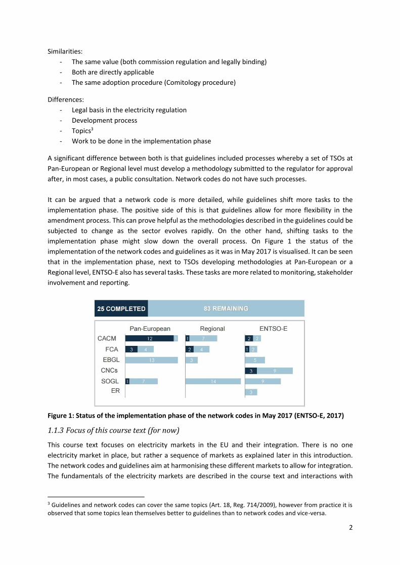
implementation phase might slow down the overall process. On Figure 1 the status of the
implementation of the network codes and guidelines as it was in May 2017 is visualised. It can be seen
that in the implementation phase, next to TSOs developing methodologies at Pan-European or a
Regional level, ENTSO-E also has several tasks. These tasks are more related to monitoring, stakeholder
involvement and reporting.
Figure 1: Status of the implementation phase of the network codes in May 2017 (ENTSO-E, 2017)
1.1.3 Focus of this course text (for now)
This course text focuses on electricity markets in the EU and their integration. There is no one
electricity market in place, but rather a sequence of markets as explained later in this introduction.
The network codes and guidelines aim at harmonising these different markets to allow for integration.
The fundamentals of the electricity markets are described in the course text and interactions with
3 Guidelines and network codes can cover the same topics (Art. 18, Reg. 714/2009), however from practice it is observed that some topics lean themselves better to guidelines than to network codes and vice-versa.

3
network codes and guidelines are highlighted.4 As this course talks about electricity markets, the most
relevant network codes are the market codes (CACM, FCA and EBGL). However, also the SOGL is of
importance, as markets and system operation cannot be fully decoupled.
Why do we have so many electricity markets?
Electricity markets do differ substantially from markets for copper, oil and grain. However, electricity
can be considered a commodity, just as copper, oil and grain are.5 The underlying reason for these
differences are the physical characteristics of electricity:
• Time: large volumes of electricity cannot be stored economically (yet). Therefore, electricity has a different cost and value over time.
• Location: electricity flows cannot be controlled6 easily, and transmission components should be operated under safe flow limits. If not, there is a risk of cascading failures and black-outs. Therefore, electricity has a different cost and value over space.
• Flexibility: demand can vary sharply over time, while most power stations can only change output slowly and can take many hours to start up. Also, power stations can fail suddenly. Demand and generation must match each other continuously if not there is a risk for a black-out. Therefore, the ability to change the generation/consumption of electricity after short notice has a value.
These three unique physical characteristics offer an explanation why there is not just one electricity
market. Electricity is not only energy in MWh. Transmission and flexibility are scarce resources and
should be priced accordingly. Therefore, electricity (energy, transmission, flexibility) is exchanged in
several markets until the delivery in real-time.
Electricity market sequence
Different markets allow putting a price on the “invisible” components of electricity and function as a
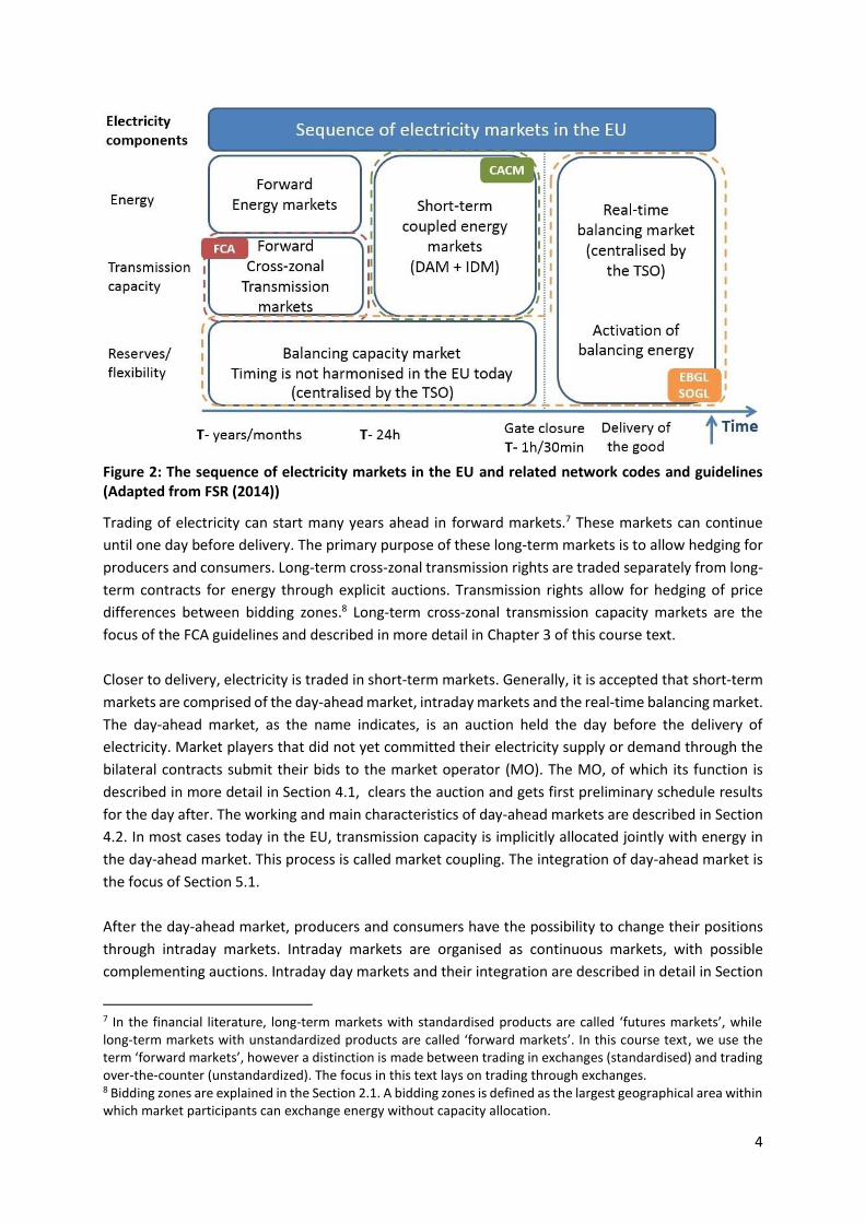
sequence. On Figure 2 the successive markets along the three electricity components are shown.
Additionally, the relevant guidelines are displayed per market. It should be noted that next to trading
through organised electricity markets (exchanges), energy can also be traded bilaterally over-the-
counter (OTC), in which market players (electricity generators, retailers, large consumers, and other
financial intermediaries) agree on a trade contract by directly interacting with each other. In this text,
electricity exchanges are the focus. Unlike bilateral contracts, products on exchanges are tradable,
implying transparent prices.
4 The course treats above all the text of the guidelines. The technical details of the methodologies, described in the guidelines and for which in most cases the development is ongoing, are in most cases out of scope. 5 Two characteristics distinguish commodities from other goods such as watches, phones and clothes. First, it is a good that is usually produced and/or sold by many companies. Second, it is uniform in quality between companies that produce and sell it. 6 This true for alternative current (AC) power lines. Today, the meshed onshore grid in continental Europe consists mainly out of AC lines. Direct Current (DC) power lines are more controllable. For a technical discussion on AC and DC lines, please consult Van Hertem and Ghandhari (2010).
4
Figure 2: The sequence of electricity markets in the EU and related network codes and guidelines (Adapted from FSR (2014))
Trading of electricity can start many years ahead in forward markets.7 These markets can continue
until one day before delivery. The primary purpose of these long-term markets is to allow hedging for
producers and consumers. Long-term cross-zonal transmission rights are traded separately from long-
term contracts for energy through explicit auctions. Transmission rights allow for hedging of price
differences between bidding zones.8 Long-term cross-zonal transmission capacity markets are the
focus of the FCA guidelines and described in more detail in Chapter 3 of this course text.
Closer to delivery, electricity is traded in short-term markets. Generally, it is accepted that short-term
markets are comprised of the day-ahead market, intraday markets and the real-time balancing market.
The day-ahead market, as the name indicates, is an auction held the day before the delivery of
electricity. Market players that did not yet committed their electricity supply or demand through the
bilateral contracts submit their bids to the market operator (MO). The MO, of which its function is
described in more detail in Section 4.1, clears the auction and gets first preliminary schedule results
for the day after. The working and main characteristics of day-ahead markets are described in Section
4.2. In most cases today in the EU, transmission capacity is implicitly allocated jointly with energy in
the day-ahead market. This process is called market coupling. The integration of day-ahead market is
the focus of Section 5.1.
After the day-ahead market, producers and consumers have the possibility to change their positions
through intraday markets. Intraday markets are organised as continuous markets, with possible
complementing auctions. Intraday day markets and their integration are described in detail in Section
7 In the financial literature, long-term markets with standardised products are called ‘futures markets’, while long-term markets with unstandardized products are called ‘forward markets’. In this course text, we use the term ‘forward markets’, however a distinction is made between trading in exchanges (standardised) and trading over-the-counter (unstandardized). The focus in this text lays on trading through exchanges. 8 Bidding zones are explained in the Section 2.1. A bidding zones is defined as the largest geographical area within which market participants can exchange energy without capacity allocation.
5
4.3 and Section 5.2, respectively. The design rules and way to integrate of day-ahead markets and
intraday markets are outlined in the CACM guideline. Intraday trading is possible to a moment in time
called the intraday gate closure time (GCT). After the GCT, the final production schedule is determined
for all participants, and only the Transmission System Operator (TSO) can act to adjust any deviation.
The mechanism to make sure that in real-time supply equals demand in real-time is called the
balancing mechanism.
The balancing mechanism is supported by two balancing markets. Firstly, a balancing market for
capacity. This market takes place one year up to one day before real-time, the exact timing is not
harmonised in the EU for now. Generators or demand are contracted to be available to deliver
balancing energy in real-time. Secondly, there is a balancing market for energy. In this market
generators or demand place bids indicating the price they want to receive to increase or decrease their
energy injection or withdrawal in real-time. These bids are supposed to have been submitted before
the balancing energy gate closure. Generators/demand contracted in the balancing capacity market
are obliged to participate in the balancing energy market. In real-time, the TSO activates the least-cost
resources to fix imbalances between generation and consumption. The balancing mechanism is the
focus of the EBGL. Also, the SOGL is important for this market segment as more details on sizing or
reserves and roles and responsibilities for ensuring real-time balance are described in that guideline.
The balancing mechanism and its integration are the topics of Chapters 6 and 7, respectively.
6
2. The link between markets and grids in the EU: key concepts
Before the starting the chapters describing the different electricity markets and their integration, key
concept relevant to how electricity markets and physical grids are interlinked in the EU context are
illustrated. As mentioned in the introduction, electricity transmission capacity is scarce. An important
market design question that needs to be answered is how to deal with the complex physical reality of
the grid when trading electrical energy. To tackle this question, this chapter is split up into three
sections.
• The first section focuses on the important concept of bidding zones. In the same section, zonal pricing and the difference between bidding zones and control areas is explained.
• The second section introduces the concept of capacity calculation regions. The way interdependent cross-zonal transmission capacity calculation is organised is described. The focus is on the governance framework, the (more technical) methodologies for calculating the transmission capacities are explained in Subsection 5.1.2. Further, the link between capacity calculation regions and regional security coordinators is explained.
• The third section introduces denotations of geographical areas relevant for balancing and system operation and links these areas back to bidding zones and control areas described in the first Section of this chapter.
Local: Bidding Zones (market) and Control Areas (grid)
How to match electrical energy trading and network flows? The chosen approach to this problem
applied in the EU today is called zonal pricing. Zonal pricing means that wholesale electricity prices can
differ between zones in Europe, so-called bidding zones, but are homogeneous within a particular
zone. From the market perspective, the network within a bidding zone is a copper plate.
Different bidding zones are electrically connected by cross-zonal interconnectors. If a cross-zonal
connector between two bidding zones is not fully utilised (no congestion), the wholesale electricity
prices of the two zones are converging for that period. The markets are fully coupled. However, when
the cross-zonal interconnectors are congested, the prices between the two bidding zones can diverge
for that period. The markets of the two bidding zones are in that case split. The price differential
between the two bidding zones is called the congestion rent, and this is a revenue for the TSOs owning
the interconnection.9
It can happen that outcome of the market, also called the ‘nominations’ of producers and consumers,
results in unfeasible network flows within a bidding zone. In that case, the TSO, operating the part of
the network within the bidding zone where the problem occurs will have to do remedial actions.
According to the terminology applied by Agency for the Cooperation of Energy Regulators (ACER) and
Council of European Energy Regulators (CEER), there are different types of remedial actions. Changing
grid topology is a preventive remedial measure that does not result in significant costs for the TSO. On
9 For example, imagine, that during a certain hour the interconnectors between two bidding zones are congested. The price in one bidding zone equals 30 €/MWh and 40 €/MWh in the other. The interconnection capacity between the two bidding zones is 500 MW. This means that the congestion rent equals in this hour 5000 €.
7
the contrary, redispatching, counter-trading and the curtailment of capacity already allocated are
curative and costly measures (ACER/CEER, 2016). These concepts are further developed in Section 4.4.
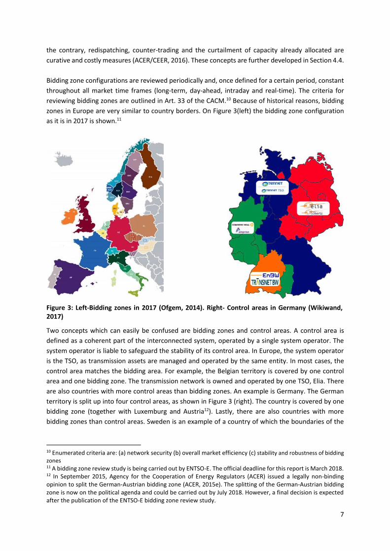
Bidding zone configurations are reviewed periodically and, once defined for a certain period, constant
throughout all market time frames (long-term, day-ahead, intraday and real-time). The criteria for
reviewing bidding zones are outlined in Art. 33 of the CACM.10 Because of historical reasons, bidding
zones in Europe are very similar to country borders. On Figure 3(left) the bidding zone configuration
as it is in 2017 is shown.11
Two concepts which can easily be confused are bidding zones and control areas. A control area is
defined as a coherent part of the interconnected system, operated by a single system operator. The
system operator is liable to safeguard the stability of its control area. In Europe, the system operator
is the TSO, as transmission assets are managed and operated by the same entity. In most cases, the
control area matches the bidding area. For example, the Belgian territory is covered by one control
area and one bidding zone. The transmission network is owned and operated by one TSO, Elia. There
are also countries with more control areas than bidding zones. An example is Germany. The German
territory is split up into four control areas, as shown in Figure 3 (right). The country is covered by one
bidding zone (together with Luxemburg and Austria12). Lastly, there are also countries with more
bidding zones than control areas. Sweden is an example of a country of which the boundaries of the
10 Enumerated criteria are: (a) network security (b) overall market efficiency (c) stability and robustness of bidding zones 11 A bidding zone review study is being carried out by ENTSO-E. The official deadline for this report is March 2018. 12 In September 2015, Agency for the Cooperation of Energy Regulators (ACER) issued a legally non-binding opinion to split the German-Austrian bidding zone (ACER, 2015e). The splitting of the German-Austrian bidding zone is now on the political agenda and could be carried out by July 2018. However, a final decision is expected after the publication of the ENTSO-E bidding zone review study.
Figure 3: Left-Bidding zones in 2017 (Ofgem, 2014). Right- Control areas in Germany (Wikiwand, 2017)
8
control area correspond to the national borders. The Swedish TSO is Svenska Kraftnät. However, the
country is split up into four bidding zones.
Regional: Capacity Calculation Regions (market) and Regional Security Coordinators
(grid & market)
To ensure that cross-zonal transmission capacity calculation is reliable and that optimal capacity is
made available to the market, regional coordination between the TSOs operating the bidding zone
borders is required. This is true as electricity flows in a meshed network are highly interdependent due
to its physical nature.
In order to make coordination happen, Art. 15 of the CACM requires Capacity Calculation Regions
(CCRs) to be determined. A CCR comprises a set of bidding zone borders and is defined as the
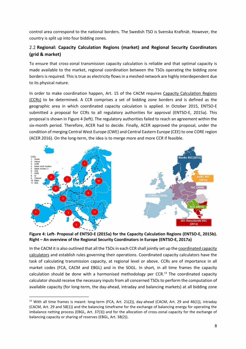
geographic area in which coordinated capacity calculation is applied. In October 2015, ENTSO-E
submitted a proposal for CCRs to all regulatory authorities for approval (ENTSO-E, 2015a). This
proposal is shown in Figure 4 (left). The regulatory authorities failed to reach an agreement within the
six-month period. Therefore, ACER had to decide. Finally, ACER approved the proposal, under the
condition of merging Central West Europe (CWE) and Central Eastern Europe (CEE) to one CORE region
(ACER 2016). On the long-term, the idea is to merge more and more CCR if feasible.
Figure 4: Left- Proposal of ENTSO-E (2015a) for the Capacity Calculation Regions (ENTSO-E, 2015b). Right – An overview of the Regional Security Coordinators in Europe (ENTSO-E, 2017a)
In the CACM it is also outlined that all the TSOs in each CCR shall jointly set up the coordinated capacity
calculators and establish rules governing their operations. Coordinated capacity calculators have the
task of calculating transmission capacity, at regional level or above. CCRs are of importance in all
market codes (FCA, CACM and EBGL) and in the SOGL. In short, in all time frames the capacity
calculation should be done with a harmonised methodology per CCR.13 The coordinated capacity
calculator should receive the necessary inputs from all concerned TSOs to perform the computation of
available capacity (for long-term, the day-ahead, intraday and balancing markets) at all bidding zone
13 With all time frames is meant: long-term (FCA, Art. 21(2)), day-ahead (CACM, Art. 29 and 46(1)), intraday (CACM, Art. 29 and 58(1)) and the balancing timeframe for the exchange of balancing energy for operating the imbalance netting process (EBGL, Art. 37(3)) and for the allocation of cross-zonal capacity for the exchange of balancing capacity or sharing of reserves (EBGL, Art. 38(2)).
9
borders within its CCR. A crucial tool that is created for this purpose is the common grid model, of
which the principles are described both in the FCA and CACM.
Entities strongly tied with CCR are Regional Security Coordinators (RSC) which were registered under
EU law by means of the SOGL. In the SOGL it is stated that each control area shall be covered by at
least one RSC. RSCs are owned or controlled by TSOs and perform tasks related to TSO regional
coordination. The first RSCs were set up as voluntary initiatives (RSCIs) by TSOs since 2008, with
CORESCO (based in Brussels) and TSCNET services (Munich) as pioneers in Continental Europe. In 2015,
one RSC was created in South East Europe (SEE) in Belgrade. In 2016, the Nordic TSOs started discussing
the creation of a Nordic RSC (ENTSO-E, 2017b). An overview of the current RSCs is shown in Figure 4
(right).
RSCs are active in one or more CCR and have five core tasks, mostly related to grid security (for more
details, see e.g. FTI-Compass Lexecon (2016)). RSCs issue recommendations to the TSOs of the capacity
calculation region(s) for which it is appointed. TSOs then should, individually, decide whether to follow
or not the recommendations of the RSC. The TSO remains the final responsible for maintaining
operational security of its control area. One of the tasks of the RSCs is also coordinated capacity
calculation. The link between the coordinated capacity calculators (FCA and CACM) and RSCIs (later
RSCs in SOGL) is described by ENTSO-E (2014, p. 4): “For one Capacity Calculation Region with more
than one established RSCIs, at a given point in time, one RSCI will be responsible for assuming the
function of the Coordinated Capacity Calculator. Other RSCIs having responsibilities within this
Coordinated Capacity Calculation Region can assume this function at any time, as a back-up option.
This scheme ensures consistency between coordinated capacity calculation and coordinated security
assessment.”
Balancing Areas: in between markets and grids
In order to fully grasp the way balancing is conducted in the EU, as described in Chapter 6, some
additional concepts indicating geographical areas of importance for the balancing mechanism need to
be introduced. Also, links between the new balancing concepts and previously introduced bidding
zones and control areas are made in this Section.
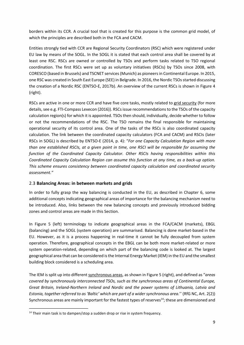
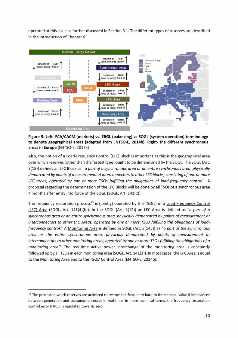
In Figure 5 (left) terminology to indicate geographical areas in the FCA/CACM (markets), EBGL
(balancing) and the SOGL (system operation) are summarised. Balancing is done market-based in the
EU. However, as it is a process happening in real-time it cannot be fully decoupled from system
operation. Therefore, geographical concepts in the EBGL can be both more market-related or more
system operation-related, depending on which part of the balancing code is looked at. The largest
geographical area that can be considered is the Internal Energy Market (IEM) in the EU and the smallest
building block considered is a scheduling area.
The IEM is split up into different synchronous areas, as shown in Figure 5 (right), and defined as “areas
covered by synchronously interconnected TSOs, such as the synchronous areas of Continental Europe,
Great Britain, Ireland-Northern Ireland and Nordic and the power systems of Lithuania, Latvia and
Estonia, together referred to as ‘Baltic’ which are part of a wider synchronous area.’’ (RfG NC, Art. 2(2))
Synchronous areas are mainly important for the fastest types of reserves14; these are dimensioned and
14 Their main task is to dampen/stop a sudden drop or rise in system frequency.
10
operated at this scale as further discussed in Section 6.1. The different types of reserves are described
in the introduction of Chapter 6.
Also, the notion of a Load-Frequency Control (LFC) Block is important as this is the geographical area
over which reserves (other than the fastest type) ought to be dimensioned by the SOGL. The SOGL (Art.
3(18)) defines an LFC Block as ‘’a part of a synchronous area or an entire synchronous area, physically
demarcated by points of measurement at interconnectors to other LFC blocks, consisting of one or more
LFC areas, operated by one or more TSOs fulfilling the obligations of load-frequency control’’. A
proposal regarding the determination of the LFC Blocks will be done by all TSOs of a synchronous area
4 months after entry into force of the SOGL (SOGL, Art. 141(2)).
The frequency restoration process15 is (jointly) operated by the TSO(s) of a Load-Frequency Control
(LFC) Area (SOGL, Art. 141(4)(b)). In the SOGL (Art. 3(12)) an LFC Area is defined as “a part of a
synchronous area or an entire synchronous area, physically demarcated by points of measurement at
interconnectors to other LFC Areas, operated by one or more TSOs fulfilling the obligations of load-
frequency control.” A Monitoring Area is defined in SOGL (Art. 3(145)) as “a part of the synchronous
area or the entire synchronous area, physically demarcated by points of measurement at
interconnectors to other monitoring areas, operated by one or more TSOs fulfilling the obligations of a
monitoring area’’. The real-time active power interchange of the monitoring area is constantly
followed up by all TSOs in each monitoring area (SOGL, Art. 141(3)). In most cases, the LFC Area is equal
to the Monitoring Area and to the TSOs' Control Area (ENTSO-E, 2014b).
15 The process in which reserves are activated to restore the frequency back to the nominal value if imbalances
between generation and consumption occur in real-time. In more technical terms, the frequency restoration
control error (FRCE) is regulated towards zero.
Figure 5: Left- FCA/CACM (markets) vs. EBGL (balancing) vs SOGL (system operation) terminology to denote geographical areas (adapted from ENTSO-E, 2014b). Right- the different synchronous areas in Europe (ENTSO-E, 2017k)

11
Finally, a Scheduling Area is considered the smallest building block for system operation. It is equal to
one or more Control Areas, but can never be bigger than a Bidding Zone. More precisely (SOGL, Art.
110(2)):
• Where a bidding zone covers only one control area (e.g. Belgium), the geographical scope of the scheduling area is equal to the bidding zone.
• Where a control area covers several bidding zones (e.g. Sweden), the geographical scope of the scheduling area is equal to the bidding zone.
• Finally, where a bidding zone covers several control areas (e.g. Germany), TSOs within that bidding zone may jointly decide to operate a common scheduling process. Otherwise, each control area within that bidding zone is considered a separate scheduling area. In this case, the TSOs responsible for the control areas shall agree about which TSO shall operate the scheduling area.
The notion of Scheduling Area is important because important actions related to the balancing
mechanism are done at the level of the scheduling area, i.e.:
• Contractual positions by Balance Responsible Parties (BRPs) are communicated to the TSO of the scheduling area (SOGL, Art. 111(1))
• The measurement of the ‘’system’’ imbalance is done per scheduling area (EBGL, Art. 54(2))
• The Balancing Service Providers (BSPs) participating in the balancing capacity or balancing energy market belong to the same scheduling area (EBGL, Art. 16(8))16.
16 The integration of balancing capacity and energy markets between scheduling areas is the focus of Chapter 7.
12
3. Forward markets
Competitive and liquid forward markets are essential for market participants to hedge their short-term
price risks. Prices in shorter-term electricity markets can fluctuate, e.g. due to high/low renewable
energy infeed. Also, well-functioning short-term markets can deliver sharp scarcity prices. These
scarcity prices are crucial to signal the need for flexibility at particular time and place and to incentivise
new investment (adequacy) in the longer run. However, not all producers want to their business case
to be dependent on hard-to-forecast fluctuating prices and occasional price spikes. Also, large
consumers or retailers might want to stabilise their expenditure. Therefore, there is a demand for
forward markets with long-term contracts for electricity supply. Newbery (2016) states ”a lack of
forward markets and long-term contracts might not be so critical if the future were reasonably
predictable and stable, but that this is far from the case at present.” Also Genoese et al. (2016) and
Neuhoff et al. (2016) argue that the provision of long-term price signals will become (even) more
important in the future, one important argument is that long-term contracts can reduce the cost of
capital of renewables and flexible generation, characterised by high upfront investment costs.
The integration of forward energy markets is crucial to allow a more efficient functioning and higher
degrees of necessary liquidity. Therefore, long-term cross-zonal transmission rights are auctioned. By
acquiring these rights, agents can also trade cross-border in forward markets. Without these rights,
the risk related to price differentials between different bidding zones can significantly reduce the
appeal of such cross-border trades. Also, cross-zonal transmission rights are of importance to be able
to hedge risk across different timeframes within a certain bidding zone. This would be the case when
long-term electricity contracts (the commodity) with few different durations are offered within a
bidding zone, while in another bidding zone (a so-called hub) contracts with many different durations
are offered.
First, forward energy markets are introduced in this chapter. After the integration of forward markets
is discussed, the implications of the FCA guideline are highlighted.
Forward energy markets
Long-term electricity contracts can be traded on unstandardized forward and standardised future
markets. The design of the (national) forward electricity markets is not covered by the network codes.
Instead, the way in which long-term cross-zonal transmission rights are allocated is the focus of the
FCA. Long-term cross-zonal transmission rights are needed to allow the integration of these forward
markets. Integration can help these markets function more efficiently.
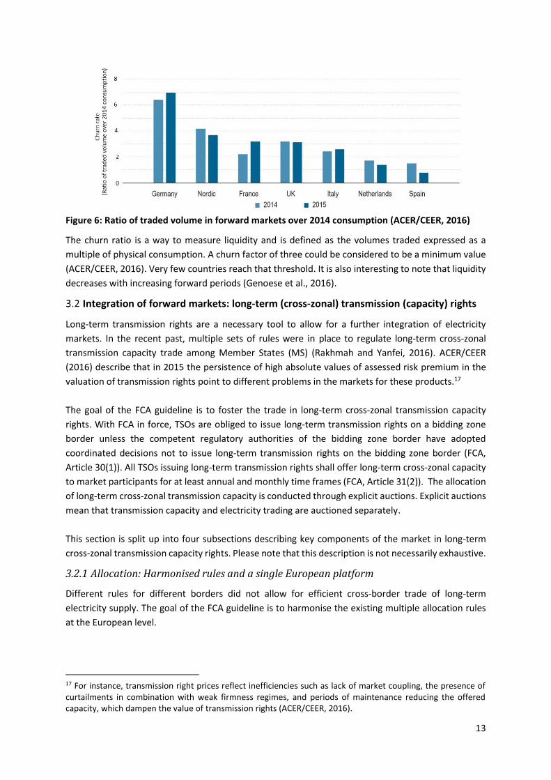
The analysis in ACER/CEER (2016) shows that, in general, the liquidity of forward markets in Europe
remained low in 2015, except for Germany, the Nordics, France and GB. In Figure 6, the churn ratio for
the most relevant European countries is shown.
13
Figure 6: Ratio of traded volume in forward markets over 2014 consumption (ACER/CEER, 2016)
The churn ratio is a way to measure liquidity and is defined as the volumes traded expressed as a
multiple of physical consumption. A churn factor of three could be considered to be a minimum value
(ACER/CEER, 2016). Very few countries reach that threshold. It is also interesting to note that liquidity
decreases with increasing forward periods (Genoese et al., 2016).
Integration of forward markets: long-term (cross-zonal) transmission (capacity) rights
Long-term transmission rights are a necessary tool to allow for a further integration of electricity
markets. In the recent past, multiple sets of rules were in place to regulate long-term cross-zonal
transmission capacity trade among Member States (MS) (Rakhmah and Yanfei, 2016). ACER/CEER
(2016) describe that in 2015 the persistence of high absolute values of assessed risk premium in the
valuation of transmission rights point to different problems in the markets for these products.17
The goal of the FCA guideline is to foster the trade in long-term cross-zonal transmission capacity
rights. With FCA in force, TSOs are obliged to issue long-term transmission rights on a bidding zone
border unless the competent regulatory authorities of the bidding zone border have adopted
coordinated decisions not to issue long-term transmission rights on the bidding zone border (FCA,
Article 30(1)). All TSOs issuing long-term transmission rights shall offer long-term cross-zonal capacity
to market participants for at least annual and monthly time frames (FCA, Article 31(2)). The allocation
of long-term cross-zonal transmission capacity is conducted through explicit auctions. Explicit auctions
mean that transmission capacity and electricity trading are auctioned separately.
This section is split up into four subsections describing key components of the market in long-term
cross-zonal transmission capacity rights. Please note that this description is not necessarily exhaustive.
3.2.1 Allocation: Harmonised rules and a single European platform
Different rules for different borders did not allow for efficient cross-border trade of long-term
electricity supply. The goal of the FCA guideline is to harmonise the existing multiple allocation rules
at the European level.
17 For instance, transmission right prices reflect inefficiencies such as lack of market coupling, the presence of curtailments in combination with weak firmness regimes, and periods of maintenance reducing the offered capacity, which dampen the value of transmission rights (ACER/CEER, 2016).
14
A first step in that direction is to introduce harmonised allocation rules (HAR) for long-term
transmission rights. According to the FCA, all TSOs had to submit a proposal for these rules 6 months
after the entry into force of the Regulation (FCA, Art. 51(1)) covering several aspects in the forward
capacity allocation (FCA, Art. 52), inter alia returns and transfers of long-term transmission rights. In
addition to these harmonised allocation rules, specific regional requirement or requirements for
individual borders where long-term transmission rights are allocated can be proposed (FCA, Art. 51(1)).
Given the importance of this task, TSOs have proposed harmonised allocation rules already before the
entry into force of the FCA as part of the early implementation of the FCA. In the framework of the
official implementation of the FCA, all TSOs submitted the proposal of the harmonised allocation rules
and the specific border/regional requirements in April 2017 (ENTSO-E, 2017c).
Moreover, a key instrument towards the integration of cross-zonal long-term markets is the setup of
a single European platform for the allocation of long-term cross-zonal transmission rights. Some steps
have already been taken in that direction. On 24 June 2015, the two regional allocation offices for
cross-zonal electricity transmission capacities in place at that time, approved the merger agreement
to create the Joint Allocation Office (JAO). The JAO is a joint service company of twenty TSOs from
seventeen countries. It performs mainly the yearly, monthly and daily auctions of transmission rights
on 27 borders in Europe. In their proposal for the Single Allocation Platform submitted in April 2017,
all TSOs proposed that JAO be named as the Single Allocation Platform (ENTSO-E, 2017d).
A practical example of the importance of a single European platform and harmonised allocation rules
is the timing and length of different cross-zonal transmission rights. If long-term transmission rights
are not allocated simultaneously, agents who need to ‘cross’ several borders cannot efficiently hedge
their cross-zonal short-term price risk.
3.2.2 Calculation of future cross-zonal transmission capacity
As stated in the FCA guideline: “Long-term capacity calculation for the year- and month-ahead market
time frames should be coordinated by the TSOs at least at regional level to ensure that capacity
calculation is reliable and that optimal capacity is made available to the market.”
What ‘’coordination on regional level” exactly aims at are that calculations done at the level of the
Capacity Calculation Regions (CCR). Capacity Calculation Regions (CCR) are described in Section 2.2.
For this purpose, TSOs should establish a common grid model gathering all the necessary data for the
long-term capacity calculation and taking into account the uncertainties inherent to the long-term time
frames.
Long-term capacity calculation can be done applying two approaches: the flow-based approach and
the coordinated net transmission capacity (NTC) approach. These calculation methods are explained
in more detail in 5.1.2. The FCA leaves it open which approach should be applied. However, it is
mentioned that the flow-based approach might be justified where cross-zonal capacities between
bidding zones are highly interdependent.
3.2.3 Products and pricing
Two products for long-term cross-zonal transmission capacity rights are described in the FCA;
definitions are taken from Batlle et al. (2014):
15
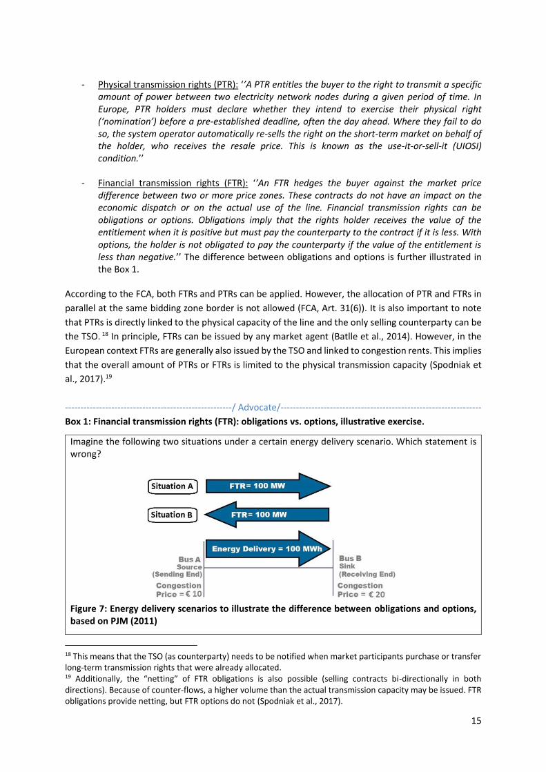
- Physical transmission rights (PTR): ‘’A PTR entitles the buyer to the right to transmit a specific amount of power between two electricity network nodes during a given period of time. In Europe, PTR holders must declare whether they intend to exercise their physical right (‘nomination’) before a pre-established deadline, often the day ahead. Where they fail to do so, the system operator automatically re-sells the right on the short-term market on behalf of the holder, who receives the resale price. This is known as the use-it-or-sell-it (UIOSI) condition.’’
- Financial transmission rights (FTR): ‘’An FTR hedges the buyer against the market price difference between two or more price zones. These contracts do not have an impact on the economic dispatch or on the actual use of the line. Financial transmission rights can be obligations or options. Obligations imply that the rights holder receives the value of the entitlement when it is positive but must pay the counterparty to the contract if it is less. With options, the holder is not obligated to pay the counterparty if the value of the entitlement is less than negative.’’ The difference between obligations and options is further illustrated in the Box 1.
According to the FCA, both FTRs and PTRs can be applied. However, the allocation of PTR and FTRs in
parallel at the same bidding zone border is not allowed (FCA, Art. 31(6)). It is also important to note
that PTRs is directly linked to the physical capacity of the line and the only selling counterparty can be
the TSO. 18 In principle, FTRs can be issued by any market agent (Batlle et al., 2014). However, in the
European context FTRs are generally also issued by the TSO and linked to congestion rents. This implies
that the overall amount of PTRs or FTRs is limited to the physical transmission capacity (Spodniak et
al., 2017).19
------------------------------------------------------/ Advocate/-----------------------------------------------------------------
Box 1: Financial transmission rights (FTR): obligations vs. options, illustrative exercise.
Imagine the following two situations under a certain energy delivery scenario. Which statement is wrong?
Figure 7: Energy delivery scenarios to illustrate the difference between obligations and options, based on PJM (2011)
18 This means that the TSO (as counterparty) needs to be notified when market participants purchase or transfer long-term transmission rights that were already allocated. 19 Additionally, the “netting” of FTR obligations is also possible (selling contracts bi-directionally in both directions). Because of counter-flows, a higher volume than the actual transmission capacity may be issued. FTR obligations provide netting, but FTR options do not (Spodniak et al., 2017).
16
a.) If I hold a FTR-option in situation A, I gain €1000 b.) If I hold a FTR-obligation in situation A, I gain €1000 c.) If I hold a FTR-option in situation B, I lose €1000 d.) If I hold a FTR-obligation in situation B, I lose €1000 Correct answer: c Justification: In situation A, the outcome for an option and an obligation are the same. The holder of the both FTR gain (20 €/MWh-10 €/MWh)*100 MWh= €1000. In situation B only the holder of a FTR-obligation has to pay (20 €/MWh-10 €/MWh)*-100 MWh= -€1000. A holder of an option will not exercise the option in this case and would not lose any money (except the price paid beforehand for acquiring the option). In other words, in situation A both FTR-obligations and options are a benefit. In situation B, a FTR-obligation is a liability, while a FTR-option is neither a liability or benefit.
Batlle et al. (2014) describe in detail the pro and cons of PTRs and FTRs. They split their analysis into
two parts. Firstly, an ideal market operation and structure is assumed.20 In that situation, PTRs and
FTRs are equivalent. Secondly, an analysis is done under the conditions prevailing in real electricity
markets, paying particular attention to situations where market power can be exercised. In that case,
there are material differences between both products. The authors conclude that if there is sufficient
inter-market coordination and liquidity, FTRs should be the preferred product. However, until these
conditions are not attained, PTRs are the most suitable transitory solution. The advantages of FTRs
over PTRs found are greater transparency, simplification of regulatory supervision and provision of a
more valuable hedge for minority market share agents. With PTRs market agents with physical
generation assets are clearly in a better position to engage in trading. This is not the case for FTRs, and
therefore FTRs would broaden the demand base, enhance competition and increase market liquidity.
PTRs versus FTRs has been a strongly debated topic in the academic literature for a long period. Overall,
many arguments are found in favour of FTRs, examples of relevant work are Benjamin (2010), Chao
and Peck (1996), Hogan (1992) and Joskow and Tirole (2000).
Box 2: The Nordic approach to long-term transmission rights (based on Spodniak et al. (2017))
Since 2000, the Nordic electricity market has its own standard product in use for hedging bidding area price differences, called the “electricity area price differential” (EPAD). EPAD contracts are used to build a hedge for a bidding area price in relation to the Nordic system price (a sort of benchmark price, there is no similar system price in the rest of Europe), while an FTR contract hedges the price difference directly between two adjacent bidding areas. To hedge the price difference between two adjacent bidding areas with EPADs as an FTR would do, a combination of two EPAD contracts (a so-called EPAD Combos) needs to be acquired by a market player. Two EPAD Combos are required to cover the hedge “both ways” for each interconnector between two bidding zones. Spodniak et al. (2017) note “this replication implies that it is theoretically and even practically possible to continue with the EPAD-based system by using EPAD Combos in the Nordic countries, even if FTR contracts would prevail elsewhere in the EU.” Additionally, the authors do an empirical analysis and show that in practice the pricing of bi-directional EPAD contracts is more complex and may not always be very efficient.
20 According to Batlle et al. (2014), an ideal market would imply: the absence of technical conditioning (physical flows equal commercial transactions), no regulatory design inefficiencies, unlimited liquidity, no transactions costs, no market power and fully rational market players.

17
A significant difference between FTRs and EPADs is that EPADs are purely financial contracts traded on a securities exchange, without a direct link to the transmission capacity of the interconnectors. As such, there is also no volume cap in terms of offered transmission rights.
--------------------------------------------------------------------------------------------------------------------------------------
Also in the work of Batlle et al. (2014), FTR-obligations versus FTR-options are discussed. A major
difference between both is that obligations are allocated simultaneously in both directions (one
product, one auction), while an option only covers the price risk in one direction (two products, two
auctions). Although possible higher implementation costs and decreased liquidity can be expected
with options, it is argued that these are favoured by market players as in most cases market players
are interested in hedging the price risk in solely one direction.
Regarding pricing, the FCA states in Article 28 that marginal pricing should be applied for each bidding
zone border, direction and market time unit. Marginal pricing implies that all successful bidders pay
the price of the marginally accepted bid (in this case the lowest accepted bid). The price will equal zero
if the demand for transmission rights is lower than the offered quantity.
3.2.4 Firmness
Trust in firmness, defined in the CACM as ‘’a guarantee that cross-zonal capacity rights will remain
unchanged and that a compensation is paid if they are nevertheless changed’’, is a necessary condition
for the successful integration of electricity markets. The potential interruption of exports during
emergency or scarcity conditions can be a major barrier to the development of (long-term) cross-zonal
trade (Mastropietro et al., 2015).
In the FCA, two causes for curtailment of long-term transmission rights are distinguished. Firstly, the
curtailment of transmission rights in the event of force majeure21. In that case, the holder of long-term
transmission rights will receive a compensation equal to the amount initially paid for long-term
transmission right (FCA, Art. 56(3)). The national regulatory authority of the TSO invoking the force
majeure event shall assess whether an event qualifies as force majeure (FCA, Art. 56(5). Secondly, long-
term transmission rights can also be curtailed prior to the day-ahead firmness deadline to ensure that
operation remains within operational security limits. The concerned TSOs on the bidding zone border
where long-term transmission rights have been curtailed shall compensate the holder of these rights
with the market spread22 (FCA, Art. 53(2)). Further, the concerned TSOs on a bidding zone border may
propose a cap23 on the total compensation to be paid to all holders of curtailed long-term transmission
rights (FCA, Art. 54(1)).
------------------------------------------------------/ Advocate/-----------------------------------------------------------------
21 A force majeure event is defined in the CACM as any unforeseeable or unusual event or situation beyond the reasonable control of a TSO, and not due to a fault of the TSO, which cannot be avoided or overcome with reasonable foresight and diligence, which cannot be solved by measures which are from a technical, financial or economic point of view reasonably possible for the TSO, which has actually happened and is objectively verifiable, and which makes it impossible for the TSO to fulfil, temporarily or permanently, its obligations in accordance with this Regulation (CACM). 22 With the market spread is meant the difference between the hourly day-ahead prices of the two concerned bidding zones for the respective market time unit in a specific direction. 23 The cap holds for the accumulated compensations over the relevant calendar year and cannot be lower than the total congestion income collected during that same period (FCA, Art. 54(1,2)).

18
Mastropietro et al. (2015) argue that congestion is not the only source of price-differentials between
bidding zones. They state that price-differentials may also be originated by a direct regulatory
intervention to prioritise national over regional interests. This would be the case if a TSO (prompt by a
regulator) blocks exports through interconnectors when its system is under scarcity conditions. By
doing so, a price-differential is artificially created wherefore no hedge exists, and the execution of
cross-border contracts is impeded. Mastropietro et al. (2015) add that, whenever the physical delivery
is not possible because of an intervention from the TSO, the latter should pay not only the financial
settlement related to the price differentials but additionally possibly a compensation. This
compensation equals the penalty for non-compliance24 a generator located in one bidding zone should
pay to a demand located in another bidding zone when these two parties have signed a contract for
the physical delivery of electricity, and the demand is not served. The TSO (representing the regulator
and, eventually, the government) should also be required to deposit warranties for the coverage of
such payments.
It is of great importance that the risks are properly allocated, if not the TSO might become more risk-
averse and offer less long-term capacity than would be efficient or market players might be
disincentivised to engage in long-term cross-zonal trade.
--------------------------------------------------------------------------------------------------------------------------------------
24 The compensation is related to the difference between the utility value that the demand attributes to its supply and the price cap active in the market (Mastropietro et al., 2015).

19
4. Establishing national day-ahead and intraday markets
The CACM is the key regulation outlining the design and integration of the day-ahead (DA) and intraday
market (IDM). In this chapter, we focus on the establishment of the national DA and IDMs25. Their
integration is discussed in Chapter 5. The ‘Target Model’ pursued by the European Commission (Third
Energy Package, Directive 2009/72/EC) is centred on day-ahead auctions operated by power
exchanges that implicitly allocate transmission capacity between bidding zones (Neuhoff et al., 2016c).
Prices obtained in the DAM auction serve as a reference for forward markets (Meeus, 2011). In the last
years, a strong increase trading closer in intraday markets was observed, as is illustrated in Figure 8
(below). On that same figure, the trading volumes in the DAM as a share of the hourly consumption
for France and Germany for a period from 2012 to 2015 are shown. It can be seen that large differences
in proportional volumes exist between both countries. It can be argued that the centre of gravity of
electricity trading is slowly shifting to markets closer to real-time.
Figure 8: The hourly DA and ID market trading volume as share of the hourly consumption for France and Germany (Brijs et al., 2017)
Short-term electricity market design needs to evolve with its context. Originally, these markets were
designed for large, rather slow ramping, and mostly fossil fuel based generators and inflexible demand.
Today, the same conditions do not hold anymore with the penetration of variable renewable energy
sources (vRES) at all voltage levels and more options for consumers to steer their demand. It is highly
25 National DA and IDMs can have for instance additional products (e.g. with a finer time granularity) next to the products traded in the single European (coupled) DA and IDM. These products are traded after the cross-border DA gate closure time and are only national, bilateral or regional but not EU wide.
20
debated how to adjust market design to this new context (for e.g. AGORA, 2016; Brijs et al., 2017;
Henriot and Glachant, 2013; Neuhoff et al., 2016, 2015b). In general, it is agreed upon that flexibility
is required for the system. Short-term electricity market design should encourage investment in the
right technologies (capacity) and incentivize them to offer their full flexibility (capability). A
combination of complementary actions is needed to achieve this goal. Integration of electricity
markets at all market time frames is key. Also, day-ahead market design needs to be adapted, for
example by introducing better-adapted bidding products. Further, the functioning of markets closer to
real-time needs to be enhanced, both intraday and balancing markets (treated in Chapter 6).
In this chapter, firstly, a key institution, namely the Nominated Electricity Market Operator (NEMO)
and its functions are described. The DAM and IDM are both managed by power exchanges, which are
now labelled as NEMOs, a concept introduced by the CACM. After, the main characteristics of the day-
ahead market are discussed. Lastly, an overview of discussed elements of intraday market design is
given.
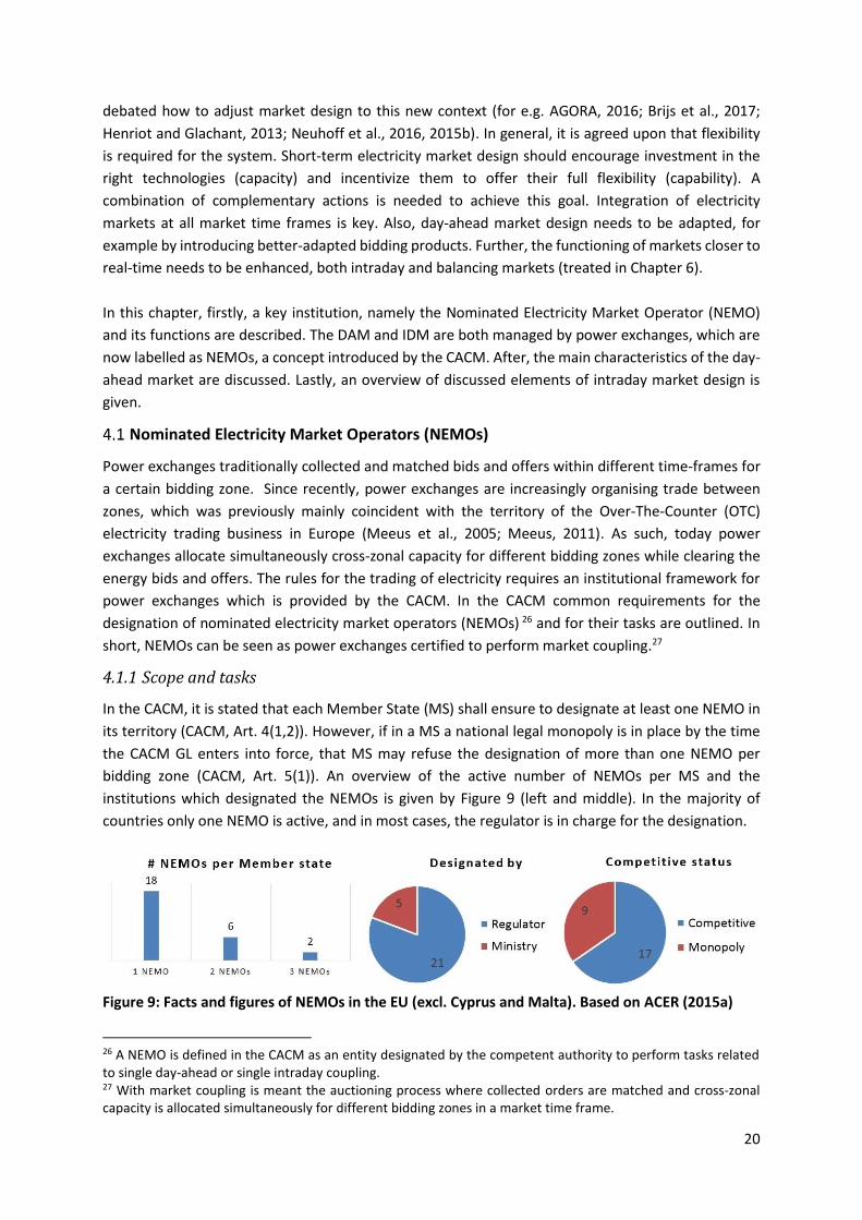
Nominated Electricity Market Operators (NEMOs)
Power exchanges traditionally collected and matched bids and offers within different time-frames for
a certain bidding zone. Since recently, power exchanges are increasingly organising trade between
zones, which was previously mainly coincident with the territory of the Over-The-Counter (OTC)
electricity trading business in Europe (Meeus et al., 2005; Meeus, 2011). As such, today power
exchanges allocate simultaneously cross-zonal capacity for different bidding zones while clearing the
energy bids and offers. The rules for the trading of electricity requires an institutional framework for
power exchanges which is provided by the CACM. In the CACM common requirements for the
designation of nominated electricity market operators (NEMOs) 26 and for their tasks are outlined. In
short, NEMOs can be seen as power exchanges certified to perform market coupling.27
4.1.1 Scope and tasks
In the CACM, it is stated that each Member State (MS) shall ensure to designate at least one NEMO in
its territory (CACM, Art. 4(1,2)). However, if in a MS a national legal monopoly is in place by the time
the CACM GL enters into force, that MS may refuse the designation of more than one NEMO per
bidding zone (CACM, Art. 5(1)). An overview of the active number of NEMOs per MS and the
institutions which designated the NEMOs is given by Figure 9 (left and middle). In the majority of
countries only one NEMO is active, and in most cases, the regulator is in charge for the designation.
Figure 9: Facts and figures of NEMOs in the EU (excl. Cyprus and Malta). Based on ACER (2015a)
26 A NEMO is defined in the CACM as an entity designated by the competent authority to perform tasks related to single day-ahead or single intraday coupling. 27 With market coupling is meant the auctioning process where collected orders are matched and cross-zonal capacity is allocated simultaneously for different bidding zones in a market time frame.
21
A NEMO can be designed for trading services in the day-ahead market, the intraday market or both.
Today, all designated NEMOs offer services in both markets (ACER, 2015a). NEMO(s) designated in a
MS have the right to offer trading services with delivery in another MS without the need for
designation as a NEMO in that Member State, however with exemptions. These exemptions are
summed up in Article 4(6) of the CACM.
In CACM, Article 7(1) the tasks of the NEMOs are outlined, the article says” Their [NEMOs] tasks shall
include receiving orders from market participants, having overall responsibility for matching and
allocating orders in accordance with the single day-ahead and intraday coupling results, publishing
prices and settling and clearing the contracts resulting from the trades according to relevant participant
agreements and regulations.’’ Also, all NEMOs shall, in cooperation with the relevant TSOs, develop a
proposal on harmonised maximum and minimum clearing prices to be applied in all bidding zones. A
proposal shall be made for the DAM and another for the IDM. NEMOs shall carry out market coupling
operator (MCO) functions jointly with other NEMOs, for this purpose also a close collaboration with
coordinated capacity calculators28 is required.
4.1.2 Cost-of-service regulated versus merchant
Meeus (2011) states that two types of power exchanges have to be distinguished in Europe: cost-of-
service regulated (monopoly) and merchant (competitive) power exchanges. Cost-of-service regulated
are not-for-profit or regulated-profit institutions which receive an income through regulated fees. They
can be established by a public initiative (e.g. OMEL in Spain) or by a TSO initiative (e.g. HUPX in
Hungary). Typically, they also perform several tasks that go beyond trading services. On the other hand,
merchant power exchanges are for-profit market institutions whose core business is to provide trading
services. Their income depends on various user fees and is linked to the volume of trades executed by
the power exchange for its users. Examples are EPEX Spot (covering Germany, France, UK, the
Netherlands, Belgium, Austria, Switzerland and Luxembourg) and Nord Pool AS (one of the NEMO(s)
or single NEMO in 15 European countries). Historically, merchants were set up by market parties,
financial market institutions, TSOs or a combination of private actors. On Figure 9 (right), the
competitive status of a power exchange in the Member States is shown. In most countries, power
exchanges are a competitive activity, however, in nine countries (e.g. Italy and Spain) they have a
monopoly status.
The CACM leaves it open whether NEMOs should be a monopoly or competitive activity. However, in
the spirit of the code, a preference for NEMOs as a competitive activity can be detected. Namely, it is
stated “a national legal monopoly is deemed to exist where national law expressly provides that no
more than one entity within a Member State or Member State bidding zone can carry out day-ahead
and intraday trading services” (CAMC GL, Art. 5(2)). However, “if the Commission deems that there is
no justification for the continuation of national legal monopolies or for the continued refusal of a MS
to allow cross-border trading by a NEMO designated in another MS, the Commission may consider
appropriate legislative or other appropriate measures to further increase competition and trade
between and within MSs” (CACM, Art. 5(3)).
------------------------------------------------------/ Advocate/-----------------------------------------------------------------
28 In short, a coordinated capacity calculator (CCC) is set up jointly by a subset of TSOs (CACM, Art. 2(11)), and calculates the available cross-zonal transmission capacity per capacity calculation region (CCR).
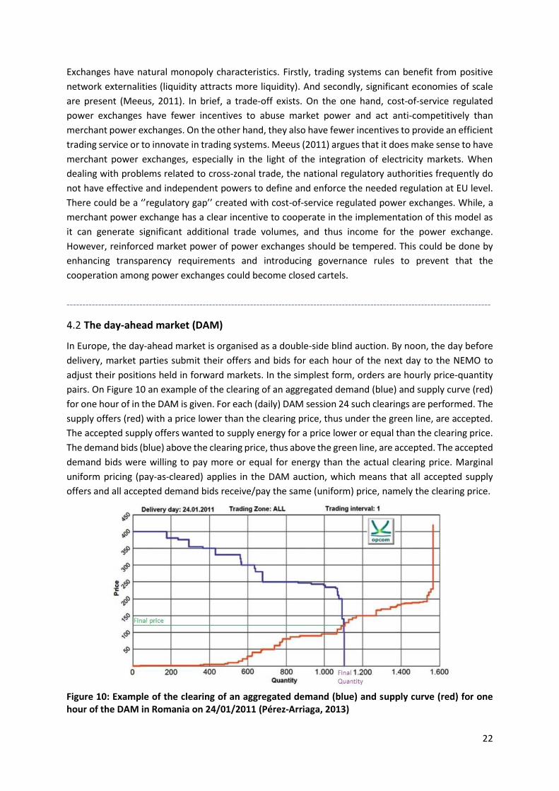
22
Exchanges have natural monopoly characteristics. Firstly, trading systems can benefit from positive
network externalities (liquidity attracts more liquidity). And secondly, significant economies of scale
are present (Meeus, 2011). In brief, a trade-off exists. On the one hand, cost-of-service regulated
power exchanges have fewer incentives to abuse market power and act anti-competitively than
merchant power exchanges. On the other hand, they also have fewer incentives to provide an efficient
trading service or to innovate in trading systems. Meeus (2011) argues that it does make sense to have
merchant power exchanges, especially in the light of the integration of electricity markets. When
dealing with problems related to cross-zonal trade, the national regulatory authorities frequently do
not have effective and independent powers to define and enforce the needed regulation at EU level.
There could be a ‘’regulatory gap’’ created with cost-of-service regulated power exchanges. While, a
merchant power exchange has a clear incentive to cooperate in the implementation of this model as
it can generate significant additional trade volumes, and thus income for the power exchange.
However, reinforced market power of power exchanges should be tempered. This could be done by
enhancing transparency requirements and introducing governance rules to prevent that the
cooperation among power exchanges could become closed cartels.
--------------------------------------------------------------------------------------------------------------------------------------
The day-ahead market (DAM)
In Europe, the day-ahead market is organised as a double-side blind auction. By noon, the day before
delivery, market parties submit their offers and bids for each hour of the next day to the NEMO to
adjust their positions held in forward markets. In the simplest form, orders are hourly price-quantity
pairs. On Figure 10 an example of the clearing of an aggregated demand (blue) and supply curve (red)
for one hour of in the DAM is given. For each (daily) DAM session 24 such clearings are performed. The
supply offers (red) with a price lower than the clearing price, thus under the green line, are accepted.
The accepted supply offers wanted to supply energy for a price lower or equal than the clearing price.
The demand bids (blue) above the clearing price, thus above the green line, are accepted. The accepted
demand bids were willing to pay more or equal for energy than the actual clearing price. Marginal
uniform pricing (pay-as-cleared) applies in the DAM auction, which means that all accepted supply
offers and all accepted demand bids receive/pay the same (uniform) price, namely the clearing price.
Figure 10: Example of the clearing of an aggregated demand (blue) and supply curve (red) for one hour of the DAM in Romania on 24/01/2011 (Pérez-Arriaga, 2013)
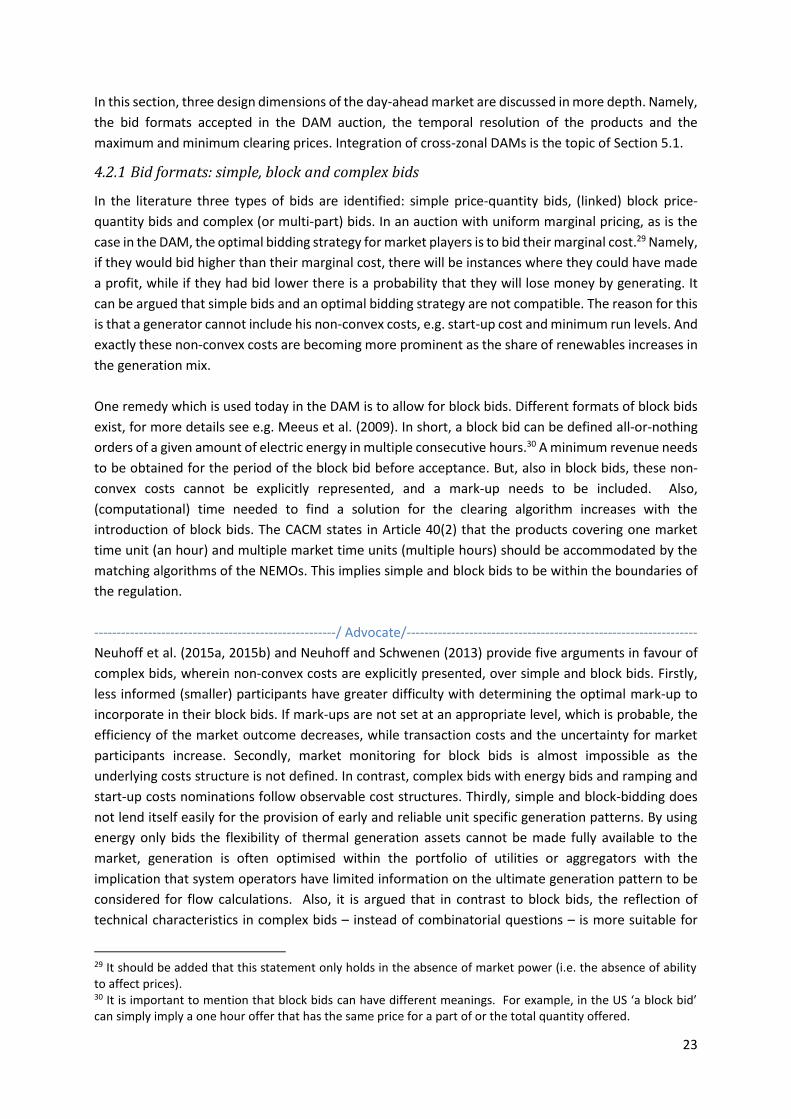
23
In this section, three design dimensions of the day-ahead market are discussed in more depth. Namely,
the bid formats accepted in the DAM auction, the temporal resolution of the products and the
maximum and minimum clearing prices. Integration of cross-zonal DAMs is the topic of Section 5.1.
4.2.1 Bid formats: simple, block and complex bids
In the literature three types of bids are identified: simple price-quantity bids, (linked) block price-
quantity bids and complex (or multi-part) bids. In an auction with uniform marginal pricing, as is the
case in the DAM, the optimal bidding strategy for market players is to bid their marginal cost.29 Namely,
if they would bid higher than their marginal cost, there will be instances where they could have made
a profit, while if they had bid lower there is a probability that they will lose money by generating. It
can be argued that simple bids and an optimal bidding strategy are not compatible. The reason for this
is that a generator cannot include his non-convex costs, e.g. start-up cost and minimum run levels. And
exactly these non-convex costs are becoming more prominent as the share of renewables increases in
the generation mix.
One remedy which is used today in the DAM is to allow for block bids. Different formats of block bids
exist, for more details see e.g. Meeus et al. (2009). In short, a block bid can be defined all-or-nothing
orders of a given amount of electric energy in multiple consecutive hours.30 A minimum revenue needs
to be obtained for the period of the block bid before acceptance. But, also in block bids, these non-
convex costs cannot be explicitly represented, and a mark-up needs to be included. Also,
(computational) time needed to find a solution for the clearing algorithm increases with the
introduction of block bids. The CACM states in Article 40(2) that the products covering one market
time unit (an hour) and multiple market time units (multiple hours) should be accommodated by the
matching algorithms of the NEMOs. This implies simple and block bids to be within the boundaries of
the regulation.
------------------------------------------------------/ Advocate/-----------------------------------------------------------------
Neuhoff et al. (2015a, 2015b) and Neuhoff and Schwenen (2013) provide five arguments in favour of
complex bids, wherein non-convex costs are explicitly presented, over simple and block bids. Firstly,
less informed (smaller) participants have greater difficulty with determining the optimal mark-up to
incorporate in their block bids. If mark-ups are not set at an appropriate level, which is probable, the
efficiency of the market outcome decreases, while transaction costs and the uncertainty for market
participants increase. Secondly, market monitoring for block bids is almost impossible as the
underlying costs structure is not defined. In contrast, complex bids with energy bids and ramping and
start-up costs nominations follow observable cost structures. Thirdly, simple and block-bidding does
not lend itself easily for the provision of early and reliable unit specific generation patterns. By using
energy only bids the flexibility of thermal generation assets cannot be made fully available to the
market, generation is often optimised within the portfolio of utilities or aggregators with the
implication that system operators have limited information on the ultimate generation pattern to be
considered for flow calculations. Also, it is argued that in contrast to block bids, the reflection of
technical characteristics in complex bids – instead of combinatorial questions – is more suitable for
29 It should be added that this statement only holds in the absence of market power (i.e. the absence of ability to affect prices). 30 It is important to mention that block bids can have different meanings. For example, in the US ‘a block bid’ can simply imply a one hour offer that has the same price for a part of or the total quantity offered.

24
computation of market clearing. Lastly, with block bids liquidity in standardised auctions might be
undermined as bids only are valid conditional on being accepted for longer time durations. Today,
complex bids are present mostly in the US electricity markets, but also in some European markets, e.g.
Spain and Poland (Brijs et al., 2017; Neuhoff et al., 2016c).
A commonly used argument against complex bids made by generators is that they would need to
reveal commercially sensitive information in their bids. Neuhoff et al. (2015b) state that it is expected
that the level of information sharing will not be extended beyond the level of sharing that is already
necessary with TSOs. Meeus and Belmans (2007) state that with block-bids the pricing approach in
dealing with non-convexities is simpler than with complex bids. Arguably, it can be harder to couple
markets allowing for complex bids because they can apply a different implementation of non-linear
pricing internally.31 The reason is that it is politically difficult to harmonise the treatment of non-
convexities and especially if the treatment is already fine-tuned, which is less the case with easier-to-
harmonise block bids. The CACM states that NEMOs shall submit a joint proposal concerning products
that can be taken into account in the single day-ahead market coupling (CACM, Art. 40(1)). It is added
that the orders resulting from these products should be expressed in euros and make reference to the
market time.
--------------------------------------------------------------------------------------------------------------------------------------
4.2.2 Temporal granularity
Today, in the European DAM the market time unit of traded products is one hour. This granularity in
the DAM is not directly seen as problematic in the academic literature, under the condition that
products with finer resolution are offered in intraday markets and/or locally. However, it is
straightforward that the finer the granularity, the more volatile the prices will be. These prices can
better reflect and reward the value of flexibility in the system. Units can take advantage of price
volatility when they can ramp up or ramp down faster. Flexible resources need clear signals to
encourage investment and to deliver energy when they are needed and, shorter time-unit can deliver
these incentives.
------------------------------------------------------/ Advocate/-----------------------------------------------------------------
Also, some issues might occur as the settlement period over which market participants are financially
responsible for having a balanced portfolio is 15 minutes or half-hour.32 Therefore, shorter market
periods would allow for a better alignment of trading in the DAM and imbalances in real-time (Brijs et
al., 2017). If demand and supply schedules are scheduled on a shorter time interval, reserve
requirements might be reduced (Neuhoff et al., 2015a). Shorter time-units also help in shifting the risks
from TSOs to market parties responsible for balancing their demand and supply33 (Frunt, 2011). Less
31 Without going into too much technical details, when allowing for block bids and/or complex bids, it is not always feasible to find a clearing price wherefore all accepted offers are in-the-money (not making losses), or wherefore all rejected offers are out-of-the-money (making money). Broadly speaking, in the US, with complex bids, some accepted offers are making losses when considering solely the clearing price. This problem is solved with uplift payments. In Europe, with block bids, some rejected block offers could be making money considering the clearing price, these are so called ‘’paradoxically rejected blocks’’ (Meeus et al., 2009). See also, section 2.2.2. in Papavasiliou and Smeers (2017). 32 For more details, please consults Chapter 6 in which the balancing mechanism is presented. 33 So called “Balance Responsible Party (BRP)’’, explained in the introduction of Chapter 6.

25
intervention from the TSO will normally be required, and thus fewer costs will need to be socialised
(Henriot and Glachant, 2013). Lastly and related to the previous remark, by having more granular
products the deterministic imbalances, as mentioned by Hirth and Ziegenhagen (2015), will be more
limited and balancing costs, in the case passive balancing is not allowed, will be decreased.
Counterarguments are that non-convexities are even harder to include in simple bids with finer
temporal granularity and that the computational time might increase strongly to clear the market as
more combinations are possible (Henriot and Glachant, 2013). Neuhoff et al. (2016) explain that the
finer the granularity of the bids, the higher the need for complex bids will be.
--------------------------------------------------------------------------------------------------------------------------------------
4.2.3 Maximum and minimum clearing prices
A general remark made in the literature is that price caps and floors should be removed as they distort
the price signal and will cause peak units or more flexible resources not to recover their capital costs,
contributing to the ‘missing-money’ problem. There is no theoretical rationale for a limit to price floors
(Henriot and Glachant, 2013) and with more participation of the demand side, increasing storage
possibilities and a weaker presence of market power there are fewer reasons to hold on to price caps
as well. No price caps will give market participants a high degree of planning security. Additionally,
Hogan (2013) argues that higher price caps are a necessary, but not sufficient condition, to be
consistent with a reasonable market for addressing scarcity conditions. However, in terms of scarcity,
it would be difficult or impossible to distinguish real scarcity in supply from the exercise of market
power.
In the CACM, it is outlined that NEMOs, in cooperation with TSOS, shall develop a proposal on
harmonised maximum and minimum prices to be applied in all bidding zones which participate in single
day-ahead coupling (CAMC, Art. 41).
The intraday market (IDM)
Higher shares of wind and solar generation result in increasing volumes of intraday trading (see also
Figure 8 (below) on page 19). Closer to real-time, wind- and solar (but also demand) forecasts are more
accurate and in intraday markets production schedules can be adjusted accordingly. While the day-
ahead market design is quite harmonised in the EU, the same cannot be said about intraday market
design. In some countries, e.g. Belgium, France and the Netherlands, shortly after the DAM auction,
continuous trading with hourly products is possible (Brijs et al., 2017). In other countries, e.g. Spain,
multiple intraday auctions with 15-minute products are held (Hagemann and Weber, 2015). In
Germany, a combination of continuous trade and auctions is in place (Neuhoff et al., 2016b). As an
illustration, in Figure 11 the EPEX trading process in Germany is shown in more detail.
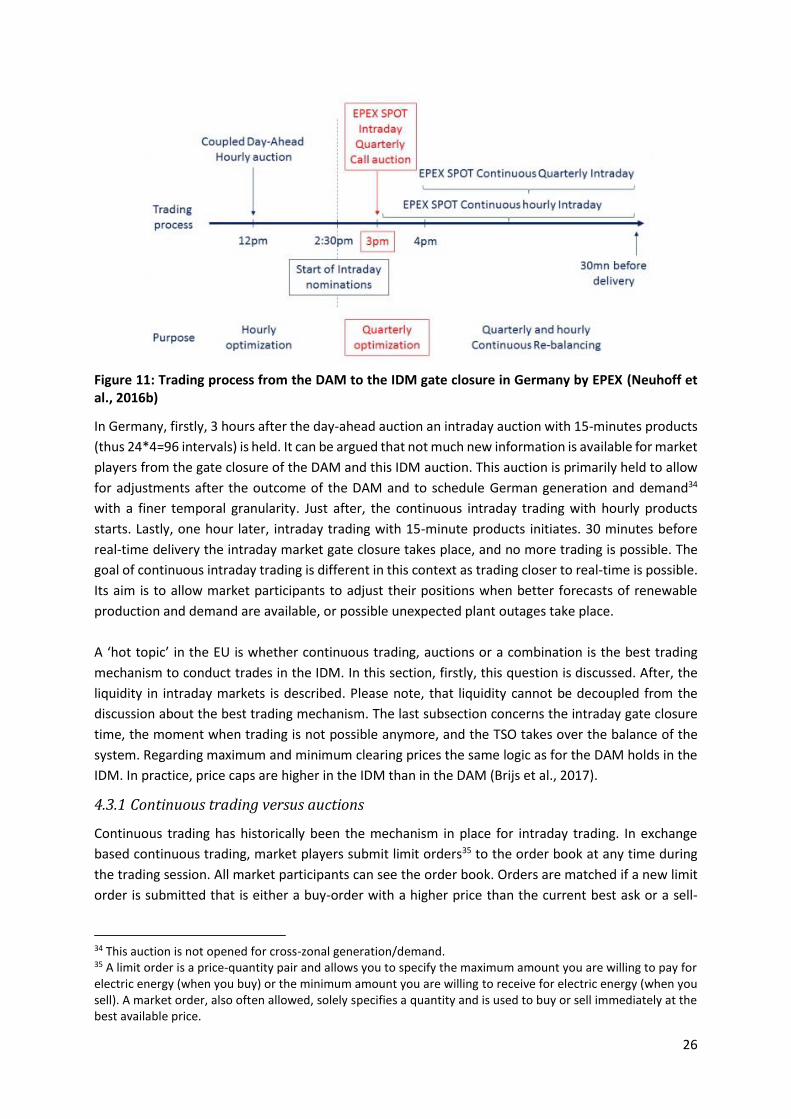
26
Figure 11: Trading process from the DAM to the IDM gate closure in Germany by EPEX (Neuhoff et al., 2016b)
In Germany, firstly, 3 hours after the day-ahead auction an intraday auction with 15-minutes products
(thus 24*4=96 intervals) is held. It can be argued that not much new information is available for market
players from the gate closure of the DAM and this IDM auction. This auction is primarily held to allow
for adjustments after the outcome of the DAM and to schedule German generation and demand34
with a finer temporal granularity. Just after, the continuous intraday trading with hourly products
starts. Lastly, one hour later, intraday trading with 15-minute products initiates. 30 minutes before
real-time delivery the intraday market gate closure takes place, and no more trading is possible. The
goal of continuous intraday trading is different in this context as trading closer to real-time is possible.
Its aim is to allow market participants to adjust their positions when better forecasts of renewable
production and demand are available, or possible unexpected plant outages take place.
A ‘hot topic’ in the EU is whether continuous trading, auctions or a combination is the best trading
mechanism to conduct trades in the IDM. In this section, firstly, this question is discussed. After, the
liquidity in intraday markets is described. Please note, that liquidity cannot be decoupled from the
discussion about the best trading mechanism. The last subsection concerns the intraday gate closure
time, the moment when trading is not possible anymore, and the TSO takes over the balance of the
system. Regarding maximum and minimum clearing prices the same logic as for the DAM holds in the
IDM. In practice, price caps are higher in the IDM than in the DAM (Brijs et al., 2017).
4.3.1 Continuous trading versus auctions
Continuous trading has historically been the mechanism in place for intraday trading. In exchange
based continuous trading, market players submit limit orders35 to the order book at any time during
the trading session. All market participants can see the order book. Orders are matched if a new limit
order is submitted that is either a buy-order with a higher price than the current best ask or a sell-
34 This auction is not opened for cross-zonal generation/demand. 35 A limit order is a price-quantity pair and allows you to specify the maximum amount you are willing to pay for electric energy (when you buy) or the minimum amount you are willing to receive for electric energy (when you sell). A market order, also often allowed, solely specifies a quantity and is used to buy or sell immediately at the best available price.

27
order with a lower price than the current best bid (Neuhoff et al., 2016b). Of the matched offers, the
initially submitted offer sets the price. This implies that buyers/sellers receive the price they bid/offer
(pay-as-bid) and that each transaction during the intraday trading session can have a different price.
This is one of the key differences with auctions, wherefore when uniform pricing is the clearing rule,
all buyers/sellers see the same price. In Box 3 the optimal clearing rule is discussed.
The CACM states that continuous trading should be in place in the intraday time frame. The matching
algorithm should be able to accommodate orders covering one market time unit and multiple market
time units (blocks). The market time unit is not specified and shall be defined by a proposal submitted
by the NEMOs (CACM, Art. 53). Next to continuous trading, complimentary regional intraday auctions
may be implemented if approved by the regulatory authorities (CACM, Art. 63). The CACM also
requires the pan-European solution based on continuous trading to be complemented by “reliable
pricing of capacity” 36 (see Section 5.2.2 for more details).
------------------------------------------------------/ Advocate/-----------------------------------------------------------------
Box 3: The optimal auction clearing rule – Marginal (or uniform) pricing vs. pay-as-bid
With continuous trading, pay-as-bid is implicitly the clearing rule used. With an auction, either pay-as-bid or uniform pricing can be opted for. In DAM auctions, marginal pricing is in place and in IDM auctions in Germany, Spain, Italy and Portugal also the marginal pricing rule is implemented. However, in the balancing market (BM) both marginal and pay-as-bid rules are employed in the EU. One paper is very frequently cited in the literature regarding this matter, namely “Uniform pricing or pay-as-bid pricing: a dilemma for California and beyond” by Kahn et al. (2001). The most important idea brought forward in the paper is that the common mistake made by people advocating that pay-as-bid pricing would lead to lower costs compared to uniform pricing is the fact that bidding strategies will be very different according to the clearing rule in place. Under pay-as-bid, the market participants would no longer have an incentive to bid their avoidable costs but instead, would base their bids anticipating the market price. This would largely remove the hoped-for savings from pay-as-bid (Littlechild, 2007). The main arguments made in favour of marginal pricing over pay-as-bid pricing are (Kahn et al., 2001; Littlechild, 2007; Müsgens et al., 2014): • Pay-as-bid introduces some inevitable reduction in efficiency as generators depart from bidding their marginal costs. Because if they solely bid their marginal cost and their bid is accepted, they won’t receive any compensation for their fixed costs or a contribution to profits. With all bids exceeding the marginal costs, by amounts that depend upon the varying estimates of the bidders of what would be the highest accepted bid, the perfect, total cost-minimizing merit order dispatch is no longer assured. • Another inefficiency inescapably introduced by pay-as-bid is the cost of forecasting market prices that it would impose on all participants. Marginal pricing rewards low costs (because all winners get the same price) whereas pay-as -bid rewards good guesses (because guesses determine the price). • There are significant economies of scale in the efforts to gather the necessary information and make such forecasts on a continuing, hour-by-hour and day-by-day basis. Under pay-as-bid,
36 In line with Article 55 of CACM, all TSOs has submitted to the National Regulatory Agencies (NRAs) a methodology for intraday capacity pricing which would introduce an auction at the intraday cross-zonal gate opening time in the European Intraday market (ENTSO-E, 2017f).
28
large players will have a better insight in bidding strategies thus having an advantage regarding the forecast of the price and will easier obtain higher prices. • There is a greater transparency of bidding under uniform pricing than under pay-as-bid facilitating attempts to detect uncompetitive behaviour. If the market were competitive, all bidders would have the incentive under uniform pricing to bid their marginal costs. Since at least marginal generating costs are relatively easily measured, it should be feasible to ascertain whether bid prices had exceeded those levels. • Under pay-as-bid no transparent price to serve as a benchmark for contract markets is available. Neuhoff et al. (2016a) argue that price reference closer to real-time is necessary. • Under pay-as-bid a supplier with market power can be successful in an auction with a bid increased beyond what would have been the bid in a competitive market. Under uniform price the monopolistically leveraged price automatically goes to all competitors alike. However, as discussed below, with marginal pricing there are also concerns when market power is present. A contra marginal pricing argument is: • Market power is the main concern when marginal pricing is applied. Namely, if there is imperfect competition and marginal pricing in place, suppliers with market power have incentives to reduce supply that could otherwise be profitably operated. The reason is that reducing supply may increase the market clearing price and thus the profitability of the infra-marginal units. An analogous strategy is not possible with pay-as-bid, because bids on one unit cannot directly influence the payments for other units. Overall, auction theory does not find a unique ranking with respect to efficiency or procurement costs regarding the settlement rules (Ausubel and Cramton, 2002). However, considering all arguments summarised in this Box, marginal pricing seems to be favoured for auctions in electricity markets.
Next to the arguments in Box 3 summing up the benefits of auctions with uniform prices, three
additional arguments in favour of auctions can be added:
1/ Allocation of cross-zonal transmission capacity (in more detail discussed in Section 5.1.1): One of the
most important arguments in favour of auctions in the IDM is the fact that soon it will be a step forward
if the IDM would be as coupled as the DAM is today. One of the issues with coupling is how to allocate
cross-zonal transmission capacity. The most efficient solution would be to hold intraday auctions which
simultaneously allocate transmission capacity (implicit allocation). Combining efficient allocation of
transmission capacity with continuous trading is not straightforward (Neuhoff et al., 2016b). With
continuous trading in place, valuable transmission capacity would be allocated on a first-come-first-
serve basis, thus possibly favouring more rapid/experienced traders instead of efficient ones. Related
to this, auctions would prevent robots capturing increasing shares of bid-ask spreads and scarcity value
of transmission capacity in the market.
2/ Liquidity (in more detail discussed in the next subsection): The (single) price obtained from an auction
increases price transparency, this is not the case with continuous trading wherefore an average or
other index needs to be computed. A liquid and transparent intraday price is beneficial especially for
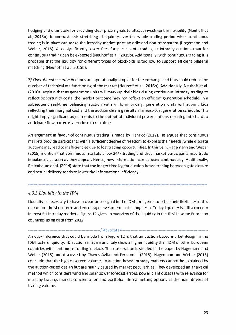
29
hedging and ultimately for providing clear price signals to attract investment in flexibility (Neuhoff et
al., 2015b). In contrast, this stretching of liquidity over the whole trading period when continuous
trading is in place can make the intraday market price volatile and non-transparent (Hagemann and
Weber, 2015). Also, significantly lower fees for participants trading at intraday auctions than for
continuous trading can be expected (Neuhoff et al., 2015b). Additionally, with continuous trading it is
probable that the liquidity for different types of block-bids is too low to support efficient bilateral
matching (Neuhoff et al., 2015b).
3/ Operational security: Auctions are operationally simpler for the exchange and thus could reduce the
number of technical malfunctioning of the market (Neuhoff et al., 2016b). Additionally, Neuhoff et al.
(2016a) explain that as generation units will mark-up their bids during continuous intraday trading to
reflect opportunity costs, the market outcome may not reflect an efficient generation schedule. In a
subsequent real-time balancing auction with uniform pricing, generation units will submit bids
reflecting their marginal cost and the auction clearing results in a least-cost generation schedule. This
might imply significant adjustments to the output of individual power stations resulting into hard to
anticipate flow patterns very close to real time.
An argument in favour of continuous trading is made by Henriot (2012). He argues that continuous
markets provide participants with a sufficient degree of freedom to express their needs, while discrete
auctions may lead to inefficiencies due to lost trading opportunities. In this vein, Hagemann and Weber
(2015) mention that continuous markets allow 24/7 trading and thus market participants may trade
imbalances as soon as they appear. Hence, new information can be used continuously. Additionally,
Bellenbaum et al. (2014) state that the longer time lag for auction-based trading between gate closure
and actual delivery tends to lower the informational efficiency.
--------------------------------------------------------------------------------------------------------------------------------------
4.3.2 Liquidity in the IDM
Liquidity is necessary to have a clear price signal in the IDM for agents to offer their flexibility in this
market on the short term and encourage investment in the long term. Today liquidity is still a concern
in most EU intraday markets. Figure 12 gives an overview of the liquidity in the IDM in some European
countries using data from 2012.
------------------------------------------------------/ Advocate/-----------------------------------------------------------------
An easy inference that could be made from Figure 12 is that an auction-based market design in the
IDM fosters liquidity. ID auctions in Spain and Italy show a higher liquidity than IDM of other European
countries with continuous trading in place. This observation is studied in the paper by Hagemann and
Weber (2015) and discussed by Chaves-Ávila and Fernandes (2015). Hagemann and Weber (2015)
conclude that the high observed volumes in auction-based intraday markets cannot be explained by
the auction-based design but are mainly caused by market peculiarities. They developed an analytical
method which considers wind and solar power forecast errors, power plant outages with relevance for
intraday trading, market concentration and portfolio internal netting options as the main drivers of
trading volume.
30
Figure 12: Intraday markets in selected European countries with 2012 data (Hagemann and Weber, 2015)
Next to these fundamental drivers, one of the most important reasons found for the high liquidity in
the Italian, Spanish and Portuguese market was that rescheduling of generation output between
power plants within one generation portfolio is only possible via trades in the intraday market. No
bilateral trade after the DAM and internal portfolio netting outside of the market are allowed (Rodilla
and Batlle, 2015). Additionally, Hagemann and Weber (2015) also argue that renewable support
schemes have an influence on IDM liquidity. In countries with low-risk support schemes, such as a feed-
in tariff (FIT), the balancing responsibility is typically carried over to the TSO (or DSO). TSOs need to
trade imbalances on the intraday markets, raising the trading volume. On the contrary, in countries
with high-risk support schemes, such as feed-in premiums (FIP), the owners of vRES are responsible
for their forecast errors. These, in contrary to the TSO, can either use controllable generation for
internal self-balancing or do not manage forecast errors actively in the intraday market if they are too
small.
Chaves-Ávila and Fernandes (2015) and Rodilla and Batlle (2015) also mention three other reasons
explaining the high liquidity in the Spanish market. Firstly, there is an additional upward regulation
reserve, which can be called upon, consisting of units which were not dispatched in the DAM. If a unit
gets selected in this market, it is forced to bid into the IDM in order to get committed. Also, there is a
national coal support mechanism which has given incentives to some units to avoid being committed
in the DAM and bidding in the IDM instead. And lastly, price arbitrage opportunities were identified
between DAM and IDM the last years. These might have been (partly) caused by the regulation around
this upward reserve and the national coal support scheme.
In December 2014, an auction with 15-min products was also introduced in Germany (Figure 11). It is
observed by Neuhoff et al. (2016b) that the implementation of this auction led to increased liquidity.
They find that traded intraday volumes with 10-15 GWh have been much higher than with continuous
trading alone that rarely cleared more than 5 GWh. In contrast with Hagemann and Weber (2015) and
31
Chaves-Ávila and Fernandes (2015), Neuhoff et al. (2016b) do not attribute the high liquidity levels to
market peculiarities, but more clearly argue in favour of intraday auctions over continuous trading in
the IDM.
Not yet mentioned in this discussion but extremely important regarding this matter is the fact that the
high enough imbalance settlements, to be paid when being unbalanced in real-time, should give an
incentive for agents to balance their output on the IDM. If these price signals are not strong enough,
agents will not feel the need to trade on the IDM and liquidity will remain low. Additionally, it is
necessary for vRES to be held responsible (preferably under the same rules as conventional units) for
their imbalances, as such they are forced to trade in the IDM. Also, transparent “near-real-time”
information about the system state is of crucial importance concerning this matter. If agents have this
information, they can estimate potential imbalance settlements and they will be strongly incentivized
to balance their positions in the IDM, especially when it is highly needed from a system perspective. A
proper functioning liquid IDM is very dependent upon well-designed balancing settlements and rules.
--------------------------------------------------------------------------------------------------------------------------------------
4.3.3 IDM gate closure: the gap between trading and real-time operation
As implicitly stated in Article 59 (2) of the CACM, the length of the IDM gate closure is a trade-off
between:
‘’(a) a maximisation of market participants' opportunities for adjusting their balances by trading in the
intraday market time- frame as close as possible to real time;
and (b) providing TSOs and market participants with sufficient time for their scheduling and balancing
processes in relation to network and operational security.’’
Further, it is stated in the CACM that the intraday cross-zonal gate closure time, the gate closure time
for cross-zonal transmission capacity, shall be at most one hour before real-time (CAMC, Art. 59(3)).
Intraday energy trading for a given market unit for a bidding zone border shall be allowed until the
intraday cross-zonal gate closure time (CAMC, Art. 59(4)).
The closer gate closure to real-time, the better vRES will be able to update their forecast and the more
they will be trading in the IDM to avoid imbalances (if imbalance settlements give the required
incentive to adjust). A gate closure closer to real time will lead to a higher liquidity in the intraday
market and a better deployment of flexible resources, the only resources, next to (fast) demand
response (DR), that are able to adjust their output close to real time. Because of a more accurate
dispatch of flexible peak units, fewer power plants will have to operate (inefficiently) at partial load in
order to deliver balancing services (Müsgens and Neuhoff, 2006). Also, less reserve power capacity
will need to be contracted, and less real-time action of the SO will be required, this all leading to a
lower system cost.
The main reason why there is a time lag between gate closure and real-time is the fact that grid
operators require sufficient time after the closure of trades to check system stability and take any
necessary measures before real time. The level of coordination between TSOs and power exchanges
will become increasingly important to minimise the gap between gate close and real time.
32
Matching markets with grids: redispatch and countertrading
In Europe, zonal pricing is applied as described in Section 2.1. Shortly, this means that electricity is
traded in a bidding zone which is linked to other bidding zones. The physical network within a bidding
zone is seen as a copper plate (no network constraints), while the links between bidding zones are
taken into account when trading. If cross-zonal links are congested between the bidding zones, the
respective markets are ‘split’; if not, the markets are ‘coupled’. Coupled markets imply the aggregation
of supply and demand curves for the coupled zones when clearing the market.
Now, not incorporating grid constraints within bidding zones is a serious simplification. The flows
resulting from electricity trading does not always lead to feasible flows through all lines within a
bidding zone (internal congestion). Lately, internal congestion is a structural problem in several regions
in Europe, mainly due to the increase in renewable generation and more volatile cross-border trade
(ACER and ENTSOE, 2012; Dijk and Willems, 2011; Kunz and Zerrahn, 2016; Van den Bergh et al., 2015).
In the short run, network congestion can be relieved by non-costly preventive measures, such as
changing grid topology or by costlier curative measures, such as countertrading or redispatch. With
countertrading or redispatch, the TSO arranges an increase in generation at one end of the congested
grid area, compensated by a decrease at the other end. The costs of these deviations from the spot
market dispatch are socialised through network tariffs (Kunz and Zerrahn, 2016). If countertrading or
redispatch is not available, TSOs may curtail previously allocated cross-border capacities. In that case,
the owners of transmission rights have to be compensated.
Definitions of countertrading and redispatch are found in a presentation by ACER and ENTSOE (2012):
• Redispatch: “Any measure activated by one or several system operators by altering the generation and/or load pattern in order to change physical flows in the Transmission System and relieve a physical congestion. The precise generation or load pattern alteration is pre-defined.” Redispatching can be:
o Internal redispatching: the redispatching is performed in the bidding zone where the congestion is.
o External redispatching: the redispatching is performed in bidding zone A whereas the congestion is on bidding zone B.
o Cross-border redispatching: the redispatching is carried out in different bidding zones
• Countertrading: “Cross zonal energy exchange initiated by system operators between two bidding zones to relieve a physical congestion. The precise generation or load pattern alteration is not pre-defined.”
In the CACM, Article 35(5) it is stated that the pricing of redispatch and countertrading shall be based
on:
‘’(a) prices in the relevant electricity markets for the relevant time frame; or
(b) costs of redispatching and/or countertrading resources calculated transparently on the basis of incurred costs.’’
ACER/CEER (2016) reports that the remuneration of activated internal or cross-zonal re-dispatching
33
differs among Member States. It is found that the most common method used is the pay-as-bid pricing
followed by the regulated pricing based on either a market price (e.g. DA price) or a cost-based pricing
(e.g. remuneration for the cost of fuel and other costs related to the change in the operating schedule
of the plant).
------------------------------------------------------/ Advocate/-----------------------------------------------------------------
Redispatch and countertrading are short-term solutions to solve internal congestion. In the long run,
the TSO can build new lines to accommodate the flow patterns. Alternatively, bidding zones can be
redrawn or nodal electricity markets can be introduced. Nodal pricing is applied in some regions of the
US (e.g. PJM) and can be considered as an extreme form of zonal pricing, namely each node in the
transmission network becomes a bidding zone. Dijk and Willems (2011) explain that “under nodal spot
pricing, electricity prices reflect physical constraints, and hence, scarcity of the transmission network.
In the short run, nodal spot prices, therefore, ensure optimal usage of the transmission network. Over
the long term, they give the optimal incentives for new investments.”
None of these three solutions is without downsides. Building new transmission lines cost time, just as
redrawing bidding zones do, and nodal pricing is not in line with the European target model for many
reasons.
Lastly, it is generally agreed upon that closer cooperation in congestion management between TSOs
has a beneficial impact. More specifically, the sharing of network and dispatch information, cross-
border counter-trading, and multilateral redispatch can reduce overall system costs and allow for more
cross-zonal capacity to be offered to the market (ACER and ENTSOE, 2012; Kunz and Zerrahn, 2016).
For that reason, the CACM (Article 35) strongly advocates more coordinated remedial actions, in
particular for cross-border relevance. For example, TSOs, at least within a capacity calculation region,
shall agree on a common redispatching and/or countertrading arrangements. Also, in Article 74 is
described that a redispatch and countertrading cost-sharing methodology will be developed as
coordinated remedial actions can have distributional effects.
--------------------------------------------------------------------------------------------------------------------------------------
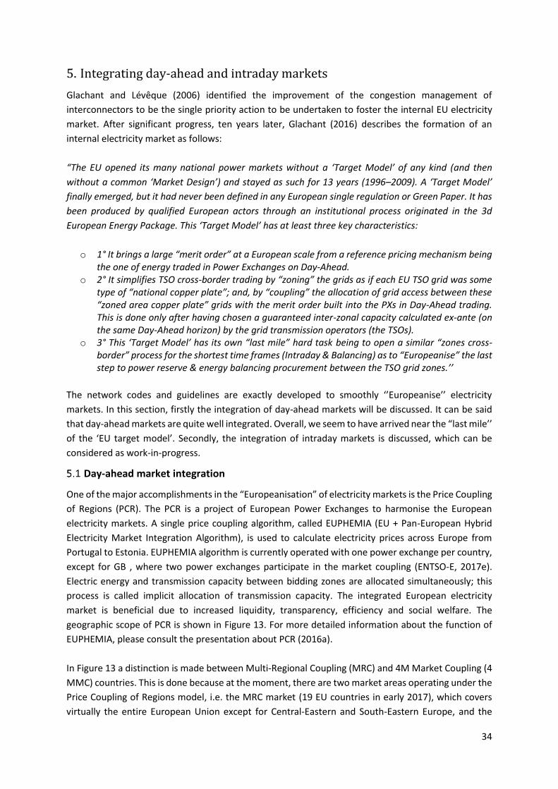
34
5. Integrating day-ahead and intraday markets
Glachant and Lévêque (2006) identified the improvement of the congestion management of
interconnectors to be the single priority action to be undertaken to foster the internal EU electricity
market. After significant progress, ten years later, Glachant (2016) describes the formation of an
internal electricity market as follows:
“The EU opened its many national power markets without a ‘Target Model’ of any kind (and then
without a common ‘Market Design’) and stayed as such for 13 years (1996–2009). A ‘Target Model’
finally emerged, but it had never been defined in any European single regulation or Green Paper. It has
been produced by qualified European actors through an institutional process originated in the 3d
European Energy Package. This ‘Target Model’ has at least three key characteristics:
o 1° It brings a large “merit order” at a European scale from a reference pricing mechanism being the one of energy traded in Power Exchanges on Day-Ahead.
o 2° It simplifies TSO cross-border trading by “zoning” the grids as if each EU TSO grid was some type of “national copper plate”; and, by “coupling” the allocation of grid access between these “zoned area copper plate” grids with the merit order built into the PXs in Day-Ahead trading. This is done only after having chosen a guaranteed inter-zonal capacity calculated ex-ante (on the same Day-Ahead horizon) by the grid transmission operators (the TSOs).
o 3° This ‘Target Model’ has its own “last mile” hard task being to open a similar “zones cross-border” process for the shortest time frames (Intraday & Balancing) as to “Europeanise” the last step to power reserve & energy balancing procurement between the TSO grid zones.’’
The network codes and guidelines are exactly developed to smoothly ‘’Europeanise’’ electricity
markets. In this section, firstly the integration of day-ahead markets will be discussed. It can be said
that day-ahead markets are quite well integrated. Overall, we seem to have arrived near the “last mile’’
of the ‘EU target model’. Secondly, the integration of intraday markets is discussed, which can be
considered as work-in-progress.
Day-ahead market integration
One of the major accomplishments in the “Europeanisation” of electricity markets is the Price Coupling
of Regions (PCR). The PCR is a project of European Power Exchanges to harmonise the European
electricity markets. A single price coupling algorithm, called EUPHEMIA (EU + Pan-European Hybrid
Electricity Market Integration Algorithm), is used to calculate electricity prices across Europe from
Portugal to Estonia. EUPHEMIA algorithm is currently operated with one power exchange per country,
except for GB , where two power exchanges participate in the market coupling (ENTSO-E, 2017e).
Electric energy and transmission capacity between bidding zones are allocated simultaneously; this
process is called implicit allocation of transmission capacity. The integrated European electricity
market is beneficial due to increased liquidity, transparency, efficiency and social welfare. The
geographic scope of PCR is shown in Figure 13. For more detailed information about the function of
EUPHEMIA, please consult the presentation about PCR (2016a).
In Figure 13 a distinction is made between Multi-Regional Coupling (MRC) and 4M Market Coupling (4
MMC) countries. This is done because at the moment, there are two market areas operating under the
Price Coupling of Regions model, i.e. the MRC market (19 EU countries in early 2017), which covers
virtually the entire European Union except for Central-Eastern and South-Eastern Europe, and the
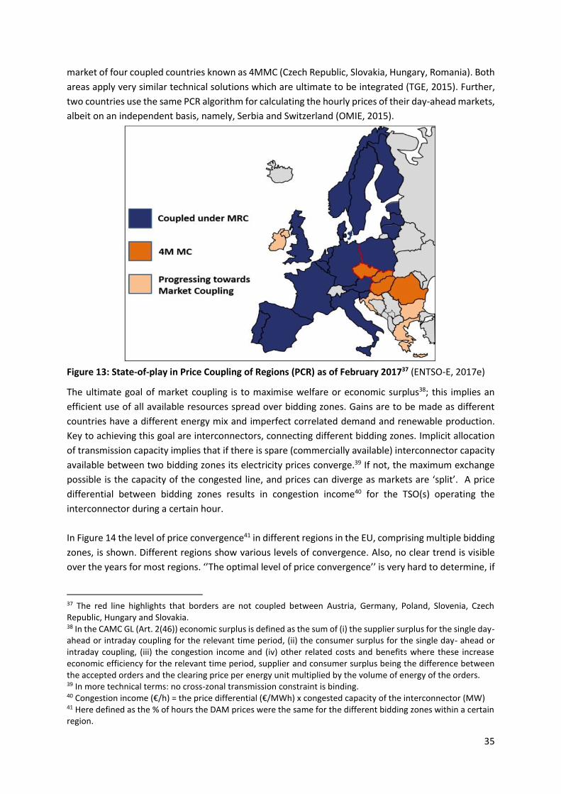
35
market of four coupled countries known as 4MMC (Czech Republic, Slovakia, Hungary, Romania). Both
areas apply very similar technical solutions which are ultimate to be integrated (TGE, 2015). Further,
two countries use the same PCR algorithm for calculating the hourly prices of their day-ahead markets,
albeit on an independent basis, namely, Serbia and Switzerland (OMIE, 2015).
Figure 13: State-of-play in Price Coupling of Regions (PCR) as of February 201737 (ENTSO-E, 2017e)
The ultimate goal of market coupling is to maximise welfare or economic surplus38; this implies an
efficient use of all available resources spread over bidding zones. Gains are to be made as different
countries have a different energy mix and imperfect correlated demand and renewable production.
Key to achieving this goal are interconnectors, connecting different bidding zones. Implicit allocation
of transmission capacity implies that if there is spare (commercially available) interconnector capacity
available between two bidding zones its electricity prices converge.39 If not, the maximum exchange
possible is the capacity of the congested line, and prices can diverge as markets are ‘split’. A price
differential between bidding zones results in congestion income40 for the TSO(s) operating the
interconnector during a certain hour.
In Figure 14 the level of price convergence41 in different regions in the EU, comprising multiple bidding
zones, is shown. Different regions show various levels of convergence. Also, no clear trend is visible
over the years for most regions. ‘’The optimal level of price convergence’’ is very hard to determine, if
37 The red line highlights that borders are not coupled between Austria, Germany, Poland, Slovenia, Czech Republic, Hungary and Slovakia. 38 In the CAMC GL (Art. 2(46)) economic surplus is defined as the sum of (i) the supplier surplus for the single day-ahead or intraday coupling for the relevant time period, (ii) the consumer surplus for the single day- ahead or intraday coupling, (iii) the congestion income and (iv) other related costs and benefits where these increase economic efficiency for the relevant time period, supplier and consumer surplus being the difference between the accepted orders and the clearing price per energy unit multiplied by the volume of energy of the orders. 39 In more technical terms: no cross-zonal transmission constraint is binding. 40 Congestion income (€/h) = the price differential (€/MWh) x congested capacity of the interconnector (MW) 41 Here defined as the % of hours the DAM prices were the same for the different bidding zones within a certain region.
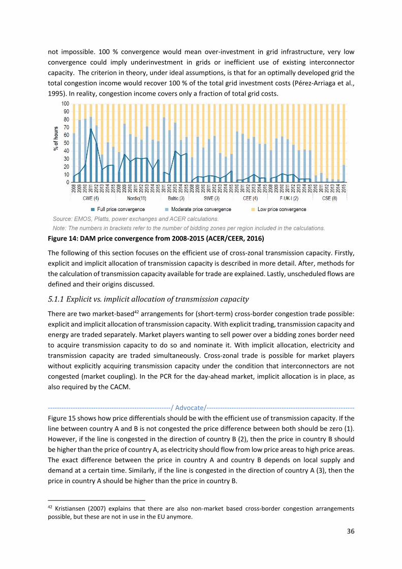
36
not impossible. 100 % convergence would mean over-investment in grid infrastructure, very low
convergence could imply underinvestment in grids or inefficient use of existing interconnector
capacity. The criterion in theory, under ideal assumptions, is that for an optimally developed grid the
total congestion income would recover 100 % of the total grid investment costs (Pérez-Arriaga et al.,
1995). In reality, congestion income covers only a fraction of total grid costs.
Figure 14: DAM price convergence from 2008-2015 (ACER/CEER, 2016)
The following of this section focuses on the efficient use of cross-zonal transmission capacity. Firstly,
explicit and implicit allocation of transmission capacity is described in more detail. After, methods for
the calculation of transmission capacity available for trade are explained. Lastly, unscheduled flows are
defined and their origins discussed.
5.1.1 Explicit vs. implicit allocation of transmission capacity
There are two market-based42 arrangements for (short-term) cross-border congestion trade possible:
explicit and implicit allocation of transmission capacity. With explicit trading, transmission capacity and
energy are traded separately. Market players wanting to sell power over a bidding zones border need
to acquire transmission capacity to do so and nominate it. With implicit allocation, electricity and
transmission capacity are traded simultaneously. Cross-zonal trade is possible for market players
without explicitly acquiring transmission capacity under the condition that interconnectors are not
congested (market coupling). In the PCR for the day-ahead market, implicit allocation is in place, as
also required by the CACM.
------------------------------------------------------/ Advocate/-----------------------------------------------------------------
Figure 15 shows how price differentials should be with the efficient use of transmission capacity. If the
line between country A and B is not congested the price difference between both should be zero (1).
However, if the line is congested in the direction of country B (2), then the price in country B should
be higher than the price of country A, as electricity should flow from low price areas to high price areas.
The exact difference between the price in country A and country B depends on local supply and
demand at a certain time. Similarly, if the line is congested in the direction of country A (3), then the
price in country A should be higher than the price in country B.
42 Kristiansen (2007) explains that there are also non-market based cross-border congestion arrangements possible, but these are not in use in the EU anymore.

37
Figure 15: Zonal pricing and optimal cross-zonal allocation (FSR, 2014)
Now, under ideal assumptions, the outcome for explicit allocation and implicit allocation should be the
same and optimal (as shown in Figure 15). In Figure 16, results are shown for the French-Spanish
border in 2012. Explicit auctions for cross-zonal transmission were held, PCR was not yet in place. The
pattern diverges quite strongly from what we would expect with optimal cross-zonal allocation. In
some cases, the prices differ between the countries while the interconnector is not congested. Even
more extreme, often the price in France was higher, but the electricity was flowing towards Spain
(quadrant 1) or vice-versa (quadrant 3). Reasons for the deviation from optimal usage are coordination
issues (timing, limited information, imperfect forecast) for agents or possibly uncompetitive behaviour.
Figure 16: Explicit cross-zonal allocation: use of net daily capacities on the French-Spanish interconnector compared with hourly DAM price differences, data of 2012 (FSR, 2014)
Figure 17 shows the results for implicit allocation between Belgium and France in 2012. These markets
were coupled at the time. It can be seen that with implicit allocation cross-zonal capacity is efficiently
used. With implicit allocation, there are no coordination issues.

38
Figure 17: Implicit cross-zonal allocation : use of net daily capacities on the France-Belgium interconnector compared with hourly price differences, data of 2012 (FSR, 2014)
--------------------------------------------------------------------------------------------------------------------------------------
Efficient allocation of available cross-zonal transmission capacity is one important dimension of well-
functioning integrated electricity markets. Another crucial dimension is the calculation of the total
transmission capacity that should be allocated to market players. In other words, in this subsection, it
was discussed how to efficiently allocate cross-border capacity, while in the next subsection, the
questions ‘’how much cross-zonal capacity should be available for trade without putting the system at
risk?’’ is tackled. Limited available capacity for trade, even when efficiently allocated, does not lead to
fully integrated markets.
5.1.2 Cross-zonal capacity calculation: issues and approaches
It is not straightforward to properly calculate the available transmission capacity between bidding
zones. The reason for this is that electricity doesn’t flow directly from generators to consumers, but
spreads out over a (meshed AC) network according to the laws of physics (Kirchhoff laws). Energy flows
across all paths in proportion to their admittance. This implies that one line can be constrained by
other lines before reaching its maximal thermal capacity.43 Several other issues, directly or indirectly
related to the physical nature of electricity and zonal pricing, make it impossible to fully offer the
thermal capacity of lines for trade (Nabe and Neuhoff (2015), Schavemaker and Beune (2013) and Van
den Bergh et al. (2016)):
• Calculating cross-zonal capacity for trade is a chicken-and-egg-issue. Namely, the transmission capacity available for commercial transactions between pricing zones depends on the generation and load pattern within a bidding zone. However, the generation and load pattern within a bidding zone is a function of the market outcome and as such is influenced by the volume of transmission capacity made available by TSOs for cross-zonal trade. This implies that safety margins need to be introduced to compensate for approximations and simplifications made.
43 For an illustrative example please see Section 6.1.3 (The Transmission Grid: Technical Considerations) of Pérez-Arriaga (2013).
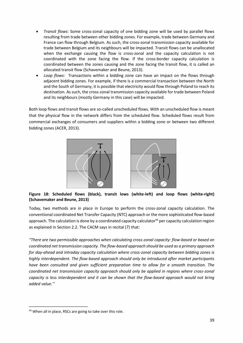
39
• Transit flows: Some cross-zonal capacity of one bidding zone will be used by parallel flows resulting from trade between other bidding zones. For example, trade between Germany and France can flow through Belgium. As such, the cross-zonal transmission capacity available for trade between Belgium and its neighbours will be impacted. Transit flows can be unallocated when the exchange causing the flow is cross-zonal and the capacity calculation is not coordinated with the zone facing the flow. If the cross-border capacity calculation is coordinated between the zones causing and the zone facing the transit flow, it is called an allocated transit flow (Schavemaker and Beune, 2013).
• Loop flows: Transactions within a bidding zone can have an impact on the flows through adjacent bidding zones. For example, if there is a commercial transaction between the North and the South of Germany, it is possible that electricity would flow through Poland to reach its destination. As such, the cross-zonal transmission capacity available for trade between Poland and its neighbours (mostly Germany in this case) will be impacted.
Both loop flows and transit flows are so-called unscheduled flows. With an unscheduled flow is meant
that the physical flow in the network differs from the scheduled flow. Scheduled flows result from
commercial exchanges of consumers and suppliers within a bidding zone or between two different
bidding zones (ACER, 2013).
Figure 18: Scheduled flows (black), transit lows (white-left) and loop flows (white-right) (Schavemaker and Beune, 2013)
Today, two methods are in place in Europe to perform the cross-zonal capacity calculation. The
conventional coordinated Net Transfer Capacity (NTC) approach or the more sophisticated flow-based
approach. The calculation is done by a coordinated capacity calculator44 per capacity calculation region
as explained in Section 2.2. The CACM says in recital (7) that:
“There are two permissible approaches when calculating cross-zonal capacity: flow-based or based on
coordinated net transmission capacity. The flow-based approach should be used as a primary approach
for day-ahead and intraday capacity calculation where cross-zonal capacity between bidding zones is
highly interdependent. The flow-based approach should only be introduced after market participants
have been consulted and given sufficient preparation time to allow for a smooth transition. The
coordinated net transmission capacity approach should only be applied in regions where cross-zonal
capacity is less interdependent and it can be shown that the flow-based approach would not bring
added value.’’
44 When all in place, RSCs are going to take over this role.

40
Further, in Article 20(2) of CAMC is stated that ‘’no later than 10 months after the approval of the
proposal for a capacity calculation region in accordance with Article 15(1), all TSOs in each capacity
calculation region shall submit a proposal for a common coordinated capacity calculation methodology
within the respective region.’’ A methodology for both day-ahead and intraday capacity calculation
shall be proposed. Some delay was allowed for certain CCRs (CACM, Art. 20(3,4)). In the summer of
2017, the TSOs representing the CCRs Hansa, CORE, Nordic, Channel, SWE and IU submitted a proposal
for common coordinated capacity calculation methodology within the respective region. See Figure 4
(left) for a depiction of these CCRs. After, the idea is that the capacity calculation of two or more
adjacent CCRs in the same synchronous area shall be integrated if all CCRs implement a flow-based
capacity calculation methodology (CACM, Art. 20(5)).
In the following of the Subsection, first, the conventional NTC approach is explained. After, the flow-
based approach is described. Lastly, a mapping between the issues with capacity calculation and
possible remedies is done.
------------------------------------------------------/ Advocate/-----------------------------------------------------------------
Coordinated Net Transfer Capacity (NTC) approach
In the literature, the approach to calculate NTC values is denominated the Available Transfer Capacity
(ATC) approach (Plancke et al., 2016; Van den Bergh et al., 2016). Van den Bergh et al. (2016) explain
that in the ATC approach the link between the physical network and commercial transactions is
strongly simplified. Bidding zones are represented by one equivalent node, and only cross-zonal links
are considered as shown in Figure 19 (left) for three bidding zones.
Figure 19: Grid model under the ATC approach (left) and flow domain (right) (Van den Bergh et al., 2016)
With ATC, the cross-zonal capacity offered for one link (the so-called NTC value) is independent of the
flows on other cross-zonal links as can be seen in Figure 19 (right). TSOs use a heuristic to calculate the
cross-zonal capacity available for trade based on assumptions of the market outcome (2-days ahead)
and associated physical flows. As such, capacity allocation takes place ex-ante, completely separated,
from the market clearing.
Today, the ATC approach is used in European markets, except for Central-West Europe, where flow-
based market coupling was introduced in May 2015 (ACER/CEER, 2016). This approach is compatible
with both explicit and implicit allocation of transmission capacity. Van den Bergh et al. (2016) add:
“given the strong assumptions inherent to the ATC method, the ATC value needs to be conservative to
avoid overloading physical lines.”
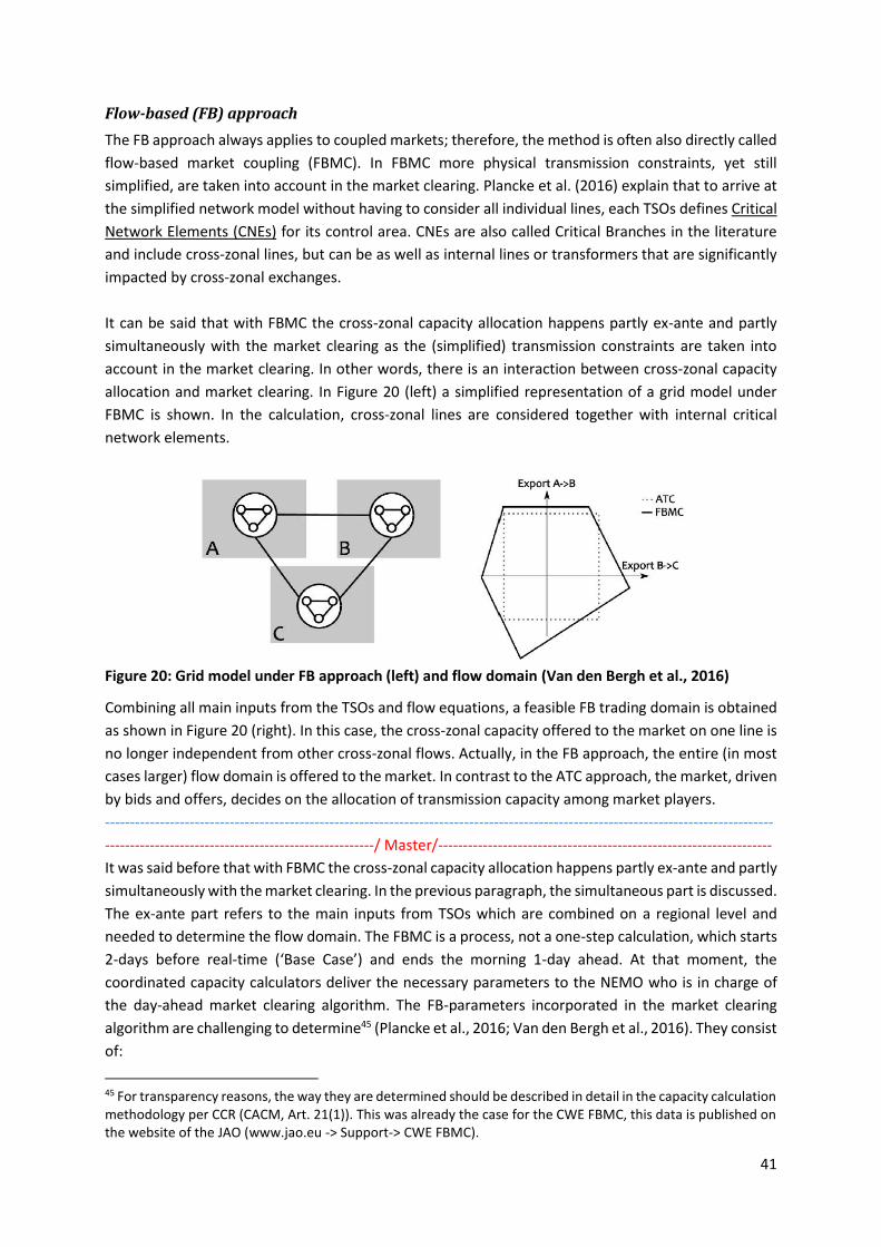
41
Flow-based (FB) approach
The FB approach always applies to coupled markets; therefore, the method is often also directly called
flow-based market coupling (FBMC). In FBMC more physical transmission constraints, yet still
simplified, are taken into account in the market clearing. Plancke et al. (2016) explain that to arrive at
the simplified network model without having to consider all individual lines, each TSOs defines Critical
Network Elements (CNEs) for its control area. CNEs are also called Critical Branches in the literature
and include cross-zonal lines, but can be as well as internal lines or transformers that are significantly
impacted by cross-zonal exchanges.
It can be said that with FBMC the cross-zonal capacity allocation happens partly ex-ante and partly
simultaneously with the market clearing as the (simplified) transmission constraints are taken into
account in the market clearing. In other words, there is an interaction between cross-zonal capacity
allocation and market clearing. In Figure 20 (left) a simplified representation of a grid model under
FBMC is shown. In the calculation, cross-zonal lines are considered together with internal critical
network elements.
Figure 20: Grid model under FB approach (left) and flow domain (Van den Bergh et al., 2016)
Combining all main inputs from the TSOs and flow equations, a feasible FB trading domain is obtained
as shown in Figure 20 (right). In this case, the cross-zonal capacity offered to the market on one line is
no longer independent from other cross-zonal flows. Actually, in the FB approach, the entire (in most
cases larger) flow domain is offered to the market. In contrast to the ATC approach, the market, driven
by bids and offers, decides on the allocation of transmission capacity among market players.
--------------------------------------------------------------------------------------------------------------------------------------
------------------------------------------------------/ Master/-------------------------------------------------------------------
It was said before that with FBMC the cross-zonal capacity allocation happens partly ex-ante and partly
simultaneously with the market clearing. In the previous paragraph, the simultaneous part is discussed.
The ex-ante part refers to the main inputs from TSOs which are combined on a regional level and
needed to determine the flow domain. The FBMC is a process, not a one-step calculation, which starts
2-days before real-time (‘Base Case’) and ends the morning 1-day ahead. At that moment, the
coordinated capacity calculators deliver the necessary parameters to the NEMO who is in charge of
the day-ahead market clearing algorithm. The FB-parameters incorporated in the market clearing
algorithm are challenging to determine45 (Plancke et al., 2016; Van den Bergh et al., 2016). They consist
of:
45 For transparency reasons, the way they are determined should be described in detail in the capacity calculation methodology per CCR (CACM, Art. 21(1)). This was already the case for the CWE FBMC, this data is published on the website of the JAO (www.jao.eu -> Support-> CWE FBMC).

42
• Zonal Power Transfer Distribution Factors (PTDFs): o What? Zonal PTDFs describe the linear relationship between the physical flow in a
critical branch and the net exchange position46 of a specific bidding zone. They are formulated in a (sparse) matrix form with on one dimension all the bidding zones and on the other dimension all the cross-zonal interconnectors.
o How are they derived? With zonal pricing nodes are grouped per zone, this implies that in order to correctly represent flows between zones, zonal PTDFs need to be approximated from what happens at nodal level within a zone. Generation Shift Keys (GSKs) ‘translate’ changes in generation/consumption at nodal level to impacts on the net exchange level of a zone. GSKs are not easy to determine as they are based on predictions of the market outcome and subject to forecast errors. Each TSO calculates the GSKs for his control area. Van den Bergh et al. (2016) describe that the way TSOs derived GSKs in the past was not harmonised. The CAMC GL demands in Article 24 that the common capacity calculation methodology (per capacity calculation regions) shall include a proposal for a methodology to determine a common way to derive generation shift keys for each bidding zone. Additionally, also the common grid model plays a crucial role in obtaining optimal forecast to increase the accuracy of GSKs.
• Available Margins (AM) on Critical Network elements (CNE): o What? The AM is the maximal flow (a fraction of the thermal limit) that can be endured
by CNEs due to flows induced by day-ahead trade. In the literature, the Available Margin is also referred to as the Remaining Available Margin (RAM).
o How are they derived? The determination of 1.) what the critical network elements are within a control zone and 2.) the contingencies (critical outages) to be considered for system security are key for the determination of this FB-parameter. Van den Bergh et al. (2016) find that the exact method to derive the AM is confusing and inconsistently formulated in consulted FBMC reports. In general, AM are derived as the maximal flow an element can hold minus 3 flows:
▪ The Reference Flow on a CNE: the reference flow is caused by transactions between or within bidding zones out of the Day-ahead market, such bilateral transactions or transactions in forward markets.
▪ A Final Adjustment value: a margin which is TSO specific and depends on, for example, complex remedial actions. For the determination of this value it is important to ensure that there is no discrimination between internal and cross-zonal flows (CACM, Art. 29(7)(d)).
▪ A Flow Reliability Margin: a safety margin compensating for approximations made in the FB-approach
Also, regarding the calculation of the AM and its components, the CACM tends to create transparency and harmonisation with Article 29.
--------------------------------------------------------------------------------------------------------------------------------------
------------------------------------------------------/ Advocate/-----------------------------------------------------------------
Van den Bergh et al. (2016) state that by better representation of the physical characteristics with the
FB approach, the cross-zonal capacity offered to the market can be determined in a less conservative
way. Plancke et al. (2016) agree that the FB is more sophisticated than the ATC approach, resulting in
(theoretically) higher cross-zonal capacity to be offered to the market. However, the authors add that
operational challenges could arise due to the increased complexity.
46 The net exchange position of a bidding zone equals to the total production within the zone minus the total consumption within a zone. If the production is higher than the consumption, the zone will be a net exporter. Vice-versa the zone would be a net importer.

43
Limited commercial cross-zonal capacity: causes and issues
ACER/CEER (2016) finds in its Market Monitoring report that, in recent years, the volume of tradable
cross-zonal capacities in the EU has remained relatively limited. Improvement was anticipated as
investments in the transmission networks took place and some improvements in capacity calculation
methods were implemented. On most EU borders, only a small part of the physical capacities is offered
to the market and that there are important variations between regions. Their analysis shows that on
average 84% of HVDC and 28% of HVAC interconnector’s physical capacity is used for trading.
A first reason described in ACER/CEER (2016) which could explain the low utilisation rates of cross-
zonal capacity is a lack of coordination between TSOs concerning the cross-zonal capacity calculation.
On 40 out of 48 assessed borders, either a bilateral or partly coordinated capacity calculation method
is applied. Additionally, on many borders during certain market time frames, capacity calculation is
simply not applied by at least one of the TSOs. The CACM is tackling this issue by the determination of
coordinated capacity regions (CACM, Art. 15(1)) and demanding a common capacity calculation
methodology per CCR (Art. 20(2)). Also, by 31 December 2020, all regions shall use a harmonised
capacity calculation methodology, which is described in more details in Article 21(4) of the CACM.
A second reason explaining the low utilisation rates of cross-zonal transmission capacity, stated in the
same report, is the controversial claim that due to the lack of correct and adequate incentives for TSOs,
the latter prefer, during the capacity calculation process, to limit ex-ante cross-zonal capacities in order
to limit the costs of redispatching and countertrading required to accommodate internal flows. It is
hard to show that TSOs demonstrate such behaviour. Glachant and Pignon (2005) demonstrate, using
a theoretical example, that such behaviour could be both feasible and would necessitate only a slight
manipulation of the data. In the CACM, it is clearly stated that internal and cross-border flows should
be treated equally. More precisely, it is stated that there should be no undue discrimination between
internal and cross-zonal flows. In Article 23 of the CACM47 it is written that:
(1) Each TSO shall respect the operational security limits and contingencies used in operational security
analysis.
(2) If the operational security limits and contingencies used in capacity calculation are not the same as
those used in operational security analysis, TSOs shall describe in the proposal for the common capacity
calculation methodology the particular method and criteria they have used to determine the
operational security limits and contingencies used for capacity calculation.
--------------------------------------------------------------------------------------------------------------------------------------
47 ACER (2016) repeats point 3 of Article 23 of CACM in their recommendation on the common capacity calculation and redispatch and countertrading cost sharing methodologies to not take into account internal congestion when calculating cross-zonal capacity (it should in principle be resolved with remedial actions in the short term and other solutions in the long term), excepted temporarily, if: (a) needed to ensure operational security; and (b) economically more efficient than other available remedies (taking into account the EU-wide welfare effects of the reduction of cross-zonal capacity) and minimises the negative impacts on the internal market in electricity.

44
(3) If TSOs apply allocation constraints48, they can only be determined using:
(a) constraints that are needed to maintain the transmission system within operational
security limits and that cannot be transformed efficiently into maximum flows on critical
network elements; or
(b) constraints intended to increase the economic surplus for single day-ahead or intraday
coupling.
Next to increased coordination between TSOs and equal treatment of internal and cross-zonal flows,
there are other issues directly related to zonal pricing, the choice made in the EU Target Model.49
Intraday market integration
The Target Model for the intraday market has been laid down in the CACM and is based on continuous
trading where cross-zonal transmission capacity is allocated through implicit continuous allocation.
Implicit allocation implies that the common IT system will accommodate the continuous matching of
bids and orders from market participants in one bidding zone with bids and orders coming from its
own bidding zone and from any other bidding zone while cross-zonal capacity is still available. By
integrating intraday markets, the possibility for market parties to trade close to real-time can be
significantly improved as they also can benefit from the available liquidity in other zones next to their
bidding zone. This initiative is called the Cross-Border Intraday Market Project (XBID). Currently, the
XBID project is comprised of members from 14 European countries as illustrated in Figure 21. Accession
countries are future members of the XBID project. The complex XBID project is work-in-progress and
plans to go live by the end of the third quarter of 2017 (ENTSO-E, 2017e).
XBID will support not only implicit continuous intraday trading but also explicit intraday cross-border
allocation. Both are in line with the CACM, as Article 64 says that:
“Where jointly requested by the regulatory authorities of the Member States of each of the bidding
zone borders concerned, the TSOs concerned shall also provide explicit allocation, in addition to implicit
allocation, that is to say, capacity allocation separate from the electricity trade, via the capacity
management module on bidding zone borders.”
However, explicit allocation of cross-zonal transmission capacity is only transitory as implied by Article
65, titled ‘Removal of explicit allocation’. More precisely:
‘’The NEMOs concerned shall cooperate closely with the TSOs concerned and shall consult market
participants in order to translate the needs of market participants linked to explicit capacity allocation
rights into non-standard intraday products50.’’
48 Defined in the CACM (Art. 2(6)) as the constraints to be respected during capacity allocation to maintain the transmission system within operational security limits and have not been translated into cross-zonal capacity or that are needed to increase the efficiency of capacity allocation; 49 The reasons the EU Target Model chose for zonal pricing over nodal pricing (applied in several part of the US) is beyond the scope of this course text. 50 Offered through implicit allocation.

45
Figure 21: State-of-play of XBID as of February 2017 (ENTSO-E, 2017e)
A major difference between the DAM integration and IDM integration is the fact that the former is
based on ‘’coupling’’ auctions of bidding zones (single merit order if no transmission constraints are
present), while the latter is based on ‘’merging’’ order books for continuous trading. It is generally
agreed upon that it is more straightforward to efficiently allocate cross-zonal capacity with auctions.
Pros and cons of auctions versus continuous trading are already discussed in Section 4.3.1. In this
section, the implication for the allocation of cross-zonal capacity of both options is zoomed into.
------------------------------------------------------/ Advocate/-----------------------------------------------------------------
5.2.1 Integration with continuous trading
Bellenbaum et al. (2014) describe six methods of allocating cross-zonal capacity in the intraday market
frame. Three methods are based on continuous trading, two on auctions and one hybrid method
combining both.
The authors explain that the simplest option for continuous cross-border trade of electricity is the
implicit trading of transmission capacities along with energy volumes. Trading is based on an order
book and is possible every day around the clock until intraday gate closure, e.g. one hour before
delivery. Trading relies on a first-come, first-served principle where lowest sell price and highest buy
price are matched first, disregarding the time of order placement. Bids are continuously matched, and
cross-border capacities (calculated using the NTC approach) are automatically updated after each
executed trade. This method will be in place when the XBID goes live. Two problems arise with this
method:
1.) No market-based allocation of cross-zonal transmission capacity: Transmission capacity is allocated
on a first-come-first-serve and is not priced. Neuhoff et al. (2016a) explain that the first mover receives
the potential scarcity value of transmission capacity. In short, this allocation favours quick trades,
rather than efficient ones. Within this method pricing of transmission capacity could be introduced:
capacity prices could be administratively set ex-ante or ex-post or through explicit auctions. Both
approaches introduce inefficiencies.
46
2.) Suboptimal calculation of available cross-zonal transmission capacity: It is impossible to apply a
flow-based capacity calculation approach with continuous trading. This implies that TSOs, not the
market, will repartition ex-ante available cross-zonal capacity over borders. Necessarily less cross-
zonal capacity will be offered by the market.
5.2.2 Continuous trading complemented with (regional) intraday auctions
As previously mentioned, the CACM (Art. 63) also allows for regional auctions complementing
continuous intraday trade if requested by the relevant NEMOs and TSOs on bidding zone borders.
Further, it is stated that continuous trading may be stopped for a limited period of time needed to hold
the auction.
With intraday auctions, the two problems mentioned with continuous intraday trading could be
resolved. CACM requests that intraday cross-border capacity should be priced efficiently and reflect
market congestion, based on actual orders (ENTSO-E, 2017f). In the proposal for a single methodology
for pricing intraday cross-zonal capacity that has been submitted by all TSOs on 07/04/2017 (ENTSO-
E, 2017d), it is stated that it is not possible to efficiently price intraday cross-zonal capacity solely with
continuous trading. Therefore, a hybrid model is proposed in which continuous trading is combined
with intraday auctions.
In that proposal, it is stated that cross-zonal intraday capacity shall be initially offered to an intraday
auction. However, in case additional capacity becomes available, which will no longer be traded in
subsequent intraday auctions, the additional capacity shall not be withheld from the continuous
trading sessions. Further, it is proposed that at least two intraday auctions are held, one on D-1 and
one on the day of delivery. The auction on day D-1 shall contain all market time units (MTUs) of the
day of delivery. The other auction, held on the day of delivery, contains all MTUs from its first delivery
hour until the end of day D.
Neuhoff et al. (2016a) even describe an additional benefit of intraday auctions in this context. They
state that intraday auctions allow TSOs to reduce the capacity made available before by repurchasing
cross-zonal transmission capacity. This additional flexibility allows for a less conservative provision of
commercial transmission capacity.
However, it is not so clear-cut how cross-border capacity would be optimally divided between
continuous trading and the intraday auctions. How to avoid gaming between both as during continuous
implicit trading, there would be no capacity price, while in an implicit auction a capacity price could be
determined based on energy price differences. Also, the integration of intraday-auctions requires a
cross-zonal consensus on the optimal frequency and exact timing of intraday auctions. If those are not
aligned, no efficient integration is possible.
--------------------------------------------------------------------------------------------------------------------------------------

47
6. Establishing national balancing markets
In a power system, demand should equal supply at all times. In more technical terms, the system
frequency must be maintained closely to its nominal value (50 Hz in Europe). If not, the system risks
collapsing. Each TSO is responsible for the real-time balance in its control area to avoid such a collapse,
and the balancing mechanism is in place to manage this process. Today, the way the balancing
mechanism (incl. balancing markets) is organized and the way balancing energy is activated are not
harmonized in the EU.
Two network codes have the goal to allow for harmonisation in balancing and are of particular
importance in this chapter: the EBGL and the SOGL. The EBGL aims mostly at harmonising market
arrangements related to balancing51: the design of balancing markets and the imbalance settlement
mechanism. However, as balancing happens in real-time, balancing market arrangements cannot be
fully decoupled from system operation and security. Therefore, also the SOGL is important for this
chapter. The SOGL is more focused on three other aspects: the harmonisation of reserve categories,
the activation strategy of balancing energy in real-time and the sizing of reserves.
In the SOGL four types of reserve products are defined which can be grouped under three processes.
The reserve categories are the Frequency Containment Reserve (FCR), the Frequency Restoration
Reserve (FRR) and the Replacement Reserve (RR). Before, different denominations existed. To avoid
confusion, the frequently used terms are summarized in Table 1.
Frequency containment process
Frequency restoration process Reserve replacement process
Operational reserves defined by SOGL
Frequency Containment Reserve (FCR)
Automatic Frequency Restoration Reserves (aFRR)
Manual Frequency Restoration Reserves (mFRR)
Replacement Reserve (RR)
ENTSO-E CE Operation handbook
Primary Control Secondary Control Tertiary Control Tertiary Control
Table 1: Terms for reserve products (based on E-Bridge consulting GmbH and IAEW, 2014)
These types of reserves differ mainly in response time and maximum duration of delivery. The
activation process of the different types of reserves after the occurrence of a frequency drop/spike52
are shown in Figure 2253. From the moment the frequency drops/spikes, FCR is almost instantaneously
activated to stabilise the drop/spike. FCR are the fastest types of reserves and operated by a joint
process by all TSOs of the synchronous area as also described in Section 2.3.
51 Balancing services are also often referred to as ancillary services for frequency control. Examples of ancillary services for non-frequency control (grid services) are voltage support and congestion management. 52 A frequency drop is due to a deficit of energy in the system finding its cause in more consumption or less generation than scheduled in real-time. Vice-versa, frequency would rise. In the EBGL terminology: the aggregate of the (contractual) positions, meaning the declared energy volume of a balance responsible party (BRP) to the TSO at intraday gate closure, is lower than the total located volume attributed to the BRPs. The allocated volume means an energy volume physically injected/withdrawn from the system and attributed to a BRP. A BRP is a market party or its representative responsible for imbalances. A BRP can be an individual generator or industrial consumer connected to the transmission grid or a portfolio of generators/consumers (balancing groups). 53 It should be noted that the activation process shown in this Figure is the typically activation process for a TSO with a reactive approach to the activation of balancing energy. This concept is further explained in Section 6.4

48
Figure 22: A frequency drop and the reserve activation structure (Elia and TenneT, 2014)
Then, with a time lag of a couple of minutes, the frequency restoration process starts. First, aFRR and
later mFRR are activated. aFRR are reserves activated automatically by a controller operated by the
TSO, mFRR are activated upon a specific ad-hoc (manual) request of the dispatching of the TSO. By
activating FRR, the frequency can be restored to the nominal value. In more technical terms, the
frequency restoration control error (FRCE) is regulated towards zero. Finally, after about 15 minutes
or more, RR, the slowest type of reserves, can be activated to support or replace FRR. Not all systems
have RR as this process is not made mandatory by the SOGL.
Although today the same categories of reserve products are existent in the EU, the exact product
definition and the methodologies used for sizing or activation can still differ strongly from one country
to another. Also, the way balancing resources are procured in balancing markets can differ and the
exact working of imbalance settlement mechanism can vary between the countries. These aspects are
discussed in the following sections and are structured in four building blocks of the balancing
mechanism as displayed in Figure 23.
Figure 23: The four building blocks of the balancing mechanism, financial and physical relationships and relevant network codes (adapted from Hirth and Ziegenhagen, 2015)
49
The different building blocks are financially or physically interlinked. The design of different blocks is
covered by network codes EBGL and/or SOGL. It should be noted that the way the balancing
mechanism is designed also strongly influences trade in other short-term markets, e.g. high imbalance
prices encourage rebalancing by trading in the intraday market or high reserve requirements can
reduce the supply in short-term markets. The EBGL and SOGL also outline how to integrate balancing
markets; this topic falls out of the scope of this chapter and is picked up in the next chapter.
Reserve sizing
Sizing of reserves is an exercise done by TSOs. The amount of balancing capacity needed is a function
of:
• The expected system imbalances in real-time. The more BRPs are incentivised (high real-time imbalance prices) or able (adequate market design of and liquidity in the intraday and day-ahead market) to balance their positions, the less reserve capacity is required.
• The amount of non-contracted flexibility available in real-time: the more generation/demand is incentivised to be available by solely high balancing energy prices, the less need for capacity reservation.
• The activation strategy of the TSO: the more preventive actions by a TSO, the higher the volume of activated energy can be and the more capacity could be needed to be reserved.
The way reserve sizing is conducted determines the demand in and frequency of balancing capacity
markets, which in its turn has an effect on barriers for certain technologies to compete in these
markets.
------------------------------------------------------/ Advocate/-----------------------------------------------------------------
Hirth and Ziegenhagen (2015) describe that, broadly, TSOs can apply two methods for reserve sizing:
static or dynamic sizing. Static sizing implies that reserves are acquired for long periods, such as a
month or a year, while with dynamic sizing the reserve requirements are more frequently updated and
have a stronger link with the actual state of the system. In general, static reserves are mostly calculated
using a deterministic approach (e.g. ‘the worst-case event’, N-1) procedure and dynamic reserves using
a probabilistic approach (e.g. probability density functions of events and correlations).
It is argued by Hirth and Ziegenhagen (2015); Just and Weber (2015); Neuhoff et al. (2015a) that
countries with high shares of vRES need to allow for short-term procurement of reserves to lower the
entry barriers for these generation assets to participate in the balancing capacity market. The same
holds true for demand response. Shorter-term procurement will make it easier for these market
parties to correctly estimate their opportunity cost to bid in the balancing capacity market and this will
lead to a better allocation of resources for the system as a whole. Brijs et al. (2017) add that also the
availability risk, of particular importance for vRES and DR, is lower with shorter time periods. The
availability risk can also be (partly) mitigated by splitting the total procured volume into shorter blocks
which are procured separately. Finally, by holding more frequent auctions for shorter time periods,
the need for balancing capacity could be lowered, leading to efficiency gains. Daily auctions with a
contract duration of one hour are proposed by Hirth and Ziegenhagen (2015), similar to day-ahead
spot auctions. This setup is already used in Nordic and some Eastern European countries (ENTSO-E,
2015c).
50
However, TSOs are reluctant to move to shorter time periods, as they are concerned then they might
struggle in periods of generation shortage to contract for their reserve requirements. TSOs can have
some reservations against a dynamic, daily adjusted procurement volume since it requires an
additional probabilistic assessment of the forecast errors and ramps of the next day. Nabe and Neuhoff
(2015) state that “TSOs have the incentive to be “on the very safe side” since they do not benefit from
lower prices of reserves but would be accounted for insufficient reserve procurement.’’ Brijs et al. (2017)
note that an argument in favour for longer contract periods might be that they make it easier to finance
investments in flexibility.
--------------------------------------------------------------------------------------------------------------------------------------
Sizing of reserves is mainly covered by the SOGL The dimensioning rules for FCR, FRR and RR are
described in Article 153, 157 and 160 of the SOGL, respectively. In summary, it is outlined that:
• FCR o Should be dimensioned at least on an annual basis o The geographic scale of dimensioning is the synchronous area o The dimensioning rule shall take into account a reference incident (3000 MW in
positive and negative direction in CE) o CE and Nordic synchronous area have the right to (additionally) define a probabilistic
approach. o Each TSO has an FCR requirement proportional to the net generation and consumption
in its control area.
• FRR o The geographic scale of dimensioning is the LFC Block o A probabilistic approach should be applied using historical data o Per LFC Block the TSOs will determine the ratio of aFRR over mFRR o The FRR procured shall not be less than the dimensioning incident54and cover all
imbalances (based on the probabilistic assessment) for at least 99 % of the time in its respective direction (positive or negative).
• RR o The geographic scale of dimensioning is the LFC Block o If procured, the dimensioning process should be done jointly with FRR o If procured, in the CE and Nordic synchronous area there should be enough
positive/negative RR to restore positive/negative FRR. o If procured, in the GB and IE/NI synchronous area there should be enough
positive/negative RR to restore positive/negative FRR and FCR.
Additionally, the EBGL sets out high-level principles regarding the procurement of FRR and RR in
balancing capacity markets, which cannot be decoupled from reserve sizing. In Article 32(2) it is stated
that:
(a) the procurement method [of balancing capacity] shall be market-based for at least the frequency
restoration reserves and the replacement reserves;
54 Defined in CACM Art. 157(d) as “the largest imbalance that may result from an instantaneous change of active power of a single power generating module, single demand facility, or single HVDC interconnector or from a tripping of an AC line within the LFC Block.” A dimensioning incident is determined both in the negative (deficit of energy) and positive (excess of energy) direction.
51
(b) the procurement process shall be performed on a short-term basis to the extent possible and where
economically efficient;
(c) the contracted volume may be divided into several contracting periods.
But only procuring reserves closer to real-time and dividing the contracted volume into several
contracting periods is not enough to allow vRES and DR to participate in balancing capacity markets.
Technical requirements and the prequalification process of reserve products55 also impact the entry
barriers to the balancing capacity market. Other, more market design related parameters of the
balancing capacity market are discussed in the next section.
The balancing markets: capacity and energy
TSO organises and is the single buyer on the balancing capacity and balancing energy markets. On the
supply side, balancing service providers (BSPs), market participants with reserve-providing units or
reserve-providing groups, offer balancing services to TSOs. The amount of balancing capacity procured
is determined by the balancing reserve requirement. The activation strategy of balancing energy can
influence the demand for balancing energy and prices. It is not an understatement to say that balancing
markets are not harmonised in the EU today (AGORA, 2016; Brijs et al., 2017). EBGL outlines market
design rules to allow for harmonisation.
In this section, firstly the balancing capacity market and its key design parameters are described. After,
the balancing energy market and its market design parameters are introduced.
Box 4: The participation of resources connected to the distribution grid in balancing markets and the power of the DSO
In recital (8) of the EBGL it is declared that a level-playing field should be in place for all market participants, including demand-response aggregators and assets located at the distribution level, to offer balancing services. The SOGL specifies in Art. 182(3) that the prequalification process of balancing resources connected to the distribution level shall rely on rules concerning information exchanges and the delivery of active power reserves between the TSO, the reserve connecting DSO and the intermediate DSOs56. Each reserve connecting DSO and each intermediate DSO, in cooperation with the TSO, shall have the right to set limits to or exclude the delivery of active power reserves located in the distribution system during the prequalification process. Reasons for limitations or exclusion should be technical, such as the geographical location of the reserve providing units and reserve providing groups (SOGL, Art. 182(4)). Further, each reserve connecting DSO and each intermediate DSO can set temporary limits to the delivery of active power reserves before their activation. Procedures need to be agreed upon with the respective TSO (SOGL, Art. 182(5)). It is not decided yet to whom the costs of such an action should be allocated. In Art. 15(3) of the EBGL it is stated that each TSO may, together with the reserve connecting DSOs within the TSO’s control area, jointly elaborate a methodology for
55 Technical minimum requirements and the prequalification process of FCR, FRR and RR are described in Art. 154 and 155 for FCR, Art. 158 and 159 for FRR and Art. 161 and 162 for RR in the SOGL. Additionally, for FCR details regarding the exact provision are given in Art. 156 of the SOGL. 56 No formal definition of ‘’intermediate DSO’’ was found.
52
allocating costs resulting from the exclusion or curtailment of active reserves connected to the distribution level.
6.2.1 Balancing capacity market and its key market design parameters
In the balancing capacity market, BSPs offer upward or downward balancing capacity with certain
product characteristics to the TSO. In general, there are different markets for the different reserve
products procured in a market-based way (possibly FCR, aFRR, mFRR and, if procured, RR). The demand
in the balancing capacity market is determined in the reserve sizing process, described previously, and
these two building blocks of the balancing mechanism cannot be fully decoupled. There are many
market design parameters which can differ from one balancing capacity market to another, for a full
and recent overview please consult ENTSO-E (2017e). Two key differentiators, already touched upon
previously, are:
• The time-lag between the balancing capacity auction and the start of the contract period for offering the balancing capacity: this time-lag can vary from a day to months and also depends on the reserve product. The time lag has an effect on how easy it is for market parties to estimate their opportunity cost and how good a TSO can estimate its reserve needs.
• The (length of) the contract period: if a balancing capacity offer of a BSP is accepted, it implies that this BSP is obliged to offer (a certain volume of) balancing energy during a certain period. The contract period can vary from a year to a couple of hours. Variations are also possible such as e.g. a balancing capacity contract that states that the BSP should offer balancing capacity at peak hours for a particular week. The length of the contract period has an influence on the possibility of vRES, storage and DR to participate in the balancing capacity market.
One other important point is whether upward and downward balancing capacity should be procured
jointly, these are so-called called ‘’symmetric balancing capacity products’’ (AGORA, 2016). Rodilla and
Batlle (2015) argue that by linking the upward and downward reserve requirements vRES and DR are
excluded from participation. Hirth and Ziegenhagen (2015) argue that during hours of high renewable
production the energy price decreases, which increases the opportunity costs of thermal plants to
provide negative balancing power. In other words, during the hours vRES is able to supply, thermal
generators have high costs. Thus, in such hours it would be efficient to use vRES for downward
balancing. Therefore, it is important that in the EBGL it is specified in Art. 32(3) that the procurement
of upward and downward balancing capacity for at least FRR and RR shall be carried out separately.
However, each TSO may submit a proposal (including an economic justification) for a temporary
exemption to this rule.
Another non-trivial design parameter is the minimal bid size in terms of volume. In DAM and IDM this
parameter is not considered as restricting as it is set low enough (AGORA, 2016). However, in balancing
capacity markets, limits are often a lot higher, e.g. for aFRR, the minimum bid size ranges from more
than 5 MW in Norway to 1 MW in Belgium. A lower minimum bid size lowers the entry barriers for new
players in the balancing market. It should be added that higher minimum volume requirements can be
compensated for in the market design if aggregation is allowed. In Art. 25(4) of the EBGL a list of

53
characteristics for standard products57 to bid in the balancing capacity (and energy) market is given.
Examples of other characteristics listed, next to the minimum (and maximum) bid size, are e.g. the
ramping period, the full activation time and the minimum and maximum duration of the delivery
period. All TSOs have to come up with a proposal for the parameter values of these characteristics of
the standard products (EBGL, Art. 25(2). Standard product will allow a smoother integration of
balancing markets. Besides standard products, each TSO may develop a proposal defining specific
products which could be used for a limited duration if they can demonstrate their necessity (EBGL, Art.
26).
------------------------------------------------------/ Advocate/-----------------------------------------------------------------
Last, but not least, a point of discussion is the settlement rule for the balancing capacity auctions. Two
options are possible: pay-as-bid or marginal pricing (pay-as-cleared). In the Box 3 on page 27 the
optimal trading setup in the intraday market is discussed: continuous trading (which implies pay-as-
bid) or auctions (can be pay-as-bid or marginal pricing). The more general arguments also apply for
balancing capacity markets. Additionally, Müsgens et al. (2014) argue that specific complexities of
balancing markets tend to strengthen the case for uniform pricing. They state that: “More precisely,
bidders on the capacity balancing market will take into account their expected revenues from calls on
the energy balancing market. This necessitates accurate estimates of the revenues from the energy
market. These are difficult to determine under uniform pricing. However, we will argue that they are
even harder to predict with pay-as-bid. Let us consider the situation under uniform pricing first. Under
uniform pricing, bidders can simply bid their variable cost on the energy market. However, the expected
revenues from the energy market are needed when calculating the optimal capacity bid because
bidders have to subtract these revenues from their capacity bid. Hence, suppliers have to estimate
market prices on the energy market for different levels of calls and the associated probabilities. It is
especially challenging to estimate the probability function empirically. Yet these estimations are even
more complex under pay-as-bid. Recall that bidders do not reveal their variable costs on the energy
market with pay-as-bid. Instead, to simplify, bidders try to guess the most expensive accepted bid. The
determination of the most expensive accepted bid requires an estimation of the probability distribution
for calls of different energy levels, however. Bids on the capacity market depend on the expected profit
on the energy market, which makes an accurate estimation regarding the energy market even more
important. These estimates become harder when strategic bidding is an additional part of the
equation.”
Box 5: The scoring rule for balancing markets
Another discussion related to balancing markets is whether the balancing capacity and energy bids should be cleared separately (as was assumed so far) or jointly. In other words, should the bids with the lowest capacity cost be accepted or the bids with the lowest expected total cost (capacity and expected energy costs)? This is called the scoring rule in Müsgens et al. (2014). In their paper, Müsgens et al. (2014) state that the expected total cost can be gamed, even in competitive markets. They claim that scoring should be based on capacity bids, as in line with the
57 Next to fixed standard characteristics, there are also variable characteristics of a standard product to be determined by the BSP during the prequalification or when submitting the standard product bid. One of these variable characteristics is of course the price, others are divisibility, location and the minimum duration between the end of deactivation period and the following activation. (EBGL, Art. 25(5)).
54
EBGL. It is stated that: “[capacity] bids will reflect all relevant costs, including the variable costs of delivering balancing power. To be more precise, rational bidders’ capacity bids in competitive markets equal the foregone expected profit on the wholesale electricity market minus the expected profit from called energy – this is the reserve price when offering balancing power.” Neuhoff et al. (2016c) oppose and state that due to shorter contracting periods of reserves58 the interaction between energy and reserve markets increases. As such, efficiency improvements can be made by a joint clearing of balancing energy and capacity. In the EBGL (Art. 16(6)), it is stated that exceptionally the balancing energy price can be predetermined in the balancing capacity contract if proposed by a TSO, however only for specific balancing products and when demonstrating a higher economic efficiency. There is a clear trade-off between accommodating specific products with more complex structures and liquidity as markets would be fragmented with fewer BSPs per product category.
--------------------------------------------------------------------------------------------------------------------------------------
No settlement rule is specified for balancing capacity markets in the EBGL. In practice, the settlement
rule applied in most EU markets is pay-as-bid over uniform pricing. Also, in some countries prices for
balancing capacity of certain reserve products are regulated and not set by and auction, e.g. for aFRR
in France (ENTSO-E, 2017g). Regulated prices for FRR and RR are not in line with EBGL (EBGL, Art. 32(2)).
6.2.2 Balancing energy market and its key market design parameters
The balancing energy market is cleared (in most cases) very near to or in real-time.59 Real-time system
imbalances60 drive the demand for the activation of balancing energy which is selected from a merit
order. Balancing energy bids for aFRR, mFRR and RR have to be submitted before the balancing energy
gate closure time (GCT).61 The balancing energy GCT should be harmonised at the Union level for those
reserve categories. In terms of timing, the balancing energy GCT should not be before the intraday
cross-zonal GCT and as close as possible to real-time (EBGL, Art. 24).
BSPs contracted in the balancing capacity market are obliged to offer balancing energy for their
contract duration. It is important to note that the price of the balancing energy bid should not be
predetermined in the contract of balancing capacity62 (EBGL, Art. 16(6)). Brunekreeft (2015) remarks
58 For good reasons mentioned in the Section 6.1. 59 In the EBGL in Art. 29(2) it is stated that “TSOs shall not activate balancing energy bids before the corresponding balancing energy gate closure time, except in the alert state or the emergency state when such activations help alleviate the severity of these system states and except when the bids serve purposes other than balancing pursuant to paragraph 3’’. A methodology for classifying all purposes for the activation of balancing energy has to be developed by all TSOs one year after the entry into force of EBGL (EBGL, Art. 29(3)). In the draft of this methodology it is found that other purposes could be the activation of balancing energy to solve system constraints, such as redispatch actions to deal with load flow or voltage constraints (ENTSO-E, 2016). 60 The real-time system imbalance is determined by the aggregated imbalances of all BRPs (no network congestion assumed). If the system imbalance is negative, meaning a deficit of electricity in the system, upward balancing energy is activated by the TSO to restore the balance. Opposite, if the system imbalance is positive, meaning a surplus of electricity in the system, downward balancing energy is activated by the TSO. 61 In most cases the activation of FCR is not remunerated. In that case, FCR is symmetric (offering fast upwards and downward energy) and because of (short and fast) activations in both directions payments would be eventually cancelled out (Van den Bergh et al., 2017). 62 Exceptionally for specific balancing energy products it can be requested to not apply this rule, as discussed in the end of this section.
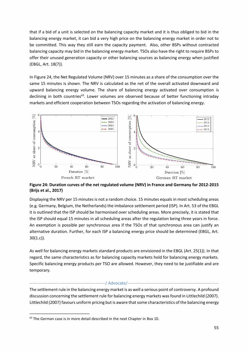
55
that if a bid of a unit is selected on the balancing capacity market and it is thus obliged to bid in the
balancing energy market, it can bid a very high price on the balancing energy market in order not to
be committed. This way they still earn the capacity payment. Also, other BSPs without contracted
balancing capacity may bid in the balancing energy market. TSOs also have the right to require BSPs to
offer their unused generation capacity or other balancing sources as balancing energy when justified
(EBGL, Art. 18(7)).
In Figure 24, the Net Regulated Volume (NRV) over 15 minutes as a share of the consumption over the
same 15 minutes is shown. The NRV is calculated as the net of the overall activated downward and
upward balancing energy volume. The share of balancing energy activated over consumption is
declining in both countries63. Lower volumes are observed because of better functioning intraday
markets and efficient cooperation between TSOs regarding the activation of balancing energy.
Figure 24: Duration curves of the net regulated volume (NRV) in France and Germany for 2012-2015 (Brijs et al., 2017)
Displaying the NRV per 15 minutes is not a random choice. 15 minutes equals in most scheduling areas
(e.g. Germany, Belgium, the Netherlands) the imbalance settlement period (ISP). In Art. 53 of the EBGL
it is outlined that the ISP should be harmonised over scheduling areas. More precisely, it is stated that
the ISP should equal 15 minutes in all scheduling areas after the regulation being three years in force.
An exemption is possible per synchronous area if the TSOs of that synchronous area can justify an
alternative duration. Further, for each ISP a balancing energy price should be determined (EBGL, Art.
30(1.c)).
As well for balancing energy markets standard products are envisioned in the EBGL (Art. 25(1)). In that
regard, the same characteristics as for balancing capacity markets hold for balancing energy markets.
Specific balancing energy products per TSO are allowed. However, they need to be justifiable and are
temporary.
------------------------------------------------------/ Advocate/-----------------------------------------------------------------
The settlement rule in the balancing energy market is as well a serious point of controversy. A profound
discussion concerning the settlement rule for balancing energy markets was found in Littlechild (2007).
Littlechild (2007) favours uniform pricing but is aware that some characteristics of the balancing energy
63 The German case is in more detail described in the next Chapter in Box 10.

56
market make it in some situations more difficult to apply this rule. In his paper64, he mentioned a
paragraph taken from the original proposals for NETA (Review of Electricity Trading Arrangements:
Proposals, Offer, July 1998, para 4.49.) wherein an argument in favour of pay-as-bid in the balancing
market is given: “The balancing market will be open for several hours, including real time operation.
During this period conditions on the system will be continuously changing. Trades may be accepted at
particular times at prices that are quite different from the average price of accepted trades over the
period as a whole. Consequently, there is no obvious definition for the marginal or market clearing price
throughout the period. To pay a uniform accepted price on all increments of generation and decrements
of demand, which would presumably have to be the highest price accepted from any one of them,
would not obviously be more efficient and could be expensive.” Littlechild (2007) adds that the weight
of this argument depends on the gap between the gate closure time and real operation65, which has
been decreasing since then, and the duration of the settlement period, which tends to decrease as
well.
Box 6: The settlement rule in balancing energy markets – specific technical difficulties and implementations in the Netherlands, Belgium and Spain
A problem, specific for balancing energy markets, arises when different products of different reserve types, for example, aFRR and mFRR, are used at the same instance. In the Netherlands, uniform pricing is applied, and the price is set by the highest bid of the two reserve types, even if this most expensive unit has only been activated for a very short fraction of the ISP (E-Brige Consulting, 2014). Another practical example illustrating why setting an adequate settlement rule in the balancing market was not obvious is the aFRR balancing market in Belgium (as it was in 2014). Because of technical reasons, the aFRR was employed on a pro-rata basis.66 A monthly tender for balancing capacity was organized to contract aFRR capacity. The selection of the balancing energy bids took place D-1 at 18:00, pre-contracted parties were obliged to offer their contracted bids, other parties could place voluntarily a bid. Elia selected up to 150 MW (upwards and downwards) according to their price starting with the lowest one. Then all bids that had been selected day-ahead were activated according to their participation factors for pro-rata activation and paid their bid price (E-Brige Consulting, 2014). Using the marginal pricing rule in this particular case seems contra intuitive. Today the selection of FRR bids is done using a merit order (Elia, 2017), making it more suitable for marginal pricing. In Spain, also the aFRR was deployed on a pro-rata basis and the pricing issue was solved by valuing the net energy usage (positive or negative) at the marginal price of RR that would have been
64 In Littlechild (2015) a similar argument is made, but phrased differently, it is stated that “in the balancing mechanism near real-time, the system operator does not see a nice stack of energy trades but rather chooses from a plethora of up and down actions each with different dynamic characteristics in the presence of noisy need. Some might be attractive enough to keep for several trading periods. Others will need to be reversed in favour of new opportunities or will come to an end because of self-dispatched movements. In such a context, the concept of marginal cost is a tenuous one. The most expensive 1 MWh bought or sold (even after flagging, tagging and offsetting) is not necessarily representative of the cost of a slight increase or reduction in capacity with respect to the half-hour as a whole.” 65 It could be argued that there are almost no significant material changes to the supply side dispatchable resources, except for contingencies, in e.g. the hour up to real-time. Renewables are obviously different and also the demand side may be a different matter. 66 On a discussion between pro rata activation and merit order selection of balancing energy, please consult E-Bridge and IAEW (2016). EBGL prescribes merit order selection of balancing energy bids.
57
necessary to use in the settlement period to replace the FRR energy delivered (Rodilla and Batlle, 2015).
--------------------------------------------------------------------------------------------------------------------------------------
In the EBGL (Art. 30(1.a)) it is clearly stated that the balancing energy market should be based on
marginal pricing. However, if all TSOs identify inefficiencies in the application of marginal pricing, they
may request an amendment and propose an alternative pricing method if proven more efficient (Art.
30(5)). It is added in Art. 30(1.b) that the methodology to determine prices for balancing energy shall
“define how the activation of balancing energy bids activated for purposes other than balancing affects
the balancing energy price, while also ensuring that at least balancing energy bids activated for internal
congestion management shall not set the marginal price of balancing energy.” This Article tackles a
concern of Littlechild (2007) who states that “marginal pricing may lead to erratic prices, especially
where the price order ‘stack’ can be distorted or ‘polluted’ by system actions taken by the System
Operator.” Another important point is made in Art. 30(1.c) stating that at least one price of balancing
energy for each ISP shall be established. ‘’At least one’’ could aim at multiple balancing energy prices
if both upward and downward energy is activated in the same ISP or could aim at different prices for
different types of reserves activated in the same direction.
Finally, cap and floor prices for balancing energy are optional. If applied they should be harmonised
and take into account the caps and floors applied in the day-ahead and intraday market (EBGL, Art.
30(2)).
Imbalance settlement mechanism
In this section, it is discussed how the imbalance price or charge67, the price an unbalanced BRP need
to pay (or receive), should be set. In real-time, the allocated volume (physical real-time energy
consumption/generation by a BRP) is not exactly the same as the contractual position for a given
imbalance settlement period. Two situations can occur:
• The BRP can have a positive imbalance (long), this implies that: o If the BRP is a net buyer, he consumes less electricity than its position. o If a BRP is a net seller, he produces more electricity than its position.
• The BRP can have a negative imbalance (short), this implies that: o If the BRP is a net buyer, he consumes more electricity than its position. o If a BRP is a net seller, he produces less electricity than its position
In the EBGL (Art. 55) it is specified that each TSO shall set up rules to calculate the imbalance price and
that an imbalance price shall be calculated for: each imbalance settlement period, imbalance price
areas and each imbalance direction. The financial flows between TSOs and BRPs are displayed in Table
2. Individual BRPs receive/pay an imbalance settlement depending on the direction of their imbalance.
By convention, if the imbalance is positive the BRP will receive the imbalance price multiplied by the
volume of its imbalance. If the imbalance is negative, the BRP will pay the imbalance price multiplied
67 Also called ‘’cash-out price’’ in the UK.
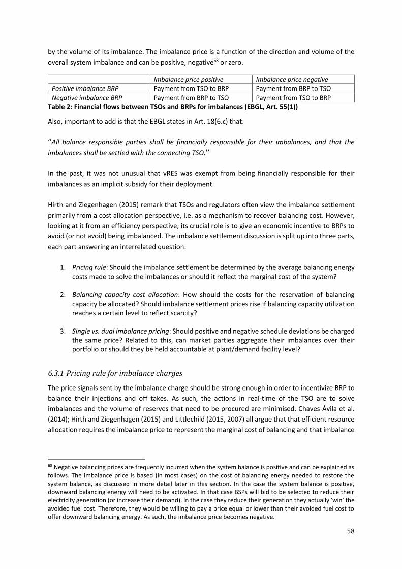
58
by the volume of its imbalance. The imbalance price is a function of the direction and volume of the
overall system imbalance and can be positive, negative68 or zero.
Imbalance price positive Imbalance price negative
Positive imbalance BRP Payment from TSO to BRP Payment from BRP to TSO
Negative imbalance BRP Payment from BRP to TSO Payment from TSO to BRP
Table 2: Financial flows between TSOs and BRPs for imbalances (EBGL, Art. 55(1))
Also, important to add is that the EBGL states in Art. 18(6.c) that:
‘’All balance responsible parties shall be financially responsible for their imbalances, and that the
imbalances shall be settled with the connecting TSO.’’
In the past, it was not unusual that vRES was exempt from being financially responsible for their
imbalances as an implicit subsidy for their deployment.
Hirth and Ziegenhagen (2015) remark that TSOs and regulators often view the imbalance settlement
primarily from a cost allocation perspective, i.e. as a mechanism to recover balancing cost. However,
looking at it from an efficiency perspective, its crucial role is to give an economic incentive to BRPs to
avoid (or not avoid) being imbalanced. The imbalance settlement discussion is split up into three parts,
each part answering an interrelated question:
1. Pricing rule: Should the imbalance settlement be determined by the average balancing energy costs made to solve the imbalances or should it reflect the marginal cost of the system?
2. Balancing capacity cost allocation: How should the costs for the reservation of balancing capacity be allocated? Should imbalance settlement prices rise if balancing capacity utilization reaches a certain level to reflect scarcity?
3. Single vs. dual imbalance pricing: Should positive and negative schedule deviations be charged the same price? Related to this, can market parties aggregate their imbalances over their portfolio or should they be held accountable at plant/demand facility level?
6.3.1 Pricing rule for imbalance charges
The price signals sent by the imbalance charge should be strong enough in order to incentivize BRP to
balance their injections and off takes. As such, the actions in real-time of the TSO are to solve
imbalances and the volume of reserves that need to be procured are minimised. Chaves-Ávila et al.
(2014); Hirth and Ziegenhagen (2015) and Littlechild (2015, 2007) all argue that that efficient resource
allocation requires the imbalance price to represent the marginal cost of balancing and that imbalance
68 Negative balancing prices are frequently incurred when the system balance is positive and can be explained as follows. The imbalance price is based (in most cases) on the cost of balancing energy needed to restore the system balance, as discussed in more detail later in this section. In the case the system balance is positive, downward balancing energy will need to be activated. In that case BSPs will bid to be selected to reduce their electricity generation (or increase their demand). In the case they reduce their generation they actually ‘win’ the avoided fuel cost. Therefore, they would be willing to pay a price equal or lower than their avoided fuel cost to offer downward balancing energy. As such, the imbalance price becomes negative.
59
settlements based on average costs may increase incentives for market parties to intentionally deviate
from their schedule.
------------------------------------------------------/ Advocate/-----------------------------------------------------------------
This discussion, whether the average cost for balancing energy or the marginal balancing energy cost
should set the imbalance price, cannot be decoupled from the settlement rule for balancing energy.
Two cases can be distinguished:
1.) Pay-as-bid for balancing energy: In this case, BSPs who are activated receive the price of their bid.
This means that the average balancing energy cost (average price paid to all BSPs) will be lower69 than
the cost of the marginal balancing action. A choice can be made whether the imbalance price should
equal the average balancing energy cost or the cost of the marginal action. In the former, a zero-sum
situation is created. In the latter, a surplus would result for the TSO.
2.) Marginal pricing of balancing energy: In this case, BSPs who are activated all receive the price of
the marginal bid. This means that the average balancing energy cost (price paid to all BSPs) equals the
cost of the marginal balancing action. Therefore, in this case the answer is trivial; it does not matter
whether the average or marginal cost of balancing energy sets the imbalance price as they are the
same. As mentioned previously, marginal pricing of balancing energy is also put forward in the EBGL.70
Box 7: The “Price Average Reference Volume (PAR)” approach in the UK (based on ACER/CEER (2016) Littlechild (2015, 2007) and Ofgem (2015))
In the UK, a hybrid methodology is in place; the so-called chunky marginal concept is introduced to come to a cost in between the average and marginal cost. The reasoning goes as follows. As it is not easy to determine the real marginal cost of balancing actions, due to the activation of balancing energy for other purposes, the mix of the activation of several balancing products with different time length, etc. some sort of “representative” figure for the cost of balancing actions needs to be found. As a solution, the imbalance price is set equal to the average cost of the most expensive X MWh of balancing purchases during a settlement period, defined as the Price Average Reference Volume (PAR)). As such, a sliding scale is obtained between on one end, applying the average cost, and on the other end, applying the marginal cost of balancing actions to set the imbalance price. The setting of PAR determines whether the imbalance price lends more towards the average or marginal cost. Historically the PAR was set to 500 MWh. It is proposed to gradually reduce the average cost of the most expensive 500 MWh balancing actions to the most expensive 50MWh (PAR50) in November 2015, before reducing it to 1MWh (PAR1) in the winter of 2018.
--------------------------------------------------------------------------------------------------------------------------------------
Further, in EBGL Art. 55 (4,5) it is specified that:
“4. The imbalance price for negative imbalance shall not be less than, alternatively:
69 Or equal in an extreme case. 70 However, if all TSOs identify inefficiencies in the application of marginal pricing, they may request an amendment and propose an alternative pricing method if proven more efficient (Art. 30(5)).

60
(a) the weighted average price for positive activated balancing energy from frequency restoration reserves and replacement reserves;
(b) in the event that no activation of balancing energy in either direction has occurred during the imbalance settlement period, the value of the avoided activation of balancing energy from frequency restoration reserves or replacement reserves. 5. The imbalance price for positive imbalance shall not be greater than, alternatively: (a) the weighted average price for negative activated balancing energy from frequency restoration reserves and replacement reserves; (b) in the event that no activation of balancing energy in either direction has occurred during the imbalance settlement period, the value of the avoided activation of balancing energy from frequency restoration reserves or replacement reserves. ”
6.3.2 Balancing capacity cost allocation
Before starting the discussion about how to allocate the cost of balancing capacity, it is important to
have an insight on how significant this cost is relative to the balancing energy cost. In Figure 25 the
overall balancing cost and its components over the national electricity consumption for the year 2015
are shown. Additionally, it is also shown what proportion of the balancing costs are covered by
imbalance charges.
Figure 25: Overall cost of balancing (energy71 plus capacity) and imbalance charges over the electricity consumption per country in 2015 (ACER/CEER, 2016)
Three observations can be made from Figure 25:
• The total balancing costs over national electricity consumption are very heterogeneous.
• For almost all countries the balancing capacity cost is significantly higher than the balancing energy cost.
• Total imbalance charges are in most countries similar to balancing energy cost, but far from enough to cover the total cost of balancing.
71 For the purpose of this calculation, the unit cost of activating balancing energy is defined as the difference between the balancing energy price of the relevant product and the DA market price.
61
In this section, we focus on observation 2 and 3, more precisely on how to allocate the balancing
capacity cost which is shown to be a strong driver of overall balancing costs. ACER/CEER (2016)
mention two important solutions to lower the cost of balancing capacity. Firstly, the integration of
balancing markets which would allow for the joint procurement and sharing of reserves72. And
secondly, the maximum participation of all technologies in the provision of balancing capacity,
including vRES, storage and DR. The EBGL is in place to foster the realisation of both complementary
solutions to lower the balancing capacity cost.
Traditionally, and still in place in most EU countries today, the balancing capacity procurement costs
are socialised. Network users pay these through network charges, or these costs are allocated to BRPs
in proportion to their consumed or produced energy volumes (ACER/CEER, 2016). It can be argued that
by socialising the cost of reserving balancing capacity not the right signals are being sent to market
parties.
------------------------------------------------------/ Advocate/-----------------------------------------------------------------
First, by socialising capacity costs, the large generators which actually motivate the scale of the
reserves might be insufficiently charged for the costs they cause to the system. Neuhoff et al. (2015a)
describe this problem as: ‘’this [the allocation the cost of balancing capacity procurement to those that
cause the need for these reservations] does not imply that the costs of paying for availability of reserves
should be allocated to the imbalance of the specific hour, e.g. by spreading the availability costs for the
hour across the parties that are in imbalance in this hour. Otherwise, imbalance prices may be very high
at times of low imbalance volumes (example Germany). Most availability costs for reserves are thus
born by demand and intermittent generation that creates frequent but small-scale deviations rather
than large generators that may cause large imbalances that motivated the scale of reserve provision,
but are only infrequent in imbalance.’’ Also Vandezande et al. (2010) state that the capacity costs for
reserves should not be socialized, but borne by those BRPs that cause the need for reservation.
At the same time, BSPs who could provide flexibility at moments of stress, which are exactly the
moments wherefore balancing capacity is procured, are not incentivised if prices are not high enough.
The same holds for BRPs not being sufficiently incentivised to be balanced at those particular
moments.
A solution, called Operating Reserve Demand Curves (ORDC), is brought forward in the literature (see
e.g. Hogan (2013) and Papavasiliou and Smeers (2017)) and already implemented in some parts of the
US (e.g. in Texas, see e.g. Levin and Botterud (2015)) and in the UK (ACER/CEER, 2016). Please note
that implementation in the UK differs from that in Texas (and details matter), but the philosophy
behind the approach is similar. The rationale behind ORDC is to introduce an incentive component
when balancing reserves are depleted to a certain level, and the probability of the loss of load becomes
non-negligible. This makes sense as by being imbalanced at moments of high system stress, there is
not only an energy cost related to solving the imbalance itself but also an increased probability of loss
of load. To put a price on this incentive component, the Value of Lost Load (VOLL) and the Loss of Load
Probability (LOLP) mapped on the volume of available reserves need to be estimated. Especially a
72 This is further elaborated upon in Section 7.2.2.

62
“correct” determination of the VOLL is a hard assignment and necessarily implies an administrative
intervention, making this procedure more difficult to implement.
By applying ORDC, imbalance prices could rise higher than the marginal cost of delivering balancing
energy. If only imbalance prices rise and not balancing energy prices (as in the UK implementation),
the balancing capacity procurement costs could be (partly) recuperated. With rising imbalance prices
BRPs are strongly incentivised to be balanced at moments of system stress. But, it could also be chosen
to not only let imbalance prices but also balancing energy prices rise at moments of system stress by
applying ORDC (as in the US implementation). In this case, not only BRPs will be motivated to be
balanced, but also BSPs will be stronger incentivised to be available in real-time at moments they are
needed the most73. In this case, a similar outcome could be achieved by not having balancing energy
price caps. However, as stated by Hogan (2013), it would be very difficult if not impossible to
distinguish scarcity prices from the exercise of market power. Closing the loop, both implementations,
with varying degrees, will lower the need for high volumes of balancing capacity to be procured,
leading to lower total balancing capacity costs to be recuperated.
Please note the difference between ORDC and a penalty added to the imbalance price, as also
described in Vandezande et al. (2010). First, a penalty is typically applied to the imbalance price in one
imbalance direction, not on both imbalance directions. Second, a penalty is in most cases triggered
when a certain threshold of balancing energy is activated in real-time. Activation of high volumes of
balancing energy does not necessarily imply a situation of system stress as there might be high volumes
of reserves available.
--------------------------------------------------------------------------------------------------------------------------------------
Related to the allocation of balancing capacity procurement costs, in Art. 44(3) of the EBGL it is stated
that:
‘’Each TSO may develop a proposal for an additional settlement mechanism separate from the imbalance settlement, to settle the procurement costs of balancing capacity (pursuant to Chapter 5 of this Title74), administrative costs and other costs related to balancing. The additional settlement mechanism shall apply to balance responsible parties. This should be preferably achieved with the introduction of a shortage pricing function. If TSOs choose another mechanism, they should justify this in the proposal. Such a proposal shall be subject to approval by the relevant regulatory authority. ‘’
6.3.3 Single vs. dual imbalance pricing
Imagine an imbalance settlement period wherein the system is short of power. In that case, the
imbalance price is expected to be positive as it is related to the activated upward balancing power.
Now, in that case, should a BRP having a negative imbalance (short), thus contributing to the system
imbalance, be charged the same imbalance price a positively imbalanced BRP (long), helping the
system, receives?
73 Or even stronger, this approach could (partly) solve the missing money problem as giving an additional incentive for flexible generation to be installed. 74 EBGL Article 56: Procurement within a scheduling area 1. Each TSO of a scheduling area using balancing capacity bids shall establish rules for the settlement of at least frequency restoration reserves and replacement reserves pursuant to the requirements set out in Article 32. 2. Each TSO of a scheduling area using balancing capacity bids shall settle at least all procured frequency restoration reserves and replacement reserves pursuant to the requirements set out in Article 32.
63
Single imbalance pricing implies a ‘’Yes’’ to this answer, while with dual imbalance pricing a different
imbalance price would be charged to the short BRP than the long BRP would receive. In EU countries
today both single, dual and hybrid pricing is in place (ENTSO-E, 2017g). Single pricing is often favoured
over a dual pricing in the academic literature (Chaves-Ávila and Fernandes, 2015; Hiroux and Saguan,
2010; Littlechild, 2007; Neuhoff et al., 2015a; Newbery, 2006). Under dual pricing, the reverse price
(individual imbalances in the opposite direction of the system imbalance) is often linked or capped by
a reference or day-ahead market price, while the imbalance in the direction of the system imbalance
is linked to the cost of balancing energy.
Art. 32(2) of the EBGL is relevant for this matter. Single pricing should be applied. However, a TSO may
propose to the NRA to apply dual pricing under certain conditions and with the necessary justification.
More precisely:
‘’By one year after entry into force of this Regulation, all TSOs shall develop a proposal to further specify
and harmonize at least:
….
(c) the use of single imbalance pricing for all imbalances pursuant to Article 55, which defines a single
price for positive imbalances and negative imbalances for each imbalance price area within an
imbalance settlement period; and
(d) the definition of conditions and methodology for applying dual imbalance pricing for all imbalances
pursuant to Article 55, which defines one price for positive imbalances and one price for negative
imbalances for each imbalance price area within an imbalance settlement period, encompassing:
(i) conditions on when a TSO may propose to its relevant regulatory authority in accordance
with Article 37 of Directive 2009/72/EC the application of dual pricing and which justification
must be provided;
(ii) the methodology for applying dual pricing.’’
------------------------------------------------------/ Advocate/-----------------------------------------------------------------
Many arguments in favour of single pricing are found in the academic literature. An important
argument is the fact that dual imbalance pricing discriminates against smaller generation units where
companies can aggregate imbalances within a portfolio (Neuhoff et al., 2015a). This is especially the
case if there is no liquid intraday market to trade imbalances (Chaves-Ávila et al., 2014). Also, a single
imbalance price would constitute a suitable liquid reference price. Further, the dual price imbalance
design is reputed to be less cost-reflective than the single price design (Newbery, 2006). Littlechild
(2007) puts it as: “[with dual pricing] the reverse price (individual imbalances in the opposite direction
of the system imbalance in a dual price system) has been ‘deliberately delinked’ from the System
Operator’s costs. It is difficult to see how this is consistent with the stated philosophy of setting
imbalance prices to reflect the System Operator’s costs. And by linking the imbalance prices with the
short-term market prices the risk of distorting the traded market by introducing incentives to influence
that market price in order to influence imbalance price is run.”
64
Another important argument brought up by Littlechild (2007) in favour of single pricing is that under
that mechanism both short and long BRPs participants can contribute to balancing the system, but the
dual pricing encourages only one set of market participants to do so.75 This argument relates to Hirth
and Ziegenhagen (2015) who see two types of balancing: active and passive balancing. When TSOs
deploy balancing energy, they actively balance the system. However, when the imbalance price
provides the right incentive to BRPs, these can “passively” balance the system by purposely deviating
from the schedule. This is also called self-balancing. Three preconditions are needed for effective
passive balancing: single pricing, a timely publication of the imbalance price76, and the legal ability for
BRPs to respond to the price signal (which has not been the case for Germany in the past).
There are also arguments formulated in favour of dual pricing over single pricing. Brijs et al. (2017) and
Vandezande (2011) note that speculation of BRPs on the direction of the system imbalance would be
avoided with dual pricing. In that same line, if BRPs do not passively balance themselves, it would be
easier for the TSO to estimate real-time system imbalances and anticipate power flows. This is
especially of importance when internal grid congestion is a frequent issue. An interesting point is made
by Chaves-Ávila et al. (2014). In their paper, they mention the fact that a single pricing scheme for a
whole country can lead to misleading imbalance prices in the context of internal congestion splitting
the scheduling zone into two areas. In that case, market parties can be incentivized to worsen their
local imbalance if the imbalance direction is opposite in the different areas. A similar remark is made
by Brunekreeft (2015). He states that if the imbalance in one settlement period changes from positive
to negative (or the other way around), for one of these imbalances, the imbalance price would be
wrong and would set the wrong incentives. In fact, everything would go the other way around, and the
system would destabilize. Chaves-Ávila et al. (2014) argue that a nodal or zonal pricing would solve the
issue, but that this solution is hard to implement today because of several reasons. A temporary
solution would be to use a hybrid pricing rule, more precisely using single pricing when there is a
unique direction of regulation and dual pricing when both upward and downward reserves are
activated. Chaves-Ávila et al. (2014) conclude that such a scheme can result in a lower efficiency of
cost allocation, but that it prevents adverse destabilising price signals. This is also the regulation put in
place in the Dutch system today (Brunekreeft, 2015).
--------------------------------------------------------------------------------------------------------------------------------------
The last point, directly related to single or dual pricing is whether market parties should be responsible
for their imbalances at plant/demand facility level or whether aggregation of their imbalances over
their portfolio is allowed, defined as balancing groups by Neuhoff et al. (2016c). Today in Europe this
rule is not harmonised (ENTSO-E, 2017g). Balance responsibility on an individual level is compatible
with the single pricing, as mentioned before; the financial outcome when imbalances are accounted
for individually or on an aggregated scale will not differ. On the contrary, if dual pricing is implemented
aggregation will make a difference in the total cost, favouring large portfolios. Additionally, Neuhoff et
al. (2016c) argue that balancing groups have a cost for the system as it lowers the liquidity in the
75 Littlechild (2007) states: ‘’the significant gap between system buy and sell price seems likely to have distorted
decisions on how far each participant decides to balance its own position rather than use the facilities of the System Operator. Not surprisingly, many market participants seem to have taken the view that being short is to be avoided at almost all costs. This is unlikely to be efficient.’’ 76 EBGL (Art. 12(3.a)), each TSO shall publish: “Information on the current system imbalance of its scheduling area, as soon as possible but no later than 30 minutes after real-time.”
65
balancing market by encouraging balancing within groups and could have the effect that the TSO over-
contracts balancing capacity as it does not have a good oversight of balancing resources available in
the system. The authors argue that the design of the imbalance price can only partially compensate
for this effect and that the problem aggravates if transmission capacity within a scheduling zone is
scarce.
In Art. 54(3) of the EBGL it is left over to the individual TSOs to decide whether aggregation of
imbalances over a portfolio is allowed. More precisely, it is stated that ‘’each TSO shall calculate the
final position of a balance responsible party using one of the following approaches:
(a) balance responsible party has one single final position equal to the sum of its external commercial
trade schedules and internal commercial trade schedules;
(b) balance responsible party has two final positions: the first is equal to the sum of its external
commercial trade schedules and internal commercial trade schedules from generation, and the second
is equal to the sum of its external commercial trade schedules and internal commercial trade schedules
from consumption;’’
The activation of balancing energy: two approaches
Two approaches to the activation of balancing energy are identified in the EU, reactive balancing and
proactive balancing (Elia and TenneT, 2014; Haberg and Doorman, 2016; Pentalateral Energy Forum,
2016). The key difference between the two approaches is that with reactive balancing the TSO
activates balancing energy to counteract imbalances in real-time, while with proactive balancing the
TSO activates balancing energy before real-time77 based on forecasts of imbalances. The activation
strategy of balancing energy cannot be decoupled from the reliance of a TSO on BRPs to self-balance
and thus the imbalance settlement mechanism. More responsibility is shifted to BRPs to be balanced
with a reactive activation strategy, BRPs can even be encouraged to (passively) restore the system
balance. Therefore, shorter imbalance settlement periods and single imbalance pricing fit well with
this approach. Oppositely, the proactive approach relies more strongly on active balancing by the TSO
and generally give weaker incentives to the BRPS.
An overview of a selection of EU countries and their approach to the activation of balancing energy is
shown in Figure 26. Additionally, in the same Figure, the relationship between BRP incentives and the
activation strategy is displayed. It can be seen that there are also countries (e.g. Denmark) applying an
approach in between reactive and proactive balancing.
77 At least one hour before real-time is mentioned by Pentalateral Energy Forum (2016).
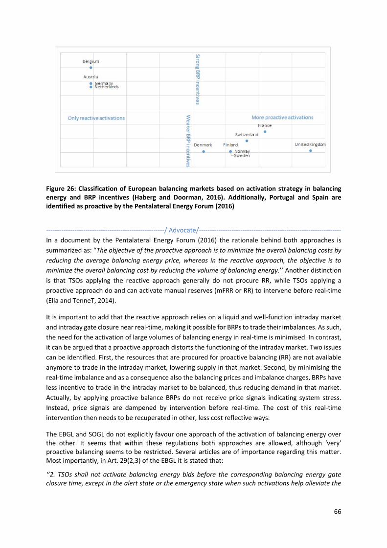
66
Figure 26: Classification of European balancing markets based on activation strategy in balancing energy and BRP incentives (Haberg and Doorman, 2016). Additionally, Portugal and Spain are identified as proactive by the Pentalateral Energy Forum (2016)
------------------------------------------------------/ Advocate/-----------------------------------------------------------------
In a document by the Pentalateral Energy Forum (2016) the rationale behind both approaches is
summarized as: “The objective of the proactive approach is to minimize the overall balancing costs by
reducing the average balancing energy price, whereas in the reactive approach, the objective is to
minimize the overall balancing cost by reducing the volume of balancing energy.’’ Another distinction
is that TSOs applying the reactive approach generally do not procure RR, while TSOs applying a
proactive approach do and can activate manual reserves (mFRR or RR) to intervene before real-time
(Elia and TenneT, 2014).
It is important to add that the reactive approach relies on a liquid and well-function intraday market
and intraday gate closure near real-time, making it possible for BRPs to trade their imbalances. As such,
the need for the activation of large volumes of balancing energy in real-time is minimised. In contrast,
it can be argued that a proactive approach distorts the functioning of the intraday market. Two issues
can be identified. First, the resources that are procured for proactive balancing (RR) are not available
anymore to trade in the intraday market, lowering supply in that market. Second, by minimising the
real-time imbalance and as a consequence also the balancing prices and imbalance charges, BRPs have
less incentive to trade in the intraday market to be balanced, thus reducing demand in that market.
Actually, by applying proactive balance BRPs do not receive price signals indicating system stress.
Instead, price signals are dampened by intervention before real-time. The cost of this real-time
intervention then needs to be recuperated in other, less cost reflective ways.
The EBGL and SOGL do not explicitly favour one approach of the activation of balancing energy over the other. It seems that within these regulations both approaches are allowed, although ‘very’ proactive balancing seems to be restricted. Several articles are of importance regarding this matter. Most importantly, in Art. 29(2,3) of the EBGL it is stated that:
‘’2. TSOs shall not activate balancing energy bids before the corresponding balancing energy gate closure time, except in the alert state or the emergency state when such activations help alleviate the
67
severity of these system states and except when the bids serve purposes other than balancing pursuant to paragraph 3.
3. By one year after the entry into force of this Regulation, all TSOs shall develop a proposal for a methodology for classifying the activation purposes of balancing energy bids. This methodology shall: (a) describe all possible purposes for the activation of balancing energy bids;
(b) define classification criteria for each possible activation purpose. ‘’ Looking back at Art. 24(1,2) of the EBGL, regarding the balancing energy GCT, it is stated that:
“1. As part of the proposals pursuant to Articles 19, 20 and 21, all TSOs shall harmonise the balancing energy gate closure time for standard products at the Union level, at least for each of the following processes:
(a) replacement reserves;
(b) frequency restoration reserves with manual activation;
(c) frequency restoration reserves with automatic activation.
2. Balancing energy gate closure times shall:
(a) be as close as possible to real time;
(b) not be before the intraday cross-zonal gate closure time;
(c) ensure sufficient time for the necessary balancing processes. ‘’
Further, in the CACM (Art. 59(3)), concerning the intraday cross-zonal GCT, is found:
“One intraday cross-zonal gate closure time shall be established for each market time unit for a given bidding zone border. It shall be at most one hour before the start of the relevant market time unit and shall take into account the relevant balancing processes in relation to operational security.”
These articles do imply that the balancing GCT will be at most one hour before real-time and would
mean that proactively activating balancing energy (if this activation is considered as being for balancing
purposes) long (a couple of hours) before real-time will not be allowed. However, on the other hand,
procurement of RR and having in place a Reserve Replacement Process (RRP), compatible with the
proactive balancing approach, is a right described in EBGL (Art. 19) and SOGL (Art. 140(2)). In Art.
144(1) of SOGL it is stated that:
‘’The control target of the RRP shall be to fulfil at least one of the following goals by activation of RR:
(a) progressively restore the activated FRR;
(b) support FRR activation;
(c) for the GB and IE/NI synchronous areas, to progressively restore the activated FCR and FRR.’’
Box 8: Self-dispatch versus central dispatch models
Several articles in the EBGL and the SOGL mention that (slightly) different provisions hold for self-dispatch or central dispatch systems, the two dispatch models applied in the EU. Self-dispatch models can be reactive or proactive in their activation of balancing energy. If a similar label should be put on central dispatch models, they can be categorised as extremely proactive in their balancing approach.
68
The self-dispatch model is the most common and defined ‘’as a scheduling and dispatching model where the generation schedules and consumption schedules as well as dispatching of power generating facilities and demand facilities are determined by the scheduling agents of those facilities’’ (EBGL, Art. 2(17)). On the contrary, with a central dispatch model ‘’the generation schedules and consumption schedules as well as dispatching of power generating facilities and demand facilities, in reference to dispatchable facilities, are determined by a TSO within the integrated scheduling process’’ ((EBGL, Art. 2(17)). With an integrated scheduling process is meant that balancing, reserve procurement and congestion management are done concurrently (Marneris and Biskas, 2015). In short, under the self-dispatch model different markets are organised for different purposes (balancing energy, balancing capacity and congestion management) and market parties with their economic incentives are more important, while under central dispatch an integrated process is executed with a much greater role for the TSO. Currently, the central dispatch model is in place in e.g. Greece, Hungary, Italy and Poland (Marneris and Biskas, 2015). Ireland is in a transition from a central dispatch to a self-dispatch model. The self-dispatch model is more in line with the European Target model (see also ACER (2015b) and Gorecki (2013)) and is seen as ‘’default’’ in the EBGL as can be deducted from Art. 14(2): ‘’Each TSO shall apply a self-dispatching model for determining generation schedules and consumption schedules. TSOs that apply a central dispatching model at the time of the entry into force of this Regulation shall notify to the relevant regulatory authority in accordance with Article 37 of Directive 2009/72/EC in order to continue to apply a central dispatching model for determining generation schedules and consumption schedules. The relevant regulatory authority shall verify whether the tasks and responsibilities of the TSO are consistent with the definition in Article 2(18).’’ Therefore, the working of the balancing mechanism described in this Chapter and the next Chapter refers to the self-dispatch model. Otherwise, it will be explicitly stated.
--------------------------------------------------------------------------------------------------------------------------------------
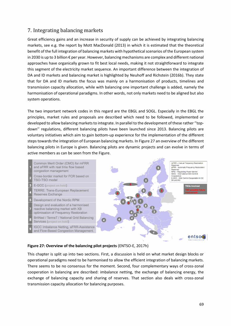
69
7. Integrating balancing markets
Great efficiency gains and an increase in security of supply can be achieved by integrating balancing
markets, see e.g. the report by Mott MacDonald (2013) in which it is estimated that the theoretical
benefit of the full integration of balancing markets with hypothetical scenarios of the European system
in 2030 is up to 3 billion € per year. However, balancing mechanisms are complex and different national
approaches have organically grown to fit best local needs, making it not straightforward to integrate
this segment of the electricity market sequence. An important difference between the integration of
DA and ID markets and balancing market is highlighted by Neuhoff and Richstein (2016b). They state
that for DA and ID markets the focus was mainly on a harmonisation of products, timelines and
transmission capacity allocation, while with balancing one important challenge is added, namely the
harmonisation of operational paradigms. In other words, not only markets need to be aligned but also
system operations.
The two important network codes in this regard are the EBGL and SOGL. Especially in the EBGL the
principles, market rules and proposals are described which need to be followed, implemented or
developed to allow balancing markets to integrate. In parallel to the development of these rather ‘’top-
down’’ regulations, different balancing pilots have been launched since 2013. Balancing pilots are
voluntary initiatives which aim to gain bottom-up experience for the implementation of the different
steps towards the integration of European balancing markets. In Figure 27 an overview of the different
balancing pilots in Europe is given. Balancing pilots are dynamic projects and can evolve in terms of
active members as can be seen from the Figure.
Figure 27: Overview of the balancing pilot projects (ENTSO-E, 2017h)
This chapter is split up into two sections. First, a discussion is held on what market design blocks or
operational paradigms need to be harmonised to allow the efficient integration of balancing markets.
There seems to be no consensus for the moment. Second, four complementary ways of cross-zonal
cooperation in balancing are described: imbalance netting, the exchange of balancing energy, the
exchange of balancing capacity and sharing of reserves. That section also deals with cross-zonal
transmission capacity allocation for balancing purposes.
70
How far should harmonisation go to allow for integration?
In earlier drafts of the EBGL, e.g. the version 3.0 published on the 30th of August 201478, a concept
called Coordinated Balancing Areas (CoBAs) was mentioned. In that version of the EBGL, CoBAs are
defined as “a cooperation with respect to the Exchange of Balancing Services, Sharing of Reserves or
operating the Imbalance Netting Process between two or more TSOs.”
The main idea behind CoBAs was a phased approach toward the full integration of balancing markets.
First, regional initiatives (as with the balancing pilots), allowing for more flexibility in design, would
emerge which would then slowly be merged. ACER (2015c) also confirmed that a regional
implementation is an unavoidable interim step to single EU-wide integration. However, CoBAs were
removed in the final version of the EBGL (approved by the MSs on 16 March 2017), and the focus was
laid more strongly on the (single) European Target Model. However, the line of thought behind CoBAs
is not fully discarded, and regional initiatives are still deemed the way forward as stated by TenneT et
al. (2016).
------------------------------------------------------/ Advocate/-----------------------------------------------------------------
Box 9: Two regional balancing initiatives – TERRE and EXPLORE
Two regional balancing initiatives often referred to are TERRE and EXPLORE. It is interesting to look deeper into these two initiatives as they have different objectives and indicate the emergence (or rather a continuation?) of two diverging philosophies to balancing. TERRE stands for ‘’Trans European Replacement Reserves Exchange’’ and has 8 active partners: two TSOs in Great Britain, the TSOs from France, Spain, Portugal, Italy, Switzerland and Greece. The TSOs from Ireland and North Ireland are observers. ENTSO-E (2017g) described the objective of TERRE as: “setting up and operating a multi-TSO platform capable of gathering all the offers for Replacement Reserves (RR) and to optimise the allocation of RR across the systems of the different TSOs involved. It is moving towards cross-national exchange of RR.’’ It is no coincidence that all TSOs involved in the project apply a rather proactive approach to the activation of balancing energy. Neuhoff and Richstein (2016b) add that the TERRE countries provide room for the continuation of national procedures as the operational paradigms between these countries, although all rather proactive, still significantly differs. EXPLORE stands for ‘’European X-border Project for LOng term Real-time balancing Electricity market design” and is an initiative of the TSOs of four countries: Austria, Belgium, Germany and the Netherlands. The objective of the EXPLORE study is to investigate how to exchange most optimally Frequency Restoration Reserves (FRR) while taking into account interactions with other balancing processes and the spot market. All countries participating in this project apply a reactive approach to the activation of balancing energy and, in contrast to the TERRE countries, show more commonalities in their approach to the balancing mechanism as also confirmed by Neuhoff and Richstein (2016).
In a document by the Pentalateral Energy Forum (2016), it is remarked that ACER and ENTSO-E hold
different views on the degree of harmonisation needed across regional initiatives. ACER reasons that
a sufficient degree of harmonisation is needed in order to avoid getting stuck with incompatible
78https://www.entsoe.eu/Documents/Network%20codes%20documents/NC%20EB/140806_NCEB_Resubmission_to_ACER_v.03.PDF
71
regions, while it is stated in that document that ENTSO-E is of the opinion that regional balancing
initiatives can start without complete harmonisation.
Standardised balancing products and a harmonised balancing energy gate closure time (GCT) are the
two dimensions that both parties agree upon that are absolutely necessary for integration. The EBGL
outlines that standard balancing products need to be defined in Art. 25. However, if requested by a
TSO and justified, temporarily specific balancing products might be in place in parallel to standard
products (Art. 26(1)). The EBGL also states that these standardised balancing energy products for
mFRR, aFRR and RR need to be exchanged on European trading platforms (EBGL, Art. 19, 20 and 21).
Regarding the balancing energy GCT, in Art. 24(1) of the EBGL it is firmly stated the GCT for
standardised products should be harmonised for at least mFRR, aFRR and RR processes.
Other two no-regret options needed for the integration of balancing markets as stated by Neuhoff and
Richstein (2016), and also agreed upon by ACER (2015c), are the harmonisation of the imbalance
settlement period (ISP) and the agreement on the settlement of balancing energy markets. Regarding
the former and as already mentioned in the previous chapter, the EBGL states clearly that the ISP
should be 15 minutes in all control areas (EBGL, Art.53(1)). The only exemption to this rule could take
place if all TSOs of a synchronous area propose and justify an alternative ISP for their synchronous area
(EBGL, Art. 53(2-3)). Also, the latter was already discussed in the previous chapter and is determined
in the EBGL. In Art. 30(1.a) of the EBGL it is stated that marginal pricing should be applied. TSOs might
propose an amendment or alternative to this rule if they can identify inefficiencies in the application
of this methodology (EBGL, Art. 30(5)).
Next to the three already mentioned dimensions of balancing markets, it is argued by ACER (2015c)
that there is a need to go further to avoid diverging regional designs. Additional dimensions identified
are principles for (activation) algorithms and TSO-TSO settlement rules79. In the document by the
Pentalateral Energy Forum (2016) the need to harmonise the activation purposes of balancing energy
is added to the view of ACER.
--------------------------------------------------------------------------------------------------------------------------------------
Inter-TSO cooperation in balancing
Four complementary ways of coordinated balancing are identified in the EBGL and SOGL. In the
following, they are described two per two. First, imbalance netting and the exchange of balancing
energy are bundled as they more directly affect the balancing energy market. After, the exchange of
balancing capacity and sharing of reserves are jointly discussed. These ways of coordinated balancing
have a more direct impact on the balancing capacity market. The exchange of balancing capacity and
sharing of reserves add a layer of difficulty as cross-zonal transmission capacity must be reserved or
anticipated for to serve these purposes. In contrast, for imbalance netting and the exchange of
balancing energy, cross-zonal capacity must be available as these processes take place in real-time.
79 TSO-TSO settlement rules are discussed in the next section of the chapter.
72
Box 10: ‘The German Paradox’ – more renewables but less and cheaper reserves?
Generally, the idea is that with an increased share of vRES in the system the reserve requirements would increase as well, this seems to be intuitive. But this is not necessarily the case. While in Germany the vRES capacity has tripled since 2008, reserve requirements have been reduced by 15 %, and costs by 50% by 2014. (Hirth and Ziegenhagen, 2015). This indicates that other factors can be quantitatively more important than vRES in determining the reserve requirement. Ocker and Ehrhart (2017) investigate this paradox in their paper and attribute the reduction in reserve requirement, next to better forecasting techniques of vRES generation, to two factors: International and national cooperation: from 2009 to 2010 the four German TSOs introduced a common balancing market80, as such counteracting activations of balancing energy in different balancing areas could be avoided and fewer reserves needed to be procured, leading to significant savings (see also Haucap et al. (2014)). Additionally, the International Grid Control Cooperation (IGCC)81 was founded by which significant amounts of balancing energy was saved. Adaptations in the German energy market design: a strong increase in intraday trading was witnessed from 2006-2014. Intraday trade leads to a reduced need for balancing. Additionally, it is argued that the introduction of the intraday action with 15-minutes products in December 2014 helped to allow the expected energy production of vRES and other generation technologies to be closer to the actual energy production due to its finer time granularity.
7.2.1 Less and cheaper balancing energy: imbalance netting and the exchange of balancing
energy
Imbalance netting is defined in Article 3(128) of the SOGL as “a process agreed between TSOs that
allows avoiding the simultaneous activation of FRR in opposite directions, taking into account the
respective FRCEs as well as the activated FRR and by correcting the input of the involved FRPs
accordingly.” Simpler, if for example, two neighbouring LFC Areas have at a point in time an opposite
system imbalance, the TSOs can agree to exchange the imbalance, and as such, the activation of
counteracting balancing energy (FRR in this case) in both LFC Areas can be avoided. This process leads
to an overall reduction in the total volume of activated balancing energy and thus a cost reduction.
ACER/CEER (2016) report that imbalance netting continued to be the most successfully applied tool to
exchange balancing services in 2015, e.g. in the Netherlands imbalance netting avoided almost 50 %
of the balancing needs for that year.
Art. 22(1) of the EBGL outlines that a European Platform for imbalance netting shall be developed. In
Art. 22(5) it is further stated that: ‘’by one year after the approval of the proposal for the
implementation framework for a European platform for the imbalance netting process, all TSOs
performing the automatic frequency restoration process pursuant to Part IV of Commission Regulation
(EU) 2017/000 [SO] shall implement and make operational the European platform for the imbalance
netting process. They shall use the European platform to perform the imbalance netting process, at
least for the Continental Europe synchronous area.’’ ENTSO-E (2017h) describes that TSOs have gained
80 The project, called the German Grid Control Cooperation (GCC), consists out of 4 modules: 1.) Prevent counteracting reserve activation 2.) Common dimensioning of reserves 3.) Common procurement of FRR 4.) Cost-optimised activation of reserves. For more info, please consult Regelleistung.net (2017). 81 The IGCC is further developed in the next Section.
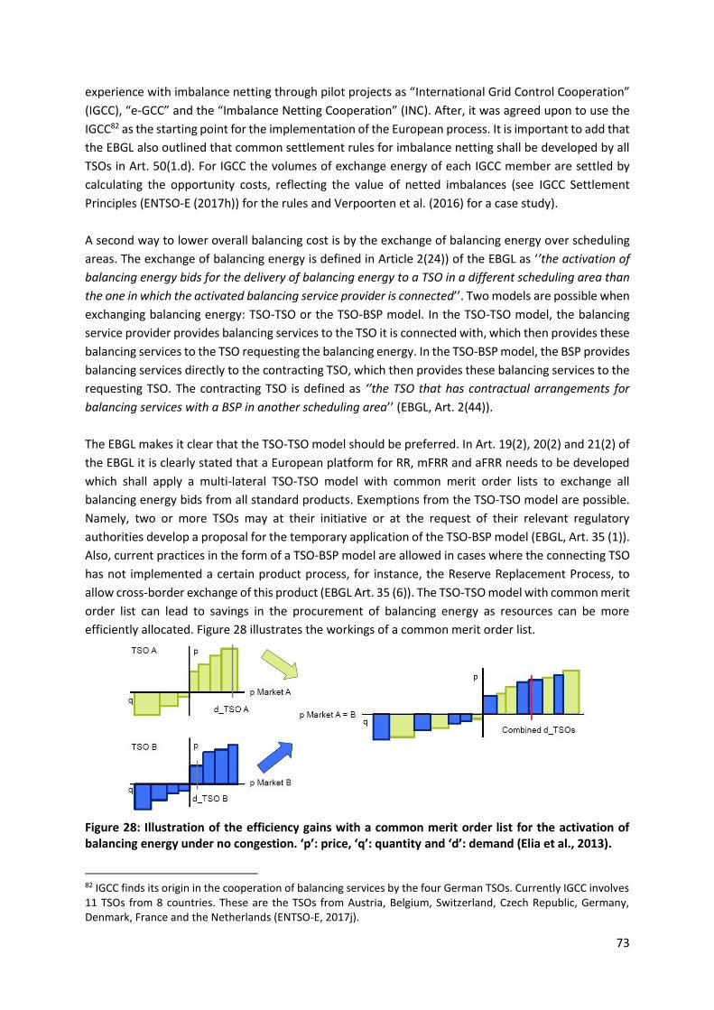
73
experience with imbalance netting through pilot projects as “International Grid Control Cooperation”
(IGCC), “e-GCC” and the “Imbalance Netting Cooperation” (INC). After, it was agreed upon to use the
IGCC82 as the starting point for the implementation of the European process. It is important to add that
the EBGL also outlined that common settlement rules for imbalance netting shall be developed by all
TSOs in Art. 50(1.d). For IGCC the volumes of exchange energy of each IGCC member are settled by
calculating the opportunity costs, reflecting the value of netted imbalances (see IGCC Settlement
Principles (ENTSO-E (2017h)) for the rules and Verpoorten et al. (2016) for a case study).
A second way to lower overall balancing cost is by the exchange of balancing energy over scheduling
areas. The exchange of balancing energy is defined in Article 2(24)) of the EBGL as ‘’the activation of
balancing energy bids for the delivery of balancing energy to a TSO in a different scheduling area than
the one in which the activated balancing service provider is connected’’. Two models are possible when
exchanging balancing energy: TSO-TSO or the TSO-BSP model. In the TSO-TSO model, the balancing
service provider provides balancing services to the TSO it is connected with, which then provides these
balancing services to the TSO requesting the balancing energy. In the TSO-BSP model, the BSP provides
balancing services directly to the contracting TSO, which then provides these balancing services to the
requesting TSO. The contracting TSO is defined as ‘’the TSO that has contractual arrangements for
balancing services with a BSP in another scheduling area’’ (EBGL, Art. 2(44)).
The EBGL makes it clear that the TSO-TSO model should be preferred. In Art. 19(2), 20(2) and 21(2) of
the EBGL it is clearly stated that a European platform for RR, mFRR and aFRR needs to be developed
which shall apply a multi-lateral TSO-TSO model with common merit order lists to exchange all
balancing energy bids from all standard products. Exemptions from the TSO-TSO model are possible.
Namely, two or more TSOs may at their initiative or at the request of their relevant regulatory
authorities develop a proposal for the temporary application of the TSO-BSP model (EBGL, Art. 35 (1)).
Also, current practices in the form of a TSO-BSP model are allowed in cases where the connecting TSO
has not implemented a certain product process, for instance, the Reserve Replacement Process, to
allow cross-border exchange of this product (EBGL Art. 35 (6)). The TSO-TSO model with common merit
order list can lead to savings in the procurement of balancing energy as resources can be more
efficiently allocated. Figure 28 illustrates the workings of a common merit order list.
Figure 28: Illustration of the efficiency gains with a common merit order list for the activation of balancing energy under no congestion. ‘p’: price, ‘q’: quantity and ‘d’: demand (Elia et al., 2013).
82 IGCC finds its origin in the cooperation of balancing services by the four German TSOs. Currently IGCC involves 11 TSOs from 8 countries. These are the TSOs from Austria, Belgium, Switzerland, Czech Republic, Germany, Denmark, France and the Netherlands (ENTSO-E, 2017j).
74
Also in the case of the exchange of balancing energy, the EBGL outlined that common settlement rules
shall be developed by all TSOs in Art. 50(1.a-c). Further, two remarks about the exchange of balancing
energy need to be added. First, the total balancing volume a TSO may request for activation from the
common merit order list is limited by its own contribution of balancing energy bids to the list (for more
details, see EBGL Art. 29(12)). Exemptions from this rule can be proposed by TSOs (EBGL, Art. 29(13)).
Second, a TSO can declare a balancing energy bid submitted to the activation function of the common
merit order list unavailable for the activation by other TSOs only in case of internal congestion or due
to operational constraints (EBGL, Art. 29(14)).
In order to conduct imbalance netting or the exchange of balancing energy, available transmission
capacity between scheduling areas or LFC Areas is a prerequisite.83 Related to this fact, in Art. 36(1) it
is demanded that all TSOs shall use the available cross-zonal capacity after the cross-zonal intraday
gate closure for the exchange of balancing energy or for operating the imbalance netting process.
Concretely, two situations can exist, assuming there is spare capacity in both directions between two
LFC Areas:
• The imbalances in both areas are opposite: First, imbalance netting will take place. Then, if the imbalance in one of the areas persists and the transmission line is not congested, the exchange of balancing energy can take place.
• The imbalances in both areas are in the same direction: No imbalance netting will take place. The exchange of balancing energy can take place.
A methodology per capacity calculation region will be developed to calculate the available cross-zonal
capacity within the balancing time frame (EBGL, Art 37(3)). In the EBGL it is not mentioned whether
cross-zonal capacity can be reserved specifically for imbalance netting or the exchange of balancing
energy84.
7.2.2 More efficient reserve procurement and sizing: exchange of reserves and reserves
sharing
Next to imbalance netting and the exchange of balancing energy, also the exchange of reserves and
reserve sharing are outlined in the EBGL as important to lower overall balancing procurement costs.
The exchange of balancing capacity is defined in Art. 2(25) of the EBGL as “the provision of balancing
capacity to a TSO in a different scheduling area than the one in which the procured BSP is connected.”
An example is a project for cross-border exchange of FCR capacity which started in late 2015 and
involved the German, Austrian, Dutch and Swiss TSOs. ACER/CEER (2016) reports that the exchange of
balancing capacity allowed a reduction of approximately 14% in the overall balancing capacity
procurement costs for FCR in 2015 when comparing with 2014 for these four countries recorded.
83 An exemption to this statement holds for the exchange and operation of FCR (EBGL, Art. 38(4)). FCR can be exchanged using the reliability margin, calculated as described by CACM, Art. 22. This exemption does not hold if the interconnector is a DC line. 84 However, as discussed in the next subsection, cross-zonal transmission capacity can be reserved for the exchange of balancing capacity or through the sharing of reserves. And thus, indirectly also for balancing energy exchange.
75
The same two models for the exchange of balancing capacity are possible as with the exchange of
balancing energy: TSO-TSO and the TSO-BSP model. Also, in this case, the EBGL states that the
exchange shall always be performed based on a TSO-TSO model unless the same exemptions as with
the exchange of balancing energy hold (EBGL, Art. 33(2)). As all TSOs engaged in exchanging balancing
capacity submit all balancing capacity bids from standard products to a common capacity procurement
optimisation function (EBGL, Art. 33(3)), a more efficient allocation of resources will result. Overall
balancing capacity reservation costs can be lowered, and BSPs can benefit from access to an enlarged
market without new pre-qualification procedures or contracts.
------------------------------------------------------/ Advocate/-----------------------------------------------------------------
However, as remarked by Doorman and Van Der Veen (2013), it might be more difficult to convince
TSOs to exchange balancing capacity than to exchange balancing energy. Namely, a TSO with low-cost
balancing resources may see an increase in its balancing procurement cost when sharing these
resources with areas with higher cost resources. In the case of balancing energy, these possibly
increased cost for that TSO will be passed on to BRPs causing the imbalances. In most cases, this will
be a zero sum for the TSO as discussed before. However, in the case of reserve capacity, these costs
are (still?) often included in the grid tariffs, and increasing them might prove to be more difficult. This
reasoning could serve as an additional argument to include balancing capacity cost in imbalance prices.
--------------------------------------------------------------------------------------------------------------------------------------
It can be said that sharing of reserves goes one step further than the exchange of balancing capacity.
Namely, with reserve sharing more than one TSO takes the same reserve capacity85 (FCR, FRR or RR)
into account to fulfil its respective reserve requirements (SOGL, Article 3(97)). This can also be
described as common dimensioning. Sharing of reserves can lead to lower overall volumes of balancing
capacity, which is not the case with the exchange of balancing capacity in the strict sense. However, to
make sharing of reserves feasible, difficult estimates need to be made about the probability that TSOs
would need the same balancing resource at the same moment. A very important example of sharing
of reserves, which is already in place is the joint dimensioning of FCR. As also discussed by Van den
Bergh et al. (2017), FCR is dimensioned to cover the worst-case event (e.g. tripping of the largest
generator unit). However, the probability that a worst-case event happens in several EU countries is
very low. Therefore, FCR is dimensioned at the scale of the synchronous area with a key determining
how much each control area should contribute. This arrangement obviously leads to significant savings
for all countries.
Not like imbalance netting and the exchange of balancing energy, the exchange of balancing capacity
and sharing of reserves are voluntary initiatives between two or more TSOs (EBGL, Art. 33(1) and
38(1)). However, a balancing report shall be published at least every 2 years by each TSO wherein the
opportunities for the exchange of balancing capacity and sharing of reserve should be analysed.
Additionally, an explanation and a justification for the procurement of balancing capacity without the
exchange of balancing capacity or sharing of reserves should be given (EBGL, Art.60(2.e- f)).
In order to exchange balancing capacity or share reserves, the availability of transmission capacity in
real-time between scheduling areas needs to be anticipated. Article 36(2.c) and more precisely Article
85 By definition this balancing capacity is cross-zonal for all TSOs involved except for the connecting TSO.

76
38(5) of the EBGL describe that it is allowed to allocate cross-zonal capacity for the exchange of
balancing capacity or sharing of reserves. Cross-zonal capacity allocated for the exchange of balancing
capacity or sharing of reserves shall be used exclusively for FRR and for RR (EBGL, Article 38(4)). The
reserved capacity shall be limited depending on the way the reserved capacity is calculated (Article 40
(1.d), 41(2) and 42(2)). It should be added that all TSOs exchanging balancing capacity or sharing of
reserves shall regularly assess whether the cross-zonal capacity allocated for the exchange of balancing
capacity or sharing of reserves is still needed for that purpose (Article 38(8)).
Capacity allocation for the exchange of balancing capacity or sharing of reserves is a stochastic problem
as described by Van den Bergh et al. (2017). What is meant with this is at the time the transmission
capacity is allocated, the state of the system and thus the need for the activation of balancing energy
in a certain direction is unsure, just as the remaining interconnection capacity. This renders it difficult
to estimate the optimal volume and direction of the transmission capacity to be reserved. In the EBGL
three methods to allocate cross-zonal capacity for the purpose of the exchange of balancing capacity
or sharing of reserves are enumerated: an allocation process based on economic efficiency analysis, a
market-based allocation process and a co-optimized allocation process.
------------------------------------------------------/ Advocate/-----------------------------------------------------------------
The three approaches can be described as follows:
- Allocation based on economic efficiency analysis: a method based on a comparison of the forecasted market value of cross-zonal capacity for the exchange of balancing capacity or sharing of reserves, and the forecasted market value of cross-zonal capacity for the exchange of energy86 (EBGL, Art. 42 (3)). Cross-zonal capacity is reserved before the transmission capacity auction for the exchange of energy takes place. This method, if in place, applies for the exchange of balancing capacity or sharing of reserves with a contracting period of more than one day and where the contracting is done more than one week in advance of the provision of the balancing capacity (EBGL, Art. 42(1)).
- Market-based allocation process: a method based on a comparison of the actual market value of cross-zonal capacity for the exchange of balancing capacity87 or sharing of reserves88 and the forecasted market value of cross-zonal capacity for the exchange of energy, or on a comparison of the forecasted market value of cross-zonal capacity for the exchange of balancing capacity or sharing of reserves, and the actual market value of cross-zonal capacity for the exchange of energy89 (EBGL, Art. 41(3)). Cross-zonal capacity can be reserved just before or just after allocation for the exchange of energy. This method, if in place, applies for the exchange of balancing capacity or sharing of reserves with a contracting period of not more
86 ‘’The forecasted market value of cross-zonal capacity for the exchange of energy between bidding zones shall be calculated based on the expected differences in market prices of the day-ahead and, where relevant and possible, intraday markets between bidding zones.’’ (EBGL, Art. 39(5)) 87 Art. 39(3) of the EBGL describes that “the actual market value of cross-zonal capacity for the exchange of balancing capacity shall be calculated based on balancing capacity bids submitted to the capacity procurement optimisation function.’’ 88 Art. 39(4) of the EBGL describes that “the actual market value of cross-zonal capacity for the sharing of reserves shall be calculated based on the avoided costs of procuring balancing capacity.’’ 89 Art. 39(2) of the EBGL describes that ‘’the actual market value of cross-zonal capacity for the exchange of energy shall be calculated based on the bids of market participants in the day-ahead markets, and take into account, where relevant and possible, expected bids of market participants in the intraday markets.’’
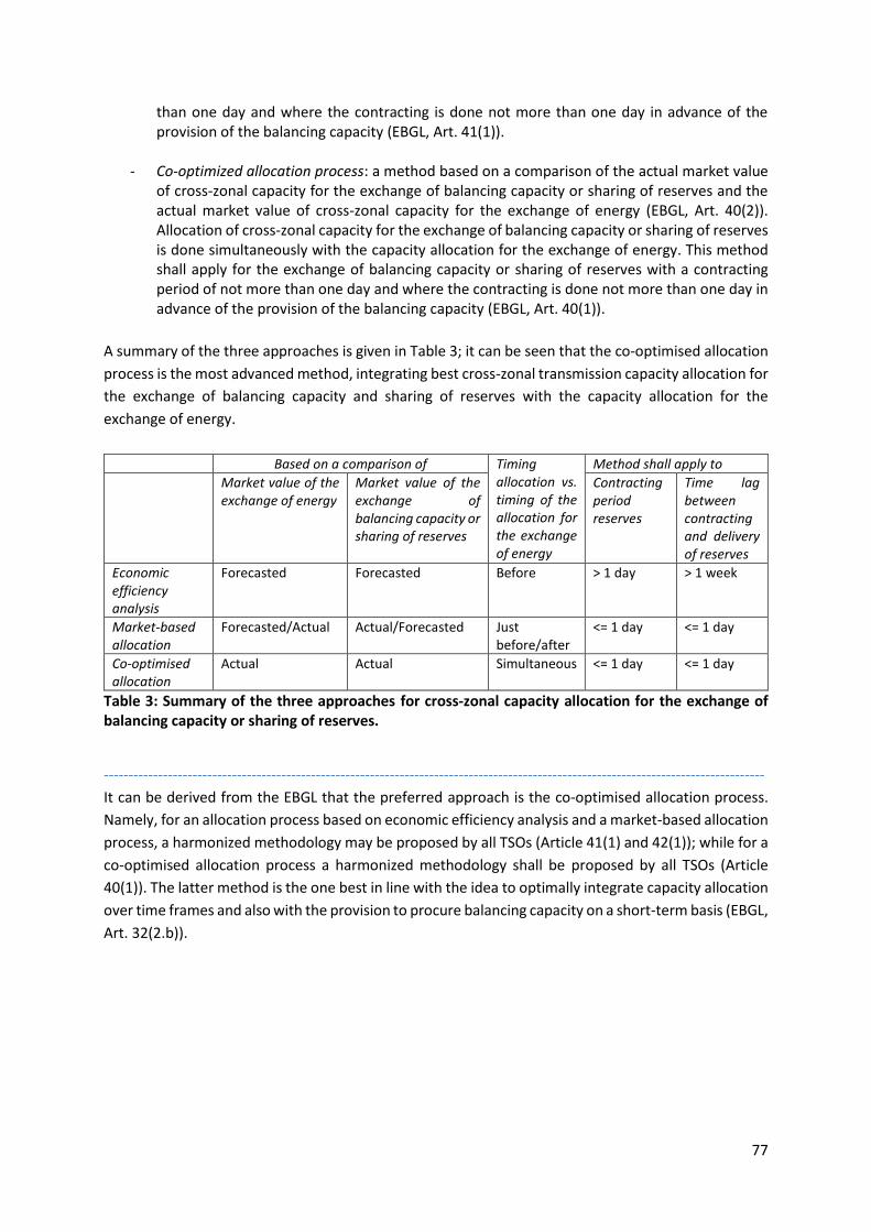
77
than one day and where the contracting is done not more than one day in advance of the provision of the balancing capacity (EBGL, Art. 41(1)).
- Co-optimized allocation process: a method based on a comparison of the actual market value of cross-zonal capacity for the exchange of balancing capacity or sharing of reserves and the actual market value of cross-zonal capacity for the exchange of energy (EBGL, Art. 40(2)). Allocation of cross-zonal capacity for the exchange of balancing capacity or sharing of reserves is done simultaneously with the capacity allocation for the exchange of energy. This method shall apply for the exchange of balancing capacity or sharing of reserves with a contracting period of not more than one day and where the contracting is done not more than one day in advance of the provision of the balancing capacity (EBGL, Art. 40(1)).
A summary of the three approaches is given in Table 3; it can be seen that the co-optimised allocation
process is the most advanced method, integrating best cross-zonal transmission capacity allocation for
the exchange of balancing capacity and sharing of reserves with the capacity allocation for the
exchange of energy.
Based on a comparison of Timing allocation vs. timing of the allocation for the exchange of energy
Method shall apply to
Market value of the exchange of energy
Market value of the exchange of balancing capacity or sharing of reserves
Contracting period reserves
Time lag between contracting and delivery of reserves
Economic efficiency analysis
Forecasted Forecasted Before > 1 day > 1 week
Market-based allocation
Forecasted/Actual Actual/Forecasted Just before/after
<= 1 day <= 1 day
Co-optimised allocation
Actual Actual Simultaneous <= 1 day <= 1 day
Table 3: Summary of the three approaches for cross-zonal capacity allocation for the exchange of balancing capacity or sharing of reserves.
--------------------------------------------------------------------------------------------------------------------------------------
It can be derived from the EBGL that the preferred approach is the co-optimised allocation process.
Namely, for an allocation process based on economic efficiency analysis and a market-based allocation
process, a harmonized methodology may be proposed by all TSOs (Article 41(1) and 42(1)); while for a
co-optimised allocation process a harmonized methodology shall be proposed by all TSOs (Article
40(1)). The latter method is the one best in line with the idea to optimally integrate capacity allocation
over time frames and also with the provision to procure balancing capacity on a short-term basis (EBGL,
Art. 32(2.b)).
78
Bibliography
ACER, 2016. Decision of ACER No 06/2016 on the electricity transmission system operators’ proposal for the determination of capacity calculation regions.
ACER, 2015a. List of NEMO designations [WWW Document]. URL http://www.acer.europa.eu/en/electricity/FG_and_network_codes/CACM/Pages/NEMO-Designations.aspx
ACER, 2015b. ACER Recommendation No 03/2015 on the Network Code on Electricity Balancing.
ACER, 2015c. ACER path towards the balancing market integration. Present. Balanc. Stakehold. Gr. 27/11/2015.
ACER, 2015d. ACER path towards the balancing market integration. Present. Balanc. Stakehold. Gr. 27/11/2015.
ACER, 2015e. ACER Opinion No 09/2015 on the compliance of NRAs’ decisions approving methods of cross-border capacity allocation in the CEE region.
ACER, 2013. Loop Flows Workshop - High-Level Conclusions.
ACER/CEER, 2016. Annual Report on the Results of Monitoring the Internal Electricity Markets in 2015.
ACER, ENTSOE, 2012. Regulatory framework for cross- border redispatching and countertrading. Present. Florence Forum.
AGORA, 2016. Refining Short-Term Electricity Markets to Enhance Flexibility. Stock. as well as Options Reform Pentalateral Energy Forum Reg.
Ausubel, L., Cramton, P., 2002. Demand Reduction and Inefficiency in Multi-Unit Auctions. Work. Pap. Univ. Maryl. doi:10.1093/restud/rdu023
Batlle, C., Mastropietro, P., Gómez-Elvira, R., 2014. Toward a Fuller Integration of the EU Electricity Market: Physical or Financial Transmission Rights? Electr. J. 27, 8–17. doi:10.1016/j.tej.2013.12.001
Bellenbaum, J., Bucksteeg, M., Kallabis, T., Pape, C., Weber, C., 2014. Intra-day cross-zonal capacity pricing. Study on behalf of Ofgem.
Benjamin, R., 2010. A further inquiry into FTR properties. Energy Policy 38, 3547–3556. doi:10.1016/j.enpol.2010.02.032
Brijs, T., De Jonghe, C., Hobbs, B.F., Belmans, R., 2017. Interactions between the design of short-term electricity markets in the CWE region and power system flexibility. Appl. Energy 195, 36–51. doi:10.1016/j.apenergy.2017.03.026
Brunekreeft, G., 2015. Empirics of Intraday and Real-time Markets in Europe: The Netherlands.
Chao, H., Peck, S., 1996. A market mechanism for electric power transmission. J. Regul. Econ. 10, 25–29.
Chaves-Ávila, J.P., Fernandes, C., 2015. The Spanish intraday market design: A successful solution to balance renewable generation? Renew. Energy 74, 422–432. doi:10.1016/j.renene.2014.08.017
Chaves-Ávila, J.P., van der Veen, R.A.C., Hakvoort, R.A., 2014. The interplay between imbalance pricing mechanisms and network congestions - Analysis of the German electricity market. Util. Policy 28,
79
52–61. doi:10.1016/j.jup.2013.11.005
Dijk, J., Willems, B., 2011. The effect of counter-trading on competition in electricity markets. Energy Policy 39, 1764–1773. doi:10.1016/j.enpol.2011.01.008
Doorman, G.L., Van Der Veen, R., 2013. An analysis of design options for markets for cross-border balancing of electricity. Util. Policy 27, 39–48. doi:10.1016/j.jup.2013.09.004
E-Bridge, IAEW, 2016. Impact of merit order activation of automatic Frequency Restoration Reserves and harmonised Full Activation times. Study on behalf of ENTSO-E.
E-Brige Consulting, 2014. Potential cross-border balancing cooperation between the Belgian , Dutch and German electricity Transmission System Operators.
Elia, 2017. Marktwerkingsregels voor de compensatie van de kwartuuronevenwichten - Inwerkingstreding volgend op de beslissing van de CREG (B) 1632 van 06/07/2017.
Elia, TenneT, 2014. Design of a Harmonised Reactive Balancing Market with Cross Zonal Optimisation of Frequency Restoration between LFC Blocks. TenneT Elia Final Rep. step 2 XB Balanc. Proj. BE-NL 1–111.
Elia, TenneT, KEMA, 2013. Cross-Border Exchange of Balancing Energy and Operational Reserves : Benefits and Issues. Potential Cross-Border Balanc. Coop. between Elia Tennet. Presenation a Stakehold. Work. Brussels.
ENTSO-E, 2017a. Time to team up and create value - presentation by Bente Hagem on the network code conference (4 May 2017).
ENTSO-E, 2017b. Regional Security Coordinators [WWW Document]. URL https://www.entsoe.eu/major-projects/RSC/Pages/default.aspx
ENTSO-E, 2017c. All TSOs ’ proposal for harmonised allocation rules for long-term transmission rights in accordance with Article 51 of FCA GL.
ENTSO-E, 2017d. All TSOs ’ proposal for the establishment of a Single Allocation Platform ( SAP ) in accordance with Article 49 and for the cost sharing methodology in accordance with Article 59 of FCA GL.
ENTSO-E, 2017e. Report on the progress and potential problems with the implementation of Single Day- Ahead and Intraday Coupling.
ENTSO-E, 2017f. All TSOs’ proposal for the single methodology for pricing intraday cross-zonal capacity in accordance with Article 55 of CACM.
ENTSO-E, 2017g. Survey on ancillary services procurement, balancing market design 2016. Present. by ENTSO-E Work. Gr. Ancillary Serv.
ENTSO-E, 2017h. Cross Border Electricity Balancing Pilot Projects [WWW Document]. URL https://www.entsoe.eu/major-projects/network-code-implementation/cross-border-electricity-balancing-pilot-projects/Pages/default.aspx
ENTSO-E, 2017i. Balancing code early implementation: TSOs consult on the TERRE pilot project [WWW Document]. URL https://www.entsoe.eu/news-events/announcements/announcements-archive/Pages/News/balancing-code-early-implementation-TSOs-consult-on-the-TERRE-pilot-project.aspx

80
ENTSO-E, 2017j. Imbalance netting [WWW Document]. URL https://www.entsoe.eu/major-projects/network-code-implementation/electricity-balancing/igcc/Pages/default.aspx
ENTSO-E, 2017k. Regional groups [WWW Document]. URL https://www.entsoe.eu/about-entso-e/system-operations/regional-groups/Pages/default.aspx
ENTSO-E, 2016. Activation purposes of Balancing Energy bids - Draft version 5. WG Ancillary Serv. – SG Act. Purp.
ENTSO-E, 2015a. All TSOs’ proposal for Capacity Calculation Regions (CCRs) in accordance with Article 15(1) of the CACM GL.
ENTSO-E, 2015b. Capacity Calculation Regions [WWW Document]. URL https://consultations.entsoe.eu/system-operations/capacity-calculation-regions/consult_view/
ENTSO-E, 2015c. Survey on Ancillary services procurement, Balancing market design 2014 [WWW Document]. URL https://www.entsoe.eu/Documents/Publications/Market Committee publications/150127_WGAS_Survey_2014.pdf
ENTSO-E, 2014a. ENTSO-E Policy Paper Future TSO Coordination for Europe.
ENTSO-E, 2014b. Supporting Document for the Network Code on Operational Planning and Scheduling.
Frunt, J., 2011. Analysis of balancing requirements in future sustainable and reliable power systems. TU Eindhoven.
FSR, 2014. Electricity markets ( principles ). CEER-FSR Train. Introd. to Fundam. Energy Regul.
FTI-Compass Lexecon, 2016. Options for the future of power system regional coordination. Rep. ENTSO-E.
Genoese, F., Drabik, E., Egenhofer, C., 2016. The EU power sector needs long-term price signals. CEPS Spec. Rep. No. 135.
Glachant, J.M., 2016. Taking stock of the EU Power Target Model’’... and steering its future course. Energy Policy 96, 673–679. doi:10.1016/j.enpol.2016.03.010
Glachant, J.M., Lévêque, F., 2006. Electricity Reform in Europe: Towards a Single Energy Market. Edward Elgar.
Glachant, J.M., Pignon, V., 2005. Nordic congestion’s arrangement as a model for Europe? Physical constraints vs. economic incentives. Util. Policy 13, 153–162. doi:10.1016/j.jup.2004.12.009
Gorecki, P.K., 2013. Ensuring compatibility of the all-island electricity system with the target model: Fitting a square peg into a round hole? Energy Policy 52, 677–688. doi:10.1016/j.enpol.2012.10.028
Haberg, M., Doorman, G., 2016. Classification of balancing markets based on different activation philosophies: Proactive and reactive designs. Int. Conf. Eur. Energy Mark. EEM 2016–July. doi:10.1109/EEM.2016.7521272
Hagemann, S., Weber, C., 2015. Trading Volumes in Intraday Markets - Theoretical Reference Model and Empirical Observations.
Haucap, J., Heimeshoff, U., Jovanovic, D., 2014. Competition in germany’s minute reserve power market: An econometric analysis. Energy J. 35, 137–156. doi:10.5547/01956574.35.2.7
81
Henriot, A., 2014. Market design with centralized wind power management: handling low-predictability in intraday markets. Ene 35, 99–117. doi:10.2139/ssrn.2481918
Henriot, A., Glachant, J.M., 2013. Melting-pots and salad bowls: The current debate on electricity market design for integration of intermittent RES. Util. Policy 27, 57–64. doi:10.1016/j.jup.2013.09.001
Hiroux, C., Saguan, M., 2010. Large-scale wind power in European electricity markets: Time for revisiting support schemes and market designs? Energy Policy 38, 3135–3145. doi:10.1016/j.enpol.2009.07.030
Hirth, L., Ziegenhagen, I., 2015. Balancing Power and Variable Renewables: Three Links. Renew. Sustain. Energy Rev. 50, 1035–1051. doi:10.1016/j.rser.2015.04.180
Hogan, W.W., 2013. Electricity Scarcity Pricing Through Operating Reserves. Econ. Energy Environ. Policy 2, 65–86. doi:10.5547/2160-5890.2.2.4
Hogan, W.W., 1992. Contract networks for electric power transmission. J. Regul. Econ. 4, 211–242.
Joskow, P., Tirole, J., 2000. Transmission Rights and Market Power on Electric Power Networks. RAND J. Econ. 31, 450–487.
Just, S., Weber, C., 2015. Strategic behavior in the German balancing energy mechanism: incentives, evidence, costs and solutions. J. Regul. Econ. 48, 218–243. doi:10.1007/s11149-015-9270-6
Kahn, A.E., Cramton, P.C., Porter, R.H., Tabors, R.D., 2001. Uniform Pricing or Pay-as-Bid Pricing. Electr. J. 14, 70–79. doi:10.1016/S1040-6190(01)00216-0
Kristiansen, T., 2007. Cross-border transmission capacity allocation mechanisms in South East Europe. Energy Policy 35, 4611–4622. doi:10.1016/j.enpol.2007.03.020
Kunz, F., Zerrahn, A., 2016. Coordinating cross-country congestion management: Evidence from Central Europe. Energy J. 37, 32. doi:10.5547/01956574.37.SI3.fkun
Levin, T., Botterud, A., 2015. Electricity market design for generator revenue sufficiency with increased variable generation. Energy Policy 87, 392–406. doi:10.1016/j.enpol.2015.09.012
Littlechild, S., 2015. Reflections on cash-out arrangements. Lett. to 1Roger Witcomb 1–13.
Littlechild, S., 2007. Electricity Cash Out Arrangements.
Marneris, I.G., Biskas, P.N., 2015. Integrated Scheduling Model for Central Dispatch systems in Europe. 2015 IEEE Eindhoven PowerTech, PowerTech 2015 1–6. doi:10.1109/PTC.2015.7232641
Mastropietro, P., Rodilla, P., Batlle, C., 2015. The unfolding of regional electricity markets: measures to improve the firmness of cross-border trading. IIT Work. Pap. IIT-14-160A.
Meeus, L., 2011. Why (and how) to regulate power exchanges in the EU market integration context? Energy Policy 39, 1470–1475. doi:10.1016/j.enpol.2010.12.019
Meeus, L., Belmans, R., 2007. Is the prevailing wholesale market design in Europe and North America comparable? 2007 IEEE Power Eng. Soc. Gen. Meet. PES. doi:10.1109/PES.2007.385523
Meeus, L., Purchala, K., Belmans, R., 2005. Development of the internal electricity market in Europe. Electr. J. 18, 25–35. doi:10.1016/j.tej.2005.06.008

82
Meeus, L., Verhaegen, K., Belmans, R., 2009. Block order restrictions in combinatorial electric energy auctions. Eur. J. Oper. Res. 196, 1202–1206. doi:10.1016/j.ejor.2008.04.031
Mott MacDonald, 2013. Impact Assessment on European Electricity Balancing Market. Rep. EC. Contract EC DG ENER/B2/524/2011.
Müsgens, F., Neuhoff, K., 2006. Modelling Dynamic Constraints in Electricity Markets and the Costs of Uncertain Wind Output. Energy.
Müsgens, F., Ockenfels, A., Peek, M., 2014. Economics and design of balancing power markets in Germany. Int. J. Electr. Power Energy Syst. 55, 392–401. doi:10.1016/j.ijepes.2013.09.020
Nabe, C., Neuhoff, K., 2015. Intraday- and real time activity of TSOs: Germany. DIW Res. Rep.
Neuhoff, K., Batlle, C., Brunekreeft, G., Konstantinidis, C.V., Nabe, C., Oggioni, G., Rodilla, P., Schwenen, S., Siewierski, T., Strbac, G., 2015a. Flexible Short-Term Power Trading: Gathering Experience in EU Countries. Discuss. Pap. 1494. doi:10.13140/RG.2.1.1578.1609
Neuhoff, K., Richstein, J., 2016. Coordinated Balancing of the European Power System. Res. Rep.
Neuhoff, K., Richstein, J., May, N., 2016a. Auctions for intraday- Trading impacts on efficient power markets and secure system operation. DIW Res. Rep.
Neuhoff, K., Ritter, N., Salah-Abou-El-Enien, A., Vassilopoulos, P., 2016b. Intraday markets for power: Discretizing the continuous trading? DIW Discuss. Pap. No. 1544.
Neuhoff, K., Ritter, N., Schwenen, S., 2015b. Bidding Structures and Trading Arrangements for Flexibility across EU Power Markets. Rep. from Futur. Power Mark. Work. 2015, held Ofgem, London, June 26. doi:10.1007/s10273-011-1262-2
Neuhoff, K., Schwenen, S., 2013. Beyond gate closure. 2nd Rep. Futur. Power Mark. Work. DIW Berlin.
Neuhoff, K., Wolter, S., Schwenen, S., 2016c. Power markets with renewables: New perspectives for the European Target Model. Energy J. 37, 23–38. doi:10.5547/01956574.37.2.kneu
Newbery, D., 2016. Missing money and missing markets: Reliability, capacity auctions and interconnectors. Energy Policy 94, 401–410. doi:10.1016/j.enpol.2015.10.028
Newbery, D., 2006. Market design. CWPE 0615 EPRG 0515.
Ocker, F., Ehrhart, K.M., 2017. The German Paradox’’ in the balancing power markets. Renew. Sustain. Energy Rev. 67, 892–898. doi:10.1016/j.rser.2016.09.040
Ofgem, 2015. Balancing and Settlement Code (BSC) P305: Electricity Balancing Significant Code Review Developments.
Ofgem, 2014. Bidding Zones Literature Review.
OMIE, 2015. Corporate report 2015.
Papavasiliou, A., Smeers, Y., 2017. Remuneration of Flexibility using Operating Reserve Demand Curves: A Case Study of Belgium. Energy J. Forthcomin. doi:10.5547/01956574.38.6.apap
PCR, 2016. EUPHEMIA: Description and functioning (July 2016).
Pentalateral Energy Forum, 2016. Balancing. Penta Flex. Work stream – Penta SG3 – Tech. Backgr. Pap. - Balanc.
83
Pérez-Arriaga, I.J., 2013. Regulation of the Power Sector. Springer.
Pérez-Arriaga, I.J., Rubio, F.J., Puerta, J.F., Arceluz, J., Marin, J., 1995. Marginal pricing of transmission services: An analysis of cost recovery. IEEE Trans. Power Syst. 10, 546–553. doi:10.1109/59.373981
PJM, 2011. Energy Markets - FTRs & ARRs. Presentation for the Interconnection Training Program- Module EM6.
Plancke, G., De Vos, K., De Jonghe, C., Belmans, R., 2016. Efficient use of transmission capacity for cross-border trading: Available Transfer Capacity versus flow-based approach. IEEE Int. Energy Conf. ENERGYCON. doi:10.1109/ENERGYCON.2016.7513974
Rakhmah, T.F., Yanfei, L., 2016. A review on Institutional Framework , Principles , and Key Elements for Integrated Electricity Market : Implications for ASEAN. ERIA Discuss. Pap. Ser. ERIA-DP-2016-26.
Regelleistung.net, 2017. Grid Control Cooperation [WWW Document]. Internetplattform zur Vergabe von Regelleistung. URL https://www.regelleistung.net/ext/static/gcc?lang=en
Rodilla, P., Batlle, C., 2015. Empirics of Intraday and Real-time Markets in Europe: Spain.
Schavemaker, P.H., Beune, R.J.L., 2013. Flow-based market coupling and bidding zone delimitation: Key ingredients for an efficient capacity allocation in a zonal system. Int. Conf. Eur. Energy Mark. EEM. doi:10.1109/EEM.2013.6607366
Spodniak, P., Collan, M., Makkonen, M., 2017. On long-term transmission rights in the Nordic electricity markets. Energies 10, 1–19. doi:10.3390/en10030295
TenneT, Elia, 50Hz, APG, Amperion, Transnet BW, 2016. EXPLORE: Target model for exchange of frequency restoration reserves.
TGE, 2015. Polish Power Exchange (TGE) Becomes a Member of the European Multi-Regional Coupling (MRC) Market [WWW Document]. URL https://www.tge.pl/en/27/news/611/polish-power-exchange-tge-becomes-a-member-of-the-european-multi-regional-coupling-mrc-market
Van den Bergh, K., Boury, J., Delarue, E., 2016. The Flow-Based Market Coupling in Central Western Europe: Concepts and definitions. Electr. J. 29, 24–29. doi:10.1016/j.tej.2015.12.004
Van den Bergh, K., Bruninx, K., Delarue, E., 2017. Cross-border reserve markets : network constraints in cross-border reserve procurement. TME Work. Pap. - Energy Environ. Last Updat. April 2017.
Van den Bergh, K., Couckuyt, D., Delarue, E., D’Haeseleer, W., 2015. Redispatching in an interconnected electricity system with high renewables penetration. Electr. Power Syst. Res. 127, 64–72. doi:10.1016/j.epsr.2015.05.022
Van Hertem, D., Ghandhari, M., 2010. Multi-terminal VSC HVDC for the European supergrid: Obstacles. Renew. Sustain. Energy Rev. 14, 3156–3163. doi:10.1016/j.rser.2010.07.068
Vandezande, L., 2011. Design and integration of balancing markets in Europe. PhD Thesis - KU Leuven.
Vandezande, L., Meeus, L., Belmans, R., Saguan, M., Glachant, J.M., 2010. Well-functioning balancing markets: A prerequisite for wind power integration. Energy Policy 38, 3146–3154. doi:10.1016/j.enpol.2009.07.034
Verpoorten, K., Jonghe, C. De, Delarue, E., Belmans, R., 2016. Reservation of interconnection capacity for imbalance netting : case for the Belgian-Dutch border. Work. Pap. KU Leuven.

84
Wikiwand, 2017. Deutsches Übertragungsnetz von 50Hertz, Amprion, EnBW und TenneT [WWW Document]. URL http://www.wikiwand.com/de/Regelleistung_(Stromnetz)