The Estimation of Measurement Uncertainty of Small ... Arc Analysis - NIST.pdfThe Estimation of...

1

The Estimation of Measurement Uncertainty of Small Circular Features

Measured by Coordinate Measuring Machines

S.D. Phillips, B. Borchardt, and W.T. Estler

National Institute of Standards and Technology

and

John Buttress

Hutchinson Technology Inc.

Key Words: CMM, Uncertainty, Probe, Sampling Strategy, Circle

Abstract

This paper examines the measurement uncertainty of small circular features as a function of the sampling

strategy, i.e., the number and distribution of measurement points. Specifically, we examine measuring a

circular feature using a three-point sampling strategy in which the angular distance between the points

varies from widely spaced, 120°, to closely grouped, a few degrees. Both theoretical and experimental

results show that the measurement uncertainty is a strong function of the sampling strategy. The

uncertainty is shown to vary by four orders of magnitude as a function of the angular distribution of the

measurement points. A conceptual framework for theoretically estimating the measuring uncertainty is

described and a good agreement with experiment is obtained when the measurements are consistent with

the assumptions of the theoretical model. This paper is an expansion of a previous internal report1 with

additional material on analog probes and probe lobing models.

2

Introduction

The determination of measurement uncertainty of coordinate measuring machines (CMMs) is a complex

and daunting task. The very versatility that allows CMMs to inspect a wide range of features and part

types makes evaluating the measurement uncertainty a multifaceted problem. Currently the vast majority

of CMM measurements have no rigorous uncertainty budget. This is not to say that these measurements

are significantly in error, but rather that their uncertainty is usually a guess based on the experience of the

operator. While an experienced operator may often have a reasonable feeling for the capability of a

CMM, there are measurement situations where intuition and experience may dramatically fail.

Although aspects of the variation in feature parameters as a function of sampling strategy have been

previously investigated,2,3 in this paper we evaluate the measurement uncertainty using the terminology

and methodology recommended by the International Committee for Weights and Measures (CIPM)4.

This terminology has been adopted by the International Organization for Standardization (ISO) and by

national laboratories including NIST5. This methodology states that the uncertainty of a measurement

result y can be quantified by the combined standard uncertainty uc, given below. In this expression the

measurand Y (the quantity being measured), is dependent on a number of different sources of uncertainty

Xi (i = 1 to N).

Y = f (X1, X2,...,XN ) (1)

u fx

u x fx

fx

u x xii

N

iij i

N

i

N

ji jc

2

1

22

11

1

2=FHGIKJ +

= = +=

−

∑ ∑∑∂∂

∂∂

∂∂

( ) ,d i (2)

This equation (loosely speaking) states that the combined uncertainty (characterized by its variance uc2 )

is the summation of each individual uncertainty source (characterized by its variance u2(xi)), multiplied by

3

the square of a quantity known as the sensitivity coefficient (denoted ∂f/∂xi) whose magnitude describes

the importance of the uncertainty source relative to the total measurement uncertainty. The quantity u(xi,

xj) is the covariance of xi and xj, and is a measure of the correlation between these two uncertainty

sources. The combined standard uncertainty, uc, can be thought of as representing one standard deviation

of the measurement uncertainty resulting from combining all known sources of uncertainties in the

manner described by eq. (2).

Although eq. (2) describes the method of determining the combined standard uncertainty, the real work is

in quantifying the sources of uncertainty by a variance, determining the correlation between these

uncertainty sources, and in evaluating the sensitivity coefficients. Exactly how the measurement

uncertainty sources are decomposed can depend on the specific measurement under investigation and the

methods available to quantify the uncertainty sources. One general paradigm for separating CMM

uncertainty sources is shown in Fig. 1.

For the problem we are considering in this paper, namely the measurement of a small ring gauge, many of

the factors shown in Fig. 1 can be neglected. For example, since the form error of the ring gauge is on the

order of 0.2 µm, the contribution to the combined standard uncertainty due to part form error is

insignificant with respect to other sources of error. Furthermore, since the sampling strategy used

involves only three points, the algorithm selection and implementation issues are rendered moot since

three points exactly determine a circle and the problem becomes analytic. (However, tests were

performed to ensure that other errors, such as the internal representation of numbers resulting in round off

error, were insignificant.) Similarly, extrinsic factors were carefully controlled to minimize their effect

on the measurement result. Consequently, determining the combined standard uncertainty in our ring

gauge measurements reduces to evaluating the uncertainty in the CMM and then determining the

appropriate sensitivity coefficient for the particular sampling strategy used in the measurement. Since the

4

aggregate of the CMM hardware errors manifest themselves as errors in the coordinates of the individual

measurement points, conceptually the problem reduces to that shown in Fig. 2.

Experimental Estimation of Uncertainty

The measurement uncertainty of a small ring gauge (having a diameter of 47 mm (1.85 in)) can be

estimated directly by repeated measurements in which parameters that are not strictly controlled during a

normal part inspection are allowed to vary. (This is somewhat analogous to gauge repeatability and

reproducibility studies in which factors such as changing the CMM operator can result in increased

measurement variation.) In order to focus the scope of our investigation, we have minimized other factors

such as operator variation (by using a computer controlled CMM), precisely specifying the sampling

strategy, and employing a nearly perfect ring gauge. We do, however, vary the orientation of the

sampling strategy coordinate system with respect to the machine coordinate system as discussed below.

The quantity of interest is the measurement variation (a direct indication of measurement uncertainty) of

each specified three-point sampling strategy, where the sampling strategy is defined by specifying the

angle θ shown in Fig. 3.

The measurement procedure is to define a coordinate system with the origin at the center of the ring

gauge and the X and Y axes initially aligned along the machine coordinate system. The ring gauge is

measured using the sampling strategy shown in Fig. 3, i.e., the three measurement points are

symmetrically displaced with respect to the Y axis. The values of the radius and the X and Y circle center

location are recorded. The coordinate system is then rotated about the origin by ten degrees with respect

to the machine coordinate system, and the measurement repeated. This process is repeated a total of 36

times so that the sampling strategy and the defined coordinate system have been incremented in 10 degree

steps around the entire ring gauge. Note that since the sampling strategy and defined coordinate system

rotate together with respect to the machine coordinate system the sampling strategy is always identical to

Fig. 3, i.e., the points are always symmetrically displaced with respect to the defined Y axis. This

5

definition of the sampling strategy (symmetric with respect to the Y axis) will lead to different

measurement results in X and Y circle center coordinates. Using the resulting 36 values of the ring gauge

radius and center location, the standard deviation of each of these quantities is then computed. The entire

process is repeated again for a different sampling strategy, i.e., a different value of θ. The final result can

be shown as a plot of the standard deviation of the fitted parameters (radius and center location) versus θ

(which defines the sampling strategy) (see for example Fig. 4). Since different stylus lengths and probe

types behave differently, the procedure was repeated for several common probe configurations. Although

a complete uncertainty analysis of this measurement would include additional sources of uncertainty, e.g.,

the thermal expansion of the gauge and the uncertainty in the effective stylus size, these factors can be

accounted for in a straightforward manner. (These factors are independent of the sampling strategy and

their uncertainty would be added in the usual (RSS) manner to the calculation of the combined standard

uncertainty.)

Although it may seem unrealistic to inspect a ring gauge using points which are closely grouped together,

there are many measurement situations where only a small partial arc of material is present which forces

this situation. In such a partial arc case it will be shown that the uncertainty of the usual circle

measurement is very large and that an alternative may be needed, such as fixing one of the circle

parameters to its nominal value, or redefining the partial arc as a profile tolerance.

Theoretical Estimates of Uncertainty

One benefit of a theoretical model of measurement uncertainty is that it allows one to avoid the large

number of measurements required to estimate the measurement uncertainty experimentally. Such

measurements are both time consuming and costly, and may require a skilled metrologist to design the

procedure. Using a theoretical model of the uncertainty allows the operator to determine the uncertainty

directly, for example using a handbook, formula, or software program. Any theoretical model must

contain two basic components, first an estimation of the uncertainty of the coordinates of each

6

measurement point, and secondly a method to propagate the point coordinate uncertainty into the

uncertainty of the substitute geometry, e.g., the radius and center coordinates for the ring gauge.

A sophisticated model for determining the point coordinate uncertainty may include a detailed description

of the machine. For example, all of the rigid body motion parameters (three translational and three

rotational for each axis) may each have an associated uncertainty and their effects would propagate

through to each measurement point. Similarly, other effects from causes such as nonrigid body behavior,

hysteresis, thermally induced errors, and so forth, could also be included to describe the uncertainty of the

CMM. Such a model would have a different value of uncertainty at each point in the CMM work zone,

and in general, a different uncertainty for each coordinate (x, y, and z) at each point. The advantage of

this approach is the ability to predict precisely the point coordinate uncertainty throughout the workzone.

The disadvantage is the difficulty of developing a detailed model of the CMM and of the measurements

needed to evaluate the model parameters. Additionally, the model parameters must be temporally stable

or the predictions will degrade as the parameters drift from their assessed values. Additional aspects of

estimating CMM measurement uncertainty can be found in reference 6.

For the measurement of a ring gauge, which is considered in this paper, most of the long range, i.e.,

length dependent, sources of uncertainty can be neglected because the ring gauge has a very small

diameter. Consequently, we focus on those errors which are short range, such as the system repeatability

and the errors associated with the probe mechanism. Specifically, we will demonstrate two probe models,

one assuming independent and identically distributed errors which can be characterized by a single

parameter, and a second probe model which includes correlated errors characteristic of the probe's

internal structure.

Single Parameter Model: A simple model of the system can be characterized by a single parameter to

describe the CMM point coordinate uncertainty. This means that each point within the CMM workzone

7

has the same uncertainty, and that these points are independent of one another, i.e., their uncertainty is not

correlated. Similarly, each coordinate (x, y, and z) of every point also has this same value of uncertainty.

Obviously, use of a single number to represent the uncertainty of the CMM is a tremendous over

simplification; nevertheless in some cases the results can be surprisingly good.

To estimate the value of this single parameter, which must be stated as a variance (or as a standard

deviation) when using the CIPM formulation, we take the standard deviation of the radial residuals found

from the ASME B89.4.1 point-to-point probe performance test7. In this procedure 49 points are recorded

on the surface of a small high precision sphere and a (least squares) best fit to a sphere is calculated. The

radial residuals to each of the measurement points from the best fit radius are determined and their

standard deviation is used for the single parameter to characterize the point coordinate uncertainty of the

CMM. The sphere used in this measurement has a form error of less than 0.15 µm8, and hence this error

is negligible compared to the probe errors. Although this procedure is conducted on a small sphere, one

can imagine its diameter shrinking to zero and the result being 49 measurements of the same (physical)

point, with the standard deviation of these 49 values being characteristic of the uncertainty of the point.

The advantage of this method is that many CMM users know about the B89 point-to-point probe

performance test and, hence, can easily perform the test to determine this value. As previously

mentioned, such a simple model of the CMM will not accurately predict the uncertainty for all possible

CMM measurements.

For the special case of a circle measured using a three-point sampling strategy the problem is analytic and

allows a direct calculation of the substitute geometry uncertainty given by eq. (3), assuming that the

errors at each of the three points are independent, i.e., are not correlated. Therefore we can write down

directly the combined standard uncertainty for each of the substitute geometry parameters as shown in

eq. (3) as follows9:

8

Radius: u uc2

B892cos

cos=

+−

+1 2

2 1

2

2

θθ( )

...

Y center: u uc2

B892

cos=

−+

32 1 2( )

...θ

(3)

X center: u uc2

B892= +

12 2sin

...θ

where u2B89 is the variance of the radial residuals found from the B89.4.1 point-to-point probe

performance test and +... indicates that other sources of uncertainty should be included in the combined

standard uncertainty. However, we are not explicitly considering them in this paper. Note that the form

of eq. (3) is that of eq. (2) where the trigonometric function (describing the sampling strategy) plays the

role of the sensitivity coefficient and the magnitude of the uncertainty source is characterized by the

variance of the fit residuals, i.e., u2B89. It is worth noting for the sampling strategies considered (depicted

in Fig. 3), that in the limit of small θ, the variance of both the radius and Y center parameters approach

the same limiting value of 6/θ 4.

Single Parameter Model Results: We have estimated the uncertainty for the measurement of a small

ring gauge using the single parameter model. In order to examine the generality of the procedure we have

considered several different probes and stylus combinations. For all the probes we examined we

estimated the variance of the uncertainty source using the B89 point-to-point probe performance test. To

accurately estimate this variance we have repeated the B89 probe test a total of 10 times and used the

mean of the results as the characteristic value. Table 1 presents the B89 results for the six probe

configurations used in our study10.

Figures 4 to 9 show measurement uncertainty of the ring gauge as a function of sampling strategy

determined experimentally and theoretically, using the single parameter model, for the first six probe

configurations given in Table 1. This includes the cases of a high accuracy analog probe (used in a

9

discrete point data collection mode), a piezoelectric base touch trigger probe (which triggers from the

impact of the stylus with the part), and several different configurations of the ubiquitous mechanically

based touch trigger probe. The experimental results are the standard deviations of the 36 measurements

(each at a different probe approach direction) of the ring gauge for each sampling strategy. The

theoretical results are calculated using the values of standard deviation given in Table 1 and the sampling

strategy rules (which play the role of sensitivity coefficients) given by eq. (3). The ordinate of these plots

represents a single standard deviation. If an expanded uncertainty is required, then the uncertainty is

multiplied by the coverage factor which is typically two, i.e., twice the combined standard uncertainty.

Also plotted for reference is the value of the B89 derived standard deviation from Table 1.

The agreement between the experimentally determined standard deviation and that of the theoretically

predicted standard deviation using the single parameter model is reasonably good for many of the probe

configurations presented. It is clear that the sampling strategy plays an enormous role in the uncertainty.

Neglecting this effect would lead to an uncertainty prediction that would be a constant for all values of θ,

i.e., would predict a straight line with a magnitude equal to the standard deviation found from the B89

point-to-point probe performance test.

In the case of the piezoelectric (TP12) probe the agreement between the experimental and theoretical

results for the radial uncertainty is very good. We attribute this conformity to the fact that the

piezoelectric probe is dominated by random (not systematic) errors and consequently the assumption

implicit in the sampling strategy rules of independent uncorrected errors at each measurement point is

closely realized by this type of probe. The theoretical uncertainty tends to underestimate the variation in

the X and Y center location by a small amount. We believe this is caused by thermal drift which is

cumulative in the case of measuring the center location. This (and other) sources of uncertainty could

have been added to the theoretical model but are not explicitly considered here because they are not the

focus of this paper.

10

Similarly, the experimental results for the analog probe agree well with the uncertainty calculation using

the single parameter model. Although the internal mechanism of this probe involves numerous flexure

stages, the data show no evidence of this mechanism, i.e. there is no structure in the data curves that

cannot be accounted for by the single parameter model. With the exception of data from the probe lobing

correction model (discussed later), the analog probe is the only probe utilizing directionally dependent

compensation (as opposed to using a single value for an "effective stylus tip diameter", which is

omnidirectional). While the mechanical components of the probe head (e.g. flexure stages) are not error-

mapped, the directionally dependent deflection of the stylus is corrected through a transformation matrix

calculated using a 33-point calibration of a sphere. This is possible because the analog probe returns a

probing vector. Its "discrete point mode" is actually the result of an intercept of a linear regression using

approximately 25 points collected in a quasi-static state. This process effectively compensates for

systematic errors and the remaining small uncorrelated probing errors can be reasonably accounted for by

the single parameter model.

In many types of common touch trigger probes, e.g., TP2 and TP6, the mechanical structure supporting

the stylus also serves as the electrical switch which is triggered when the stylus is displaced. This class of

probes is known to have a directional sensitivity (discussed later) which increases with stylus length.

Consequently, two new aspects to the uncertainty curves are apparent: (1) there is some structure to the

experimental uncertainty curves in the region where θ is between 60° and 120°; (2) the single parameter

uncertainty model significantly overestimates the uncertainty for θ less than 10°. Both of these effects

are most pronounced in Fig. 9, which depicts the data from a 100 mm stylus probe. The failure of the

single parameter model to account for these effects is not surprising since the model is based on the

assumption of independent random errors at each measurement point, and for this class of touch trigger

probes (with a long stylus) the systematic directionally dependent probing errors are very significant.

11

Probe Lobing Model: A more sophisticated model of the point coordinate uncertainty could include the

systematic error behavior of the probe. This mechanism results in a directionally dependent sensitivity of

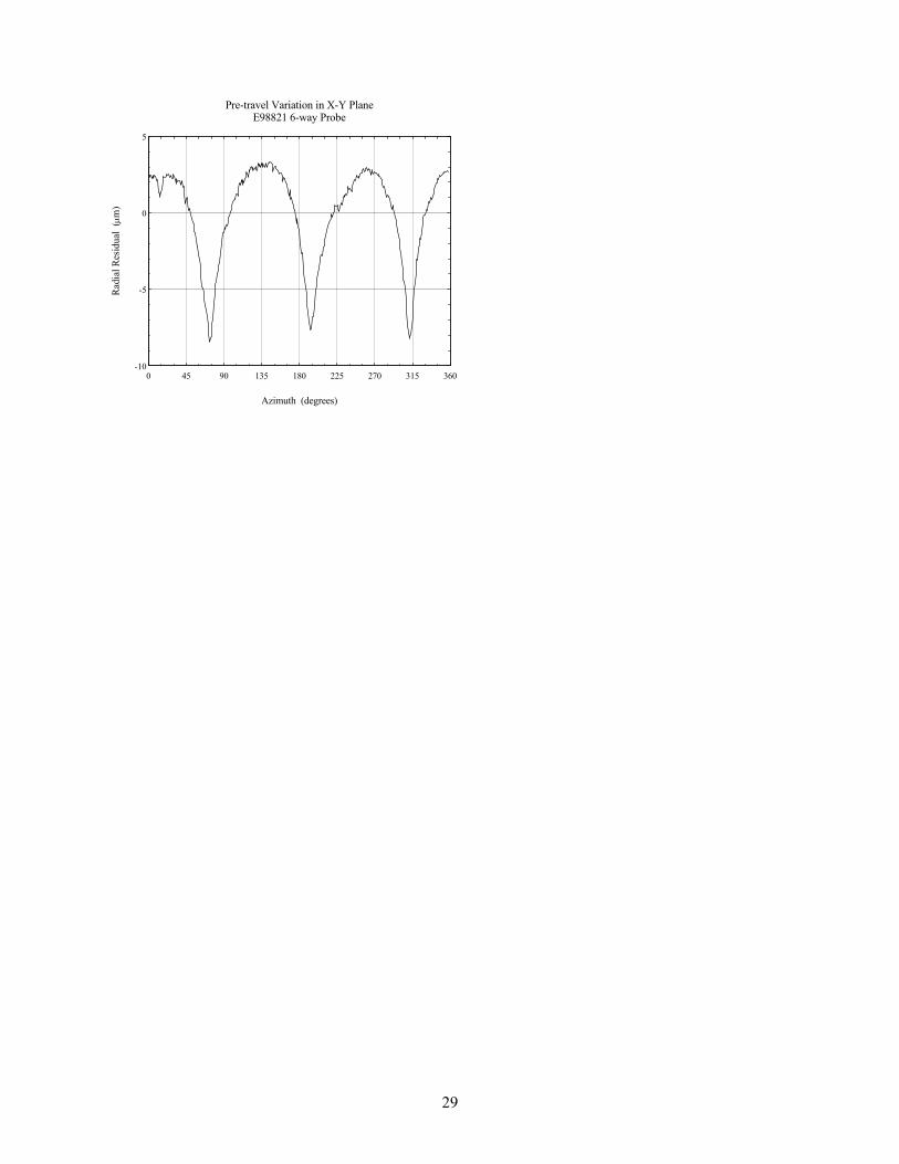
the probe, commonly called probe lobing. For most touch trigger probes the measurement of circular

parts appears to have a three-lobed shape, reflecting the triangular mechanical structure within the probe.

Figure 10 shows the three lobed pattern which is the result of this highly systematic error. For this class

of probes the error at any measurement point is highly dependent upon the probe approach direction and

hence for probe approach directions which are close together, the probing errors will be similar. A

description of the behavior of one lobe (valid for measurements in the XY plane as is the case with our

circle measurement) is given by the pre-travel function t(φ) shown in eq. (4) where φ is the probe

approach direction and α and γ are parameters characteristic of the probe and stylus under

consideration.11 The pre-travel function t(φ) can be combined with a small random error, representing the

system repeatability, to give a more complete description of the probe model.

t φ α φ φ γφ φ

b g b g b g= − +−

coscos0

0

(4)

The variation in the substitute geometry (center location and radius) from an error source described by eq.

(4) can be easily determined by direct numerical simulation. This procedure is preferred to an analytic

solution since each of the three probe lobes have the form of eq. (4), hence the pre-travel function is non-

differentiable at their joining points (corresponding to probe lobe cusps). For each ring gauge

measurement, eq. (4) (and its counterparts describing the other two lobes) is evaluated at three different

values of φ (successively incremented by an angle θ ) to obtain the point coordinate error at each of the

three measurement points, and the circle fit is performed. The arbitrary initial orientation of the probe,

given by φ0, is then incremented by a small amount and the procedure is repeated until φ

0 has completed

one full rotation. This is analogous to the experimental situation of clocking the probe orientation by 10°

a total of 36 times to sample over approximately all the possible probe orientations.

12

Probe Lobing Model Results: Figure 11 illustrates the application of a three-dimensional version11 of

eq. (4) applied to the 49 points taken on a sphere during the B89 point-to-point probe performance test.

The close agreement of the theoretical and experimental results demonstrates that the probe lobing model

can effectively account for most systematic errors in this class of probes. Applying this model, i.e., eq.

(4), to the same ring gauge measurement data shown in Fig. 9, yields Fig. 12. Note in particular, that this

model correctly accounts for the structure in the data curves and gives good agreement for the uncertainty

prediction in the region of small sampling angle. Alternatively, the probe lobing model can be used to

correct the individual points for the systematic pre-travel error during the measurement. The resulting

variation in the circle fits using the corrected measurement points is shown in Fig. 13, together with an

uncertainty prediction using the single parameter model. This corrected data fits well to the single

parameter model since the residual errors are reasonably consistent with the assumption of independent

random errors at each measurement point.

The improvement in using the probe lobing model (Fig. 12) relative to the uncorrected single parameter

model (Fig. 9) provides some insights into the nature of the measurement errors. In this class of touch

trigger probes, a tripod mechanical structure within the touch trigger probe forms a kinematic seat

supporting the stylus and also serves as the electrical switch which is triggered when the stylus is

displaced. This tripod structure gives rise to a three fold (120°) symmetry in the force required to trigger

the probe and hence in a three fold symmetry in the bending deflection of the stylus at the probe trigger

point (this deflection is the dominant source of pre-travel error). Hence for probe approach directions

which are close together, the probing errors will be similar. Consequently, when θ is small, the three

measurement points undergo the same perturbation, i.e., have similar stylus bending deflections and

hence similar errors. These three points thus have significantly less variation relative to each other than

would be expected if the errors were truly independent, as assumed in the single parameter model given

by eq. (3). Thus, the theoretically predicted uncertainty using the single parameter model is greater than

that experimentally observed in the case of small θ.

13

Similarly, the three fold symmetry in the pre-travel can create “resonance” situations when interacting

with the sampling strategy. This resonance interaction can enhance or suppress the measurement

uncertainty. The simplest example occurs when the sampling strategy is three equally spaced points (θ =

120°). In this situation the radius varies significantly more than predicted by the single parameter model

since the three sampling points can simultaneously be on a pre-travel minimum, leading to a unusually

large radius value. Eventually the sampling strategy will be rotated close to a pre-travel maximum,

leading to an unusually small radius value. Similarly, the X and Y center location for the circle will be

unusually stable when θ = 120° since the pre-travel error at each of the three points will vectorially sum

to zero. Another resonance occurs when θ = 90°; for this sampling strategy the two points on the X axis

have the same pre-travel errors, i.e. the same magnitude and direction along the X axis, hence the X

center value of the circle fit shows unusually large (relative to the single parameter model prediction)

variation. Similarly, for this sampling strategy the radius is stable (to first order terms in the pre-travel)

and hence shows an unusually small uncertainty. (Qualitatively this results because the two X axis points

move together and hence always remain the same distance apart, i.e. one diameter, while the variation in

the single Y axis point is accounted for by the Y axis center location of the circle fit.) A final resonance

occurs when θ = 60°; in this situation the two measurement points located on each side of the Y axis are

120° apart and hence undergo equal and opposite pre-travel errors (which cancels out the error along the

X axis) leading to a unusual stability of the X center location of the circle fit.

Summary

We have investigated the uncertainty of measuring a small ring gauge both experimentally and

theoretically. Both methods show that the uncertainty can vary by four orders of magnitude, ranging

from submicrometer to millimeters, depending upon the sampling strategy. Using a single parameter

model to describe the CMM uncertainty, which is determined by the standard deviation of the radial

14

residual of the B89 point-to-point probe performance test, gives surprisingly good agreement between

theory and experiment. For touch trigger probes which exhibit systematic probe lobing the experimental

results show less than the predicted variation when the measurement points are closely spaced because

these points have correlated errors which reduces the variation in the fitted parameters of the substituted

geometry. Using a model of probe lobing a more accurate uncertainty estimation can be obtained which

reveals details of the interaction between the sampling strategy and the pre-travel error.

Acknowledgments

This work was funded in part by NIST's computational metrology program, and by the Air Force's CCG

program.

15

References

1. S.D. Phillips, B. Borchardt, and W.T. Estler, “The Estimation of Measurement Uncertainty of Small

Circular Features Measured By CMMs”, NISTIR 5698, National Institute of Standards and

Technology, Gaithersburg, MD 20899, 1995.

2. A. Weckenmann, M. Heinrichowski, and H.J. Mordhorst, “Design of Gauges and Multipoint

Measuring Systems using Coordinate Measuring Machine Data and Computer Simulation,” Precision

Engineering 13, 203-207 (1991)

3. M.A. Nasson, “Accuracy Problems in the Measurement of Spherical and Cylindrical Radii,”

Proceedings of the 1989 Measurement Science Conference, 3D15-3D20 (1989).

4. International Organization for Standardization, "Guide to the Expression of Uncertainty in

Measurement," Geneva, Switzerland, 1995.

5. B.N. Taylor and C.E. Kuyatt, "Guidelines for Evaluating and Expressing the Uncertainty of NIST

Measurement Results," NIST Technical Note 1297, National Institute of Standards and Technology,

Gaithersburg, MD 20899, 1994.

6. S.D. Phillips, "Chapter 7: Performance Evaluations," Coordinate Measuring Machines and Systems,

edited by J. Bosch, Marcel Dekker Inc, 1995.

7. ANSI/ASME B89.4.1M (1997), "Methods for Performance Evaluation of Coordinate Measuring

Machines," ASME, New York, NY 1997.

8. G.W. Caskey, S.D. Phillips, B.R. Borchardt, D.E. Ward, and D.S. Sawyer, "A Users' Guide to NIST

SRM 2084: CMM Probe Performance Standard," NIST Special Publication 260-120, National

Institute of Standards and Technology, Gaithersburg, MD 20899, 1994.

9. T.H. Hopp, "The Sensitivity of Three-point Circle Fitting," NISTIR 5501, National Institute of

Standards and Technology, Gaithersburg, MD 20899, 1994.

10. The identification of commercial products is given only for the sake of completely describing our

experimental procedures. In no instance does such identification imply recommendation by the

16

National Institute of Standards and Technology, nor does it imply that the particular equipment

identified is necessarily the best available for the described purpose.

11. W.T. Estler, S.D. Phillips, B. Borchardt, T. Hopp, C. Witzgall, M. Levenson, K. Eberhardt, M.

McClain, Y. Shen, and X. Zhang, "Error Compensation for CMM Touch Trigger Probes," Precision

Engineering 19, 85-97, 1996.

17

Table 1

probe configuration standard deviation of the 49 radial residuals found from the B89 probe performance test (mean of 10 tests)

standard deviation of the 10 standard deviations

piezoelectric (TP12) 50 mm stylus

0.40 µm 0.03 µm

Analog Probe 50 mm stylus

0.19 µm 0.01 µm

mechanical (TP 6) 30 mm stylus

1.14 µm 0.06 µm


3.08 µm 0.11 µm


3.10 µm 0.07 µm


8.85 µm 0.16 µm


2.99 µm (Corrected for systematic probe lobing)

0.21 µm

18

Figure Captions

Fig. 1. Schematic outlining the various factors affecting CMM measurements.

Fig. 2. Schematic of the various factors affecting the CMM measurement of a small ring gauge.

Fig. 3. Three-point sampling strategies which are defined by specifying the value of the angle θ.

Fig. 4. The standard deviation of radius and center location vs. sampling strategy angle for a

piezoelectric (TP12) probe with a 50 mm long stylus shown together with the uncertainty predicted using


Fig. 5. The standard deviation of radius and center location vs. sampling strategy angle for an analog

probe with a 50 mm long stylus shown together with the uncertainty predicted using the single parameter

model.

Fig. 6. The standard deviation of radius and center location vs. sampling strategy angle for a TP 6 probe

with a 30 mm long stylus shown together with the uncertainty predicted using the single parameter model.





19


with a 100 mm long stylus shown together with the uncertainty predicted using the single parameter

model.

Fig. 10. The probe lobing of a mechanical touch trigger probe showing systematic probe errors. The

figure depicts the radial residuals from a least squares circle fit for 360 points (1° spacing) on a nearly

perfectly circular part.

Fig. 11. The results of a 49 point B89 point-to-point probe performance test for a kinematic touch trigger

probe (TP2) with a 50 mm stylus. Note that the probe lobing model describes this behavior sufficiently

well that the fit residuals are small.


with a 100 mm long stylus shown together with the uncertainty predicted using the probe lobing model.


with a 100 mm long stylus corrected for probe lobing shown together with the uncertainty predicted using


20

CMM Hardware Errors

Part Form Errors

Extrinsic Factors ... • contamination • fixturing • operator effects

Sampling Strategy

Algorithm Selection & Implementation

Fitting Algorithm

Substitute Geometry Results and Uncertainty

21

CMM Errors

Sampling Strategy

Measurement Uncertainty

Fitting Algorithm

22

θθX

Y

23

0.0001

0.001

0.01

0.1

1

Angle (degrees)

0.0001

0.001

0.01

0.1

1

Std

. Dev

(m

m)

Std

. Dev

(m

m)

Y Center Variation

0.0001

0.001

0.01

0.1

1

10 S

td. D

ev (

mm

)Radius Variation

B89 Standard Deviation


X Center Variation


1 10 100 1000

24

0.0001

0.001

0.01

0.1

1

10

Std

. Dev

(m

m)

Angle (degrees)

0.0001

0.001

0.01

0.1

1

10

100

0.0001

0.001

0.01

0.1

1

10

Std

. Dev

(m

m)

Std

. Dev

(m

m)

Radius Variation

Y Center Variation

X Center Variation




1 10 100 1000

25

0.0001

0.001

0.01

0.1

1

Std

. Dev

(m

m)

Angle (degrees)

0.0001

0.001

0.01

0.1

1

10

0.0001

0.001

0.01

0.1

1

Radius Variation

Y Center Variation

X Center Variation




1 10 100 1000

Std

. Dev

(m

m)

Std

. Dev

(m

m)

26

0.001

0.01

0.1

1

Std

. Dev

(m

m)

Angle (degrees)

0.001

0.01

0.1

1

10

0.001

0.01

0.1

1

10

100

Radius Variation

Y Center Variation

X Center Variation




1 10 100 1000

Std

. Dev

(m

m)

Std

. Dev

(m

m)

27

0.001

0.01

0.1

1

10

100

0.001

0.01

0.1

1

10

0.001

0.01

0.1

1

10

Std

. Dev

(m

m)

Angle (degrees)

Radius Variation

Y Center Variation

X Center Variation




1 10 100 1000

Std

. Dev

(m

m)

Std

. Dev

(m

m)

28

0.001

0.01

0.1

1

10

100

0.001

0.01

0.1

1

10

0.001

0.01

0.1

1

10

Std

. Dev

(m

m)

Angle (degrees)

Std

. Dev

(m

m)

Std

. Dev

(m

m)




Radius Variation

Y Center Variation

X Center Variation

1 10 100 1000

29

-10

-5

0

5

0 45 90 135 180 225 270 315 360

Azimuth (degrees)

Rad

ial R

esid

ual

(µm

)Pre-travel Variation in X-Y Plane

E98821 6-way Probe

30

20

25

30

35

40

45

50Lobing model fitExperimental data

-trav

el (µ

m)

Pre-travel for B89 Point-to-Point Probing Test

31

0.001

0.01

0.1

1

10

100 S

td. D

ev (

mm

)

0.001

0.01

0.1

1

10

Std

. Dev

(m

m)

1000 100 10 1

0.001

0.01

0.1

1

10

Std

. Dev

(m

m)

Angle (degrees)

Y Center Variation

X Center Variation

Radius Variation




32

0.001

0.01

0.1

1

10

100

0.001

0.01

0.1

1

10

0.001

0.01

0.1

1

10

Std

. Dev

(m

m)

Std

. Dev

(m

m)

Std

. Dev

(m

m)

1 10 100 1000

Radius Variation

Y Center Variation

X Center Variation


Angle (degrees)



The Estimation of Measurement Uncertainty of Small ... Arc Analysis - NIST.pdfThe Estimation of...

Documents

Transcript of The Estimation of Measurement Uncertainty of Small ... Arc Analysis - NIST.pdfThe Estimation of...