Spyros Arsenis

Domenico Perrotta Francesca Torti

THE ESTIMATION OF FAIR PRICES OF TRADED GOODS FROM OUTLIER-FREE TRADE DATA

2015

EUR 27696 EN

This publication is a Technical report by the Joint Research C entre, the European C ommission’s in-house science

service. I t aims to provide evidence-based scientific support to the European policy-making process. The scientific

output expressed does not imply a policy position of the European C ommission. Neither the European

C ommission nor any person ac ting on behalf of the C ommission is responsible for the use which might be made

of this publication.

JRC Science Hub

https://ec .europa.eu/jrc

JRC 100018

EUR 27696 EN

ISBN 978-92-79-54576-4 (PDF)

ISBN 978-92-79-54575-7 (print)

ISSN 1831-9424 (online)

ISSN 1018-5593 (print)

doi:10.2788/3790 (online)

© European Union, 2015

Reproduc tion is authorised provided the source is acknowledged.

P rinted in I taly

A ll images © European Union 2016:

How to c ite: Spyros Arsenis , Domenico Perrotta, Francesca Torti; THE ESTIMATION OF FAIR PRICES OF TRADED

GO ODS FROM OUTLIER-FREE TRADE DATA; EUR 27696 EN ; doi:10.2788/57125

2

THE ESTIMATION OF FAIR PRICES

OF TRADED GOODS

FROM OUTLIER-FREE TRADE DATA

3

Table of contents

List of figures ................................................................................................... 4

List of tables .................................................................................................... 4

Acknowledgements............................................................................................ 5

Abstract .......................................................................................................... 6

1. Introduction ............................................................................................. 7

2. Data, model and approach .......................................................................... 8

3. Backward search of outlier based on regression diagnostics .............................. 9

4. Estimation of fair prices and prediction of values for quantities traded using outlier-

free trade datasets ........................................................................................... 11

5. Publication of results of fair prices in THESEUS .............................................. 13

6. References.............................................................................................. 16

Appendix A: Regression Diagnostics .................................................................... 18

Appendix B: The goodness of fit statistic for the proportional regression model ........... 22

Appendix C: Acquisition of the data from COMEXT and their maintenance. ................. 25

References to countries and products is made only for purposes of illustration and do not necessarily refer to cases investigated or under

investigation by anti-fraud authorities.

4

List of figures

Figure 1: Fair price and outliers for “Meat of bovine animals, frozen, boneless” imported

in The Netherlands from Brazil in the period June 2011 – May 2015. .......................... 9

Figure 2: Example of fair prices from 14th COMEXT download .................................. 13

Figure 3: Data in the table can be filtered out ....................................................... 13

Figure 4: User can sort the table by a field of interest and show/hide any field. ........... 14

Figure 5: Fair prices confidence intervals .............................................................. 15

Figure 6: Graph generated in THESEUS for the dataset of Figure 1 ........................... 15

Figure 7: Geometric representation of the estimate and the analysis of variance terms

.................................................................................................................... 23

Figure 8: The THESEUS fair prices for different "COMEXT downloads" ........................ 25

List of tables

Table 1: Fields of the COMEXT data stored in the JRC database ................................ 26

Table 2: Result of a query to retrieve all instances of a record with same key in different

downloads ...................................................................................................... 27

Table 3: The most recent instance of the record with same key in different downloads . 27

5

Acknowledgements

This work was partially supported by Administrative Arrangements “Automated Monitoring Tool”, steps four and five (OLAF-JRC SI2.601156 and SI2.710969), respectively funded under the Hercule II & III Programmes.

Giuseppe Sgarlata has programmed or overseen all features and developments of the THESEUS website, Winfried Ottoy has programmed the periodic automated downloads of COMEXT data and the production of fair prices uploaded in THESEUS, Daniele Palermo has programmed the “graphs on the fly” feature of THESEUS in collaboration with Eleni Papadimitriou on the formulae to be implemented.

The authors thank Professor Marco Riani (University of Parma) who brought to our attention the wealth of current robust techniques for outlier detection and commented this report.

6

Abstract

The JRC develops and applies innovative statistical methods needed by the European Anti-fraud Office and its partners in the EU Member States for the protection of the financial interests of the European Union. JRC's work focuses on several Customs commercial fraud-control problems. Among them, the evasion of (ad valorem) import duties, VAT fraud and trade-based money laundering relate to the misdeclaration of the trade price and are addressed via the statistical detection of price outliers in EU trade data. The detection of price outliers has been proven useful in a-posteriori controls conducted by EU customs services on relatively recent transactions. The price outlier detection procedure, when applied to appropriate trade datasets, produces outliers -free data on which reliable estimates can be calculated for the market prices of the traded products: these estimates are called “fair prices”. These estimates can be used as a support to the determination of the customs value at the moment of the customs formalities or for post-clearance checks. This report presents the fair price estimation method and its relation with the price outliers’ detection approach.

7

1. Introduction

The JRC develops and applies innovative statistical methods needed by the European

Anti-fraud Office and its partners in the EU Member States for the protection of the

financial interests of the European Union. JRC's work focuses on several custom fraud

problems. The statistical detection of price outliers in trade data is a pattern of primary

interest in statistical applications for anti-fraud because the evasion of (ad valorem)

import duties, VAT fraud and trade-based money laundering involve mis-declarations of

the trade price.

Statistically detected price outliers in datasets of relatively recent trade transactions

have been proven useful in a posteriori controls conducted by customs services.

Customs services are also called to check, at the moment of the customs formalities, if

importers’ declared transaction prices are correct and true, in order to guarantee the

correct payment of import duties and other charges (e.g. VAT, excise duties), while at

the same time avoiding unwarranted controls. The general principles to determine the

customs value of imported goods have been formulated by Article VII of the General

Agreement on Tariffs and Trade (GATT) [27] and subsequent agreements. Article VII

permits the use of widely differing methods of valuing goods. Pertaining to the

operational evaluation of the customs value of imported goods, it has been noted [10]

that the difficulty of customs services “in identifying over- and under-invoicing and

correctly assessing duties and taxes [is due] in part […to the fact that] many customs

agencies do not have access to data and resources to establish the “fair market” price of

many goods”.

In order to confront this difficulty, given that trade data on imports to the EU are

routinely and periodically disseminated by the European Statistical Office (ESTAT) via

COMEXT, the JRC applies routinely and periodically a statistical procedure for the

detection of price outliers to COMEXT data, to produce outlier-free trade data on which

robust estimates are obtained for the prices of the products traded. These estimates

which we call “fair prices” are disseminated to authorized users with the web based

antifraud resource THESEUS (https://theseus.jrc.ec.europa.eu/) and can be used as a

support to the determination of the customs value at the moment of the customs

formalities, for post-clearance checks for individual import or export transactions, or

for comparisons among similar populations of imports or exports.

This report summarizes the fair price estimation method and its relation with price

outliers’ detection. Section 2 introduces the data, the model and the general approach to

the problem. The detection of price outliers and the estimation of fair prices are

respectively described in Sections 3 and 4. Section 5 briefly illustrates how fair prices

are published in the THESEUS website. All figures of section 5 have been reproduced

from THESEUS except for the confidence intervals of fair prices in Figure 5 that will be

introduced into THESEUS shortly. More details of the statistics used in our approach are

given in Appendices A and B. To clarify how statistics are applied to trade datasets,

Sections 2-4 of the report refer to the application of the one-parameter regression (also

8

called the proportional model) regressing the traded value against traded quantity.

Results in appendices A and B are given more generally for the model of any response

and regressor variables 𝑌 and 𝑋. Finally, Appendix C explains how the JRC acquires,

updates and maintains the COMEXT data on which it estimates fair prices. This is

important for the reproducibility of the fair price estimates, as the data are constantly

subject to corrections and updates by ESTAT.

2. Data, model and approach

Fair Prices (FPs) are estimated on sets of monthly aggregates extracted from the

COMEXT database of ESTAT, for each Product (P), Origin (O) and Destination (D) over a

multi-annual time period, typically of four consecutive years. Products are classified at

the detailed 8-digits level of the Combined Nomenclature (CN8). Each dataset, denoted

as POD, comprises the monthly total quantities and values of the traded product P, from

country of origin O, to Member State of Destination D. The quantities are given in tons

(or supplementary units if foreseen) and the values, in thousands of Euros.

We assume that in the POD dataset, for data points that are not outliers, the monthly

aggregated quantities traded (Q) are recorded without error, the monthly aggregated

values (V) are recorded with errors and thus are related to what is called the linear

regression with no intercept, i.e.,

,t ,t ,tPOD POD POD PODV p Q (1)

where PODp is the parameter to estimate and ,POD t are random, independent errors

with zero mean and an unknown constant variance 𝜎 2 for all observations in the dataset. We do not exclude the presence of outliers in our datasets.

An outlier is a data point of quantity and value ( , )Q V that does not follow the

distribution specified by the assumed regression line.

The fair price is the slope of a regression line fit on a “clean”, i.e. an outlier-free, set

of data points.

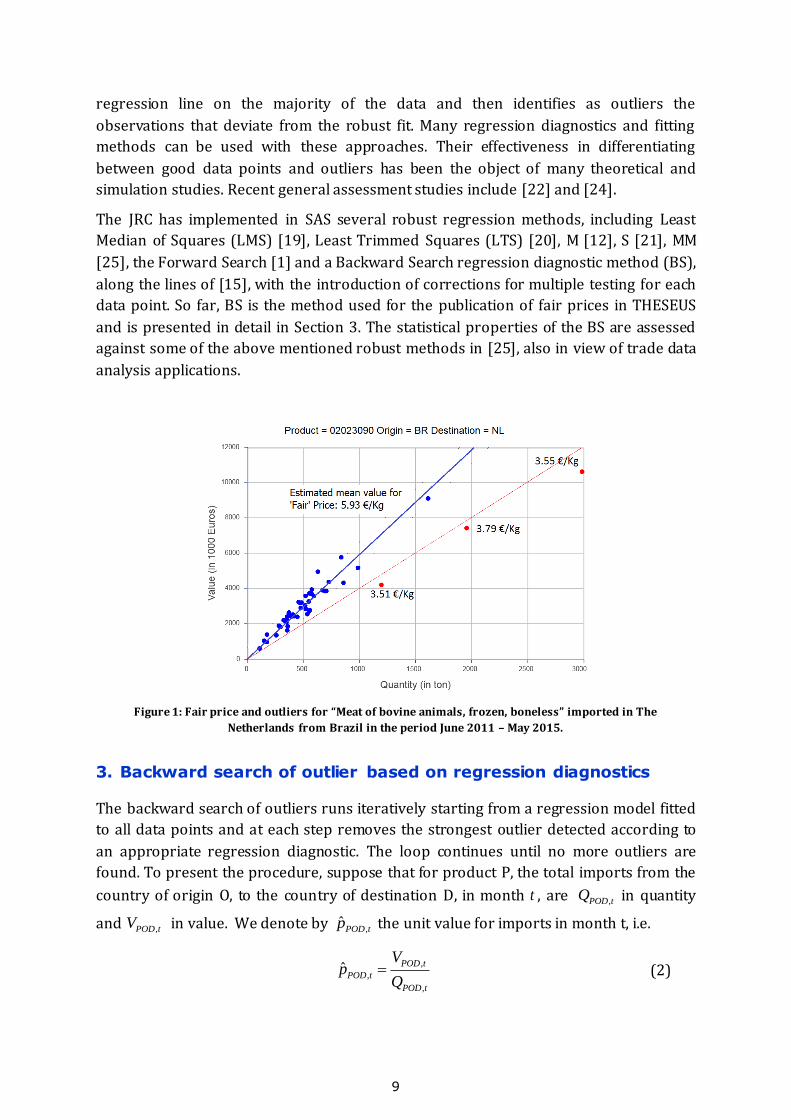
Figure 1 below illustrates the connection between the fair price estimation and the

outlier detection problem. A set of blue points lie rather well around a straight blue line

found using the popular least squares method, which goes back to Gauss and Legendre

(see for example [23], chapters 3 and 7). The three points in red deviate from the

regression line fit on the blue points and are considered to be outliers . The unit prices

associated with the outliers are approximately 3.6 €/Kg, while the blue line suggests a

price (the slope value) of about 6 €/Kg. The red line shows the potential effect of

including these outliers in the least squares fit: the line would be attracted by the

outliers and the price estimate (i.e. the line’s slope) would be considerably distorted.

In the statistical literature there are two general approaches to distinguish between the

subset of “good data points” and the outliers, which are extensively discussed, e.g., by

[18] and [3]. One uses regression diagnostic tools to suppress the outliers and fit the

remaining (supposedly good) data by least squares. The other, first fits a robust

9

regression line on the majority of the data and then identifies as outliers the

observations that deviate from the robust fit. Many regression diagnostics and fitting

methods can be used with these approaches. Their effectiveness in differentiating

between good data points and outliers has been the object of many theoretical and

simulation studies. Recent general assessment studies include [22] and [24].

The JRC has implemented in SAS several robust regression methods, including Least

Median of Squares (LMS) [19], Least Trimmed Squares (LTS) [20], M [12], S [21], MM

[25], the Forward Search [1] and a Backward Search regression diagnostic method (BS),

along the lines of [15], with the introduction of corrections for multiple testing for each

data point. So far, BS is the method used for the publication of fair prices in THESEUS

and is presented in detail in Section 3. The statistical properties of the BS are assessed

against some of the above mentioned robust methods in [25], also in view of trade data

analysis applications.

Figure 1: Fair price and outliers for “Meat of bovine animals, frozen, boneless” imported in The

Netherlands from Brazil in the period June 2011 – May 2015.

3. Backward search of outlier based on regression diagnostics

The backward search of outliers runs iteratively starting from a regression model fitted

to all data points and at each step removes the strongest outlier detected according to

an appropriate regression diagnostic. The loop continues until no more outliers are

found. To present the procedure, suppose that for product P, the total imports from the

country of origin O, to the country of destination D, in month t , are ,POD tQ in quantity

and ,POD tV in value. We denote by ,ˆ

POD tp the unit value for imports in month t, i.e.

,

,

,

ˆ POD t

POD t

POD t

Vp

Q (2)

10

An observation , ,,VPOD t POD tQ is considered as an outlier if it has a large studentized

deletion residual value for the linear model introduced in Section 2. The studentized

deletion residual is a traditional regression diagnostic presented in many textbooks (e.g.

[2], p. 23-24; [4], p. 18-21; [16]) that can be used to test the hypothesis of no outliers in

linear regression. In practice, at each step observations with significantly large

studentized deletion residual are removed. The significance level used for each outlier

test is the nominal significance level chosen by the user (e.g. 10%) corrected for the

total number of comparisons carried out (Bonferroni correction). If several

observations are significant, the observation to be removed is the one that makes the

largest difference in the regression results, as specified by its Cook distance (see again

[2], p. 24-25; [4], p. 15; [16]). More formally, the iterative algorithm follows this scheme:

1. Start with the full dataset, say 0( )S n where

0n indicates the initial number of

observations in the trade dataset POD. 2. Iterate the following steps:

a. Fit a regression line on ( )iS n .

b. Identify in set ( )iS n the observations for which the Studentized deletion

residual exceeds a critical value. Let ( )iSDR k be the subset of i ik n

observations. If ( )iSDR k is empty stop iterating and go to 3.

c. Computes the Cook distance for the observations in ( )iSDR k .

d. Remove from ( )iS n the observation with highest Cook distance, set

11 ii nn and go to 2a.

3. Fit a regression line on ( )tS n , the final subset found after t iteration steps.

4. Declare as outliers the observations in the original dataset 0( )S n for which the

Studentized deletion residual computed with respect to the fit on the final sub set

( )tS n exceeds a critical value.

5. Remove the outliers from the dataset 0( )S n and fit a (final) regression line on the *n good observations.

Note that the observations removed at the end of the loop (step 2) are only potential

outliers: some of them may be good observations having regression diagnostics

distorted at some step by the presence of other outliers. This is why in steps 4 and 5 we

reconsider each observation in the dataset and test their agreement to the stable model

estimate obtained at step 3.

The properties of iterative testing of the studentized residual, adopted by our backward

search outlier detection procedure, are studied in the statistical literature. It has strong

commonalities with the more general multistage procedure of Marasinghe [15] for

identifying up to k outliers in regression based on Studentized residuals. This

procedure was introduced as a simplification of an even more general method by

Gentleman and Wilk [11] for detecting the k most likely outlier subset based on

comparing the effects of deleting each possible subset of k observations in turn. These

general iterative testing approaches have drawbacks that make their use in applications

11

impractical: (i) one is the need to specify k in advance, and (ii) the substantial

computational effort involved even if k can be reasonably guessed in advance. In the

context of outlier detection, the use of Bonferroni inequalities to get an upper bound for

a critical value was studied, for example, by Lund [14], [12] and Prescott [16].

Appendix A recalls the mathematical details of the diagnostic regression statistics used

for the regression fit taken to intercept the origin, used in our context.

4. Estimation of fair prices and prediction of values for quantities

traded using outlier-free trade datasets

In the backward search for outliers the regression model fit changes as the method

iterates. At the end of the iterations, the estimated slope of the regression converges to

a stable and robust estimate of the unit value of imports of product P originating in

country O and imported into Member State D, let ˆPODp . In other words, the application of

the search procedure to a given POD dataset, results an outlier-free dataset on which an

estimate of the fair price of trade can be calculated with no influence from outliers that

could be initially present in the dataset . This fair price estimate is calculated as:

, ,

2

,

ˆPOD t POD t

tPOD

POD t

t

V Q

pQ

(3)

the index t taken over the outlier-free subset of *n observations in POD see, for

example, p. 458 of [5].

A useful measure of how well the estimated regression fits the *n observations is the so

called coefficient of determination R2, which for the model in section 2 is:

2

2, ,,

2

2 2 2

, , ,

ˆPOD t POD tPOD t

ttPOD

POD t POD t POD t

t t t

Q VV

RV Q V

(4)

Details on the R2 and a warning on pitfalls in using this statistic when models fit are not

linear with an intercept can be found in [13]. Appendix B gives a geometrical motivation

for the use of above R2 goodness of fit statistics for the regression model fitted to trade

data. In general, the R2 statistic varies between zero and one: higher values indicate that

the model fits the data better. If the observations on which the regression model is

estimated are perfectly aligned, i.e., the fit is perfect, then the R2 value is 1, There is no

formal threshold for R2 that can be used to decide if we can trust the regression model.

We suggest considering with particular caution combinations with a goodness of fit

smaller than 0.7.

A large goodness of fit provides evidence in support of the regression model and

strengthens our assurance with the fair price estimate. However, in general, except in

12

the case of perfect fit, it does not inform about the precision of the fair price estimated.

On the assumption that the proportional model of section 2 is valid for the monthly

trade retained as outlier-free, the standard error of the fair price is given by

*

2

,

1

ˆ PODPOD

n

POD i

i

SSE p

Q

(5)

where

*

22

, ,*1

1ˆ

1POD POD i POD POD i

i

n

S V p Qn

(6)

and *n is the number of outlier-free points in the dataset POD, see, for example, pages

459-460 of [5]. The (1 − 𝛼) confidence limits for the price 𝑝𝑃𝑂𝐷 is given by

* 1,1 /2ˆ ˆ

POD PODnp t SE p

(7)

where * ,1nt

is the upper 𝛼𝑡ℎ quantile for the t distribution with *n degrees of freedom.

Details on the interval estimation can be found in [4] and [16]. It is shown in appendix B

that the width (𝑊) of the confidence interval above can be seen to relate to the fair

price and the 𝑅2 as follows

*

2 2 2

* 21,1 /2

1 1ˆ 1

1PODn

POD

W t pn R

. (8)

The outlier-free dataset remaining after the exclusion of detected outliers can also be

used to predict the value traded for a new trade transaction. The (1 − 𝛼) confidence

limits for the value of a new trade transaction of quantity 𝑄𝑃𝑂𝐷,𝑎 is given by

* *

1/2

2

,

, 1,1 /22

,i

1

ˆ 1POD a

POD POD a PODn

POD

i

n

Qp Q t S

Q

. (9)

the index t taken over the outlier-free subset of observations in POD, see, for example, pp. 191-192 of [23].

13

5. Publication of results of fair prices in THESEUS

Figure 2 shows a small portion of the fair prices table, published in the THESEUS web

site, and calculated on imports into the EU, in the period December 2007-November

2010, as downloaded from COMEXT.

Figure 2: Example of fair prices from 14th COMEXT download

The rows in Figure 2 refer to lobsters imported into the EU. The selection of product

03062210 (Live lobsters “Homarus spp.”) has been done using the filtering feature of

the Product column heading, exemplified in Figure 3. This filtering feature is present in

all other fields.

Figure 3: Data in the table can be filtered out

Fair price tables in THESEUS are sorted by P, O, and D, but sorting in any other column

in the table is possible by dragging is the column heading to the area above. For

14

example, in Figure 2, the table is sorted by ascending fair price, so as to highlight

possible suspiciously low prices, at the top of the table.

The fair price table may contain columns that are of no interest to a user in his/her

particular work context. The user can select which columns to show from the drop-

down menu of the column headings, as shown in Figure 4.

Figure 4: User can sort the table by a field of interest and show/hide any field.

The “Outliers detected” column indicates the number of outliers removed by the BS

outlier detection procedure summarized in section 3 before the estimation of fair prices.

The column “Number of observations” in figure 2 gives the number of “clean” (outlier-

free) observations used for the fair price estimation. Intuitively, it is clear that we trust

more fair prices which are estimated using a larger number of , ,( , )POD t POD tQ V

observations.

As summarized in Section 2, the fair price estimate of a given POD is based on the linear

model through the origin assumed on the traded values and quantities. For this model,

in Section 4 we have given a measure of goodness of fit of the regression model, the so

called coefficient of determination R2. We said that this measure is a value between zero

and one and suggested considering with caution combinations with a goodness of fit

smaller than 0.7. As an example, note that in the THESEUS table of Figure 2 the R2

values are always high, above 0.9, except for the ID-NL combination, for which we have

R2 = 0.6.

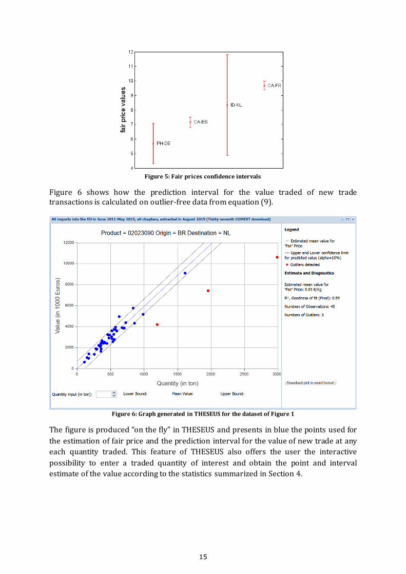
Figure 5 shows four price interval estimates for product 03062210 with the red ‘’ in

the middle of vertical lines representing each price interval. For imports from Canada

(CA) into Spain (ES) the interval is very tight and thus the fair price estimate is very

precise. The opposite situation is for ID-NL, where the price estimate can be at any place

in such a wide interval. The wide interval of ID-NL reflects a low R2 = 0.6 value, but not

the number of observations that is 35 (the maximum is 36 for this COMEXT run).

15

Figure 5: Fair prices confidence intervals

Figure 6 shows how the prediction interval for the value traded of new trade transactions is calculated on outlier-free data from equation (9).

Figure 6: Graph generated in THESEUS for the dataset of Figure 1

The figure is produced “on the fly” in THESEUS and presents in blue the points used for

the estimation of fair price and the prediction interval for the value of new trade at any

each quantity traded. This feature of THESEUS also offers the user the interactive

possibility to enter a traded quantity of interest and obtain the point and interval

estimate of the value according to the statistics summarized in Section 4.

16

6. References

[1] Arsenis, S. and Perrotta, D. (2010). Statistical Detection of Price outliers with a View

to Trade Based Money Laundering. Technical Report JRC 62691. Limited

distribution.

[2] Atkinson A. and M. Riani (2000). Robust Diagnostic Regression Analysis, Springer-

Verlag, NewYork.

[3] Barnett, V. & Lewis, T. (1984): Outliers in Statistical Data, 2nd ed., John Wiley &

Sons.

[4] Belsley, D. A., Kuh, E., and Welsch, R. E. (1980), Regression Diagnostics: Identifying

Influential Data and Sources of Coninearity, New York: Wiley.

[5] Box, G., Hunter, W.G. and J. S. Hunter (1978). Statistics for Experimenters, Wiley

New York.

[6] Cook, R. D., S. Weisberg (1982). Residuals and influence in regression. Chapman

and Hall. ISBN 041224280X, out of print, available on

http://www.stat.umn.edu/rir/

[7] Cook, R. D. (1977). Detection of influential observations in linear regression,

Technometrics, 19.

[8] Chatterjee, S. and Hadi, A. S (1986). Influential observations, high leverage points,

and outliers in linear regression, in: Statistical Science 1, pp. 379-416.

[9] Draper, N.R. and Smith, H. (1998). Applied Regression Analysis – Third Edition.

Wiley & Sons.

[10] Financial Action Task Force (2006). Trade Based Money Laundering, June 23,

2006, available at www.fatf-gafi.org.

[11] Gentleman, J. F., and Wilk, M. B. (1975), Detecting Outliers II: Supplementing the

Direct Analysis of Residuals. Biometrics, 31, 387-410.

[12] Huber, P.J. (1973), Robust regression: Asymptotics, conjectures and Montecarlo.

Annals of Statistics 1, 799-821.

[13] Kvalseth, T.O. (1985). Cautionary Note about 𝑅2. The American Statistician, 39,

279-285.

[14] Lund, R. E. (1975), Tables for an Approximate Test for Outliers in Linear Models.

Technometrics, 17, 473-476.

[15] Marasinghe, M. G. (1985), A Multistage Procedure for Detecting Several Outliers in

Linear Regression. Technometrics, 27, 395-399.

[16] Prescott, P. (1975). An Approximate Test for Outliers in Linear Models.

Technometrics, 17, 129-132.

[17] Rosenow, S. and O'Shea, B.J. (2010). A Handbook on the WTO Customs Valuation

Agreement.

[18] Rousseeuw, P.J. and Leroy, A.M. (1987). Robust Regression and Outlier Detection.

Wiley-Interscience, New York (Series in Applied Probability and Statistics).

[19] Rousseeuw, P.J., 1984. Least median of squares regression. Journal of the

American Statistical Association 79, 871–880.

17

[20] Rousseeuw, P.J., Van Driessen, K., 2006. Computing LTS regression for large data

sets. Data Mining and Knowledge Discovery 12, 29–45.

[21] Rousseeuw, P.J. and Yohai, V. (1984), Robust Regression by Means of S estimators.

in Robust and Nonlinear Time Series Analysis, edited by J. Franke, W. Härdle, and

R.D. Martin, Lecture Notes in Statistics 26, Springer Verlag, New York, 256-274.

[22] Salini S., Cerioli A., Laurini F., Riani M. (2015). Reliable robust regression

diagnostics. International Statistical review. To appear, available on-line: DOI:

10.1111/insr.12103.

[23] Seber, G.A.F. (1977). Linear Regression Analysis, John Wiley & Sons, New York.

[24] Torti F., Perrotta D., Atkinson A.C., Riani M. (2012). Benchmark Testing of

Algorithms for Very Robust Regression: FS, LMS and LTS. Computational Statistics

and Data Analysis, vol. 56, p. 2501-2512.

[25] Torti F. (2011). Advances in the Forward Search: Methodological and Applied

contributions, Best PhD Theses in Statistics and Applications: Statistics, CLEUP,

ISBN: 978-88-6129-719-7.

[26] Yohai V.J. (1987), High Breakdown Point and High Efficiency Robust Estimates for

Regression. Annals of Statistics, 15, 642-656.

[27] World Trade Organization (1994): WTO legal texts; General Agreement on Tariffs

and Trade 1994. Available at www.wto.org.

18

Appendix A: Regression Diagnostics

This section recalls the key regression diagnostics for a model fit without intercept

y x , where the regression slope is estimated by minimizing the sum of

squared residuals on n observations ( , )i ix y and is given by

2

ˆi i

i

i

i

x y

x

(10)

The regression analysis presented is valid under some common assumptions about the

observation errors : they are independent, have zero mean, constant variance 2 and

follow a normal distribution.

If an observation is an outlier we may want to remove it and refit the regression model,

especially if its removal makes a large difference in the regression results, i.e. if the

outlier is also influential. Following this idea, one may start from a fit to all the data and

iteratively adapt the model by removing observations on the basis of two statistics: the

studentised deletion residual, which indicates potential outliers, and the Cook distance,

which indicates influential observations. In general, it is not obvious to decide how

many and which observations should be removed at a given step. To check all possible

combinations is computationally demanding and the intermediate results may be

difficult to interpret, as the deletion of some influential observations may change

completely the statistics associated to other observations1. For this reason it is

customary to use deletion schemes that remove one observation at a time and monitor

how the regression model changes as the method proceeds, expecting to converge to a

subset of observations without outliers. The scheme presented in Section 3 removes the

most influential outlier, i.e. the observation of maximum Cook's distance among those

with studentised residual above its critical value.

The studentised residual

An outlier is an observation with large (in absolute value) residual. Several authors

have recommended the use of a residual that is standardized without considering that

observation, or RSTUDENT. The diagnostic is also called deletion residual2. If ˆi i ir y y

is the residual of an observation i , then the corresponding RSTUDENT is

1 This makes the approach potentially subject to masking or swamping effects: Barnett and Lewis define masking as "the tendency for the presence of extreme observations not declared as outliers to mask the discordancy of more extreme observations under investigation as outliers" ([3], p. 114). Likewise, the so called swamping effect concerns outliers that can influence the regression parameters at a point that one or more genuine observations appear as outliers.

2 In the literature there are other terms to indicate this form of standardised residual. Cook and Weisberg [6] use “externally studentized residual” in contrast to “internally studentized residual” when the context refer to both forms

of standardisations, with the current observation deleted or not. The terms “deletion residual” or “jackknife residual” are preferred by Atkinson and Riani ([2], p. 23-24). RSTUDENT is used by Belsley, Kuh, and Welsch ([4] p. 18-21).

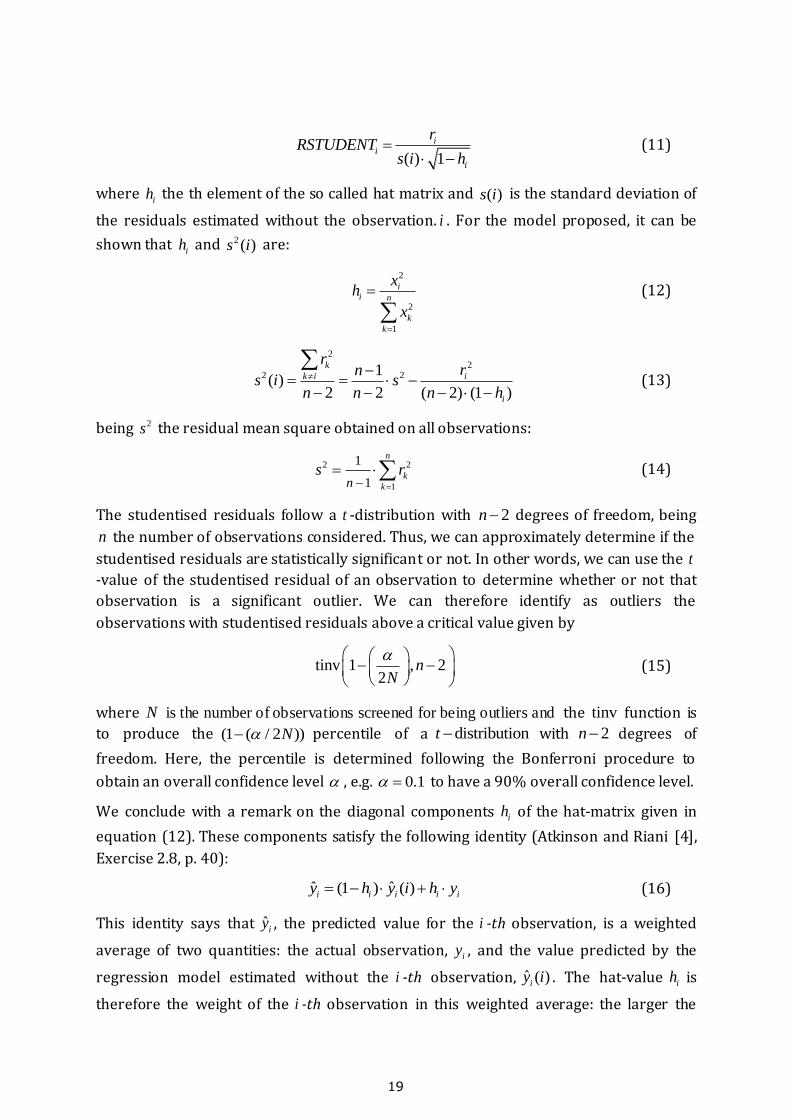
19

( ) 1

ii

i

rRSTUDENT

s i h

(11)

where ih the th element of the so called hat matrix and ( )s i is the standard deviation of

the residuals estimated without the observation. i . For the model proposed, it can be

shown that ih and 2 ( )s i are:

2

2

1

ii n

k

k

xh

x

(12)

2

22 21( )

2 2 ( 2) (1 )

k

k i i

i

rrn

s i sn n n h

(13)

being 2s the residual mean square obtained on all observations:

2 2

1

1

1

n

k

kns r

(14)

The studentised residuals follow a t -distribution with 2n degrees of freedom, being

n the number of observations considered. Thus, we can approximately determine if the

studentised residuals are statistically significant or not. In other words, we can use the t

-value of the studentised residual of an observation to determine whether or not that

observation is a significant outlier. We can therefore identify as outliers the

observations with studentised residuals above a critical value given by

tinv 1 , 22

nN

(15)

where N is the number of observations screened for being outliers and the tinv function is

to produce the (1 ( / 2 ))N percentile of a distributiont with 2n degrees of

freedom. Here, the percentile is determined following the Bonferroni procedure to

obtain an overall confidence level , e.g. 0.1 to have a 90% overall confidence level.

We conclude with a remark on the diagonal components ih of the hat-matrix given in

equation (12). These components satisfy the following identity (Atkinson and Riani [4],

Exercise 2.8, p. 40):

ˆ ˆ(1 ) ( )i i i i iy h y i h y (16)

This identity says that ˆiy , the predicted value for the i -th observation, is a weighted

average of two quantities: the actual observation, iy , and the value predicted by the

regression model estimated without the i -th observation, ˆ ( )iy i . The hat-value ih is

therefore the weight of the i -th observation in this weighted average: the larger the

20

weight, the more strongly the i -th observation will determine the prediction ˆiy . An

observation with an extreme value on the independent variable and, therefore, with big

hat-value, is called a high leverage point.

Cook’s distance

An observation is said to be influential if removing the observation changes

substantially the estimate of the regression coefficients. The Cook distance (Cook [4],

[7]), associated with an observation i , is a standardized distance measure between the

regression slope estimates and ( )i obtained with and without that observation. It

can be derived as follows. For the proposed model the impact on the slope of deleting

observation i is measured by (see Atkinson and Riani [2], p. 22-25, or Belsley, Kuh and

Welsch [4], p. 13):

2

( ) ii

j

j i

xi r

x

(17)

The denominator 2

j

j i

x

can be expressed as a function of the hat-value ih as follows,

2 2

22 2 2

2 2 21

1 1 1

1 1 1

j jnj i j ii

j j i i in n nj i j

j j j

j j j

x xx

x x x h h

x x x

giving:

2 2

1

(1 )n n

j i j

j i j

x h x

(18)

Substitution of the right-hand equation of (18) into (17) gives the desired distance

between the two slope estimates:

2

1

( )

(1 )

iin

i j

j

xi r

h x

(19)

Now, using (19), we can also measure the distance between the model predictions

obtained with and without observation i :

2

2

1

ˆ ˆ ( ) ( )(1 )

(1 )

i ii i i i in

ii j

j

x hy y i x i r r

hh x

(20)

21

For scaling purposes we can divide the distance ˆ ˆ ( )i iy y i by the standard deviation of

the prediction ˆiy , i.e. by3

2

1

ii

n

j

j

xh

x

(21)

where is the standard deviation of the observation errors. Therefore, equation (20)

becomes:

ˆ ˆ ( )

(1 )(1 )

ii i ii i

ii i i

hy y i hr r

hh h h

(22)

When is estimated by ( )s i (given in equation (13)) the right-hand side of is called by

Belsley, Kuh and Welsch [4] (p. 15) DFFITS (DiFference in FIT Standardised). If we take

the square of the above expression and estimate with the mean square error s

(given in equation (14)) we obtain the so called Cook’s distance:

2

2

2 2 2

ˆ ˆ ( )

(1 )

i i ii i

i i

y y i hD r

s h s h

(23)

This distance can be also expressed, like Cook did, in terms of ( )i rather than in

terms of the square of ˆ ˆ ( )i iy y i : it is sufficient to replace ih in the right term of the

above equation for iD with the expression given in equation (12), and use (19) to

obtain:

2 2

1

2

( )n

j

j

i

i x

Ds

(24)

Cook [4], [7] suggests that, in the general case of a regression model with p regressors,

the magnitude of this distance can be assessed by comparing iD to the probability

points of the ( , , )F p n p distribution. In this case iD becomes:

2

2 2(1 )

i ii

i

h rD

s h p

(25)

Among the cut-off values which have been proposed on that basis to identify influential

observations we mention 4/( 1)n p (Chatterjee and Hadi, [8]) and 2 /p n (Belsley,

Kuh and Welsch, [4]).

3 It seems more natural to divide ˆ ˆ ( )i iy y i by its own standard deviation: here we follow Cook’s choice.

22

Appendix B: The goodness of fit statistic for the proportional

regression model

The regression model between two variables without intercept -- also called the

proportional model -- can be written in vector notation as

Y X (26)

where and are the n dimensional vectors of response and predictor variables and

is the parameter to be estimated, or

1 1 1

... ... ...

n n n

y x

y x

(27)

As already mentioned in Section 4 and Appendix A, the least square estimate of is

known to be 2

1 1

ˆn n

i i i

i i

x y x

, where the variance of the estimated parameter is

2

2

1

ˆn

i

i

Var

x

(28)

and the unbiased estimate of 2 is

2

2

1

1 ˆ1

n

i i

i

S y xn

(29)

For the proportional regression model, we have that

2

2 2 2

1 1 1

ˆ ˆn n n

i i i i

i i i

y y x x

(30)

which can be thought of as the Pythagorean theorem in the n dimensional space of vectors and or, as the analysis of variance

2

Y 2

YY 2

Y

USS SSE SSM Uncorrected

Sum of Squares

Sum of Squares due to residuals

Sum of Squares due to regression (or due to model)

The geometric representation of the terms in the above equation is shown in Figure 7.

Y X

Y X

23

Figure 7: Geometric representation of the estimate and the analysis of variance terms

The Y vector is projected orthogonally on the space spanned by as the vector of

fitted values Y which equals X .

, the goodness of fit, is defined as the fraction of the sum of squares (SS) that can be explained by the regressor variable, i.e.:

2

2

2

ˆ

R

X

Y, (31)

and , in view of equation (26),

2

2

2

2 22 2

Ti i

i i

x y

Rx y

X Y

X Y (32)

and the following statements are equivalent:

1. 2 1R

2.

2

2 2

1 1 1

n n n

i i i i

i i i

x y x y

3. ˆ for all observations i

i

i

y

x

4. 2

1

ˆSSE 0n

i i

i

y x

and hold when there is perfect fit in the data.

X

2R

0

24

To relate the standard error of to 2R and , note that because of equations (27) and

(28) and the equation for ,

22 2

2 2 2

2 2 21 1 1

1 1 1

1 1 1 1ˆ ˆ ˆSE1 1

n n n

i i i in n ni i i

i i i

i i i

Sy x y x

n nx x x

(33)

The right hand side of which can be written as

2 22 2

2 2

1 1 1 1ˆ ˆ 11 1n n R

Y XX

(34)

because of equation (30). This is equation (8) given in section 4.

25

Appendix C: Acquisition of the data from COMEXT and their

maintenance.

This appendix describes the procedure adopted by the JRC for the download of the COMEXT data. The procedure is stable over time, to ensure the reproducibility of the fair price estimates published in the THESUS website.

COMEXT data are revised frequently, according to national practices, on the basis of updates and corrections that are communicated to ESTAT by the Member States nearly on a daily basis. ESTAT makes the revisions available at each monthly update and normally data become final after six to twelve months after the reference year. Exceptional revisions of older data are usually done once per year, around June. ESTAT makes the most recent data and different supplements for annual and historical data available through DVDs and a web-based bulk download facility4. The ESTAT bulk download contains the following items:

The datasets in tsv (tab separated values), dft and sdmx format, which are used to import

the data in our database.

Guidelines on how to automate the download of datasets.

A manual containing all detailed information on the bulk download facility.

The table of contents that includes the list of the datasets available.

The "dictionaries" of all the coding systems used in the datasets. In collaboration with OLAF, the JRC has started using COMEXT data to detect patterns of interest in complete datasets on imports into the EU. The data extracted from COMEXT, for purposes of communication of results obtained, are enumerated in the THESUS website of the JRC as “downloads”: the 38th is a recent one and is shown in the Figure 8 below, together with a selection of the set of fair prices based on this download.

Figure 8: The THESEUS fair prices for different "COMEXT downloads"

The publication date of the monthly bulk download of ESTAT is the fixed reference date of the fair prices in THESEUS. In Figure 8 the download reference date is reported as

4 The bulk download facility of ESTAT is accessible at the url: http://ec.europa.eu/eurostat/data/bulkdownload

26

“Last update” in the “Download (DLs)” panel on the left of the table, together with indication of the period covered by the import data used for the fair price estimation. Each period includes the latest 48 months of import data. Note that the data period ends three months before the reference date of the download. This choice has been made to ensure the use of relatively stable data in the production of stable price estimates, as the most recent data is typically subject to substantial revisions.

In order to guarantee the reproducibility of the fair price estimates, we keep the history of the monthly changes made by ESTAT of the downloaded data in a MySQL database and in backup files. The history of each record is preserved by two fields, “IdFrom” and “IdTo”, that identify the initial and final downloads where the record is valid. The table below contains the complete structure of the COMEXT data stored in the JRC database.

FIELD NAME FORMAT

PRODUCT char(8) PARTNER char(2)

DECLARANT char(2) PERIOD date

VALUE_1000EURO decimal(36,2) QUANTITY_TON decimal(36,2)

SUP_QUANTITY decimal(42,0)

IdFrom int(11) IdTo int(11)

Table 1: Fields of the COMEXT data stored in the JRC database

When a new download is released by ESTAT, we do the following operations:

a) We archive the backup file of the downloaded data; b) We add to our database the records of the new download that were not present in previous

downloads; c) We add to our database the records that were already present in previous download but

that have been revised by ESTAT. We can easily identify these records, because they have the same key (i.e. same PRODUCT, ORIGIN, DESTINATION and PERIOD) but different VALUE_1000EURO or QUANTITY_TON values.

The next table shows an example of a record revised in different downloads. The list of the different instances of the record is extracted with this simple SQL query:

SELECT *

FROM @tablename

WHERE `PRODUCT` = '81089050'

AND `PARTNER` = 'QY'

AND `DECLARANT` = 'DK'

AND `PERIOD` = '2014-02-01';

VALUE_1000EURO QUANTITY_TON SUP_QUANTITY IdFrom IdTo

166.23 12.90 24 24 293.71 20.70 25 25

149.87 11.90 0 26 26 132.76 10.80 27 27

156.07 12.00 28 29 139.89 11.00 0 30 30

149.49 11.50 0 31 31

147.90 11.40 0 32 33

27

135.90 10.70 0 34 34 136.78 10.80 0 36 36

135.92 10.80 0 37 37 137.34 10.80 0 38 38

139.34 10.90 0 39 39

Table 2: Result of a query to retrieve all instances of a record with same key in different downloads

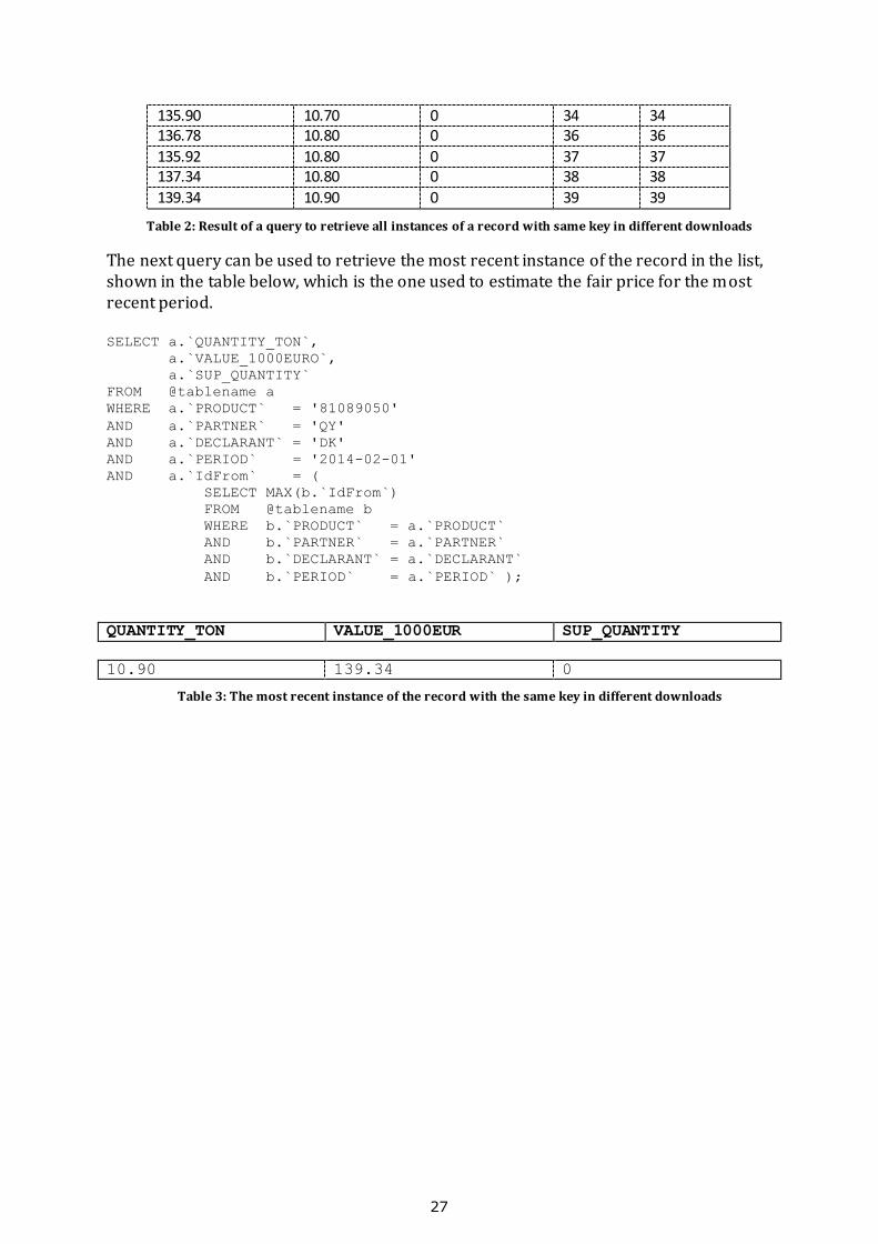
The next query can be used to retrieve the most recent instance of the record in the list, shown in the table below, which is the one used to estimate the fair price for the most recent period. SELECT a.`QUANTITY_TON`,

a.`VALUE_1000EURO`,

a.`SUP_QUANTITY` FROM @tablename a WHERE a.`PRODUCT` = '81089050'

AND a.`PARTNER` = 'QY'

AND a.`DECLARANT` = 'DK' AND a.`PERIOD` = '2014-02-01' AND a.`IdFrom` = ( SELECT MAX(b.`IdFrom`) FROM @tablename b WHERE b.`PRODUCT` = a.`PRODUCT` AND b.`PARTNER` = a.`PARTNER` AND b.`DECLARANT` = a.`DECLARANT` AND b.`PERIOD` = a.`PERIOD` );

QUANTITY_TON VALUE_1000EUR SUP_QUANTITY

10.90 139.34 0

Table 3: The most recent instance of the record with the same key in different downloads

How to obtain EU publications

O ur publications are available from EU Bookshop (http://bookshop.europa.eu),

where you can place an order with the sales agent of your choice.

The Publications O ffice has a worldwide network of sales agents.

You can obtain their contact details by sending a fax to (352) 29 29-42758.

Europe Direct is a service to help you find answers to your ques tions about the European Union

Free phone number (*): 00 800 6 7 8 9 10 11

(*) C ertain mobile telephone operators do not allow access to 00 800 numbers or these calls may be billed.

A great deal of additional information on the European Union is available on the Internet.

I t can be accessed through the Europa server http://europa.eu

2

doi:10.2788/3790

ISBN 978-92-79-54576-4

LB-N

A-2

7696-E

N-N

JRC Mission

As the Commission’s

in-house science service,

the Joint Research Centre’s

mission is to provide EU

policies with independent,

evidence-based scientific

and technical support

throughout the whole

policy cycle.

Working in close

cooperation with policy

Directorates-General,

the JRC addresses key

societal challenges while

stimulating innovation

through developing

new methods, tools

and standards, and sharing

its know-how with

the Member States,

the scientific community

and international partners.

Serving society Stimulating innovation Supporting legislation