THE EMPLOYMENT IMPACTS OF ECONOMY-WIDE
202
THE EMPLOYMENT IMPACTS OF ECONOMY-WIDE INVESTMENTS IN RENEWABLE ENERGY AND ENERGY EFFICIENCY A Dissertation Presented by HEIDI GARRETT-PELTIER Submitted to the Graduate School of the University of Massachusetts Amherst in partial fulfillment of the requirements for the degree of DOCTOR OF PHILOSOPHY September 2010 Economics
Transcript of THE EMPLOYMENT IMPACTS OF ECONOMY-WIDE

THE EMPLOYMENT IMPACTS OF ECONOMY-WIDE INVESTMENTS IN RENEWABLE ENERGY AND ENERGY EFFICIENCY
A Dissertation Presented
by
HEIDI GARRETT-PELTIER
Submitted to the Graduate School of the University of Massachusetts Amherst in partial fulfillment
of the requirements for the degree of
DOCTOR OF PHILOSOPHY
September 2010
Economics

© Copyright by Heidi Garrett-Peltier 2010
All Rights Reserved

THE EMPLOYMENT IMPACTS OF ECONOMY-WIDE INVESTMENTS IN RENEWABLE ENERGY AND ENERGY EFFICIENCY
A Dissertation Presented
by
HEIDI GARRETT-PELTIER
Approved as to style and content by: ____________________________________ Robert Pollin, Chair ____________________________________ Michael Ash, Member ____________________________________ James Heintz, Member ____________________________________ Stephanie Luce, Member
____________________________________ Gerald Epstein, Department Chair Economics

iv
ACKNOWLEDGEMENTS
I would like to extend my sincere appreciation to my committee for their
involvement and commitment in this process. I am grateful to my committee chair, Bob
Pollin, for his guidance, encouragement, mentoring, and kindness throughout the writing
of this dissertation. I thank each of my committee members for the unique role that each
played: James Heintz for his wisdom and patience as he helped me work through some of
the intricacies of input-output modeling; Michael Ash for his insistence that I relate my
work to the broader field of climate change and also for his technical advice; and
Stephanie Luce for her guidance as I developed, conducted, and evaluated the survey.
I am grateful to the Department of Economics and to the Political Economy
Research Institute for providing the funding, education, inspiration, and fertile
intellectual atmosphere that enabled me to complete this work. I thank the members of
the Environmental Working Group for their feedback at various points throughout this
process. I also thank my survey team for their persistence and hard work in making
phone calls and emailing hundreds of contacts.
Finally, I wish to thank my parents, Michele and Michael, and my wife, Graysen,
for their enduring love and support.

v
ABSTRACT
THE EMPLOYMENT IMPACTS OF ECONOMY-WIDE INVESTMENTS IN RENEWABLE ENERGY AND ENERGY EFFICIENCY
SEPTEMBER 2010
HEIDI GARRETT-PELTIER, B.A., UNIVERSITY OF CONNECTICUT STORRS
M.A., UNIVERSITY OF MASSACHUSETTS AMHERST
Ph.D., UNIVERSITY OF MASSACHUSETTS AMHERST
Directed by: Professor Robert Pollin
This dissertation examines the employment impacts of investments in renewable
energy and energy efficiency in the U.S. A broad expansion of the use of renewable
energy in place of carbon-based energy, in addition to investments in energy efficiency,
comprise a prominent strategy to slow or reverse the effects of anthropogenic climate
change.
This study first explores the literature on the employment impacts of these
investments. This literature to date consists mainly of input-output (I-O) studies or case
studies of renewable energy and energy efficiency (REEE). Researchers are constrained,
however, by their ability to use the I-O model to study REEE, since currently industrial
codes do not recognize this industry as such. I develop and present two methods to use
the I-O framework to overcome this constraint: the synthetic and integrated approaches.
In the former, I proxy the REEE industry by creating a vector of final demand based on
the industrial spending patterns of REEE firms as found in the secondary literature. In
the integrated approach, I collect primary data through a nationwide survey of REEE
firms and integrate these data into the existing I-O tables to explicitly identify the REEE

vi
industry and estimate the employment impacts resulting from both upstream and
downstream linkages with other industries.
The size of the REEE employment multiplier is sensitive to the choice of method,
and is higher using the synthetic approach than using the integrated approach. I find that
using both methods, the employment level per $1 million demand is approximately three
times greater for the REEE industry than for fossil fuel (FF) industries. This implies that
a shift to clean energy will result in positive net employment impacts. The positive
effects stem mainly from the higher labor intensity of REEE in relation to FF, as well as
from higher domestic content and lower average wages. The findings suggest that as we
transition away from a carbon-based energy system to more sustainable and low-carbon
energy sources, approximately three jobs will be created in clean energy sectors for each
job lost in the fossil fuel sector.

CONTENTS
Page
ACKNOWLEDGMENTS ................................................................................................. iv
ABSTRACT .........................................................................................................................v
LIST OF TABLES ............................................................................................................. xi
LIST OF FIGURES ......................................................................................................... xiii
LIST OF ABBREVIATIONS .......................................................................................... xiv
CHAPTER
1. INTRODUCTION ...................................................................................................1
Background on Climate Change, Renewable Energy and Energy Efficiency......................................................................4
The Threat of Climate Change .........................................................4
Current and Projected Energy Use .................................................12
Carbon Productivity .......................................................................16
2. LITERATURE REVIEW ......................................................................................21
Introduction ................................................................................................21
Estimating the Employment Impacts of Energy Policy .............................22
Overview of models .......................................................................22
Input-Output and Linear Models ...................................................26
Employment Created Directly through REEE Investment ...................................................29
Employment Created through Energy Savings ..................39
Non-Modeled Employment Analysis ............................................51
Case Studies .......................................................................51
Case Studies Combined with Secondary Data ...................54
Advantages and Disadvantages of Renewable Energy Case Studies ............................57
Discussion of Choice of Input-Output Model ............................................58
3. USING THE INPUT-OUTPUT MODEL TO STUDY RENEWABLE ENERGY AND ENERGY EFFICIENCY ................................................60
The Input-Output Model ............................................................................60
Background ....................................................................................60
Estimating Employment Multipliers Using the Input-Output Model ...........................................................65
Assumptions Embodied in the Input-Output Model ......................70
Creating “Synthetic” Industries in the I-O Model .....................................72
Background and Motivation ..........................................................72
Recent Applications .......................................................................75
Testing the Validity of the Synthetic Industry Approach ..............78
4. SURVEY OF RENEWABLE ENERGY AND ENERGY EFFICIENCY FIRMS ..............................................................81
Background and Motivation for Survey ....................................................81
Selecting Sample ........................................................................................82
Sample Size ....................................................................................82
Assembling Population List ...........................................................83
Random Sample Selection .............................................................85
Enlarging Sample ...........................................................................85
Questionnaire Design .................................................................................86
Questionnaire Content ...................................................................86
Questionnaire Form .......................................................................87
Testing Questionnaire ....................................................................88
Responses ...................................................................................................88
5. INTEGRATING SURVEY DATA .......................................................................91
Converting data to consistent base year .....................................................92
Adjusting for Inflation ...................................................................92
Adjusting for Growth .....................................................................92
Scaling Survey Responses to National Industry Level ..............................94
Methodology for Integrating Results .......................................................101

Incorporating a Single REEE Industry ........................................101
Incorporating 3 Distinct REEE Industries ...................................106
6. RESULTS AND DISCUSSION ..........................................................................109
Results ......................................................................................................109
Survey Integration Results ...........................................................109
REEE Industry .................................................................109
Three Distinct REEE Industries .......................................111
Synthetic Industry Results ...........................................................112
Industries and Weights .....................................................112
Using Synthetic Industry Approach with Survey Data ................113
Robustness Tests ..........................................................................115
Survey Integration Robustness Tests ...............................115
Synthetic Industry Specification Tests.............................116
Discussion ................................................................................................119
Comparison of Results from Alternative Methods ......................119
Comparing Results to Other Studies ............................................120
Reasons for Differences between Methods ..................................121
Differences in Output and Employment Multipliers .......122
Differences in Employment/Output Ratios ......................124
Differences in Final Demand ...........................................127 Inherent Methodological Differences ..............................129
Which Estimation Method Is More Accurate or Appropriate? ................................................................................130
Policy Implications of Alternative Approaches ...........................132
7. CONCLUSION ....................................................................................................134
Chapter Summary ....................................................................................134
Contributions of this Dissertation ............................................................137
Policy Implications ..................................................................................138 Directions for Further Research ...............................................................139

APPENDIX: SURVEY QUESTIONNAIRE .................................................................178
BIBLIOGRAPHY ............................................................................................................184

xi
LIST OF TABLES
Table Page
1. U.S. Energy Consumption by Energy Source, 2004 - 2008 .....................................142
2. Renewable Energy Power Generation – Level and Growth, 2007-2035 ..................143
3. Selected Employment Multipliers from BEA Input-Output Tables .........................144
4. Specification Test for Synthetic Industry, Using Wind Industry as Example ..........145
5. Sample Size and Sampling Error for the 95 percent Confidence Interval ................146
6. Summary Statistics of Survey Responses .................................................................147
7. Survey Responses Grouped into 3 Distinct Categories ............................................148
8. 2005-2007 Growth by REEE Industry Group ..........................................................149
9. Employment/Output Ratios for 66-industry Employment Requirements Matrix ...................................................................................................................150
10. Employment/Output Ratios from REEE Survey Data .............................................152
11. Employment Multipliers in Original and Expanded I-O Tables ..............................153
12. Total Employment Multipliers for Original, 65x65, and 68x68 I-O Tables ............156
13. Composition of Synthetic REEE Industries .............................................................159
14. Employment Multipliers of Various REEE Industries Using Synthetic Approach ..............................................................................................................160
15. Composition of Industries Using Hybrid Approach ................................................161
16. Employment Multipliers Using Hybrid Approach ..................................................163
17. Specification Tests for the Green Program ..............................................................164
18. Specification Tests for the REEE Industry ..............................................................165

xii
19. Employment Multipliers from Integrated, Synthetic, and Hybrid Approaches .......166
20. Comparison with REEE multipliers from previous studies .....................................167
21. Output Multipliers from Leontief Inverse Matrices.................................................168
22. Source of Variation in REEE Employment Multipliers ..........................................171
23. REEE Employment Multipliers Using Industry Average E/O Ratio.......................172
24. Comparison of Sources of Variation in Employment Multipliers ...........................173
25. Differences in Composition of Final Demand for REEE and Green Program ........174
26. Comparison of Fossil Fuel and REEE Employment Multipliers .............................175

xiii
LIST OF FIGURES
Figure Page
1. Employment impacts of alternative energy sources, Table 4 from (Pollin, Heintz, & Garrett-Peltier, 2009).....................................176
2. Energy Industries and Weights, from (Pollin, Heintz, & Garrett-Peltier, 2009) ......177

xiv
LIST OF ABBREVIATIONS
ACEEE American Council for an Energy-Efficient Economy
AEO Annual Energy Outlook
BEA Bureau of Economic Analysis
BLS Bureau of Labor Statistics
BTU British Thermal Unit
CCS Carbon Capture and Sequestration
CCSP Climate Change Science Program
CGE Computable General Equilibrium
CO2 Carbon dioxide
CO2e Carbon-equivalent emissions
DOE Department of Energy
EIA Energy Information Administration
EWEA European Wind Energy Association
FTE Full-time Equivalent
GDP Gross Domestic Product
GHG Greenhouse Gas
Gt Gigaton
IAM Integrated Assessment Model
IEA International Energy Agency
I-O Input-Output
IPCC Intergovernmental Panel on Climate Change
kWh Kilowatt hours
LIFT Longterm Interindustry Forecasting Tool

xv
MW Megawatt
Mwa Average Megawatt
NAICS North American Industrial Classification System
NASA National Aeronautics and Space Administration
PERI Political Economy Research Institute
PPI Producer Price Index
ppmv parts per million volume
pv Photovoltaic
REEE Renewable Energy and Energy Efficiency
REPP Renewable Energy and Policy Project
RPS Renewable Portfolio Standard
SAM Social Accounting Matrix
TPG The Perryman Group

1
CHAPTER 1
INTRODUCTION
The threat of climate change has recently become a reality in the public mind. An
abundance of scientific evidence – from the Stern Review to various reports by the
Intergovernmental Panel on Climate Change – has shown that carbon emissions threaten
our ecosystem and may cause irreversible and devastating impacts to the planet and our
way of life (Stern, 2007), (Schneider, et al., 2007). In the face of such evidence, the need
for an energy transition has become clear. To reduce carbon emissions, it is imperative to
reduce our consumption of freely-emitting fossil fuels, the primary contributor of these
emissions. This can happen through three channels – replacing fossil fuel consumption
with energy consumption from low-carbon energy sources such as wind, solar, biomass,
and nuclear power; capturing the carbon that is emitted from the burning of fossil fuels
and storing it (“carbon capture and storage”, or CCS)1; and increasing energy efficiency
and conservation so that we reduce our overall level of demand for primary energy.
Until recently, this pro-environment transition was touted as bad for the economy.
Now, however, the tide seems to be turning, and “green growth” is increasingly
advocated as a way to create more jobs while increasing environmental sustainability. A
report issued by McKinsey & Company, a worldwide consulting firm who in recent years
1 CCS is not yet a commercially available technology, and assumptions on the timing and cost of CCS technology vary widely. In this dissertation, I will not explore investment or employment in this fledgling technology. However, many climate models consider CCS to be an important strategy for reduced emissions. See, for example, (Clarke et al, 2007), (Paltsev et al, 2009), and (Fawcett et al, 2009).

2
has become a leader in climate change policy analysis, refers to this as the “carbon
productivity challenge” (McKinsey Global Institute, 2008). "Carbon productivity" is the
amount of GDP produced per unit of carbon equivalent emissions (CO2e). It is a useful
concept for considering climate change mitigation in tandem with economic growth. As
the authors point out, there is "agreement approaching consensus that any successful
program of action on climate change must support two objectives - stabilizing
atmospheric greenhouse gases and maintaining economic growth" (p 7) and that to obtain
both objectives we need to drastically increase our carbon productivity.
In response to this rising public consciousness in support of green growth, there is
a growing body of literature examining the economic effects of climate change
mitigation, to which we will turn below. While many studies focus on the global impacts
on GDP of action or inaction, other studies take a more targeted approach and examine
the effects of national and regional strategies. Within this, we find studies addressing the
employment impacts of climate change action, including investments in the renewable
energy and energy efficiency (REEE) industry. If we shift from a fossil-fuel-based
economy to one in which we use energy more efficiently and generate more power from
renewable sources, what are the economic impacts? Which industries will gain from this
energy transition, and which will lose? The obvious answer is that coal, oil and natural
gas will lose while solar, wind, biomass, and other renewables gain. However, the
picture is more complicated as each of these industries buys and sells goods and services
from other industries in the economy. Thus we need to examine inter-industry
relationships and employment patterns across industries in order to determine economy-
wide employment impacts of a clean-energy transition.

3
In this dissertation, I will contribute to the literature on the employment impacts
of investments in renewable energy and energy efficiency. I will explore the current state
of this literature, then expand the methodology that has been used thus far and
incorporate new data on REEE firms in the U.S. that I collected through an extensive
survey process. I will present the results of various estimation methods using primary
and secondary data.
The remainder of this dissertation is organized as follows. In Chapter 2 I first
review the growing literature on the employment impacts of REEE investments. We will
see that to date, researchers have been constrained in their ability to analyze the REEE
industry due to data limitations. Nonetheless, a number of studies have been conducted
using input-output modeling, case studies, and interviews, to gauge the employment
effects of investments in REEE. Across the board, these studies have found that a shift
from fossil fuels to REEE will engender positive employment effects. In Chapter 3 I will
then discuss the input-output model, commonly used to estimate REEE employment
impacts, and will create ‘synthetic industries’ which allow us to use the existing input-
output tables in the absence of REEE-specific data. To overcome this limitation with
currently available public data, I conducted an extensive survey of REEE firms
throughout the U.S. I discuss the survey process and results in Chapter 4, and then in
Chapter 5 present the methodology for integrating the survey results into existing input-
output tables. This methodology is an innovation in the REEE literature and allows us to
identify the REEE industry within the I-O tables and to estimate REEE employment in a
manner consistent with employment in other industries. In Chapter 6 I then present the
employment estimation results of these alternative methods. I also perform robustness

4
tests and compare my results to each other and to estimates published by other
researchers. We will see that by all measures, investments in REEE will generate
positive employment impacts, even after we consider job losses in fossil fuels. Finally
Chapter 7 contains concluding remarks.
In the remainder of this introduction I offer some background on the climate
change debate as well as current and projected levels of renewable energy, energy
efficiency, and global emissions.
Background on Climate Change, Renewable Energy and Energy Efficiency
The Threat of Climate Change
There is now an abundance of scientific evidence that we are currently
experiencing anthropogenic (human-caused) climate change, and that carbon emissions
are primarily to blame for global warming and other extreme weather events. The
Environmental Protection Agency writes that:
If greenhouse gases continue to increase, climate models predict that the average temperature at the Earth's surface could increase from 3.2 to 7.2ºF above 1990 levels by the end of this century. Scientists are certain that human activities are changing the composition of the atmosphere, and that increasing the concentration of greenhouse gases will change the planet's climate. But they are not sure by how much it will change, at what rate it will change, or what the exact effects will be.2
The Intergovernmental Panel on Climate Change, convened by the United
Nations Environment Programme and the World Meteorological Organization, is a body
of thousands of scientists worldwide who have reviewed hundreds of scientific, technical,
2 EPA, accessed 4/8/08 at http://www.epa.gov/climatechange/basicinfo.html

5
and socio-economic studies of climate change. The results of the most recent completed
assessment by the IPCC, the Fourth Assessment, were published in 2007. IPCC scientists
found that "warming of the climate system is unequivocal" and that "Global greenhouse
gas emissions due to human activities have grown since pre-industrial times, with an
increase of 70% between 1970 and 2004" (IPCC, 2007, p. 30-36). Carbon dioxide is the
most important source of anthropogenic greenhouse gas emissions, and its annual
emissions grew by about 80% between 1970 and 2004, primarily from the use of fossil
fuels (p. 36). While global energy intensity fell over the period, both population and
income grew globally, resulting in overall growth in greenhouse gas (GHG)
emissions. Global atmospheric concentration of CO2, a measure commonly used in the
literature to gauge the level and change of carbon dioxide, increased from a pre-industrial
value of about 280 parts per million volume to 379ppmv in 2005 (IPCC, 2007, p. 37).”
While the precise implications for human welfare cannot be determined, various
models predict a range of probable outcomes that increase in severity as the Earth’s
surface increases in temperature. For example, a team of scientists who form Working
Group II of the IPCC have cataloged temperature-specific outcomes for humans as well
as the rest of the eco-system (Parry, et al., 2007). They show that for global temperature
rises of 3-5 degrees, risks (that are unevenly distributed) include such things as water
shortages, coastal flooding, increased risk of malaria in some areas, reductions in crop
yields, more extreme weather events, increased extinction of certain species, increased
conflicts resulting from food and water shortages as well as changing migration patterns,
and more severe market losses in low-altitude areas. The U.S. National Aeronautics and
Space Administration (NASA) writes that “global climate change has already had

6
observable effects on the environment” including glacial melting, changing plant and
animal ranges, and trees flowering sooner, and that “the potential future effects of global
climate change include more frequent wildfires, longer periods of drought in some
regions and an increase in the number, duration and intensity of tropical storms.”3
Economists, scientists and others have suggested that in order to prevent truly
devastating consequences, we must act not only to halt any increase in our carbon
emissions but also to reverse the rising trend and to lower emissions to below their 1990
levels. The policy recommendations for the speed and magnitude of the necessary
changes vary among studies. On one end of the spectrum, the recommendations of
Nicholas Stern are for “strong, early action” to stop and reverse any increase in emissions
(Stern, 2007). Other the other end of the spectrum is William Nordhaus, who advocates a
gradual policy ramp as the most economically efficient response to climate change, with
slow and small steps now, gradually increasing in scope over the course of the century
(Nordhaus, 2008). James Hansen of NASA as well as Rajendra Pachauri (head of the
IPCC) support the Stern recommendations, which are to keep atmospheric concentrations
of carbon dioxide to 385ppm or less, even to lower them to 350ppm (which would
involve ‘negative emissions’ through strategies such as reforestation). At the heart of the
issue of whether to act immediately or to follow a gradual ‘policy ramp’ are two factors:
the discount rate and the level of climate sensitivity4. Both factors are chosen by the
modeler, rather than being results of the model, and therefore changing an assumption 3 http://climate.nasa.gov/effects/ accessed 4/20/2010
4 The discount rate includes both the pure rate of time preference as well as a rate of return on capital. Climate sensitivity refers to the increase in temperature that results from a doubling of carbon dioxide emissions.

7
about either factor will change the policy prescription. A low discount rate combined
with a higher level of climate sensitivity (greater temperature increases, which in turn
cause greater damages) will lead to recommendations for immediate action, as promoted
by Stern. Nordhaus, on the other hand, uses a higher discount rate and lower level of
climate sensitivity, resulting in the call for more gradual action. Frank Ackerman and
others have shown that by using the Nordhaus model (DICE-2007) and changing these
assumptions, even this model recommends immediate and drastic action (Ackerman, et
al., 2008). Of course, actions and outcomes decades into the future are uncertain and
unknowable, and even the best model cannot precisely predict economic or ecological
outcomes in 2050 or 2100. Nordhaus himself points out that IAMs (Integrated
Assessment Models) cannot be used to predict actual outcomes, but only to estimate the
effects of various scenarios or policy choices. "The purpose of integrated assessment
models is not to provide definitive answers to these questions [of the trajectories of
emissions, growth, or carbon taxes], for no definitive answers are possible, given the
inherent uncertainties about many of the relationships. Rather, these models strive to
make sure that the answers at least are internally consistent and at best provide a state-of-
the-art description of the impacts of different forces and policies (Nordhaus, 2008, p. 9)."
Many studies model reference scenarios and alternative stabilization scenarios,
which estimate the effects of targeting certain atmospheric concentrations of CO2. For
instance, the U.S. Climate Change Science Program and the Subcommittee on Global
Change Research engaged three leading climate models (IAMs) to explore a reference
scenario and four alternative stabilization scenarios based on varying levels of radiative
forcing (warming) and corresponding atmospheric concentrations of greenhouse gases by

8
2100. The models used are the Integrated Global Systems Model (IGSM) by MIT, the
MERGE model developed jointly by Stanford University and the Electric Power
Research Institute, and the MiniCAM Model of the Joint Global Change Research
Institute, a partnership between the Pacific Northwest National Laboratory and the
University of Maryland.
In the reference scenarios, radiative forcing in 2100 is three to four times as high
as pre-industrial levels, and primary energy consumption increases three to four times
2000 levels as economic growth outpaces improvements in energy efficiency. Global
CO2 emissions in the reference scenario double and nearly triple between 2000 and 2100,
reaching 700 to 900 ppm, up from 365 ppm in 1998. Thus the reference scenario results
for carbon emissions are well above the levels recommended by Stern, IPCC, and others.
In the various stabilization scenarios of the CCSP report, which correspond
roughly to 450, 550, 650, and 750 ppm, CO2 emissions peak and decline in the 21st
century, with the timing dependent upon the level of stringency. The 450 ppm
concentration necessitates an immediate decline in CO2 emissions. In all scenarios, the
greenhouse gas reductions require a transformation of the global energy system,
including reductions in the demand for energy and changes in the mix of technologies
and fuels.
Whether we follow the drastic measures advocated by Stern and others, the
gradual policy ramp suggested by Nordhaus, or a pathway in between, virtually all
studies of climate change show that emissions reductions in the next century are
necessary. This can be done mainly by reducing our use of carbon-based fuel sources,

9
which we can achieve by reducing our levels of energy demand (through efficiency and
conservation) and by replacing our carbon-based energy use with low-carbon or carbon-
free sources. As mentioned above, some studies also advocate the use of carbon capture
and storage (CCS) as a way to reduce our carbon emissions. While this may be a viable
solution in the medium term, CCS is not yet a commercially available technology. In this
dissertation I will restrict my attention to energy efficiency and renewable energy –
mitigation solutions that are already available and in practice.
The transition to a clean-energy economy will entail both costs and benefits.
Much of the climate change literature focuses on the costs of adaptation and mitigation,
rather than the benefits of doing so (or, in other words, the benefits are only the avoided
costs). Even in those studies which find that the overall effect is negative, that the costs
outweigh the benefits, the results nevertheless show that the economy will continue to
grow, even with so-called ‘expensive’ climate change policy. The only negative effect is
slightly slower growth. For instance, Ross et al. (2009) use the ADAGE IAM to model a
reference scenario (continued rise in emissions) and three alternative stabilization
scenarios, which correspond to flat-line 2008 emissions, a 50% reduction from 1990
emissions, and an 80% reduction from 1990 emissions (which in turn corresponds to a
CO2 concentration of 384 ppm). In the reference scenario, GDP in 2050 is projected to
increase to 149% above 2010 levels. In the three alternative scenarios, it is expected to
increase to 147%, 141%, and 131% above 2010 levels by 2050. In all of the modeled
scenarios, therefore, GDP increases significantly over 2010 levels. Pollin et al. (2009)
also show that many prominent climate change models lead only to a slightly slower
growth rate in GDP by 2050, and not an actual decline in GDP. For example, the

10
ADAGE and IGEM models used by the Environmental Protection Agency to forecast the
effects on GDP of a cap-and trade program show only a 0.05 percentage point reduction
in the growth rate from 2015 to 2050, reducing GDP growth from 2.35% or 2.41% to
instead 2.30% or 2.36% (Pollin, Heintz, & Garrett-Peltier, 2009, p. 41). The IPCC finds
that the macroeconomic costs of mitigation rise with the stringency of the stabilization
target, and that the costs of stabilization between 710 and 445ppm CO2-equivalent are
between a 1% gain and a 5.5% decrease of global GDP. A 5.5% decrease corresponds to
slowing average annual global GDP growth by less than 0.12 percentage points (IPCC,
2007, p. 69). To give an example of the effect that this slower growth would have on
income, if we take an annual income level of $50,000 in 2010, and grow it by 2.4% per
year5, that income would reach $129,112 by 2050. If, however, growth slowed by 0.12
percentage points, so that income grew by 2.28% per year instead, we would reach
$123,197 by 2050. We would still see a significant rise in income over the period,
though the level would be slightly lower with the slower growth rate. In the first case
(baseline, no policy change), income is approximately 2.6 times today’s level. In the
‘slow growth’ case (with aggressive policy action), income is 2.5 times today’s level by
2050. Thus even ‘expensive’ climate action results in a significant rise in income. On
the other hand, global losses (resulting from inaction or too little action) could be 1 to 5
percent of GDP for a mid-range level of warming, with regional losses substantially
higher (IPCC, 2007, p. 69).
5 2.4% growth is the baseline growth rate of GDP as projected by the EIA in the 2010 Annual Energy Outlook

11
The clear result of these climate change forecasts and IAM predictions is that
climate change mitigation is both necessary and affordable. At worst, the economic
impacts of climate mitigation result in slower growth – not negative growth. And
through targeted policies, “green growth” may be achievable, and our economy may
grow more sustainably as we transition to a more efficient and low-carbon energy system.
In subsequent chapters we will see some of these additional benefits not captured by
these macro-models of the economy - notably that employment will increase as we invest
in more REEE. While the models presented above forecast the effects on GDP, they do
not estimate the impacts on employment. CGE models can forecast increases in
employment levels that result from increased labor force participation, but they are not
well-equipped to forecast changes in the unemployment rate (since most assume full-
employment or make other market-clearing assumptions regarding employment).
Further, sectoral shifts will be important as our economy converts from the current
system of energy production and consumption to a new, low-carbon system. There will
be sectoral employment gains and losses that are not easily captured by CGE models (or
at the least are not explicitly discussed by these modelers). Sectoral changes are
important for understanding training and education needs as well as designing transition
assistance and other programs. Therefore it is useful to move beyond CGE models and
IAMs to other types of models which have greater sectoral detail and which allow us to
explicitly study questions of employment.
We will see below that both energy efficiency and renewable energy must be
expanded from today’s levels in order to reduce carbon emissions and mitigate climate
change. In this dissertation, I will examine the economic impact of the expansion of

12
energy efficiency and renewable energy. Specifically, I will present a methodology and
new data for estimating the employment impacts of REEE investments. While many of
the studies in this section advance various strategies that we need to pursue in order to
increase our carbon productivity, these studies do not examine the employment impacts
of such strategies. From the perspective of environmental sustainability, we may want to
follow climate mitigation strategies regardless of their costs. However, political decision
makers and the public more generally are also concerned with economic welfare, and any
assessment of climate policy must also entail an analysis of the economic effects. I this
dissertation I will focus on the economic effects, specifically the employment effects, of
economy-wide investments in energy efficiency and renewable energy. We will see
below that there is enormous potential for abatement through these types of investments,
but that under business-as-usual scenarios, REEE will grow only modestly. If we find
that investments in REEE can not only serve our environmental needs but can also
expand employment opportunities, there will be greater political support for a clean
energy agenda.
Current and Projected Energy Use
In the U.S. in 2008, according to the Energy Information Administration (EIA),
we consumed 7.3 quadrillion BTUs (quads) of renewable energy from all sources, mainly
biomass and conventional hydroelectric power, with smaller amounts of solar, wind, and
geothermal power. In comparison, as shown in table 1, we consumed over 11 times that
amount in fossil fuels. Of those 83.4 quads of fossil fuels, close to half were from oil,
13
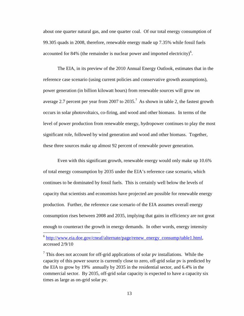
about one quarter natural gas, and one quarter coal. Of our total energy consumption of
99.305 quads in 2008, therefore, renewable energy made up 7.35% while fossil fuels
accounted for 84% (the remainder is nuclear power and imported electricity)6.
The EIA, in its preview of the 2010 Annual Energy Outlook, estimates that in the
reference case scenario (using current policies and conservative growth assumptions),
power generation (in billion kilowatt hours) from renewable sources will grow on
average 2.7 percent per year from 2007 to 2035.7 As shown in table 2, the fastest growth
occurs in solar photovoltaics, co-firing, and wood and other biomass. In terms of the
level of power production from renewable energy, hydropower continues to play the most
significant role, followed by wind generation and wood and other biomass. Together,
these three sources make up almost 92 percent of renewable power generation.
Even with this significant growth, renewable energy would only make up 10.6%
of total energy consumption by 2035 under the EIA’s reference case scenario, which
continues to be dominated by fossil fuels. This is certainly well below the levels of
capacity that scientists and economists have projected are possible for renewable energy
production. Further, the reference case scenario of the EIA assumes overall energy
consumption rises between 2008 and 2035, implying that gains in efficiency are not great
enough to counteract the growth in energy demands. In other words, energy intensity 6 http://www.eia.doe.gov/cneaf/alternate/page/renew_energy_consump/table1.html, accessed 2/9/10
7 This does not account for off-grid applications of solar pv installations. While the capacity of this power source is currently close to zero, off-grid solar pv is predicted by the EIA to grow by 19% annually by 2035 in the residential sector, and 6.4% in the commercial sector. By 2035, off-grid solar capacity is expected to have a capacity six times as large as on-grid solar pv.

14
(the ratio of energy to GDP) is expected to continue decreasing at a rate of 1.9% per year.
However, growth in GDP outpaces improvements in energy intensity, as GDP grows on
average 2.4% per year. Thus, even though energy efficiency improves, faster income
growth causes the overall level of energy demand to rise.
Measuring energy efficiency is not nearly as straightforward as measuring use or
market share of renewable energy. One of the difficulties with measuring efficiency is
that it can come in two forms: either reduced use of energy for a given service, or greater
service for the same amount of energy. The EIA has not yet identified a measure of
energy efficiency but instead uses energy intensity as a proxy. Energy intensity is a ratio
between energy consumption and gross domestic product or between energy consumption
and population.
Over the past 15 years, energy intensity in the U.S. has declined on average by 2.0
percent per year, and the EIA projects that this trend will continue, with energy intensity
declining by 1.9% per year from 2008 to 2035 (U.S. Energy Information Administration,
2010). However, GDP is expected to average 2.5% per year over the same period,
leading to an overall rise in energy demand. Energy intensity would have to fall more
rapidly (energy efficiency would therefore need to rise significantly) to offset the
projected rise in energy demand. The conservative efficiency assumptions in the EIA’s
Outlook therefore show a rise in overall energy demand. Other studies, however, show
that even with increased growth in population and GDP, energy demand could actually
fall by 2030 or 2050 through increased efficiency. Many researchers claim 25-30%
energy savings economy-wide are possible (see for example (Ehrhardt-Martinez &
Laitner, 2008) and (McKinsey Global Institute, 2007)). A comprehensive study on

15
energy efficiency conducted by the National Academy of Sciences found that “Energy-
efficient technologies for residences and commercial buildings, transportation, and
industry exist today, or are expected to be developed in the normal course of business,
that could save 30 percent of the energy used in the U.S. economy while also saving
money (National Academy of Sciences, 2010 (pre-publication copy)).”
Efficiency (or lower energy intensity) can be achieved in many ways: through
better energy use in the built environment (retrofitting existing residential and non-
residential buildings as well as more energy-efficient design of new buildings); through
appliance standards and use of more energy-efficient appliances; through changes in
energy-intensive industrial processes; and through increased use of mass transit and
changes in vehicle technologies.
Finally, while energy use per capita may be declining slightly, the U.S. still lags
far behind other industrialized countries such as Germany and France when we look at
carbon emissions per capita. This measure captures not only average energy use per
person, but specifically consumption of fossil-derived energy per person. In 2008, per
capita CO2 emissions in the U.S. were 19 metric tons, while in France they averaged 6.5
and Germany averaged 10.1. The U.S. also emits more carbon emissions per capita than
rapidly industrializing countries such as China and Japan. China’s per capita emissions
were only 4.9 metric tons in 2008 and India’s were 1.38. The differences between the per
capita emissions levels of these five countries stem from a combination of the mix of
energy sources used in each country as well as the per capita energy use. Most of the
differences result from the latter source. For example, if we focus on the electricity
8 U.S. EIA, International Energy Statistics

16
sector, the U.S. uses far more electricity per person than any of these other countries.
The U.S. averages 13,616 kilowatt hours (kWh) per capita while France averages 7,573
kWh/capita, Germany averages 7,185 kWh/capita, China 2,328, and India 543
kWh/capita9. In all cases but France, the level of electricity consumption correlates
closely with the level of per capita carbon emissions. And in all countries but France,
coal – the most carbon intensive energy source - is the main source of electricity. In
France, 77% of electricity comes from nuclear power, thus even though their per capita
electricity use is similar to Germany’s, their carbon emissions are much lower.
On a per capita basis, therefore, the U.S. uses much more energy than other
countries and produces more carbon emissions. The U.S. economy in 2008 was
responsible for 19 percent of global carbon emissions, even though the U.S. made up
only 4.5 percent of the global population10. These measures highlight the need for the
U.S. to reduce per capita energy consumption generally and consumption from fossil
fuels more specifically. Through implementation of energy efficient technologies and
energy efficient buildings, the U.S. can begin to reduce its energy use. And through a
switch to low-carbon and carbon-neutral energy sources such as wind and solar energy,
the U.S. economy can reduce its carbon emissions while sustaining economic activity.
Carbon Productivity
The concept of “carbon productivity” incorporates many of the issues raised
above. It incorporates both energy intensity and carbon emissions, since in essence it is
the inverse of the intensity of carbon use. In “The Carbon Productivity Challenge,”
9 International Energy Agency, Country Statistics, 2007 10 U.S. Census Bureau

17
McKinsey authors use the framework of carbon productivity to analyze the carbon
emissions abatement levels that will be necessary to meet the recommendations of IPCC,
Stern, and others (McKinsey Global Institute, 2008). "Carbon productivity" is the
amount of GDP produced per unit of carbon equivalent emissions (CO2e). To attain the
dual objectives of economic growth and reduced carbon emissions, we need to drastically
increase our carbon productivity. The authors estimate that to meet "common discussed
abatement paths [such as those outlined by Stern and IPCC]" we need a ten-fold increase
in carbon productivity, from $740 GDP per ton of CO2e today to $7,300 GDP per ton
CO2e by 2050” (McKinsey Global Institute, 2008, p. 7).
The Stern Review, discussed earlier, proposes a 2050 target of 20 gigatons of
CO2e to achieve 500 parts per million (ppm) concentration with no overshoot.11,12 To
meet this goal of emitting no more than 20 GtCO2e by 2050, along with achieving
continued economic growth of 3.1 percent per year (globally), McKinsey estimates that
global carbon productivity must increase ten-fold over the period.
McKinsey estimates that of the total abatement potential, 24% will come from
energy efficiency and 23% from growth in the use of renewable energy (the remainder is
attributable to behavioral change such as using more public transportation or lowering
thermostats, technological development which accelerates the conversion to renewable
energy, and increasing carbon sinks13). Energy efficiency investments will occur mainly
11 “Overshoot” means that this target can be temporarily exceeded before it is finally achieved. 12 Note here that gigatons of CO2e are an annual emissions rate, while 500 ppm is an atmospheric concentration of CO2.
13 “Carbon sinks” refer to parts of the eco-system which naturally absorb carbon. They can be expanded through avoided deforestation along with afforestation and reforestation.

18
in the industrial and residential sectors, followed by transformation (reducing energy
losses as we transform one energy source into another), then transportation and finally
commercial energy use. According to McKinsey, by 2020 we could save about 18 quads
(over 13 percent of global energy savings) in the U.S. through efficiency investments.
These energy savings will continue to grow through 2030 and 2050. Many studies, such
as the CCSP report, find that emissions reductions in the electricity sector come at a
lower price than in other sectors, and therefore efficiency improvement and
decarbonization will happen the most significantly in the electricity sector (Clarke, et al.,
2007).
Mitigation options presented by the IPCC include behavioral changes, carbon
pricing, and instituting a wide array of mitigation technologies, including but not limited
to: renewable heat and power; nuclear power; carbon dioxide capture and storage; more
fuel-efficient vehicles; hybrid vehicles; shifts in transport to rail and public transportation
or non-motorized options; efficient lighting and appliances; heat and power recovery in
industry; improved land management and cultivation techniques in agriculture;
afforestation; reforestation; composting organic waste; and landfill methane recovery
(IPCC, 2007, p. 60).
In their comparison of models that estimate the carbon dioxide mitigation
potential of various technologies, the IPCC finds that energy efficiency and conservation
offer the highest level of mitigation potential, followed by renewable energy, followed by
nuclear power and fossil-fuel switching, and finally carbon capture and sequestration
(IPCC, 2007, p. 68).

19
Energy-efficiency is the low-hanging fruit. As shown in abatement cost curves,14
many energy efficiency investments have so-called “negative costs”. That is, the
discounted flow of benefits resulting from the EE investments is greater than the initial
costs of those investments. “Negative costs,” in the EE literature, is another term for
positive value – namely the financial benefits resulting from savings on energy costs.
McKinsey estimates that approximately 7 gigatons of annual emissions would be at
negative cost to society, which is about one quarter of the abatement potential (McKinsey
Global Institute, 2008).
Another prominent strategy, decarbonizing energy sources, is comprised of
expanding renewable energy production, increasing use of carbon capture and
sequestration (CCS) technology (which McKinsey authors assume will not be
commercially viable before 2020), and reducing demand for oil and gas through more
fuel efficient vehicles and other technologies. Under McKinsey recommendations, with
currently available technologies, renewables themselves would grow from today's level
of 8% of supply to 23% by 2030. Because CCS is not expected to be commercially
viable before 2020, the decarbonization of energy sources can only happen through a
switch to renewable sources such as wind, water, and solar, and through reduced use of
fossil fuels. After 2020, CCS may also contribute to this strategy.
In this introduction, we have seen that carbon emissions have reached
unsustainable levels and that they must be reduced in order to maintain the health of our 14 The abatement cost curve shows the abatement potential (in levels of carbon emissions reductions) plotted against the cost of each abatement strategy. The McKinsey ACC ranges from “negative costs” for energy efficiency initiatives that have a very short payback period to high-cost strategies such as industrial carbon capture and sequestration.

20
planet and to avoid or reduce the economic damages that could result from climate
change. We have also seen that there is great potential for both energy efficiency and
renewable energy to reduce our carbon emissions through technologies that are currently
available. The question at hand is whether a shift to a more efficient and renewable
energy system can also contribute to the growth of employment. In the next chapter, we
review studies which address the employment impacts of a clean energy transition.

21
CHAPTER 2
LITERATURE REVIEW
Introduction
The majority of Americans (85%) believe that climate change is occurring, but
only slightly more than half of those believe it is attributable to human causes such as the
burning of fossil fuels. Among scientists, however, 84 percent find that climate change is
due to human activity, and 70 percent view it as a serious problem.15 Thus, there is
agreement approaching consensus in the scientific community, and significant
recognition in the general public, that climate change is present and problematic.
However, for the first time in 25 years, in March 2009 Americans responded to a Gallup
poll that focusing on economic growth is more important than tackling environmental
issues.16 An increasing number of economic researchers are focusing on the economic
impacts of climate change action, partly because any policy for reducing carbon
emissions will only have broad support if it also can improve economic well-being,
according to standard measures such as GDP per capita. Some of the analysis of global
climate change focuses on the costs of mitigation versus inaction, namely in terms of
GDP growth. Here we generally see Computable General Equilibrium (CGE) models
which forecast GDP (nationally or globally) over a long time horizon, such as the IAM
models discussed in the introduction. Other analyses focus on near-term and more
15 Pew Research Center, July 2009, http://people-press.org/report/?pageid=1550
16 http://www.gallup.com/poll/116962/americans-economy-takes-precedence-environment.aspx

22
regionally-specific economic impacts. These studies primarily use Input-Output (I-O)
models, case studies, or some combination of primary data used with an I-O framework.
Below I outline the various models used to estimate the economic impacts of climate
change, with particular attention to those used to analyze employment.
Estimating the Employment Impacts of Energy Policy
Overview of models
In a 2002 article, Peter Berck and Sandra Hoffman outline and describe various
modeling methods that can be used by economists and others to study the employment
impacts of environmental and natural resource policies (Berck & Hoffman, 2002).17
Berck and Hoffman outline five basic approaches to evaluating the effect of a policy
action on employment:
1. Supply and demand analysis of the affected sector; 2. partial equilibrium analysis of multiple markets; 3. fixed-price, general equilibrium simulations (input-output (I-O) and social accounting matrix (SAM) multiplier models); 4. non-linear, general equilibrium simulations (Computable General Equilibrium (CGE) models); and 5. econometric estimation of the adjustment process, particularly time series analysis.
17 These authors note the importance of analyzing impacts on the level of employment, rather than the unemployment rate per se, because of the implications and usefulness for politicians, who tend to have more impact on job creation than on the employment rate (which depends upon labor force participation).

23
Berck and Hoffman go on to describe the merits and drawbacks of each, and
further describe how each method operates. They note that the first two approaches
(single- and multi-market analysis) do not capture economy-wide impacts. I-O, SAM,
and CGE models represent a continuum of closely related models. They write:
I-O and SAM models provide an upper bound on employment impacts because their Leontief production functions do not allow for adjustment through factor substitution. For the same reason, they can be thought of as simulating very short-run adjustment. CGE models allow for factor substitution in response to changes in relative price. At an extreme, a perfectly neoclassical CGE model will have no aggregate change in employment, and therefore represents a lower bound on possible aggregate employment effects...More commonly, CGE models include migration or labor force participation equations that allow aggregate employment to change in response to changes in compensation.
In their assessment of linear models, Berck and Hoffman note that I-O and SAM
models are by far the most widely used models to assess employment impacts. SAM
expands upon the basic I-O model by including more detailed final demand sectors (such
as households at different income levels and governments at different levels).
In comparison to linear models, which are useful and most appropriate for short-
run analysis, CGE models build upon the I-O base by incorporating econometric
equations which model non-linearities such as factor substitution and technological
change. CGE models can therefore model the adjustment process and may be more
suitable to long-run forecasting (though not necessarily for employment, as we will see
below). However they are computationally expensive, generally including hundreds of
equations and significantly more data. Each relationship in the economy must be
modeled, and therefore is subject to data availability as well as the modeler's judgment.

24
While CGE models may be more suitable to long-run forecasting than the
simpler, more transparent I-O models which are at their core, CGE models must make a
number of assumptions in order for the model to ‘close’ – in order to reach a unique,
optimal, equilibrium solution. Neoclassical CGE models assume market-clearing
through changes in relative prices, assume that individuals are self-interested and act to
maximize utility, and that firms are perfectly competitive and therefore there is no real
profit in the system. In a CGE model, therefore, there is no involuntary unemployment,
as firms decide whether or not to hire workers based on the wages and the factor prices of
capital, energy, or other inputs, and individuals choose whether or not to work and how
much to work based on the wage they would earn in the labor market.18 Employment is
generally considered 'full' in CGE models since any change in employment levels does
not affect the unemployment rate – changes in wages affect the labor force participation
rate, not the unemployment rate.
Because the CGE model has an input-output foundation, both CGE models and I-
O models are capable of analyzing inter-industry linkages and determining output effects
resulting from changes in intermediate and final demands. However, the I-O model is
18 Heterodox CGE models, including structuralist models such as those developed and reviewed by Lance Taylor (1990), incorporate analysis of institutions and political economy, unlike neoclassical CGE models which generally rely on optimizing agents and full employment. In a structuralist CGE model, distribution (e.g. between wages and profits) matters, and employment and wages could both rise as workers gain more power. In a neoclassical CGE model, however, distribution and class power are not included in the analysis, and higher wages generally imply lower employment, as relative prices and factor substitution lead firms to substitute capital for higher-wage labor. The assumptions underlying these categories of CGE models can therefore lead to very different outcomes, and to my knowledge most if not all CGE models used to study climate change are built upon neoclassical foundations.

25
much simpler and more transparent, and because it does not require market-clearing
conditions, it is more suitable to studying questions of short-run employment changes.
Notably, I-O models do not assume full employment, and therefore a shift in demand (for
the outputs of one or more industry) may result in higher employment, even without a
change in wages. In the neoclassical CGE framework, more workers enter the labor force
in response to higher wages. But in the I-O framework, which does not make
assumptions about relative prices or assume full employment, some individuals may enter
the workforce out of involuntary unemployment, even without a change in wage inducing
them into employment.
While CGE models are dynamic and can be useful forecasting tools, mainstream
CGE models (such as those most often used to study climate change impacts) are
therefore not particularly well adapted to studying questions of employment impacts. In
the short run, in an economy with slack resources (such as unemployed individuals),
Input-Output models are better suited to studying employment impacts than are CGE
models. Because of the limitations of CGE models for studying these transitional
employment effects, I will not explicitly discuss any of these models here.
Above I situated various models within the framework of climate change policy
and action. In this dissertation, however, I focus my attention on investments in
renewable energy and energy efficiency (REEE), which will play an important role in
reducing carbon emissions. There is a small but rapidly growing body of literature on the
employment impacts of expanding the renewable energy and energy efficiency industry.
Much of the work undertaken in this area is done so either to combat the notion that there
is a trade-off in environmental and economic goals, or to present a clean energy path

26
toward meeting energy demands. Put another way, the question at hand is whether we
can further the agenda of environmental sustainability while also sustaining economic
growth. And if we can indeed meet our environmental and economic goals through a
program of expanded REEE, will expansion of this industry create decent employment
opportunities?
Within the existing body of literature that addresses these questions, I find that the
majority of studies are themselves literature reviews or presentations of summary
statistics with prose analysis. Only a handful of studies use empirical modeling to test the
hypothesis that an expanded REEE industry will generate growth in employment. We
will see that these latter studies make an important contribution towards developing a
methodology for quantifying the employment impacts of REEE, but that they are
constrained in their effectiveness because of limitations in the data. Below I focus on the
models that analyze employment impacts of REEE investments, as well as non-modeled
approaches such as case studies.
Input-Output and Linear Models
The most widely-used method to estimate the employment impacts of REEE
investments are input-output models or other linear models built on an I-O or SAM
platform, as mentioned above (Berck & Hoffman, 2002). Within the category of I-O and
linear models, we find two broad approaches.
The first approach estimates the employment resulting as a direct consequence of
investments in REEE technologies. Namely, the manufacture and installation of REEE

27
technologies will create employment in those industries that produce, install, and service
the technologies, as well as in industries with forward or backward linkages to the REEE
industries. This approach uses the I-O framework to simulate increased demand for
REEE goods and services and then estimates the economy-wide employment effects that
result.
The second approach uses the I-O framework but instead of estimating
employment resulting directly from REEE investments, this approach estimates the
energy savings that will accrue to users (households and businesses) and then uses an I-O
model to estimate the employment impacts of channeling those savings into other sectors.
Essentially, this approach models the employment impacts of changing industrial
spending patterns.
The I-O framework is useful for estimating “economy-wide” employment impacts
because it captures not only the employment created directly in the company producing a
good or providing a service, but the I-O model also captures employment in companies
throughout the supply chain. There are three categories of employment creation that
result from increased demand for the goods and services of any given industry. The first
is the direct effect - the personnel employed by the industry in question, such as the wind
turbine industry. The second level of employment creation is the indirect effect, which is
the employment in the industries that supply goods and services to the industry in
question, such as gearboxes and fabricated metal in the case of wind. Finally, we have
the induced effect - as employees in the wind and fabricated metal industries spend their
earnings, they generate demand for goods and services which in turn creates ‘induced’
employment. This induced effect is simply a way of specifying a consumption multiplier

28
generated by an increase in expenditures targeted at a specific sector, rather than an
economy-wide expenditure increase. To estimate the overall employment impacts
resulting from expansion of an industry, therefore, it is necessary to measure the direct,
indirect, and induced effects. The I-O model allows us to do just this, and thus to
estimate the economy-wide employment impacts of increased demand for renewable
energy and energy efficiency.
The majority of the studies presented below estimate only the direct and indirect
employment impacts of the REEE industry. Pollin et al. (2008, 2009), Scott et al. (2008),
Roland-Holst (2008), and The Perryman Group (2003) estimate these plus the induced
effects. All of these authors measure employment impacts by use of models built upon
an input-output framework. The detailed methodology of the input-output framework
will be presented in the next chapter. Here we will simply note that an I-O model allows
the user to estimate changes in output or employment through simulated changes in final
demand. If final demand for REEE output increases (say, households want to buy more
solar panels or businesses want to weatherize their facilities), then output and
employment will increase in the REEE industry itself as well as in other industries which
supply goods and services to the REEE industry. Researchers use the I-O model to study
both sectoral changes and economy-wide changes in employment.
The current I-O tables, however, do not recognize REEE businesses as
constituting an industry. Rather, these businesses have been classified as part of other
industries in the I-O tables. For example, we might find solar pv manufacturing
businesses as part of the electrical goods manufacturing sector, and building
weatherization as part of the construction industry. Despite the current data limitations,

29
some researchers have developed methods to analyze the economy-wide effects of
investment in the REEE industry in comparison to investments in other industries such as
oil refining or coal mining. Here we present this research, and later we expand the
methods previously used to study the REEE industry. While it is possible to estimate
direct employment in the REEE industry through extensive surveys, only the I-O model
allows us to study the indirect and induced effects, and thus to estimate the full economy-
wide impact. The studies reviewed below represent various attempts to estimate REEE
employment and to overcome limitations inherent in the I-O tables with current industrial
classifications.
Employment Created Directly through REEE Investment
In recent years, a number of authors have attempted to estimate economy-wide
employment resulting from REEE investments. While many studies focus on one
specific technology or industry, a few take a broader scope and analyze a combination of
renewable energy and energy efficiency investments.
We start with a study of the wind industry, conducted by the European Wind
Energy Association (2004). This multi-volume study analyzes all facets of the wind
industry in Europe. Here I concentrate on Volume 3, which focuses on employment and
market demand in the wind industry. The authors use I-O analysis and provide a detailed
description of the methodology used in assessing the direct and indirect employment
impacts of the manufacture, installation and operation of wind turbines. The authors use
input-output tables from Denmark, Germany, and Spain, the three countries which
provide 90% of Europe’s employment in the wind energy sector. As I mentioned above,

30
the European input-output tables (like the U.S. I-O tables) do not themselves include
wind energy or renewable energy as an industry. The authors therefore must supplement
the existing I-O tables, and do so with data gathered by surveying wind energy
associations in these countries. They do not directly expand the I-O tables. Rather, they
use information on the inputs to wind energy manufacturing, installation and operation to
estimate the direct employment effects, and then estimate the indirect requirements by
using employment multipliers from relevant intermediate goods-producing industries.
This study moves us closer to overcoming the data limitations inherent in the I-O
tables. The EWEA study collects data directly from wind energy firms and associations.
The authors can therefore assess more readily the direct as well as indirect employment
requirements of the wind energy. Of course, this study is restricted to wind and does not
include other renewable energy technologies or energy efficiency. However, the study
provides insight in how to proceed in gathering the appropriate data relevant to our
question.
Through interviews and survey data collected in 2003, the EWEA authors are able
to estimate that throughout Europe in 2002, approximately 31,000 people were employed
in wind turbine manufacturing, 14,650 in turbine installation, and 2,800 in maintenance.
In order to assess the indirect employment impacts, the authors rely on this same survey
data, plus assessments made by the national wind associations of Denmark and Germany,
as well as data from Eurostat’s input-output tables. By using survey data, the authors
determine the components involved in turbine manufacture. They then categorize these
components into industries which exist in the I-O tables and use the industry-appropriate
employment multiplier to arrive at a weighted average figure for indirect employment in

31
wind turbine manufacturing. They conduct similar exercises for installation and
maintenance.
The EWEA employment multipliers range from 8.2 jobs per €1 million in office
and data processing machines to 15.1 jobs per €1 million in metal processing. Like other
studies we review below, the EWEA study integrates a labor productivity estimate, which
they assume is the same across industries (unlike studies such as Hillebrand et al. (2006)
which assign industry-specific labor productivities). The authors conclude that direct
plus indirect employment in the wind industry in Europe in 2002 was approximately
72,000 people. Thus, the Type I multiplier would be about 1.5, which means that for
every job directly created in the wind industry, another ½ of a job is created in the
supplying industries. The authors estimate that wind creates 11.21 jobs per €1 million (in
2002) and that with productivity increases of 2 percent per year, by 2020 the wind
industry multiplier would fall to 7.79. This study restricts estimates to direct and indirect
effects and does not include induced effects. Despite this possible shortcoming, the
EWEA (2004) study makes an important contribution towards developing a method for
assessing the economy-wide employment impacts of an industry that is not recognized in
the existing input-output tables.
Another European study (Hillebrand, et al., 2006) evaluates the employment
impacts of renewable energy in Germany. In this paper, the authors model the economic
effects of increasing the share of renewables in electricity, from 5% to 12% by 2010.
They find that there are competing effects - on the one hand, there is an expansionary
effect from investment, which is greater in the early years in some industries and in the

32
later years in others, and then they find a longer-term contractionary effect resulting from
increased electricity prices.
The authors augment the static I-O model to include dynamic effects such as price
changes, substitution, and changes in government revenues and spending. Their
integrated model includes a goods model, a price model, a capital stock accounting
segment, a labor market model and a redistribution model. Hillebrand et al. note that
investment effects will lead to economic and employment growth, and that expansion of
renewable energies will involve additional investments in production facilities in addition
to transportation and distribution facilities. "The main beneficiaries of these investments
are the investment goods industries, especially the sectors concerning electrical and
optical equipment, construction, and machinery, all of which will face decreasing
investment amounts over time. In contrast, the fabricated metal products industry will -
although on a substantially lower level - increasingly benefit from the expansion of
renewable energies. This is mainly due to the rising number of new photovoltaic
installations (p. 3487)." The employment effect is therefore stronger in earlier years than
in later years, due to declining new employment from new production facilities. The
government budget will have positive impacts from two sources. First, tax revenue will
increase from new businesses and new employment. Second, the positive employment
effects will lead to decreased public expenditures for welfare programs or other transfer
programs.
In the short-run, therefore, Hillebrand et al. estimate that there will be a net gain
in employment economy-wide. In the longer term, however, employment will rise more
slowly and may eventually decline. The cost effect of using more renewable energy is

33
what leads to somewhat of a contraction in employment. The authors assume that since
renewable energy is more expensive than conventional energy, that electricity prices will
necessarily rise. They take no account (or at least make no mention) of the fact that
renewable prices might actually fall when these technologies become more diffuse, or
that technological innovation might result in lower-cost renewable technologies and
therefore lower electricity prices. The contractionary effects that they find, therefore, are
likely greater than they would find if they assumed a more modest price increase, or if
real electricity prices stayed relatively constant to today's level.
The EWEA and Hillebrand studies focus only on renewable energy technologies,
and do not include energy efficiency. Next I review three studies which take a more
comprehensive view of REEE investments and attempt to measure economy-wide
employment impacts, including direct, indirect, and induced employment.
The first set of studies I review in this group are produced the Political Economy
Research Institute (Pollin, Heintz and Garrett-Peltier (2009); Pollin and Garrett-Peltier
(2009); Pollin et al. (2008)). In these studies, my co-authors and I use the framework of
the EWEA report to model economy-wide investments in REEE. Specifically, we create
a ‘synthetic’ REEE industry by assigning industries and weights to various components
of REEE technologies. We can then simulate increased demand for REEE goods and
services and estimate the resulting employment impacts. I will return to a detailed
discussion of this methodology in Chapter 5, since this provides us with a reasonable
framework for estimating the employment effects of REEE investments, despite the non-
existence of this industry in public I-O tables. Here I will note that the Pollin et al.
studies model a ‘green program’ which consists of investments in building weatherization

34
(40%); mass transit and freight rail (20%); smart grid, wind, solar, and biomass (10%
each). Each of these industries in turn is composed of various manufactured goods
(fabricated metal, electrical goods, etc.) and services (construction, technical services,
and so on). We find that on average, each $1 million of investment in REEE creates 16.7
jobs economy-wide, compared to only 5.3 in fossil fuels (oil, gas, coal), and that a shift to
REEE will create a large number of jobs economy-wide. For example, a $150 billion
investment shift from fossil fuels to REEE would lead to a net increase of 1.7 million
jobs. This includes the creation of 2.5 million jobs in REEE, minus the contraction of
800,000 in fossil fuels, if spending in fossil fuels decreased by the same amount as
spending in REEE increased (Pollin, Heintz, & Garrett-Peltier, 2009). The I-O model
used by Pollin et al. is a static model, which means it is valid for short-term estimates but
does not include dynamic effects such as price changes and factor substitution. As
pointed out by Berck and Hoffman (2002), it may thus represent an upper bound of job
creation. However, since 70% of the REEE investments in Pollin et. al are targeted to
energy efficiency, which lead to energy cost savings which can be channeled to other
productive purposes, the overall employment effect may actually rise, indicating that
these estimates are not necessarily an upper bound.
In 2009, Roger Bezdek , under commission from the American Solar Energy
Society, estimated the employment impacts of various environmental policies using a
method similar to that used by Pollin et al. (Bezdek, 2009). This study is an extension of
an earlier study led by Bezdek, "Tackling Climate Change in the U.S.", in which the
authors assess the potential for reducing carbon emissions in the U.S. through
deployment of REEE technologies. In this 2009 report, Bezdek estimates the job impacts

35
of those earlier recommendations. He uses input-output modeling as well as an
occupation-by-industry matrix to predict occupational outcomes.
Bezdek finds that from 2007 to 2030, the REEE industry could quadruple,
creating a net gain of 4.5 million jobs in clean energy over the period. The increased size
of the renewable and efficiency industry is the result of an aggressive policy scenario
designed to reduce carbon emissions to 80% below 2005 values by 2050. The net
changes in energy spending and jobs account for the losses in conventional energy
production coupled with a rise in REEE-related spending and employment. The job
estimates themselves are derived through input-output modeling, and are essentially the
jobs per dollar of REEE investments minus the jobs per dollar of fossil fuels, times the
total cost of the REEE deployment. In order to estimate total costs, the authors consider
deployment curves for each technology (how many units of energy output or efficiency
are produced or saved annually by each technology), then estimate the deployment cost in
each year of deployment. These costs, in turn, account for supply curves, R&D, and
learning curves, and the analysts use life-cycle cost analysis to estimate the cost per year
for each technology. In estimating job impacts, the authors take into account these
factors and adjust production functions so that the number of jobs created in solar, for
example, will rise from 2020 to 2030, but in wind the number will fall. The total number
REEE jobs will continue to grow from 2020 to 2030, and the largest segment of job
creation is in energy efficiency.
Finally, I will mention the work done by the Perryman Group, who estimated
employment impacts for the Apollo Alliance, an alliance of businesses and non-
governmental organizations that advocates for a transition to a clean energy economy.

36
The Perryman Group (herein TPG) produced a set of employment estimates using a
proprietary model built upon an I-O base (The Perryman Group, 2003).
The TPG report, while not as detailed in the methodology as the EWEA report, is
nonetheless useful in that it provides an example for assessing the economy-wide job
impacts of a massive expansion of both renewable energy and energy efficiency. The
Apollo Plan calls for public investment in a broad package of energy reforms. The
Apollo Alliance (at the time this report was written) recommended a “10 Point Plan”
which includes the following:
• $30 billion in regulations and incentives to strengthen renewable energy markets, such as guaranteeing production tax credits and creating federal matching funds
• $6 billion to support development of bio-energy, including increased funding for R&D and demonstration programs
• $30 billion in production tax credits and subsidies to increase production of American-made fuel-efficient vehicles
• $42 billion in tax incentives to increase energy efficiency in manufacturing • $42 billion for green building tax credits • $34 billion to support the Low Income Home Energy Assistance Program • $20 billion to develop new transit infrastructure • Other funding to support hydrogen fuel cell RD&D, to develop the electrical
transmission grid, to increase appliance standards, to finance energy-efficient home improvements, to fund brownfield redevelopment, to provide support for regional planning, to develop high-speed rail, to upgrade existing transportation networks, to upgrade municipal water infrastructure. This funding includes a variety of R&D, tax policy and direct expenditures.
The Perryman Group estimates that the effects of the proposed Apollo plan
investments of $313 billion over a 10-year period include the addition of $1.35 trillion in
Gross Domestic Product and 19.4 million person-years of employment (cumulative).
This increased GDP is the result of targeted federal spending which leverages additional
private spending. Federal spending of $313 billion over the 10-year period leverages

37
additional private spending, for total cumulative expenditures of close to $3 trillion.19 Of
this, $1.35 trillion is additional GDP while the remainder is intermediate costs. This is
the cumulative amount, thus for each year of the program, expenditures equal close to
$300 billion (combined public and private), and close to 2 million jobs are supported
economy-wide (including direct, indirect, and induced employment).
The methodology used by TPG (2003) is based on an input-output framework.
Estimates of direct spending on programs in the Apollo project were provided to the
Perryman Group by the Apollo Alliance, and were then used in the I-O table
manipulations. TPG has a proprietary model called the US Multi-Regional Impact
Assessment System (USMRIAS). They describe it as follows:
The USMRIAS is somewhat similar in format to the Input-Output Model of the United States and the Regional Input-Output Modeling System, both of which are maintained by the US Department of Commerce. The model developed by TPG, however, incorporates several important enhancements and refinements. Specifically, the expanded system includes (1) comprehensive 500-sector coverage for any county, multicounty, or urban region; (2) calculation of both total expenditures and value-added by industry and region; (3) direct estimation of expenditures for multiple basic input choices (expenditures, output, income, or employment); (4) extensive parameter localization20; (5) price adjustments for real and nominal assessments by sectors and areas; (6) measurement of the induced impacts associated with payrolls and consumer spending; (7) embedded modules to estimate multi-sectoral direct spending effects; (8) estimation of retail spending activity by consumers; and (9)
19 The explanation of the methodology and assumptions used to derive this leveraging ratio as well as the total effects on GDP are not discussed in the Perryman report. The inputs used by Perryman are “corroborative” and their model is proprietary, therefore it is not possible to examine their spending, GDP, and employment levels in any depth.
20 The term “extensive parameter localization” is not described in the Perryman methodology paper, and is a term with which I am otherwise unfamiliar.

38
comprehensive linkage and integration capabilities with a wide variety of econometric, real estate, occupational, and fiscal impact models. The models used for the present investigation have been thoroughly tested for reasonableness and historical reliability (pp. 9-10)21.
Thus, this study builds upon some of the previous work in this field by using a
model that captures direct, indirect and induced effects. TPG uses data from the BEA,
the BLS and the ACCRA Cost of Living Index for regional spending patterns (to capture
induced effects). However, we should be cautious in analyzing the results.
Unfortunately, as mentioned above, we cannot decipher the specific effects on
employment that expansion of the REEE industry would generate. Like the studies
previously reviewed (with the exception of EWEA (2004)), TPG does not have access to
data on the REEE industry that they could incorporate into their input-output analysis.
There does not appear to be any direct surveying of renewable energy firms, and it is
unclear how the Perryman Group arrives at its job estimates for investment in renewable
energy. For other sectors, they may have reasonable proxies, such as energy efficiency
through home weatherization being proxied by home re-modeling, or the manufacture of
hybrid vehicles being proxied by auto manufacture. Perryman can thus make reasonable
estimates of energy efficiency industries, but can only cite other sources when discussing
the job impacts of wind and solar technologies. While TPG uses an input-output
framework, their model is proprietary and therefore the assumptions and results cannot be
verified.
21 The authors do not explicitly describe the types of tests used to assess “reasonableness and historical reliability”.

39
The five sets of studies reviewed above use similar methods to estimate
employment. The first (EWEA) focuses only on wind, the second (Hillebrand et al.) on
renewables more generally, and the last three sets (PERI, Bezdek, TPG) take a more
comprehensive approach, modeling direct, indirect, and induced effects of employment
created by expanding both renewable energy and energy efficiency. All of these studies
use a jobs-per-dollar approach to analyzing investments in REEE. That is, they estimate
how many jobs will result from a given level of spending in the clean energy economy,
and in some cases, such as Pollin et al. and Bezdek et al., analyze the effects of a dollar-
for-dollar shift from fossil fuel spending into clean energy spending.
Employment Created through Energy Savings
The next set of studies also uses an input-output framework, but instead of
analyzing jobs that result from clean energy investments, as the above studies do, these
studies instead estimate the energy savings that will result from efficiency investments,
and then channel those savings into other sectors and analyze the net job impacts of this
shift in the distribution of spending. This type of study is typified by John “Skip” Laitner
(multiple studies) and Roland-Holst (2008). The premise of these works is that the
traditional energy sector is capital-intensive, and that households and businesses that
reduce their energy expenses will spend those savings in other sectors which are more
labor-intensive. Thus the dollar-for-dollar shift from utilities, transportation fuels, and
other energy goods, into other (more labor-intensive) sectors, will create a positive
employment effect.
40
Since energy efficiency is not an industry or sector categorized in the existing I-O
tables, Laitner et al (1998) try to overcome this constraint by using the I-O model to
estimate employment impacts by hypothesizing how alternative energy efficiency
scenarios would change consumption and thus production patterns across industries. The
authors estimate the direct and indirect employment created by an increase in final
demand. This will necessarily understate the total employment effects of a given change
in final demand, since it does not include the employment resulting from the increased
earnings and consumption by households (the induced effects).
To estimate the direct and indirect multipliers, Laitner et al. (1998) use the 1993
IMPLAN model (IMpact analysis for PLANning) which was developed by the Minnesota
IMPLAN Group. Using this model, the authors can compare the total number of jobs
both directly and indirectly created within the United States. They find, for example, that
multipliers are lowest in industries such as refining, utilities, oil and gas extraction, and
motor vehicles – industries which have low labor-intensity in production. The multipliers
are highest in industries such as education, government, agriculture, and financial
services – industries with high labor-intensities of production.
There is, as previously mentioned, no REEE industry in the current I-O tables,
and therefore no multiplier for the REEE industry. In order to capture the employment
impacts of increased energy efficiency, Laitner et al. make some assumptions as to how
spending will change among the sectors contained in the I-O tables. They assume, for
example, that 90% of efficiency investments would be spent in the United States, they
make assumptions about labor productivity (sector-specific), they assume that 80% of the
investment upgrades would be financed by bank loans and that 15% of investment in

41
building and industrial sectors would go towards marketing expenditures. The labor
productivity estimates were calculated from BLS projections, and the values for financing
were taken from an earlier study by Geller et al (1992). There was no discussion of the
value chosen for domestic versus international efficiency investments. After making
these financing and spending assumptions, the authors then apply them to the existing I-O
tables to determine the employment multipliers resulting from these changes in final
demand. Having obtained these employment multipliers, they can then determine which
industries would be net “winners” or “losers” of jobs. They find, for instance, that jobs
will decline in electric utilities, oil and gas extraction, and wholesale trade; while jobs
will increase in retail trade, government, construction and financial services. Over their
12-year projection, which is from 1998 to 2010, they predict that the net employment
gain economy-wide is 772,859 jobs, that compensation and salaries will increase by $14
billion and that GDP will increase only slightly, by $2.8 billion. Unlike other I-O studies
of REEE investments, the results obtained by Laitner et al. are not derived from the
investments themselves, but rather from the cost savings that accrue to businesses and
households as a result of implementing more energy-efficient technology. As their
energy bills decrease, businesses and individuals re-spend these savings in other sectors
of the economy which are more labor-intensive than the energy sector, therefore driving
up economy-wide employment.
Barrett et al. (2002) conduct a somewhat similar exercise. Like Laitner et al.
(1998), they use an existing model to forecast the employment impacts of changes in
energy use. Specifically, they outline a policy scenario that calls for:

42
1. A $50 per ton carbon tax, mostly offset by a payroll tax cut;
2. policies to promote energy efficiency and renewable energy technologies as
well as policies to offset competitive impacts on energy-intensive industries ;22
and
3. transitional assistance to workers and communities (approximately $100,000
per worker).
The authors then use the LIFT (Longterm Interindustry Forecasting Tool) model
to forecast employment impacts under this set of policies. The LIFT model was
developed in the 1960s by the Inforum modeling group at the University of Maryland,
and is a 97-sector macromodel of the U.S., built upon an I-O base. Using the LIFT
model and their adjustments, they find that GDP would increase very slightly (at most
0.6% by 2020), and that 660,000 net jobs would be created by 2010 and 1.4 million by
2020 (which is about 1% of the 2002 workforce). The primary factor driving these job
gains are reductions in the cost of production (due to energy efficiency gains).
Furthermore, after-tax compensation would rise. Their findings are thus roughly
comparable to those of Laitner et al (1998), using a similar methodology.
In 2007, Laitner et al. extend the 1998 analysis of jobs created through energy
efficiency. The authors develop and use a model they call "DEEPER" (Dynamic Energy
Efficiency Policy Evaluation Routine) which they describe as "quasi-dynamic" since it
22 The policy package used in the Barrett et al (2000) study is based on the scenarios created by the U.S. Department of Energy in their Interlaboratory Working Group (2000) report entitled “Scenarios for a Clean Energy Future.” The moderate scenario comprises policies such as information outreach efforts, enhanced R&D, government procurement programs, voluntary industry agreements, technical assistance, stricter codes and standards, feebates, rebates, and tax credits. The advanced scenario expands upon the moderate scenario by including a carbon permit trading system as well increasing government financial involvement.
43
adjusts energy costs based on the level of energy quantities produced in a given year, and
it adjusts labor impacts given the anticipated productivity gains within the key sectors of
the Texas economy (Laitner, Eldridge, & Elliot, 2007). The DEEPER model is an Excel-
based tool that consists of the following modules: global data; macroeconomic model,
which includes the 15-industry I-O based model from IMPLAN; investment and savings;
price dynamics; final demand; and results.
As in the Laitner et al. (1998) study, the authors here estimate direct and indirect
employment multipliers, and keep households exogenous in the model. They use a 15-
industry breakdown, and show employment impacts resulting from $1 million in final
demand (for example, 20.4 jobs in agriculture, 3.8 in oil and gas extraction, 2.4 in electric
utilities, 13.5 in construction). Their overall job impacts are estimated by doing the
following: They assume a zero 12-year change in investment; over this period, they
estimate what the job impact would be if $1 million was transferred from other types of
spending into installing energy-efficiency equipment, and $1.5 million was saved on
energy bills and spent elsewhere in the economy. Installing energy efficiency
improvements would generate 13.5 jobs per $1 million (this is exactly the employment
figure from construction) and diverting this money from elsewhere would reduce jobs by
11.9 (it is not clear in the report where this figure comes from). Reducing utility revenues
would decrease employment by 2.4 jobs per million (therefore 3.6 jobs for $1.5 million)
but the money spent elsewhere would increase jobs by 11.9 per million (again, unclear
where this comes from) and thus create 17.9 jobs per $1.5 million. The overall
employment effects of these transfers of spending are thus 15.9 jobs created per $2.5
million energy-efficiency investments and spending shifts. Laitner et al. conclude that in

44
the first year, the job impact of their policies prescriptions for the state of Texas would be
5,573, a number which just about doubles every five years and reaches 38,291 by 2023.
This represents a gain of only 0.3% in the state's employment base.
By sector, the authors note that the four big winners are construction,
manufacturing, services and financial services. This results because these sectors benefit
from initial investments in EE and also because these sectors will experience higher
demand for goods and services as savings from energy bills are re-spent throughout the
economy. Again, the Laitner et al. (2007) study must make assumptions about changes
in spending patterns to be able to forecast employment changes due to energy efficiency
improvements. Like the aforementioned studies, this report is useful in estimating
changes in spending that result in changed employment patterns.
In a very recent study, Laitner evaluates the historical evidence on energy
efficiency improvements and uses a 'diagnostic tool' to show the outcomes on GDP and
employment of using other models with baseline scenarios, typical modeling scenarios
(climate change policies as modeled by the EPA and others), and scenarios using
American Council for an Energy-Efficient Economy (ACEEE) assumptions of increased
efficiency investments (Laitner, 2009). The ACEEE assumptions lead to greater GDP
and employment over the period from 2009 to 2050, and imply a decrease in energy
intensity and thus a savings in energy use of about 25-30 percent. These EE investments
have a short payback period and lead to savings which are channeled to other sectors. As
in earlier work, Laitner uses IMPLAN to model the employment multipliers for energy,
manufacturing, services, construction, and government. All of these sectors are more

45
labor-intensive than energy. Thus a shift from spending in energy into any other sector
will increase employment.
Reference case scenarios in Laitner (2009) show energy demand and prices rising,
and thus total energy spending rising. Laitner demonstrates that typical energy modeling
(as done by EPA and others) results in a rise in energy prices, and a rise (though slower)
in energy demand, resulting in higher overall energy spending in 2050 versus 2009. The
ACEEE case shows a net fall in energy demand, so that even with a slight rise in energy
prices, total energy spending is lower in 2050 than it is today. Energy prices rise more
slowly in this scenario than in the baseline case because of lower demand for energy.
Laitner’s ‘diagnostic tool’ shows that in the reference case the total resource cost is $4.2
trillion and would rise to $4.9 trillion in the typical model. But with ACEEE assumptions
it in fact falls to $2.7 trillion. This lower energy cost (-$1.5 trillion) leads to a positive
net impact on GDP of $456 billion, rather than a net fall in GDP of $229 billion.
Laitner cites work by the Union of Concerned Scientists (Cleetus, Clemmer &
Friedman 2009) which contains a "detailed portfolio of technology and program options
that would lower U.S. heat-trapping greenhouse gas emissions 56 percent below 2005
levels in 2030. The result of their analysis indicated an annual $414 billion savings for
U.S. households, vehicle owners, businesses, and industries by 2030." The net savings to
the economy are on the order of $255 billion per year. Over the 20-year period, the net
cumulative savings are on the order of $1.7 trillion.
Having evaluated the assumptions and outcomes from various models used to
estimate employment impacts of climate change policy, Laitner (2009) points to the

46
drawbacks of using CGE models to analyze these questions. He notes that CGE models
fail to value many co-benefits associated with climate solutions (such as non-energy
productivity gains23, improved energy security, better air quality, improved public
health), and that they operate under assumptions of rationality and perfectly competitive
markets (and as we noted above they also operate under the condition of full
employment). Finally, most CGE models use fossil fuel prices as they are currently
structured, which means that they are under-priced since they do not account for
environmental externalities.
Over the longer term, the results in Laitner (2009) are similar to those in Pollin,
Heintz, and Garrett-Peltier (2009). Both studies analyze the predictions of EPA and other
environmental models, which show that even under their own assumptions, by 2050 there
is only slightly slower GDP growth – not, in fact, a decline in GDP. In other words, GDP
grows in all scenarios, reaching levels far above today’s. Climate change policies as
typically modeled would only lead to a slight postponement (of a few months) in
reaching a certain level of GDP over 40 years (reaching the same level of GDP per capita
by July 2051 instead of sometime in 2050). The Laitner (2009) study also shows that
ACEEE case (of more substantial efficiency investments) would lead to a slight
acceleration in GDP growth (reaching the reference case scenario by Aug 2049). The
important illustration in both studies is that in all the modeling cases, the economy
23 Productivity gains, like the other benefits mentioned here, are referred to as “co-benefits” – in this case, benefits attributable to energy efficiency investments that are not directly energy- or cost-related. Non-energy productivity might increase in this case as energy cost savings are channeled into capital equipment or other investments that enhance productivity.

47
continues to grow, just slightly faster or slower depending on assumptions used in the
model.
Another study that uses an approach similar to Laitner (2009) is by David Roland-
Holst (2008). The Roland-Holst study is a policy analysis of past and future energy
efficiency policies and other climate change policies in the state of California. The
author focuses on the household sector in this state, since household consumption is
responsible for 70% of the state's GSP and therefore is a leading driver of state energy
use24. Roland-Holst uses a modified I-O approach that incorporates the effects of climate
change policies and innovation.
While he is particularly interested in modeling the effects of AB 32, California's
"Global Warming Solutions Act," Roland-Holst also evaluates historical energy
efficiency in CA in comparison to the rest of the U.S. Using national and state I-O tables,
he finds that from 1972 through 2006, about 1.5 million jobs were created as the result of
$56 billion worth of energy savings that were spent in other sectors. (This yields a
multiplier of 26.8 jobs per $1 million.) Net, he finds that for every job lost in the fossil
fuel sector, 50 jobs were gained in others. These estimates are much higher than those
predicted by Laitner et al. (in multiple studies) as well as those predicted by Pollin et al.
or others using the I-O methodology.
24 Since households purchase from the building, commercial, and transportation sectors, this approach captures most energy-related transactions. However it excludes one major user of energy and producer of emissions – the industrial sector, from which households do not buy directly.
48
Though he used an I-O model to estimate historical energy policy, Roland-Holst
models the future employment effects of AB32 using the BEAR model (Berkeley Energy
and Resources) created by CERES (the Center for Energy, Resources, and Economic
Sustainability) at UC Berkeley. This is a CGE model that incorporates emissions and
innovation. Using BEAR, Roland-Holst finds that by 2020, emissions goals under AB 32
can be met, and up to 403,000 new efficiency and climate action jobs will be created.
This modeling approach is similar to Laitner et al., in that it analyzes the job gains from
shifts in spending from the capital-intensive energy sector into more labor-intensive
sectors (such as retail and food service). However it differs in that it uses a CGE model.
Given the usual full-employment assumption of CGE models, it is unclear how Roland-
Holst is able to predict employment changes. Though not explicitly stated in his paper, if
employment rises in a CGE model it is due to an increased labor force participation rate,
which may result from more people entering the workforce in response to higher
compensation or migration. However, if this is what drives Roland-Holst’s results it is
not explicitly stated in the report. Nonetheless, Roland-Holst, like all of the studies
mentioned so far here, predicts a net gain in employment resulting from implementing
energy efficiency policies.
Finally, a study commissioned by the Department of Energy’s Office of Energy
Efficiency and Renewable Energy uses an I-O based model and performs an analysis
similar to that of Laitner (Scott, et al., 2008). The authors were commissioned to
evaluate the economic impacts of building technology programs, which include energy
efficiency upgrades to residential and commercial buildings. The authors develop an I-O
based model from BEA data that is modified to account for changes in energy use as well

49
as changes in capital stock, investment, and productivity more generally. They use a
188-sector model, and find that the FY2005 building technologies program could save
27% of the expected growth of building energy use by 2030, creating 446,000 jobs and
increasing wage income by $7.8 billion. The authors also find that over the period there
will be significant energy and capital cost savings which can be channeled into
consumption (residential savings) or productive investment (commercial savings).
Scott et al. note that there is debate over the macroeconomic impacts of energy
efficiency programs, namely because of distributional effects (across industrial sectors).
Energy bill savings will have positive effects on most sectors but negative effects on the
energy sector, giving an uncertain net effect (ex ante). The authors situate their model
within the range of models enumerated by Berck and Hoffman (2002) and after
reviewing alternative methods, choose to use the I-O approach because it "lends itself
readily to analyses of technologies for residential and commercial buildings."
ImSET (the 188-sector model developed by Scott et al.) tracks the corresponding
changes to inter-industry purchases of goods and services (and energy in particular), and
recalculates the use matrix and the consequent changes to the input-output structure of
the economy in each forecast year. This differs from most I-O models, in which a
constant I-O structure is usually applied to a change in investment. Savings in the
energy, labor, materials, and services from improved energy productivity are the source
of subsequent rounds of investment and economic growth. We can therefore view this
study as spanning our two categories above - it estimates job creation both from initial
investments in efficiency as well as from energy savings and shifts in spending.

50
Finally, once they have obtained the new vector of output, Scott et al. apply
capital/output ratios and investment/output ratios for each sector to estimate the savings
in capital expenditures that would accrue from energy efficiency investments. For
example, increased efficiency reduces the demand for power plants, pipelines, etc. and
thus reduces capital expenditures in those areas, which can be channeled into other (more
productive) investments.
We note that within this category of studies (those that model the effects of
shifting spending), all of these authors analyze only energy efficiency investments, and
do not model renewable energy concurrently. The methodology assumes that financial
savings from energy efficiency result in job creation. This type of analysis may or may
not be transferable to studying renewable energy, since in shifting from fossil fuel energy
to renewables, overall spending on energy may increase or decrease depending on
technological diffusion and changing costs of RE. If RE becomes less expensive than
fossil fuels are today, then households and businesses might see cost savings that they
can channel elsewhere. However if RE remains more expensive than conventional
energy, energy bills may rise, causing a shift in spending to energy from other sectors.
Thus it will be important to examine the labor intensity of RE. Knowing this, we can
model the employment effects in a shift from fossil fuels to RE. While this is not done
by Laitner and others in the category of studies presented here, it is in fact analyzed by
Pollin, Heintz, and Garrett-Peltier (2009), and we will pursue this methodology below.
51
Non-Modeled Employment Analysis
The studies presented above use a variety of modeling approaches to estimate
REEE employment. Here, I present some alternate methods which use case studies
(primary data) as well as secondary data in order to estimate direct employment, and in
some cases indirect employment, in various renewable energy technologies. Generally,
these studies use a “jobs-per-energy-unit” rather than a “jobs-per-dollar” approach. That
is, rather than estimating the cost of a technology and then using an I-O model to estimate
employment created by expenditures, these case studies and other non-modeled
approaches estimate how many jobs are needed to produce a given RE technology with a
given energy production capacity. For example, how many jobs will be created if a
company receives an order to produce a 10 megawatt wind turbine? While these studies
do not examine economy-wide employment effects, they are nonetheless useful in
assessing employment needs for increased production of RE goods.
Case Studies
The first set of studies which use primary data is typified by Kammen et al. In
2004, Kammen, Kapadia, and Fripp published a review of 13 alternative studies of
renewable energy and employment. They analyze the main assumptions and models in
these 13 studies, and compare estimates of employment in the manufacturing and
operations of renewable technologies, based on jobs per MWa (average megawatt). The
authors conclude that over a broad range of scenarios, "the renewable energy sector
generates more jobs than the fossil fuel energy sector per unit of energy delivered."
52
In 2009, Daniel Kammen extends this approach, and together with Engel Ditley of
Vestas (a large wind energy firm) produces a policy brief comparing jobs in wind energy
to those in fossil fuels (on a jobs-per-MW basis). This brief highlights some of the
findings from a paper by Kammen and others (2010, described below), and showcases
some examples of jobs and economic activity in the wind industry, namely at current and
planned Vesta wind technology manufacturing plants. Kammen and Ditley (2009) also
review an in-depth study by the European Wind Energy Association showing that wind
creates more jobs per MW than fossil fuels. Finally, they also showcase a recent
McKinsey & Co. analysis showing that wind creates more jobs per MW than coal, gas,
and nuclear power. This 2009 review of wind energy studies shows that on a job-per-
MW basis, renewables (in this case wind) generate more jobs than fossil fuels.
Then in 2010 Kammen and others perform a meta-analysis of about 15 other
clean energy and jobs studies, and also offer a methodology for comparing employment
estimates that were derived by different methods (Wei, Patadia, & Kammen, 2010).
They then offer an open-source analytical tool that can be used to model the employment
effects of varying renewable portfolio standards (RPS) and energy efficiency measures
from 2009 to 2030.
The methodology follows the usual Kammen et al. strategy of comparing jobs per
MW across various technologies. This particular study limits itself to the power sector,
with attention to evaluating various levels of a national RPS. The authors also attempt to
estimate net job creation, with attention to job losses in coal and natural gas25. In order to
25 The authors model the effect of an RPS, which applies to electricity. Since coal and natural gas are the primary fossil sources of electricity, and oil contributes minimally, the

53
make other estimates comparable, the authors convert all job estimates into job-years per
average MW. First they convert all the CIM jobs (Construction Installation
Manufacturing) into job-years over the life of the plant (so for example they divide the
total estimate of CIM jobs by 25 if the plant life is that many years). Next they use
capacity factors to ensure that they can compare employment per unit of energy between
technologies that have different capacities. Having made the estimates comparable, they
find that renewable energy and low-carbon technologies create more jobs per MW than
fossil fuel technologies, and that solar pv creates the most.
They note that most jobs studies only include direct employment, or might also
include indirect, but rarely if ever include all three levels (direct, indirect, induced). In
their own analysis, they estimate direct and indirect effects for RE but add induced for
EE, which they admit will bias the results in favor of EE. Since they report total results
and do not separate induced effects from direct and indirect, readers are not able to
directly compare the direct and indirect effects of renewable energy to energy efficiency.
In the energy efficiency sector they assume that the majority of jobs are from induced
effects (90%) with only 10% of the jobs resulting from the actual manufacturing or
installation of EE products.26 For the RE indirect multiplier, they use an average across
all technologies of 0.9 (they obtain this value from 3 other studies). This is of course not
authors restrict their attention to job losses related to the electric power sector, namely those in coal and natural gas.
26 This is similar to the Laitner et al approach, which assumes that most employment gains from energy efficiency will result from a shift in spending from the energy sector into more labor-intensive sector. Here in the Wei, Patadia, and Kammen study, the authors refer to this as ‘induced’ job creation.

54
industry-specific and most likely there is variation across the technologies that an I-O
approach could distinguish but theirs cannot.
Their methodology does not account for leakages (especially manufacturing jobs
that are offshore) and does not account for regional differences or local versus national
analysis. They note that their model would also benefit from including learning curve
effects, since jobs in 2030 will likely be lower than their estimates because of
technological innovation. Under one back-of-the-envelope learning scenario, this could
lead to a multiplier that is 17% lower in 2020 (Wei, Patadia, & Kammen, 2010).
Case Studies Combined with Secondary Data
Finally, the Renewable Energy and Policy Project (REPP) has developed a non-
modeled approach which incorporates primary and secondary data, as well as some of the
methodological elements presented above. In earlier studies (Singh & Fehrs, 2001),
REPP conducted surveys of RE firms to estimate direct jobs in those firms and compare
jobs-per-MW between renewable technology production and fossil fuels. In subsequent
studies ( (Sterzinger & Svrcek, 2005), (Sterzinger, 2006)) they include an indirect
multiplier and also use BEA data to indentify employment within the supply chain of
renewable technologies.
Singh and Fehrs (2001) estimate the direct labor requirements of the wind, solar,
and biomass industries by conducting written and phone surveys of one or more firms in
each industry, in addition to data provided in industry journals. They estimate various
types of jobs, including those in parts manufacture, delivery of goods to power plants,
construction/installation/project management, operation and maintenance for 10 years,

55
and cultivation and collection of biomass fuel. They also offer an overall cost
comparison of coal, wind and solar PV. They estimate that for a given $1 million of
expenditure, coal generates 3.96 person-years of employment over 10 years, wind 5.70
and solar PV 5.65. Per megawatt of electricity, solar photovoltaic (pv) supports 35.5
person-years, wind supports 4.8 and biomass co-firing can range from 3.8 to 21.8 person
years (with co-firing from mill residues on the low end and co-firing from switchgrass
and poplar on the high end).
By conducting surveys of firms in these REEE industries, Singh and Fehrs (2001)
are able to determine the occupational mix for the labor requirements of renewable
energy technologies. They group jobs into 10 categories, which are the following:
professional/technical/management; clerical/sales; service; agriculture/forestry;
processing; machine trades; benchwork; structural work; miscellaneous. These
categories do not correspond directly to the occupational categorization of the BLS.
However, this is nonetheless a useful exercise – both because it highlights the importance
of surveying to gather the relevant data and also because having a sense of the
occupational mix is important in understanding what types of jobs will result from an
expansion of REEE.
In the 2005 study by Sterzinger and Svrcek, the authors use wind-industry data to
identify the components and costs of wind turbine manufacturing (similarly to the EWEA
2004 study). They then assign NAICS codes (North American Industrial Classification
System) to each component so that they can use publicly available data to estimate
current employment levels in each component industry. However this only measures
employment in firms which could manufacture wind turbine components, rather than

56
those that are currently producing for the wind industry. For example, the authors
measure employment in “motors and generators” which could be inputs into wind
turbines or could be used by other industries such as automobile production. While this
study is useful in identifying the relevant industries for the production of renewable
energy technologies, the authors are unable to distinguish which part of each industry is
unique to renewable energy and which part services other industries and end uses. This is
yet another example of the limitations of currently available data, which make it nearly
impossible for researchers to use secondary data (such as BEA or BLS) to study RE
employment.
In 2006, Sterzinger goes one step beyond this 2005 research and attempts to
estimate jobs resulting from various RE technologies, both directly and indirectly. This
more recent report (Sterzinger 2006) is the result of a project to update the "jobs
calculator", a spreadsheet tool used to calculate jobs resulting from varying Renewable
Portfolio Standards (RPS). The industries included in the RPS and calculator are wind,
solar, biomass, and geothermal. The jobs estimates (jobs per MW) were derived in a
similar way to PERI’s 'synthetic industry' approach. Sterzinger identifies the components
of each technology, matches those to NAICS codes, assigns cost shares to each of those,
and calculates total costs per MW for each NAICS category. Then he uses a jobs/MW
number (based on surveys and interviews) to get a total number of jobs. Since Sterzinger
provides both total job estimates and total costs, we can use these to calculate jobs/$ and
compare this to results that researchers obtained using input-output analysis.
Sterzinger’s results show 6.39 jobs/$1million in wind, 4.28 in solar, 4.72 in
geothermal, 6.16 in biomass, and an average (from total investment of $160.5 billion and

57
total FTE jobs of 850,603) of 5.30 direct jobs per $1 million from these four
technologies. Since Sterzinger uses a direct job-per-MW approach, these estimates do
not include indirect or induced effects. However Sterzinger does identify the relevant
components and costs of these four technologies, and could therefore use an input-output
model to estimate economy-wide employment effects. Here, as in the other REPP reports
presented in this sector, the focus is on renewable energy and does not include energy
efficiency.
Advantages and Disadvantages of Renewable Energy Case Studies
The studies and methods presented in the section above have the advantage of
using actual data from the field, such as the number of workers employed in a given wind
turbine manufacturing firm, which may in some cases be more useful or accurate than the
more aggregated data in the I-O models. I-O models rely on data which are collected
from millions of firms and then aggregated into various industries. Thus in using I-O
models we are essentially working with industry averages, which may not always be
reflective of the experience of individual firms. However, there are also some
disadvantages to working only with case study data. First, for the most part these studies
only measure direct job creation, and do not enable us to evaluate the economy-wide
impacts of a technology. Similarly, this method does not allow researchers to examine
net job impacts, since we cannot estimate either economy-wide job gains from RE
investments or economy-wide losses in fossil fuel employment. Finally, these studies
generally are conducted for only one technology or a limited range of technologies, and
may not be broadly applicable to investments in the full spectrum of renewable energy
and energy efficiency. These studies are useful, however, in providing data that other

58
researchers can use to derive economy-wide employment impacts, for example, by
integrating the data into an input-output model.
Discussion of Choice of Input-Output Model
In this dissertation, I have chosen to employ the input-output model to study
employment impacts of REEE investments. This is due both to the advantages of the I-O
model that are discussed above, as well as the drawbacks of using other approaches. The
I-O model allows us to estimate economy-wide impacts of investments in a range of
REEE technologies, and thus has useful macroeconomic implications. Further, it also
allows us to evaluate the effects on specific sectors and industries, which is useful for
industrial policy as well as employment, training, and readjustment policies.
In the past decade, as we can see from the studies surveyed above, economists
have expanded in various ways the input-output methodology used in employment
impact analysis. As we will see below, the I-O methodology has existed for over 70
years now, but has only recently been applied to questions of renewable energy and
energy efficiency. The authors discussed above demonstrate how this methodology can
be used to examine direct and indirect impacts, and how the basic I-O framework can be
extended to include induced effects, price effects, productivity changes, and so on.
However, many of the studies had to make significant assumptions about the composition
of the REEE industry or changes in economy-wide spending patterns, since the REEE
industry does not exist as such in the current I-O tables. The EWEA (2004) tries to
overcome this limitation by conducting extensive surveys of relevant firms and
associations to estimate direct effects and then using the I-O model to estimate indirect

59
effects. However, this is relevant only to the wind industry, and only in Europe. No
survey of this magnitude has been conducted in the United States, and to my knowledge,
no survey of REEE businesses throughout the U.S. has yet been conducted. Thus,
previous research is limited in the estimates it can make and comparisons it can draw
regarding employment in REEE.
While significant research on this topic has been underway and continues to grow,
there remain many holes to fill in the literature. This dissertation contributes to the REEE
literature in a number of ways. First, it extends the methodology used by the EWEA and
Pollin et al. to identify an REEE industry within the current I-O tables. Second, I conduct
a nationwide survey of REEE firms in the U.S. to expand the data and our knowledge of
the REEE industry, and finally I incorporate that data into the BEA’s current I-O tables to
estimate the employment impacts of REEE investments and compare those to spending in
fossil fuels. Through this data collection and methodological extension, I will contribute
to the literature by providing an alternative estimation of REEE employment.

60
CHAPTER 3
USING THE INPUT-OUTPUT MODEL TO STUDY RENEWABLE ENERGY AND ENERGY EFFICIENCY
The Input-Output Model
Background
Wassily Leontief, known as the father of input-output modeling, developed this
framework in the 1930’s, based on the “tableaux economiques” by Francois Quesnay in
the 1750’s. Leontief created input-output modeling and used it for impact analysis as
early as 1936. Input-output tables are national accounting systems that show linkages
between industries and that allow us to see how changes in final demand can affect
industrial output both directly and indirectly ( (Leontief, 1986), (Miller & Blair, 1985),
(Stone, 1961)).
Input-output tables for the U.S. economy are compiled by the Bureau of
Economic Analysis (BEA) of the U.S. Department of Commerce. Every five years, in
years ending in ‘2’ or ‘7’, the Census Bureau gathers data (in its “Economic Census”) and
the BEA uses these data along with information from other Census Bureau programs—
including annual surveys that cover selected industries, such as manufacturing and
services. The I-O tables also incorporate data collected and tabulated by other Federal
agencies—including the U.S. Departments of Agriculture, Education, and Energy—and
data from a number of private organizations (Horowitz & Planting, 2006). In their
comprehensive manual on the BEA input-output accounts, Horowitz and Planting (2006)
write that:

61
The Economic Census collects most of the essential data required for the tables—such as receipts, inventories, and payrolls—and the data are collected at the level of the smallest operating unit, the “establishment.” In addition, the Census Bureau’s collection procedures are designed to ensure that no individual establishment is counted more than once. Thus, by relying on the Economic Census data wherever possible, BEA is able to limit duplications that could occur when the Economic Census is used in conjunction with other sources. While the Economic Census is wide-spread and covers millions of establishments,
it nonetheless relies on sampling of small businesses, and some establishments and
industries are not included in the Census. Therefore the BEA supplements these Census
data with information from other establishment surveys conducted by other agencies as
well as by the Commerce Department itself. This includes data from the agricultural
sector collected by the US Department of Agriculture, data on fossil fuels and utilities
collected by the Energy Information Administration of the U.S. Department of Energy,
data on the financial industry from the Securities and Exchange Commission, on
insurance from the A.M. Best Company (an insurance rating company that compiles
financial information on insurance companies), and data on education from the
Department of Education’s Digest of Education Statistics. The BEA also uses two of its
own sources to supplement these outside data sources. It draws from the NIPA (national
income and product accounts) for a variety of domestic transactions, and the ITA
(international transaction accounts) for imports and exports.
The Economic Census itself, which makes up the backbone of the I-O accounts,
was first established in 1810 and consisted of a few questions on manufacturing. It has
grown to include over 500 versions of the questionnaire, and collects data from 3.7
million businesses representing over 5 million business establishments in over 1,000
industrial classifications. In addition, the Census Bureau uses administrative records to

62
compile information on 14 million businesses without paid employees plus 1.5 million
small-business employers (Horowitz & Planting, 2006).
The BEA uses the data collected from these various sources to construct
benchmark input-output tables for close to 500 industries. Between the quinquennial
census years, the BEA updates the benchmark tables to produce annual input-output
tables at more aggregated levels. In order to perform these annual updates, the Census
Bureau compiles samples of companies and conducts a variety of annual surveys. These
include the Annual Survey of Manufactures, the Annual Wholesale Trade Survey, the
Annual Retail Trade Survey, and the Service Annual Survey which covers various
service industries. In addition, BEA uses data from the Census Bureau’s County
Business Patterns, Business Expenses Survey, construction statistics program, and two
programs covering government activities – the Census of Governments and the Annual
Survey of Government Finances (Horowitz & Planting, 2006).
The input-output tables compiled from these various establishment surveys
provide a “snapshot” of the economy. In any given year, they show the inputs used by
each industry, the outputs produced by each industry, and the relationship between
industry output and final demand among various users. The I-O tables, both at the
benchmark level as well as the annual tables, include a “make” table (the commodities
produced by each industry), a “use” table (the use of commodities by intermediate and
final users), a “direct requirements” table which is an algebraic manipulation of the make
and use tables showing the amount of a commodity required by an industry to produce a
dollar of the industry’s output, and a “total requirements” table which is also known as
the “Leontief Inverse Matrix,” described below.

63
The basic structure and subsequent algebra for the input-output model are
presented here. We start with a flow table, F, which is an (n x n) matrix showing the
dollar value of goods and services which are exchanged between the n industries in the
model. Adding along a column of the flow table will yield the total inputs (in dollars)
used by each industry. Adding along a row will yield the total dollar value of output
produced by each industry.
To calculate the proportionate use of goods and services that each industry uses of
the other industries (and its own products), we need to calculate the coefficients matrix
(A), which is derived by dividing each cell of the inter-industry flow table (Fij) by the
total industry output of that particular industry (Xj):
aij = Fij/X j
where Fij stands for an element in the flow table and aij is the corresponding
element in the coefficients matrix (A), with i and j running from 1 to n. The element aij
therefore represents the input (product of industry i) into the production of one unit of
output of industry j.
The coefficients table (A), when post-multiplied by the vector of total output (X),
yields the intermediate (industry) demands for goods and services. The basic equation
for the input-output model is then
X = AX + Y

64
where X is an n x 1 column vector of total output for each of n industries, AX is
the output to meet intermediate demand (with the dimensions of A being n x n and the
dimensions of X being n x 1), and Y is an n x 1 vector of final demand.
Rearranging the equation above to solve for final demand, we obtain
X-AX = Y
Since we are interested in observing how a change in final demand (Y) will affect
output (X), we then isolate output as well:
X(I-A) = Y,
where I is the identity matrix, then
X = (I-A) - 1Y
where (I-A)-1 is the Leontief inverse matrix which I will describe and use below
to study output and employment impacts.
The input-output model I will use here to study the REEE industry is based on the
BEA 2006 annual tables at the 65 industry level. The BEA “Total Requirements” table,
or Leontief inverse matrix, shows how an increase in demand for a particular industry’s
product will lead to increased output in that industry and all related industries. For
example, an increase in demand for farm products would increase farm output and would
also increase output in other industries which provide inputs to the farm industry, such as
fertilizer and farm machinery manufacturing. The total requirements table will be an n×n
matrix where n is the number of industries. Once we obtain this table, we can post-
multiply it by a vector of final demand (Y) to estimate the effects on output (X). Thus

65
our basic equation to estimate a change in output resulting from a change in final demand
is:
∆X = (I-A) -1∆Y
Using this impact equation, we can see how changes in alternative types of final
demand (personal consumption, private investment, federal government expenditures, or
exports) affect output. We can also isolate a change in final demand for one industry or a
group of industries (for instance, increased healthcare spending by the federal
government) to estimate the economy-wide impacts of such a demand shock.
Estimating Employment Multipliers Using the Input-Output Model
To study the effects on employment, rather than simply output, we convert our
Leontief Inverse Matrix into an Employment Requirements Table. This table is used to
estimate the number of jobs throughout the economy that are needed, both directly and
indirectly, to deliver $1 million of final demand for a specific commodity. In order to
create the employment requirements table, we first need to obtain employment/output
ratios for each industry in the model. We can obtain gross output by industry as well as
full-time-equivalent (FTE) employment by industry from the BEA tables27. These data
are available at the 3-digit level of the North American Industrial Classification System
(NAICS). The industries in the I-O tables are also classified according to NAICS codes,
27 Gross output and FTE employment are found in the “GDP-by-Industry” files maintained by the BEA and available here: http://www.bea.gov/industry/gdpbyind_data.htm

66
which is an industrial classification developed jointly by the U.S., Canada, and Mexico,
and which has been used since the 1997 Economic Census.
Within the NAICS system, industries are classified at increasing levels of detail,
starting with 2-digit sector level detail (e.g. NAICS 11 = Agriculture, forestry, fishing,
and hunting), and becoming more detailed with each additional digit (e.g. 111=crop
production; 1111=oilseed and grain farming; 11111=soybean farming). The 6-digit level
NAICS is the most detailed industry level, and it is this level of detail which is obtained
every five years in the Economic Census. From the 6-digit level, industries can be
aggregated up to 2-digit through 5-digit levels. The I-O tables are created at three levels:
Sector; Summary; and Detail. The sector-level tables correspond to 2-digit NAICS
categories and contain 15 industries. The summary-level tables correspond to 3-digit
NAICS categories and contain 65 industries. Finally the benchmark, or detailed tables,
correspond to the 5-digit NAICS categories and contain 477 industries.
Here I choose to work with the summary level tables (65-industry) for two
reasons. First, the size of these tables is more tractable and this will become an important
factor as I integrate new data into the existing tables (discussed in subsequent chapters);
and secondly, the benchmark (477-industry) tables are only produced every 5 years, and
the most recent version available is from 2002 (the tables are released with a 5-year lag
due to the intensive activity of converting statistics from various sources into the I-O
tables). The summary tables are updated annually, as described above, and therefore
tables from more recent years are available. I will work with the 2006 summary-level I-
O tables.

67
In their national industry accounts, the BEA provides estimates of gross output by
industry in 2006 as well as full-time-equivalent (FTE) employment by industry in 2006 at
the 3-digit NAICS level of detail, which is the level we need in order to generate
employment/output ratios for each of the 65 industries in the BEA input-output tables. I
generate an employment/output ratio for each industry, which is simply the total FTE
employment for each industry divided by that industry’s gross output in the same year, in
this case 2006. I then form a diagonal 65×65 matrix with the employment/output ratios
along the diagonal and zeros elsewhere, which I call “e.”
To create the employment requirements table, E, I take the diagonal matrix of
employment/output ratios, e, and post-multiply it by the Leontief inverse matrix, or total
requirements table, as follows:
E = e(I-A) - 1
Where (I-A) – 1 is the Leontief inverse table and e is the diagonal matrix, both of
which have the dimension 65×65.
The employment requirements table shows us both the number of jobs directly
created and indirectly created, as a result of demand for a particular industry’s product.
For example, if demand for farm production is $1million, we can immediately see both
the number of farm industry jobs (direct jobs) supported by this demand, as well as the
number of jobs supported in other industries such as fertilizer and farm equipment which
supply inputs to farms (indirect jobs).
The employment requirements table is the foundation of my analysis, and I will
use it to see how changes in spending can affect jobs throughout the economy. While the

68
Leontief inverse matrix yields output requirements and an output multiplier, the
employment requirements table yields employment requirements and an employment
multiplier. Each industry will have a unique multiplier.
We can use this framework to see how an increase in spending in any industry (an
exogenous increase in demand, which could result either from private or public spending)
will generate jobs. The basic impact equations are:
∆X = (I-A) -1∆Y (to measure change in output); and
∆X = E∆Y (to measure change in employment).
The employment multipliers from this static model include both direct and
indirect employment resulting from a given type of demand. The direct employment
effects are found along the diagonal of the E matrix. The indirect effects for a given
industry are the sum of all of the values in a column of the E matrix, minus the direct
value along the diagonal. In table 3 I present employment multipliers from a selection of
industries within the standard 65-industry BEA I-O model from 2006.
As we see from table 3, the employment multipliers for different industries within
the I-O model can vary quite a bit, with a low of 0.64 direct jobs per $1 million demand
in oil and gas extraction, a very capital-intensive industry, to higher values such as the
13.80 jobs/$1million found in administrative and support services, a much more labor-
intensive industry. As described in detail above, the employment multipliers are the
result of two factors: employment/output ratios and inter-industry transactions (captured
in the Leontief inverse matrix).

69
Mathematically, it is clear that the multiplier of a given industry will be large if
the employment/output ratio is high, if the level of inter-industry transactions (output
multiplier) is high, or if some combination of the two occurs. More generally, however,
we can trace the causes of differences in employment multipliers to three main reasons:
labor intensity; domestic content; and compensation to workers. Labor intensity is
captured by the employment/output ratio. In comparison to industries that are capital-
intensive, labor-intensive industries will employ a greater number of FTE workers for the
same level of output. Secondly, an industry will have a higher employment multiplier the
higher its share of domestically-produced inputs is. This is captured within the inter-
industry table. A higher domestic content implies that more output, and therefore more
employment, is created within the domestic economy, rather than being imported or
outsourced and creating output and employment in foreign economies. Since the inter-
industry table measures the extent to which domestic industries supply goods and
services to each other, a higher domestic content will be captured in this table. Thirdly,
all else equal an industry will have a higher employment multiplier if average
compensation is lower. For example, if $1 million in final demand generates $600,000 in
total compensation (and the remainder in other inputs), and average compensation is
$30,000, then 20 FTE workers will be employed. However, if the $600,000 is paid out to
workers earning on average $60,000, then only 10 FTE workers will be employed. Thus
in general any difference between industries’ employment multipliers can be traced to
some combination of differences in labor intensity, domestic content, and worker
compensation. Industries with higher labor intensity, higher domestic content, and lower
compensation, will have higher employment multipliers.

70
Assumptions Embodied in the Input-Output Model
Miller and Blair (1985) note that the two main assumptions in input-output tables
are those of fixed technical coefficients and fixed input proportions. Fixed technical
coefficients means that the inter-industry flows from industry i to industry j depend
entirely on the output of industry j. In other words, if the output of industry j doubles, its
input from industry i will also double. Fixed proportions implies that industry j will use
the same mix of inputs from all industries even as demand increases for industry j 's
output. That is, the production function, which is a Leontief minimization function, is
homogenous. Rather than a classical production function which assumes diminishing
marginal returns, the Leontief production function assumes constant returns to scale. The
returns are fixed by technology, and technology is assumed to remain constant as output
grows. The BEA refers to these two assumptions as the principles of homogeneity and
proportionality.
We must keep these assumptions in mind when conducting any impact analysis
with the I-O tables. First, this suggests that I-O tables are best suited to studying the
current state of the economy and making short-term projections and we should therefore
exercise caution when using I-O models to conduct long-range forecasts. In the long-
term, we would expect technological change to occur, which would change the
production function and therefore the factor proportions. Furthermore, the assumption of
constant returns to scale is relevant only for relatively small changes in levels of output.
If an industry increases output by, say, 5 or 10 percent, we might be able to assume
constant returns to scale. But a doubling of the size of the industry, such as we might
expect to occur with renewable energy, will no doubt lead to changes in the returns to
71
scale alongside changes in technology. Thus, we should exercise caution in using input-
output models for forecasting purposes, and any forecasts we may want to conduct in
future work should no doubt include integrated models built on a dynamic input-output
framework which incorporates changes in production functions.
Furthermore, because the Census is an “economic snapshot,” the resulting I-O
tables themselves are static. Thus, we must be aware of not only homogeneity and
proportionality, but also of fixed prices. If, over time, input prices change, then we
would expect industries to substitute cheaper inputs for the more expensive inputs.
The limitations of the input-output model lie in these three assumptions
(homogeneity, proportionality, and fixed prices) which are of course made for
simplification as we know that no industry operates in this type of environment. Its
strength, however, lies in the simplicity of the model and the relatively limited number of
assumptions in comparison to more complex general equilibrium models which typically
rely on a far greater number of assumptions.28 Richardson (1972) says that part of the
appeal of the I-O model is that it is “value-free” and “neutral” and thus is useful for
economic impact studies in a wide variety of settings – from capitalist to planned
economies.
Input-output tables can essentially be used in one of three ways: To determine the
current state of economic interactions (static); to change assumptions regarding
production functions or prices, or to change final demand (comparative static); or to
28 For example, typical assumptions in CGE include profit-maximization, perfect competition, market-clearing conditions, production at full capacity, and full employment.

72
incorporate technological change or permit expansion of the economy by introducing
capital coefficients into the framework (dynamic). Here we will be using the input-
output model for comparative static analysis. Namely, we will study the employment
effects of an increase in final demand for REEE products and services.
Creating “Synthetic” Industries in the I-O Model
Background and Motivation
As previously noted, within the 65 industries in the BEA there is no ‘Renewable
Energy’ or ‘Energy Efficiency’ industry. The only energy-related industries which are
identified in the BEA I-O model are oil/gas extraction, coal mining, support services for
these extraction activities, power generation and distribution, and various petroleum- or
coal-based manufacturing activities. Renewable energy technologies such as wind, solar,
biomass, geothermal, and so on, are not explicitly identified. Energy efficiency industries
such as building weatherization, “Smart Grid”29, energy-efficient appliances, and so on
are also not explicitly identified. Nonetheless, the activities of these industries are
captured implicitly in the input-output accounts. For example, the manufacture of
hardware and electrical equipment used for solar panels are categorized respectively in
the hardware and electrical equipment industries. If we can thus identify the various
29 “Smart Grid” is a term used to describe a modernized electricity transmission infrastructure which relies on information-technology to increase reliability and reduce demand of the electrical grid system. The Smart-Grid is more interactive and distributed than the current electrical grid in that it allows end-users to interface with power use through ‘Smart Meters’ and allows for more de-centralized power production (such as wind and solar) to be distributed to users. For more information, see for example publications by the U.S. Dept. of Energy’s Office of Electricity & Energy Reliability, accessible here: http://www.oe.energy.gov/smartgrid.htm.

73
components and their weights that make up the REEE industry, we can study the impact
of increased demand for REEE products and services. The methodology for what I am
calling the ‘synthetic industry approach’ is presented in Miller and Blair (1985).
The synthetic industry approach may serve as a placeholder strategy or a viable
alternative strategy to gathering survey data and explicitly identifying the REEE industry
and expanding/updating the existing BEA I-O tables, which I will discuss in chapters four
and five. The integrated approach presented in subsequent chapters models both forward
and backward linkages between various industries, thus the REEE industry is both a
consumer and producer of goods and services in the integrated approach. In the synthetic
approach presented here, however, we simulate an exogenous increase in final demand
for the goods and services used in the REEE industry. Thus here the REEE industry is
essentially a consumer of goods and services (all of the inputs that go into the
manufacture of wind turbines, for example), but is not a producer from which other
industries purchase. Therefore we only capture linkages in one direction and cannot
capture the full set of economic interactions. After presenting this approach below, and
the integrated approach in chapter 5, I will discuss the results and merits of each method
in chapter 6.
The motivation and precedent for using the synthetic industry strategy to study
renewable energy is developed in the EWEA’s study of the European Wind market
(European Wind Energy Association, 2004). This comprehensive study, discussed
earlier, includes information on the components and costs of wind turbine production as
well as employment in the wind energy industry. The authors undertook a survey of
various European firms in the wind energy industry. Through this process they gathered

74
data on the direct employment in wind energy firms, along with the data that would allow
them to use EuroStat’s Input-Output accounts to measure indirect employment. To do so,
they categorize the wind energy components into industries which exist in the I-O tables
and use the industry-appropriate employment multiplier to arrive at the figure for indirect
employment in wind turbine manufacturing. They conduct similar exercises for
installation and maintenance.
The EWEA methodology not only motivates the survey which we conducted and
will discuss below, but also offers guidance as to how to use existing I-O tables along
with information on REEE components to derive REEE employment multipliers. The
EWEA publication shows that for wind turbine manufacturing, the various components
and weights are as follows:
37% machinery 26% construction 12% fabricated metal products 12% plastic products 7% scientific/technical services 3% mechanical power transmission equipment 3% electronic connector equipment
Using these weights along with our basic employment impact equation,
∆X = E∆Y
we can analyze the effects of an increase in demand for wind turbine production.
If our change in demand, ∆Y, is $1 million, then the increased demand for industrial
production in the I-O model is:

75
$370,000 machinery $260,000 construction $120,000 fabricated metal products $120,000 plastic products $ 70,000 scientific/technical services $ 3,000 mechanical power transmission equipment $ 3,000 electronic connector equipment
Using these industries and spending amounts, we can thus estimate the effects on
employment (or on output) of a $1 million increase in demand for wind energy
production. These above shares include the manufacture of wind turbines, which the
EWEA estimates to be 74-82% of the total cost of new wind power, as well as associated
construction costs and other services. Similarly, we can use information we gather about
the component costs of various REEE industries to create a final demand vector (or
change in final demand, ∆Y). This will allow us to study the effects of expanding the
REEE industry without having an REEE industry explicitly identified in the I-O tables.
Recent Applications
To my knowledge, the only studies which have used this approach – the analysis
of synthetic REEE industries using the I-O model – have been those co-authored by
myself along with other economists at the Political Economy Research Institute (PERI) at
the University of Massachusetts, Amherst30. In the PERI studies we have used this
approach to model various clean energy investments both in the U.S. (at the national,
regional, and local levels) and in Ontario, Canada. We have also used this framework to
30 See, for example, Pollin, Heintz & Garrett-Peltier (2009, June); Pollin and Garrett-Peltier (2009, April); or Pollin et al (2008, Sept.).

76
model other investment or spending programs such as infrastructure and military
spending. We return to these studies below.
Other authors have conducted similar exercises but without using all parts of this
methodology. For example, the Renewable Energy Policy Project conducted a report for
the state of Ohio in which they identify all of the components of various manufactured
clean energy technologies (wind, solar, geothermal, biomass), along with investment
amounts, to forecast employment growth in each of those industries based on certain
funding levels (Sterzinger & Svrcek, 2005). However, the authors of this report did not
use the components and costs in tandem with the input-output accounts, but rather used a
rule-of-thumb number of jobs for all of the industries (3000 FTE jobs per $1 billion
investment) and applied that to the spending in each component industry. Thus the only
industry-specific employment effects result from differences in spending levels per
industry, not differences in labor intensity or production functions.
Using the input-output model along with the spending-by-industry information
yields richer detail and arguably more accurate estimates, since it allows us to estimate
industry-specific employment outcomes in addition to economy-wide outcomes.
Whereas the Sterzinger & Svrcek paper uses a rule-of-thumb 3000 FTE jobs per $1
billion investment for all of the component industries, within the I-O model we could
estimate a jobs/dollar value for electronic goods, for electrical equipment, for fabricated
metal, and so on. We could then use a weighted-average jobs/dollar that would reflect
both the employment and spending specific to producing wind turbine components. This
may be lower or higher than the Sterzinger & Svrcek rule-of-thumb, but it is certainly
more rigorously derived, since the production functions of various wind energy

77
components are likely to differ from one component industry to another, and therefore
our employment estimates will be more accurate than a rule-of-thumb estimate.
Two examples of papers which use the synthetic industry approach to estimate the
employment effects of REEE investments are “The Economic Benefits of Investing in
Clean Energy” (Pollin, Heintz, & Garrett-Peltier, 2009) and “The U.S. Employment
Effects of Military And Domestic Spending Priorities” (Pollin & Garrett-Peltier, 2009).
In each of these papers, we use alternative specifications for green investments in order to
compare them to various other domestic spending programs. In the first paper, we
compare the job creation effects of various energy efficiency and renewable energy
investments (building retrofits, mass transit/rail, smart grid, wind, solar, and biomass) to
fossil fuel investments (oil/natural gas and coal). The job creation estimates from each
$1 million investment are presented in figure 1. In order to obtain these estimates of
direct and indirect job estimates, we use an input-output model and define the ‘synthetic’
REEE industries and fossil fuel industries as presented in figure 2.
Thus we use the synthetic industry approach to analyze REEE industries within
the I-O model and generate employment estimates that are directly comparable with
fossil fuel industries. In the 2009 paper by Pollin and Garrett-Peltier, we compare clean
energy investments with a variety of domestic spending areas such as military spending,
education, health care, and tax cuts for personal consumption. While military spending,
education, health care, and personal consumption are all sectors identified within the
standard I-O model, the clean energy industry of course is not. However, the synthetic
industry approach allows us to estimate the employment impacts of clean energy in a
manner consistent with developing our estimates for the other spending areas. Our

78
synthetic “clean energy” industry is the same as the “green program” in previous work,
such as the 2009 Pollin, Heintz, Garrett-Peltier paper previously mentioned. The “green
program” or “clean energy” industry in these works consists of 40% building
weatherization, 20% mass transit/rail, and 10% each of smart grid, wind, solar, and
biomass investments. Each of these industries was in turn developed using the synthetic
industry approach with the weights as listed in the above figure.
Testing the Validity of the Synthetic Industry Approach
The synthetic industry approach allows us to perform impact analysis for
industries which do not currently exist in the input-output model. To my knowledge,
there are no formal tests we can use to gauge the validity of this technique. There are
other methods we could use, however, to see if our estimates are reliable. Two such
methods include surveying/interviewing large numbers of firms in the industry in
question, and performing specification tests with our synthetic industry components and
weights.
In the first instance, we would use a survey of industry members to assess
whether our employment estimates derived through the synthetic industry approach
correspond with reported employment in REEE businesses and organizations. That is, if
we predict that $1 million demand for wind turbines will generate X number of jobs in
wind production, do wind turbine manufacturers actually employ X number of workers
for each $1 million in revenue? Since the input-output model is based on industry
aggregates, we would need to survey a large number of firms to find the average values
among them and to see if they correspond with our model’s predictions. In chapter six I

79
will perform such a test. However in general it is impractical to gather this survey data to
test the synthetic approach, since the approach is generally necessary precisely because
we do not have sufficient survey data.31
The next method we could employ to test the validity of our construction of
synthetic industries is to perform various specification tests. That is, we can create
alternative specifications for each industry in question by varying the weights of the
component industries to see how sensitive the results are to the choice of specification.
Since there is no distribution of values, we cannot measure standard deviations or use
other population distribution measures. Here I will simply calculate the various impacts
generated by alternative specifications, compare those impacts to each other, and then use
a rule-of-thumb to determine whether or not the results are sensitive to the specification
of the synthetic industry.
I use here the example of the wind industry, created by Pollin, Heintz & Garrett-
Peltier (2009) based on the EWEA wind industry weighting scheme (European Wind
Energy Association, 2004). I first reconstruct the original direct and indirect multipliers
using the original weighting scheme then create two alternative specifications. In the first
alternative weighting scheme, I increase the total share of the non-manufacturing
industries by ten percentage points and decrease the share of manufacturing industries by
31 Currently, in fact, PERI researchers are conducting exactly such an exercise with data from recipients of Dept of Energy grants and contracts awarded as part of the American Recovery and Reinvestment Act of 2009. PERI researchers used an input-output model to estimate employment resulting from a variety of Recovery Act programs, and now the awardees are reporting jobs created/maintained by these programs, allowing the researchers to compare estimates to reported job counts. However, typically this type of data is not available to test the validity of I-O employment estimates.

80
ten percentage points. In the second alternative specification, I increase the share of
manufacturing industries and decrease non-manufacturing, each by ten percentage points.
The alternative weights and resulting employment impacts are presented in table 4.
We see from table 4 that the original employment impact for wind (direct plus
indirect jobs per $1 million) is 9.19. The first alternative specification, in which I
increase the weight of manufacturing industries by 10 percentage points and decrease the
weight of non-manufacturing industries by the same, results in a change in employment
of only 1.6 percent, from 9.19 to 9.34 total jobs per $1 million. Likewise, when I
decrease the share of manufacturing and increase non-manufacturing by 10 percentage
points, employment changes by only 1.7 percent, from 9.19 to 9.03. A significant change
in the specification of the wind industry, therefore, results in a relatively insignificant
change in the employment outcome. Thus we can consider the results of this example to
be robust, and we can use this type of specification testing to check the robustness of
other synthetically created industries.
The specification test described above is an example of a method to check the
robustness of our results. Here I used the example of the EWEA wind industry. In
Chapter 6, I will perform this test with the synthetic REEE industries as I define them,
and discuss the implications of the specification test and robustness of my results.

81
CHAPTER 4
SURVEY OF RENEWABLE ENERGY AND ENERGY EFFICIENCY FIRMS
Background and Motivation for Survey
As mentioned above, the input-output accounts maintained by the Bureau of
Economic Analysis (BEA) of the U.S. Department of Commerce currently do not identify
clean energy industries as such. Industries such as solar, wind, building retrofitting and
many others are not uniquely identified by industrial codes, and therefore it is not
possible to analyze them in a manner congruent with the analysis of other industries
which do have industrial codes. Renewable energy and energy efficiency industries are,
however, part of the economic activity of the U.S. economy. Until now, this activity has
been categorized along with other similar goods or service-providing industries. So, for
example, gear boxes used to produce wind turbines are grouped with other types of gear
boxes, but are not identifiable as part of the ‘wind’ industry per se. This makes it
difficult to compare the output and employment of the wind industry to the output and
employment of, say, coal or oil.
One method for overcoming this limitation with the BEA’s input-output tables is
to collect data on purchases and supplies (inputs and outputs) from firms in the REEE
industry. By doing so, it is possible to identify the components of the current I-O tables
that could be re-categorized as REEE. The general method, which will be elaborated
upon below, is to disaggregate the industries which contain some component of REEE
input or output, then reorganize the I-O tables with a new REEE industry explicitly

82
identified. A survey of firms in the REEE industry, which elicits data on their purchases
and sales, allows us to perform this reorganization of the input-output tables.
Selecting Sample
Sample Size
The Input-Output tables maintained by the BEA are based on a nationwide sample
of firms, and therefore in choosing my sample of REEE firms to survey I selected from a
national pool. Following Salant and Dillman (1994), I first identified the target
population (REEE firms), then compiled a population list, then chose a sample from this
population. In this case the population of all REEE firms nationwide was too large to
assemble in a reasonable time-frame, and I therefore compiled a smaller population list of
about 1,000 firms and then chose a random sample of these firms (both of which will be
described below).
In deciding how large to make the sample, I once again draw from Salant and
Dillman (1994) who list various sample sizes and sampling errors for a variety of
population sizes. I do not initially know the number of firms in the population, and
therefore must initially hypothesize the size of the population in order to choose a sample
which is representative and statistically significant. Given that my initial database
consists of 1,000 firms, and that it is not inclusive of the entire population, I can make a
reasonable assumption that the population consists of at least 10,000 firms, and most
likely more than that. For a 95 percent confidence level, at greater than 10,000 firms, the
sample size needed for my results to fall within a ±10% sampling error is 96. To fall

83
within a ±5% sampling error I would need a sample of 370 firms. If the population is
larger than 10,000, the sample size needed to remain within these sampling errors grows
only slightly. For example, a population of 1,000,000 requires the same 96 for the ±10%
sampling error, and 384 (rather than 370) to fall within a ±5% sampling error. Thus in
conducting the survey I would ideally like close to 400 useable responses, however with
100 or so useable responses I can still have 95 percent confidence that my sample has no
more than ten percent sampling error. The Salant and Dillman table is reproduced as
table 5, with the values relevant to my survey in bold.
Assembling Population List
In order to assemble my population list, I used a variety of sources in which
REEE firms either self-identified as such or were externally identified as a REEE firm.
The majority of my database was drawn from Dun & Bradstreet, a global database
containing more than 140 million business records. The D&B database allows users to
search by industrial codes (both the North American Industry Classification System, or
NAICS, and the Standard Industrial Classification, or SIC, that preceded it). D&B also
allows for searches of businesses by name, keyword, location, and other criteria.
I compiled about forty percent of my database by using these various search
criteria to search for businesses whose names included words such as wind, solar,
biomass, biofuel, conservation, hydroelectric, renewable, sustainable, green, energy,
efficiency, as well as variations of those words. I also searched by SIC code, which
interestingly identifies some renewable energy categories (such as solar hot water
heaters), whereas the NAICS coding system that replaced SIC no longer identifies these

84
categories. For example, the SIC code 52110303 is for solar heating equipment sales and
the code 36740305 is for solar cell manufacturing. By using these SIC codes, among
others, I was able to search for firms within these categories. While the SIC code is not
used to classify industries within the input-output tables, it does help us identify firms
that have been in business long enough to have an SIC code (which was used until the
early 1990’s and replaced by NAICS), and it also allows us to match the SIC codes for
renewable technologies with currently used NAICS codes. So, for example, a firm which
used code SIC 36740305 (for solar cell manufacturing) is now categorized as NAICS
334413 (semiconductor and related device manufacturing). I will return to this issue of
re-categorization below.
Using the D&B database to search by word and industrial code allowed me to
assemble a population list of approximately 400 businesses. In order to compile a larger
population list I supplemented this initial list with businesses listed in membership
organization publications. These included the membership directories of the Northeast
Sustainable Energy Association (NESEA), the Midwest Renewable Energy Association
(MREA), the National Directory of Sustainable Energy Companies, and the Sustainable
Energy Coalition. I added the names and contact information of all of the companies and
organizations listed within these publications, then sorted the database to remove
duplicates, and ended with a population list of approximately 1,000 REEE firms and
organizations. Approximately 75 percent of these firms were small businesses, with
employment of 50 or less. The firms were distributed geographically across the U.S.,
with 47 states (including Alaska and Hawaii) represented in the list.

85
Random Sample Selection
In order to draw a random sample from this database, I sorted the entries by state
and then selected 2 out of every 3 entries (alphabetically), for an initial sample list of 650
firms. I opted for this size knowing that some firms might no longer exist or might be
unwilling or unable to answer the survey. I also initially aimed to get responses from
close to 400 firms so that I would have a sampling error of ±5% at the 95 percent
confidence level.
Enlarging Sample
I conducted the survey from January through July 2008 with the assistance of a
team of telephone interviewers. By February, after having contacted – or attempted to
contact - everyone in our initial list, we found the need to expand the survey sample.
While my initial sample comprised about 2/3 of the population list, I decided at this point
to expand the survey to the full population list of about 1,000 firms, thus including the
1/3 of firms that I had not initially selected. This need arose for two reasons. First, we
were unable to contact some of the firms in the database, either because they were no
longer in business or we were unable to establish contact after repeated phone and email
attempts. Secondly, many of the firms we did contact were unwilling or unable to
complete the questionnaire. In some cases this was because the firm was very small and
did not have the time or personnel to complete the questionnaire. In other cases the firms
had the time and personnel but were unwilling to reveal financial information. Some of
the reasons stated for this reluctance included that the firm was about to make a public

86
stock offering or was otherwise concerned about confidentiality and was therefore
uncomfortable releasing sensitive financial information to interviewers. Thus over the
first few months of conducting the survey we expanded the contact list (until the sample
list was equal to the population list) and aimed to receive at least 100 useable surveys,
which would put us in the ±10% sampling error range. Of the initial list of 1,000 firms,
about half were unavailable or unable/unwilling to complete the questionnaire. We thus
sent out approximately 500 surveys to people who expressed an interest or willingness to
complete and return the questionnaire.
Questionnaire Design
Questionnaire Content
Input-output tables compiled by the Bureau of Economic Analysis (BEA) are
drawn from multiple data sources, including the Economic Census conducted every 5
years (in years ending in 2 and 7) by the Census Bureau. The Economic Census collects
data from about 5 million business establishments nationwide. This data set is
supplemented by data from administrative records (through various other government
agencies) representing 14 million businesses without paid employees and 1.5 million
small businesses. In years between the Economic Census years, the Census Bureau
administers other surveys, such as the Annual Survey of Manufactures and the Business
Expenses Survey (Horowitz & Planting, 2006). I based the design of my survey on these
annual surveys conducted by the Census Bureau.
The Census Bureau surveys ask respondents to categorize their expenses under the
following categories:

87
-Employee compensation -Purchased materials and supplies for own use (industry specific) -Utilities costs -Purchased services (industry specific) -Other operating expenses -Interest expenses
This survey thus includes information about the input costs, by industry, which firms
face. I included all of these input categories in the survey. In order to capture output
(sales) as well as job quality (in terms of salary and benefits) as well as specific
occupations, I added the following sections to my survey:
-Sales (industry specific) -Subsidies and other public support received -Employment (total) -Occupations (with average hours worked per week in each occupation) -Energy purchases -Energy production for sale and for own use
An example of the survey questionnaire is included in the appendix.
Questionnaire Form
The initial design of the questionnaire corresponded with that of the Census
Bureau surveys. That is, it was a downloadable PDF file that respondents could either fill
in by hand or fill in electronically if they have the appropriate software (Adobe Acrobat
Writer). However, in testing the questionnaire (see below) it became clear that it would
be easier for respondents to fill out the questionnaire electronically in a spreadsheet
program such as Microsoft Excel. I thus designed an identical version of the survey for
Excel, and we sent that version electronically if respondents expressed such a preference,

88
or sent the hardcopy version if the respondent expressed a preference to receive and fill in
a paper form.
Testing Questionnaire
We identified a few individuals with the REEE community who were willing to
fill out a draft version on the questionnaire and provide feedback on how it could be
improved. In November and December of 2007, 5 individuals representing different
REEE firms completed the test questionnaires. Based on their responses, I made some
modifications to the design of the form, including adding the Excel version, rewording
some questions, and rearranging the order of some items. The final version was ready to
implement in January 2008.
Responses
Between January 2008 and July 2008, we sent out approximately 500 surveys to
REEE firms across the U.S. Firms were first contacted by phone to establish that they
were indeed an REEE firm and to explain the survey and gauge their interest in
completing a questionnaire. If they expressed a willingness to do so, they were sent
either a hard-copy version or Excel version of the questionnaire, and assigned a deadline
by which to return it (usually 2-4 weeks hence). In almost all cases, it was necessary to
follow up with the respondent either by phone or email or both to ensure that they return
the questionnaire. Due to initially low response rates, we also eventually instituted a
financial incentive for completing the survey, including a small cash payment for survey

89
completion and entry into a lottery for a larger cash payment.32 Over the six months of
the survey, we received just over 100 full useable questionnaires. This is a 20% response
rate, and puts us within a ±10% sampling error within a 95 percent confidence interval.33
In table 6 we see that about one-quarter of the responses came from firms in the
green building and retrofitting industry, close to one-third were in energy services
(including design, marketing, advocacy, and so on), and of the renewable energy sectors,
biomass and solar are well represented while wind is under-represented.
While I noted above that our response rate of 20% is not necessarily correlated
with non-response bias, I must nonetheless consider that non-response bias may be
present in the data. We see in table 6 that the wind firms are under-represented in
relation to other REEE firms who completed the questionnaire. This may present some
bias in the data as we assume that the population of renewable energy firms is well
represented by our survey sample. Likewise, within each category there may be bias
resulting from the non-response of firms with certain characteristics, such as larger firms
or firms which are publicly traded. If the inter-industry linkages of the non-respondents
32 See for example (Yu & Cooper, 1983) for an analysis of survey response rates. They find that “studies which manipulated the presence versus absence of monetary incentives found incentives to be superior (50.5% versus 35.2%; χ2 = 188.1, p < .001)” and that the amount of the incentive paid had a strong and positive effect on the response rate (p. 39).
33 As discussed in Keeter et al (2006), a 20 percent response rate is not necessarily less effective than a higher response rate in reducing nonresponse bias. In fact, through two separate experiments and in reviewing other experiments, the authors found “compelling evidence that response rate is not necessarily an indicator of survey quality (p. 761).” Further, Groves (2006) finds that there is no minimum response rate below which nonresponse bias appears and no maximum rate beyond which nonresponse bias ceases to exist.

90
differ significantly from those of the respondents, our survey results will be biased.
However, without being able to access public records or other financial data of the non-
respondents (for example, Economic Census data), I am unable to know whether any
non-response bias exists in our data. Therefore I will cautiously proceed with the
assumption that the responses from the survey sample are representative of the population
of REEE firms in the U.S. and that no significant bias exists in my data.
Next, in order to integrate my survey results into the input-output tables
(discussed in the next section), I chose to group responses into larger categories so that
each category would have large sample properties. I thus chose Energy Services,
Renewable Energy, and Green Building/Retrofitting as the 3 industrial groupings.
Grouping the responses accordingly yields the results shown in table 7.
“Renewable Energy” includes biomass, solar, wind, hydroelectric, and
sales/installation of renewable energy equipment. “Energy Services” include the same
categories shown in the preceding table. “Green Building and Retrofitting” includes
green design (architecture and engineering), new construction and repair construction,
construction education, and EE installation. Having grouped the survey responses into
these categories, I am then able to integrate the survey data into the BEA’s 65-industry
input-output tables either as one new REEE industry or as 3 separate industries.
91
CHAPTER 5
INTEGRATING SURVEY DATA
In order to integrate the survey data into the input-output tables maintained by the
BEA, I had to make a series of adjustments to ensure that the data were consistent. This
involved three steps. The first was to eliminate any questionnaires in which the sales and
purchases sections were not filled in. The next step was to convert all of the data to the
same base year, which involved making adjustments for both inflation and growth. The
final step was to scale the survey results to the size of the national REEE industry.
Survey respondents were asked to provide data for the calendar year 2005, which
at the time of the survey was the most recent BEA data set available for use, and we
therefore wanted to collect data from firms for that same time period. However, knowing
that some firms might have been established after January 2005, or might not have
readily accessible data from 2005, we allowed them to provide 2006 or 2007 data,
provided that they gave a full calendar-year of data and declared the year for which they
reported data. Thus, some firms gave 2005 data while others provided data for 2006 or
2007. By the time we collected, processed, and started integrating the data, 2006 BEA
input-output tables were available. I therefore converted all of our survey data to 2006 in
order to integrate the data into the most recent BEA tables.
92
Converting data to consistent base year
Adjusting for Inflation
The first step in converting the 2005 and 2007 data into a 2006 base year was to
adjust for inflation, so that all of the survey data was in real, rather than nominal, prices.
The input-output tables use producer prices for the dollar value of goods and services.
Therefore I follow the BEA methodology and use the Producer Price Index (PPI) to
adjust all of the 2005 and 2007 data to 2006 dollar values (Kim, Davis, Jacobson, &
Lyndaker, 2008). The U.S. Bureau of Labor Statistics (BLS) maintains industry-specific
PPIs for most of the industries in our model. 34 For those industries which did not have
specific PPIs, I used the average PPI for the sector. So, for example, if a certain service
industry did not have a unique PPI, I used the average PPI for all service industries (this
was a straight average, based on all the available PPIs).
Adjusting for Growth
Having adjusted for inflation, the next step in converting the data to the same base
year is to adjust for growth. Many industries within renewable energy and energy
efficiency have experienced rapid growth in the past few years. Since the growth rates
are non-negligible, I needed to adjust the data according to industry-specific growth rates.
I make the assumption here that each firm reporting 2005 data had the same growth rate
as the average for their subset of the REEE industry. For example, I adjust the data for
each solar industry firm by the growth rate for the solar industry. I make a similar
assumption for firms reporting 2007 data. I therefore make an upward adjustment to 34 http://www.bls.gov/ppi/

93
2005 data and a downward adjustment to 2007 data based on each industry’s growth rate
in this time period. Hence if I have 2005 data from firm A, 2006 data from firm B, and
2007 data from firm C, I assume that firm A grows by the relevant rate (in table 8)
between 2005 and 2006, adjust their survey responses accordingly, then use this adjusted
data. Similarly, I assume that firm C had grown by its industry’s growth rate between
2006 and 2007, and therefore I shrink firm C’s 2007 survey responses to reflect that
growth and make the data comparable to 2006 data from other firms. The industries and
growth rates are shown in table 8.
The growth rates in table 8 were taken from a variety of publications. In some
cases, 2 or 3 publications had roughly the same growth rate for an industry. In many
cases, however, 2 publications might have similar rates and a 3rd publication had quite a
different rate. In these cases, I use the rate that appeared most often, or the average
between two similar rates. For example, wind averaged almost 39% annual growth from
2005-2007 using EIA data, but 26% annual growth using both DOE-EERE and ACORE
data. Therefore I report the growth rate of 26% here. In the cases where EIA growth
rates were used, I calculate annual growth rates based on the levels provided in the EIA
tables. Other data sources and publications explicitly listed annual growth rates or
average annual growth rates for the period in question. While the growth rates listed in
table 8 appear to be quite large, we must remember that these industries are starting from
low levels and therefore even rapid growth in the range of 22-31% is only a small change
in level for these industries.
The six REEE categories in table 8 correspond to the categories into which I
initially grouped the survey responses in order to adjust the firm-level data by the

94
appropriate growth rate. I first aggregated all of the survey responses on purchases and
sales (adjusted for inflation) into these six categories, then adjusted each category’s data
set by the corresponding growth rate from table 8, thus creating a survey data set that was
in a consistent base year of 2006. From these six REEE categories, adjusted for both
inflation and growth, I am then able to aggregate the survey responses into one complete
REEE industry or into 3 separate and distinct REEE industries.
Scaling Survey Responses to National Industry Level
The survey data represents only a portion of the full population of REEE firms
and organizations. The next step before integrating the survey data into the I-O tables is
to scale the results up to the size of the national REEE industry, since I am integrating
these results into national I-O tables. However, this presents a challenge, since there is
no consistent data set for the national REEE industry. I therefore consulted multiple
publications for estimates of the size of this industry, and compared the results to arrive at
a plausible number that I could use to scale my results upward. When I integrate the data
(described below), I do so in two ways: by expanding the tables to include one REEE
industry; and by expanding the tables to include three industries (Renewable Energy,
Energy Services, and Green Building/Retrofitting). Therefore in scaling the survey
results to the national industry size, I first find a scale factor for the REEE industry as a
whole. I must assume here that REEE firms are sufficiently well represented in the
survey sample and that the scaling factor applied to the REEE industry as a whole is
appropriate nonetheless for its comprising industries.

95
While there has been a recent surge in clean-energy related publications, the
attempts to measure and catalog the full scope of the REEE industry in the U.S. are few.
To date, the two publications that most effectively do so (and that offer the most guidance
in scaling my survey results) are "The Size of the U.S. Energy Efficiency Market:
Generating a More Complete Picture" (Ehrhardt-Martinez & Laitner, 2008), and
"Defining, Estimating, and Forecasting the Renewable Energy Industries in the U.S. and
Colorado" (American Solar Energy Society and Management Information Services, Inc. ,
2008). The first publication (ACEEE) measures the size and scope of the energy
efficiency (EE) market, while the second (ASES/MIS) measures both EE and renewable
energy (RE). The ACEEE publication is notably smaller in scope, since it focuses only
on energy efficiency and does not include renewable energy. The ASES/MIS study is
larger in scope both since it includes RE in addition to EE, and it takes a more expansive
definition of the EE (discussed below). The ASES/MIS study can therefore be seen as an
upper bound of the size of the REEE industry. However, there are commonalities
between these two studies – there are many energy efficiency industries in common. I
can thus compare the EE estimates between these publications where they do overlap,
and if I find that the size of the industries in common are comparable, then each study
will lend some degree of validity to the other. Unfortunately I am not able to triangulate
my results or compare these estimates to other studies beyond these two, since other
studies on the size and scope of the REEE industry simply do not exist at this time.
Nevertheless, if these studies support each other’s estimates of the EE industry, then we
have a starting point for assessing the reliability of the estimates. We will find below
that in fact, there is very clear overlap and that both studies derive quite similar estimates

96
of the sizes of the industries where they do overlap. Therefore we can be reasonably
confident in using their results to scale our survey responses. Since the Erhardt-Martinez
and Laitner study is limited to EE, and only the ASES/MIS study captures both EE and
RE, we use the combined REEE size from the ASES/MIS report to scale our survey
results.
Ehrhardt-Martinez and Laitner write that "the disaggregated nature of the energy
efficiency market, combined with the lack of concerted data collection efforts, has made
it exceedingly difficult to assemble a holistic picture of the contributions of efficiency
(2008, p. 7)." The authors define energy efficiency as using less energy to meet the same
(or higher) level of energy services. They distinguish this from conservation, which is
reducing unnecessary energy use through behavioral change. The categories of energy-
efficient investments included in their study are buildings (residential and non-
residential), appliances & electronics, the industrial sector, transportation, and utilities.
They estimate both total efficiency investments, as well as the “efficiency premium” –
the difference in the investment cost of efficient versus inefficient goods or services.
Ehrhardt-Martinez and Laitner estimate that in 2004, total efficiency investments,
"across all sectors of the economy, are estimated to be on the order of $300 billion, or
three times the size of investments in conventional energy infrastructure [of $100 billion]
(2008, p. 13)." Of this, about 14.3% is the efficiency premium. Therefore about $43
billion is the cost of investing in efficiency, above the remaining $257 billion, which is
the cost of the equivalent inefficient investment in this set of goods and services.

97
It is important to note here that in studying the level of employment supported by
the efficiency industry as a whole, the full level of investment ($300 billion) is the
relevant value, since this investment level generates a certain level of output which in
turn requires a certain level of employment. However, if we restrict our attention to
studying the net gain in jobs that results from converting from inefficient technologies to
efficient technologies, only the efficiency premium, or a small fraction of total efficiency
investments, will generate a net gain in jobs. In some cases the job gain might be close to
zero, since the labor required to produce an efficient good (such as an EnergyStar
washing machine) is not significantly different from the labor required to produce an
inefficient good. In scaling the survey results, it is important to establish the full level of
REEE investments, not only the premium, since the firms in the survey may be partly or
fully devoted to producing energy efficient goods and services. For example, a
construction firm who answered a questionnaire might be wholly devoted to performing
home weatherization activities, or might partly perform these activities and partly
undertake traditional renovations. Therefore the broader scope and level of investment is
the relevant value for the purpose of scaling my survey responses to the size of the
national REEE industry.
In their study of the national EE industry, Ehrhardt-Martinez and Laitner include
a list of estimates of the EE industry published in 11 other studies. Removing the two
outlying values, the EE estimates in the other 9 studies are in the range of $170B-$517B
in 2004. The average of those values is $282 billion, which is similar to the ACEEE’s
own estimate of $301.7B. Of this $301.7 billion, 30% of the investment was in the
98
building sector, 29% in appliances and electronics, 25% in the industrial sector, 11% in
transportation, and 5% in utilities.
The ASES/MIS estimate of the EE industry is much larger. In 2006, the authors
estimate that the REEE industry as a whole had $972.2 billion in revenues, of which
$39.2 billion were for Renewable Energy and the other $933 billion were for Energy
Efficiency (American Solar Energy Society and Management Information Services, Inc. ,
2008). This value of EE revenues far exceeds the ACEEE value at first glance.
However, if we decompose the estimates we see that the values of the industries in
common between these two studies are actually quite similar.
The ASES/MIS study notes on page 1 that there is not, as yet, a "generally
agreed-upon definition of what constitutes the RE&EE 'industry'." Their study is an
attempt to define and measure this industry. They take a very inclusive approach to
defining REEE and generally consider any job that contributes to a positive
environmental impact: "Environmentally-related jobs include those created both directly
and indirectly by environmental protection expenditures (p. 9)." The ASES/MIS study
includes the private sector, government, non-profit and non-governmental organizations
in their measurement of the REEE industry. With regard to energy efficiency,
ASES/MIS has an almost identical definition to the one used by ACEEE. They note on
page 138 that:
Energy Efficiency can be conceptualized in two ways:
• Expenditures for goods and services that are made in order to reduce the amount of energy needed for the delivery of a particular energy service (whether or not the investment was made for the expressed intention of achieving energy efficiency)

99
• The difference in the costs associated with efficient versus inefficient goods and services
In estimating the size of the Renewable Energy industry they include:
Wind Solar photovoltaics Solar thermal Hydroelectric power Geothermal Biomass Fuel cells Hydrogen Federal government Dept. of Energy laboratories State and local government Trade and professional associations and NGOs
Their measurement of energy efficiency includes:
Energy Service Companies (ESCO)s Recycling/re-use/re-manufacturing Vehicle manufacturing Household appliance manufacturing Windows and doors Computers, copy and fax machines, etc. TV, video, audio equipment Heating, ventilation, air-condition (HVAC) Industrial machinery and related Miscellaneous durable manufacturing Nondurable manufacturing Utilities Construction Federal government State government

100
Local government Trade and professional associations and NGOs
This inclusive approach to defining and measuring the REEE industry means that
the authors include not only firms and industries that explicitly produce REEE goods or
services, but also firms and industries of which a part of the production can be considered
renewable or energy efficient. The authors use a variety of data sources and techniques
to estimate the size of the EE industry in manufacturing (that is, in areas where EE is not
the sole purpose of the firm but is only a subdivision, or a fraction of all appliances sold,
for example). For example, to estimate household appliances, they use the penetration
estimates of EnergyStar and estimate that 30% of all household lighting and appliances
are EnergyStar, then apply the 30% to the size of the household lighting and appliance
market as a whole, resulting in an ‘efficiency’ estimate of $35 billion. As another
example, in estimating the size of the efficient vehicle market, they find that small and
hybrid cars (earning at least 10 mpg above CAFÉ standards) made up 18% of new
vehicle sales in 2007, and then apply the 18% to vehicle manufacturing industries to
arrive at a figure for energy-efficient vehicles. Similarly, for all manufacturing industries
they estimate a percentage of the industry that is part of EE and apply that percentage to
economy-wide revenues and employment for that particular industry.
The scope of the EE industry is much larger in the ASES/MIS paper than the
ACEEE paper, with a resulting estimate of $933 billion in the prior paper and $301.7
billion in the latter. However, since the ASES/MIS authors identify the components and
values of the EE industry, I can remove those which do not also appear in the ACEEE

101
study to see if the estimates are comparable. The $933 billion in the ASES/MIS estimate
includes $275 billion of recycling/re-use, $344 billion of various manufacturing (beyond
appliance and HVAC manufacturing), and $9 billion in the government and NGO sector.
The ACEEE study includes none of these categories. Without these, the ASES/MIS
estimate of the size of the EE industry comes down to $305 billion, quite similar to the
$301.7 billion ACEEE estimate and comparable in terms of included industries.
Thus, this comparability serves as a check on the ASES/MIS estimate, which is
broader in scope and which includes renewable energy. While the ASES/MIS estimate
no doubt has its flaws, and there may eventually be a more accurate estimate of the entire
REEE industry in the U.S., to date this estimate is the only one that captures the dollar
value of goods and services produced by the REEE industry. While it may be an upper
bound, I have shown that it is at least reasonably valid since it can be verified by other
estimates that focus specifically on the EE industry. Thus for the purpose of scaling my
survey results, I use the ASES/MIS combined estimate for REEE in 2006, which is
$972.2 billion in revenues. This value is equal to 4% of the total industry output in the
2006 BEA “make” table, indicating that the REEE industry would make up 4% of
industrial output economy-wide.
Methodology for Integrating Results
Incorporating a Single REEE Industry
After compiling the survey responses and organizing the data according to
domestic purchases and sales, and international purchases and sales, I use the domestic
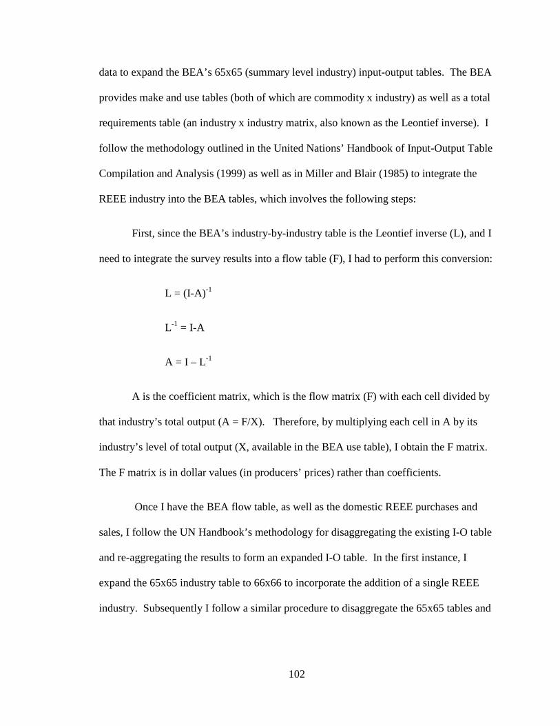
102
data to expand the BEA’s 65x65 (summary level industry) input-output tables. The BEA
provides make and use tables (both of which are commodity x industry) as well as a total
requirements table (an industry x industry matrix, also known as the Leontief inverse). I
follow the methodology outlined in the United Nations’ Handbook of Input-Output Table
Compilation and Analysis (1999) as well as in Miller and Blair (1985) to integrate the
REEE industry into the BEA tables, which involves the following steps:
First, since the BEA’s industry-by-industry table is the Leontief inverse (L), and I
need to integrate the survey results into a flow table (F), I had to perform this conversion:
L = (I-A)-1
L-1 = I-A
A = I – L-1
A is the coefficient matrix, which is the flow matrix (F) with each cell divided by
that industry’s total output (A = F/X). Therefore, by multiplying each cell in A by its
industry’s level of total output (X, available in the BEA use table), I obtain the F matrix.
The F matrix is in dollar values (in producers’ prices) rather than coefficients.
Once I have the BEA flow table, as well as the domestic REEE purchases and
sales, I follow the UN Handbook’s methodology for disaggregating the existing I-O table
and re-aggregating the results to form an expanded I-O table. In the first instance, I
expand the 65x65 industry table to 66x66 to incorporate the addition of a single REEE
industry. Subsequently I follow a similar procedure to disaggregate the 65x65 tables and

103
integrate 3 new REEE industries (RE Production and Sales, Energy Services, and Green
Building) into a 68x68 table.
The disaggregation entails dividing each of the implicated industries into the
portion which is attributable to REEE and the portion which remains as part of the
original industry. I make two assumptions when performing this aggregation. The first
is that the inputs (purchases) will be the same for both the REEE portion and the
remaining portion of the industry. So, for example, if I disaggregate the construction
industry into REEE construction and remaining construction, I assume that the
distribution of purchases is the same (for lumber, hardware, etc.). The other assumption I
make here is that the consumption pattern (sales to other industries and to final demand)
is the same between the REEE industry and the remaining industry.
To perform the disaggregation, for each industry n which is a part of REEE, I
multiply the nth column by w1 and the same nth column by w2. From one industry (one
column) I now have 2 columns with weights w1 and w2. Next I do the same for each row
n. I multiply the nth row by w1 and w2, where w1 is the weight of the industry apart from
REEE and w2 is the portion of the industry attributable to REEE. For each industry, I
determine w1 and w2 by calculating the share of the REEE sales within the total sales for
the industry. For example, if the total construction sales for our survey data (after
adjustments and scaling) equal $100,000, and the sales for the entire construction
industry within the BEA data equal $1,000,000, then w1=0.9 and w2=0.1.
Each cell in the original flow matrix, with a value of fij, is now split into four cells
as a result of this disaggregation:

104
Fij �
Disaggregation Matrix – One Industry into Two
We can also write this as F = SfS’ where f is the original flow matrix, S is the
disaggregation matrix of w’s and F is the resulting flow matrix.
Next, I aggregate all of the columns and rows with w2’s (all of the cells which
will form the new column and row of the REEE industry). I add all of the w1fnnw2 values
across the columns of the table to form the new column entries, and all of the w2fnnw1
down the rows of the table to form the new row entries. Then the w2fnnw2 will form the
new cell at the junction of the REEE column and row.
Once I perform this disaggregation and re-aggregation, I should end up with an
inter-industry flow table whose total value is the same as the total value of the original
flow table (the sum of the cells in F should equal the sum of the cells in f), since I have
not added any inputs or output to the economy, I have only reorganized the existing level
of inputs and output. Having performed this internal check, I can ensure the validity and
accuracy of the above procedure.
Now I have the new flow matrix, F, which I need to convert to a Leontief inverse
matrix and then an employment requirements table. First, I convert the flow matrix to a
w1f ijw1 w1f ijw2
w2f ijw1 w2f ijw2

105
coefficients matrix, A, by dividing each cell in each column by that industry’s total
output value. I then perform the reverse of the steps above to derive the L matrix. From
this, I can calculate output multipliers, which show the dollar value of increased
economic activity resulting from a dollar increase in final demand for the product or
service of a given industry or set of industries.
To study the effects on employment, rather than simply output, I also need to
calculate employment/output ratios. My employment and output data for our original 65
industries are extracted from the BEA.35 The employment and output data for the REEE
industry is the total employment and total output reported by all survey respondents. I
generate an employment/output ratio for each industry, and form an employment/output
vector, which I call “e.” See table 9 for the employment/output ratios of each industry in
the model.
To create the employment requirements table, E, I create a 66x66 diagonal matrix,
which I call ‘e’ (the dimensions are 66x66 since we are using 65 industries plus the
REEE industry). Each element along the diagonal of e will represent the
employment/output ratio unique to the industry in that row and column. Then, to
generate the employment requirements table I pre-multiply the Leontief inverse matrix by
the diagonal matrix of employment/output ratios as follows:
E = e(I-A) - 1
35 Gross Output by Industry and Full-Time-Equivalent Employment by Industry are available in the GDP-by-Industry data, found here: http://bea.gov/industry/gdpbyind_data.htm. We use 2006 data.

106
Where (I-A) – 1 is the Leontief inverse table (or total requirements table) and e is
the 66x66 matrix with employment/output values along with diagonal and zeros
elsewhere.
From the employment requirements table, E, I can calculate the number of full-
time- equivalent direct and indirect jobs that result from a given increase in demand. In
this case, the table shows the number of jobs created per $1 million of demand.
Incorporating 3 Distinct REEE Industries
The methodology to incorporate 3 new industries into the existing I-O tables, as
opposed to only 1, is comparable to the procedure I followed above. While this
methodology for integrating multiple industries is not explicitly introduced in the U.N.
Handbook, we can nonetheless follow the same series of steps to expand the 65x65 BEA
table into a 68x68 table.
I decompose the REEE survey responses into 3 industries: RE production and
sales; Energy Services; and Green Building. I group all of the purchases and sales by
industry into these three categories, and adjust the results as above, taking into
consideration inflation, growth, and the national scale of the industry. Of the total
adjusted values for revenues, I find that RE production and sales make up 18%, Energy
Services make up 67%, and Green Building 15%. I also calculate employment/output
ratios for each of these three industries, based on survey data. These ratios are presented
in table 10.

107
As above, I must first decompose all of the industries within the 65x65 BEA
input-output table into the portion attributable to each of these 3 REEE industries and the
portion that remains. Now, each cell in the flow matrix (f), instead of being split into
four cells (2x2) will be split into 16 cells (4x4). This results because the disaggregation
matrix will now consist of weighting values w1, w2, w3, and w4. Now the original flow
matrix (f) will map into the new flow matrix (F) as follows:
w1fnn w1 w1 fnn w2 w1 fnn w3 w1 fnn w4
w2 fnn w1 w2 fnn w2 w2 fnn w3 w2 fnn w4
w3 fnn w1 w3 fnn w2 w3 fnn w3 w3 fnn w4
w4 fnn w1 w4 fnn w2 w4 fnn w3 w4 fnn w4
Disaggregation Matrix – One Industry into Four
As above, I use this disaggregation matrix (S) to create a new flow matrix, F,
where F = SfS’. I then aggregate all of the w2 columns and rows into an RE Production
and Sales column and row, and do the same for w3 (Energy Services) and w4 (Green
Building). I aggregate the remaining w1 columns and rows into the ‘remaining’ industry,
which is the original BEA industry without the REEE elements.
Once I have re-aggregated the values into the new flow table, I obtain a 68x68
matrix. I then once again divide each cell’s value by its industry’s total output to arrive at
the A matrix (A = F/X where X is total industry output). Then from the A matrix I derive
the Leontief inverse matrix as above, then once again form the diagonal matrix ‘e’ with
fnn �

108
employment/output values. This time the diagonal matrix will be 68x68, with the first 65
diagonal elements being the BEA employment/output ratios, and the last three diagonal
elements being the employment/output ratios I calculated from the survey responses. I
then create the 68x68 employment requirements table as follows:
E = e(I-A) - 1
Where (I-A) – 1 is the Leontief inverse table (or total requirements table) and e is
the 68x68 matrix with employment/output values along with diagonal and zeros
elsewhere.
I now have created a 66x66 input-output table with a single REEE industry and a
68x68 input-output table with three distinct new industries. In the next section I will
discuss the results of this analysis.

109
CHAPTER 6
RESULTS AND DISCUSSION
Results
In this section, I present the present the results from these alternative methods of
using the input-output model to analyze the employment effects of expanding the REEE
industry. First I present the results from integrating the survey data. I start by integrating
the survey responses as a single REEE industry, and then as three separate REEE
industries. I present each of these sets of results in turn. Next, I use the synthetic
industry approach to model the REEE industry using various specifications. Finally, I
use data from the survey to construct weights for synthetic REEE industries so that I can
more directly compare these two methods of modeling. I also perform robustness tests
for each of these methods of analysis.
Survey Integration Results
REEE Industry
I start by consolidating all of my survey results into a single REEE industry and
then integrating this industry into the existing 65x65 BEA input-output tables as
described above. Since the existing 65 industries within the BEA tables are
disaggregated and re-organized into this new expanded table, all of the employment
multipliers from the resulting employment requirements matrix will be slightly different.
I present here the employment multipliers (FTE employment per $1 million demand)
from the original BEA table as well as the expanded table. As we see in table 11, the
110
original 65 industries see a very slight change in the value of their multiplier, and the 66th
industry, REEE, is now explicitly identified.
As shown in table 11, the average total employment multiplier in the original
BEA table is 9.28 jobs per $1 million demand, while the average in the expanded table is
9.13. This difference stems almost entirely from changes in the indirect effects, which
average 3.50 in the original table and 3.37 in the expanded table. The employment
multipliers in industries which are part of the new REEE industry, such as farms (for
biomass) and electrical goods (wind, solar, and others), tend to see greater change in their
employment multiplier than industries such as social assistance or accommodation, which
nevertheless see a change but a much smaller one.
Also in table 11, we see that the REEE industry has an employment multiplier of
7.29 jobs per $1 million, of which 5.24 are the direct jobs and 2.06 are the indirect jobs.
These multipliers are below the average on all levels – direct, indirect, and total. The
lower direct multiplier indicates that REEE is more capital-intensive than the average
industry. The lower indirect multiplier indicates either that the REEE industry has a less
significant supply chain than the average industry (there are fewer inter-industry
transactions) or that the industries with which REEE transacts also tend to be more
capital-intensive (or both factors may come into play). The result is a lower-than-average
total multiplier. The results are also lower than the median values, which are 8.60 in the
original table and 8.34 in the expanded table.
The REEE industry multiplier of 7.29 compares with industries such as electrical
equipment (7.41), primary metal manufacturing (7.08), management of companies (6.98),

111
and publishing industries (7.52). The lowest employment multipliers are found in oil and
gas extraction (2.18) and utilities (2.79), while the highest are found in social assistance
(20.9) and food services and drinking places (19.08). Below in the discussion section we
will evaluate possible reasons why the REEE multiplier is lower than average.
Three Distinct REEE Industries
Next I group the survey responses into three separate categories: RE Production
and Sales; Energy Services; and Green Building (which also includes retrofitting). As we
observed with the above integration, we will once again see the values of the original
employment multipliers change slightly in the expanded tables, with greater change in
those industries that are more heavily implicated in the REEE industries. The difference
in employment multipliers between the two expanded tables is, however, negligible. In
table 12 I present employment multipliers for the original and both expanded tables,
where the expanded tables are 66x66 and 68x68. For the sake of clarity, I only present
the total multipliers in table 12.
We see from table 12 above that an interesting result emerges. The employment
multipliers for RE Production & Sales and for Energy Services are 6.96 and 6.73,
respectively. Both of these are lower than the average total multiplier of 9.09. However
the Green Building industry has a higher-than-average multiplier of 10.17. This latter
multiplier compares with industries such as construction (10.58) and Federal government
enterprises (also 10.58). Below I will turn to reasons for the differences between various

112
REEE multipliers. But first I examine the results of using the synthetic industry approach
to measure REEE employment impacts.
Synthetic Industry Results
As previously discussed, the synthetic industry approach consists of determining
the components of an industry which is not part of the existing I-O tables, assigning
weights to those components, and then forming a vector of change in final demand. This
vector of change in demand is then multiplied by the employment requirements matrix to
estimate the employment impacts. Using this methodology, I have estimated various
specifications for the REEE industry as a whole, as well as components of that industry
such as wind, solar, and biomass.
Before turning to the results, I present the weights and components of these
various industries and specifications. For these estimates I use the 2006 65-industry BEA
input-output tables, which I have converted into an employment requirements matrix.
The employment multipliers from this table are presented in the previous section in table
11.
Industries and Weights
The “Green Program” is a composition of various renewable energy and energy
efficiency industries as described by Pollin, Heintz and Garrett-Peltier (2009). The
renewable energy industries include wind, solar, and biomass, while the energy efficiency
industries include building weatherization, mass transit and freight rail, and smart grid
development. My co-authors and I first assign weights to each component industry and
then aggregate these industries into the “Green Program” which is a weighted average of

113
these six REEE areas. The resulting industries and weights for the Green Program, as
well as the industries that comprise it, are in table 13.36
Using the industries and weights in table 13, I constructed vectors of change in
final demand and pre-multiplied them by the 65x65 employment requirements matrix, as
described in the methodology section above. As a result, I obtained employment
multipliers (direct and indirect) for the REEE industries listed in table 13. The
employment multipliers are shown in table 14.
As we see from the results in table 14, the synthetic industry approach produces
results that range from 8.79 (Smart Grid) to 12.83 (mass transportation and freight rail)
for total employment multipliers. The Green Program is a weighted average of the six
other industries in the table, and this is the industry with which we can most directly
compare the employment estimates we found using the integrated survey data approach.
Here the Green Program results in an employment multiplier of 10.59 direct plus indirect
jobs per $1 million demand. This is higher than my integrated survey result of 7.29. I
will discuss reasons for this difference below. Before that, however, I present the results
of one other method of estimation.
Using Synthetic Industry Approach with Survey Data
My first set of estimates involved integrating survey data into the I-O tables and
creating new industries. The second set of estimates used the existing I-O tables, without
36 Note that the weights presented here are slightly different from the weights presented in Pollin, Heintz, and Garrett-Peltier (2009). The weights used in that paper were based on a more detailed 440-industry breakdown while here we are analyzing the more aggregated tables at the 65-industry level.

114
reorganization, to estimate the effects of a demand stimulus using the synthetic industry
approach. In this final round of estimation, I create a hybrid of the previous two
methods. Here, I use sales data from the firms in our REEE survey to form a vector of
final demand, and apply that to the existing (65x65) employment requirements matrix.
The REEE sales data serves as my proxy for final demand for REEE products and
services. That is, here I form a synthetic industry where the industries and weights derive
from my survey data. First I present the weights and then I turn to the resulting
employment estimates. Once again, in this table I suppress the industries which have
zero values in all categories.
Using the industries and weights in table 15, I generate final demand vectors and
apply them to the existing (unmodified 65x65) employment requirements table. This
results in the employment estimates shown in table 16.
Interestingly, when I use this approach the order of the size of employment
multipliers changes from when I use the integrated survey data. Here, Energy Services
now has the highest multiplier, with 10.09 total jobs per $1 million, followed by Green
Building at 9.15 and RE Production and Sales with 8.81. With the integrated approach,
Green Building had the highest multiplier (10.17) followed by RE Production and Sales
(6.96) and finally Energy Services (6.73). Thus the values with the hybrid approach are
not only higher in all categories, but also affect the ordering of the industries in terms of
the size of the multiplier. My REEE category has a total multiplier of 9.72 using this
hybrid approach compared to 6.56 using the integrated approach. We can compare this to
the Green Program in the synthetic industry approach, which has a total multiplier of
10.59. Thus the hybrid approach yields a result between the values obtained using the

115
other two approaches. Before turning to a discussion of these various sets of results, I
first perform a series of robust tests.
Robustness Tests
Survey Integration Robustness Tests
The input-output model is a snapshot of the economy at a point in time. It does
not consist of a distribution or expected values, outcomes that we might test through
typical robustness checks such as standard deviations or other tests of statistical
dispersion. In order to check the robustness of the results of our survey data integration,
therefore, I can perform simple tests throughout the process to ensure that I have
correctly manipulated the matrices, and I can compare my results to other methods of
estimating employment, as well as to estimates from the original I-O tables, to check
whether my results are reasonable.
When integrating the survey data, I start with the original flow table from the
BEA, which is a 65x65 table that shows flows (in dollars) of goods and services between
industries. I can add the total dollar value of all of the cells in the matrix and use this as a
check. When I integrate the survey data, I disaggregate, reorganize, and re-aggregate the
original flow table (f) into a new expanded flow table (F). Because this exercise is
simply a reorganization of the data, and I am not adding or subtracting any transactions
from the economy, the elements of f should equal the elements of F, meaning that the
total dollar value of all inter-industry transactions should be the same in the original and
expanded tables. I performed this check both with the 66x66 flow matrix as well as with
116
the 68x68 matrix, and in both cases the elements added up to the same value as the
elements in the original 65x65 flow matrix.
The other check I can perform that could serve as a robustness test is to compare
the employment multipliers from the expanded employment requirements matrix to those
obtained using the original ER matrix. I presented these results in tables 11 and 12. If
the integration of the data and expansion of the tables had been done incorrectly, we
would see large discrepancies between the original and expanded table multipliers.
However, as shown in those tables, the differences between the multipliers are small, and
result mainly from changes in the indirect effects. Thus I can be reasonably confident
that the integration was performed correctly and my results are robust.
Synthetic Industry Specification Tests
The synthetic industry approach does not involve expanding the I-O tables but
only multiplying the existing employment requirements table by a vector of final
demand. Therefore in order to test the robustness of our results I can alter the
specification of the final demand vector to see how sensitive the outcome is to the choice
of specification. If a small change in specification produces a large change in the
employment multiplier, then the estimates are not likely to be robust. However if a
significant change in the specification results in minimal change in the multiplier, then I
can be assured that the results are robust. In Chapter 3 I performed one such check using
the example of the wind industry. Here I will perform a series of specification tests for
the Green Program as well as for the REEE industry. The prior was defined by Pollin,
Heintz and Garrett-Peltier (2009) while the latter appears here both in the integrated

117
survey approach and the hybrid approach. I will modify the REEE industry as presented
in the hybrid approach, which consists of creating a vector of final demand from the sales
data from firms in our survey.
In table 17 we see that a large change in the specification of the green program
results in a much smaller change in the employment multiplier. In the original
specification of the green program, manufacturing industries had a 20.7% share while
non-manufacturing (largely construction) made up the other 79.3%. In each alternative
specification, I increase or decrease the shares of manufacturing versus non-
manufacturing by 10, 20, and 30 percentage points. A 10 percentage point change in
shares results in an employment multiplier that is 2.83 percent different from the original
(smaller as the share of manufacturing increases, larger as this share decreases). A 20
percentage point change in specification results is a 5.66 percent change in multiplier,
and a 30 percentage change results in a multiplier that changes by 8.49 percent. These
results show that my estimation results are not very sensitive to the choice of
specification, and that the employment multipliers for the Green Program can be
considered robust. These results hold because the various industries that makes up the
Green Program – both in services and in manufacturing – have employment multiplier
values that are not highly varied. If the green program had included industries such as
extraction activities (on the low end of the employment multiplier spectrum) or certain
services such as social services (on the high end of the spectrum), the results would have
been sensitive to the choice of specification. However, all of the industries which
comprise the green program have a range of employment multipliers that is relatively
compressed, and therefore even a large change in how these industries are weighted in

118
the overall composition of the program results in only a small change in the green
program employment multiplier.
I perform the same exercise with our specification of the REEE industry. Here
the original weights are derived from the sales data of firms in our survey, as presented in
Table 18. Surprisingly, even though the composition of the individual industries differs
between the Green Program and the REEE industry (a point to which I will return below),
the shares of manufacturing and non-manufacturing industries are quite similar between
the Green Program and the REEE industry, with manufacturing accounting for 20.7
percent of the original specification of the Green Program and 21.6 percent in the original
REEE specification.
As in the previous exercise, I find that here the total employment multiplier is not
sensitive to the choice of specification. A ten percentage point change in the share of
manufacturing versus non-manufacturing results in only a 1.57 percent change in the
multiplier. A change as large as 30 percentage points, so that manufacturing makes up a
51.6 percent share instead of the original 21.6 percent, results in an employment
multiplier that is only 4.72 percent different from the original (9.26 instead of 9.72).
Once again, this result obtains because the various manufacturing and services industries
that make up the REEE have a relatively compressed range of employment multiplier
values, and do not include some of the more extreme employment multiplier values found
in industries such as extraction (extremely low) or social services (extremely high).
Therefore a large change in the composition of the industries comprising the REEE
industry results in only a small change to the employment multiplier. Thus here as well I
can consider my results robust as they are not sensitive to the choice of specification.

119
Now that I have shown the robustness of my results both using the integrated method and
the synthetic industry approach, I turn to a discussion of the results of my analyses.
Discussion
Comparison of Results from Alternative Methods
In the previous sections I presented results for employment impact analysis of the
REEE industry by first integrating survey data, then creating synthetic industries, and
finally using a hybrid strategy that incorporates data from the first with the methodology
of the second. In table 19 I present a comparison of these various results so that I may
then discuss my findings and possible sources for variation in the outcomes. I include the
REEE industry from the expanded 66x66 I-O method, the three industries from the 68x68
expanded matrix, two industries using the synthetic approach (the Green Program, which
we can compare to REEE; and Building Weatherization, which we can compare to Green
Building), and well as the REEE industry and 3 sub-components using the hybrid
approach.
As we see from table 19, various methods and definitions for estimating
employment impacts for the REEE industry lead to a range of results, with a low of 6.73
in Energy Services using the integrated survey approach, and a high of 10.69 in Building
Weatherization using the synthetic industry approach. The three overall REEE categories
with similar definitions are REEE (66x66), Green Program (Synthetic), and REEE
(Hybrid). These have total multipliers of 7.29, 10.59, and 9.72, respectively. The other
category that is similar across methods is Green Building. The survey method leads to a

120
Green Building multiplier of 10.17, while Building Weatherization (synthetic) is 10.69
and Green Building (hybrid) is 9.15. Thus the result of the REEE industry is much more
sensitive to the choice of method of analysis, while Green Building is relatively stable
across these three methods. This is an expected outcome, since Green Building mainly
consists of the construction industry, while REEE is composed of many different
industries, each with its own set of multipliers. Below I discuss reasons for differences in
these employment estimates. Before doing so, however, I compare my estimates to those
published in other studies.
Comparing Results to Other Studies
Here I compare my results to those obtained in previous research, namely the
studies I reviewed in Chapter 2. I limit my comparison to studies which used input-
output models and developed employment multipliers. In table 20 I compile the results
of some of these studies.
From table 20, we see that the three methods of estimation employed here yield
results that fall within the range of results found in other studies. Sterzinger (2006) and
Singh and Fehrs (2001) present only direct effects for renewable technologies, and thus
their estimates fall at the bottom end of the range (5.3 jobs/$1 million and 5.7 jobs/$1
million, respectively). These estimates are followed by studies that report both direct and
indirect employment. In that category, Bezdek (2009) estimates 8.6 jobs/$1 million for
both energy efficiency and renewables. Estimates by Laitner (2009) of 15.9 jobs/$1
million also include both direct and indirect jobs, but are restricted to energy efficiency.
The top end of the range is 26.8 jobs per $1 million, estimated by Roland-Holst (2008).

121
This estimate captures direct, indirect, and induced effects, but is restricted to energy
efficiency. My own estimates include both direct and indirect effects, and both
renewable energy and energy efficiency. In comparison to the results in these other
studies, my estimates are higher than those which include only direct effects, and lower
than those which include only efficiency but not renewable energy.
Turning to estimates that capture both RE and EE, we see that Pollin et al.
estimate 16.7 jobs per $1 million in REEE, including direct, indirect, and induced effects.
This is not immediately comparable with my results here, however, since I have not
modeled induced effects. However, the induced effect modeled by Pollin et al is 40% of
the direct plus indirect effects, therefore I can calculate that their direct plus indirect
effects (without induced) would be 11.93 jobs per $1 million demand. This study, along
with Bezdek (2009), are the only studies which incorporate both renewables and energy
efficiency, and that estimate direct plus indirect effects. The estimate in Bezdek (2009)
is 8.61 jobs per $1 million of investments in REEE. This falls right in the middle of our
own estimates, while the direct plus indirect effects from Pollin et al (2009) are only
slightly larger than the estimates developed in this dissertation. Thus I am confident that
my methodology and results are both internally and externally robust.
Reasons for Differences between Methods
All of the employment estimates presented here are derived from an input-output
model using an employment requirements matrix. Aside from differences resulting
strictly from the inherent methodological differences (discussed below), any other
difference in the estimates can be traced to three sources: output multipliers (which show

122
the effects of industry output and inter-industry transactions), employment/output ratios
(which convert inter-industry transactions into an employment requirements matrix), and
differences in final demand. The differences in output multipliers and
employment/output (E/O) ratios apply to all three strategies. The differences in final
demand are relevant only for the synthetic and hybrid approaches, since these rely on
changing the vector of final demand. I discuss each of these sources of variation in turn,
and end the discussion with the differences due strictly to methodology.
Differences in Output and Employment Multipliers
Within any input-output model, each industry will have its own unique set of
interactions with other industries the economy, its own production function. Some
industries will buy inputs from many others, while other industries will buy few.
Likewise, the output that a given industry produces may be used by itself, by other
industries, or by various sources of final demand, and each industry will have its own
unique set of output (and sales) relationships. The Leontief Inverse matrix captures the
inter-industry transactions and allows us to calculate output multipliers for each industry.
An output multiplier shows how many dollars of total output are produced economy-wide
in order to satisfy one dollar of demand for an industry’s product. If we take the example
of the farming industry, in order to satisfy a consumer’s demand for $1 of output (say,
wheat), the farm industry must produce $1 worth of wheat, plus some of its own products
that go into producing wheat (such as seed) and must use the output of other industries
(such as farm equipment from the machinery industry and fertilizer from the chemical
industry). Therefore $1 in final demand creates more than $1 of total output. The
Leontief Inverse matrix shows how much output, by industry, is generated by the
123
additional demand. By comparing output multipliers, we can see the extent to which
industries rely more or less heavily on the output of other industries, thus how much
additional economic activity is generated by increased demand for each industry’s
products. The output multipliers for the three versions of my Leontief Inverse matrix
(65-, 66-, and 68-industry) are presented in table 21.
Continuing with the example above, we see that for the farm industry, in order to
meet $1 of final demand, there are about $2.36 of output economy-wide, including $1.20
in the farm industry itself and about $1.17 in other industries which supply it. Turning
now to REEE, we see that in the 66-industry expanded table, $1.47 of output is produced
economy-wide for every $1 demand for REEE goods and services. We see that most of
this increased output comes from industries which supply REEE, rather than the REEE
industry using its own output as inputs. The output multiplier of 1.47 is lower than the
average multiplier across all industries of 1.93. Since the output multiplier table isolates
input-output relationships before we introduce employment, this result shows that the
lower-than-average employment multipliers (previously discussed) stem at least in part
from lower-than-average input-output relationships. When we decompose the REEE into
three distinct industries and create a 68x68 table, the direct output multiplier for these
industries is once again close to one, below the average direct multiplier of 1.10. Here,
however, we see that RE Production & Sales and Green Building have higher-than-
average indirect multipliers, resulting in total output multipliers that are very close to the
average across all industries. Energy Services has lower indirect and total output
multipliers, and as a result falls below the industry average. Thus this sub-component of
the REEE industry may be driving the lower-than-average output multiplier of the REEE
124
industry in the 66-industry table. Therefore the low employment multipliers for REEE as
a whole as well as for Energy Services in particular are driven at least in part by input-
output relationships. RE Production & Sales, however, has a lower-than-average
employment multiplier but an average output multiplier, therefore the low employment
multiplier must be attributable to another cause, namely, a low employment/output ratio.
Differences in Employment/Output Ratios
The ratio of employment to output is a measure of labor intensity. It is a ratio of
the number of full-time-equivalent jobs per $1 million in gross output for each industry in
the matrix. Lower E/O ratios imply lower labor intensity, and vice versa. As described
earlier, the E/O ratio for each industry is multiplied through the Leontief inverse matrix
in order to create an employment requirements matrix. If two industries have similar
output multipliers but different employment multipliers, then this difference is
attributable to differences in E/O ratios.
As an example, the RE Production & Sales industry has an output multiplier that
is close to the average, but an employment multiplier that is below average. We know,
therefore, that this discrepancy stems from a low E/O ratio, implying that RE Production
& Sales is less labor-intensive than the average industry. Below I compare the total
output multipliers, employment multipliers, and employment/output ratios for each of our
REEE categories as well as the industry averages. Note that the employment multiplier is
not the product of the output multiplier and the E/O ratio. The employment multiplier
accounts for the E/O ratios in all of the industries supplying inputs to and buying output
from the industry in question.

125
We see from table 22 that REEE, RE Production & Sales, and Energy Services all
have lower-than average employment multipliers. This table shows that the source of the
lower multiplier is different in all three cases. In the case of the combined REEE
industry, both a lower output multiplier and a lower E/O ratio contribute to the lower
employment multiplier. In RE Production & Sales, the lower employment multiplier is
entirely attributable to a lower E/O ratio, and in Energy Services it is entirely attributable
to a lower output multiplier. Green Building stands alone, in that it has a higher-than-
average employment multiplier, which we see here is the result of a higher-than-average
E/O ratio. These results indicate that REEE and RE Production & Sales are more capital-
intensive than the average industry while Green Building is more labor-intensive. Energy
Services has average labor intensity but has a lower level of inter-industry transactions.
The E/O ratios, which are presented above and used in my integrated I-O analysis,
derive from data collected by firms in our survey, which is only a small sample of all of
the firms in the REEE industry. It is quite possible that the firms in our survey are not
representative of the entire population of REEE firms, and that the E/O ratios based on
our survey respondents are lower than the true population value of the economy-wide
REEE E/O ratio. If indeed the true E/O ratio is higher, then of course the employment
multiplier would itself also be higher. In three of the four cases presented above, the E/O
ratio is a driver in the employment multipliers being above or below the mean. Below, I
present the results of a counterfactual test: What if the E/O ratio was the same as the
industry average? I re-create the employment requirements matrix for the 66- and 68-
industry tables and present the outcomes in table 23.

126
As we see from table 23, when I use the average E/O ratios to create the
employment requirements matrix, the employment multipliers for REEE and RE
Production & Sales both rise, while those for Energy Services and Green Building both
fall. This is of course the anticipated result, since the prior two categories had lower-
than-average E/O ratios and the latter had higher-than average. The resulting differences
in employment multipliers between each of these industries and the industry average are
then attributable to differences in inter-industry transactions, which are captured by the
output multipliers. RE Production & Sales now has an average-level employment
multiplier, and Green Building remains above-average. REEE as a whole, however, as
well as its component industry Energy Services, both still have below-average
employment multipliers which are therefore attributable to below-average inter-industry
transactions.
In order to compare the results across different methods of analysis, I can conduct
a similar exercise to decompose the synthetic industry multipliers into output multipliers
and E/O ratios, and compare those with the above results which use the integrated survey
data. The synthetic industry approach uses a demand stimulus to estimate employment
effects. I use the same composition and weights to form a weighted average E/O ratio for
each of the synthetic industries. In table 24 I present the results for the Green Program
and for Building Weatherization, the two synthetic industries most directly comparable
with the REEE results presented above.
Table 24 shows that the Green Program (synthetic) has an above-average output
multiplier and E/O ratio, resulting in an above-average employment multiplier. We
contrast this with the REEE industry (integrated) which has below-average values in both

127
of these areas. Thus REEE as modeled has a lower employment multiplier than the
Green Program due to both lower inter-industry transactions and lower labor intensity.
Building weatherization in the synthetic approach also has a higher-than-average
output multiplier and E/O ratio, and is higher than the integrated Green Building industry
in both categories. The slight difference between the total employment multipliers in
Building Weatherization and Green Building is therefore also attributable to variations in
both inter-industry transactions and labor intensity, though the differences in both of
these categories are relatively small.
Differences in Final Demand
The employment estimates may vary between different specifications for the
REEE industry for an additional reason, which is differences in the composition of final
demand. This applies mainly to the synthetic and hybrid approaches, which multiply a
vector of change in final demand to the current employment requirements matrix to
estimate employment impacts of expanding the REEE industry. The hybrid approach,
however, can also shed light on the results from the integrated approach. The two
sources of variation in the integrated approach are the E/O ratio and the output
multipliers, which show the extent of inter-industry transactions. If we look at sales by
the REEE firms in our survey, this gives a partial indication of inter-industry transactions
(outputs, not inputs). It is this sales vector that I use in the hybrid approach. Thus if we
compare the survey sales vector to the vector of demand used for the Green Program or
Building Weatherization, we will see differences in industrial composition that will allow
us further to isolate the source of the variation. In tables 13 and 15, I show the

128
composition of synthetic industries and the survey demand stimulus, respectively. In
table 25 I present the Green Program and REEE Industry from those tables, and highlight
the industries in which the share of demand varies by more than five percentage points
between the Green Program and REEE. I suppress the rows that have zero values for
both REEE industries.
As we see from table 25, there are a few significant differences in the industrial
composition of the REEE survey sales as compared to the Green Program. The three
biggest differences are found in Construction; Miscellaneous professional, scientific, and
technical services; and Waste management. In the case of construction, the Green
Program weights this category much more heavily – it accounts for just over half of all
Green Program industrial activity. In the case of the professional/scientific/technical
services and waste management, these are represented much more heavily in the survey
responses than in the synthetic Green Program. Other notable categories that have a
more significant presence in the survey sample are non-metallic mineral products,
miscellaneous manufacturing, and education, while transit and ground passenger
transportation make up a greater share of the Green Program demand. These differences
are all greater than five percentage points, and may have a significant impact in
determining the value of output multipliers for these industries, which, as we see above,
differ from each other. My survey may have over-sampled advocacy and education
groups, or perhaps the Green Program should explicitly include this industry in its
composition. Likewise, in all of these categories where significant differences are
present, it may be the case that the survey sample is not representative, or it could be that
the Green Program is not properly specified. The above information does not tell us

129
which is the case. It does, however, offer some guidance as to how I might redefine the
synthetic industries or improve the sampling and survey responses in future surveys.
Inherent Methodological Differences
As discussed in chapter three, the synthetic industry approach and integrated
industry approach differ in one major way – the synthetic approach treats changes in
demand for REEE products and services as an exogenous shock, while the integrated
approach endogenizes this industry and therefore captures linkages in both directions.
This difference may be an important factor driving the differences in results between the
synthetic and integrated approaches. In the synthetic approach, the REEE industry
(“Green Program”) is treated as a consumer with a unique set of final demands (metal,
hardware, turbines, and so on). In the integrated approach, the REEE industry consumes
inputs from other industries but also enters into the production function of other
industries as it supplies output to meet intermediate demands.
If, however, the REEE industry is an insignificant provider of goods and services
to other industries (in other words, if REEE serves mainly final demands but not
intermediate demands), then the results from the two approaches could be quite similar,
or the multipliers from the integrated approach could even be lower than those of the
synthetic approach. For example, if REEE is small relative to other industries, then the
level of inter-industry demand for REEE may be minimal in relation to demand for the
output of other industries. Another possibility is that REEE products are treated as
capital improvements or investment goods, and are not part of the ‘flow’ of goods and

130
services that is captured within the basic I-O framework.37 If this is the case, the REEE
industry may indeed function more as a consumer, as it buys inputs from multiple
industries but does not itself enter into the production function of those (or other)
industries. It is quite possible that one or both of these factors – the size of the industry
and the treatment of its products as capital – could explain the low level of inter-industry
transactions in the integrated approach, as captured by the below-average output
multiplier discussed above. This lower output multiplier drives the lower employment
multiplier. This lower level of inter-industry transactions would manifest itself only in
the integrated approach, and not the synthetic industry approach, and therefore this could
be an important factor in explaining the lower REEE employment effects obtained with
the integrated approach.
Which Estimation Method Is More Accurate or Appropriate?
As we see from the results above, there are some non-negligible differences in
modeling REEE employment depending on which method of analysis we use. Which
method is more accurate or appropriate? It is not immediately clear that one approach is
superior to the other. The integrated survey method is an analytically sound approach,
but is potentially fraught with errors due to the size, scope, and reliability of our survey
responses. The sample of REEE firms, though nationwide and representing various parts
37 Dynamic input-output models introduce both a time dimension and investments in capital stock. These models build upon the static model used here by introducing a separate capital coefficients matrix in which each entry represents the stock of capital of industry i which is used by industry j over time period t. For more on this issue, see (Richardson, 1972) or (Leontief, 1986).

131
of the REEE industry, may in fact be unrepresentative of the true population of REEE
firms. Our survey responses may over-represent some industries and under-represent
others. There may also be reporting errors by the respondents that lower the quality of
the data. We may have captured too many small firms or newer firms, since the industry
is growing rapidly and since some larger firms were unwilling to report their financial
data. Finally, the survey results were adjusted for inflation, growth, and scale before
being integrated and there may be discrepancies resulting from these adjustments. The
synthetic industry approach may therefore be more accurate or reliable, since it involves
using data in the existing BEA input-output tables, which are created from surveys of
millions of firms and are therefore much more representative of the population of U.S.
businesses.
The integrated survey approach is, however, superior to the synthetic industry
approach in some ways. The synthetic approach uses only a demand stimulus, capturing
one side of the effects of the REEE industry. The integrated approach captures not only
the sales (output) of the REEE firms but also integrates data on their inputs, thus
generating a more complete picture of the economic impacts and inter-industry
transactions of which REEE plays a part.
The hybrid approach, finally, is essentially just a different and potentially better
way to compose the final demand vector, but suffers from the same problem of not
capturing intermediate demand of the REEE industry. Since it is based on survey data, it
could also suffer from the problems noted above that are inherent to smaller-scale
surveys.

132
Thus all of these approaches offer insights into modeling employment in the
REEE, but none is superior in all ways to others. The ideal, of course, would be that the
U.S. Department of Commerce creates NAICS codes for the REEE sector, and that the
Census Bureau collects and identifies this sector as part of their Economic Census and
other business surveys. Until then, we can use one or more of the approaches presented
here to estimate the employment impacts of investment in renewable energy and energy
efficiency.
Policy Implications of Alternative Approaches
One major objective of estimating employment effects of various energy
investments is to contribute to the public debate and policy discussions on this topic.
Government policy can support the expansion of REEE through a variety of mechanisms,
including tax credits and rebates, standards or mandates, direct public procurement,
education and advocacy programs, and so forth. In order to make informed decisions
about whether or not to support clean energy programs, policy makers will consider both
the environmental and economic effects of energy policy, as well as the specific impacts
on their own constituency. Employment is of particular concern to policy makers (as
noted by Berck and Hoffman (2002)) and therefore a comprehensive assessment of
employment impacts, which considers both the job losses as well as job gains of REEE
investments, is of critical importance to political decision-makers.
Above I presented the results of various methods for analyzing REEE
investments. I estimated employment multipliers in the REEE industry using the
integrated approach and in the Green Program using the synthetic industry approach. To

133
be relevant for policy applications, we must also consider the employment multipliers in
fossil fuels, the industries that will lose jobs as we transition to a more energy-efficient
system with a greater share of power produced by renewable energy.
In table 26 I show employment multipliers for various fossil fuel and REEE
industries based on my two primary methods of analysis. This table shows that by any
specification and method of estimating the REEE industry, the employment multiplier is
greater than in any fossil fuel industry, implying that a dollar per dollar shift from fossil
fuel spending to REEE spending will create a net positive number of jobs. The direct
employment effects for the three REEE specifications range from a low of 5.24 to a high
of 6.40, whereas the greatest direct effect in fossil fuels is found in mining (such as for
coal), with a direct effect of 3.24. The total (direct plus indirect) effects in REEE range
from 7.29 to 10.59, whereas in fossil fuels the range of total effects is from 2.26 to 5.74.
Thus even the most labor-intensive fossil fuel industry (support activities for mining) still
creates fewer jobs per dollar than the least labor-intensive specification of REEE. Thus
an economy-wide shift to renewable energy and energy efficiency will create more jobs
than it destroys.

134
CHAPTER 7
CONCLUSION
Chapter Summary
In this dissertation I first presented background statistics on energy use and
emissions within the U.S., and situated my work within the broader context of climate
change policy. We saw that the U.S. currently relies mainly on fossil fuels as an energy
source, while renewables make up less than eight percent of total energy consumption.
Energy intensity is declining at a rate of only two percent per year while GDP is rising at
a faster rate, resulting in projected increases in energy demands, including increases in
fossil fuel consumption which will contribute to rising carbon emissions. Under a
business-as-usual scenario, renewable energy and energy efficiency will grow only
slightly over the next few decades, far too slowly to be an effective response to climate
change pressures. However, even with currently available technologies, many
opportunities exist to increase our energy efficiency as well as our use of renewables.
Together, REEE can contribute nearly half of the carbon emissions reductions needed to
meet necessary abatement levels. The other half can be achieved through behavioral
change which conserves energy, through strategies such as reforestation or otherwise
increasing carbon sinks, and according to some scenarios, through the use of carbon
capture and sequestration as well as nuclear power.
In chapter two I reviewed the studies of the economic impacts of REEE
investments. While these investments are necessary to meet climate policy goals, it is
also vital to understand the economic and especially the employment impacts. The

135
studies I reviewed in chapter two take a variety of approaches to address this question.
Many are based on an input-output framework while others use non-modeling techniques
such as case studies. Within the modeled approaches, I find that the input-output model
is used in two ways. Some, such as Pollin and Garrett-Peltier (2009), use the I-O model
to estimate the number of jobs created by a given level of REEE investment. Others,
such as Laitner (2009), concentrate on the effects of energy efficiency investments,
estimate the cost savings that can be achieved through EE, then use the I-O model to
estimate the jobs that result from these cost savings. Finally, other researchers such as
Singh and Fehrs (2001) conduct interviews to estimate the number of jobs per level of
energy output (jobs/MW) at certain renewable energy manufacturing firms. The studies
presented in chapter two represent a range of methodologies, yet they come to a central
conclusion, which is that investments in renewable energy and/or energy efficiency will
have positive impacts on employment, even after considering job losses in fossil fuels.
In chapter three I describe the input-output model in detail and discuss the current
limitations of using the I-O model to study REEE, an industry which is not identified in
the I-O tables. Researchers have attempted to overcome this limitation in a number of
ways. Pollin and Garrett-Peltier use a ‘synthetic industry’ approach which consists of
identifying the components of REEE technologies (both manufactured goods and
services), assigning weights (cost shares) to those components and then creating a vector
of final demand. We can then apply this vector to the existing I-O tables and simulate the
effects of increased demand for REEE goods and services. I perform this same analysis
here, and also present a method which can be used to test for the robustness of the results.

136
The I-O model can be expanded to include the REEE industry if we have
sufficient data on REEE firms. I undertake a survey to collect such data and present my
survey methods and results in chapter four. I compiled a sample of 1,000 firms
nationwide, sent nearly 500 questionnaires to firms, and received just over 100 complete
and useable responses. These responses came from a variety of REEE businesses,
including wind and solar technology manufacture and distribution, construction and
design companies engaged in green building, and a variety of energy service companies
such as energy auditors and education organizations.
In chapter five I present the methodology for integrating this data into the I-O
tables. The methodology was developed by other authors, but to my knowledge no one
has yet applied it to the renewable energy and energy efficiency industry. I perform two
levels of integration. First, I integrate the full set of survey results into one REEE
industry. And secondly I divide the survey results into three groups and separately
integrate industries which I call “RE Production and Sales,” “Energy Services,” and
“Green Building.” The methodology is quite similar for these two integration exercises,
and I test my analysis and results for accuracy.
I present the results of these alternative methods in chapter six, which also
contains a discussion of the results, robustness tests, and comparison of the results to
previously published estimates. I find that REEE generates between 6.56 and 10.59 jobs
(direct plus indirect) per $1 million investment depending on the method of analysis. The
low end is the result of the survey integration method and the high end is the result of the
synthetic industry approach. I decompose these results into differences in output
multipliers (inter-industry relationships), employment/output ratios (labor intensity), and

137
composition of final demand. I find that all three of these factors will affect the value of
the employment multiplier, and I discuss reasons for the discrepancies. I determine that
neither approach is superior in all capacities to the other. The survey approach has the
advantage of using actual data but could suffer from an unrepresentative sample or
reporting errors. The synthetic industry approach has the disadvantage of only
considering the output relationships (not inputs) and using industry averages which might
not always be a good proxy for REEE firms, however it has the advantage of being based
on actual data from a much larger number of firms than our survey.
Contributions of this Dissertation
This dissertation has contributed to the literature on the employment impacts of
renewable energy and energy efficiency in a number of ways. First, I have provided a
review of various studies and methods used to address this question. Since this literature
is growing so rapidly, a review of this type has not heretofore been completed, and this
dissertation will advance our understanding of the advantages, drawbacks, and
comparability of using alternative modeled and non-modeled approaches.
More importantly, in this dissertation I expand upon current methods of using
input-output analysis to address REEE employment. Due to data limitations, researchers
have until now been constrained in their ability to use the I-O model to study the REEE
industry, and the authors that collect primary data to analyze REEE employment
generally have very small samples and present only case studies from which we can not
necessarily draw macroeconomic implications. Here I overcome this data constraint in
two ways. First I develop the ‘synthetic industry’ approach used by Pollin, Garrett-

138
Peltier, and others (Pollin, et al. 2008), (Pollin, Heintz, & Garrett-Peltier, 2009), (Pollin
& Garrett-Peltier, 2009). I also present a robustness test that can be used for this
approach. Secondly I collect data from REEE firms throughout the U.S. and integrate
this data into the input-output accounts. Not only does the new data set contribute to this
research area, but to my knowledge, this is the first time this methodology has been used
to examine the economy-wide impacts of the REEE industry. The results of these
alternative research methods substantiate the results previously obtained by others,
namely that investments in renewable energy and energy efficiency will have positive
employment impacts, even after accounting for job losses in fossil fuel industries.
Policy Implications
These contributions are politically both timely and relevant. With increasing
attention to the impacts of climate change on our environment and our economy,
scientists and economists are studying the ramifications of both action and inaction.
Studies have shown that energy efficiency and renewable energy can play a significant
role in abating carbon emissions. In order to drastically increase our carbon productivity
we need both public and private investment in renewable energy and energy efficiency.
The public sector can use market and regulatory mechanisms to speed the diffusion of
REEE technologies and slow the use of fossil fuels. These mechanisms can take the form
of tax credits and rebates for clean energy; public procurement of clean vehicles; energy
retrofits to public buildings; building and land-use codes; grants to organizations,
municipalities, and states to weatherize buildings and pursue other clean energy
strategies; carbon taxes or cap-and-permit systems; and a host of other regulatory and

139
financial incentives to encourage individuals and businesses to reduce their use of carbon,
increase their use of renewable energy, and become more energy efficient.
Many opportunities and technologies already exist for us to transition to a cleaner
energy economy. The research presented in this dissertation confirms the findings that a
clean energy transition will also contribute to the growth of employment. Renewable
energy and energy efficiency are more labor-intensive than carbon-based fuels, and thus
it is reasonable to assume that a transition from fossil fuels to REEE will have positive
employment impacts. This dissertation confirms this to be true, and through the use of an
input-output model as well as primary data collected from REEE firms across the U.S. we
see that the economy-wide impacts of employment from REEE investments are positive.
The magnitude of the effect depends on the type of model we use – the effects are greater
through the synthetic industry approach than the integrated survey data approach – but in
either case the outcome is the same: A transition from carbon-based energy to REEE will
be a net source of job creation.
Directions for Further Research
In this dissertation, I use a static input-output model and conduct comparative
static exercises to estimate employment effects. While this is an appropriate estimation
method in the short-run, it is not appropriate for long-run analysis of a transition to
renewable energy and efficiency. In order to study long-run effects, I would need to
incorporate both a time dimension and a capital coefficients matrix into the input-output
model. It would also be important to adjust production functions over the longer term, as
firms change their inputs of energy goods, capital, and labor in response to changes in

140
energy availability or price. Including a time dimension and capital coefficients would
create a dynamic input-output model, whereas building in additional equations and
assumptions about factor substitution and other changes in consumption and production
functions would lead to the building of a CGE model. Despite the shortcomings of CGE
models (due mainly to their multiple assumptions and lack of transparency), this may be
the most appropriate method for studying the long-run effects of REEE investments.
Another important dimension to include in future analysis is the geographical
distribution of job losses and gains resulting from a decline in fossil fuel production and
an increase in REEE. I only briefly discussed the net employment effects in chapter six –
that is, the employment gains from REEE in comparison to the loss in fossil fuel jobs.
However, in this dissertation I have only analyzed national data, and the job losses in
particular may be concentrated in certain regions of the country that are large coal
producers (e.g. Appalachia) or oil producers (e.g. the Gulf Coast). In order to target
REEE investments and training programs toward workers who would lose their jobs in
fossil-fuel industries, we would need to study the geographical distribution of those jobs.
Finally, we have seen that a shift from fossil fuels to REEE will generate a net
increase in employment and a reduction in carbon emissions, and that therefore there is a
case to be made for public support of a transition to clean energy. Further research could
evaluate the most effective means to speed the transition to REEE, including evaluating
market mechanisms such as carbon taxes or renewable energy tax credits, and regulatory
mechanisms such as building codes and renewable portfolio standards.

141
In short, the directions for further research include evaluating the political tools
that could best speed the transition to clean energy, analyzing the regional impacts of the
job gains and losses resulting from that transition, and expanding our basic input-output
model in order to study the long-run effects of a transition to REEE.
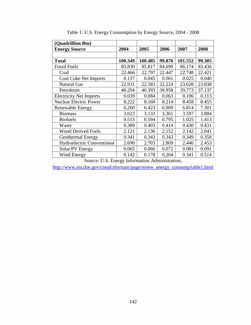
142
Table 1: U.S. Energy Consumption by Energy Source, 2004 - 2008
(Quadrillion Btu) Energy Source 2004 2005 2006 2007 2008 Total 100.349 100.485 99.876 101.552 99.305 Fossil Fuels 85.830 85.817 84.690 86.174 83.436 Coal 22.466 22.797 22.447 22.748 22.421 Coal Coke Net Imports 0.137 0.045 0.061 0.025 0.040 Natural Gas 22.931 22.583 22.224 23.628 23.838 Petroleum 40.294 40.393 39.958 39.773 37.137 Electricity Net Imports 0.039 0.084 0.063 0.106 0.113 Nuclear Electric Power 8.222 8.160 8.214 8.458 8.455 Renewable Energy 6.260 6.423 6.909 6.814 7.301 Biomass 3.023 3.133 3.361 3.597 3.884 Biofuels 0.513 0.594 0.795 1.025 1.413 Waste 0.389 0.403 0.414 0.430 0.431 Wood Derived Fuels 2.121 2.136 2.152 2.142 2.041 Geothermal Energy 0.341 0.343 0.343 0.349 0.358 Hydroelectric Conventional 2.690 2.703 2.869 2.446 2.453 Solar/PV Energy 0.065 0.066 0.072 0.081 0.091 Wind Energy 0.142 0.178 0.264 0.341 0.514
Source: U.S. Energy Information Administration, http://www.eia.doe.gov/cneaf/alternate/page/renew_energy_consump/table1.html
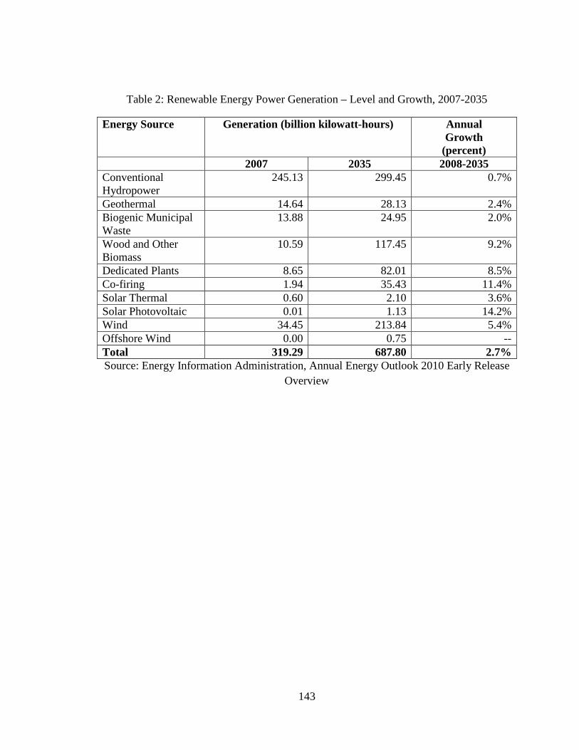
143
Table 2: Renewable Energy Power Generation – Level and Growth, 2007-2035
Energy Source Generation (billion kilowatt-hours)
Annual Growth
(percent) 2007 2035 2008-2035 Conventional Hydropower
245.13 299.45 0.7%
Geothermal 14.64 28.13 2.4% Biogenic Municipal Waste
13.88 24.95 2.0%
Wood and Other Biomass
10.59 117.45 9.2%
Dedicated Plants 8.65 82.01 8.5% Co-firing 1.94 35.43 11.4% Solar Thermal 0.60 2.10 3.6% Solar Photovoltaic 0.01 1.13 14.2% Wind 34.45 213.84 5.4% Offshore Wind 0.00 0.75 -- Total 319.29 687.80 2.7% Source: Energy Information Administration, Annual Energy Outlook 2010 Early Release
Overview

144
Table 3: Selected Employment Multipliers from BEA Input-Output Tables
Industry Direct FTE Jobs per $1 million demand
Indirect FTE Jobs Per $1 million demand
Total Direct + Indirect FTE Jobs per $1 million demand
Oil and gas extraction 0.64 1.62 2.26 Construction 6.13 4.56 10.69 Fabricated metal products
5.53 3.72 9.25
Computer and electronic products
4.10 4.17 8.27
Administrative and support services
13.80 2.48 16.28

145
Table 4: Specification Test for Synthetic Industry, Using Wind Industry as Example
Specification Wind – original
Wind – alternative #1
Wind – alternative #2
Weights Construction 26.00% 33.88% 18.12% Plastics and Rubber Products 12.00% 10.21% 13.79% Fabricated metal products 12.00% 10.21% 13.79% Machinery 37.00% 31.48% 42.52% Computer and electronic products 3.00% 2.55% 3.45% Electrical equipment, appliances, and components
3.00% 2.55% 3.45%
Miscellaneous professional, scientific and technical services
7.00% 9.12% 4.88%
Total Share of Manufacturing Industries
67.00% 57.00% 77.00%
Total Share of Non-Manufacturing Industries
33.00%
43.00%
23.00%
Employment Impacts (FTE Employment per $1 million demand) Direct 4.85 5.02 4.69 Indirect 4.33 4.32 4.34 Total 9.19 9.34 9.03 % +/- original specification +1.6% -1.7%

146
Table 5: Sample Size and Sampling Error for the 95 percent Confidence Interval
Sample Size for the 95 percent confidence interval Population Size ±3% sampling error ±5% sampling error ±10% sampling error 100 92 80 49 250 203 152 70 500 341 217 81 750 441 254 85 1,000 516 278 88 2,500 748 333 93 5,000 880 357 94 10,000 964 370 95 25,000 1,023 378 96 50,000 1,045 381 96 100,000 1,056 383 96 1,000,000 1,066 384 96 100,000,000 1,067 384 96
Source: (Salant & Dillman, 1994)

147
Table 6: Summary Statistics of Survey Responses
Industry # of responses
Total Full-Time-Equivalent Employment
Total Sales (domestic plus exports)
Average number of employees per firm
FTE Jobs per $1 million sales
Biomass 12 35.58 10,423,587 3 3.413 Energy Services 29 1056.08 190,582,103 36 5.541 incl.
design/engineering 6
consulting/auditing 11 marketing/promotion 3 education/advocacy 4 recycling/conservation 3 Other 2 Green Building 22 123.90 14,366,330 6 8.624 REEE production and sales 15 310.00 102,311,707 21 3.030 Retrofitting 7 153.50 32,478,085 22 4.726 Solar 14 74.25 13,735,470 5 5.406 Wind 2 64.00 26,505,122 32 2.415 Total useable questionnaires 101 1817.30 390,402,404 18 4.655

148
Table 7: Survey Responses Grouped into 3 Distinct Categories
Survey Categories Complete, useable surveys Renewable Energy 43 Energy Services 29 Green Building and Retrofitting 29 Total 101

149
Table 8: 2005-2007 Growth by REEE Industry Group
Industry Group 2005-2007 annual growth rate
REEE Production and Sales38 31%
Solar PV39 31%
Wind40 26%
Biofuel41 31%
Energy Services42 22%
Green Building43 23%
38 (Energy Information Administration 2009) 39 DOE-EERE (33%) (United States Department of Energy, Office of Energy Efficiency and Renewable Energy 2006); and ACORE (29%) (American Council on Renewable Energy 2007) 40 (United States Department of Energy, Office of Energy Efficiency and Renewable Energy, 2007); (American Council on Renewable Energy 2007) 41 (Energy Information Administration 2009) 42 (Hopper 2007) 43 (Building Design and Construction 2003); (PRNewswire 2007)
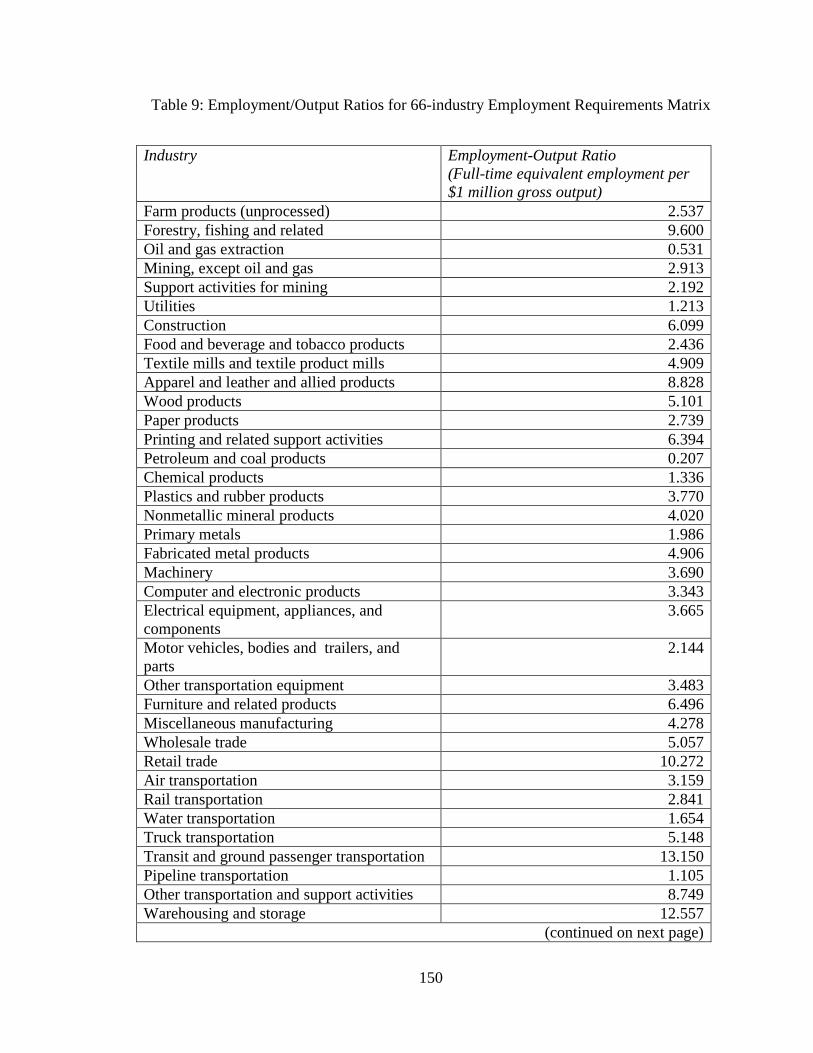
150
Table 9: Employment/Output Ratios for 66-industry Employment Requirements Matrix
Industry Employment-Output Ratio (Full-time equivalent employment per $1 million gross output)
Farm products (unprocessed) 2.537 Forestry, fishing and related 9.600 Oil and gas extraction 0.531 Mining, except oil and gas 2.913 Support activities for mining 2.192 Utilities 1.213 Construction 6.099 Food and beverage and tobacco products 2.436 Textile mills and textile product mills 4.909 Apparel and leather and allied products 8.828 Wood products 5.101 Paper products 2.739 Printing and related support activities 6.394 Petroleum and coal products 0.207 Chemical products 1.336 Plastics and rubber products 3.770 Nonmetallic mineral products 4.020 Primary metals 1.986 Fabricated metal products 4.906 Machinery 3.690 Computer and electronic products 3.343 Electrical equipment, appliances, and components
3.665
Motor vehicles, bodies and trailers, and parts
2.144
Other transportation equipment 3.483 Furniture and related products 6.496 Miscellaneous manufacturing 4.278 Wholesale trade 5.057 Retail trade 10.272 Air transportation 3.159 Rail transportation 2.841 Water transportation 1.654 Truck transportation 5.148 Transit and ground passenger transportation 13.150 Pipeline transportation 1.105 Other transportation and support activities 8.749 Warehousing and storage 12.557
(continued on next page)

151
(continued from previous page) Publishing industries (includes software) 3.090 Motion picture and sound recording industries
3.350
Broadcasting and telecommunications 1.724 Information and data processing services 2.478 Federal Reserve banks, credit intermediation, and related activities
3.799
Securities, commodity contracts, and investments
1.890
Insurance carriers and related activities 3.598 Funds, trusts, and other financial vehicles 0.890 Real estate 0.667 Rental and leasing services and lessors of intangible assets
2.266
Legal services 4.774 Miscellaneous professional, scientific and technical services
4.769
Computer systems design and related services
6.199
Management of companies and enterprises 4.378 Administrative and support services 12.903 Waste management and remediation services 4.625 Educational services 13.006 Ambulatory health care services 7.205 Hospitals and nursing and residential care facilities
10.440
Social assistance 17.996 Performing arts, spectator sports, museums, and related activities
4.705
Amusements, gambling, and recreation industries
11.818
Accommodation 9.056 Food services and drinking places 15.343 Other services, except government 10.291 Federal government enterprises 7.519 Federal general government 4.092 State and local government enterprises 4.693 State and local general government 9.293 Renewable Energy and Energy Efficiency 5.177

152
Table 10: Employment/Output Ratios from REEE Survey Data
Survey Industry Employment/Output Ratio (FTE Jobs per $1 million sales)
RE Production and Sales 3.16 Energy Services 5.54 Green Building 5.92 REEE(single industry) 5.18

153
Table 11: Employment Multipliers in Original and Expanded I-O Tables
Employment Multipliers (FTE Employment per $1 million demand)
Original 65x65 Table Expanded 66x66 Table Direct Indirect Total Direct Indirect Total Farms 3.03 4.45 7.48 2.94 3.57 6.51 Forestry, fishing, and related activities
13.98 2.25 16.23 13.66 2.13 15.79
Oil and gas extraction 0.64 1.62 2.26 0.64 1.54 2.18 Mining, except oil and gas 3.24 2.35 5.59 3.23 2.26 5.50 Support activities for mining 2.20 3.53 5.73 2.20 3.29 5.49 Utilities 1.22 1.68 2.90 1.22 1.57 2.79 Construction 6.13 4.56 10.69 6.13 4.46 10.58 Food and beverage and tobacco products
2.89 5.72 8.60 2.86 5.29 8.16
Textile mills and textile product mills
6.01 4.47 10.48 6.06 4.56 10.62
Apparel and leather and allied products
9.62 4.26 13.88 9.63 4.29 13.93
Wood products 6.55 6.50 13.06 6.49 6.37 12.85 Paper products 3.41 4.62 8.04 3.48 4.95 8.43 Printing and related support activities
6.63 4.09 10.72 6.63 4.12 10.75
Petroleum and coal products 0.23 2.82 3.06 0.23 2.75 2.99 Chemical products 1.80 3.65 5.44 1.79 3.55 5.34 Plastics and rubber products 4.07 4.54 8.61 4.06 4.47 8.53 Nonmetallic mineral products 4.50 3.68 8.18 4.45 3.65 8.11 Primary metals 2.80 3.70 6.50 2.91 4.17 7.08 Fabricated metal products 5.53 3.72 9.25 5.48 3.66 9.14 Machinery 4.03 4.57 8.61 3.99 4.38 8.36 Computer and electronic products 4.10 4.17 8.27 4.13 4.23 8.35 Electrical equipment, appliances, and components
3.90 3.69 7.59 3.86 3.55 7.41
Motor vehicles, bodies and trailers, and parts
3.04 5.91 8.95 3.05 5.95 9.00
Other transportation equipment 3.91 4.08 7.99 3.90 3.87 7.77 Furniture and related products 6.62 5.20 11.83 6.62 5.21 11.83 Miscellaneous manufacturing 4.54 4.17 8.71 4.51 3.98 8.48 Wholesale trade 5.26 2.26 7.53 5.26 2.17 7.43 Retail trade 10.33 2.53 12.87 10.33 2.42 12.75 Air transportation 3.17 4.22 7.39 3.17 4.60 7.77 Rail transportation 2.85 3.25 6.10 2.85 3.13 5.98 Water transportation 1.65 5.45 7.10 1.65 5.92 7.57
(continued on next page)

154
(continued from previous page) Truck transportation 5.92 3.62 9.54 5.90 3.51 9.41 Transit and ground passenger transportation
13.50 2.96 16.46 13.48 2.84 16.32
Pipeline transportation 1.13 3.74 4.87 1.13 3.57 4.70 Other transportation and support activities
9.12 1.58 10.70 9.11 1.51 10.62
Warehousing and storage 12.57 1.55 14.12 12.57 1.45 14.02 Publishing industries (includes software)
3.30 4.37 7.68 3.30 4.22 7.52
Motion picture and sound recording industries
4.41 3.13 7.54 4.40 3.03 7.44
Broadcasting and telecommunications
2.31 3.55 5.86 2.29 3.37 5.66
Information and data processing services
2.57 5.34 7.91 2.57 5.37 7.94
Federal Reserve banks, credit intermediation, and related activities
4.09 2.05 6.13 4.09 2.04 6.13
Securities, commodity contracts, and investments
2.35 2.64 4.99 2.33 2.50 4.83
Insurance carriers and related activities
5.70 1.37 7.07 5.60 1.27 6.88
Funds, trusts, and other financial vehicles
0.90 4.43 5.33 0.90 4.43 5.33
Real estate 0.71 2.29 3.00 0.70 2.16 2.86 Rental and leasing services and lessors of intangible assets
2.33 4.13 6.46 2.33 4.00 6.33
Legal services 4.97 2.16 7.13 4.96 2.01 6.96 Miscellaneous professional, scientific and technical services
5.38 3.21 8.60 5.27 2.87 8.14
Computer systems design and related services
6.24 2.67 8.91 6.24 2.47 8.70
Management of companies and enterprises
4.40 2.82 7.22 4.40 2.58 6.98
Administrative and support services
13.80 2.48 16.28 13.75 2.31 16.06
Waste management and remediation services
5.24 4.21 9.45 5.14 3.78 8.92
Educational services 13.10 2.84 15.94 13.09 2.50 15.59 Ambulatory health care services 7.32 2.60 9.91 7.31 2.41 9.72 Hospitals and nursing and residential care facilities
10.44 3.65 14.09 10.44 3.45 13.89
Social assistance 18.00 3.09 21.08 18.00 2.90 20.90 (continued on next page)

155
(continued from previous page) Performing arts, spectator sports, museums, and related activities
5.50 2.30 7.80 5.48 2.16 7.63
Amusements, gambling, and recreation industries
11.83 2.78 14.60 11.83 2.63 14.45
Accommodation 9.09 3.39 12.48 9.08 3.19 12.27 Food services and drinking places 15.53 3.78 19.31 15.52 3.56 19.08 Other services, except government 10.53 3.68 14.21 10.52 3.50 14.03 Federal government enterprises 7.54 2.27 9.81 7.52 3.07 10.59 Federal general government 4.09 3.64 7.73 4.10 2.55 6.65 State and local government enterprises
4.77 4.48 9.25 4.73 3.73 8.46
State and local general government
9.35 2.88 12.23 9.41 3.31 12.71
REEE n/a n/a n/a 5.24 2.06 7.29 Average Employment Multiplier 5.78 3.50 9.28 5.76 3.37 9.13 Average Manufacturing Multiplier 4.43 4.40 8.83 4.43 4.36 8.79 Average Non-Manufacturing Multiplier
6.34 3.13 9.47 6.32 2.98 9.30

156
Table 12: Total Employment Multipliers for Original, 65x65, and 68x68 I-O Tables
Total Employment Multipliers (FTE Employment per $1 million demand)
Original (65x65)
Single REEE Industry (66x66)
Three Distinct REEE Industries
(68x68) Farms 7.48 6.51 6.52 Forestry, fishing, and related activities 16.23 15.79 15.82 Oil and gas extraction 2.26 2.18 2.18 Mining, except oil and gas 5.59 5.50 5.51 Support activities for mining 5.73 5.49 5.50 Utilities 2.90 2.79 2.79 Construction 10.69 10.58 10.58 Food and beverage and tobacco products
8.60 8.16 8.16
Textile mills and textile product mills 10.48 10.62 10.62 Apparel and leather and allied products 13.88 13.93 13.92 Wood products 13.06 12.85 12.88 Paper products 8.04 8.43 8.43 Printing and related support activities 10.72 10.75 10.76 Petroleum and coal products 3.06 2.99 2.98 Chemical products 5.44 5.34 5.34 Plastics and rubber products 8.61 8.53 8.53 Nonmetallic mineral products 8.18 8.11 7.74 Primary metals 6.50 7.08 7.08 Fabricated metal products 9.25 9.14 9.14 Machinery 8.61 8.36 8.74 Computer and electronic products 8.27 8.35 8.35 Electrical equipment, appliances, and components
7.59 7.41 7.41
Motor vehicles, bodies and trailers, and parts
8.95 9.00 9.03
Other transportation equipment 7.99 7.77 7.77 Furniture and related products 11.83 11.83 11.83 Miscellaneous manufacturing 8.71 8.48 8.03 Wholesale trade 7.53 7.43 7.42 Retail trade 12.87 12.75 12.75 Air transportation 7.39 7.77 7.76 Rail transportation 6.10 5.98 5.99 Water transportation 7.10 7.57 7.57 Truck transportation 9.54 9.41 9.41 Transit and ground passenger transportation
16.46 16.32 16.32
(continued on next page)
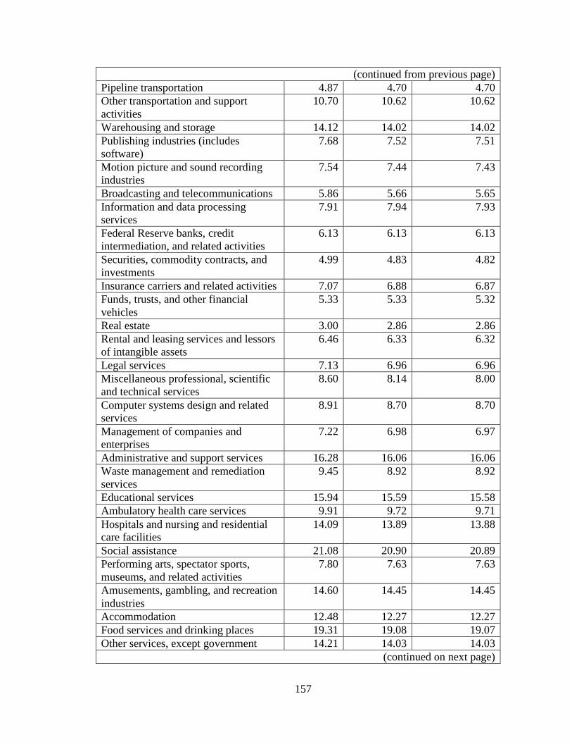
157
(continued from previous page) Pipeline transportation 4.87 4.70 4.70 Other transportation and support activities
10.70 10.62 10.62
Warehousing and storage 14.12 14.02 14.02 Publishing industries (includes software)
7.68 7.52 7.51
Motion picture and sound recording industries
7.54 7.44 7.43
Broadcasting and telecommunications 5.86 5.66 5.65 Information and data processing services
7.91 7.94 7.93
Federal Reserve banks, credit intermediation, and related activities
6.13 6.13 6.13
Securities, commodity contracts, and investments
4.99 4.83 4.82
Insurance carriers and related activities 7.07 6.88 6.87 Funds, trusts, and other financial vehicles
5.33 5.33 5.32
Real estate 3.00 2.86 2.86 Rental and leasing services and lessors of intangible assets
6.46 6.33 6.32
Legal services 7.13 6.96 6.96 Miscellaneous professional, scientific and technical services
8.60 8.14 8.00
Computer systems design and related services
8.91 8.70 8.70
Management of companies and enterprises
7.22 6.98 6.97
Administrative and support services 16.28 16.06 16.06 Waste management and remediation services
9.45 8.92 8.92
Educational services 15.94 15.59 15.58 Ambulatory health care services 9.91 9.72 9.71 Hospitals and nursing and residential care facilities
14.09 13.89 13.88
Social assistance 21.08 20.90 20.89 Performing arts, spectator sports, museums, and related activities
7.80 7.63 7.63
Amusements, gambling, and recreation industries
14.60 14.45 14.45
Accommodation 12.48 12.27 12.27 Food services and drinking places 19.31 19.08 19.07 Other services, except government 14.21 14.03 14.03
(continued on next page)
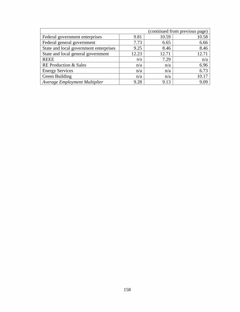
158
(continued from previous page) Federal government enterprises 9.81 10.59 10.58 Federal general government 7.73 6.65 6.66 State and local government enterprises 9.25 8.46 8.46 State and local general government 12.23 12.71 12.71 REEE n/a 7.29 n/a RE Production & Sales n/a n/a 6.96 Energy Services n/a n/a 6.73 Green Building n/a n/a 10.17 Average Employment Multiplier 9.28 9.13 9.09

159
Table 13: Composition of Synthetic REEE Industries
Synthetic Industry
Existing I-O Industry (65-industry level)
Weatherization Mass Transit
& Freight
Rail
Smart Grid
Wind Solar Biomass Green Program
Farm products (unprocessed)
0.0% 0.0% 0.0% 0.0% 0.0% 25.0% 2.50%
Forestry, fishing and related
0.0% 0.0% 0.0% 0.0% 0.0% 25.0% 2.50%
Construction 100.0% 45.0% 25.0% 26.0% 30.0% 25.0% 59.60% Chemical products
0.0% 0.0% 0.0% 0.0% 0.0% 12.5% 1.25%
Plastics and rubber products
0.0% 0.0% 0.0% 12.0% 0.0% 0.0% 1.20%
Fabricated metal products
0.0% 0.0% 0.0% 12.0% 17.5% 0.0% 2.95%
Machinery 0.0% 0.0% 25.0% 37.0% 0.0% 0.0% 6.20% Computer and electronic products
0.0% 0.0% 25.0% 3.0% 17.5% 0.0% 4.55%
Electrical equipment, appliances, and components
0.0% 0.0% 25.0% 3.0% 17.5% 0.0% 4.55%
Rail transportation
0.0% 10.0% 0.0% 0.0% 0.0% 0.0% 2.00%
Transit and ground passenger transportation
0.0% 45.0% 0.0% 0.0% 0.0% 0.0% 9.00%
Miscellaneous professional, scientific and technical services
0.0% 0.0% 0.0% 7.0% 17.5% 12.5% 3.70%
Note: The industries with zero values in all categories have been suppressed in this table.

160
Table 14: Employment Multipliers of Various REEE Industries Using Synthetic Approach
FTE Employment per $1 million demand Using original 65-industry I-O table
Direct Indirect Total Weatherization 6.13 4.56 10.69 Mass Transit & Freight Rail 9.12 3.71 12.83 Smart Grid 4.54 4.25 8.79 Wind 4.85 4.33 9.19 Solar 5.15 3.96 9.11 Biomass 6.68 3.67 10.36 “Green Program” 6.40 4.19 10.59

161
Table 15: Composition of Industries Using Hybrid Approach
Renewable Energy
Energy Services
Green Building
REEE
Forestry, fishing and related
0.05% 0.00% 1.12% 0.18%
Construction 16.00% 0.08% 28.53% 7.17% Food and beverage and tobacco products
0.23% 0.00% 0.00% 0.04%
Textile mills and textile product mills
0.01% 0.00% 0.00% 0.00%
Wood products 0.03% 0.54% 0.74% 0.48% Chemical products 1.44% 0.02% 0.19% 0.30% Plastics and rubber products
0.08% 0.09% 0.20% 0.10%
Nonmetallic mineral products
5.75% 0.00% 43.93% 7.63%
Fabricated metal products 8.80% 0.00% 0.24% 1.59% Machinery 3.12% 0.00% 0.00% 0.55% Computer and electronic products
0.79% 0.00% 0.00% 0.14%
Electrical equipment, appliances, and components
9.57% 0.00% 0.00% 1.69%
Miscellaneous manufacturing
43.05% 1.85% 1.39% 9.05%
Air transportation 0.06% 0.00% 0.00% 0.01% Truck transportation 0.01% 0.00% 0.52% 0.08% Transit and ground passenger transportation
0.02% 0.00% 0.00% 0.00%
Other transportation and support activities
0.07% 0.00% 0.00% 0.01%
Publishing industries (includes software)
0.02% 0.14% 0.00% 0.10%
Information and data processing services
0.00% 0.01% 0.00% 0.00%
Funds, trusts, and other financial vehicles
0.04% 0.00% 0.00% 0.01%
Miscellaneous professional, scientific and technical services
1.19% 30.09% 22.91% 23.91%
Waste management and remediation services
0.00% 53.16% 0.00% 35.78%
Educational services 0.01% 13.77% 0.25% 9.31% (continued on next page)

162
(continued from previous page) Amusements, gambling, and recreation industries
0.06% 0.00% 0.00% 0.01%
Accommodation 0.00% 0.02% 0.00% 0.01% Federal general government
9.46% 0.11% 0.00% 1.74%
State and local general government
0.13% 0.14% 0.00% 0.11%

163
Table 16: Employment Multipliers Using Hybrid Approach – Survey Responses as Demand Stimulus
Direct Indirect Total RE Production & Sales 4.74 4.06 8.81 Energy Services 6.36 3.73 10.09 Green Building 5.31 3.84 9.15 REEE 5.92 3.80 9.72

164
Table 17: Specification Tests for the Green Program
Green Program Specification
Share of Manufacturing Industries
Share of non-Manufacturing Industries
Total Employment Multiplier
Percentage Point Change in Share of Manufacturing versus Non-Manufacturing
Percentage Change in Total Employment Multiplier
Original 20.7% 79.3% 10.59 -- Alt 1 30.7% 69.3% 10.29 10 (more mfg) -2.83% Alt 2 10.7% 89.3% 10.89 10 (less mfg) 2.83% Alt 3 40.7% 59.3% 9.99 20 (more mfg) -5.66% Alt 4 0.7% 99.3% 11.19 20 (less mfg) 5.66% Alt 5 50.7% 49.3% 9.69 30 (more mfg) -8.49%

165
Table 18: Specification Tests for the REEE Industry
REEE Industry Specification
Share of Manufacturing Industries
Share of non-Manufacturing Industries
Total Employment Multiplier
Percentage Point Change in Share of Manufacturing versus Non-Manufacturing
Percentage Change in Total Employment Multiplier
Original 21.6% 78.4% 9.72 -- Alt 1 31.6% 68.4% 9.57 10 (more mfg) -1.57% Alt 2 11.6% 88.4% 9.88 10 (less mfg) 1.57% Alt 3 41.6% 58.4% 9.42 20 (more mfg) -3.15% Alt 4 1.6% 98.4% 10.03 20 (less mfg) 3.15% Alt 5 51.6% 48.4% 9.26 30 (more mfg) -4.72%
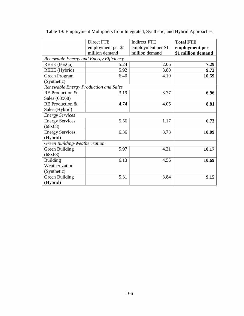
166
Table 19: Employment Multipliers from Integrated, Synthetic, and Hybrid Approaches
Direct FTE employment per $1 million demand
Indirect FTE employment per $1 million demand
Total FTE employment per $1 million demand
Renewable Energy and Energy Efficiency REEE (66x66) 5.24 2.06 7.29 REEE (Hybrid) 5.92 3.80 9.72 Green Program (Synthetic)
6.40 4.19 10.59
Renewable Energy Production and Sales RE Production & Sales (68x68)
3.19 3.77 6.96
RE Production & Sales (Hybrid)
4.74 4.06 8.81
Energy Services Energy Services (68x68)
5.56 1.17 6.73
Energy Services (Hybrid)
6.36 3.73 10.09
Green Building/Weatherization Green Building (68x68)
5.97 4.21 10.17
Building Weatherization (Synthetic)
6.13 4.56 10.69
Green Building (Hybrid)
5.31 3.84 9.15

167
Table 20: Comparison with REEE multipliers from previous studies
Study Industry or Industry Group
Employment Multiplier
Direct Employment Only Singh and Fehrs (2001)
Wind, solar pv, coal 5.70 jobs/$1M (wind); 5.65 jobs/$1M (solar); 3.96 jobs/$1M (coal)
Direct only
Sterzinger (2006) Wind, solar, geothermal, biomass
5.30 jobs/$1 million Direct only
Direct plus Indirect Employment EWEA (2004) Wind (Europe) 11.21 jobs/€1
million44 Direct + indirect
Pollin, Heintz, Garrett-Peltier (2009)
Green Program (various efficiency and renewables)
11.93 jobs/$1 million
Direct+ indirect
Bezdek (2009) Various REEE 8.61 jobs/$1 million Direct + indirect Laitner et al (2007) Efficiency only 13.50 jobs/$1 million Direct + indirect “Green Program” (synthetic)
Efficiency, wind, solar, biomass
10.59 jobs/$1 million Direct + indirect
REEE (hybrid) Various renewables and efficiency
9.72 jobs/$1 million Direct + indirect
REEE (integrated) Various renewables and efficiency
7.29 jobs/$1 million Direct + indirect
Direct, Indirect, and Induced Employment Pollin, Heintz, Garrett-Peltier (2009)
Green Program (various efficiency and renewables)
16.70 jobs/$1 million (as reported)
Direct, indirect, induced
Roland-Holst (2008) Efficiency only 26.81 jobs/$1 million Direct, indirect, induced
44 Over the course of 2002, which the EWEA used as a base year for this multiplier, the Euro and the U.S. dollar exchanged for nearly 1 to 1, therefore we can compare this estimate to a jobs-per-dollar estimate.
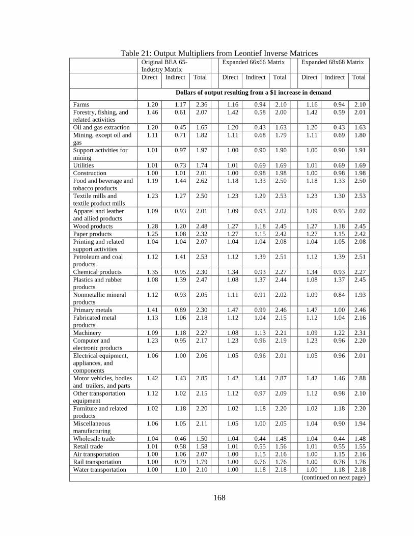
168
Table 21: Output Multipliers from Leontief Inverse Matrices Original BEA 65-
Industry Matrix Expanded 66x66 Matrix Expanded 68x68 Matrix
Direct Indirect Total Direct Indirect Total Direct Indirect Total
Dollars of output resulting from a $1 increase in demand
Farms 1.20 1.17 2.36 1.16 0.94 2.10 1.16 0.94 2.10 Forestry, fishing, and related activities
1.46 0.61 2.07 1.42 0.58 2.00 1.42 0.59 2.01
Oil and gas extraction 1.20 0.45 1.65 1.20 0.43 1.63 1.20 0.43 1.63 Mining, except oil and gas
1.11 0.71 1.82 1.11 0.68 1.79 1.11 0.69 1.80
Support activities for mining
1.01 0.97 1.97 1.00 0.90 1.90 1.00 0.90 1.91
Utilities 1.01 0.73 1.74 1.01 0.69 1.69 1.01 0.69 1.69 Construction 1.00 1.01 2.01 1.00 0.98 1.98 1.00 0.98 1.98 Food and beverage and tobacco products
1.19 1.44 2.62 1.18 1.33 2.50 1.18 1.33 2.50
Textile mills and textile product mills
1.23 1.27 2.50 1.23 1.29 2.53 1.23 1.30 2.53
Apparel and leather and allied products
1.09 0.93 2.01 1.09 0.93 2.02 1.09 0.93 2.02
Wood products 1.28 1.20 2.48 1.27 1.18 2.45 1.27 1.18 2.45 Paper products 1.25 1.08 2.32 1.27 1.15 2.42 1.27 1.15 2.42 Printing and related support activities
1.04 1.04 2.07 1.04 1.04 2.08 1.04 1.05 2.08
Petroleum and coal products
1.12 1.41 2.53 1.12 1.39 2.51 1.12 1.39 2.51
Chemical products 1.35 0.95 2.30 1.34 0.93 2.27 1.34 0.93 2.27 Plastics and rubber products
1.08 1.39 2.47 1.08 1.37 2.44 1.08 1.37 2.45
Nonmetallic mineral products
1.12 0.93 2.05 1.11 0.91 2.02 1.09 0.84 1.93
Primary metals 1.41 0.89 2.30 1.47 0.99 2.46 1.47 1.00 2.46 Fabricated metal products
1.13 1.06 2.18 1.12 1.04 2.15 1.12 1.04 2.16
Machinery 1.09 1.18 2.27 1.08 1.13 2.21 1.09 1.22 2.31 Computer and electronic products
1.23 0.95 2.17 1.23 0.96 2.19 1.23 0.96 2.20
Electrical equipment, appliances, and components
1.06 1.00 2.06 1.05 0.96 2.01 1.05 0.96 2.01
Motor vehicles, bodies and trailers, and parts
1.42 1.43 2.85 1.42 1.44 2.87 1.42 1.46 2.88
Other transportation equipment
1.12 1.02 2.15 1.12 0.97 2.09 1.12 0.98 2.10
Furniture and related products
1.02 1.18 2.20 1.02 1.18 2.20 1.02 1.18 2.20
Miscellaneous manufacturing
1.06 1.05 2.11 1.05 1.00 2.05 1.04 0.90 1.94
Wholesale trade 1.04 0.46 1.50 1.04 0.44 1.48 1.04 0.44 1.48 Retail trade 1.01 0.58 1.58 1.01 0.55 1.56 1.01 0.55 1.55 Air transportation 1.00 1.06 2.07 1.00 1.15 2.16 1.00 1.15 2.16 Rail transportation 1.00 0.79 1.79 1.00 0.76 1.76 1.00 0.76 1.76 Water transportation 1.00 1.10 2.10 1.00 1.18 2.18 1.00 1.18 2.18
(continued on next page)

169
(continued from previous page) Truck transportation 1.15 0.93 2.08 1.15 0.90 2.05 1.15 0.90 2.05 Transit and ground passenger transportation
1.03 0.80 1.82 1.03 0.76 1.78 1.03 0.76 1.78
Pipeline transportation 1.02 1.17 2.19 1.02 1.14 2.16 1.02 1.14 2.16 Other transportation and support activities
1.04 0.43 1.47 1.04 0.41 1.45 1.04 0.41 1.45
Warehousing and storage
1.00 0.41 1.41 1.00 0.38 1.38 1.00 0.38 1.38
Publishing industries (includes software)
1.07 0.91 1.98 1.07 0.88 1.95 1.07 0.88 1.95
Motion picture and sound recording industries
1.32 0.71 2.03 1.31 0.69 2.01 1.31 0.69 2.01
Broadcasting and telecommunications
1.34 0.77 2.11 1.33 0.73 2.06 1.33 0.73 2.06
Information and data processing services
1.04 1.07 2.11 1.04 1.08 2.12 1.04 1.08 2.12
Federal Reserve banks, credit intermediation, and related activities
1.08 0.45 1.53 1.08 0.46 1.53 1.08 0.45 1.53
Securities, commodity contracts, and investments
1.24 0.59 1.84 1.23 0.56 1.80 1.23 0.56 1.80
Insurance carriers and related activities
1.58 0.38 1.97 1.56 0.36 1.92 1.56 0.36 1.92
Funds, trusts, and other financial vehicles
1.01 1.44 2.44 1.01 1.45 2.46 1.01 1.45 2.46
Real estate 1.06 0.44 1.49 1.05 0.41 1.46 1.05 0.41 1.46 Rental and leasing services and lessors of intangible assets
1.03 0.81 1.84 1.03 0.78 1.81 1.03 0.78 1.81
Legal services 1.04 0.46 1.50 1.04 0.43 1.47 1.04 0.43 1.46 Miscellaneous professional, scientific and technical services
1.13 0.64 1.77 1.10 0.57 1.68 1.10 0.55 1.65
Computer systems design and related services
1.01 0.48 1.48 1.01 0.44 1.45 1.01 0.44 1.45
Management of companies and enterprises
1.01 0.70 1.70 1.01 0.64 1.64 1.01 0.64 1.64
Administrative and support services
1.07 0.62 1.69 1.07 0.58 1.65 1.07 0.58 1.65
Waste management and remediation services
1.13 1.04 2.17 1.11 0.95 2.06 1.11 0.95 2.06
Educational services 1.01 0.68 1.68 1.01 0.60 1.61 1.01 0.60 1.61 Ambulatory health care services
1.02 0.57 1.58 1.01 0.53 1.54 1.01 0.53 1.54
Hospitals and nursing and residential care facilities
1.00 0.84 1.84 1.00 0.80 1.80 1.00 0.79 1.79
Social assistance 1.00 0.73 1.73 1.00 0.69 1.69 1.00 0.69 1.69 (continued on next page)

170
(continued from previous page) Performing arts, spectator sports, museums, and related activities
1.17 0.48 1.65 1.16 0.45 1.61 1.16 0.45 1.61
Amusements, gambling, and recreation industries
1.00 0.64 1.64 1.00 0.60 1.60 1.00 0.60 1.60
Accommodation 1.00 0.72 1.72 1.00 0.67 1.67 1.00 0.67 1.67 Food services and drinking places
1.01 1.03 2.04 1.01 0.97 1.98 1.01 0.97 1.98
Other services, except government
1.02 0.91 1.93 1.02 0.86 1.89 1.02 0.87 1.89
Federal government enterprises
1.00 0.56 1.57 1.00 0.67 1.68 1.00 0.67 1.67
Federal general government
1.00 0.79 1.79 1.00 0.63 1.63 1.00 0.63 1.64
State and local government enterprises
1.02 1.18 2.19 1.01 0.88 1.89 1.01 0.88 1.89
State and local general government
1.01 0.69 1.70 1.01 0.88 1.89 1.01 0.88 1.89
REEE n/a n/a n/a 1.01 0.46 1.47 n/a n/a n/a RE Production & Sales n/a n/a n/a n/a n/a n/a 1.01 0.93 1.94 Energy Services n/a n/a n/a n/a n/a n/a 1.00 0.25 1.25 Green Building n/a n/a n/a n/a n/a n/a 1.01 0.91 1.92 Average for all Industries
1.11 0.86 1.97 1.10 0.83 1.93 1.10 0.83 1.93
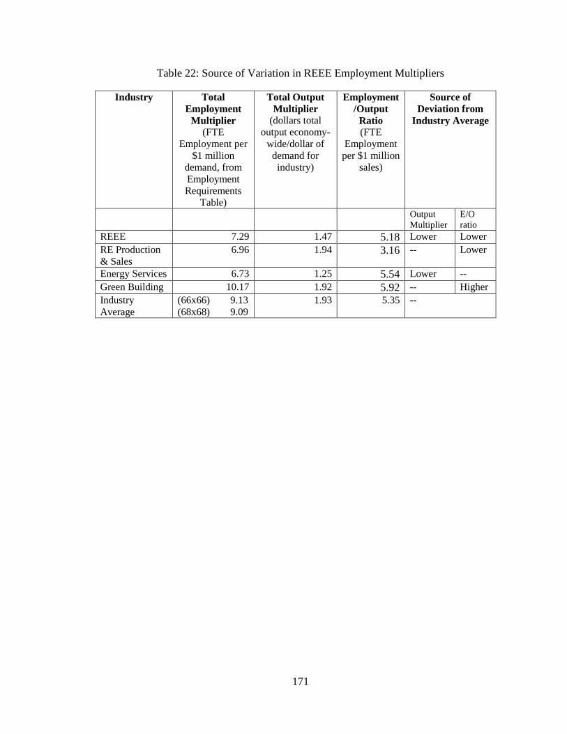
171
Table 22: Source of Variation in REEE Employment Multipliers
Industry Total Employment Multiplier
(FTE Employment per
$1 million demand, from Employment Requirements
Table)
Total Output Multiplier
(dollars total output economy-
wide/dollar of demand for industry)
Employment/Output Ratio (FTE
Employment per $1 million
sales)
Source of Deviation from
Industry Average
Output Multiplier
E/O ratio
REEE 7.29 1.47 5.18 Lower Lower RE Production & Sales
6.96 1.94 3.16 -- Lower
Energy Services 6.73 1.25 5.54 Lower -- Green Building 10.17 1.92 5.92 -- Higher Industry Average
(66x66) 9.13 (68x68) 9.09
1.93 5.35 --

172
Table 23: REEE Employment Multipliers Using Industry Average E/O Ratio
Industry Total Employment Multiplier (original)
Employment/Output Ratio (original)
Total Employment Multiplier
(using average E/O)
REEE 7.29 5.18 7.49 RE Production & Sales
6.96 3.16 9.16
Energy Services
6.73 5.54 6.54
Green Building 10.17 5.92 9.61 Industry Average
(66x66) 9.13 (68x68) 9.09
5.37 (66x66) 9.13 (68x68) 9.12
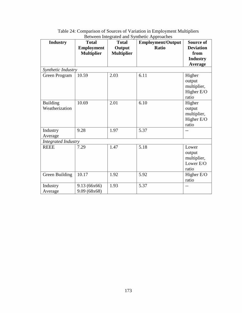
173
Table 24: Comparison of Sources of Variation in Employment Multipliers Between Integrated and Synthetic Approaches
Industry Total Employment Multiplier
Total Output
Multiplier
Employment/Output Ratio
Source of Deviation
from Industry Average
Synthetic Industry Green Program
10.59 2.03 6.11 Higher output multiplier, Higher E/O ratio
Building Weatherization
10.69 2.01 6.10 Higher output multiplier, Higher E/O ratio
Industry Average
9.28 1.97 5.37 --
Integrated Industry REEE 7.29 1.47 5.18 Lower
output multiplier, Lower E/O ratio
Green Building 10.17 1.92 5.92 Higher E/O ratio
Industry Average
9.13 (66x66) 9.09 (68x68)
1.93 5.37 --
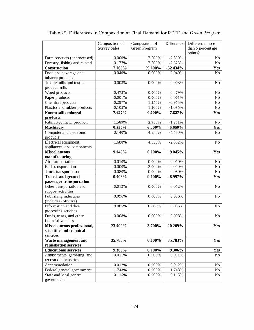
174
Table 25: Differences in Composition of Final Demand for REEE and Green Program
Composition of Survey Sales
Composition of Green Program
Difference Difference more than 5 percentage points?
Farm products (unprocessed) 0.000% 2.500% -2.500% No Forestry, fishing and related 0.177% 2.500% -2.323% No Construction 7.166% 59.600% -52.434% Yes Food and beverage and tobacco products
0.040% 0.000% 0.040% No
Textile mills and textile product mills
0.003% 0.000% 0.003% No
Wood products 0.479% 0.000% 0.479% No Paper products 0.001% 0.000% 0.001% No Chemical products 0.297% 1.250% -0.953% No Plastics and rubber products 0.105% 1.200% -1.095% No Nonmetallic mineral products
7.627% 0.000% 7.627% Yes
Fabricated metal products 1.589% 2.950% -1.361% No Machinery 0.550% 6.200% -5.650% Yes Computer and electronic products
0.140% 4.550% -4.410% No
Electrical equipment, appliances, and components
1.688% 4.550% -2.862% No
Miscellaneous manufacturing
9.045% 0.000% 9.045% Yes
Air transportation 0.010% 0.000% 0.010% No Rail transportation 0.000% 2.000% -2.000% No Truck transportation 0.080% 0.000% 0.080% No Transit and ground passenger transportation
0.003% 9.000% -8.997% Yes
Other transportation and support activities
0.012% 0.000% 0.012% No
Publishing industries (includes software)
0.096% 0.000% 0.096% No
Information and data processing services
0.005% 0.000% 0.005% No
Funds, trusts, and other financial vehicles
0.008% 0.000% 0.008% No
Miscellaneous professional, scientific and technical services
23.909% 3.700% 20.209% Yes
Waste management and remediation services
35.783% 0.000% 35.783% Yes
Educational services 9.306% 0.000% 9.306% Yes Amusements, gambling, and recreation industries
0.011% 0.000% 0.011% No
Accommodation 0.012% 0.000% 0.012% No Federal general government 1.743% 0.000% 1.743% No State and local general government
0.115% 0.000% 0.115% No
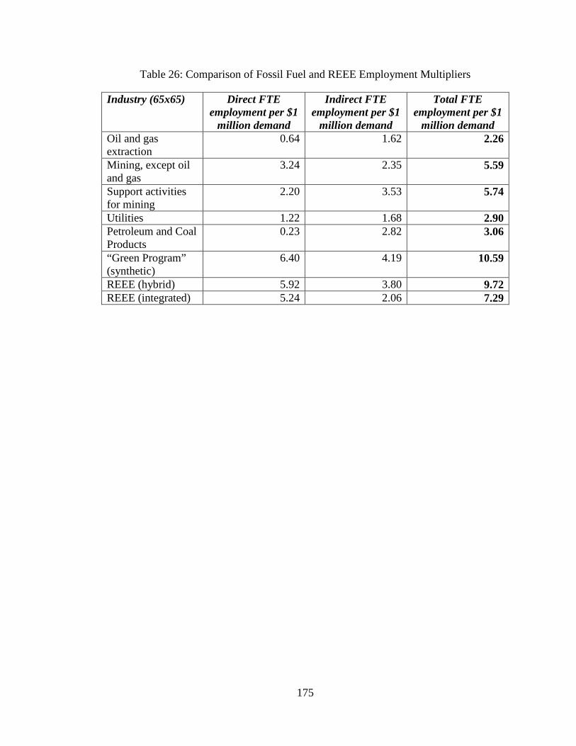
175
Table 26: Comparison of Fossil Fuel and REEE Employment Multipliers
Industry (65x65) Direct FTE employment per $1
million demand
Indirect FTE employment per $1
million demand
Total FTE employment per $1
million demand Oil and gas extraction
0.64 1.62 2.26
Mining, except oil and gas
3.24 2.35 5.59
Support activities for mining
2.20 3.53 5.74
Utilities 1.22 1.68 2.90 Petroleum and Coal Products
0.23 2.82 3.06
“Green Program” (synthetic)
6.40 4.19 10.59
REEE (hybrid) 5.92 3.80 9.72 REEE (integrated) 5.24 2.06 7.29

176
Figure 1: Employment impacts of alternative energy sources, Table 4 from (Pollin, Heintz, & Garrett-Peltier, 2009)

177
Figure 2: Energy Industries and Weights, from (Pollin, Heintz, & Garrett-Peltier, 2009)

178
APPENDIX
SURVEY QUESTIONNAIRE
ID
PLEASE RETURN BY May 16, 2008
Any questions, please call (413) 577-0818 or email [email protected]
Year of Reporting Information from calendar year
ending… Or, information from fiscal year ending…
Item 1: Business Type
1a. What is the primary purpose of your business? What do you produce or what type of service do you offer?
1b. Please mark an "X" next to the ownership structure that best corresponds to your business: Private – Corporate Private – Partnership/Proprietorship Private - Cooperative Publicly traded Non-Profit - Cooperative Non-profit
Renewable Energy and Energy Efficiency Survey of Employment, Sales and Costs
The information provided in this questionnaire is completely confidential. The data will be aggregated with data of other similar businesses, so that any publicly released data will not be traceable to the individual businesses who respond to this survey.
Reporting Instructions: This questionnaire is designed to assess the purchases and sales made by businesses in the renewable energy and energy efficiency sector. Please read the instructions in each section carefully. Provide exact figures when possible and reasonable estimates in other cases. PLEASE RESPOND TO ALL QUESTIONS. Please provide information for the year 2005 if possible. If not possible, please provide information for 2006 or 2007 (or a recent fiscal year which does not correspond to a calendar year), and please note the year for which the information is provided.

179
Government
Other (please describe)
Item 2: Employment
Enter amount
here 2a. Number of Employees at the end of 2005 (or end of fiscal year for which you are reporting)
2b. Total compensation for employees in 2005
Total Wages $ Total Benefits $
2c. Employment by occupation. Next to each occupational category below, please list the number of persons employed in each occupation. Please separate full-time and part-time, and list how many hours (on average) a part-time employee works.
Occupational Category
# of Full-time employees in this
position
# of Part-time employees in this
position
Average # of weekly hours worked by a P/T employee (per
occupation) Management Business and Financial Operations Computer and Math Occupations Architecture & Engineering Life, Physical and Social Science Community and Social Service Legal Education and Training Arts, Design, Entertainment, Sports Healthcare Healthcare Support Protective Service Food Prep and Related Cleaning and Maintenance Personal Care Sales and Related Office and Administrative Support Farming, Fishing, Forestry Construction/Extraction Installation, Maintenance, Repair Production Transportation and Moving Military-specific occupations Other (please list occupational titles)
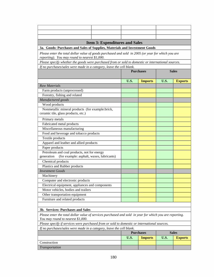
180
Item 3: Expenditures and Sales 3a. Goods: Purchases and Sales of Supplies, Materials and Investment Goods
Please enter the total dollar value of goods purchased and sold in 2005 (or year for which you are reporting). You may round to nearest $1,000. Please specify whether the goods were purchased from or sold to domestic or international sources. If no purchases/sales were made in a category, leave the cell blank.
Purchases Sales
U.S. Imports U.S. Exports Raw Materials Farm products (unprocessed) Forestry, fishing and related Manufactured goods Wood products Nonmetallic mineral products (for example:brick, ceramic tile, glass products, etc.) Primary metals Fabricated metal products Miscellaneous manufacturing Food and beverage and tobacco products Textile products Apparel and leather and allied products Paper products Petroleum and coal products, not for energy generation (for example: asphalt, waxes, lubricants) Chemical products Plastics and Rubber products Investment Goods Machinery Computer and electronic products Electrical equipment, appliances and components Motor vehicles, bodies and trailers Other transportation equipment Furniture and related products
3b. Services: Purchases and Sales
Please enter the total dollar value of services purchased and sold in year for which you are reporting. You may round to nearest $1,000. Please specify if services were purchased from or sold to domestic or international sources. If no purchases/sales were made in a category, leave the cell blank.
Purchases Sales
U.S. Imports U.S. Exports Construction Transportation
181
Air Transportation Rail Transportation Water Transportation Truck Transportation Transit and Ground Passenger Transportation Pipeline Transportation Other transportation Warehousing and Storage Information U.S. (P) Imports U.S. (S) Exports Publishing Industries (incl. software) Motion picture and sound recording Broadcasting and telecommunications Information and data processing services Finance and Insurance Insurance (DO NOT include here health insurance costs already listed above) Financing and banking Real Estate Professional and Business Services Legal Services Accounting and Bookkeeping Advertising/Marketing and related Computer Systems design and related Architecture/Engineering Scientific R & D Misc. Scientific, Professional and Technical Services Management of companies Administrative and Support Services Waste Management Educational Services Health Care Services Arts, Entertainment and Recreation Accommodation Food Services Federal Government services State/local government services 3c. Annual Revenues and Expenses Please enter the total amount of revenues and expenses in year for which you are reporting. You may round to nearest $1,000. Please include totals from ALL PARTS of this questionnaire (including 4 and 5).
Total Gross Revenue from all sources $ Total Expenses $
Item 4: Energy purchases and production 4a. Purchased Energy
Please enter the total dollar value of energy purchased in year for which you are reporting. You may round to nearest $1,000. If no purchases were made in a category, leave the category blank.

182
If you did not purchase energy goods directly, but purchased electricity and heat, please list these purchases and identify the main source of energy if you know it. Oil $ Natural Gas $ Coal $ Hydroelectric $ Nuclear $ Solar PV $ Solar thermal $ Wind $ Geothermal $ Biomass Solid Biomass fuels (e.g. sawdust, crop wastes) $ Liquid Biomass fuels (e.g. biodiesel, ethanol) $ Gaseous biomass fuels (e.g. biogas, methane) $ Electricity (please identify major source if
known) Source:
$ Heat (please identify major source if
known) Source:
$ Renewable Energy Certificates/offsets (please identify type of energy source if known) $ Other (please describe)
4b. Produced Energy
Please enter below the total amount of energy your business produced both for its own use and for sale in year for which you are reporting. When possible, please list both the quantity of energy produced and the dollar value of energy produced. Production
for sale (in $)
Production for sale (BTU or other physical units)
Production for own use (equivalent $ value)
Production for own use (BTU or other physical
units)
Oil Natural Gas Coal Hydroelectric
Nuclear Solar PV Solar thermal Wind Geothermal Biomass Solid biomass fuels

183
Liquid biomass fuels
Gaseous biomass fuels
Item 5: Other Income and Expenses 5a. Other income and public support. Please describe and list amounts and sources of any subsidies, tax credits, or other public support you received in year for which you are reporting.
Description of Subsidy/Tax Incentive
U.S. State/Local U.S. Federal Foreign
(1) $ $ $
(2) $ $ $
(3) $ $ $
(4) $ $ $
(5) $ $ $ 5b. Other expenses. Please enter the dollar value of other expenses incurred in year for which you are reporting.
Lease and Rental Payments $ Taxes and License Fees (except payroll taxes) $ Payroll Taxes $ Depreciation and Amortization Expenses $ Interest Expense $ Other (please describe)
Item 6: Other relevant information. Please use this space or attach a separate sheet for explanations of items on the questionnaire or to add any additional information that you think might be relevant.
Item 7: Contact Information. Please list the name and contact information for the person or persons who filled out this survey, along with contact information for other persons in the business who could answer questions regarding its content. (Note: this section is optional, but may be useful in clarifying answers to survey questions and for contacting the relevant persons once results are tallied.)
Name Phone Email
Thank you very much for your cooperation! Please return this form by email to: [email protected]
or by fax to: (413) 577-0261 or by mail to: Political Economy Research Institute
Green Jobs Survey Project 418 N. Pleasant Street
Amherst, MA 01002

184
BIBLIOGRAPHY
Ackerman, F., Stanton, E., DeCanio, S., Goodstein, E., Howarth, R., Norgaard, R., et al. (2008). The Economics of 350: The Benefits and Costs of Climate Stabilization. Portland, OR: Economics for Equity and Environment.
American Solar Energy Society and Management Information Services, Inc. . (2008). Defining, Estimating, and Forecasting the Renewable Energy Industries in the U.S. and Colorado. Boulder, CO: American Solar Energy Society.
Berck, P., & Hoffman, S. (2002). Assessing the Employment Impacts of Environmental and Natural Resource Policy. Environmental and Resource Economics , 22, 133-156.
Bezdek, R. H. (2009). Estimating the Jobs Impacts of Tackling Climate Change. Boulder, CO: Management Information Systems Inc., for the American Solar Energy Society.
Clarke, L., Edmonds, J., Jacoby, H., Pitcher, H., Reilly, J., & Richels, R. (2007). "Scenarios of Greenhouse Gas Emissions and Atmospheric Concentrations," Sub-Report 2.1A of Synthesis and Assessment Product 2.1 by the. Washington, D.C.: Dept of Energy, Office of Biological & Environmental Research.
Ehrhardt-Martinez, K., & Laitner, J. A. (2008). The Size of the U.S. Energy Efficiency Market: Generating a More Complete Picture. Washington, D.C.: American Council for an Energy-Efficient Economy.
European Wind Energy Association. (2004). Wind Energy - The Facts. Retrieved 2006, from www.ewea.org/fileadmin/ewea_documents/documents/publications/WETF/WETF.pdf
Fawcett, A. A., Calvin, K. V., de la Chesnaye, F., Reilly, J. M., & Weyant, J. P. (2009). Overview of EMF 22 U.S. transition scenarios. Energy Policy , 31, S198-S211.
Groves, R. (2006). Experiments in Producing Non-Response Bias. Public Opinion Quarterly , 70 (5), 720-735.
Hillebrand, B., Buttermann, H. G., Behringer, J. M., & Bleuel, M. (2006). The expansion of renewable energies and employment effects in Germany. Energy Policy , 34, 3484-3494.
Horowitz, K. J., & Planting, M. A. (2006). Concepts and Methods of the Input-Output Accounts. Washington, D.C.: Bureau of Economic Analysis, U.S. Dept. of Commerce.

185
Keeter, S., Kennedy, C., Dimock, M., Best, J., & Craighill, P. (2006). Gauging the Impact of Growing Non-Response on Estimates from a National RDD Telephone Survey. Public Opinion Quarterly , 70 (5), 739-779.
Kim, S. j., Davis, V. A., Jacobson, A. M., & Lyndaker, A. S. (2008). Annual Industry Accounts: Revised Statistics for 2005-2007. Washington, D.C.: Bureau of Economic Analysis.
Laitner, J. A. (2009). The Positive Economics of Climate Change Policies: What the Historical Evidence Can Tell Us. Washington, D.C.: American Council for an Energy-Efficient Economy, ACEEE Report No. E095.
Laitner, J. A., Eldridge, M., & Elliot, R. N. (2007). The Economic Benefits of an Energy Efficiency and Onsite Renewable Energy Strategy to Meet Growing Electricity Needs in Texas. Washington, D.C.: American Council for an Energy-Efficient Economy, ACEEE Report #E076.
Leontief, W. (1986). Input Output Economics, 2nd ed. New York: Oxford University Press.
McKinsey & Company and The Conference Board. (2007). Reducing U.S. Greenhouse Gas Emissions: How Much at What Cost? Syndney, Australia: McKinsey & Company.
McKinsey Global Institute. (2007). Curbing Global Energy Demand Growth: The Energy Productivity Opportunity. Syndney, Australia: McKinsey & Company.
McKinsey Global Institute. (2008). The carbon productivity challenge: Curbing climate change and sustaining economic growth. Sydney, Australia: McKinsey & Company.
Miller, R. E., & Blair, P. D. (1985). Input-Output Analysis: Foundations and Extensions. New Jersey: Prentice-Hall, Inc.
National Academy of Sciences. (2010 (pre-publication copy)). Real Prospects for Energy Efficiency in the United States. Washington, D.C.
Nordhaus, W. (2008). A Question of Balance. New Haven, CT: Yale University Press.
Paltsev, S., Reilly, J. M., Jacoby, H. D., & Morris, J. F. (2009). The cost of climate policy in the United States. Energy Policy , 31, S235-S243.
Parry, M., Canziani, O., Palutikof, J., van der Linden, P., Hanson, C., & Eds. (2007). IPCC, 2007: Climate Change 2007: Impacts, Adaptation and Vulnerability. Contribution of Working Group II to the Fourth Assessment. Cambridge, UK: Cambridge University Press.

186
Pollin, R., & Garrett-Peltier, H. (2009). The U.S. Employment Effects of Military and Domestic Spending Priorities: An Updated Analysis. Amherst, MA and Washington D.C.: Political Economy Research Institute and the Institute for Policy Studies.
Pollin, R., Heintz, J., & Garrett-Peltier, H. (2009). The Economic Benefits of Investing in Clean Energy: How the Economic Stimulus Program and New Legislation Can Boost U.S. Economic Growth and Employment. Amherst, MA and Washington D.C.: Political Economy Research Institute and Center for American Progress.
Richardson, H. W. (1972). Input-Output and Regional Economics. New York: John Wiley and Sons.
Ross, M. T., Fawcett, A. A., & Clapp, C. S. (2009). U.S. climate mitigation pathways post-2012: Transition scenarios in ADAGE. Energy Policy , 31, S212-S222.
Salant, P., & Dillman, D. A. (1994). How to Conduct Your Own Survey. New York: John Wiley & Sons.
Schneider, S., Semenov, S., Patwardhan, A., Burton, I., Magadza, C., Oppenheimer, M., et al. (2007). Assessing Key Vulnerabilities and the Risk From Climate Change. In M. Parry, O. Canziani, J. Palutikof, P. van der Linden, & C. Hanson (Eds.), Climate Change 2007: Impacts, Adaptation and Vulnerability. Contribution of Working Group II to the Fourth Assessment Report of the Intergovernmnetal Panel on Climate Change (pp. 779-810). Cambridge, UK: Cambridge University Press.
Scott, M. J., Roop, J. M., Schultz, R. W., Anderson, D. M., & Cort, K. A. (2008). The impact of DOE building technology energy efficiency programs on U.S. employment, income, and investment. Energy Economics , 30, 2283-2301.
Singh, V., & Fehrs, J. (2001). The Work That Goes Into Renewable Energy. Washington, D.C.: Renewable Energy Policy Project, REPP Report #13.
Stern, S. N. (2007). The Economics of Climate Change: The Stern Review. Cambridge, U.K.: Cambridge University Press.
Sterzinger, G. (2006). Jobs and Renewable Energy Project: Final Technical Report . Washington D.C.: Submitted to the U.S. Dept. of Energy by the Renewable Energy Policy Project.
Sterzinger, G., & Svrcek, M. (2005). Component Manufacturing: Ohio's Future in the Renewable Energy Industry. Washington, D.C.: Renewable Energy Policy Project.
Stone, R. (1961). Input-Output and National Accounts. Paris: Organisation for Economic Co-operation and Development.

187
Taylor, L. (. (1990). Socially Relevant Policy Analysis: Structuralist Computable General Equilibrium Models for the Developing World. Cambridge, MA: Massachusetts Institute of Technology.
The Perryman Group. (2003). Redefining the Prospects for Sustainable Prosperity, Employment Expansion, and Environmental Quality in the US: An Assessment of the Economic Impact of the Initiatives Comprising the Apollo Project. Waco, TX: Apollo Alliance.
U.S. Energy Information Administration. (2010). Annual Energy Outlook 2010 Early Release. Washington, D.C.
Wei, M., Patadia, S., & Kammen, D. (2010). Putting renewables and energy efficiency to work: How many jobs can the clean energy industry generate in the US? Energy Policy , 38, 919-931.