THE ELIMINATION OF THE INFINITE POLE IN THE POLE-DIPOLE ...

THE ELIMINATION OF THE INFINITE POLE IN THE POLE-DIPOLE

RESISTIVITY ARRAY

A Thesis submitted to The Graduate Studies and Research in partial fulfilment

of the requirements for a degree in Master of Science from the

Department of Geological Sciences,

University of Saskatchewan

Saskatoon, Saskatchewan

By

Xiao Xia Liang

c©Copyright Xiao Xia Liang, December 2015. All rights reserved.

Permission to Use

In submission of this thesis as a partial fulfilment for a postgraduate degree from the Uni-

versity of Saskatchewan, I agree for this University’s libraries to make copies of this thesis

for any academic related reviews or inspections. Due recognition is given to the University

of Saskatchewan and myself.

Any use in part or in full of this thesis for capital gain is not permitted without my written

permission. Academic or scholarly use of this thesis in part or in full will require permission

from the supervising professor, or from the University of Saskatchewan, Geological Sciences

department head.

Head of the Department of Geological Sciences

University of Saskatchewan

114 Science Place

Saskatoon, Saskatchewan

S7N 5E2

i

Abstract

The pole-dipole (PD) electrical resistivity array is used as part of a geophysical technique,

which can be used in exploration for mineral, geothermal and hydrological resources. Fur-

thermore, it can be used in archaeological investigations. The PD array is useful in obtaining

large depths of investigation, but the array requires one pole to be planted at a greater

distance from the other electrodes. Placing the infinite pole is time consuming and costly,

especially in rough terrains. It can also be a liability in populated areas. Previous data in-

version software assumes the infinite pole to be planted at infinity. Therefore, the field data

collected has to mimic the assumptions of the inversion software.

Some recent inversion programs use all 4-electrode positions for data inversion. In this case,

is a good approximation of infinity for the infinite pole still necessary? Is the depth of inves-

tigation still the same or relevant with a non-infinite, infinite pole? Is the resolution of the

cross-sections retained?

To answer the above questions a Generalized Electrode Array (GEA) 1 dimensional (1D)

inversion program is used. Different sets of field data were collected with non-infinite pole

(NIP) PD arrays; these arrays are set up as PD arrays with an infinite pole planted relatively

close to or on the survey lines itself. A COMSOL finite element model were modelled with

varying infinite pole distances to identify the distance required for the retention of the depth

ii

of investigation and resolution of the PD array.

Modelling from GEA shows the NIP distances do not affect the 1D inversion accuracy of

the resistivity nor the layer thickness. The field data indicates that it is necessary to have

an infinite pole, but the distance to the infinite pole can be substantially less than 10 times

the array length, which is the usual rule of thumb for infinite pole placement. With 3 dimen-

sional (3D) COMSOL modelling results, it indicates a minimum pole distance to be 2.5-array

length to retain the depth of investigation and precision of the inverted sections of the PD

array.

iii

Acknowledgements

I would like to thank Cameco for funding this thesis and Dr. Jim Merriam for the opportu-

nity to work with him as his student.

I also would like to thank the following people:

Dr. Sam Butler (University of Saskatchewan)

Jochen Kursawe (Oxford University)

Lloyd Litwin (University of Saskatchewan)

Susan Nehzati (University of Saskatchewan)

Robert Zschuppe

Michael Zhang (University of Saskatchewan)

Lastly, I would like to thank all of my family and friends for their love and support.

iv

Contents

Permission to Use i

Abstract ii

Acknowledgements iv

List of Figures vii

List of Tables xx

1 Introduction 1

1.1 Thesis and research objective . . . . . . . . . . . . . . . . . . . . . . . . . . 1

1.2 Electrical properties of materials . . . . . . . . . . . . . . . . . . . . . . . . . 3

1.3 Basics of Resistivity arrays . . . . . . . . . . . . . . . . . . . . . . . . . . . . 4

1.4 Depth of investigation and sensitivity using the Frechet derivative . . . . . . 13

1.5 Cross-correlation analytics . . . . . . . . . . . . . . . . . . . . . . . . . . . . 17

1.6 Uranium exploration using PD resistivity array . . . . . . . . . . . . . . . . 17

2 Methods 22

2.1 GEA 1D modelling . . . . . . . . . . . . . . . . . . . . . . . . . . . . . . . . 22

2.2 Field data . . . . . . . . . . . . . . . . . . . . . . . . . . . . . . . . . . . . . 25

2.3 Geoelectric COMSOL modelling . . . . . . . . . . . . . . . . . . . . . . . . . 26

v

3 Data Analysis and Results 30

3.1 GEA 1D inversions . . . . . . . . . . . . . . . . . . . . . . . . . . . . . . . . 30

3.2 Field data . . . . . . . . . . . . . . . . . . . . . . . . . . . . . . . . . . . . . 40

3.2.1 Field data inversions . . . . . . . . . . . . . . . . . . . . . . . . . . . 40

3.2.2 Field data sensitivity sections . . . . . . . . . . . . . . . . . . . . . . 41

3.2.3 Field data cross-correlation sections . . . . . . . . . . . . . . . . . . . 46

3.3 Geoeletric COMSOL modelling . . . . . . . . . . . . . . . . . . . . . . . . . 50

3.3.1 COMSOL model inversions . . . . . . . . . . . . . . . . . . . . . . . 50

3.3.2 COMSOL model sensitivity sections . . . . . . . . . . . . . . . . . . . 55

3.3.3 COMSOL model cross-correlation sections . . . . . . . . . . . . . . . 61

4 Conclusion and Discussions 71

4.1 GEA 1D data . . . . . . . . . . . . . . . . . . . . . . . . . . . . . . . . . . . 71

4.2 Field Data . . . . . . . . . . . . . . . . . . . . . . . . . . . . . . . . . . . . . 72

4.3 Geoelectric COMSOL modelling . . . . . . . . . . . . . . . . . . . . . . . . . 72

4.4 Discussions . . . . . . . . . . . . . . . . . . . . . . . . . . . . . . . . . . . . 73

References 74

Appendix A Electrode positioning for 1D GEA inversions 79

Appendix B Inverted sections from Field Data 84

Appendix C Sensitivity sections from Field Data 92

Appendix D Cross-correlation sections from Field Data 99

Appendix E Inverted sections from COMSOL modelling 107

Appendix F Sensitivity sections from COMSOL modelling 117

vi

Appendix G Cross-correlation sections from COMSOL modelling 126

vii

List of Figures

1.3.1 An illustration of a multi-node Wenner-α array system. C1 and C2 are in-

jection electrodes. P1 and P2 are potential electrodes. The red dot is where

the apparent resistivity measured is plotted using the pseudo-depth of unit

electrode spacing depth. The pseudodepth will be discussed in more details

in section 1.4. . . . . . . . . . . . . . . . . . . . . . . . . . . . . . . . . . . 5

1.3.2 An explanation of apparent resistivity. . . . . . . . . . . . . . . . . . . . . . 7

1.3.3 A comparison of a pseudosection and inverted section. . . . . . . . . . . . . 8

1.3.4 Diagram is showing a current flowing through an object with a cross sectional

area of A and length of l. . . . . . . . . . . . . . . . . . . . . . . . . . . . . 9

1.3.5 Diagram is showing a single injection point of current into a homogeneous

half space. The half circles are the equipotential surfaces and the current flow

intercepts the equipotential surfaces at 90 degrees. . . . . . . . . . . . . . . 10

1.3.6 Diagram containing four-electrode array with 2 potential electrodes P1 and

P2 and 2 injection electrodes C1 and C2. The potential measurement between

each injection electrodes and potential electrodes are seen as V1, V2, V3 and V4.

The corresponding distances between the potential and injection electrodes

are denoted by r1, r2, r3 and r4. . . . . . . . . . . . . . . . . . . . . . . . . 10

viii

1.3.7 Most commonly used arrays are outlined with its configuration. The arrays

include: Wenner-α, Wenner- β, pole-pole, pole-dipole, dipole-dipole equato-

rial, dipole-dipole axial. C1 and C2 are current injection electrodes. P1 and

P2 are potential electrodes. . . . . . . . . . . . . . . . . . . . . . . . . . . . 12

1.4.1 DOI values calculated using Butler’s (2015) Zmean equation. The array length

is normalized to 1. . . . . . . . . . . . . . . . . . . . . . . . . . . . . . . . 16

1.6.1 Map of the Athabasca Basin in northern Saskatchewan. Athabasca Basin is

outlined with the solid orange line. Seen here are some of the unconformity-

type uranium depositions. This map is taken from Overview of Cameco Ex-

ploration Athabasca Basin 2011, presentation by John Halaburda. . . . . . 18

1.6.2 A map of the Dawn Lake area in northern Saskatchewan. The PD electric

resistivity survey lines can be seen on the map. Each survey line is 1400

metres long. The electrode spacing is 25 metres. The data used to invert

Figure 1.6.3 is from line L15E seen in red. This map is modified from the

map provided by Cameco. . . . . . . . . . . . . . . . . . . . . . . . . . . . . 20

1.6.3 Inverted cross section of PD resistivity survey of uranium ore deposit in

northern Saskatchewan. Part of the ore deposit is seen at the bottom of the

section. A fault can be seen at the 1000 metres mark diagonally going down

to the 1300 metres mark. . . . . . . . . . . . . . . . . . . . . . . . . . . . . 21

2.1.1 Diagram of infinite one-dimensional GEA forward model. The model con-

tains two layers; the first layer is one meter and two meters thick with the

conductive models having 100Ωm in the top layer and the bottom contain-

ing infinite thickness with a 10Ωm resistivity. In reverse, the resistive models

have a 100Ωm top layer and a 10Ωm bottom layer. C1 and C2 are injection

electrodes. C2 is the infinite pole. P1 and P2 are potential electrodes. . . . . 23

ix

2.1.2 An example of a GEA inversion process. This is a conductive model with

one-meter upper layer thickness. The top layer is 10Ωm and the lower layer

is 100Ωm. In this graph, the circular dots are the forward model with added

five percent noise. The hollow dots are points eliminated due to large error

for inversion. The equivalent models can be seen in the dotted lines in the box

on the bottom right corner. The equivalent models are calculated to estimate

inversion error. The solid blue line in the box is the final inversion prediction.

The blue line across the full graph is the final predicted curve. The thickness

prediction is at 1.1m, the top resistivity is predicted to be 9.9Ωm and the

bottom resistivity is predicted to be 129.5Ωm. The data error estimate is at

5.6 percent. The predicted thickness and resistivity are summarized for each

of GEA models in Figure 3.1.1 to Figure 3.1.8. . . . . . . . . . . . . . . . . 24

2.2.1 Illustration of buried galvanized steel sheet and open pit at the U of S seismic

station. Field data is collected adjacent to buried steel sheet and open pit. 25

2.3.1 An example of a COMSOL model used to simulate PD resistivity data. There

are a total of 30 electrodes in this multi-node system. The electrode spacing

is 30 metres. The infinite pole is located 8.7 kilometres away from the end

of the array. The NIPs are located at 4.350km, 3.480km, 2.610km, 2.175km,

1.740km, 1.305km, 870m and 30m away from the end of the array. A 100-

metre cubed conductor is at a depth of 100 metres below the centre of the

array. . . . . . . . . . . . . . . . . . . . . . . . . . . . . . . . . . . . . . . . 29

3.1.1 GEA inverted depths with varying infinite pole distances. This is a conductive

model with a top layer thickness of one metre. The top resistivity is 10Ωm

and bottom layer is 100Ωm. Five percent noise was added to the modelled

forward resistivity before inversion. . . . . . . . . . . . . . . . . . . . . . . . 32

x

3.1.2 GEA inverted resistivity of conductive model with top layer thickness of one

metre. The model contains a top layer resistivity of 10Ωm and bottom layer

of 100Ωm. Five percent noise was added to the modelled forward resistivity

before inversion. . . . . . . . . . . . . . . . . . . . . . . . . . . . . . . . . . 33


model with a top layer thickness of two metres. The top resistivity is 10Ωm



3.1.4 GEA inverted resistivity of conductive model with top layer thickness of two

metres. The model contains a top layer resistivity of 10Ωm and bottom layer




model with a top layer thickness of one metre. The top resistivity is 100Ωm



3.1.6 GEA inverted resistivity of resistive model with top layer thickness of one

metre. The model contains a top layer resistivity of 100Ωm and bottom layer

of 10Ωm. Five percent noise was added to modelled forward resistivity before

inversion. . . . . . . . . . . . . . . . . . . . . . . . . . . . . . . . . . . . . . 37

3.1.7 GEA inverted depths with varying infinite pole distances. This is a resistive

model with a top layer thickness of two metres. The top resistivity is 100Ωm



xi

3.1.8 GEA inverted resistivity of resistive model with top layer thickness of two

metres. The model contains a top layer resistivity of 100Ωm and bottom layer



3.2.1.1 Traditional PD cross-section inverted using RES2DINV. The array is 28 me-

tres long with one metre electrode spacing. The infinite pole is located 300

metres away from the end of the array. . . . . . . . . . . . . . . . . . . . . . 42

3.2.1.2 NIP array with pole distance at 100 metres. The array is 28 metres long with

one metre electrode spacing. . . . . . . . . . . . . . . . . . . . . . . . . . . 43

3.2.1.3 NIP array with pole distance at 50 metres. The array is 28 metres long with

one metre electrode spacing. . . . . . . . . . . . . . . . . . . . . . . . . . . 44

3.2.1.4 NIP PD array at 1 metre. The array is 28 metres long with one metre elec-

trode spacing. . . . . . . . . . . . . . . . . . . . . . . . . . . . . . . . . . . 45

3.2.2.1 The bottom sensitivity section is calculated from NIP PD inverted field data.

The NIP is located at 100 metres away from the end of the array. The top

sensitivity section is the traditional PD inverted field data. . . . . . . . . . 47


The NIP is located at 50 metres away from the end of the array. The top

sensitivity section is from the traditional PD inverted field data. . . . . . . 48


The NIP is located at one metre away from the end of the array. The top

sensitivity section is from the traditional PD inverted field data. . . . . . . 49

3.2.3.1 Cross-correlation control graph for the traditional PD array. The field data

collected using infinite pole at 300 metres was inverted twice on RES2DINV.

The two sets of inverted data are cross-correlated. . . . . . . . . . . . . . . 51

xii

3.2.3.2 Cross-correlation image of the traditional PD inverted data and NIP inverted

data with pole distance at 100 metres. . . . . . . . . . . . . . . . . . . . . 52


data with pole distance at 50 metres. . . . . . . . . . . . . . . . . . . . . . 53


data with pole distance at 1 metre. . . . . . . . . . . . . . . . . . . . . . . 54

3.3.1.1 Traditional PD inverted section from COMSOL model. The infinite pole is

located 10 times the array length or at 8.7 kilometres away from the survey

line. . . . . . . . . . . . . . . . . . . . . . . . . . . . . . . . . . . . . . . . 56

3.3.1.2 NIP inverted section from COMSOL model with pole distance at 4.350 kilo-

metres or 5 times the array length. . . . . . . . . . . . . . . . . . . . . . . . 57


metres or 2.5 times the array length. . . . . . . . . . . . . . . . . . . . . . 58


metres or 1.5 times the array length. . . . . . . . . . . . . . . . . . . . . . . 59

3.3.1.5 NIP inverted section from COMSOL model with pole distance at 30 metres

or one electrode spacing away from the end of survey line. . . . . . . . . . . 60

3.3.2.1 Sensitivity section calculated from COMSOL model inverted data. The top

sensitivity section is from the traditional PD. This is shown here for com-

parison. The bottom is a NIP PD with pole distance at 4.350 kilometres or

5 times the array length. . . . . . . . . . . . . . . . . . . . . . . . . . . . . 62

3.3.2.2 Sensitivity sections calculated from COMSOL model inverted data. The top

sensitivity section is calculated from the traditional PD. It is shown here for

comparison. The bottom section is a NIP PD with pole distance at 2.175

kilometres or 2.5 times the array length. . . . . . . . . . . . . . . . . . . . . 63

xiii



comparison. The bottom section is a NIP PD with pole distance at 1.305

kilometres or 1.5 times the array length. . . . . . . . . . . . . . . . . . . . . 64



comparison. The bottom section is a NIP PD with pole distance at 30 metres

or one electrode spacing from the end of the array. . . . . . . . . . . . . . . 65

3.3.3.1 Cross-correlated section made from data inversion control. This section was

cross-correlated using the traditional PD data computed from COMSOL.

The traditional PD data set was inverted twice in RES2DINV to obtain two

sets of data. These two sets of data are then compared for similarities. The

similarities are in red or a scale of one and the differences can be seen in blue.

Due to the non-uniqueness of the inversion process, differences were noted in

the two inverted data sets, although they came from the same forward data. 66

3.3.3.2 Cross-correlated section between inverted traditional PD data and NIP in-

verted data with pole distance at 4.35 kilometres or 5 times the array length. 67


verted data with pole distance at 2.175 kilometres or 2.5 times the array

length. . . . . . . . . . . . . . . . . . . . . . . . . . . . . . . . . . . . . . . 68


verted data with pole distance at 1.74 kilometres or 2 times the array length. 69


verted data with pole distance 30 metres or one electrode spacing from the

end of the survey line. . . . . . . . . . . . . . . . . . . . . . . . . . . . . . 70

xiv

B.1 Traditional PD cross-section inverted using RES2DINV. The array is 28 me-

tres long with 1 metre electrode spacing. The infinite pole is located 300

metres away from the end of the array. . . . . . . . . . . . . . . . . . . . . . 85

B.2 NIP array with pole distance at 200 metres. The array is 28 metres long with

1 metre electrode spacing. . . . . . . . . . . . . . . . . . . . . . . . . . . . . 86









B.7 PD array with cheater pole at 1 metre. The array is 28 metres long with 1

metre electrode spacing. . . . . . . . . . . . . . . . . . . . . . . . . . . . . . 91

C.1 The bottom sensitivity section is calculated from NIP PD inverted field data.

The NIP is located at 200 metres away from the end of array. The top sen-

sitivity section is the traditional PD inverted field data. . . . . . . . . . . . 93


The NIP is located at 100 metres away from the end of array. The top sen-

sitivity section is the traditional PD inverted field data. . . . . . . . . . . . 94


The NIP is located at 50 metres away from the end of array. The top sensi-

tivity section is from the traditional PD inverted field data. . . . . . . . . . 95

xv








The NIP is located at 1 metre away from the end of array. The top sensitivity

section is from the traditional PD inverted field data. . . . . . . . . . . . . 98

D.1 Cross-correlation control graph for the traditional PD array. The field data

collected using infinite pole at 300 metres was inverted twice on RES2DINV.

The 2 sets of inverted data are cross-correlated. . . . . . . . . . . . . . . . 100

D.2 Cross-correlation image of the traditional PD inverted data and the NIP

inverted data with pole distance at 200 metres. . . . . . . . . . . . . . . . . 101









D.7 Cross-correlation image of the traditional PD inverted data and NIP inverted

data with pole distance at 1 metre. . . . . . . . . . . . . . . . . . . . . . . 106

xvi

E.1 Traditional PD inverted section from COMSOL model. The infinite pole is

located 10 times the array length or at 8.700 kilometres away from the survey

line. . . . . . . . . . . . . . . . . . . . . . . . . . . . . . . . . . . . . . . . 108

E.2 NIP inverted section from COMSOL model with pole distance at 4.350 kilo-







metres or 2.5 times the array length. . . . . . . . . . . . . . . . . . . . . . 112




metres or 1.5 times the array length. . . . . . . . . . . . . . . . . . . . . . . 114

E.8 NIP inverted section from COMSOL model with pole distance at 870 metres

or one array length. . . . . . . . . . . . . . . . . . . . . . . . . . . . . . . . 115

E.9 NIP inverted section from COMSOL model with pole distance at 30 metres

or one electrode spacing away from the end of survey line. . . . . . . . . . . 116

F.1 Sensitivity section calculated from COMSOL model inverted data. The top

sensitivity section is from the traditional PD. The bottom is a NIP PD with

pole distance at 4.350 kilometres or 5 times the array length. . . . . . . . . 118




xvii




F.4 Sensitivity sections calculated from COMSOL model inverted data. The top

sensitivity section is calculated from the traditional PD. The bottom section

is a NIP PD with pole distance at 2.175 kilometres or 2.5 times the array . 121






is a NIP PD with pole distance at 1.305 metres or 1.5 times the array . . . 123



pole distance at 870 metres or one array length. . . . . . . . . . . . . . . . 124



is a NIP PD with pole distance at 30 metres or one electrode spacing from

the end of the array. . . . . . . . . . . . . . . . . . . . . . . . . . . . . . . . 125

xviii

G.1 Cross-correlated section made from data inversion control. This section was

cross-correlated using the traditional PD data computed from COMSOL.

The traditional PD data set was inverted twice in RES2DINV to obtain 2

sets of data. These 2 sets of data are compared to themselves for similarities.

The similarities are in red or a scale of one and the differences can be seen

in blue. Although the 2 inverted data sets are from the same forward data,

but there are still differences in the CC. This is due to the non-uniqueness of

the inversion process. . . . . . . . . . . . . . . . . . . . . . . . . . . . . . . 127

G.2 Cross-correlated section between inverted traditional PD data and NIP in-

verted data with pole distance at 4.350 kilometres or 5 times the array length.128







length. . . . . . . . . . . . . . . . . . . . . . . . . . . . . . . . . . . . . . . 131





length. . . . . . . . . . . . . . . . . . . . . . . . . . . . . . . . . . . . . . . 133


verted data with pole distance at 870 metres or one array length. . . . . . . 134

xix


verted data with pole distance at 30 metres or one electrode spacing from

the end of survey line. . . . . . . . . . . . . . . . . . . . . . . . . . . . . . 135

xx

List of Tables

1.4.1 Median depths for Pole-Dipole resistivity arrays . . . . . . . . . . . . . . . . 14

A.1 GEA electrodes positioning . . . . . . . . . . . . . . . . . . . . . . . . . . . 79

xxi

Chapter 1

Introduction

Electrical resistivity has been used for prospecting since the early 1900’s. Conrad Schlum-

berger and other pioneers were the first to use the direct current methods. Frank Wenner

developed a method to quantify resistivity. Wenner is considered to be the father of quan-

titative resistivity methods (Van Nostrand and Cook, 1984). The naming of Schlumberger

array and Wenner array are after Conrad Schlumberger and Frank Wenner.

Modern day electric resistivity can be used in a multitude of situations. Some examples are

archaeological investigations (Candansayar and Basokur, 2001; Candansayar, 2008), geother-

mal exploration (Longuevergne et al., 2009), hydrological exploration (Maxwell et al., 2014)

and mineral exploration (Sharma et al., 2014).

1.1 Thesis and research objective

The main objective of this thesis is to examine the infinite pole of the PD array to determine

a practical limit for the pole distance. It is in the best interest of the workers to have prac-

1

tical limits instead of placing the pole at ten times the array length, as placing the infinite

pole is time consuming and costly, especially in rough terrains. It can also be a liability in

populated areas. In this thesis, the minimum distance of an infinite pole that is needed to

retain the depth of investigation and relative precision of the inverted sections compared to

the traditional PD inverted sections will be determined.

The effects of the infinite pole in the PD array is relatively small; that effect is proportional

to the maximum r1 (C1 to P1) distance over the r2 (C2 to P1) distance squared. At infinite

pole distance of 5 array lengths, the effects of neglecting the infinite pole is about 4 percent.

The exact error will depend on the position of the infinite pole and the subsurface resistivity

distribution (Loke, 2001; 2004). By reducing the infinite pole distance to half of the rule of

thumb distance the error remains below 5 percent; this already brings the pole to a more

reasonable distance, while keeping an acceptable error.

Early mathematical models for PD resistivity inversions assume the infinite pole distance to

be at good approximation to infinity, which greatly simplifies the inversions process. This

approximation presented the advantage of only having to considered 3 electrodes. With mod-

ern programs, like RES2D and GEA, which can explicitly account for all locations of the 4

electrodes in an array, there is no need to have an approximation to infinity to simplify the

inversion process.

Considering the capabilities of modern inversion programs, is a good approximation of infin-

ity for the infinite pole still necessary? Will the depth of investigation remain adequate with

a non-infinite, infinite pole? Will it retain the resolution of the cross-sections? To answer the

above questions, GEA models, field data and COMSOL models are used.

2

This thesis will have an emphasis on mineral exploration, specifically uranium exploration,

using electric resistivity methods. The COMSOL model is modelled after an ore deposit.

1.2 Electrical properties of materials

There are three primary ways of direct current (DC) conduction: electronic, electrolytic and

dielectric (Telford et al., 1990). The two main modes for Earth materials are electronic con-

duction and electrolytic conduction (Loke, 2001; 2004). Electronic conduction is a current

flow through free electrons in materials such as metals or graphites. Electrolytic conduction

is the flow of current through ions in pore water.

In general, rocks with less porosity and little to no water content are more resistive; hence

the electrical conductivity will be low. Thus, metamorphic and igneous rocks are more resis-

tive and sedimentary rocks are more conductive (Loke, 2001; 2004). Sedimentary rocks are

more porous which allows greater water content; these 2 factors can greatly influence the

conductivity of rocks. Other factors such as the amount of ions dissolved in water and the

shape of the pores can also alter the resistivity of rocks.

Archie’s empirical formula, ρr=aφ−mS−nρw, relates the bulk resistivity of the rock, ρr, to the

porosity, φ, and the resistivity of the water, ρw. Where S is the fraction of pores containing

water, a and m are constants (Archie, 1950).

3

1.3 Basics of Resistivity arrays

Resistivity is a geophysical exploration technique developed to measure the Earth’s resistiv-

ity. In this thesis the focus will be on the Direct Current (DC) electric resistivity techniques.

The DC electric technique employs a time varying direct current with frequencies low enough

that it behaves like a DC current (Zhdanov, 2009). As a result, the depth of investigation

(DOI) is controlled by the geometry of the array and not by the frequency. In section 1.4,

the DOI will be discussed in more detail.

The three common groups of DC electric methods are vertical electric sounding (VES), hori-

zontal profiling and electrical mapping. VES assumes one dimension for geoelectric structure

in the area of exploration, where resistivity only varies with depth. The VES surveys are

carried out by using a fixed mid-point with increasing electrode spacing to ‘sense’ deeper

into the ground. Horizontal profiling assumes the resistivity only changes laterally. The array

with fixed electrodes are moved along a profile line for data collection. Electrical mapping

is used to map the spatial behaviour of a DC field in a given area of interest; current is

introduced into the ground and the resulting potential in the area is mapped. The surveys

can be carried out along a profile line with varying electrode spacing.

The basic idea of using a resistivity survey is as follows: using 4 electrodes, two are injection

electrodes, C1 and C2, which inject current into the ground and two are potential electrodes,

P1 and P2, which measure the resulting potential.

Multi-node array systems are becoming more common as this system is a less labour in-

tensive way to collect data. In a multi-node system, electrodes do not need to be manually

moved to a new position after each injection. This can save time and reduce human error. A

4

Figure 1.3.1: An illustration of a multi-node Wenner-α array system. C1 and C2 are injectionelectrodes. P1 and P2 are potential electrodes. The red dot is where the apparent resistivitymeasured is plotted using the pseudo-depth of unit electrode spacing depth. The pseudodepthwill be discussed in more details in section 1.4.

multi-node system contains many electrodes and is usually co-linear in arrangements (Figure

1.3.1).Only four electrodes are active at each injection: two as injectors and two as receivers.

The measured potentials are collected and the apparent resistivity is calculated with the ge-

ometric factor k (equation 1.3.12). The general equation for calculating apparent resistivity

is ρa=k∆V /I. Where ∆V is the change in potential, I is the current, ρa is the apparent

resistivity and k is the geometric factor. The geometric factor k is a very important variable

that controls the DOI. As mentioned above, the array’s DOI is controlled by its geometry,

and this geometry (electrode spacing and position) is used to calculate the geometric factor

k (equation 1.3.12).

The apparent resistivity is numerically the resistivity of homogeneous isotropic ground that

will give the same value as a field measured resistivity with the same array configuration

(Figure 1.3.2). This is not a true resistivity, but rather an overall resistivity of a current’s

5

travel path. Most instruments will measure the resulting potential of the current’s travel

path and the apparent resistivity is calculated from the measured potential.

A graph of apparent resistivity with pseudodepth and horizontal position is called a pseu-

dosection; a blurred and distorted image of the actual resistivity in the subsurface. The

pseudosection can be used to eliminate bad data points and also as an overview of what the

inverted cross-section would represent. However, the pseudosection is difficult to interpret

because of the blurring and distortion. An example of a pseudosection and its related in-

verted section is shown in Figure 1.3.3. The top cross-section is the pseudosection and the

bottom is the inverted section. The two sections are very different. The conductor (galvanized

metal sheet) located between 9 to 15 meters, and the resistor (open pit) located between 23

to 25 meters are not apparent in the top apparent resistivity section. There are no visible

indications of the conductor or the resistor in the pseudosection.

6

Figure 1.3.2: An explanation of apparent resistivity.

To derive the apparent resistivity equation above, a current, I, flowing through a wire with

a resistance R:

R =V

I(1.3.1)

causes a potential drop V .

Consider a direct current with uniform current density flowing through an object with a

cross sectional area A, length l, and resistivity of ρ (Figure 1.3.4). The resistance is:

R =ρL

A(1.3.2)

7

Fig

ure

1.3.

3:A

com

par

ison

ofa

pse

udos

ecti

onan

din

vert

edse

ctio

n.

8

Figure 1.3.4: Diagram is showing a current flowing through an object with a cross sectionalarea of A and length of l.

We will now derive the resistivity of a point current source through a homogeneous half space.

Figure 1.3.5 shows an injection point with propagation of current and equipotential through

a homogeneous half space. We will assume spherical symmetry of current propagation. The

incremental distance of current propagation is dr and the area is A=2πr2. The incremental

resistance is:

dR =ρdr

2πr2(1.3.3)

Equating equations 1.3.1 and 1.3.3:

dV

I=

ρdr

2πr2(1.3.4)

Integrating equation 1.3.4 from r to ∞ and solving for ρ:

ρ = 2πr∆V

I(1.3.5)

9

Figure 1.3.5 shows the situation for a single electrode with a geometric factor of k =2πr. This

equation can be expanded to incorporate any 4-electrode arrangements. In Figure 1.3.6 the

diagram shows one possible electrode configuration. It shows V1 as the measured potential

between C1 and P1. V2 is the measured potential between C2 and P1. V3 is the measured

potential between C1 and P2. V4 is the measured potential between C2 and P2. While r1 is

the distance between C1 and P1. r2 is the distance between C2 and P1. r3 is the distance

between C1 and P2. r4 is the distance between P2 and C2.

Figure 1.3.5: Diagram is showing a single injection point of current into a homogeneous halfspace. The half circles are the equipotential surfaces and the current flow intercepts theequipotential surfaces at 90 degrees.

Figure 1.3.6: Diagram containing four-electrode array with 2 potential electrodes P1 andP2 and 2 injection electrodes C1 and C2. The potential measurement between each injectionelectrodes and potential electrodes are seen as V1, V2, V3 and V4. The corresponding distancesbetween the potential and injection electrodes are denoted by r1, r2, r3 and r4.

10

The potentials can be written as:

V1 =Iρ

2πr1(1.3.6)

V2 =Iρ

2πr2(1.3.7)

V3 =Iρ

2πr3(1.3.8)

V4 =Iρ

2πr4(1.3.9)

The total potential in VP1 = V1 +V2 and the total potential for VP2 = V3 +V4. The potential

difference between P1 and P2 is:

∆V = (V1 + (−V2))− (V3 + (−V4)) =Iρ

2π[(

1

r1− 1

r2)− (

1

r3− 1

r4)] (1.3.10)

Solving for ρ:

ρ =∆V

I

2π(1r1− 1

r2

)−(

1r3− 1

r4

) (1.3.11)

The general geometric factor that fits any configurations of electrodes including non-colinear

arrays is:

11

k =2π(

1r1− 1

r2

)−(

1r3− 1

r4

) (1.3.12)

Many configurations of electrodes placements are possible and each configuration of elec-

trodes is known as an array. Some of the more common arrays (Figure 1.3.7) are Wenner-α,

Wenner-β, pole-pole, PD, dipole axial and dipole equatorial. A total of 102 geoelectric arrays

were published as of 2008 (Szalai et al., 2011).

Figure 1.3.7: Most commonly used arrays are outlined with its configuration. The arraysinclude: Wenner-α, Wenner- β, pole-pole, pole-dipole, dipole-dipole equatorial, dipole-dipoleaxial. C1 and C2 are current injection electrodes. P1 and P2 are potential electrodes.

12

1.4 Depth of investigation and sensitivity using the

Frechet derivative

The depth of investigation (DOI) is a parameter that is used in geoelectric arrays. As men-

tioned in section 1.3, the DOI is controlled by the geometry of an array. Therefore, electrode

spacing and positioning are the major factors in controlling an array’s DOI. Hence, each

array has a specific DOI that is unique to it. To determine an array’s DOI, the sensitivity

function or the Frechet derivative is used; this function is also known as the depth of inves-

tigation characteristics (DIC).

While Evjen (1938) was the first to attempt to use the spatial distribution of current at

depths to determine the DOI, Roy and Apparao in 1971 were the first to define the DIC

function. This is used to determine the maximum depth a given array can detect a signal

from a thin sheet conductor in homogeneous grounds. This DIC function is also applicable

to inhomogeneous grounds. Roy (1974) later extended his DIC function to layered models.

Edwards (1977) suggested the use of median depth instead of the maximum depth for the

DIC function. He found the use of the median depth was a better match for his field results.

Loke uses the median depth in his 2 dimensional (2D) and 3D inverse resistivity programs

(Loke, 2001; 2004). A unique set of depth coefficients can be empirically derived for any

array. The coefficient values for PD array with one electrode at infinity can be seen on Table

1.4.1.

The above table outlines some PD array pseudodepths using effective depth coefficients. Ze

is the array’s coefficient, a is the electrode spacing, n is the integer multiple of a. Here a is 1

metre. For example, if a is 25 metres and n is 1, the median depth for this point is at 12.975m.

13

Table 1.4.1: Median depths for Pole-Dipole resistivity arrays

n Ze/a

1 0.5192 0.9253 1.3184 1.7065 2.0936 2.4787 2.8638 3.2479 3.63210 4.015

As mentioned above, each array has a specific DOI that is unique. Different arrays can have

different horizontal and vertical resolution with its DOI.

Roy and Apparao (1971) determined the pole-pole array to have the largest depth of inves-

tigation and the Wenner array to have the smallest depth of investigation. It is noted that

the large depth of investigation obtained by the pole-pole array has low vertical resolution.

Oldenburg and Li (1999) used their cross-correlation algorithm to evaluate the DOI of spe-

cific arrays. With known levels of noise in generated forward models, they deployed the

pole-pole, dipole-dipole and PD (right and left infinite pole) array to compare its relative

DOI curves using cross-correlation with the inverted array sections. They found the pole-pole

array to have the largest DOI curve. The dipole-dipole array has the smallest DOI curve.

The pole-dipole array has a good intermediate depth. It should also be noted that the PD

array’s DOI curve is showing less sensitivity to near surface features.

Szalai et al., (2011) using 2D and 1D forward models found the PD array has one of the

best depths of detection compared to other common arrays. The depth of detection is the

14

depth of investigation where the signal strength is above the noise level present. In other

words, the depth of detection is dependent on an array’s geometry and the level of signal to

noise strength. All data above the depth of detection will be useful data; whereas the depth

of investigation does not consider the noise present. Therefore, an array can contain a large

DOI but have little to no useful data. To compare depth of detection values Szalai et al.,

(2011) carried out several in-line and broadside geoelectric arrays in resistive and conductive

models. There are three models in total and each model contains a conductive and resistive

mode for the target. The conductive 1D model is a thin sheet with resistivity of 50Ωm and

surrounding to be 100Ωm. The resistive 1D model contains a thin sheet with resistivity of

200Ωm and surrounding to be 100Ωm. Two 2D models were used; one model is a 2-metre

square prism and the other is a 2-metre wide dyke. The conductive model of the prism is

10Ωm and the resistive model of the prism is 1000Ωm. The conductive dyke is 50Ωm and

the resistive dyke is 200Ωm. Five and ten percent noise was added to each of the conduc-

tive and resistive models. Using these models Szalai et al., (2011) found the PD array to

have an overall best result for depth of detection for models with five and ten percent noise

added. The second best result is from the Dipole axial array and the worst results are from

a Wenner-α array. Apparao et al., (1992, 1997) have also done similar geoelectric modelling

as Szalai et al., (2011).

Until recently, the mean of the sensitivity function for pseudodepth plotting was never con-

sidered. Butler (2015, in press) found using the mean instead of the median of the sensitivity

function for plotting the pseudodepth maps the apparent resistivity at a more accurate

depth. This will give a better initial parameter for data inversion and can potentially reduce

inversion time and error.

In figure 1.4.1 the DOI for the PD array with varying infinite pole distances in homogeneous

15

half-space was calculated using Butler’s (2015) Zmean equation. The array length is normal-

ized and the electrode spacing of 0.10, 0.15, 0.20, 0.25, and 0.30 was used. The DOI has an

inverse relationship with the electrode spacing. At infinite pole distance of one array length,

the electrode configuration is a Schlumberger array. The DOI increases to the maximum

depth sensitivity when the infinite pole is at two array length. The DOI levels off around 20

array length.

These values are pseudodepths and can be useful to a labourer planning a field survey. If the

rough estimate of the depth for an area of interest is known, a labourer can use this infor-

mation to plan the electrode spacing and array length, as well as the infinite pole distance

if using the PD array.

Figure 1.4.1: DOI values calculated using Butler’s (2015) Zmean equation. The array lengthis normalized to 1.

16

1.5 Cross-correlation analytics

Cross-correlation (CC) is a signal processing method used to measure the similarities be-

tween two signals. This is also known as the sliding inner dot product. CC comparisons can

be carried out with inverted resistivity data to analyze the similarities between 2 inverted

resistivity sections.

CC =

∑n1 (TPD − TPD)(NIP −NIP )√∑n

1 (TPD − TPD)2∑n

1 (NIP −NIP )2(1.5.1)

CC = Cross-correlation

TPD = Inverted traditional PD array data

TPD = Average of the traditional PD array data

NIP = Non-inifinite pole PD array data

NIP = Average of non-infinite pole PD array data

In this thesis, a CC analytical comparison of the traditional PD and NIP PD arrays are

done to compare the similarities between the inverted sections. This is done to observe the

inversion process of RES2DINV if a NIP PD array is inverted as a traditional PD array. At

what distance is an infinite pole sufficiently large to show little-to-no significant change in

the inverted section. CC is used in the field data and the COMSOL model data. The CC

equation (Equation 1.5.1) presented is from Oldenburg and Li (1999).

1.6 Uranium exploration using PD resistivity array

The northern Saskatchewan Athabasca Basin contains mostly unconformity-type uranium

deposits (Figure 1.6.1). A few other types of uranium deposits exist in the Athabasca basin.

17

These exceptions include Charlebois Lake which is of ultrametamorphic-type and Beaver-

lodge district which is of classical vein-type (Nash et al., 1981).

Figure 1.6.1: Map of the Athabasca Basin in northern Saskatchewan. Athabasca Basin isoutlined with the solid orange line. Seen here are some of the unconformity-type uraniumdepositions. This map is taken from Overview of Cameco Exploration Athabasca Basin 2011,presentation by John Halaburda.

Unconformity-type deposits are favourable to form under these specific first-order attributes:

conglomeratic sandstones as host rock, age between late Paleo-Proterozoic to Meso-Proterozoic,

fluvial, flat laying, intra-continental, have not gone through metamorphism and have a dia-

genetic redbed sequence (Jefferson et al., 2007). Some, like Spirakis (1996), have suggested

organic matter may also play a role in sedimentary uranium deposits.

The unconformity-type uranium deposits in northern Saskatchewan are amongst the high-

grade uranium resources around the world (Nash et al., 1981; Hoeve and Thomas 1978;

18

Jefferson et al., 2007, Chi et al., 2013). According to the World Nuclear Association, the

northern Saskatchewan mines were producing one third of the world’s uranium in 2001. This

number decreased to 23 percent by 2007.

The Wollaston group, which includes Dawn Lake, Rabbit Lake, Key Lake and other uranium

deposits, contains a basal graphitic sedimentary layer (Hoeve and Sibbald, 1978; Nash et al.,

1981; Jefferson et al., 2007; Pascal, 2014). These graphitic layers are strong electromagnetic

conductors. To detect and locate these conductors, geophysical electromagnetic techniques

could be used. One of these techniques is the geoelectric resistivity survey.

The unconformity-type deposits can sometimes be hundreds of metres deep, with faulting

features. In these cases, a PD array is best used for the survey, as the PD array has more

vertical sensitivity and a larger depth of investigation (Loke, 2001; 2004; Szalai et al., 2011).

An example of uranium exploration using PD resistivity is shown below.

Figure 1.6.2 is a map of the Dawn Lake area in northern Saskatchewan. In this map, PD

resistivity survey lines can be seen. Line L15E’s data has been inverted and displayed in

Figure 1.6.3. The survey lines are 1400 metres long and 200 metres apart. The electrode

spacing is 25 metres. The geological faults are outlined in the orange dotted lines.

Figure 1.6.3 is an example of a survey done using a PD array over an unconformity-type

uranium deposit. In the range 1000 to 1100 metres, a fault can be seen; the fault has lower

resistivity than the surrounding area, and is seen in the dark blue colour. The region of

deposit is seen at the bottom of the cross section from 1000 metres to 1600 metres.

19

Figure 1.6.2: A map of the Dawn Lake area in northern Saskatchewan. The PD electricresistivity survey lines can be seen on the map. Each survey line is 1400 metres long. Theelectrode spacing is 25 metres. The data used to invert Figure 1.6.3 is from line L15E seenin red. This map is modified from the map provided by Cameco.

20

Fig

ure

1.6.

3:In

vert

edcr

oss

sect

ion

ofP

Dre

sist

ivit

ysu

rvey

ofura

niu

mor

edep

osit

innor

ther

nSas

katc

hew

an.

Par

tof

the

ore

dep

osit

isse

enat

the

bot

tom

ofth

ese

ctio

n.

Afa

ult

can

be

seen

atth

e10

00m

etre

sm

ark

dia

gonal

lygo

ing

dow

nto

the

1300

met

res

mar

k.

21

Chapter 2

Methods

2.1 GEA 1D modelling

Generalized Electrode Array (GEA) is used to investigate 2-layer 1D models. It is a forward

and inverse modelling program using the simplex method for inversion with Monte Carlo

error estimates. Hendrick Holmes originally wrote this program for his Master’s thesis at the

University of Saskatchewan in 1996. Dr. Jim Merriam later wrote the user interface and the

algorithm for the voltage prediction.

Four forward models are made in GEA with two resistive models and two conductive models.

The resistive models have a resistive upper layer that is 100Ωm and a bottom layer of 10Ωm.

The conductive models contain a conductive upper layer of 10Ωm and a bottom layer of

100Ωm. Each of the conductive and resistive models has an upper layer of one meter and

two meters thick. (Figure 2.1.1).

GEA takes each model with specified electrode spacing and pseudo-depths along with the

resistivity, layer thickness, infinite pole distance and generates a forward resistive 1D curve.

22

Figure 2.1.1: Diagram of infinite one-dimensional GEA forward model. The model containstwo layers; the first layer is one meter and two meters thick with the conductive modelshaving 100Ωm in the top layer and the bottom containing infinite thickness with a 10Ωmresistivity. In reverse, the resistive models have a 100Ωm top layer and a 10Ωm bottom layer.C1 and C2 are injection electrodes. C2 is the infinite pole. P1 and P2 are potential electrodes.

Five percent noise is added to this forward data. The forward data generated are inverted

to obtain the thickness of the first layer and the resistivity of both layers. Each model is

subjected to infinite pole distances located at 9000, 8000, 5000, 2000, 1000, 500, 200, 100, 50,

10 and 1 meter(s) away from the array. This is done to observe how much the infinite pole

affects the inverted models when its distance is decreased. The electrode spacing increases

one meter at a time to ‘sense’ deeper into the model subsurface (see Appendix A for electrode

positions). An example of the forward and inverse model of GEA is shown in Figure 2.1.2.

23

Figure 2.1.2: An example of a GEA inversion process. This is a conductive model with one-meter upper layer thickness. The top layer is 10Ωm and the lower layer is 100Ωm. In thisgraph, the circular dots are the forward model with added five percent noise. The hollowdots are points eliminated due to large error for inversion. The equivalent models can beseen in the dotted lines in the box on the bottom right corner. The equivalent models arecalculated to estimate inversion error. The solid blue line in the box is the final inversionprediction. The blue line across the full graph is the final predicted curve. The thicknessprediction is at 1.1m, the top resistivity is predicted to be 9.9Ωm and the bottom resistivityis predicted to be 129.5Ωm. The data error estimate is at 5.6 percent. The predicted thicknessand resistivity are summarized for each of GEA models in Figure 3.1.1 to Figure 3.1.8.

24

2.2 Field data

Field data were collected near Saskatoon, Saskatchewan, at the U of S seismic station. The

data is collected over a buried galvanized metal sheet; this is the target conductor. The metal

sheet is buried 1.5 metres at one end and slopes down to a depth of 2.5 metres at the other

end. The metal sheet is about 7 metre long and 1.5 metre wide (Figure 2.2.1). An open pit,

which acts as a resistor, is to the right end of the survey line. The pit is about one metre

wide, three metre long and 1.5 metre deep. The survey line is adjacent to both the conductor

and the resistor.

Figure 2.2.1: Illustration of buried galvanized steel sheet and open pit at the U of S seismicstation. Field data is collected adjacent to buried steel sheet and open pit.

A multi-node system with 30 nodes was used. The survey line is 28 metres long with 29 elec-

trodes placed 1 metre apart and an infinite pole at a distance. The infinite pole is planted

300 metres away from the end of the survey line. NIPs are planted along the survey line at

distances of 200, 100, 50, 25, 10 and 1 metre(s). All the NIP data sets are compiled and

inverted as a traditional PD array.

The apparent resistivity of the field data is calculated using the general apparent resistiv-

ity equation (Equation 1.3.11). Instead of using the shortened apparent resistivity equation

25

specific for PD array, which assumes an infinite distance for the infinite pole, the general

apparent resistivity equation uses the exact infinite pole distance for the calculation of the ap-

parent resistivity. The calculated apparent resistivity data is inverted using the least squares

method in Loke’s RES2DINV program.

The sensitivity sections of the measured field data are displayed from Figure 3.2.2.1 to

Figure 3.2.2.3. The NIP sensitivity sections are compared to the traditional PD sensitivity

section. The sensitivity sections are calculated using the two dimensional sensitivity function

in RES2D. The field data were collected using the same array geometry, with an array length

of 28 metres and a spacing of one metre, but with a varying infinite pole length. The sensi-

tivity function is dependent on the array’s geometry (Loke, 2001; 2004). Therefore, keeping

the array geometry constant is very important in this study. If any changes occur in the NIP

sensitivity sections, hence changes to the DOI, these will be caused by the varying infinite

pole distances and not by the array geometry.

CC similarity comparisons of the traditional PD inverted data to the NIP inverted data sets

are done to show the sections over all resolution change; this is done by using the traditional

PD data to cross-correlate with each of the NIP inverted data. The results of the CC sections

are shown in Figure 3.2.3.1 to Figure 3.2.3.4.

2.3 Geoelectric COMSOL modelling

COMSOL 4.2 was used to construct the resistivity models. COMSOL software solves forward

models using finite element analysis. Many useful modules exist in COMSOL, but the direct

current (DC) conductive module is used to construct the resistivity model (Figure 2.3.1). A

26

brief description of the solution to this module is discussed below.

In general, the current density depends linearly on the electric field E:

J = σE (2.3.1)

where J is the current density, and σ is the conductivity of the material. The electric field

can be defined as the gradient of the potential, V :

E = −∇V. (2.3.2)

The divergence of the current density is zero everywhere except at the location of the source

and sink:

∇ · J = 0 (2.3.3)

Combining equations 2.3.1, 2.3.2 and 2.3.3:

∇ · (σ∇V ) = 0 (2.3.4)

The Comsol DC conductive module solves this equation numerically.

The model’s array contains 30 electrodes with spacing of 30 metres apart; the total array

length is 870 metres. A 100-metre cubed conductor is located in the middle of the array at a

depth of 100 metres. The traditional infinite pole is located at 8.7 kilometres away from the

end of the array. The NIPs are located at 4.350km, 3.480km, 2.610km, 2.175km, 1.740km,

27

1.305km, 870m and 30m away from the end of the array. The NIP distances are chosen to

be multiples of the array length, with respect to the NIP distances listed above, the per

array lengths are 5, 4, 3, 2.5, 2, 1.5, 1 and one electrode spacing. The inverted sections are

displayed in Figure 3.3.1.1 to Figure 3.3.1.5.

The apparent resistivity is calculated using the measured model voltage from COMSOL.

The general apparent resistivity equation (Equation 1.3.11) is used instead of the shortened

traditional PD specific equation. The apparent resistivity data is inverted using the blocky

inversion method in RES2DINV. This inversion process is selected due to sharp edges on

the conductor. This method will attempt to minimize the absolute changes in the resistivity

values (Loke, 2001; 2004; Geoelectrical Imaging 2D & 3D manual, 2007).

The sensitivity sections for each of the inverted PD data are displayed from Figure 3.3.2.1

to Figure 3.3.2.4 for comparison of the DOI. CC of the traditional PD inverted data and

NIP inverted data were also analyzed. Each cross-correlated section uses the traditional PD

inverted data to correlate with each of the NIP data sets. The results are shown on Figures

3.3.3.1 to 3.3.3.5.

28

Figure 2.3.1: An example of a COMSOL model used to simulate PD resistivity data. Thereare a total of 30 electrodes in this multi-node system. The electrode spacing is 30 metres.The infinite pole is located 8.7 kilometres away from the end of the array. The NIPs arelocated at 4.350km, 3.480km, 2.610km, 2.175km, 1.740km, 1.305km, 870m and 30m awayfrom the end of the array. A 100-metre cubed conductor is at a depth of 100 metres belowthe centre of the array.

29

Chapter 3

Data Analysis and Results

3.1 GEA 1D inversions

Despite the large differences in the infinite pole distances within each of the models, all 4

models inverted thickness and resistivity values fall within the error of the forward model

values. The infinite pole distances for each of the forward models are located at 9km, 8km,

5km, 2km, 1km, 500m, 200m, 100m, 50m, 10m and 1m. For more details on the one dimen-

sional GEA models refer to section 2.1.

The estimated depths in Figure 3.1.1 (one metre) and Figure 3.1.3 (two metres) are results

from the conductive model, while Figure 3.1.5 (one metre) and Figure 3.1.7 (two metres)

are results from the resistive model. These plots contain points randomly scattered around

the forward model thicknesses. The scattered points do not show any systematic relationship

with the position of the NIP position and could be caused by the GEA inversion process

due to the five percent noise added to the forward data. The 1D inverted thickness data

does not reflect an effect of the infinite pole distances. It is noted in Figure 3.1.4 the in-

verted resistivity of the bottom layer (100Ωm) have inverted resistivity with an infinite pole

30

distance at 1 metre that are all below 100Ωm. This is due to a combination of the model

thickness (2 metres) and the infinite pole distance. As the infinite pole is only 1 metre away

from the end of the array the current travel path does not sense deep enough into the

second layer to get a better estimate of the second layer’s resistivity. The specific geometry

of this array which controls the DOI is also a factor in the under-estimation of the resistivity.

The inverted resistivity values for the GEA models are shown in Figure 3.1.2 (conductive),

Figure 3.1.4 (conductive), Figure 3.1.6 (resistive) and Figure 3.1.8 (resistive). The inverted

resistivity data hovers below and above the forward model resistivities. The points scatter

evenly through all pole distances, no specific pattern in inverted resistivity due to the pole

distances is found.

31

Figure 3.1.1: GEA inverted depths with varying infinite pole distances. This is a conductivemodel with a top layer thickness of one metre. The top resistivity is 10Ωm and bottom layeris 100Ωm. Five percent noise was added to the modelled forward resistivity before inversion.

32

Figure 3.1.2: GEA inverted resistivity of conductive model with top layer thickness of onemetre. The model contains a top layer resistivity of 10Ωm and bottom layer of 100Ωm. Fivepercent noise was added to the modelled forward resistivity before inversion.

33

Figure 3.1.3: GEA inverted depths with varying infinite pole distances. This is a conductivemodel with a top layer thickness of two metres. The top resistivity is 10Ωm and bottom layeris 100Ωm. Five percent noise was added to the modelled forward resistivity before inversion.

34

Figure 3.1.4: GEA inverted resistivity of conductive model with top layer thickness of twometres. The model contains a top layer resistivity of 10Ωm and bottom layer of 100Ωm. Fivepercent noise was added to the modelled forward resistivity before inversion.

35

Figure 3.1.5: GEA inverted depths with varying infinite pole distances. This is a conductivemodel with a top layer thickness of one metre. The top resistivity is 100Ωm and bottom layeris 10Ωm. Five percent noise was added to the modelled forward resistivity before inversion.

36

Figure 3.1.6: GEA inverted resistivity of resistive model with top layer thickness of onemetre. The model contains a top layer resistivity of 100Ωm and bottom layer of 10Ωm. Fivepercent noise was added to modelled forward resistivity before inversion.

37

Figure 3.1.7: GEA inverted depths with varying infinite pole distances. This is a resistivemodel with a top layer thickness of two metres. The top resistivity is 100Ωm and bottom layeris 10Ωm. Five percent noise was added to the modelled forward resistivity before inversion.

38

Figure 3.1.8: GEA inverted resistivity of resistive model with top layer thickness of twometres. The model contains a top layer resistivity of 100Ωm and bottom layer of 10Ωm. Fivepercent noise was added to the modelled forward resistivity before inversion.

39

3.2 Field data

3.2.1 Field data inversions

The field data was inverted using RES2DINV. Each set of data with the NIPs at 200m, 100m,

50m, 25m, 10m and 1m were prepared and inverted the same way as a traditional PD array.

The traditional pole is located 300 metres away from the end of the array. The full set of

inverted sections from the field data can be found in Appendix B. The difference in inversion

error if the infinite poles were not close to infinity is observed in the NIP cross-sections.

Here, the traditional inverted field data (Figure 3.2.1.1) and field data with NIP at 100 me-

tres (Figure 3.2.1.2), 50 metres (Figure 3.2.1.3) and 1 metre(Figure 3.2.1.4) are examined. In

Figure 3.2.1.2 with NIP at 100 metres, the inverted section is comparable to the traditional

PD array. By comparison of the two images, they are similar, as the conductor is the same

size and at the same depth with comparable resistivity. The open pit with high resistivity

is also seen to the right of both sections at the same distance and dimensions. It should be

noted that the differences in the images could be due to the non-uniqueness of the inver-

sion process and not due to the infinite pole distances. The differences found near surface

are due to the sensitivity of the PD array to near surface features. Overall, the features of

the conductor and resistor deteriorate with NIP distance of 50 metres and below. With the

50 metres NIP (Figure 3.2.1.3) the detection of the gravel and sand layer at 3.5 metres is

distorted and the near surface features are amplified. For NIPs at 25 metres (Figure B 5)

and 10 metres (Figure B 6) detection of the gravel and sand layer is the same as the NIP at

50 metres (Figure 3.2.1.3). The cross-section of NIP at 50 metres is also more sensitive to

near surface features than cross-sections with NIPs at 200 and 100 metres. With the NIP at

1 metre (Figure 3.2.1.4), the resolution in the cross-section breaks down with distortion of

the size and resistivity of the conductor and resistor.

40

3.2.2 Field data sensitivity sections

A visual comparison of the traditional PD sensitivity section and the NIP sensitivity sections

can be seen from Figure 3.2.2.1 to Figure 3.2.2.3. The top section at each of the figures are

from the traditional PD array with infinite pole distance at 300 metres, the bottom sensitiv-

ity sections are the NIP arrays with pole distances at 100, 50, and 1 metre(s). The full set

of sensitivity sections for field data can be found in Appendix C.

The visual differences between the NIP array sensitivity sections with pole distances at 100

metres (Figure 3.2.2.1) to the traditional PD array sensitivity sections have minimal differ-

ences. Any changes are very minor and sensitivity levels remain the same. Hence the DOI

is similar to both of the traditional PD array and the NIP array with pole distance at 100

metres. At NIP distance of 50 metres (Figure 3.2.2.2), greater changes within the sensitivity

sections are observed, notably below the 10 and 23 metre mark. The sensitivity section with

NIP at 1 metre (Figure 3.2.2.3) is not comparable to the traditional PD sensitivity section.

The NIP section has shallow sensitivity contours, therefore, giving the DOI a smaller value.

41

Fig

ure

3.2.

1.1:

Tra

dit

ional

PD

cros

s-se

ctio

nin

vert

edusi

ng

RE

S2D

INV

.T

he

arra

yis

28m

etre

slo

ng

wit

hon

em

etre

elec

trode

spac

ing.

The

infinit

ep

ole

islo

cate

d30

0m

etre

saw

ayfr

omth

een

dof

the

arra

y.

42

Fig

ure

3.2.

1.2:

NIP

arra

yw

ith

pol

edis

tance

at10

0m

etre

s.T

he

arra

yis

28m

etre

slo

ng

wit

hon

em

etre

elec

trode

spac

ing.

43

Fig

ure

3.2.

1.3:

NIP

arra

yw

ith

pol

edis

tance

at50

met

res.

The

arra

yis

28m

etre

slo

ng

wit

hon

em

etre

elec

trode

spac

ing.

44

Fig

ure

3.2.

1.4:

NIP

PD

arra

yat

1m

etre

.T

he

arra

yis

28m

etre

slo

ng

wit

hon

em

etre

elec

trode

spac

ing.

45

3.2.3 Field data cross-correlation sections

A cross-correlation analytical comparison of the traditional and NIP PD arrays are done

to compare the similarities between the inverted sections. The full set of CC sections for

the field data is in Appendix D. A control graph (Figure 3.2.3.1) is made to show the non-

uniqueness in the least squares inversion. The traditional PD array with infinite pole distance

at ten times the array length was used. The field data was inverted twice within RES2DINV

and two different inverted files were made. The control graph shows some differences (blue

colour) in the two inverted data sets, even though it is from the same field data set. The

non-uniqueness in the inversion process can create slight variations of inverted data. With

this in mind, other NIP cross-correlated sections may show differences, but these differences

may not be from the effects of the infinite pole. For more information on CC, please refer to

section 1.5.

The comparison of the traditional PD cross-section with NIP at 100 metres (Figure 3.2.3.2)

are negligible, the image mainly have a scale of one (red). This implies that the traditional

PD cross-section is very similar, if not the same as the cross-sections of the NIP at 100

metres. The cross-correlation of the traditional PD cross-section and the NIP at 50 metres

(Figure 3.2.3.3) shows variations in its resolution; this is seen as the blue on the image.

The cross-correlation of the traditional PD and NIP at one metre (Figure 3.2.3.4) shows

the biggest difference in the cross-sections. Figure 3.2.3.4 is the CC of the traditional PD

inverted data and the NIP inverted data at one metre. The blue curve in this CC section

is also known as the DOI curve. Once the differences in the two sections are large enough

a DOI curve will be present in the CC section, everything above the DOI curve is useful

interpretable data. This was developed by Oldenburg and Li (1999) to prevent over inter-

pretation of the inverted sections.

46

Fig

ure

3.2.

2.1:

The

bot

tom

sensi

tivit

yse

ctio

nis

calc

ula

ted

from

NIP

PD

inve

rted

fiel

ddat

a.T

he

NIP

islo

cate

dat

100

met

res

away

from

the

end

ofth

ear

ray.

The

top

sensi

tivit

yse

ctio

nis

the

trad

itio

nal

PD

inve

rted

fiel

ddat

a.

47

Fig

ure

3.2.

2.2:

The

bot

tom

sensi

tivit

yse

ctio

nis

calc

ula

ted

from

NIP

PD

inve

rted

fiel

ddat

a.T

he

NIP

islo

cate

dat

50m

etre

saw

ayfr

omth

een

dof

the

arra

y.T

he

top

sensi

tivit

yse

ctio

nis

from

the

trad

itio

nal

PD

inve

rted

fiel

ddat

a.

48

Fig

ure

3.2.

2.3:

The

bot

tom

sensi

tivit

yse

ctio

nis

calc

ula

ted

from

NIP

PD

inve

rted

fiel

ddat

a.T

he

NIP

islo

cate

dat

one

met

reaw

ayfr

omth

een

dof

the

arra

y.T

he

top

sensi

tivit

yse

ctio

nis

from

the

trad

itio

nal

PD

inve

rted

fiel

ddat

a.

49

3.3 Geoeletric COMSOL modelling

3.3.1 COMSOL model inversions

The computed potentials from the COMSOL model is exported to MATLAB for data sort-

ing and calculation of apparent resistivity. The calculated and sorted data is inverted using

RES2DINV. The data sets with the NIP are compiled and inverted as a traditional PD array.

This is done to analyze the effects of the pole distance on the inversion process. The full set

of inverted sections can be found in Appendix E.

Figures 3.3.1.1 to 3.3.1.5 displays the inverted PD cross-section data computed from the

COMSOL model. Figure 3.3.1.1 contains the traditional PD array with the infinite pole

located 8.7 kilometres away. Figures 3.3.1.2 to 3.3.1.5 contains the NIP cross-sections; the

NIP distances are located respectively at 4.35km, 2.175km, 1.305km and 30 metres. The NIP

distances are chosen according to the array length. The respective NIP distances are 5, 2.5,

1.5 times the array length and 30 metres or one electrode spacing.

The comparison of the inverted traditional PD section (Figure 3.3.1.1) to the NIP distance

at 4.35 kilometres (Figure 3.3.1.2) has no major changes. The conductor’s width, depth and

resistivity are all very similar. The very slight differences could be due to the non-uniqueness

of the inversion process and not the NIP distance. With the NIP distance at shorter than

1.305 kilometres (Figure 3.3.1.4), the resolution of the conductor is lost, the shape and size

of the conductor are not true to the COMSOL model. With the NIP at 30 metres (Figure

3.3.1.5), the inverted section is not recognizable to the COMSOL model. The size and depth

of the conductor are distorted.

50

Fig

ure

3.2.

3.1:

Cro

ss-c

orre

lati

onco

ntr

olgr

aph

for

the

trad

itio

nal

PD

arra

y.T

he

fiel

ddat

aco

llec

ted

usi

ng

infinit

ep

ole

at30

0m

etre

sw

asin

vert

edtw

ice

onR

ES2D

INV

.T

he

two

sets

ofin

vert

eddat

aar

ecr

oss-

corr

elat

ed.

51

Fig

ure

3.2.

3.2:

Cro

ss-c

orre

lati

onim

age

ofth

etr

adit

ional

PD

inve

rted

dat

aan

dN

IPin

vert

eddat

aw

ith

pol

edis

tance

at10

0m

etre

s.

52

Fig

ure

3.2.

3.3:

Cro

ss-c

orre

lati

onim

age

ofth

etr

adit

ional

PD

inve

rted

dat

aan

dN

IPin

vert

eddat

aw

ith

pol

edis

tance

at50

met

res.

53

Fig

ure

3.2.

3.4:

Cro

ss-c

orre

lati

onim

age

ofth

etr

adit

ional

PD

inve

rted

dat

aan

dN

IPin

vert

eddat

aw

ith

pol

edis

tance

at1

met

re.

54

3.3.2 COMSOL model sensitivity sections

The sensitivity sections of the inverted COMSOL data with varying infinite pole distances

are displayed for comparison in Figures 3.3.2.1 to 3.3.2.4. All figures contain two sensitivity

sections: the top section displays the traditional PD array and the bottom section displays

the NIP arrays. The set of sensitivity sections for all the NIP PD array can be found in

Appendix F.

The NIP array sensitivity sections with pole distance at 4.35 kilometres or five times the

array length (Figure 3.3.2.1) and pole distance at 2.175 kilometres or 2.5 times the array

length (Figure 3.3.2.2) both show a slight change in the contours under the 500-metre mark

along the profiles where the deepest sensitivity of the array lies. The change is very slight as

the sensitivity contours narrows at depths from 87 metres to 200 metres. The most sensitive

region shifts to the left as the infinite pole distance decreases, this is evident in Figure 3.3.2.3

with NIP distance at 1.305 kilometres or 1.5 times the array length. In Figure 3.3.2.4 the

most sensitive region is shifted toward the centre, as the infinite pole is one electrode spacing

or 30 metres from the end of the survey line. This electrode arrangement is a dipole-dipole

array; therefore the array is symmetrical, unlike the asymmetrical PD array.

55

Fig

ure

3.3.

1.1:

Tra

dit

ional

PD

inve

rted

sect

ion

from

CO

MSO

Lm

odel

.T

he

infinit

ep

ole

islo

cate

d10

tim

esth

ear

ray

lengt

hor

at8.

7kilom

etre

saw

ayfr

omth

esu

rvey

line.

56

Fig

ure

3.3.

1.2:

NIP

inve

rted

sect

ion

from

CO

MSO

Lm

odel

wit

hp

ole

dis

tance

at4.

350

kilom

etre

sor

5ti

mes

the

arra

yle

ngt

h.

57

Fig

ure

3.3.

1.3:

NIP

inve

rted

sect

ion

from

CO

MSO

Lm

odel

wit

hp

ole

dis

tance

at2.

175

kilom

etre

sor

2.5

tim

esth

ear

ray

lengt

h.

58

Fig

ure

3.3.

1.4:

NIP

inve

rted

sect

ion

from

CO

MSO

Lm

odel

wit

hp

ole

dis

tance

at1.

305

kilom

etre

sor

1.5

tim

esth

ear

ray

lengt

h.

59

Fig

ure

3.3.

1.5:

NIP

inve

rted

sect

ion

from

CO

MSO

Lm

odel

wit

hp

ole

dis

tance

at30

met

res

oron

eel

ectr

ode

spac

ing

away

from

the

end

ofsu

rvey

line.

60

3.3.3 COMSOL model cross-correlation sections

The CC of the traditional PD and the NIP arrays are calculated to compare its similarities

with the inverted data sets. This method is adopted from Oldenburg and Li (1999). For

more information on CC, please refer to section 1.5. The full set of CC sections from the

COMSOL model can be found in Appendix G.

Figures 3.3.3.2 to 3.3.3.5 are the results of cross-correlation between the traditional PD in-

verted section and the NIP inverted sections. Figure 3.3.3.1 is an inversion non-uniqueness

control graph for the cross-correlation sections using inverted data from RES2DINV. This

cross-correlation plot is made using the traditional PD array data generated from the COM-

SOL model with infinite pole at 8.7 kilometres. The forward data is inverted twice using

RES2DINV and two different sets of inverted data are generated; these two sets of inverted

data are cross-correlated to obtain Figure 3.3.3.1. Although the two inverted data sets come

from the same forward data notable differences are found. If the data sets were the same, the

CC section would contain the value of one everywhere. This shows the differences calculated

in CC could be due to the non-uniqueness in the inversion process and not to the infinite

pole distances. The control graph (Figure 3.3.3.1) is comparable to NIP of 4.35 kilometres or

5 times the array length (Figure 3.3.3.2) and NIP of 2.175 kilometres or 2.5 times the array

length (Figure 3.3.3.3). The change in resolution of the CC can be seen on Figure 3.3.3.4.

This figure is cross-correlated between the traditional PD inverted data and NIP inverted

data with pole distance at 1.75 kilometres. The 1.75 kilometres is twice the distance of the

array length. It is critical to highlight the change in resolution in the CC sections occurring

between 2.5 and 2 times the array length. Figure 3.3.3.5, which indicates the traditional PD

inverted data and the inverted data with NIP at 30 metres is non-coherent.

61

Fig

ure

3.3.

2.1:

Sen

siti

vit

yse

ctio

nca

lcula

ted

from

CO

MSO

Lm

odel

inve

rted

dat

a.T

he

top

sensi

tivit

yse

ctio

nis

from

the

trad

itio

nal

PD

.T

his

issh

own

her

efo

rco

mpar

ison

.T

he

bot

tom

isa

NIP

PD

wit

hp

ole

dis

tance

at4.

350

kilom

etre

sor

5ti

mes

the

arra

yle

ngt

h.

62

Fig

ure

3.3.

2.2:

Sen

siti

vit

yse

ctio

ns

calc

ula

ted

from

CO

MSO

Lm

odel

inve

rted

dat

a.T

he

top

sensi

tivit

yse

ctio

nis

calc

ula

ted

from

the

trad

itio

nal

PD

.It

issh

own

her

efo

rco

mpar

ison

.T

he

bot

tom

sect

ion

isa

NIP

PD

wit

hp

ole

dis

tance

at2.

175

kilom

etre

sor

2.5

tim

esth

ear

ray

lengt

h.

63

Fig

ure

3.3.

2.3:

Sen

siti

vit

yse

ctio

ns

calc

ula

ted

from

CO

MSO

Lm

odel

inve

rted

dat

a.T

he

top

sensi

tivit

yse

ctio

nis

calc

ula

ted

from

the

trad

itio

nal

PD

.It

issh

own

her

efo

rco

mpar

ison

.T

he

bot

tom

sect

ion

isa

NIP

PD

wit

hp

ole

dis

tance

at1.

305

kilom

etre

sor

1.5

tim

esth

ear

ray

lengt

h.

64

Fig

ure

3.3.

2.4:

Sen

siti

vit

yse

ctio

ns

calc

ula

ted

from

CO

MSO

Lm

odel

inve

rted

dat

a.T

he

top

sensi

tivit

yse

ctio

nis

calc

ula

ted

from

the

trad

itio

nal

PD

.It

issh

own

her

efo

rco

mpar

ison

.T

he

bot

tom

sect

ion

isa

NIP

PD

wit

hp

ole

dis

tance

at30

met

res

oron

eel

ectr

ode

spac

ing

from

the

end

ofth

ear

ray.

65

Fig

ure

3.3.

3.1:

Cro

ss-c

orre

late

dse

ctio

nm

ade

from

dat

ain

vers

ion

contr

ol.

This

sect

ion

was

cros

s-co

rrel

ated

usi

ng

the

trad

itio

nal

PD

dat

aco

mpute

dfr

omC

OM

SO

L.

The

trad

itio

nal

PD

dat

ase

tw

asin

vert

edtw

ice

inR

ES2D

INV

toob

tain

two

sets

ofdat

a.T

hes

etw

ose

tsof

dat

aar

eth

enco

mpar

edfo

rsi

milar

itie

s.T

he

sim

ilar

itie

sar

ein

red

ora

scal

eof

one

and

the

diff

eren

ces

can

be

seen

inblu

e.D

ue

toth

enon

-uniq

uen

ess

ofth

ein

vers

ion

pro

cess

,diff

eren

ces

wer

enot

edin

the

two

inve

rted

dat

ase

ts,

alth

ough

they

cam

efr

omth

esa

me

forw

ard

dat

a.

66

Fig

ure

3.3.

3.2:

Cro

ss-c

orre

late

dse

ctio

nb

etw

een

inve

rted

trad

itio

nal

PD

dat

aan

dN

IPin

vert

eddat

aw

ith

pol

edis

tance

at4.

35kilom

etre

sor

5ti

mes

the

arra

yle

ngt

h.

67

Fig

ure

3.3.

3.3:

Cro

ss-c

orre

late

dse

ctio

nb

etw

een

inve

rted

trad

itio

nal

PD

dat

aan

dN

IPin

vert

eddat

aw

ith

pol

edis

tance

at2.

175

kilom

etre

sor

2.5

tim

esth

ear

ray

lengt

h.

68

Fig

ure

3.3.

3.4:

Cro

ss-c

orre

late

dse

ctio

nb

etw

een

inve

rted

trad

itio

nal

PD

dat

aan

dN

IPin

vert

eddat

aw

ith

pol

edis

tance

at1.

74kilom

etre

sor

2ti

mes

the

arra

yle

ngt

h.

69

Fig

ure

3.3.

3.5:

Cro

ss-c

orre

late

dse

ctio

nb

etw

een

inve

rted

trad

itio

nal

PD

dat

aan

dN

IPin

vert

eddat

aw

ith

pol

edis

tance

30m

etre

sor

one

elec

trode

spac

ing

from

the

end

ofth

esu

rvey

line.

70

Chapter 4

Conclusion and Discussions

4.1 GEA 1D data

The GEA 1D inversion process using the Simplex method is not affected by the forward

models’ decreasing infinite pole distances. The pole distances ranging from 9 kilometres to

1 metre did not have an affect on the inverted thickness nor the inverted resistivity of the

models. We can conclude here using GEA 1D data that planting an infinite pole close to

infinity is not necessary. By considering all four electrode positions, we have inversion results

that are seemingly unaffected by the infinite pole distance. It is important to still have an

infinite pole at some distance as resistivity arrays are dependent on its geometry for DOI.

It should be noted that the inverted resistivity values for the conductive model (Figure 3.1.2

and Figure 3.1.4) with thicknesses of one and two metres have high error values; these high

error values could be due to VES insensitivity to lateral changes in resistivity.

71

4.2 Field Data

Inverted field data indicates the resolution deteriorates somewhere between the NIP distance

of 100 to 50 metres. One hundred metres is about 3.5 times the array length and 50 metres is

1.8 times the array length. This can be seen in the resolution change in the inverted sections

on Figure 3.2.1.2 (NIP at 100 metres) and Figure 3.2.1.3 (NIP at 50 metres). Furthermore,

the sensitivity section on Figure 3.2.2.1 (NIP at 100 metres) is comparable to the traditional

PD array with infinite pole at 300 metres. However, the results displayed in Figure 3.2.2.2

(NIP at 50 metres) are not comparable to the traditional PD array.

These results indicate that a distance of ten times the array length for an infinite pole is not

necessary. but a distance greater than 1.8 times the array length should be used. Further

studies should be carried out to test the generality of this recommendation.

In figure 3.2.1.4 with the NIP located one metre from the end of the array results in a

dipole-dipole electrode arrangement. The geometry of the array has eliminated the infinite

pole making it a dipole-dipole array. The resolution and depth distortion in this figure indi-

cate that an infinite pole at a distance is still needed for the PD arrays.

4.3 Geoelectric COMSOL modelling

Using the cross-correlation analysis, the NIP distance needed to retain resolution and depth

of investigation is determined to be at a minimum of 2.5 times of the array length. This

coincides with the field data results of change in resolution for infinite pole distances be-

tween 3.5 to 1.8 times the array length. The change in resolution in Figure 3.3.3.4 shows

that NIP at two times the array length is not comparable to the traditional PD inverted

72

data. Whereas Figure 3.3.3.3, with NIP at 2.5 times the array length is comparable to the

traditional PD inverted data. The changes in sensitivity sections in Figure 3.3.2.2 (2.5 times

the array length) and Figure 3.2.2.3 (1.5 times the array length) compared to the traditional

PD sensitivity section have a subtle shift to the centre. This change is subtle but still no-

ticeable. The change in resolution happens between 2.5 to 2 times the array length. For this

particular situation, we can conclude with the observation of the resolution changes in the

sensitivity and CC sections that 2.5 times the array length is the minimum distance for an

infinite pole to be planted.

4.4 Discussions

If this study proofs anything other than that 10 times the infinite pole distance is not needed,

one planning a field survey could still save a large amount of time and money by planting

an infinite pole that is only 3 or 4 times the array length.

Further field studies are needed to confirm the COMSOL modelling results. One could further

this study by modelling different scenarios to see what effects it may have on the infinite

pole and its distance.

73

References

Apparao, A,. Gangahara Rao, T., Sivarama Sastry, R., and Subrahmanya Sarma, V., 1992.

Deoth of dectection of buried cnductive tagetwith different electrode arrays in resistivity

prospecting. Geophysical Prosoecting 40 (7), 748-760.

Apparao, A., Sivarama Sastry, R., Subrahmanya Sarma, V., 1997. Depth of detection of

buried resistive targets with some electrode arrays in electrical prospecting. Geophysical

Prospecting 45 (3), 365–375.

Archie, G.E., 1950. INTRODUCTION TO PETROPHYSICS OF RESERVOIR ROCKS.

Bulletin of the American association of petroleum geologists. Volume 34 (no. 5), 943-961.

Balaburda, J., 2011. Presentation: Overview of Cameco Exploration Athabasca Basin.

Candansayar, M.E., 2008. Two-dimensional individual and joint inversion of three- and four-

electrode array dc resistivity data. J. Geophys. Eng. 5, 290–300.

Candansayar, M.E. and Basokur, A.T., 2001. Detecting small-scale targets by the 2D in-

version of two-sided three-electrode data: application to an archaeological survey. Geophys.

Prospect. (49), 13–25.

74

Chi, G., Bosman, S. and Card. C., 2013. Numerical modeling of fluid pressure regime in

the Athabasca basin and implications for fluid flow models related to the unconformity-type

uranium mineralization. J. Geochemical Exploration 125, 8-19.

Edwards, L.S., 1977. A modified pseudosection for resistivity and IP. Geophysics 42, 1020–1036.

Evjen, H.M., 1938. Depth factors and resolving power of electrical measurements. Geophysics

3, 78–95.

Geoelectrical Imaging 2D and 3D manual, Geotomo Software. July 2007.

Hoeve, J. and Sinnald, T.I.I., 1978. On the genesis of Rabbit Lake and other unconformity-

type uranium deposits in northern Saskatchewan, Canada. Econ. Geol. 73, 1450-1473.

Holmes, H., Resistivity sounding with the generalized 4-electrode array. M.S. Thesis. Uni-

versity of Saskatchewan, 1996.

Jefferson, C.W., Thomas, D.J., Gandhi, S.S., Ramaekers, P., Delaney, G., Brisbin, D., Cutts,

C., Quirt, D., Portella, P., and Olson, R.A., 2007, Unconformity- associated uranium deposits

of the Athabasca Basin, Saskatchewan and Alberta, in Goodfellow, W.D., ed., Mineral De-

posits of Canada: A Synthesis of Major Deposit-Types, District Metallogeny, the Evolution

of Geological Provinces, and Exploration Methods: Geological Association of Canada, Min-

eral Deposits Division, Special Publication No. 5, 273-305.

Lewry, J.F. and Sibbald, T.I.I., 1977. Variation in lithology and tectonometamorphic rela-

75

tionships in the Precambrian basement of northern Saskatchewan. Can. J. Earth Sci. 14,

1453-1467.

Loke, M.H., Tutorial: 2D and 3D electrical imaging surveys. (2001) www.geoelectrial.com

Loke, M.H., Tutorial: 2D and 3D electrical imaging surveys. (2004) www.geoelectrial.com

Longuevergne, L., Florsch, N., Boudin, F., Oudin, L., Camerlynck, C., 2009. Tilt and strain

de- formation induced by hydrologically active natural fractures: application to the tilt- me-

ters installed in Sainte-Croix-aux-Mines observatory (France). Geophys. J. Int. 178, 667–677.

Maxwell, O., Wagiran, H., Ibrahim, N., Andrews, I. O., Solomon, O. O., and Sabri, S., 2014.

Integrated geoelectrical and structural studies for groundwater investigation in parts Abuja,

North Central Nigeria. Near surface Geophysics. Vol 12, 515-521

Nash, J.T., Granger, H.C. and Adams, S.S., 1981. Geology and concepts of genesis of im-

portant types of uranium deposits. Econ. Geol. 75th anniversary volume, 63-116

Oldenburg, D.W. and Li., Y., 1999. Estimating depth of investigation in dc resistivity and

IP surveys. Geophysics, 64, 403-416.

Pascal, M., 2014. GRAPHITE-BEARING AND GRAPHITE-DEPLETED BASEMENT

ROCKS IN THE DUFFERIN LAKE ZONE, SOUTH-CENTRAL ATHABASCA BASIN,

SASKATCHEWAN. Master’s thesis, University of Saskatchewan.

Sharma, S.L., Biswas, A., and Mittal, S., 2014. Delineation of Extension of Uranium Min-

76

eralization Zone using Resistivity and Very Low Frequency Electromagnetic Surveys around

South Purulia Shear Zone, India. Journal Geological Society of India. Volume 84th, 645-656

Spirakis, C.S., 1996. The roles of organic matter in the formation of uranium deposits in

sedimentary rocks. Ore Geol. Reviews 11, 53-69

Szalai, S., Szarka, L., 2008. On the classification of surface geoelectric arrays. Geophys. Prosp.

56, 159–175.

Szalai, S., Novak, A., Szarka, L., 2011. Which geoeletric array sees the deepest in a noisy envi-

ronment? Depth of detectability values of multielectrode systems for various two-dimensional

models. Physics and Chemistry of the Earth 36, 1398-1404.

Telford, W. M,. Geldart, L. P., Sheriff, R. E., 1990. Applied Geophysics, 2nd Ed. Cambridge

University Press, Cambridge.

Roy, A., 1974, Resistivity signal partition in layered media. Geophysics 39, 190-204.

Roy, A., Apparao, A., 1971. Depth of investigation in direct current methods. Geophysics

36, 943–959.

Van Nostrand R.G. and Cook K.L. 1966. Interpretation of Resistivity Data. Geological Sur-

vey professional paper 499. US Government. Printing Office, Washington DC.

Zhdanov, M.S., 2009. GEOPHYSICAL ELECTRONMAGNETIC THEORY AND METH-

ODS, 1st ED. Elsevier, Radarweg29, PO BOX 211, 1000AE Amsterdam, The Netherlands

77

Linacre House, Jordan Hill, Oxford 0X2 8DP, UK

78

Appendix A

Electrode positioning for 1D GEA

inversions

Each of the models contains a set of varying infinite pole distances (9km, 8km, 5km, 2000m,

1km, 500m, 200m, 100m, 50m, 10m, 1m) with increasing P1, P2 electrode distances and a

fixed C1 position. The forward models takes into consideration of the first layer thickness

and resistivities of the first and second layer. The electrode positions is then applied to this

forward model to generate a forward resistivity curve. The forward data is added with five

percent noise and inverted to obtain the estimated model thickness and resistivity.

Table A.1: GEA electrodes positioning

C2 position (m) C1 position (m) P1 position (m) P2 position (m) Pseudodepth (m)

9000 0 1 2 0.75

9000 0 2 3 1.25

9000 0 3 4 1.75

9000 0 4 5 2.25

9000 0 5 6 2.75

79

9000 0 6 7 3.25

9000 0 7 8 3.75

9000 0 8 9 4.25

9000 0 9 10 4.75

8000 0 1 2 0.75

8000 0 2 3 1.25

8000 0 3 4 1.75

8000 0 4 5 2.25

8000 0 5 6 2.75

8000 0 6 7 3.25

8000 0 7 8 3.75

8000 0 8 9 4.25

8000 0 9 10 4.75

5000 0 1 2 0.75

5000 0 2 3 1.25

5000 0 3 4 1.75

5000 0 4 5 2.25

5000 0 5 6 2.75

5000 0 6 7 3.25

5000 0 7 8 3.75

5000 0 8 9 4.25

5000 0 9 10 4.75

2000 0 1 2 0.75

2000 0 2 3 1.25

2000 0 3 4 1.75

2000 0 4 5 2.25

80

2000 0 5 6 2.75

2000 0 6 7 3.25

2000 0 7 8 3.75

2000 0 8 9 4.25

2000 0 9 10 4.75

1000 0 1 2 0.75

1000 0 2 3 1.25

1000 0 3 4 1.75

1000 0 4 5 2.25

1000 0 5 6 2.75

1000 0 6 7 3.25

1000 0 7 8 3.75

1000 0 8 9 4.25

1000 0 9 10 4.75

500 0 1 2 0.75

500 0 2 3 1.25

500 0 3 4 1.75

500 0 4 5 2.25

500 0 5 6 2.75

500 0 6 7 3.25

500 0 7 8 3.75

500 0 8 9 4.25

500 0 9 10 4.75

200 0 1 2 0.75

200 0 2 3 1.25

200 0 3 4 1.75

81

200 0 4 5 2.25

200 0 5 6 2.75

200 0 6 7 3.25

200 0 7 8 3.75

200 0 8 9 4.25

200 0 9 10 4.75

100 0 1 2 0.75

100 0 2 3 1.25

100 0 3 4 1.75

100 0 4 5 2.25

100 0 5 6 2.75

100 0 6 7 3.25

100 0 7 8 3.75

100 0 8 9 4.25

100 0 9 10 4.75

50 0 1 2 0.75

50 0 2 3 1.25

50 0 3 4 1.75

50 0 4 5 2.25

50 0 5 6 2.75

50 0 6 7 3.25

50 0 7 8 3.75

50 0 8 9 4.25

50 0 9 10 4.75

10 0 1 2 0.75

10 0 2 3 1.25

82

10 0 3 4 1.75

10 0 4 5 2.25

10 0 5 6 2.75

10 0 6 7 3.25

10 0 7 8 3.75

10 0 8 9 4.25

10 0 9 10 4.75

1 0 1 2 0.75

1 0 2 3 1.25

1 0 3 4 1.75

1 0 4 5 2.25

1 0 5 6 2.75

1 0 6 7 3.25

1 0 7 8 3.75

1 0 8 9 4.25

1 0 9 10 4.75

83

Appendix B

Inverted sections from Field Data

84

Fig

ure

B.1

:T

radit

ional

PD

cros

s-se

ctio

nin

vert

edusi

ng

RE

S2D

INV

.T

he

arra

yis

28m

etre

slo

ng

wit

h1

met

reel

ectr

ode

spac

ing.

The

infinit

ep

ole

islo

cate

d30

0m

etre

saw

ayfr

omth

een

dof

the

arra

y.

85

Fig

ure

B.2

:N

IPar

ray

wit

hp

ole

dis

tance

at20

0m

etre

s.T

he

arra

yis

28m

etre

slo

ng

wit

h1

met

reel

ectr

ode

spac

ing.

86

Fig

ure

B.3

:N

IPar

ray

wit

hp

ole

dis

tance

at10

0m

etre

s.T

he

arra

yis

28m

etre

slo

ng

wit

h1

met

reel

ectr

ode

spac

ing.

87

Fig

ure

B.4

:N

IPar

ray

wit

hp

ole

dis

tance

at50

met

res.

The

arra

yis

28m

etre

slo

ng

wit

h1

met

reel

ectr

ode

spac

ing.

88

Fig

ure

B.5

:N

IPar

ray

wit

hp

ole

dis

tance

at25

met

res.

The

arra

yis

28m

etre

slo

ng

wit

h1

met

reel

ectr

ode

spac

ing.

89

Fig

ure

B.6

:N

IPar

ray

wit

hp

ole

dis

tance

at10

met

res.

The

arra

yis

28m

etre

slo

ng

wit

h1

met

reel

ectr

ode

spac

ing.

90

Fig

ure

B.7

:P

Dar

ray

wit

hch

eate

rp

ole

at1

met

re.

The

arra

yis

28m

etre

slo

ng

wit

h1

met

reel

ectr

ode

spac

ing.

91

Appendix C

Sensitivity sections from Field Data

92

Fig

ure

C.1

:T

he

bot

tom

sensi

tivit

yse

ctio

nis

calc

ula

ted

from

NIP

PD

inve

rted

fiel

ddat

a.T

he

NIP

islo

cate

dat

200

met

res

away

from

the

end

ofar

ray.

The

top

sensi

tivit

yse

ctio

nis

the

trad

itio

nal

PD

inve

rted

fiel

ddat

a.

93

Fig

ure

C.2

:T

he

bot

tom

sensi

tivit

yse

ctio

nis

calc

ula

ted

from

NIP

PD

inve

rted

fiel

ddat

a.T

he

NIP

islo

cate

dat

100

met

res

away

from

the

end

ofar

ray.

The

top

sensi

tivit

yse

ctio

nis

the

trad

itio

nal

PD

inve

rted

fiel

ddat

a.

94

Fig

ure

C.3

:T

he

bot

tom

sensi

tivit

yse

ctio

nis

calc

ula

ted

from

NIP

PD

inve

rted

fiel

ddat

a.T

he

NIP

islo

cate

dat

50m

etre

saw

ayfr

omth

een

dof

arra

y.T

he

top

sensi

tivit

yse

ctio

nis

from

the

trad

itio

nal

PD

inve

rted

fiel

ddat

a.

95

Fig

ure

C.4

:T

he

bot

tom

sensi

tivit

yse

ctio

nis

calc

ula

ted

from

NIP

PD

inve

rted

fiel

ddat

a.T

he

NIP

islo

cate

dat

25m

etre

saw

ayfr

omth

een

dof

arra

y.T

he

top

sensi

tivit

yse

ctio

nis

from

the

trad

itio

nal

PD

inve

rted

fiel

ddat

a.

96

Fig

ure

C.5

:T

he

bot

tom

sensi

tivit

yse

ctio

nis

calc

ula

ted

from

NIP

PD

inve

rted

fiel

ddat

a.T

he

NIP

islo

cate

dat

10m

etre

saw

ayfr

omth

een

dof

arra

y.T

he

top

sensi

tivit

yse

ctio

nis

from

the

trad

itio

nal

PD

inve

rted

fiel

ddat

a.

97

Fig

ure

C.6

:T

he

bot

tom

sensi

tivit

yse

ctio

nis

calc

ula

ted

from

NIP

PD

inve

rted

fiel

ddat

a.T

he

NIP

islo

cate

dat

1m

etre

away

from

the

end

ofar

ray.

The

top

sensi

tivit

yse

ctio

nis

from

the

trad

itio

nal

PD

inve

rted

fiel

ddat

a.

98

Appendix D

Cross-correlation sections from Field

Data

99

Fig

ure

D.1

:C

ross

-cor

rela

tion

contr

olgr

aph

for

the

trad

itio

nal

PD

arra

y.T

he

fiel

ddat

aco

llec

ted

usi

ng

infinit

ep

ole

at30

0m

etre

sw

asin

vert

edtw

ice

onR

ES2D

INV

.T

he

2se

tsof

inve

rted

dat

aar

ecr

oss-

corr

elat

ed.

100

Fig

ure

D.2

:C

ross

-cor

rela

tion

imag

eof

the

trad

itio

nal

PD

inve

rted

dat

aan

dth

eN

IPin

vert

eddat

aw

ith

pol

edis

tance

at20

0m

etre

s.

101

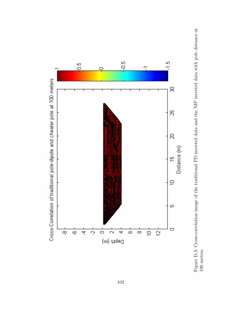
Fig

ure

D.3

:C

ross

-cor

rela

tion

imag

eof

the

trad

itio

nal

PD

inve

rted

dat

aan

dth

eN

IPin

vert

eddat

aw

ith

pol

edis

tance

at10

0m

etre

s.

102

Fig

ure

D.4

:C

ross

-cor

rela

tion

imag

eof

the

trad

itio

nal

PD

inve

rted

dat

aan

dth

eN

IPin

vert

eddat

aw

ith

pol

edis

tance

at50

met

res.

103

Fig

ure

D.5

:C

ross

-cor

rela

tion

imag

eof

the

trad

itio

nal

PD

inve

rted

dat

aan

dth

eN

IPin

vert

eddat

aw

ith

pol

edis

tance

at25

met

res.

104

Fig

ure

D.6

:C

ross

-cor

rela

tion

imag

eof

the

trad

itio

nal

PD

inve

rted

dat

aan

dth

eN

IPin

vert

eddat

aw

ith

pol

edis

tance

at10

met

res.

105

Fig

ure

D.7

:C

ross

-cor

rela

tion

imag

eof

the

trad

itio

nal

PD

inve

rted

dat

aan

dN

IPin

vert

eddat

aw

ith

pol

edis

tance

at1

met

re.

106

Appendix E

Inverted sections from COMSOL

modelling

107

Fig

ure

E.1

:T

radit

ional

PD

inve

rted

sect

ion

from

CO

MSO

Lm

odel

.T

he

infinit

ep

ole

islo

cate

d10

tim

esth

ear

ray

lengt

hor

at8.

700

kilom

etre

saw

ayfr

omth

esu

rvey

line.

108

Fig

ure

E.2

:N

IPin

vert

edse

ctio

nfr

omC

OM

SO

Lm

odel

wit

hp

ole

dis

tance

at4.

350

kilom

etre

sor

5ti

mes

the

arra

yle

ngt

h.

109

Fig

ure

E.3

:N

IPin

vert

edse

ctio

nfr

omC

OM

SO

Lm

odel

wit

hp

ole

dis

tance

at3.

480

kilom

etre

sor

4ti

mes

the

arra

yle

ngt

h.

110

Fig

ure

E.4

:N

IPin

vert

edse

ctio

nfr

omC

OM

SO

Lm

odel

wit

hp

ole

dis

tance

at2.

610

kilom

etre

sor

3ti

mes

the

arra

yle

ngt

h.

111

Fig

ure

E.5

:N

IPin

vert

edse

ctio

nfr

omC

OM

SO

Lm

odel

wit

hp

ole

dis

tance

at2.

175

kilom

etre

sor

2.5

tim

esth

ear

ray

lengt

h.

112

Fig

ure

E.6

:N

IPin

vert

edse

ctio

nfr

omC

OM

SO

Lm

odel

wit

hp

ole

dis

tance

at1.

740

kilom

etre

sor

2ti

mes

the

arra

yle

ngt

h.

113

Fig

ure

E.7

:N

IPin

vert

edse

ctio

nfr

omC

OM

SO

Lm

odel

wit

hp

ole

dis

tance

at1.

305

kilom

etre

sor

1.5

tim

esth

ear

ray

lengt

h.

114

Fig

ure

E.8

:N

IPin

vert

edse

ctio

nfr

omC

OM

SO

Lm

odel

wit

hp

ole

dis

tance

at87

0m

etre

sor

one

arra

yle

ngt

h.

115

Fig

ure

E.9

:N

IPin

vert

edse

ctio

nfr

omC

OM

SO

Lm

odel

wit

hp

ole

dis

tance

at30

met

res

oron

eel

ectr

ode

spac

ing

away

from

the

end

ofsu

rvey

line.

116

Appendix F

Sensitivity sections from COMSOL

modelling

117

Fig

ure

F.1

:Sen

siti

vit

yse

ctio

nca

lcula

ted

from

CO

MSO

Lm

odel

inve

rted

dat

a.T

he

top

sensi

tivit

yse

ctio

nis

from

the

trad

itio

nal

PD

.T

he

bot

tom

isa

NIP

PD

wit

hp

ole

dis

tance

at4.

350

kilom

etre

sor

5ti

mes

the

arra

yle

ngt

h.

118

Fig

ure

F.2

:Sen

siti

vit

yse

ctio

nca

lcula

ted

from

CO

MSO

Lm

odel

inve

rted

dat

a.T

he

top

sensi

tivit

yse

ctio

nis

from

the

trad

itio

nal

PD

.T

he

bot

tom

isa

NIP

PD

wit

hp

ole

dis

tance

at3.

480

kilom

etre

sor

4ti

mes

the

arra

yle

ngt

h.

119

Fig

ure

F.3

:Sen

siti

vit

yse

ctio

nca

lcula

ted

from

CO

MSO

Lm

odel

inve

rted

dat

a.T

he

top

sensi

tivit

yse

ctio

nis

from

the

trad

itio

nal

PD

.T

he

bot

tom

isa

NIP

PD

wit

hp

ole

dis

tance

at2.

610

kilom

etre

sor

3ti

mes

the

arra

yle

ngt

h.

120

Fig

ure

F.4

:Sen

siti

vit

yse

ctio

ns

calc

ula

ted

from

CO

MSO

Lm

odel

inve

rted

dat

a.T

he

top

sensi

tivit

yse

ctio

nis

calc

ula

ted

from

the

trad

itio

nal

PD

.T

he

bot

tom

sect

ion

isa

NIP

PD

wit

hp

ole

dis

tance

at2.

175

kilom

etre

sor

2.5

tim

esth

ear

ray

121

Fig

ure

F.5

:Sen

siti

vit

yse

ctio

nca

lcula

ted

from

CO

MSO

Lm

odel

inve

rted

dat

a.T

he

top

sensi

tivit

yse

ctio

nis

from

the

trad

itio

nal

PD

.T

he

bot

tom

isa

NIP

PD

wit

hp

ole

dis

tance

at1.

740

kilom

etre

sor

2ti

mes

the

arra

yle

ngt

h.

122

Fig

ure

F.6

:Sen

siti

vit

yse

ctio

ns

calc

ula

ted

from

CO

MSO

Lm

odel

inve

rted

dat

a.T

he

top

sensi

tivit

yse

ctio

nis

calc

ula

ted

from

the

trad

itio

nal

PD

.T

he

bot

tom

sect

ion

isa

NIP

PD

wit

hp

ole

dis

tance

at1.

305

met

res

or1.

5ti

mes

the

arra

y

123

Fig

ure

F.7

:Sen

siti

vit

yse

ctio

nca

lcula

ted

from

CO

MSO

Lm

odel

inve

rted

dat

a.T

he

top

sensi

tivit

yse

ctio

nis

from

the

trad

itio

nal

PD

.T

he

bot

tom

isa

NIP

PD

wit

hp

ole

dis

tance

at87

0m

etre

sor

one

arra

yle

ngt

h.

124

Fig

ure

F.8

:Sen

siti

vit

yse

ctio

ns

calc

ula

ted

from

CO

MSO

Lm

odel

inve

rted

dat

a.T

he

top

sensi

tivit

yse

ctio

nis

calc

ula

ted

from

the

trad

itio

nal

PD

.T

he

bot

tom

sect

ion

isa

NIP

PD

wit

hp

ole

dis

tance

at30

met

res

oron

eel

ectr

ode

spac

ing

from

the

end

ofth

ear

ray.

125

Appendix G

Cross-correlation sections from

COMSOL modelling

126

Fig

ure

G.1

:C

ross

-cor

rela

ted

sect

ion

mad

efr

omdat

ain

vers

ion

contr

ol.

This

sect

ion

was

cros

s-co

rrel

ated

usi

ng

the

trad

i-ti

onal

PD

dat

aco

mpute

dfr

omC

OM

SO

L.

The

trad

itio

nal

PD

dat

ase

tw

asin

vert

edtw

ice

inR

ES2D

INV

toob

tain

2se

tsof

dat

a.T

hes

e2

sets

ofdat

aar

eco

mpar

edto

them

selv

esfo

rsi

milar

itie

s.T

he

sim

ilar

itie

sar

ein

red

ora

scal

eof

one

and

the

diff

eren

ces

can

be

seen

inblu

e.A

lthou

ghth

e2

inve

rted

dat

ase

tsar

efr

omth

esa

me

forw

ard

dat

a,but

ther

ear

est

ill

diff

eren

ces

inth

eC

C.

This

isdue

toth

enon

-uniq

uen

ess

ofth

ein

vers

ion

pro

cess

.

127

Fig

ure

G.2

:C

ross

-cor

rela

ted

sect

ion

bet

wee

nin

vert

edtr

adit

ional

PD

dat

aan

dN

IPin

vert

eddat

aw

ith

pol

edis

tance

at4.

350

kilom

etre

sor

5ti

mes

the

arra

yle

ngt

h.

128

Fig

ure

G.3

:C

ross

-cor

rela

ted

sect

ion

bet

wee

nin

vert

edtr

adit

ional

PD

dat

aan

dN

IPin

vert

eddat

aw

ith

pol

edis

tance

at3.

480

kilom

etre

sor

4ti

mes

the

arra

yle

ngt

h.

129

Fig

ure

G.4

:C

ross

-cor

rela

ted

sect

ion

bet

wee

nin

vert

edtr

adit

ional

PD

dat

aan

dN

IPin

vert

eddat

aw

ith

pol

edis

tance

at2.

610

kilom

etre

sor

3ti

mes

the

arra

yle

ngt

h.

130

Fig

ure

G.5

:C

ross

-cor

rela

ted

sect

ion

bet

wee

nin

vert

edtr

adit

ional

PD

dat

aan

dN

IPin

vert

eddat

aw

ith

pol

edis

tance

at2.

175

kilom

etre

sor

2.5

tim

esth

ear

ray

lengt

h.

131

Fig

ure

G.6

:C

ross

-cor

rela

ted

sect

ion

bet

wee

nin

vert

edtr

adit

ional

PD

dat

aan

dN

IPin

vert

eddat

aw

ith

pol

edis

tance

at1.

740

kilom

etre

sor

2ti

mes

the

arra

yle

ngt

h.

132

Fig

ure

G.7

:C

ross

-cor

rela

ted

sect

ion

bet

wee

nin

vert

edtr

adit

ional

PD

dat

aan

dN

IPin

vert

eddat

aw

ith

pol

edis

tance

at1.

305

kilom

etre

sor

1.5

tim

esth

ear

ray

lengt

h.

133

Fig

ure

G.8

:C

ross

-cor

rela

ted

sect

ion

bet

wee

nin

vert

edtr

adit

ional

PD

dat

aan

dN

IPin

vert

eddat

aw

ith

pol

edis

tance

at87

0m

etre

sor

one

arra

yle

ngt

h.

134

Fig

ure

G.9

:C

ross

-cor

rela

ted

sect

ion

bet

wee

nin

vert

edtr

adit

ional

PD

dat

aan

dN

IPin

vert

eddat

aw

ith

pol

edis

tance

at30

met

res

oron

eel

ectr

ode

spac

ing

from

the

end

ofsu

rvey

line.

135

THE ELIMINATION OF THE INFINITE POLE IN THE POLE-DIPOLE ...

Documents

Transcript of THE ELIMINATION OF THE INFINITE POLE IN THE POLE-DIPOLE ...