The Electromagnetic Green’s Function for Layered Topological Insulators

J. A. Crosse,1, ∗ Sebastian Fuchs,2 and Stefan Yoshi Buhmann2, 3

1Department of Electrical and Computer Engineering,National University of Singapore, 4 Engineering Drive 3, Singapore 117583.

2Physikalisches Institut, Albert-Ludwigs-Universitat Freiburg,Hermann-Herder-Str. 3, 79104 Freiburg, Germany.

3Freiburg Institute for Advanced Studies, Albert-Ludwigs-Universitat Freiburg,Albertstraße 19, 79104 Freiburg, Germany.

(Dated: March 6, 2018)

The dyadic Green’s function of the inhomogeneous vector Helmholtz equation describes the fieldpattern of a single frequency point source. It appears in the mathematical description of many areasof electromagnetism and optics including both classical and quantum, linear and nonlinear optics,dispersion forces (such as the Casimir and Casimir-Polder forces) and in the dynamics of trappedatoms and molecules. Here, we compute the Green’s function for a layered topological insulator.Via the magnetoelectric effect, topological insulators are able to mix the electric, E, and magneticinduction, B, fields and, hence, one finds that the TE and TM polarizations mix on reflectionfrom/transmission through an interface. This leads to novel field patterns close to the surface of atopological insulator.

PACS numbers: 78.20.-e, 78.20.Ek, 78.67.Pt, 42.25.Gy

I. INTRODUCTION

Topological insulators are a class of time-reversal sym-metric materials that display non-trivial topological or-der and are characterized by an insulating bulk with pro-tected conducting edge states [1, 2]. This type of mate-rial was first predicted [3] and then observed [4] in 2Din HgTe/CdTe quantum wells and subsequently in 3Din Group V and Group V/VI alloys that display strongenough spin orbit coupling to induce band inversion -Bi1−xSbx in the first instance [5, 6] and then in Bi2Se3,Bi2Te3 and Sb2Te3 [7, 8] to name but a few examples.Owing to their unusual band structure, these materi-als display a number of unique electronic properties, themost notable of which is the quantum spin hall effectwhere quantized surface spin currents are observed eventhough the usual charge currents are absent [9, 10].

In addition to their interesting electronic properties,topological insulators also display a number of unusualelectromagnetic properties. Specifically, topological in-sulators have the ability to mix electric, E, and mag-netic induction, B, fields [11, 12], a feature which has apronounced affect on the optical response of the mate-rial [13–15]. In particular, this magnetoelectric E − Bmixing allows one to realise an axionic material [16, 17].Such materials are described by the Lagrangian densityL0 + Laxion, where L0 is the usual electromagnetic La-grangian density and Laxion is a term that couples theelectric and magnetic induction fields. This additionalelectromagnetic interaction reads

Laxion =α

4π2

Θ(r, ω)

µ0cE(r, ω) ·B(r, ω), (1)

∗Electronic address: alexcrosse@gmail.com

where α is the fine structure constant and Θ(r, ω) istermed the axion field in particle physics (although, asfar as electromagnetism is concerned, it merely acts asa space and frequency dependent coupling parameter).In order to realise such a material in a topological in-sulator, a time symmetry breaking perturbation of suffi-cient size must be introduced to the surface to induce agap, thereby converting the material into a full insulator.Such a gap can be opened by introducing ferromagneticdopants to the surface (12% Fe doping in Bi2Se3 leadsto a mid-infrared gap of 50meV/25µm [18]) or by theapplication of an external static magnetic field [19]. Insuch a time-reversal-symmetry-broken topological insula-tor (TSB-TI) the constitutive relations are altered and,hence, the optical properties of the material change dra-matically.

Here, we derive the electromagnetic Green’s functionfor a layered TSB-TI. The electromagnetic Green’s func-tion is the solution to the vector Helmholtz equation fora single frequency point source and can be used to gen-erate general field solutions for an arbitrary distributionof sources. This function has a wide range of applica-tions in both classical [20, 21] and quantum optics [22–25]and is an important component in studies of linear [26]and non-linear [27, 28] optics, Casimir [29] and Casmir-Polder [30, 31] forces, decoherence [32] and the dynam-ics of trapped atoms [33] and molecules [34, 35]. Thus,knowledge of the Green’s function is of value to a greatmany fields.

II. MAXWELL EQUATIONS

As with all electromagnetic studies, we begin with theMaxwell equations and constitutive relations for the ma-

arX

iv:1

509.

0301

2v1

[ph

ysic

s.op

tics]

10

Sep

2015

2

terial in question. For a TSB-TI these are [12, 13, 17]

∇ ·B(r, ω) = 0, (2)

∇×E(r, ω)− iωB(r, ω) = 0, (3)

∇ ·D(r, ω) = ρ(r, ω), (4)

∇×H(r, ω) + iωD(r, ω) = J(r, ω), (5)

and

D(r, ω) = ε0ε(r, ω)E(r, ω)

+α

π

Θ(r, ω)

µ0cB(r, ω) + PN (r, ω), (6)

H(r, ω) =1

µ0µ(r, ω)B(r, ω)

− α

π

Θ(r, ω)

µ0cE(r, ω)−MN (r, ω), (7)

where α is the fine structure constant and ε(r, ω), µ(r, ω)and Θ(r, ω) are the dielectric permittivity, magneticpermeability and axion coupling respectively, the lat-ter of which takes even multiples of π in a conventionalmagneto-dielectric and odd multiples of π in TSB-TI,with the magnitude and sign of the multiple given bythe strength and direction of the time symmetry break-ing perturbation. The PN (r, ω) and MN (r, ω) terms arethe noise polarization and magnetization, respectively.These terms are Langevin noise terms that model ab-sorption within the material [23]. These relations can bederived from the Lagrangian density in Eq. (1) [16]. Us-ing the above constitutive relations, one can show thatthe frequency components of the electric field obey theinhomogeneous Helmholtz equation

∇× 1

µ(r, ω)∇×E(r, ω)− ω2

c2ε(r, ω)E(r, ω)

− iωc

α

π[∇Θ(r, ω)×E(r, ω)]

= iωµ0 [JE(r, ω) + JN (r, ω)] , (8)

where JE(r, ω) is the source term for electromagneticwaves generated by external currents and JN (r, ω) =−iωPN (r, ω) + ∇ × MN (r, ω) is the source term forelectromagnetic waves generated by noise fluctuationswithin the material. If the axion coupling is homoge-neous, Θ(r, ω) = Θ(ω), then the last term on the left-hand side vanishes and one finds that the propagation ofthe electric field is the same as in a conventional magneto-dielectric. As a result, electromagnetic waves propagat-ing within a homogeneous TSB-TI retain there usualproperties - dispersion is linear, the phase and group ve-locities are proportional to the usual refractive index, thefields are transverse and orthogonal polarizations do notmix. Thus, the effects of the axion coupling are only feltwhen the axion coupling varies in space. For layered, ho-mogeneous media this will occur only at the interfaceswhere the properties of the medium change.

III. FRESNEL COEFFICIENTS

An important set of functions for any layered mediaare the Fresnel coefficients for reflection and transmis-sion at each interface. These functions are required toconstruct the Green’s function. In fact, the Fresnel co-efficients for TSB-TIs have been studied before [13, 17],however, the standard expression for the Green’s functionrequires a slightly different form for the coefficients com-pared to those in previous work [20, 24]. Furthermore,certain aspects of TSB-TIs mean that the usual methodof computing this form of the coefficients leads to incor-rect results. For these reasons, it is worth revisiting thederivation in some detail.

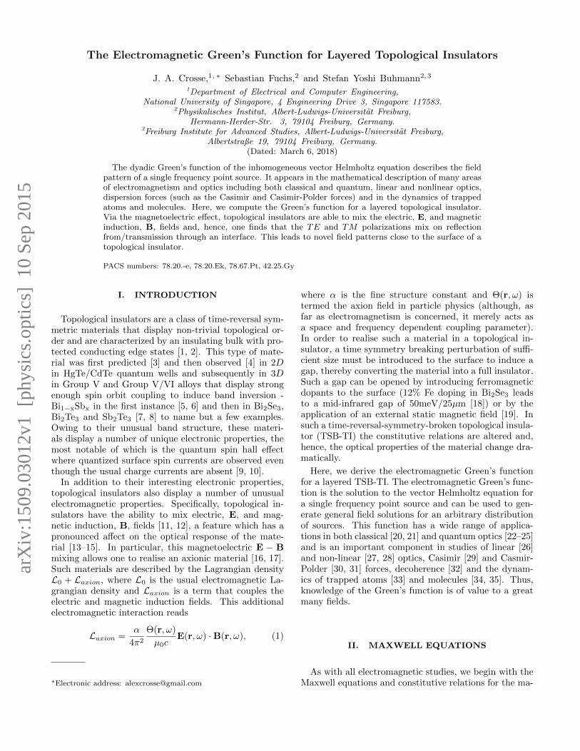
In the derivation of the Fresnel coefficients for a con-ventional magneto-dielectric one usually defines two po-larizations; the TE polarization, where the electric field,E, is parallel to the interface, and the TM polarization,where the magnetic field, H, is parallel to the interface.Since, from Eq. (8), the electric field propagation is unaf-fected by a homogeneous axion coupling one can see thatthe TE polarization is unchanged. However, from Eq.(7), one can see that the magnetic field, H, is no longerperpendicular to the electric field, E. Thus defining theTM polarization in terms of the magnetic field, H, leadsto two polarizations that are not orthogonal and henceincorrect expressions for the Fresnel coefficients. Fur-thermore, we would expect the two polarizations to mixat the interface via the magnetoelectric coupling, hencedefining the two polarizations in terms of different fieldsleads to awkward expressions. The simplest approach isto work solely with the electric field, E. Thus, for medialayered in the z direction and light incident in the x− zplane, we define the TE polarization as the polarizationwith Ey 6= 0 and Ex = 0, Ez = 0 and the TM polariza-tion as the polarization with Ey = 0 and Ex 6= 0, Ez 6= 0,[See Fig. 1].

We proceed by considering waves of a specific (TE,TM) polarization incident on an interface between twohomogeneous isotropic TSB-TIs. By matching the waves

z=0

z

x

Layer 1

Layer 2

ε1 μ1

ε2 μ2

Θ1

Θ2

TE PolarizedElectric Field

TM PolarizedElectric Field

ϕt

ϕrϕi

FIG. 1: The interface between two topological insulators.

3

in each half-space using the electromagnetic jump condi-tions

z ×E1 = z ×E2, (9)

z ×H1 = z ×H2, (10)

which relate the transverse components of the electricand magnetic fields on either side of the interface, theFresnel coefficients can be found.

First we consider a TE polarized plane wave incidenton the interface from layer 1 [See Fig. 1]. The electricfield ansatz for each region is

Ex,1 = −E0kz,1k1

eikz,1z+ikpxRTM,TE , (11)

Ey,1 = −E0

[e−ikz,1z+ikpx + eikz,1z+ikpxRTE,TE

], (12)

Ez,1 = E0kpk1eikz,1z+ikpxRTM,TE , (13)

Ex,2 = E0kz,2k2

e−ikz,2z+ikpxTTM,TE , (14)

Ey,2 = −E0e−ikz,2z+ikpxTTE,TE , (15)

Ez,2 = E0kpk2e−ikz,2z+ikpxTTM,TE , (16)

where the kz/k1 = cosφr, kp/k1 = sinφr, kz/k2 = cosφt,kp/k2 = sinφt. It has been previously shown that Snell’slaw holds for TSB-TI’s so φi = φr [13, 17]. From Eqs.(3) and (7) we obtain

Hx,1 = −E0kz,1µ0µ1ω

[e−ikz,1z+ikpx − eikz,1z+ikpxRTE,TE

]+ E0

α

π

Θ1

µ0c

kz,1k1

eikz,1z+ikpxRTM,TE , (17)

Hy,1 = −E0k1

µ0µ1ωeikz,1z+ikpxRTM,TE

+ E0α

π

Θ1

µ0c

[e−ikz,1z+ikpx + eikz,1z+ikpxRTE,TE

],

(18)

Hx,2 = −E0kz,2µ0µ2ω

e−ikz,1z+ikpxTTE,TE

− E0α

π

Θ2

µ0c

kz,2k2

e−ikz,1z+ikpxTTM,TE , (19)

Hy,2 = −E0k2

µ0µ2ωe−ikz,1z+ikpxTTM,TE

+ E0α

π

Θ2

µ0ce−ikz,1z+ikpxTTE,TE . (20)

From Eqs. (9) and (10) we can find the boundary condi-

tions for the fields at the interface at z = 0

1 +RTE,TE = TTE,TE , (21)

−kz,1n1

RTM,TE =kz,2n2

TTM,TE , (22)

−kz,1µ1

[1−RTE,TE ] +α

πΘ1

kz,1n1

RTM,TE

= −kz,2µ2

TTE,TE −α

πΘ2

kz,2n2

TTM,TE , (23)

n1µ1RTM,TE −

α

πΘ1 [1 +RTE,TE ]

=n2µ2TTM,TE −

α

πΘ2TTE,TE , (24)

where we have used the dispersion relation k = nω/c.Solving the above system of equations gives

RTE,TE =(µ2kz,1 − µ1kz,2)Ωε − kz,1kz,2∆2

(µ2kz,1 + µ1kz,2)Ωε + kz,1kz,2∆2, (25)

RTM,TE =−2µ2n1kz,1kz,2∆

(µ2kz,1 + µ1kz,2)Ωε + kz,1kz,2∆2, (26)

TTE,TE =2µ2kz,1Ωε

(µ2kz,1 + µ1kz,2)Ωε + kz,1kz,2∆2, (27)

TTM,TE =2µ2n2k

2z,1∆

(µ2kz,1 + µ1kz,2)Ωε + kz,1kz,2∆2, (28)

where ∆ = αµ1µ2(Θ2 − Θ1)/π and Ωε = µ1µ2(kz,1ε2 +kz,2ε1), with the factors of ε appearing via the defi-nition of the refractive index, n2 = µε. Note thatwhen Θ2 − Θ1 → 0 (i.e when the axion couplings van-ish or when they are the same across the interface),RTM,TE , TTM,TE → 0 and RTE,TE and TTE,TE reduceto the usual reflection coefficients for normal magneto-electric materials [20, 24].

Next, we consider a TM polarized plane wave incidenton the interface from layer 1 [See Fig. 1]. The electricfield ansatz for each region is now

Ex,1 = E0kz,1k1

[e−ikz,1z+ikpx − eikz,1z+ikpxRTM,TM

],

(29)

Ey,1 = −E0eikz,1z+ikpxRTE,TM , (30)

Ez,1 = E0kpk1

[e−ikz,1z+ikpx + eikz,1z+ikpxRTM,TM

],

(31)

Ex,2 = E0kz,2k2

e−ikz,2z+ikpxTTM,TM , (32)

Ey,2 = −E0e−ikz,2z+ikpxTTE,TM , (33)

Ez,2 = E0kpk2e−ikz,2z+ikpxTTM,TM , (34)

where, again, components of the wavenumber are relatedto the angles of incidence, reflection and transmission and

4

Snells law holds. From Eqs. (3) and Eq. (7) we obtain

Hx,1 = E0kz,1µ0µ1ω

eikz,1z+ikpxRTE,TM

− E0α

π

Θ1

µ0c

kz,1k1

[e−ikz,1z+ikpx − eikz,1z+ikpxRTM,TM

],

(35)

Hy,1 = −E0k1

µ0µ1ω

[e−ikz,1z+ikpx + eikz,1z+ikpxRTM,TM

]+ E0

α

π

Θ1

µ0ceikz,1z+ikpxRTE,TM , (36)

Hx,2 = −E0kz,2µ0µ2ω

e−ikz,2z+ikpxTTE,TM

− E0α

π

Θ2

µ0c

kz,2k2

e−ikz,2z+ikpxTTM,TM , (37)

Hy,2 = −E0k2

µ0µ2ωe−ikz,2z+ikpxTTM,TM

+ E0α

π

Θ2

µ0ce−ikz,2z+ikpxTTE,TM . (38)

From Eqs. (9) and (10) we can, again, find the boundaryconditions for the fields at the interface at z = 0

kz,1n1

[1−RTM,TM ] =kz,2n2

TTM,TM , (39)

RTE,TM = TTE,TM , (40)

kz,1µ1

RTE,TM −α

πΘ1

kz,1n1

[1−RTM,TM ]

= −kz,2µ2

TTE,TM −α

πΘ2

kz,2n2

TTM,TM , (41)

n1µ1

[1 +RTM,TM ]− α

πΘ1RTE,TM

=n2µ2TTM,TM −

α

πΘ2TTE,TM , (42)

where, once more, k = nω/c has been used. Solving theabove system of equations gives

RTM,TM =(ε2kz,1 − ε1kz,2)Ωµ + kz,1kz,2∆2

(ε2kz,1 + ε1kz,2)Ωµ + kz,1kz,2∆2, (43)

RTE,TM =−2µ2n1kz,1kz,2∆

(ε2kz,1 + ε1kz,2)Ωµ + kz,1kz,2∆2, (44)

TTM,TM =n2n1

2ε1kz,1Ωµ(ε2kz,1 + ε1kz,2)Ωµ + kz,1kz,2∆2

, (45)

TTE,TM =−2µ2n1kz,1kz,2∆

(ε2kz,1 + ε1kz,2)Ωµ + kz,1kz,2∆2, (46)

where ∆ = αµ1µ2(Θ2 − Θ1)/π and Ωµ = µ1µ2(kz,1µ2 +kz,2µ1), with the factors of ε, again, appearing via thedefinition of the refractive index. Once again, whenΘ2 − Θ1 → 0 (i.e when the axion couplings van-ish or when they are the same across the interface),RTE,TM , TTE,TM → 0 and RTM,TM and TTM,TM reduceto the usual reflection coefficients for normal magneto-electric materials [20, 24]. (Note that in [20], unlike [24],

the transmission coefficient differs from the above resultby the ratio of the impedances of the two layers. This isbecause the TM coefficients are derived using the H-fieldinstead of the E-field.)

The Fresnel coefficients for the energy flux can befound by comparing the z-component of the Poyntingvector, S = E × H, on each side of the interface. Onefinds that they are related to the above field coefficientsvia

ri,j = |Ri,j |2, (47)

ti,j =kz,2kz,1

µ1

µ2|Ti,j |2, (48)

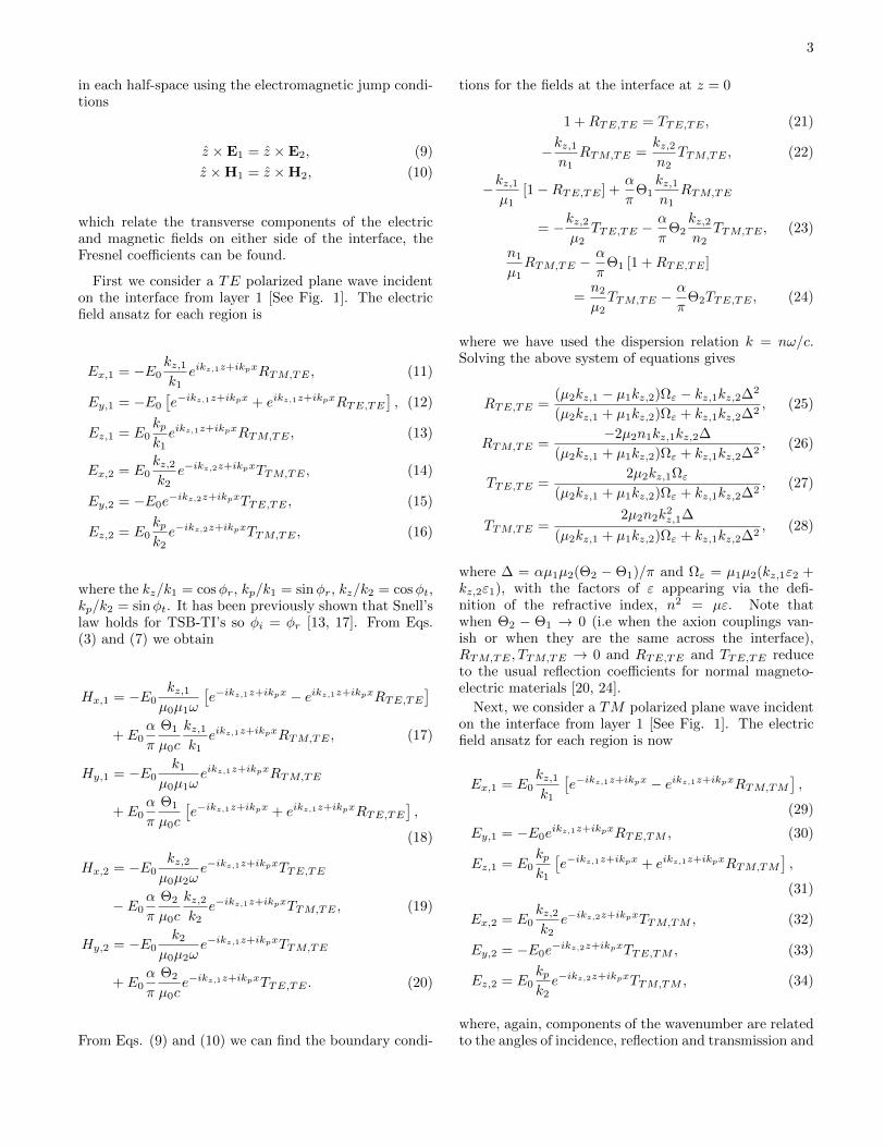
where i, j ∈ TE, TM and the prefactor in the transmis-sion coefficients accounting for the change in flux areaas the field passes through the interface. Figure 2 showsthe reflection, ri,i, and transmission, ti,i, as a function ofincident angle for a 600nm optical plane wave, incidentfrom the vacuum, encountering a conventional magneto-dielectric with ε = 16 and µ = 1 (such values are simi-lar to those for Bi2Se3 at high frequencies [36]). In this

Angle of Incidence ϕ ( )oi

Refl

ectio

n/Tr

ansm

issi

on (%

)

20 40 60 80

20

40

60

80

100

FIG. 2: (Color online) The % reflection (solid) and transmis-sion (dashed) for TE (red) and TM (blue) polarized waves ata vacuum- (layer 1) magneto-dielectic- (layer 2) interface as afunction of the incident angle, φi. Here, µ1 = µ2 = 1, ε1 = 1and ε2 = 16.

case the mixing coefficients vanish and the polarizationstate of the incident light is preserved by the interface.It is easy to see that for incident TE polarized lightrTE,TE + tTE,TE = 1 hence the TE energy flux is pre-served at the interface (a similar expression holds for TMpolarized light). In comparison, Fig. 3 shows the reflec-tion, ri,i, transmission, ti,i, and mixing, ri,j/ti,j (i 6= j),as a function of incident angle for a plane wave of simi-lar wavelength, incident from the vacuum, encounteringa TSB-TI with ε = 16, µ = 1 and Θ2 = π. In thiscase the mixing coefficients are non-zero and the polar-ization states of the incident light mix at the interface.Finally, one can show that for incident TE polarized

5

Angle of Incidence ϕ ( )oi

Refl

ectio

n/Tr

ansm

issi

on (%

)

Angle of Incidence ϕ ( )oi

(a)

(b)

Refl

ectio

n/Tr

ansm

issi

on (x

10

%)

-5

20 40 60 80

20

40

60

80

100

20 40 60 80

10

20

30

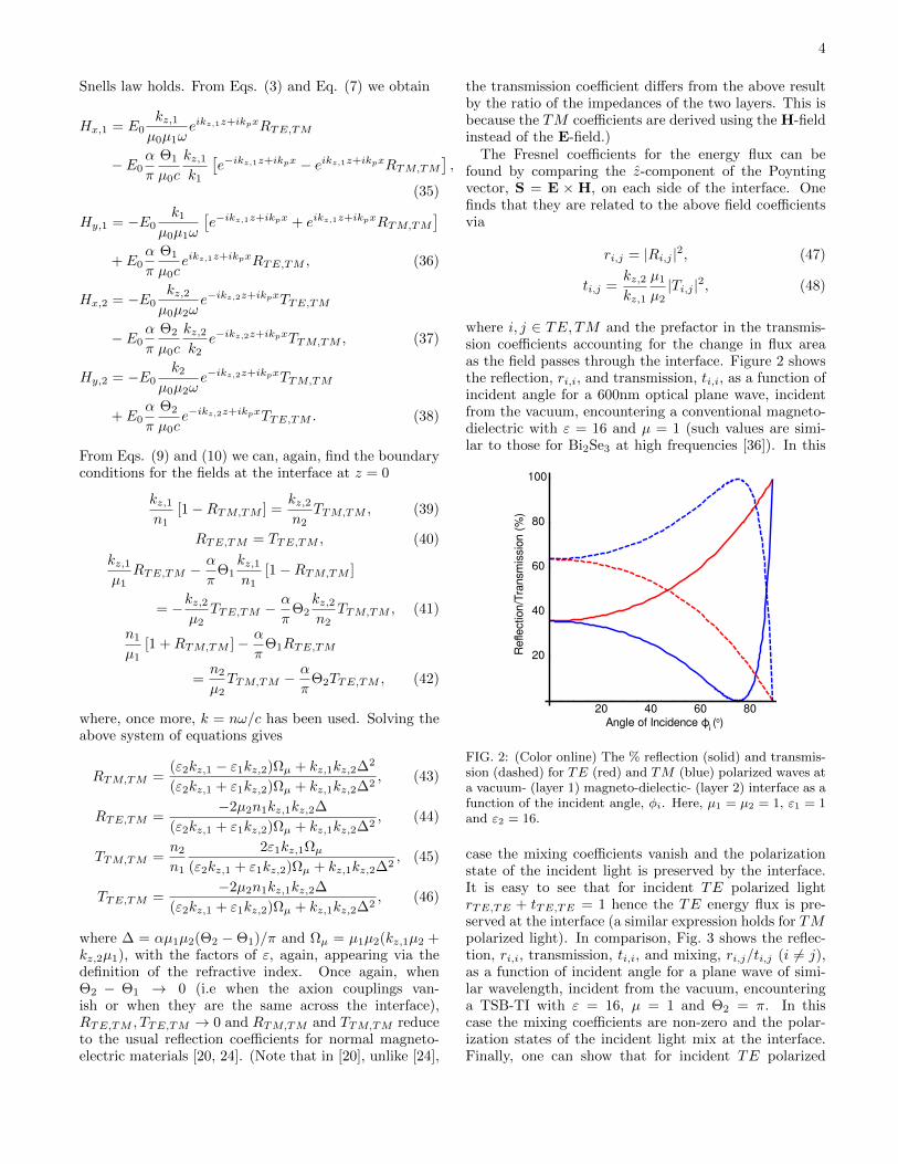
FIG. 3: (Color online) (a) The % reflection (solid) and trans-mission (dashed) for TE (red) and TM (blue) polarized wavesat a vacuum- (layer 1) TRSB-TI- (layer 2) interface as a func-tion of the incident angle, φi. (b) The % reflection (solid)and transmission (dashed) for TE → TM mixing (red) andTM → TE mixing (blue) at a vacuum- (layer 1) TRSB-TI-(layer 2) interface as a function of the incident angle, φi. Inboth cases, µ1 = µ2 = 1, ε1 = 1, ε2 = 16, Θ1 = 0 and Θ2 = π.

light, rTE,TE + rTM,TE + tTE,TE + tTM,TE = 1 henceTE energy flux is still preserved at the interface (againa similar expression holds for TM polarized light).

In order to better understand the mixing coefficients,it is informative to look at the case of a pure TSB-TIwhere the permittivity and permeability are that of thevacuum and only the axion coupling changes on the in-terface. This allows one to remove the magneto-dielectriceffects from the system and isolate the effect of the axioncoupling. In this case kz,1 = kz,2 and the reflection andtransmission coefficients reduce to

RTE,TE = −RTM,TM =−∆2

4 + ∆2, (49)

TTE,TE = TTM,TM =4

4 + ∆2, (50)

RTM,TE = RTE,TM = −TTM,TE = TTE,TM =−2∆

4 + ∆2.

(51)

(Similar expressions were found in [17].) One can seethat in the pure TSB-TI limit the reflection and trans-mission coefficients are no longer a function of incidentangle and, hence, the angular dependence of the coef-ficients is a result of the magneto-dielectric propertiesof the material rather than the axionic properties. As∆ ≈ α, the energy flux reflection and transmission coeffi-cients are ri,i ≈ α4/16 ≈ 10−10 and ti,i ≈ 1 respectively.Thus one sees near perfect transmission. However, sincethe axion coupling changes on the interface one still hasmixing, the magnitude of which is equal in transmissionand reflection ri,j = ti,j ≈ α2/4 ≈ 10−5.

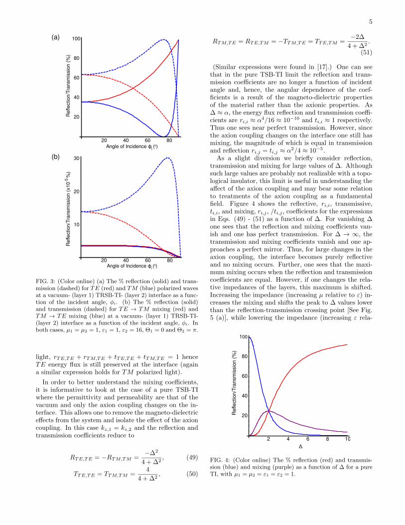
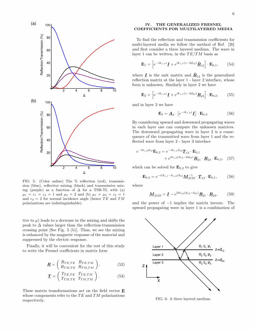
As a slight diversion we briefly consider reflection,transmission and mixing for large values of ∆. Althoughsuch large values are probably not realizable with a topo-logical insulator, this limit is useful in understanding theaffect of the axion coupling and may bear some relationto treatments of the axion coupling as a fundamentalfield. Figure 4 shows the reflective, ri,i, transmissive,ti,i, and mixing, ri,j , /ti,j , coefficients for the expressionsin Eqs. (49) - (51) as a function of ∆. For vanishing ∆one sees that the reflection and mixing coefficients van-ish and one has perfect transmission. For ∆ → ∞, thetransmission and mixing coefficients vanish and one ap-proaches a perfect mirror. Thus, for large changes in theaxion coupling, the interface becomes purely reflectiveand no mixing occurs. Further, one sees that the maxi-mum mixing occurs when the reflection and transmissioncoefficients are equal. However, if one changes the rela-tive impedances of the layers, this maximum is shifted.Increasing the impedance (increasing µ relative to ε) in-creases the mixing and shifts the peak to ∆ values lowerthan the reflection-transmission crossing point [See Fig.5 (a)], while lowering the impedance (increasing ε rela-

2 4 6 8 10

20

40

60

80

100

Δ

Refl

ectio

n/Tr

ansm

issi

on (%

)

FIG. 4: (Color online) The % reflection (red) and transmis-sion (blue) and mixing (purple) as a function of ∆ for a pureTI, with µ1 = µ2 = ε1 = ε2 = 1.

6

(a)

(b)

2 4 6 8 10

20

40

60

80

100

Δ

Refl

ectio

n/Tr

ansm

issi

on (%

)

2 4 6 8 10

20

40

60

80

100

Δ

Refl

ectio

n/Tr

ansm

issi

on (%

)

FIG. 5: (Color online) The % reflection (red), transmis-sion (blue), reflective mixing (black) and transmissive mix-ing (purple) as a function of ∆ for a TSB-TI, with (a)µ1 = ε1 = ε2 = 1 and µ2 = 2 and (b) µ1 = µ2 = ε2 = 1and ε2 = 2 for normal incidence angle (hence TE and TMpolarizations are indistinguishable).

tive to µ) leads to a decrease in the mixing and shifts thepeak to ∆ values larger than the reflection-transmissioncrossing point [See Fig. 5 (b)]. Thus, we see the mixingis enhanced by the magnetic response of the material andsuppressed by the electric response.

Finally, it will be convenient for the rest of this studyto write the Fresnel coefficients in matrix form

R =

(RTE,TE RTE,TMRTM,TE RTM,TM

), (52)

T =

(TTE,TE TTE,TMTTM,TE TTM,TM

). (53)

These matrix transformations act on the field vector Ewhose components refer to the TE and TM polarizationsrespectively.

IV. THE GENERALIZED FRESNELCOEFFICIENTS FOR MULTILAYERED MEDIA

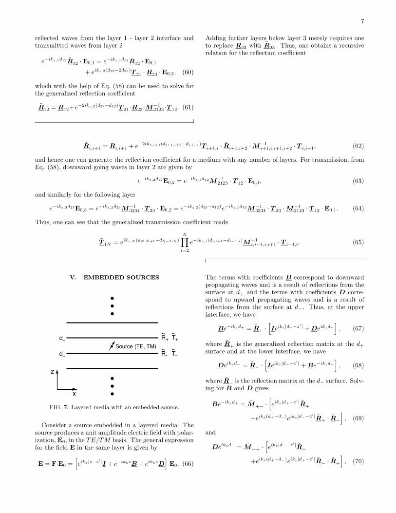
To find the reflection and transmission coefficients formulti-layered media we follow the method of Ref. [20]and first consider a three layered medium. The wave inlayer 1 can be written, in the TE/TM basis as

E1 =[e−ikz,1zI + eikz,1(z−2d12)R12

]·E0,1, (54)

where I is the unit matrix and R12 is the generalizedreflection matrix at the layer 1 - layer 2 interface, whoseform is unknown. Similarly in layer 2 we have

E2 =[e−ikz,2zI + eikz,1(z−2d23)R23

]·E0,2, (55)

and in layer 3 we have

E3 = A3 ·[e−ikz,3zI

]·E0,3. (56)

By considering upward and downward propagating wavesin each layer one can compute the unknown matrices.The downward propagating wave in layer 2 is a conse-quence of the transmitted wave from layer 1 and the re-flected wave from layer 2 - layer 3 interface

e−ikz,2d12E0,2 = e−ikz,1d12T 12 ·E0,1

+ eikz,2(d12−2d23)R21 ·R23 ·E0,2, (57)

which can be solved for E0,2 to give

E0,2 = e−i(kz,1−kz,2)d12M−12123 · T 12 ·E0,1, (58)

where

M2123 = I − e2ikz2(d12−d23)R21 ·R23, (59)

and the power of −1 implies the matrix inverse. Theupward propagating wave in layer 1 is a combination of

z=d

z

x

Layer 1

Layer 2

ε1 μ1

ε2 μ2

Θ1

Θ2

Layer 3 ε3 μ3Θ3z=d

12

23

FIG. 6: A three layered medium.

7

reflected waves from the layer 1 - layer 2 interface andtransmitted waves from layer 2

e−ikz,1d12R12 ·E0,1 = e−ikz,1d12R12 ·E0,1

+ eikz,2(d12−2d23)T 21 ·R23 ·E0,2, (60)

which with the help of Eq. (58) can be used to solve forthe generalized reflection coefficient

R12 = R12+e−2ikz,2(d23−d12)T 21 ·R23 ·M−12123 ·T 12. (61)

Adding further layers below layer 3 merely requires oneto replace R23 with R23. Thus, one obtains a recursiverelation for the reflection coefficient

Ri,i+1 = Ri,i+1 + e−2ikz,i+1(di+1,i+2−di,i+1)T i+1,i · Ri+1,i+2 ·M−1i+1,i,i+1,i+2 · T i,i+1, (62)

and hence one can generate the reflection coefficient for a medium with any number of layers. For transmission, fromEq. (58), downward going waves in layer 2 are given by

e−ikz,2d12E0,2 = e−ikz,1d12M−12123 · T 12 ·E0,1, (63)

and similarly for the following layer

e−ikz,3d23E0,3 = e−ikz,2d23M−13234 · T 23 ·E0,2 = e−ikz,2(d23−d12)e−ikz,1d12M−1

3234 · T 23 ·M−12123 · T 12 ·E0,1. (64)

Thus, one can see that the generalized transmission coefficient reads

T 1N = eikz,N (dN,N+1−dN−1,N )N∏i=2

e−ikz,i(di,i+1−di−1,i)M−1i,i−1,i,i+1 · T i−1,i. (65)

V. EMBEDDED SOURCES

Source (TE, TM)d

z

x

+

d-

R+ T+~ ~

R- T-~ ~

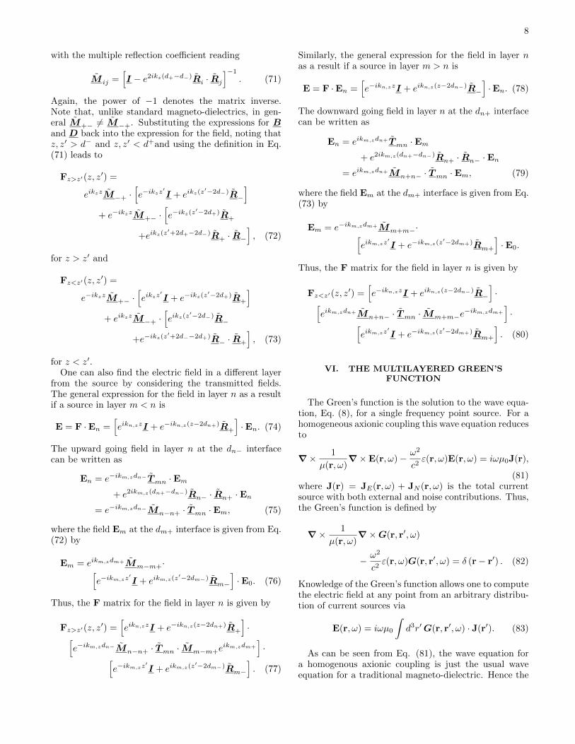
FIG. 7: Layered media with an embedded source.

Consider a source embedded in a layered media. Thesource produces a unit amplitude electric field with polar-ization, E0, in the TE/TM basis. The general expressionfor the field E in the same layer is given by

E = F·E0 =[eikz|z−z

′|I + e−ikzzB + eikzzD]·E0. (66)

The terms with coefficients B correspond to downwardpropagating waves and is a result of reflections from thesurface at d+ and the terms with coefficients D corre-spond to upward propagating waves and is a result ofreflections from the surface at d−. Thus, at the upperinterface, we have

Be−ikzd+ = R+ ·[Ieikz|d+−z

′| + Deikzd+], (67)

where R+ is the generalized reflection matrix at the d+surface and at the lower interface, we have

Deikzd− = R− ·[Ieikz|d−−z

′| + Be−ikzd−], (68)

where R− is the reflection matrix at the d− surface. Solv-ing for B and D gives

Be−ikzd+ = M+− ·[eikz|d+−z

′|R+

+eikz(d+−d−)eikz|d−−z′|R+ · R−

], (69)

and

Deikzd− = M−+ ·[eikz|d−−z

′|R−

+eikz(d+−d−)eikz|d+−z′|R− · R+

], (70)

8

with the multiple reflection coefficient reading

M ij =[I − e2ikz(d+−d−)Ri · Rj

]−1. (71)

Again, the power of −1 denotes the matrix inverse.Note that, unlike standard magneto-dielectrics, in gen-eral M+− 6= M−+. Substituting the expressions for Band D back into the expression for the field, noting thatz, z′ > d− and z, z′ < d+and using the definition in Eq.(71) leads to

Fz>z′(z, z′) =

eikzzM−+ ·[e−ikzz

′I + eikz(z

′−2d−)R−

]+ e−ikzzM+− ·

[e−ikz(z

′−2d+)R+

+eikz(z′+2d+−2d−)R+ · R−

], (72)

for z > z′ and

Fz<z′(z, z′) =

e−ikzzM+− ·[eikzz

′I + e−ikz(z

′−2d+)R+

]+ eikzzM−+ ·

[eikz(z

′−2d−)R−

+e−ikz(z′+2d−−2d+)R− · R+

], (73)

for z < z′.One can also find the electric field in a different layer

from the source by considering the transmitted fields.The general expression for the field in layer n as a resultif a source in layer m < n is

E = F ·En =[eikn,zzI + e−ikn,z(z−2dn+)R+

]·En. (74)

The upward going field in layer n at the dn− interfacecan be written as

En = e−ikm,zdn− Tmn ·Em+ e2ikm,z(dn+−dn−)Rn− · Rn+ ·En

= e−ikm,zdn−Mn−n+ · Tmn ·Em, (75)

where the field Em at the dm+ interface is given from Eq.(72) by

Em = eikm,zdm+Mm−m+·[e−ikm,zz

′I + eikm,z(z

′−2dm−)Rm−

]·E0. (76)

Thus, the F matrix for the field in layer n is given by

Fz>z′(z, z′) =

[eikn,zzI + e−ikn,z(z−2dn+)R+

]·[

e−ikm,zdn−Mn−n+ · Tmn · Mm−m+eikm,zdm+

]·[

e−ikm,zz′I + eikm,z(z

′−2dm−)Rm−

]. (77)

Similarly, the general expression for the field in layer nas a result if a source in layer m > n is

E = F ·En =[e−ikn,zzI + eikn,z(z−2dn−)R−

]·En. (78)

The downward going field in layer n at the dn+ interfacecan be written as

En = eikm,zdn+ Tmn ·Em+ e2ikm,z(dn+−dn−)Rn+ · Rn− ·En

= eikm,zdn+Mn+n− · Tmn ·Em, (79)

where the field Em at the dm+ interface is given from Eq.(73) by

Em = e−ikm,zdm+Mm+m−·[eikm,zz

′I + e−ikm,z(z

′−2dm+)Rm+

]·E0.

Thus, the F matrix for the field in layer n is given by

Fz<z′(z, z′) =

[e−ikn,zzI + eikn,z(z−2dn−)R−

]·[

eikm,zdn+Mn+n− · Tmn · Mm+m−e−ikm,zdm+

]·[

eikm,zz′I + e−ikm,z(z

′−2dm+)Rm+

]. (80)

VI. THE MULTILAYERED GREEN’SFUNCTION

The Green’s function is the solution to the wave equa-tion, Eq. (8), for a single frequency point source. For ahomogeneous axionic coupling this wave equation reducesto

∇× 1

µ(r, ω)∇×E(r, ω)− ω2

c2ε(r, ω)E(r, ω) = iωµ0J(r),

(81)where J(r) = JE(r, ω) + JN (r, ω) is the total currentsource with both external and noise contributions. Thus,the Green’s function is defined by

∇× 1

µ(r, ω)∇×G(r, r′, ω)

− ω2

c2ε(r, ω)G(r, r′, ω) = δ (r− r′) . (82)

Knowledge of the Green’s function allows one to computethe electric field at any point from an arbitrary distribu-tion of current sources via

E(r, ω) = iωµ0

∫d3r′G(r, r′, ω) · J(r′). (83)

As can be seen from Eq. (81), the wave equation fora homogenous axionic coupling is just the usual waveequation for a traditional magneto-dielectric. Hence the

9

Green’s function is identical to the standard magneto-dielectric electric Green’s function, which, in its singu-larity extracted form, reads

G(r, r′, ω) =i

8π2

∫d2kp µ(r′)

[m∗(r)⊗m(r′)

kzk2p

+n∗(r)⊗ n(r′)

kzk2p

]eikp·(rp−r′p)eikz|z−z

′|, (84)

where m(r) and n(r) are the dyadic operators

m(r) = i∇r × z, (85)

n(r) =1

k∇r ×∇r × z, (86)

that generate the solenoidal vector wave functions [20],which are equivalent to the polarization vectors in [24].Here, k is the wavevector of the wave with kp = kxx+ky y

and kz =√k2 − k2p. Similarly, rp = rxx + ry y. For

simplicity we have neglected the source singularity.The effect of the axionic coupling is only seen when

there are inhomogeneities in the material. Adding planarlayers is identical to finding generalized reflection coeffi-cients except now we replace the source E0 with a vectorcontaining the dyads. Thus the Green’s function for lay-ered TSB-TI’s is given by

Gz≷z′(r, r′, ω) =

i

8π2

∫d2kp

× µ(r′)

[C(r, r′) : F z≷z′(z, z

′)

kzk2p

]eikp·(rp−r′p), (87)

with

C(r, r′) =

(m∗(r)⊗m(r′) n∗(r)⊗m(r′)m∗(r)⊗ n(r′) n∗(r)⊗ n(r′)

), (88)

and the : operator implying the element-wise Frobeniusinner product. For z and z′ in the same layer F z>z′(z, z

′)is given by Eq. (72) and F z<z′(z, z

′) by Eq. (73). Forz ∈ n and z′ ∈ m in the different layers F z>z′(z, z

′)is given by Eq. (77) and F z<z′(z, z

′) by Eq. (80).As a consistency check, one can show that the result-ing Green’s function reduces to that for a traditionalmagneto-dielectric material when the axion coupling van-ishes and that it satisfies the Schwarz reflection principle,which is required for the response to be causal (see Ap-pendix A).

VII. DIPOLE FIELDS CLOSE TO A TSB-TISURFACE

As an example of the use of the Green’s function we willcompute the electric field pattern of a single frequency,dipole point source close to a TSB-TI surface at z = 0.We take the source to be in the upper layer, z′ > 0.

For a field point at z > 0 there are two contributions,one from direct propagation from the source to the fieldpoint, which is given by the free space Green’s functionG0(r, r′, ω), and one from reflections from the surface,which is given by the reflective part of the Green’s func-tion R(r, r′, ω). For z < 0 the only contribution is fromtransmission at the surface, which is given by the trans-missive part of the Greens function T (r, r′, ω). Thus, wecan split the Green’s function into 3 parts

G(r, r′, ω) =

G0(r, r′, ω) + R(r, r′, ω) z > 0,

T (r, r′, ω) z < 0,(89)

each of which can be computed separately. Each partcan be found by expanding the definition of the Green’sfunction given in Eq. (87). These expressions are givenin Appendix B.

A. z-Orientated-Dipole

First we will consider a single frequency, dipole pointsource, orientated in the z direction, placed close to amaterial surface. This source can be represented by acurrent density of the form

J(r′) = −iωd(ω)δ(r′)z, (90)

where d(ω) is the dipole strength. The source is placed inthe upper layer, which is taken to be the vacuum (ε = 1and µ = 1), at 1.5λ0 above a surface, where λ0 is thevacuum wavelength. The material parameters for thesurface are ε = 16 and µ = 1, which are comparable tothose of Bi2Se3 [36]. Substituting the current source intothe expression for the electric field in Eq. (83) shows thatthe relevant components of the Green’s function are theGiz(r, r′, ω), where i = x, y, z depending on the desiredfield component at r. The expression for the Green’sfunction components can be simplified by converting topolar coordinates, after which the angular integral can beperformed analytically. The resulting Hankel transformintegral, however, must be computed numerically (therelevant integrals can be found in Appendix C).

The field patterns for this configuration are shown inFigure 8. Figures 8 (a), (b) and (c) show the, x, y and zcomponents, respectively, for the real part of the electricfield (equivalent to the time dependent field at t = 0) inthe x − z plane for Θ = 0 - the case of a conventionalmagneto-dielectric. In this case the mixing coefficientsvanish and hence one sees y-component of the field iszero. The field patterns for the x and z components arethose that one would expect from a point dipole. Fig-ures 8 (d), (e) and (f) show the, x, y and z components,respectively, for the real part of the electric field in thex − z plane for the case of a TSB-TI with, Θ = π. Inthis case the mixing coefficients are non-zero. The axioncoupling causes a rotation of the polarization of the field,generating a non-zero y-component at the interface. Fig-ures 8 (g), (h) and (i) show the, x, y and z components,

10

z(λ

) 0

x(λ )0 x(λ )0 x(λ )0

z(λ

) 0

z(λ

) 0

z(λ

) 0

x(λ )0 x(λ )0 x(λ )0

z(λ

) 0

z(λ

) 0

z(λ

) 0

x(λ )0 x(λ )0 x(λ )0

z(λ

) 0

z(λ

) 0

(a) (b) (c)

(d) (e) (f)

(g) (h) (i)

x1000x1 x1

x1000x1 x1

x1000x1 x1

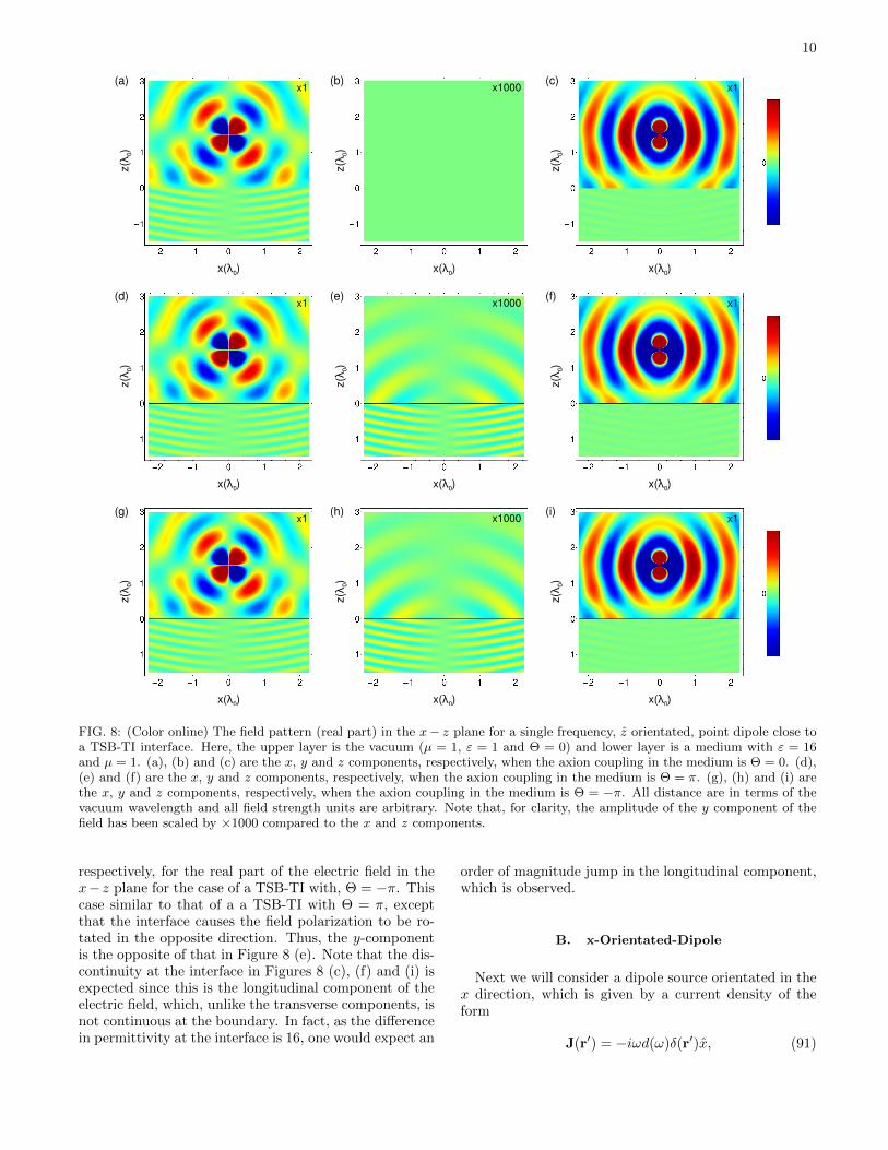
FIG. 8: (Color online) The field pattern (real part) in the x− z plane for a single frequency, z orientated, point dipole close toa TSB-TI interface. Here, the upper layer is the vacuum (µ = 1, ε = 1 and Θ = 0) and lower layer is a medium with ε = 16and µ = 1. (a), (b) and (c) are the x, y and z components, respectively, when the axion coupling in the medium is Θ = 0. (d),(e) and (f) are the x, y and z components, respectively, when the axion coupling in the medium is Θ = π. (g), (h) and (i) arethe x, y and z components, respectively, when the axion coupling in the medium is Θ = −π. All distance are in terms of thevacuum wavelength and all field strength units are arbitrary. Note that, for clarity, the amplitude of the y component of thefield has been scaled by ×1000 compared to the x and z components.

respectively, for the real part of the electric field in thex− z plane for the case of a TSB-TI with, Θ = −π. Thiscase similar to that of a a TSB-TI with Θ = π, exceptthat the interface causes the field polarization to be ro-tated in the opposite direction. Thus, the y-componentis the opposite of that in Figure 8 (e). Note that the dis-continuity at the interface in Figures 8 (c), (f) and (i) isexpected since this is the longitudinal component of theelectric field, which, unlike the transverse components, isnot continuous at the boundary. In fact, as the differencein permittivity at the interface is 16, one would expect an

order of magnitude jump in the longitudinal component,which is observed.

B. x-Orientated-Dipole

Next we will consider a dipole source orientated in thex direction, which is given by a current density of theform

J(r′) = −iωd(ω)δ(r′)x, (91)

11

z(λ

) 0

x(λ )0 x(λ )0 x(λ )0

z(λ

) 0

z(λ

) 0

z(λ

) 0

x(λ )0 x(λ )0 x(λ )0

z(λ

) 0

z(λ

) 0

z(λ

) 0

x(λ )0 x(λ )0 x(λ )0

z(λ

) 0

z(λ

) 0

(a) (b) (c)

(d) (e) (f)

(g) (h) (i)

x1000x1 x1

x1000x1 x1

x1000x1 x1

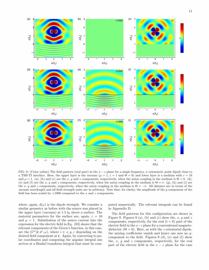
FIG. 9: (Color online) The field pattern (real part) in the x− z plane for a single frequency, x orientated, point dipole close toa TSB-TI interface. Here, the upper layer is the vacuum (µ = 1, ε = 1 and Θ = 0) and lower layer is a medium with ε = 16and µ = 1. (a), (b) and (c) are the x, y and z components, respectively, when the axion coupling in the medium is Θ = 0. (d),(e) and (f) are the x, y and z components, respectively, when the axion coupling in the medium is Θ = π. (g), (h) and (i) arethe x, y and z components, respectively, when the axion coupling in the medium is Θ = −π. All distance are in terms of thevacuum wavelength and all field strength units are in arbitrary. Note that, for clarity, the amplitude of the y component of thefield has been scaled by ×1000 compared to the x and z components.

where, again, d(ω) is the dipole strength. We consider asimilar geometry as before with the source was placed inthe upper layer (vacuum) at 1.5λ0 above a surface. Thematerial parameters for the surface are, again, ε = 16and µ = 1. Substitution of the source current into theexpression for the electric field in Eq. (83) shows that therelevant components of the Green’s function, in this case,are the Gix(r, r′, ω), where i ∈ x, y, z depending on thedesired field component at r. Again, by converting to po-lar coordinates and computing the angular integral onearrives at a Hankel transform integral that must be com-

puted numerically. The relevant integrals can be foundin Appendix D.

The field patterns for this configuration are shown inFigure 9. Figures 9 (a), (b) and (c) show the, x, y and zcomponents, respectively, for the real (t = 0) part of theelectric field in the x−z plane for a conventional magneto-dielectric (Θ = 0). Here, as with the z-orientated dipole,the mixing coefficients vanish and hence one sees no y-component to the field. Figures 9 (d), (e) and (f) showthe, x, y and z components, respectively, for the realpart of the electric field in the x − z plane for the case

12

of a TSB-TI with, Θ = π. One, again, sees the gener-ation of a non-zero y-component owing to the effects ofthe interface. Figures 9 (g), (h) and (i) show the, x, yand z components, respectively, for the real part of theelectric field in the x− z plane for the case of a TSB-TIwith, Θ = −π. As before we see the inversion of they-component compared to that in Figure 9 (e). Again,the discontinuity in Figures 9 (c), (f) and (i) is expectedsince this is the longitudinal component of the electricfield.

VIII. SUMMARY

We have constructed the Green’s function of a layeredTSB-TI and used it to study the field pattern of a singlefrequency point dipole close to the surface of a topolog-ical insulator. Reflection and transmission from a TSB-TI surface leads to mixing of TE and TM polarizationcomponents and hence a rotation in the overall polariza-tion of the incident light. This effect has the potentialto be the basis for a number of novel optical and quan-tum optical effects, for whose study the Green’s functionwill be useful. Owing to the ubiquitous nature of theGreen’s function in both classical and quantum electro-magnetism, it is hoped that the closed form expressionsfor this function will prove to be beneficial to a greatmany fields.

IX. ACKNOWLEDGEMENTS

This work was supported by the DFG (grants BU1803/3-1 and GRK 2079/1). SYB is grateful for supportby the Freiburg Institute for Advanced Studies.

Appendix A: Schwarz Reflection Principle

The Schwarz reflection principle states that

G∗(r, r′, ω) = G(r, r′,−ω∗). (A1)

One can show that the same principle holds for axionicmaterials. Given the Helmholtz equation in Eq. (8), thedefinition of the Green’s function reads

∇× 1

µ(r, ω)∇×G(r, r′, ω)

− iωc

α

π[∇Θ(r, ω)×G(r, r′, ω)]

− ω2

c2ε(r, ω)G(r, r′, ω) = δ(r− r′). (A2)

Setting ω → −ω∗ gives

∇× 1

µ(r,−ω∗)∇×G(r, r′,−ω∗)

+ iω∗

c

α

π[∇Θ(r,−ω∗)×G(r, r′,−ω∗)]

− (ω∗)2

c2ε(r,−ω∗)G(r, r′,−ω∗) = δ(r− r′). (A3)

As the permittivity, ε(r, ω), and permeability, µ(r, ω),via causality arguments, also obey the Schwarz reflectionprinciple and the axion coupling, Θ(r, ω), is real, we have

∇× 1

µ∗(r, ω)∇×G(r, r′,−ω∗)

+ iω∗

c

α

π[∇Θ(r, ω)×G(r, r′,−ω∗)]

− (ω∗)2

c2ε∗(r, ω)G(r, r′,−ω∗) = δ(r− r′). (A4)

By comparing Eq. (A4) with the complex conjugate ofEq. (A2), one can see that the Schwarz reflection princi-ple holds for axionic materials.

For purely imaginary frequencies one has

G∗(r, r′, iξ) = G(r, r′,− (iξ)∗) = G(r, r′, iξ), (A5)

where ξ is real. Hence at imaginary frequencies theGreen’s function is real. In addition one has,

kz =

√(iξ)2

c2− k2p = i

√ξ2

c2+ k2p = iκz, (A6)

where κz is real. Substituting this into the expressionfor the Green’s function in Appendix B, converting toangular coordinates, performing the angular integrationand noting that the resulting Hankel transform is realone can see that the components of the planar half spaceGreen’s function obey the Schwarz reflection principle.

Appendix B: Greens Function for a Planar HalfSpace

The half space Green’s function has a single interfaceat z = 0, hence d± = 0. Hence, the multiple reflection co-

efficients M ij = I. For a source point in the upper layer,the upper reflection and transmission coefficients vanish,R+ = T+ = 0, and the lower reflection and transmission

coefficients becomes that for a single interface, R− = R

and T− = T . Similarly, for a source point in the lowerlayer, the lower reflection and transmission coefficientsvanish, R− = T− = 0, and the upper reflection coeffi-

cient becomes that for a single interface, R+ = R and

T+ = T . Putting this together, expanding the dyads,and ignoring the extracted singularity, leads to expres-sions for the reflective, transmissive and free space partsof the Green’s function for a source and field point in anarbitrary layer.

13

The free space part of the Green’s function is propor-tional to I and is given by the well known expression

G0(r, r′, ω) = µ(ω)

[1

k2∇⊗∇ + I

]eikR

4πR, (B1)

which, on evaluating the derivatives, becomes

G0(r, r′, ω) = µ(ω)eikR

4πR

[(1 +

ikR− 1

k2R2

)I

+3− 3ikR− k2R2

k2R2

R⊗R

R2

], (B2)

with R = r− r′.The reflective part of the Green’s function can be writ-

ten as

G(r, r′) =

∫d2kp(2π)2

eikp·(rp−r′p)Rij(kp, kz, z, z′), (B3)

with

Rxx(kp, kz, z, z′) =

iµ(ω)

2kzeikz(|z|+|z

′|)

×

[k2yk2pRTE,TE −

k2xk2z

k2pk2RTM,TM

+sgn (z′)kzk2pk

(kxkyRTE,TM − kxkyRTM,TE)

],

(B4)

Ryy(kp, kz, z, z′) =

iµ(ω)

2kzeikz(|z|+|z

′|)

×

[k2xk2pRTE,TE −

k2yk2z

k2pk2RTM,TM

−sgn (z′)kzk2pk

(kxkyRTE,TM − kxkyRTM,TE)

],

(B5)

Rxy(kp, kz, z, z′) =

iµ(ω)

2kzeikz(|z|+|z

′|)

×[−kxky

k2pRTE,TE −

kxkyk2z

k2pk2RTM,TM

+sgn (z′)kzk2pk

(k2yRTE,TM + k2xRTM,TE

)], (B6)

Ryx(kp, kz, z, z′) =

iµ(ω)

2kzeikz(|z|+|z

′|)

×[−kxky

k2pRTE,TE −

kxkyk2z

k2pk2RTM,TM

−sgn (z′)kzk2pk

(k2xRTE,TM + k2yRTM,TE

)], (B7)

Rxz(kp, kz, z, z′) =

iµ(ω)

2kzeikz(|z|+|z

′|)

×[−sgn (z′)

kxkzk2

RTM,TM +kykRTE,TM

], (B8)

Rzx(kp, kz, z, z′) =

iµ(ω)

2kzeikz(|z|+|z

′|)

×[sgn (z′)

kxkzk2

RTM,TM +kykRTM,TE

], (B9)

Ryz(kp, kz, z, z′) =

iµ(ω)

2kzeikz(|z|+|z

′|)

×[−sgn (z′)

kykzk2

RTM,TM −kxkRTE,TM

], (B10)

Rzy(kp, kz, z, z′) =

iµ(ω)

2kzeikz(|z|+|z

′|)

×[sgn (z′)

kykzk2

RTM,TM −kxkRTM,TE

], (B11)

Rzz(kp, kz, z, z′) =

iµ(ω)

2kzeikz(|z|+|z

′|)

[k2pk2RTM,TM

],

(B12)where µ(ω) is the permeability in the layer.

Similarly, the transmissive part of the Green’s functioncan be written as

G(r, r′) =

∫d2kp(2π)2

eikp·(rp−r′p)T ij(kp, kz, z, z′), (B13)

with

T xx(kp, kz, z, z′) =

iµ′(ω)

2kz′eikz|z|+ikz′ |z

′|

×

[k2yk2pTTE,TE +

k2xkzkz′

k2pkk′ TTM,TM

+sgn (z′)1

k2p

(kxky

kz′

k′TTE,TM + kxky

kzkTTM,TE

)],

(B14)

T yy(kp, kz, z, z′) =

iµ′(ω)

2kz′eikz|z|+ikz′ |z

′|

×

[k2xk2pTTE,TE +

k2ykzkz′

k2pkk′ TTM,TM

−sgn (z′)1

k2p

(kxky

kz′

k′TTE,TM + kxky

kzkTTM,TE

)],

(B15)

14

T xy(kp, kz, z, z′) =

iµ′(ω)

2kz′eikz|z|+ikz′ |z

′|

×[−kxky

k2pTTE,TE +

kxkykzkz′

k2pkk′ TTM,TM

+sgn (z′)1

k2p

(k2ykz′

k′TTE,TM − k2x

kzkTTM,TE

)],

(B16)

T yx(kp, kz, z, z′) =

iµ′(ω)

2kz′eikz|z|+ikz′ |z

′|

×[−kxky

k2pTTE,TE +

kxkykzkz′

k2pkk′ TTM,TM

−sgn (z′)1

k2p

(k2xkz′

k′TTE,TM − k2y

kzkTTM,TE

)],

(B17)

T xz(kp, kz, z, z′) =

iµ′(ω)

2kz′eikz|z|+ikz′ |z

′|

×[sgn (z′)

kxkzkk′

TTM,TM +kyk′TTE,TM

], (B18)

T zx(kp, kz, z, z′) =

iµ′(ω)

2kz′eikz|z|+ikz′ |z

′|

×[sgn (z′)

kxkz′

kk′TTM,TM +

kykTTM,TE

], (B19)

T yz(kp, kz, z, z′) =

iµ′(ω)

2kz′eikz|z|+ikz′ |z

′|

×[sgn (z′)

kykzkk′

TTM,TM −kxk′TTE,TM

], (B20)

T zy(kp, kz, z, z′) =

iµ′(ω)

2kz′eikz|z|+ikz′ |z

′|

×[sgn (z′)

kykz′

kk′TTM,TM −

kxkTTM,TE

], (B21)

T zz(kp, kz, z, z′) =

iµ′(ω)

2kz′eikz|z|+ikz′ |z

′|

[k2pkk′

TTM,TM

],

(B22)where µ′(ω) is the permeability in the source layer.Note that if the cross-reflection, RTE,TM and RTM,TE

and cross-transmission, TTM,TE and TTM,TE , coefficientsvanish one recovers the Green’s function for a conven-tional magneto-dielectric [22].

Appendix C: Green’s Function Components for anz-Orientated Dipole

The field from a z-orientated dipole close to a TSB-TIcan be found from the planar half space Green’s func-tion in Appendix B. The relevant components can be

simplified by converting to polar coordinate, after whichthe angular integral can be computed analytically. Theresulting Hankel transforms, which must be evaluatednumerically, are

Rxz(r, r′) =1

4π

∫dkp e

ikz(|z|+|z′|)

× J1 (kpRp)k2pk2RTM,TM , (C1)

Ryz(r, r′) =1

4π

∫dkp e

ikz(|z|+|z′|)

× J1 (kpRp)k2pkkz

RTE,TM , (C2)

Rzz(r, r′) =i

4π

∫dkp e

ikz(|z|+|z′|)

× J0 (kpRp)k3pk2kz

RTM,TM , (C3)

for the reflective part and

T xz(r, r′) = − 1

4π

∫dkp e

ikz|z|+ikz′ |z′|

× J1 (kpRp)k2pkz

kk′kz′TTM,TM , (C4)

T yz(r, r′) =1

4π

∫dkp e

ikz|z|+ikz′ |z′|

× J1 (kpRp)k2pk′kz′

TTE,TM , (C5)

T zz(r, r′) =i

4π

∫dkp e

ikz|z|+ikz′ |z′|

× J0 (kpRp)k3p

kk′kz′TTM,TM , (C6)

for the transmissive part, where Rp = rp − r′p.

Appendix D: Green’s Function Components for anx-Orientated Dipole

The field from a x-orientated dipole close to a TSB-TIcan, again, be found from the planar half space Green’sfunction in Appendix B. Converting to polar coordinateand evaluating the angular integral leads to

Rxx(r, r′) =i

8π

∫dkp e

ikz(|z|+|z′|)

×

[J0 (kpRp) + 2J2 (kpRp)]kpkzRTE,TE

− [J0 (kpRp)− 2J2 (kpRp)]kpkzk2

RTM,TM

, (D1)

15

Ryx(r, r′) = − i

8π

∫dkp e

ikz(|z|+|z′|)

×

[J0 (kpRp)− 2J2 (kpRp)]kpkRTE,TM

+ [J0 (kpRp) + 2J2 (kpRp)]kpkRTM,TE

, (D2)

Rzx(r, r′) = − 1

4π

∫dkp e

ikz(|z|+|z′|)

×

J1 (kpRp)

k2pk2RTM,TM

, (D3)

for the reflective part and

T xx(r, r′) =i

8π

∫dkp e

ikz|z|+ikz′ |z′|

×

[J0 (kpRp) + 2J2 (kpRp)]kpkz′

TTE,TE

+ [J0 (kpRp)− 2J2 (kpRp)]kpkzkk′

TTM,TM

, (D4)

T yx(r, r′) = − i

8π

∫dkp e

ikz|z|+ikz′ |z′|

×

[J0 (kpRp)− 2J2 (kpRp)]kpk′TTE,TM

− [J0 (kpRp) + 2J2 (kpRp)]kpkzkkz′

TTM,TE

, (D5)

T zx(r, r′) = − 1

4π

∫dkp e

ikz|z|+ikz′ |z′|

×

J1 (kpRp)

k2pkk′

TTM,TM

, (D6)

for the transmissive part.

[1] M. Z. Hasan and C. L. Kane, Rev. Mod. Phys. 82, 3045(2010).

[2] X.-L. Qi and S.-C. Zhang, Rev. Mod. Phys. 83, 1057(2011).

[3] B. A. Bernevig, T. L. Hughes and S.-C. Zhang, Science314, 1757 (2006).

[4] Markus Konig, S. Wiedmann, Christoph Brune, A. Roth,H. Buhmann, L. W. Molenkamp, X.-L. Qi and S.-C.Zhang, Science 318, 766 (2007).

[5] L. Fu and C. L. Kane, Phys. Rev. B 76, 045302 (2007).[6] D. Hsieh, D. Qian, L. Wray, Y. Xia, Y. S. Hor, R. J. Cava

and M. Z. Hasan, Nature 452, 970 (2008).[7] H. Zhang, C.-X. Liu, X.-L. Qi, X. Dai, Z. Fang and S.-C.

Zhang, Nat. Phys. 5, 438 (2009).[8] C.-X. Liu, X.-L. Qi, H. Zhang, X. Dai, Z. Fang and S.-C.

Zhang, Phys. Rev. B 82, 045122 (2010).[9] C. L. Kane and E. J. Mele, Phys. Rev. Lett. 95, 146802

(2005).[10] B. A. Bernevig and S.-C. Zhang, Phys. Rev. Lett. 96,

106802 (2006).[11] X.-L. Qi, R. Li, J. Zang and S.-C. Zhang, Science 323,

1184 (2009).[12] X.-L. Qi, T. L. Hughes and S.-C. Zhang, Phys. Rev. B

78, 195424 (2008).[13] M.-C. Chang and M.-F. Yang, Phys. Rev. B 80, 113304

(2009).[14] A. G. Grushin and A. Cortijo, Phys. Rev. Lett. 106,

020403 (2011).[15] A. G. Grushin, P. Rodriguez-Lopez and A. Cortijo, Phys.

Rev. B 84, 045119 (2011).[16] F. Wilczek, Phys. Rev. Lett 58, 1799 (1987).[17] Y. N. Obukhov and F. W. Hehl, Phys. Lett. A 341, 357

(2005).[18] Y. L. Chen, J.-H. Chu, J. G. Analytis, Z. K. Liu, K.

Igarashi, H.-H. Kuo, X. L. Qi, S. K. Mo, R. G. Moore,D. H. Lu, M. Hashimoto, T. Sasagawa, S. C. Zhang, I.R. Fisher, Z. Hussain and Z. X. Shen, Science 329, 659(2010).

[19] J. Maciejko, X.-L. Qi, H. D. Drew and S.-C. Zhang, Phys.Rev. Lett. 105, 166803 (2010).

[20] W. C. Chew, Waves and Fields in Inhomogeneous Media(IEEE Press, 1995).

[21] J. D. Jackson, Classical Electrodynamics, 3rd Ed. (JohnWiley & Sons, 1998).

[22] H. T. Dung, L. Knoll, and D.-G. Welsch, Phys. Rev. A57, 3931 (1997).

[23] S. Scheel and S.Y. Buhmann, Acta Phys. Slov. 58, 675(2008).

[24] S. Y. Buhmann, Dispersion Forces I (Springer, 2012).[25] S. Y. Buhmann, D. T. Butcher and S. Scheel, New J.

Phys. 14, 083034 (2012).[26] T. Gruner and D.-G. Welsch, Phys. Rev. A 54, 1661

(1996).[27] J. A. Crosse and S. Scheel, Phys. Rev. A 81, 033815

(2010).[28] J. A. Crosse and S. Scheel, Phys. Rev. A 83, 023815

(2011).[29] S. Y. Buhmann, L. Knoll, D.-G. Welsch and H. T. Dung,

Phys. Rev. A 70, 052117 (2004).[30] S. Y. Buhmann and S. Scheel, Phys. Rev. Lett 100,

253201 (2008).[31] J. A. Crosse, S. A. Ellingsen, K. Clements, S. Y. Buh-

mann and Stefan Scheel, Phys. Rev. A 82, 010901(R)(2010).

[32] R. Fermani, S. Scheel and P. L. Knight, Phys. Rev. A73, 032902 (2006).

[33] P. K. Rekdal, S. Scheel, P. L. Knight and E. A. Hinds,Phys. Rev. A 70, 013811 (2004).

16

[34] S. Y. Buhmann, M. R. Tarbutt, S. Scheel and E. A.Hinds, Phys. Rev. A 78, 052901 (2008).

[35] S. A. Ellingsen, S. Y. Buhmann and S. Scheel, Phys. Rev.A 79, 052903 (2008).

[36] O. Madelung, U. Rossler, M. Schulz; SpringerMaterials;sm lbs 978-3-540-31360-1 945 (Springer-Verlag GmbH,Heidelberg, 1998).