THE EFFECTS OF

THE TAXATION OF FOREIGN DIRECT INVESTMENT: AN EMPIRICAL ASSESSMENT

Candidate Number: 78953

2

Contents I. Introduction _______________________________________________________3

II. Foreign Direct Investment: Definition and Developments ______________________3

1. Definition ______________________________________________________________ 3

2. FDI flows since 1979 _____________________________________________________ 4

III. Determinants of FDI flows - theory _____________________________________6

1. Models ________________________________________________________________ 6

2. Parameters _____________________________________________________________ 7

IV. Determinants of FDI flows - evidence ________________________________ ____9

1. The data _______________________________________________________________ 9

2. The models and the estimation procedure ___________________________________ 13 a) Model I________________________________________________________________________ 13 b) Model II _______________________________________________________________________ 14 c) The estimation procedure __________________________________________________________ 14

3. Results _______________________________________________________________ 16 a) Model I________________________________________________________________________ 16 b) Model II _______________________________________________________________________ 18

4. Limitations of the analysis ________________________________________________ 19

5. Implications for the theories of FDI determination ____________________________ 20

6. Comparison with selected literature ________________________________________ 21

V. Conclusion________________________________ _______________________22 References ________________________________________________________________________ 23 Appendix I - Technical Notes __________________________________________________________ 24

I. Introduction This essay analyses the effect of taxes on foreign direct investment (FDI). The second part examines

the different aspects of FDI, namely the definition of FDI and the extent of FDI flows since 1979.

Theoretical explanations for the existence of such flows are considered in part III. Those are industrial

organisation theories, the cost-of-capital approach, corporate investment theory, and portfolio theory.

The fourth part uses two data panels to examine the determinants of FDI flows, and evaluates the

different theories of FDI determination in the light of the evidence obtained. While the first panel

contains FDI flows into 7 industrialised countries, the second panel features FDI inflows into the UK

economy from 9 OECD countries. The period under consideration is 1979-1994. The final part of the

essay summarises and concludes the discussion.

II. Foreign Direct Investment: Definition and Developments

1. Definition As the academic literature does not always agree about the definition of FDI, it seems appropriate to

turn to the definition of an official organisation. According to OECD (1996), ‘foreign direct investment

reflects the objective of obtaining a lasting interest by a resident entity in one country (‘direct investor’)

in an entity resident in an economy other than that of the investor (‘direct investment enterprise’). The

lasting interest implies the existence of a long-term relationship between the direct investor and the

enterprise and a significant degree of influence on the management of the enterprise.’ To implement

this statement, the OECD recommends that ‘a direct investment enterprise be defined as an [...]

enterprise in which a foreign investor owns 10 percent or more of the ordinary shares or voting power

of an [...] enterprise’. The important aspects of this definition are that FDI involves a ‘lasting interest’,

a ‘long-term relationship’, and a ‘significant degree of influence’, although the latter part of the

definition has increasingly become less important in recent years (Lipsey, 1999). These aspects will

become important once the essay turns to theoretical models of FDI determination.

Looking at total international investment flows, the IMF1 reports two categories other than

FDI. First, portfolio investment, which includes equity securities, debt securities in form of bonds,

money market instruments, and financial derivatives, such as options, all excluding any of these

included in direct investment or reserve assets. Second, ‘other investment’, such as trade credit, loans,

financial leases, currency, and deposits, mostly short-term assets.

1 E.g. IMF (1996).

4

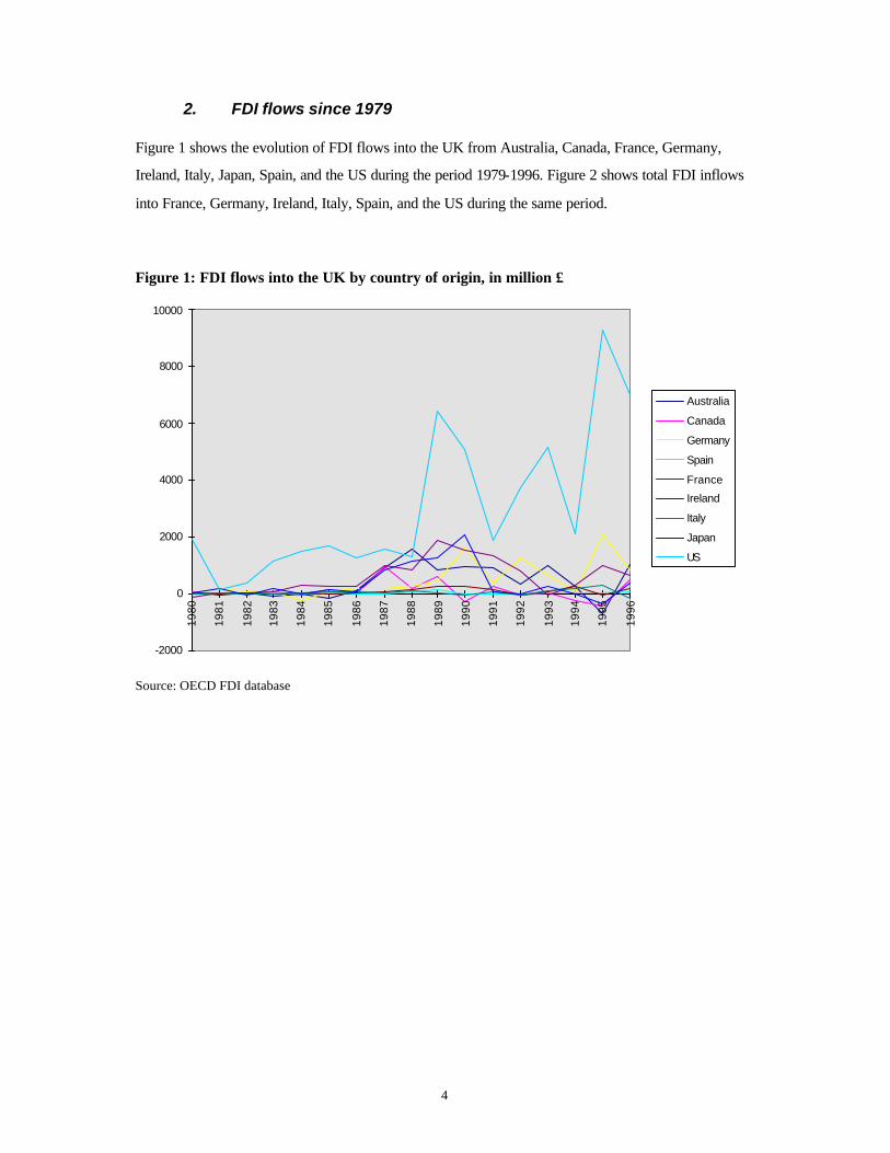
2. FDI flows since 1979 Figure 1 shows the evolution of FDI flows into the UK from Australia, Canada, France, Germany,

Ireland, Italy, Japan, Spain, and the US during the period 1979-1996. Figure 2 shows total FDI inflows

into France, Germany, Ireland, Italy, Spain, and the US during the same period.

Figure 1: FDI flows into the UK by country of origin, in million £

-2000

0

2000

4000

6000

8000

10000

1980

1981

1982

1983

1984

1985

1986

1987

1988

1989

1990

1991

1992

1993

1994

1995

1996

Australia

Canada

Germany

Spain

France

Ireland

Italy

Japan

US

Source: OECD FDI database

5

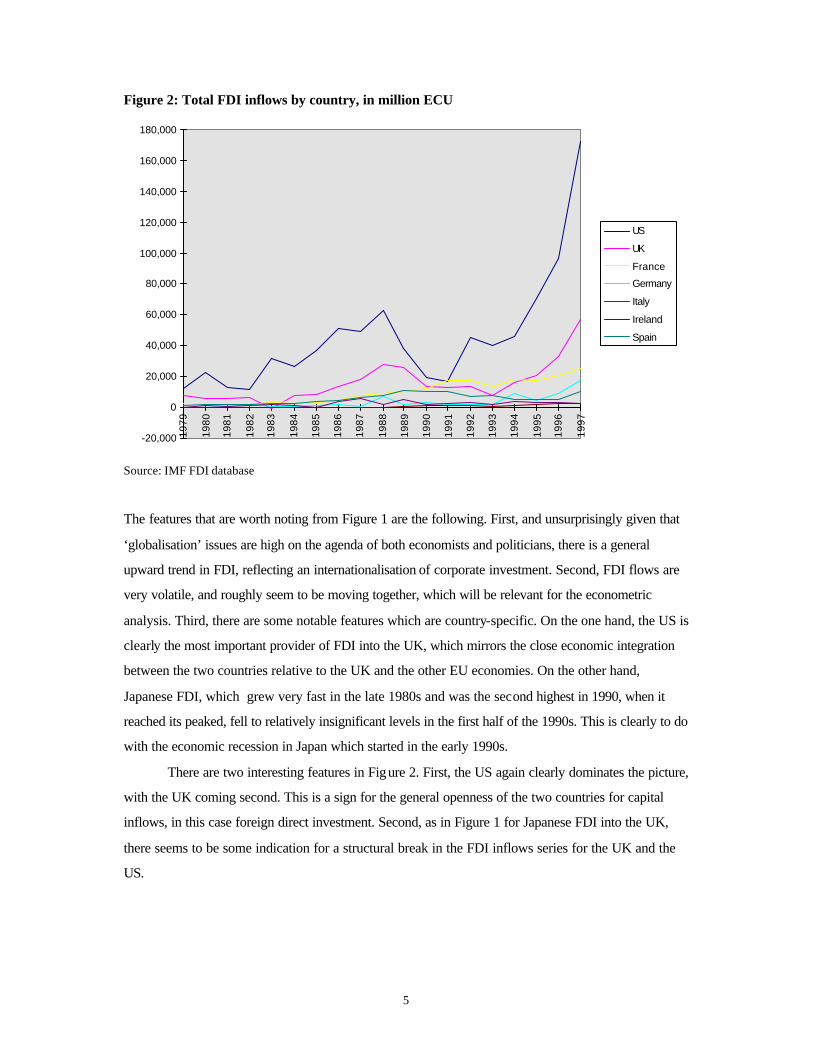
Figure 2: Total FDI inflows by country, in million ECU

-20,000

0

20,000

40,000

60,000

80,000

100,000

120,000

140,000

160,000

180,000

1979

1980

1981

1982

1983

1984

1985

1986

1987

1988

1989

1990

1991

1992

1993

1994

1995

1996

1997

US

UK

France

Germany

Italy

Ireland

Spain

Source: IMF FDI database The features that are worth noting from Figure 1 are the following. First, and unsurprisingly given that

‘globalisation’ issues are high on the agenda of both economists and politicians, there is a general

upward trend in FDI, reflecting an internationalisation of corporate investment. Second, FDI flows are

very volatile, and roughly seem to be moving together, which will be relevant for the econometric

analysis. Third, there are some notable features which are country-specific. On the one hand, the US is

clearly the most important provider of FDI into the UK, which mirrors the close economic integration

between the two countries relative to the UK and the other EU economies. On the other hand,

Japanese FDI, which grew very fast in the late 1980s and was the second highest in 1990, when it

reached its peaked, fell to relatively insignificant levels in the first half of the 1990s. This is clearly to do

with the economic recession in Japan which started in the early 1990s.

There are two interesting features in Figure 2. First, the US again clearly dominates the picture,

with the UK coming second. This is a sign for the general openness of the two countries for capital

inflows, in this case foreign direct investment. Second, as in Figure 1 for Japanese FDI into the UK,

there seems to be some indication for a structural break in the FDI inflows series for the UK and the

US.

6

III. Determinants of FDI flows - theory

1. Models The literature on the causes of FDI is very large. In this section, its main strands are described.

Industrial organisation. This approach postulates that firm-specific characteristics (e.g. product

technology, management skills, economies of scale) are the major determinant of FDI, as they

confer certain advantages on foreign subsidiaries. One of the ma in assumptions of this model is that

the investing firm cannot reap the benefits from these advantages simply by a licensing process. For

example, an invention or a production process is very difficult to value, and in the presence of

asymmetric information it is even more difficult to get two companies to agree on a price. The

benefits from a patent can therefore be reaped more easily by assuming the (partial) control of a

company that is interested in using this patent, i.e. by internalising the operations of the foreign firm.

Cost of capital (Graham and Krugman, 1995). A foreign firm might be willing to invest in a

domestic firm because it applies a lower discount rate to expected cash flows. This approach

focuses on firm-specific aspects.

Corporate inv estment theory. Here, locational aspects play the most important role in

determining FDI. These include the importance of the size of the host market, factor prices,

protection afforded to investing firms by tariffs and/or other measures.

Portfolio theory (Brainard and Tobin, 1992). FDI is modelled as part of a portfolio choice of the

investor. This theory is basically introducing FDI into the capital-asset-pricing model (CAPM). FDI

leads to a diversification of the portfolio of the foreign company, which reduces overall risk.

The first three approaches all imply directly that the foreign firm engages in FDI because of its pursuit

of the highest return to its resources. This will also be true for portfolio-theory explanations, although

here the diversification motive is added. Therefore, these four explanations of the determinants of FDI

are not exclusive, on the contrary. As Dunning (1993) points out, locational aspects and firm-specific

aspects interact with the advantages of internalisation.

7

2. Parameters Given the different theories at hand, one should be able to single out different factors which have got

the potential to affect FDI. These are the following.

The exchange rate . Graham and Krugman (1995) point out that, although a depreciation of the

home currency makes domestic firms more attractive for foreign firms because of higher net

expected returns, those higher net expected returns are exactly the same for other domestic firms.

Thus, FDI should not change as a result.

On the other hand, a falling home currency shifts the domestic economy more towards the

tradable sector. As FDI is higher in the tradable sector, this mechanism leads to a link between

depreciation and FDI, although only indirectly. Furthermore, Froot and Stein (1991) show that a

depreciation should lead to higher FDI because of the wealth effect on foreign firms. A depreciation

raises the book value of foreign firms relative to domestic firms. In an imperfect capital market with

credit-constrained firms, a rising book value leads to greater buying power and therefore to

potentially higher FDI. Finally, foreign investors might not act fully rationally when they are

confronted with a depreciation of the home currency. They might only compare home assets which

appear cheap in comparison to assets abroad, while they neglect that economic returns might not be

equivalent. Thus, there seem to be enough theoretical explanations for the importance of exchange

rates on FDI.

Interest rates have an impact on the cost of capital, and therefore the discount rate. According to

the cost-of-capital view, interest rate differentials between countries consequently have got the

potential to influence FDI flows.

Tax rates on corporate income affect the extent to which the investing firm can appropriate the

profits it has earned from its foreign direct investment. One has to distinguish between three

different tax rates2:

(i) the statutory tax rate: generally the most visible aspect of the tax system. It might therefore

play a role through some ‘signalling function’, although in practice in many cases it is not the

tax rate that actually applies to a provider of FDI.

(ii) The effective marginal tax rate (EMTR). The EMTR applies to a marginal investment project.

This is an investment project which makes the foreign firm just indifferent between investing and

not investing. In other words, such a project just earns the required rate of return.

2 The following paragraph draws on the analysis in Chennels and Griffith (1997). Technical details in Appendix I

8

The effective marginal tax rate measures the tax wedge as a proportion of the investing firm’s

post-tax return, where the tax wedge is the difference between the pre-tax rate of return earned

by the company on that marginal investment project and the post-tax rate of return earned by the

investor.

(iii) The effective average tax rate (EATR). The EATR, on the other hand, applies to an

investment project that earns some economic rent, i.e. that earns more than the required rate of

return. The EATR is the difference in the present value of the investment project in the absence

and in the presence of tax, as a proportion of the present value of the project in the absence of

tax. In contrast to the EMTR, the EATR is the relevant measure for comparing large investment

projects.

This means: EMTRs look at the last penny flowing into an investment project, while EATRs look at

all the funds flowing into a project. In the case of FDI, this means that these effective tax rates

model two different decisions (Devereux and Griffith, 1998). The EATR models the discrete choice

of a foreign firm whether it should invest in a new project in the home economy. When making this

decision, the relevant criterion for the investor is the aggregate profitability of the project. In

contrast to that, the EMTR determines how much money should flow into an FDI project, given that

the locational decision has already been taken. It is an empirical matter to determine which tax rate

plays the more important role in practice.

According to Chennels and Griffith (1997), effective tax rates summarise the impact of the tax

system on the required rate of return, taking into account both differences in tax rates and

differences in the tax base. They ‘reflect differences in capital allowances, relief for inflationary

gains on holdings of inventories, the structure of the tax system, whether or not capital gains are

indexed for inflation, withholding taxes and other aspects of international tax treaties.’

Business cycle effects can play a role in determining FDI as well. As a matter of economic

theory, it is not clear why business cycles in the home economy should make assets more attractive.

The long-term growth rate of the economy should be more important in this respect. However, the

growth rate of the foreign economy can be significant theoretically if one deals with imperfect

capital markets. Similarly to the exchange rate effects, cash-constrained investors might use their

increased cash-flow to finance the acquisition of foreign assets.

9

IV. Determinants of FDI flows - evidence

1. The data FDI data comes from the IMF International Financial Statistics. It is important to realis e that these data

are not without problems. Comparison with OECD data3 show discrepancies between the two sources.

Furthermore, Eurostat4 repeatedly report differences between ‘mirror flows’, i.e. a discrepancy

between what the foreign country claims to ha ve invested in the home country and what the home

country claims to have received from the foreign country. This often arises because of differences in

the definition of FDI between countries. However, these problems do not seem to be substantial

enough to invalidate the analysis, as the tendencies reported coincide.

The exchange rate is taken from two sources. Nominal bilateral exchange rates between the

pound and the various other currencies are from Datastream, with the real exchange rate calculated

using the implicit GDP deflator. Effective real exchange rates are from the OECD National Accounts

database5. Interest rates are from the IMF Financial Statistics Yearbook. The interest rate chosen was

the lending rate, in order to model the cost of capital. Nominal GDP figures are from the OECD

National Accounts database, and transformed into real terms using the implicit GDP deflator. These

were used to calculate growth rates which capture business cycle effects.

The various tax rates used here are taken from Chennells and Griffith (1997). In order to obtain

aggregate rates for national economies, they use the following methodology. Effective rates are

calculated by taking averages across finance and assets. Weights are as follows: 28% for buildings,

50% for plant and machinery, 22% for inventories; 55% for retained earnings, 10% for new equity,

35% for debt. The inflation rate and the real interest rate are assumed to be constant at 3.5% and 10%,

respectively. The personal tax rate of the marginal investor is assumed to be zero. The series on

effective tax rates restrict the analysis from going beyond 1994, as EATR and EMTR are only

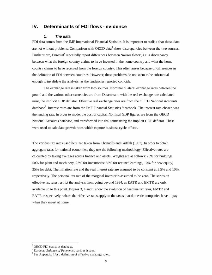
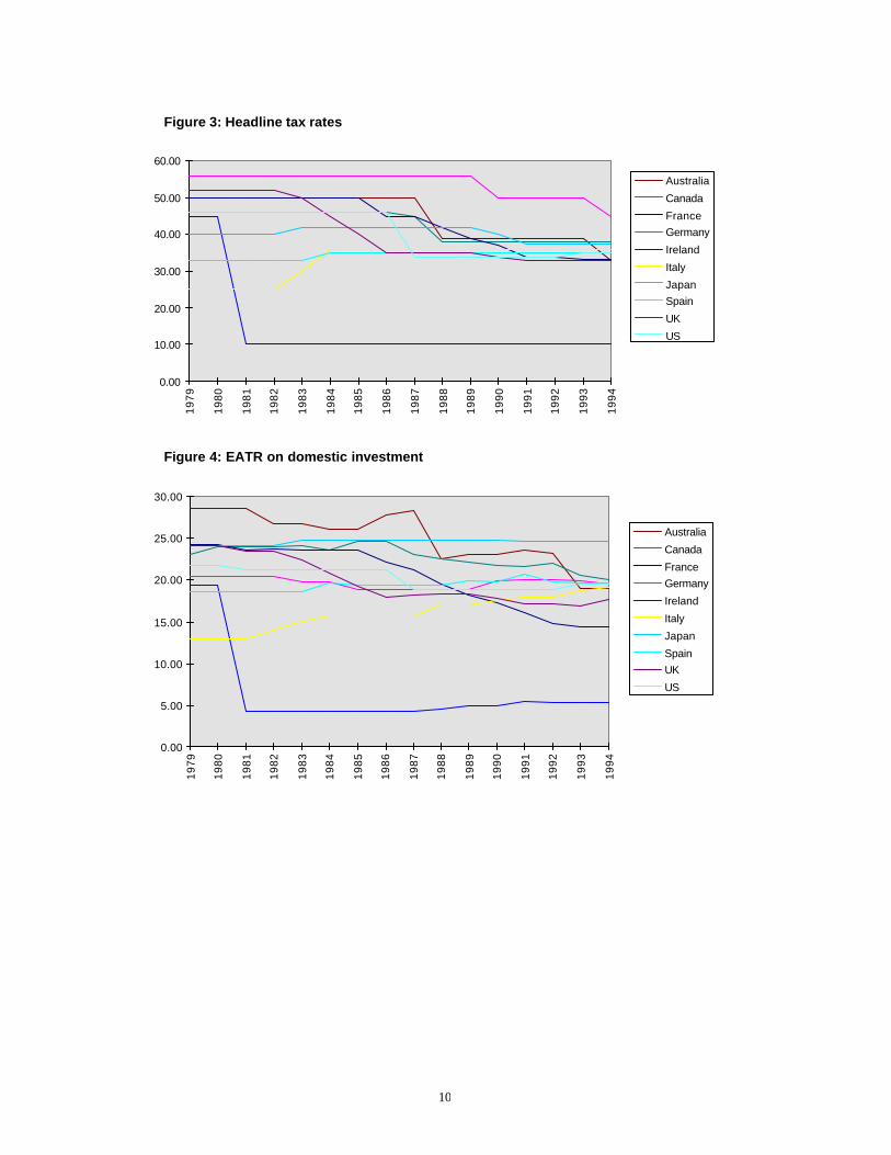
available up to this point. Figures 3, 4 and 5 show the evolution of headline tax rates, EMTR and

EATR, respectively, where the effective rates apply to the taxes that domestic companies have to pay

when they invest at home.

3 OECD FDI statistics database. 4 Eurostat, Balance of Payments , various issues. 5 See Appendix I for a definition of effective exchange rates.

10

Figure 3: Headline tax rates

0.00

10.00

20.00

30.00

40.00

50.00

60.00

1979

1980

1981

1982

1983

1984

1985

1986

1987

1988

1989

1990

1991

1992

1993

1994

Australia

Canada

FranceGermany

Ireland

Italy

JapanSpain

UK

US

Figure 4: EATR on domestic investment

0.00

5.00

10.00

15.00

20.00

25.00

30.00

1979

1980

1981

1982

1983

1984

1985

1986

1987

1988

1989

1990

1991

1992

1993

1994

Australia

Canada

FranceGermany

Ireland

Italy

Japan

SpainUK

US

11

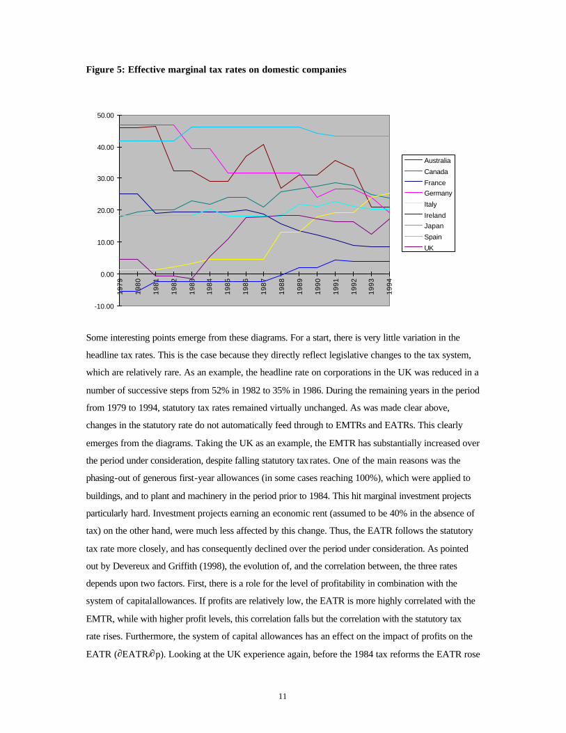
Figure 5: Effective marginal tax rates on domestic companies

-10.00

0.00

10.00

20.00

30.00

40.00

50.0019

79

1980

1981

1982

1983

1984

1985

1986

1987

1988

1989

1990

1991

1992

1993

1994

Australia

Canada

FranceGermany

Italy

IrelandJapan

Spain

UK

Some interesting points emerge from these diagrams. For a start, there is very little variation in the

headline tax rates. This is the case because they directly reflect legislative changes to the tax system,

which are relatively rare. As an example, the headline rate on corporations in the UK was reduced in a

number of successive steps from 52% in 1982 to 35% in 1986. During the remaining years in the period

from 1979 to 1994, statutory tax rates remained virtually unchanged. As was made clear above,

changes in the statutory rate do not automatically feed through to EMTRs and EATRs. This clearly

emerges from the diagrams. Taking the UK as an example, the EMTR has substantially increased over

the period under consideration, despite falling statutory tax rates. One of the main reasons was the

phasing-out of generous first-year allowances (in some cases reaching 100%), which were applied to

buildings, and to plant and machinery in the period prior to 1984. This hit marginal investment projects

particularly hard. Investment projects earning an economic rent (assumed to be 40% in the absence of

tax) on the other hand, were much less affected by this change. Thus, the EATR follows the statutory

tax rate more closely, and has consequently declined over the period under consideration. As pointed

out by Devereux and Griffith (1998), the evolution of, and the correlation between, the three rates

depends upon two factors. First, there is a role for the level of profitability in combination with the

system of capital allowances. If profits are relatively low, the EATR is more highly correlated with the

EMTR, while with higher profit levels, this correlation falls but the correlation with the statutory tax

rate rises. Furthermore, the system of capital allowances has an effect on the impact of profits on the

EATR (∂EATR/∂p). Looking at the UK experience again, before the 1984 tax reforms the EATR rose

12

with profitability (i.e. ∂EATR/∂p > 0), while afterwards the opposite was the case (i.e. ∂EATR/∂p <

0)6. The second important factor is the way personal and corporate taxation are integrated.

Corporate income can be subject to two levels of taxation, corporate income tax and personal

income tax. There are broadly four ways of dealing with this problem. Under a classical system, as

operated in the US, corporate income is indeed taxed at those two levels. A split-rate system (e.g.

Australia until 1987, Japan until 1990) applies two different tax rates, depending on whether earnings

are retained or distributed. In this case, distributed earnings are taxed at a lower rate than retained

earnings, in order to compensate for personal income taxes that have to be paid. Under an imputation

system (in operation in Canada, France, Ireland, Italy, and the UK) personal income taxes are reduced

according to corporate income taxes paid on distributed profits. Finally, countries such as Japan operate

a partial shareholder relief system. These different features of the tax system have to be taken into

account when calculating effective tax rates.

A second set of tax rates emerges from the consideration of cross-border investments. These are the

tax rates that apply to investment from a foreign company into the domestic economy. Those rates are

depicted in figure 6 and figure 7.

Figure 6: EMTR on FDI in the domestic economy

0.00

10.00

20.00

30.00

40.00

50.00

60.00

70.00

80.00

90.00

1979

1980

1981

1982

1983

1984

1985

1986

1987

1988

1989

1990

1991

1992

1993

1994

AustraliaCanada

France

Germany

IrelandItaly

Japan

Spain

UKUS

6 As this essay is concerned with the years 1979-1994 only, developments outside this period, such as the 1997 tax reforms, are not dealt with here.

13

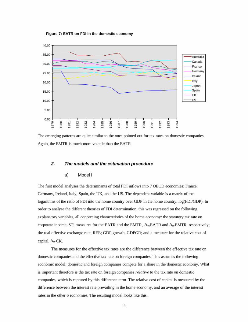
Figure 7: EATR on FDI in the domestic economy

0.00

5.00

10.00

15.00

20.00

25.00

30.00

35.00

40.00

1979

1980

1981

1982

1983

1984

1985

1986

1987

1988

1989

1990

1991

1992

1993

1994

Australia

Canada

FranceGermany

Ireland

Italy

JapanSpain

UK

US

The emerging patterns are quite similar to the ones pointed out for tax rates on domestic companies.

Again, the EMTR is much more volatile than the EATR.

2. The models and the estimation procedure

a) Model I The first model analyses the determinants of total FDI inflows into 7 OECD economies: France,

Germany, Ireland, Italy, Spain, the UK, and the US. The dependent variable is a matrix of the

logarithms of the ratio of FDI into the home country over GDP in the home country, log(FDI/GDP). In

order to analyse the different theories of FDI determination, this was regressed on the following

explanatory variables, all concerning characteristics of the home economy: the statutory tax rate on

corporate income, ST; measures for the EATR and the EMTR, ∆WEATR and ∆WEMTR, respectively;

the real effective exchange rate, REE; GDP growth, GDPGR; and a measure for the relative cost of

capital, ∆WCK.

The measures for the effective tax rates are the difference between the effective tax rate on

domestic companies and the effective tax rate on foreign companies. This assumes the following

economic model: domestic and foreign companies compete for a share in the domestic economy. What

is important therefore is the tax rate on foreign companies relative to the tax rate on domestic

companies, which is captured by this difference term. The relative cost of capital is measured by the

difference between the interest rate prevailing in the home economy, and an average of the interest

rates in the other 6 economies. The resulting model looks like this:

14

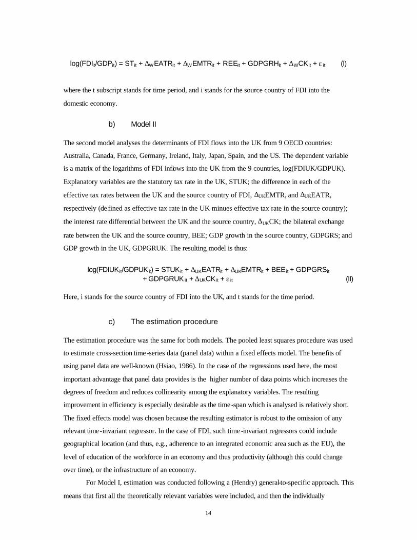
log(FDIit/GDPit) = STit + ∆WEATRit + ∆WEMTRit + REEit + GDPGRHit + ∆WCK it + ε it (I)

where the t subscript stands for time period, and i stands for the source country of FDI into the

domestic economy.

b) Model II The second model analyses the determinants of FDI flows into the UK from 9 OECD countries:

Australia, Canada, France, Germany, Ireland, Italy, Japan, Spain, and the US. The dependent variable

is a matrix of the logarithms of FDI inflows into the UK from the 9 countries, log(FDIUK/GDPUK).

Explanatory variables are the statutory tax rate in the UK, STUK; the difference in each of the

effective tax rates between the UK and the source country of FDI, ∆UKEMTR, and ∆UKEATR,

respectively (de fined as effective tax rate in the UK minues effective tax rate in the source country);

the interest rate differential between the UK and the source country, ∆UKCK; the bilateral exchange

rate between the UK and the source country, BEE; GDP growth in the source country, GDPGRS; and

GDP growth in the UK, GDPGRUK. The resulting model is thus:

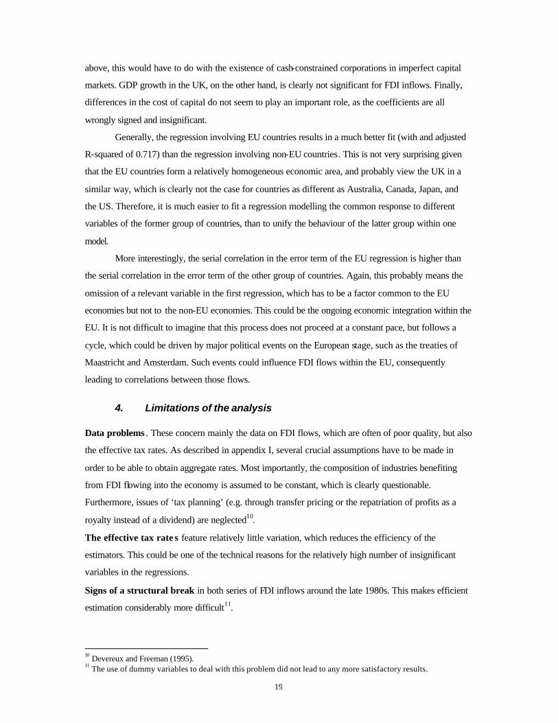
log(FDIUKit/GDPUK it) = STUKit + ∆UKEATRit + ∆UKEMTRit + BEE it + GDPGRSit

+ GDPGRUK it + ∆UKCK it + ε it (II) Here, i stands for the source country of FDI into the UK, and t stands for the time period.

c) The estimation procedure The estimation procedure was the same for both models. The pooled least squares procedure was used

to estimate cross-section time-series data (panel data) within a fixed effects model. The benefits of

using panel data are well-known (Hsiao, 1986). In the case of the regressions used here, the most

important advantage that panel data provides is the higher number of data points which increases the

degrees of freedom and reduces collinearity among the explanatory variables. The resulting

improvement in efficiency is especially desirable as the time-span which is analysed is relatively short.

The fixed effects model was chosen because the resulting estimator is robust to the omission of any

relevant time-invariant regressor. In the case of FDI, such time -invariant regressors could include

geographical location (and thus, e.g., adherence to an integrated economic area such as the EU), the

level of education of the workforce in an economy and thus productivity (although this could change

over time), or the infrastructure of an economy.

For Model I, estimation was conducted following a (Hendry) general-to-specific approach. This

means that first all the theoretically relevant variables were included, and then the individually

15

insignificant variables were successively eliminated. Given the relatively short time series, the use of

lags of the explanatory variables had to be restricted to a minimum. For Model II, all the theoretically

relevant variables were included in three regressions. The first regression estimated the model for 9

countries. For the second and third regression the sample was split into non-EU countries, and EU

countries, and both were estimated separately.

16

3. Results7

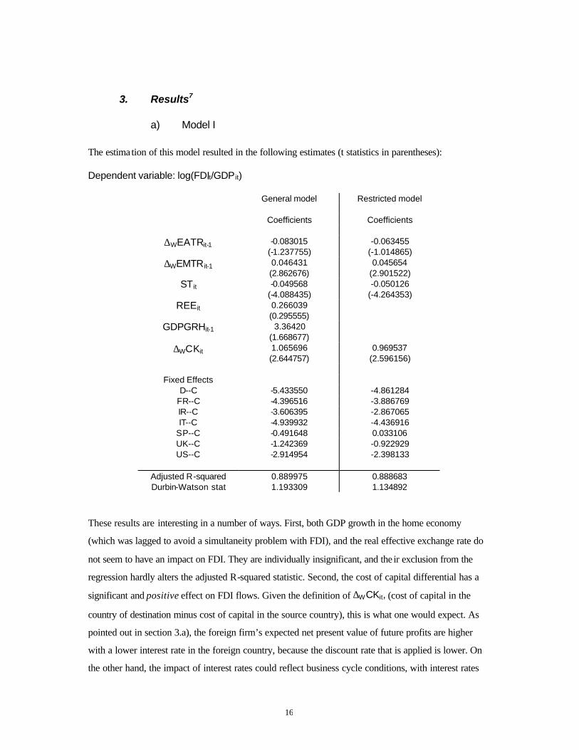
a) Model I The estimation of this model resulted in the following estimates (t statistics in parentheses): Dependent variable: log(FDIit/GDP it)

General model Restricted model Coefficients Coefficients

∆WEATRit-1 -0.083015 (-1.237755)

-0.063455 (-1.014865)

∆WEMTRit-1 0.046431 (2.862676)

0.045654 (2.901522)

STit -0.049568 (-4.088435)

-0.050126 (-4.264353)

REEit 0.266039 (0.295555)

GDPGRHit-1 3.36420 (1.668677)

∆WCKit 1.065696 (2.644757)

0.969537 (2.596156)

Fixed Effects

D--C -5.433550 -4.861284 FR--C -4.396516 -3.886769 IR--C -3.606395 -2.867065 IT--C -4.939932 -4.436916

SP--C -0.491648 0.033106 UK--C -1.242369 -0.922929 US--C -2.914954 -2.398133

Adjusted R-squared 0.889975 0.888683 Durbin-Watson stat 1.193309 1.134892

These results are interesting in a number of ways. First, both GDP growth in the home economy

(which was lagged to avoid a simultaneity problem with FDI), and the real effective exchange rate do

not seem to have an impact on FDI. They are individually insignificant, and the ir exclusion from the

regression hardly alters the adjusted R-squared statistic. Second, the cost of capital differential has a

significant and positive effect on FDI flows. Given the definition of ∆WCKit, (cost of capital in the

country of destination minus cost of capital in the source country), this is what one would expect. As

pointed out in section 3.a), the foreign firm’s expected net present value of future profits are higher

with a lower interest rate in the foreign country, because the discount rate that is applied is lower. On

the other hand, the impact of interest rates could reflect business cycle conditions, with interest rates

17

rising as the economy is growing faster. This would mean that ∆WCKit is correlated with GDP growth,

and could partially explain the insignificant coefficient on GDPGRHit-1. However, as one of the

advantages of panel data is to avoid multicollinearity between variables, this explanation is rather

unlikely. Also, from a theoretical point of view, business cycle conditions should affect foreign and

domestic firms symmetrically.

Turning to the different tax rates, the statutory rate is highly significant. The EMTR differential

is also significant, but has got the wrong sign. Finally, the EATR has got the right sign, but is

insignificant. Collinearity between the EATR and the statutory tax rate is possible, but again this

problem should have been reduced by panel data. The wrong sign on ∆WEMTRit-1 could possibly be

explained by the fact that one is dealing with a differential, and a political-economy argument. As the

variable is defined as home EMTR minus foreign EMTR, the differential can widen through either an

increase in home EMTR, or a reduction in foreign EMTR (or, less interestingly, both). If the latter is

the case, then EMTR could have fallen because of ‘too much’ (e.g. from a politicians point of view)

capital leaving the foreign country, and the subsequent reaction of policymakers8. However, it is not

clear whether such a mechanism is very likely.

There is an important caveat to the analysis conducted. First, the Durbin-Watson statistic is quite low,

which indicates serial correlation in the error terms. As in standard econometric theory, in a panel data

context this means that the coefficients cannot be estimated cons istently. This could mean that a

relevant explanatory variable was omitted. However, economic theory does not suggest any easy-to-

estimate variables other than those included. Factors such as consumer confidence (arguably the

driving force behind current US-American economic growth, which to a large extent is fuelled by

foreign capital imports) are difficult to estimate empirically. Another reason for serial correlation could

be the fact that FDI follows an auto-regressive process. Unfortunately, the inclus ion of a lagged

dependent variable in panel data models poses difficult econometric problems9.

7 All the results were obtained using Eviews. 8 This reaction would have to consist in an increase of the capital allowance, thus mainly affecting the EMTR, and not EATRs. A reduction of the statutory tax rate would mainly have an impact on the EATR, as pointed out above. 9 Consistent estimators can be obtained by using instrumental-variable methods. However, this requires special econometric software, such as DPD98 for Gauss.

18

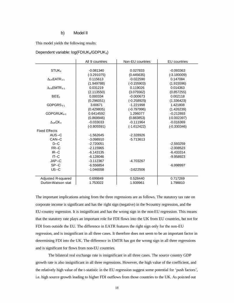
b) Model II This model yields the following results: Dependent variable: log(FDIUKit/GDPUKit)

All 9 countries Non-EU countries EU countries

STUKit -0.081340 (-3.291075)

0.027833 (0.445635)

-0.093363 (-3.180009)

∆UKEATR it-1 0.115613 (1.949788)

-0.022590 (-0.155903)

0.147084 (1.915596)

∆UKEMTR it-1 0.031219 (2.113550)

0.119026 (3.075562)

0.014363 (0.857255)

BEEit 0.000334 (0.296051)

-0.000673 (-0.258925)

0.002118 (1.336423)

GDPGRS it-1 3.60671 (0.429805)

-1.221998 (-0.797996)

1.421808 (1.426239)

GDPGRUKit-1 0.6414592 (0.869946)

1.296077 (0.883853)

-0.212893 (-0.002397)

∆UKCK it -0.033033 (-0.805591)

-0.111964 (-1.612422)

-0.016369 (-0.330346)

Fixed Effects AUS--C -1.562645 -2.328926 CAN--C -3.098910 -5.713613

D--C -2.720051 -2.593259 FR--C -2.115965 -2.008523 IR--C -6.143135 -6.433314 IT--C -6.128046 -9.958923

JAP--C -3.112367 -4.703267 SP--C -6.556854 -6.998997 US--C -1.046558 -3.622506

Adjusted R-squared 0.699849 0.528440 0.717269 Durbin-Watson stat 1.753022 1.939961 1.798810

The important implications arising from the three regressions are as follows. The statutory tax rate on

corporate income is significant and has the right sign (negative) in the 9-country regression, and the

EU-country regression. It is insignificant and has the wrong sign in the non-EU regression. This means

that the statutory rate plays an important role for FDI flows into the UK from EU countries, but not for

FDI from outside the EU. The difference in EATR features the right sign only for the non-EU

regression, and is insignificant in all three cases. It therefore does not seem to be an important factor in

determining FDI into the UK. The difference in EMTR has got the wrong sign in all three regressions

and is significant for flows from non-EU countries.

The bilateral real exchange rate is insignificant in all three cases. The source country GDP

growth rate is also insignificant in all three regressions. However, the high value of the coefficient, and

the relatively high value of the t-statistic in the EU regression suggest some potential for ‘push factors’,

i.e. high source growth leading to higher FDI outflows from those countries to the UK. As poin ted out

19

above, this would have to do with the existence of cash-constrained corporations in imperfect capital

markets. GDP growth in the UK, on the other hand, is clearly not significant for FDI inflows. Finally,

differences in the cost of capital do not seem to play an important role, as the coefficients are all

wrongly signed and insignificant.

Generally, the regression involving EU countries results in a much better fit (with and adjusted

R-squared of 0.717) than the regression involving non-EU countries. This is not very surprising given

that the EU countries form a relatively homogeneous economic area, and probably view the UK in a

similar way, which is clearly not the case for countries as different as Australia, Canada, Japan, and

the US. Therefore, it is much easier to fit a regression modelling the common response to different

variables of the former group of countries, than to unify the behaviour of the latter group within one

model.

More interestingly, the serial correlation in the error term of the EU regression is higher than

the serial correlation in the error term of the other group of countries. Again, this probably means the

omission of a relevant variable in the first regression, which has to be a factor common to the EU

economies but not to the non-EU economies. This could be the ongoing economic integration within the

EU. It is not difficult to imagine that this process does not proceed at a constant pace, but follows a

cycle, which could be driven by major political events on the European stage, such as the treaties of

Maastricht and Amsterdam. Such events could influence FDI flows within the EU, consequently

leading to correlations between those flows.

4. Limitations of the analysis Data problems . These concern mainly the data on FDI flows, which are often of poor quality, but also

the effective tax rates. As described in appendix I, several crucial assumptions have to be made in

order to be able to obtain aggregate rates. Most importantly, the composition of industries benefiting

from FDI flowing into the economy is assumed to be constant, which is clearly questionable.

Furthermore, issues of ‘tax planning’ (e.g. through transfer pricing or the repatriation of profits as a

royalty instead of a dividend) are neglected10.

The effective tax rate s feature relatively little variation, which reduces the efficiency of the

estimators. This could be one of the technical reasons for the relatively high number of insignificant

variables in the regressions.

Signs of a structural break in both series of FDI inflows around the late 1980s. This makes efficient

estimation considerably more difficult11.

10 Devereux and Freeman (1995). 11 The use of dummy variables to deal with this problem did not lead to any more satisfactory results.

20

5. Implications for the theories of FDI determination In part 3, four different models of FDI determination were presented: cost-of-capital, industrial

organisation, corporate investment, and portfolio theory. In the light of the preceding empirical

evidence, these models can be evaluated as follows. First, the cost-of-capital theory cannot be rejected.

In model I, the coefficient on interest rate differentials was significant, and positive. In a way, this can

be seen as a consequence of the Feldstein-Horioka (1980) result 12. Second, the regressions presented

do not shed a clear light on the industrial organisation-explanation, as no specific dynamic effects along

those lines were modelled. Third, corporate investment theory clearly plays a role, given the

significance of tax rate measures in the regressions. Fourth, portfolio theory is difficult to evaluate, as it

is consistent with any of the other explanations. The only hint that it might be relevant is the serial

correlation in the error term of the EU-country regression in model II. If this is due to European

integration, then such integration will lead to portfolio diversification of companies within the EU.

Looking at specific parameters, GDP growth and exchange rate effects are irrelevant. While the

insignificance of the former factor is somehow puzzling, the insignificance of the latter is predicted by

economic theory.

In all the regressions conducted, the statutory tax rate was consistently significantly and

negatively related to FDI flows, as one would expect. However, EATRs are always insignificant,

which is not the result predicted by economic theory, especially given its correlation with the statutory

tax rate. Finally, EMTRs are sometimes significant, but wrongly signed. This suggests the following

picture: the statutory tax rate plays an important role in determining FDI flows. This could be for three

reasons. First, investors might be imperfectly informed. In other words, they might not be able to

calculate the effective tax rates they will have to pay on an investment project, and thus use the

headline rate by default. However, it is not very plausible that investors should consistently behave in

such an irrational way. A second explanation is that statutory tax rate might act as a signal of business-

friendly policy by governments, accompanied by measures which were not included in the analysis.

Indeed, subsidies might play an important role as pointed out by C.H. Hahn13, who speaks of a ‘sheer

fight for investors via subsidies’.

12 Which roughly says that international capital markets are not perfectly integrated, implying that interest rate differentials between countries still obtain. 13 Chairman emeritus of Volkswagen, serves on various boards in North America and Europe.

21

The third, and most far-reaching explanation for the significance of the statutory tax rate is that the

latter might reflect the possibility of shifting profits between locations to benefit from a lower statutory

tax rate 14. This can actually explain all the features with regard to tax rates displayed in the

regressions, and is thus truly intriguing15. The argument proceeds in three steps. First observation: the

regression results show that the statutory tax rate plays an important role, while the EATR does not.

This indicates that the foreign direct investor seems to care about the statutory rate, but not about the

tax levied on an investment project earning economic rent. Second observation: the EMTR is often

significantly and positively related to FDI, i.e. a high EMTR implies a high FDI inflow. This means

that the investor is not concerned with a marginal project either. Third observation: as shown above and

in the appendix, a rise in the EMTR is usually due to a fall in the statutory tax rate, which is outweighed

by a reduction in capital allowances. In this case, a rise in the EMTR is equivalent to a reduction of the

statutory rate. Therefore, the positive correlation between FDI inflows and the EMTR really is a

negative relation between FDI inflows and the statutory rate (i.e. back to the first observation). Putting

those pieces together (and somewhat generalising) gives the following picture: the foreign direct

investor is not concerned with the effective tax rate on a marginal investment project, and he is not

concerned with the effective tax rate on an average investment project. In other words, he is not

concerned with any investment project whatsoever! The only thing he (or she) cares about is the low

statutory tax rate. What does this mean? This means that a considerable part of what is considered to

be FDI really is not FDI as defined by the OECD, i.e. taking control of a foreign company to run it

profitably. On the contrary: what one is dealing with are funds that are shifted to the place with the

lowest statutory tax rate and this clearly points to ‘tax planning’.

One could now argue whether this result is due to bad definitions and/or data management by

the OECD or the IMF, or whether it is due to the fact that investors will use any opportunity to reduce

their tax bill16. Unfortunately, there is neither time nor space to explore those matter further17.

6. Comparison with selected literature While the literature on the de terminants of FDI is very voluminous, there is not much evidence on the

impact of taxation on FDI. The results of two papers applying the EATRs and EMTRs used in this

essay are summarised briefly.

14 Devereux and Griffith (1996). 15 A personal note from the author: this ‘discovery’ was made in the late stages of writing this essay. It is related to a practice that was supposed to be ‘assumed away’ in the analysis: tax planning. However, this issue could be, and quite likely is, the key to most (all?) the ‘counterintuitive’ regression results obtained with respect to tax rates. On the other hand, it is a somehow disconcerting discovery after having spent a lot of time trying to get the regression results ‘predicted by economic theory’, without success. 16 One could also criticis e the construction of the EMTRs for mixing features of the tax system that should rather be left separated.

22

Devereux and Freeman (1995) use data on flows between seven countries for the period from 1984 to

1989, and a measure of the cost of capital. Looking at the decision of multinationals where to allocate a

given level of total investment, they find that taxation is generally insignificant. They speculate that this

might be due to measurement errors in the available data. Their result is relevant for multinational firms

genuinely interested in ‘true’ (i.e. following the OECD definition) FDI. As was shown above, with

aggregate data other factors come into play.

Devereux and Griffith (1996) analyse the locational decision of production using a panel of US

multinationals. Their results show that the EATR plays an important role in this decision, given that the

firm has already decided to locate production in Europe. They also find that there is some evidence that

the statutory tax rate plays an ‘independent and additional role in affecting the probability of locating in

a country.’ The latter result is confirmed by the analysis in this essay.

V. Conclusion The initial aim of this essay was to analyse the tax sensitivity of foreign direct investment. This

endeavour eventually succeeded, but in a rather unexpected way. Two panels were analysed

econometrically, one with data on total FDI inflows into 7 industrialised countries, the other with data

on FDI inflows into the UK from 9 OECD countries. At first glance, the results did not seem to fit the

theoretical predictions well: the statutory tax rate was significantly and negatively related to FDI

inflows, effective average tax rates were insignificant, and effective marginal tax rates were often

significantly but positively related to FDI inflows. Those features could partly be explained within the

traditional framework which regards FDI as funds being channelled into the investment project with the

highest economic rent. Such explanations are, e.g., a signalling function of the statutory tax rate.

However, this was not entirely satisfactory.

All the results concerning tax rates can be justified once one abandons the traditiona l

framework and takes into consideration the fact that FDI might be used as a tool by corporate

investors to channel profits to the places with the lowest statutory tax rates. This explains the positive

correlation between FDI and statutory rates, the nega tive correlation between FDI and effective

marginal tax rates, and the insignificance of effective average tax rates. However, it is important to

point out that these features were obtained for aggregate data, where FDI possibly includes capital

flows that should not be included in that category. Therefore, the evidence presented in this essay is

still consistent with firm-level data which reaches different conclusions.

17 Another interesting issue that cannot be pursued here is the fact that the welfare consequences from ‘true’ FDI could differ markedly from the welfare consequences of mere profit-shifting.

23

References Brainard, W. and J. Tobin (1992), ‘On the Internationalisation of Portfolios’, Oxford Economic Papers, vol. 44, pp. 533-65. Chennells, L. and R. Griffith (1997), Taxing Profits in a Changing World, London: The Institute for Fiscal Studies. Devereux, M.P. (ed.) (1996), The Economics of Tax Policy, Oxford: Oxford University Press. and H. Freeman (1995), ‘The Impact of Tax on Foreign Direct Investment: Empirical Evidence and the Implications for Tax Integration Schemes’, International Tax and Public Finance 2: 85-106. and R. Griffith (1996), ‘Taxes and the Location of Production: Evidence from a Panel of US Multinationals’, IFS Working Paper No. W96/14. and R. Griffith (1998), ‘The Taxation of Discrete Investment Choices’, IFS Working Paper No. W98/16. Dunning, J. H. (1993), Multinational Enterprises and the Global Economy, Wokingham, England/ Reading, Mass.: Addison Wesley. Froot, K., and J.C. Stein (1991), ‘Exchange Rates and Foreign Direct Investment: An Imperfect Capital Markets Approach.’ Quarterly Journal of Economics 106, pp. 1191-1217. Graham, E.M., and P.R. Krugman (1995), Foreign Direct Investment in the United States , Washingon, D.C.: Institute for International Economics. Hsiao, C. (1986), Analysis of Panel Data, Cambridge, England: Cambridge University Press. IMF (International Monetary Fund) (1996), Balance of Payments Statistics Yearbook , Washington, D.C.: International Monetary Fund. Lipsey, R.E. (1999), ‘The Role of Foreign Direct Investment in International Capital Flows’, in: M. Feldstein, International Capital Flows, Chicago: University of Chicago Press. OECD (Organisation for Economic Cooperation and Development) (1996), OECD Benchmark Definition of Foreign Direct Investment, 3rd ed., Paris: Organisation for Economic Cooperation and Development.

24

Appendix I - Technical Notes

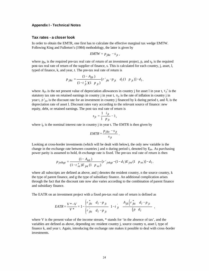
Tax rates - a closer look In order to obtain the EMTR, one first has to calculate the effective marginal tax wedge EMTW. Following King and Fullerton’s (1984) methodology, the latter is given by

EMTW p sjlkt jt= − ,

where pjkt is the required pre-tax real rate of return of an investment project, p, and sjt is the required post-tax real rate of return of the supplier of finance, s. This is calculated for each country, j, asset, l, typed of finance, k, and year, t. The pre-tax real rate of return is

pA

jlktjlt

jtr

jtjkt jt l jt l=

−

− +− + + −

( )

( )( )[ ' ( )]

1

1 11

τ πρ π δ π δ ,

where Ajlt is the net present value of depreciation allowances in country j for asset l in year t, τ jtr is the

statutory tax rate on retained earnings in country j in year t, πjt is the rate of inflation in country j in year t, ρ’jkt is the discount rate for an investment in country j financed by k during period t, and δl is the depreciation rate of asset l. Discount rates vary according to the relevant source of finance: new equity, debt, or retained earnings. The post-tax real rate of return is

si

jtjt

jt=

+

+−

1

11

π,

where ijt is the nominal interest rate in country j in year t. The EMTR is then given by

EMTRp s

sjlkt jt

jt=

−.

Looking at cross-border investments (which will be dealt with below), the only new variable is the change in the exchange rate between countries j and n during period t, denoted by Ejnt. As purchasing power parity is assumed to hold, th exchange rate is fixed. The pre-tax real rate of return is then

pA

EEjnlkgt

nlt

ntr

jnt ntjnkgt l jnt nt l=

−

− +− − + −

( )

( ) ( )[ ' ( ) ( )]

1

1 11 1

τ πρ δ π δ ,

where all subscripts are defined as above, and j denotes the resident country, n the source country, k the type of parent finance, and g the type of subsidiary finance. An additional complication arises through the fact that the discount rate now also varies according to the combination of parent finance and subsidiary finance. The EATR on an investment project with a fixed pre-tax real rate of return is defined as

( )( )

( )( )

EATRV V

V

A

p

jkt l jt

jkt l jtjt

jlt jkt l jt

l=

−= −

+ −

+ −− +

+ −

+

∗ ∗*

* ''1 1

ρ δ π

ρ δ πτ

ρ δ π

δ,

where V is the present value of the income stream, * stands for ‘in the absence of tax’, and the variables are defined as above, depending on: resident country j, source country n, asset l, type of finance k, and year t. Again, introducing the exchange rate makes it possible to deal with cross-border investments.

25

Effective exchange rates: definitions • nominal effective exchange rate index: ratio of an index of the period average exchange rate of the

currency in question to a weighted average of exchange rates for the currencies of selected countries

• real effective exchange rate index: nominal exchange rate index adjusted for relative movements in national price of cost indicators of the home country and selected countries

The weights used are attributed according to the trade share with the major trading partners.