The authors are grateful to Peter Orszag for many helpful comments and guidance in modeling the saver’s credit, to Jeff Rohaly for providing general oversight of the computer modeling work, and to Troy Kravitz for excellent research assistance. Views expressed do not necessarily reflect the views of the Urban Institute, its trustees, or its funders.

The AARP Public Policy Institute, formed in 1985, is part of the Policy and Strategy Group at AARP. One of the missions of the Institute is to foster research and analysis on public policy issues of importance to mid-life and older Americans. This publication represents part of that effort.

The views expressed herein are for information, debate, and discussion, and do not necessarily represent official policies of AARP.

© 2005, AARP. Reprinting with permission only. AARP, 601 E Street, NW., Washington, DC 20049 http://www.aarp.org/ppi

#2005-03

April 2005

The Effects of the Economic Growth and Tax Relief Reconciliation Act of 2001 on Retirement Savings and

Income Security

by

Leonard E. Burman The Urban Institute and the Tax Policy Center

William G. Gale

The Brookings Institution and the Tax Policy Center

Matthew Hall The Brookings Institution

i

TABLE OF CONTENTS

Table of Contents……………………………………………………………………………….….i Foreword……………………………………………………………………………………….…iii Executive Summary………………………………………………………………………………iv I. Introduction....................................................................................................................... 1 II. Data Sources ...................................................................................................................... 2 III. Federal Tax Incentives for Saving................................................................................... 3

A. Saving Incentive Rules Before EGTRRA............................................................... 3 1. Main Types of Pensions...................................................................................... 3 2. Defined Benefit Plans ......................................................................................... 5 3. Defined Contribution Plans ................................................................................ 5

a. 401(k) Plans .................................................................................................... 6 b. 403(b) and 457 Plans ...................................................................................... 6 c. Keogh Accounts.............................................................................................. 6 d. IRAs ................................................................................................................ 7 e. Simplified Employee Pensions (SEPs) ........................................................... 9 f. SIMPLE Retirement Plans.............................................................................. 9

B. Effect of EGTRRA on Savings Incentives ............................................................. 9 1. Traditional Defined Benefit Plans .................................................................... 11 2. Defined Contribution Plans (including SEPs) .................................................. 11 3. 401(k) Plans (and related plans, including Keogh)........................................... 11 4. IRAs .................................................................................................................. 11 5. Coverdell Education Savings Accounts (ESAs) ............................................... 11 6. Saver’s Tax Credit ............................................................................................ 12 7. Small Business Tax Credit for New Retirement Plan Expenses....................... 12 8. SARSEP-IRAs .................................................................................................. 12 9. SIMPLE Retirement Plans................................................................................ 12

IV. Effects of EGTRRA on Private and National Saving .................................................. 13 A. Effects on Private Saving...................................................................................... 13

1. Changes in Effective Marginal Tax Rates ........................................................ 13 2. Income Tax Changes and Education and Retirement Saving Incentives ......... 14 3. Estate Tax Changes........................................................................................... 15 4. Overall Effects on Private Saving..................................................................... 15

B. Effects on Public and National Saving ................................................................. 16 1. Effects on Public Saving................................................................................... 16 2. Net Effects on National Saving......................................................................... 16

V. Distribution of Pension and IRA Tax Benefits Before and After EGTRRA............. 17 A. Distribution of Defined Contribution Pension and IRA Tax Benefits before

EGTRRA............................................................................................................... 18 B. Pension Tax Benefits Under EGTRRA ................................................................ 20 C. Distribution of Pension Tax Benefits by Age ....................................................... 22 D. Two Policy Options .............................................................................................. 22

VI. Summary and Conclusions............................................................................................. 23

ii

VII. References........................................................................................................................ 25 VIII. Tables ............................................................................................................................... 28 IX. Figures.............................................................................................................................. 49 X. Appendix: Modeling Savings Tax Incentives ............................................................... 51

A. Pension Contribution and Coverage ..................................................................... 51 1. Estimation ......................................................................................................... 51 2. Imputation ......................................................................................................... 53 3. Calculating Gross Wages.................................................................................. 54

B. IRA Participation and Contributions .................................................................... 55 C. Modeling the Saver’s Credit and Alternatives...................................................... 56 D. Simulating Alternative Policies ............................................................................ 57 E. Calculating the Present Value of Tax Benefits from IRAs and Pensions............. 57

1. Assumptions for Calculations ........................................................................... 58 XI. Glossary ........................................................................................................................... 59

iii

FOREWORD

As the baby boomers approach their retirement years, the media routinely report dire

warnings of the fiscal catastrophes awaiting the nation if boomers and Americans generally do not change their spendthrift ways and start saving more for their own retirement. These warnings appear to have had little effect, since the personal saving rate has declined steadily over two decades, dropping from about 11 percent of disposable personal income in the early 1980s to 1.4 percent in 2003 according to the National Income and Product Accounts (NIPA) data, and even into negative territory (in 2000) according to Federal Reserve Board (FRB) Flow of Funds Accounts (FFA) data.

The NIPA and FFA measures of saving may differ because of differences in definitions

of saving, but they emphatically agree that the direction has been steadily downward, and that as a nation we are saving too little to sustain our level of consumption. This is particularly true in view of the large future public spending increases necessitated by the retirement of the boomers over the next 25 years.

We have frequently looked to government to stimulate private saving, usually through tax

incentives for such things as home purchases, for retirement saving, for health insurance, and for education. At the same time, however, many experts have argued that the best way to increase national saving is to reduce federal deficits, an argument that was heard often in the 1980s and 1990s, when the nation struggled to reduce federal budget deficits never before seen in peacetime. That 15-year struggle ultimately bore fruit, as the federal deficit was eliminated and the federal budget realized a string of four successive budget surpluses from 1998 through 2001.

In 2001, the Bush Administration proposed and Congress enacted the Economic Growth

and Tax Reform Reconciliation Act (EGTRRA), which was in part explicitly intended to increase national saving by means of liberalized contributions to defined contribution pension plans and Individual Retirement Accounts and the reduction and subsequent repeal of the estate tax. However, as this paper by Leonard Burman of the Urban Institute and William Gale and Matthew Hall of the Brookings Institution shows, the net effect of EGTRRA will be to increase private saving only at the expense of increasing public borrowing (i.e., increased federal budget deficits), resulting in an overall decline in national saving of as much as one percent of GDP. EGTRRA’s tax benefits were also largely bestowed on the highest-income fifth of the population, a group more likely to simply swap taxable for nontaxable saving when presented with new tax benefits. Consequently, less new saving would be generated than if the tax benefits were more targeted on low- and moderate-income families.

John R. Gist Associate Director AARP Public Policy Institute

iv

Executive Summary Introduction Policymakers have frequently turned to tax policy to stimulate private saving. For

example, the Economic Growth and Tax Relief Reconciliation Act of 2001 (EGTRRA) introduced substantial cuts in income taxes, reductions and eventual repeal of the estate tax, and numerous incentives for increased private saving. EGTRRA is likely to affect both private and national saving through many channels.

Purpose This report examines the effects of EGTRRA on private and national saving and on the

distribution of federal tax benefits for saving. Methodology The study uses the Tax Policy Center’s microsimulation tax model. The principal data

source for information about type of pension, pension participation, and contributions by employers and employees is the Federal Reserve Board of Governors’ Survey of Consumer Finances (SCF) for 2001. The SCF is a stratified sample of about 4,400 households with detailed data on wealth and savings. Our source for income tax information is the 1999 public use file (PUF) released by the Statistics on Income Division of the Internal Revenue Service. This file contains detailed information about income and deductions as reported on individual income tax returns for a stratified sample of over 100,000 returns. That dataset is augmented with information from the 2000 Current Population Survey using a statistical matching process

The tax model database on to which we impute the savings variables is an enhanced

version of the 1999 public-use file (PUF) containing 132,108 records and produced by the Statistics of Income (SOI) Division of the Internal Revenue Service (IRS). For the years from 2000 to 2013, we "age" the data based on forecasts and projections for the growth in various types of income from the Congressional Budget Office (CBO), the growth in the number of tax returns from the IRS, and the demographic composition of the population from the Bureau of the Census. Actual 2000 and 2001 data are used when they are available. A two-step process produces a representative sample of the filing and non-filing population in years beyond 1999. First, the dollar amounts for income, adjustments, deductions and credits on each record are inflated by their appropriate per capita forecasted growth rates. For the major income sources such as wages, capital gains, and various types of non-wage income such as interest, dividends, social security income and others, specific forecasts are used for per capita growth. Most other items are assumed to grow at CBO's projected per capita personal income growth rate. In the second stage of the extrapolation process, the weights on each record are adjusted using a linear programming algorithm to ensure that the major income items, adjustments, and deductions match aggregate targets. For years beyond 1999 we do not target distributions for any item; wages and salaries, for example, grow at the same per capita rate regardless of income.

v

Findings While the new tax incentives may induce some increase in private saving, the increased

private saving is likely to be more than offset by the increase in deficits (reduced public saving). As a result, the net effect is likely to be a reduction in national saving that could be as large as 1 percent of GDP from 2002 to 2011.

Overall, the income and estate tax changes should at most raise private saving by about

0.5 percent of GDP between 2002 and 2011. Unfortunately, those gains are more than negated by the higher deficits arising from the fact that EGTRRA was entirely debt-financed. The modeling results suggest that public borrowing will increase by more than three times as much as the increase in private savings over the decade. As a result, EGTRRA is likely to cut national saving—the sum of private and public saving—by more than 1 percent of GDP. Even if private saving is highly responsive to tax changes, the entire package is likely to reduce national saving by at least 0.6 percent of GDP.

We find that pension and IRA tax benefits are fairly concentrated at higher income levels.

About 70 percent of such tax benefits accrued to the highest-income 20 percent of tax filing units in 2001, before the EGTRRA tax changes took effect, and almost 47 percent went to the top 10 percent. Because eligibility for IRAs was subject to income limits, they are less skewed with income than contributions to defined contribution (DC) plans. Still, more than 60 percent of IRA tax benefits accrue to the top 20 percent of households.

The EGTRRA pension and IRA provisions were less skewed by income in 2003 than

preexisting benefits, because of the saver’s tax credit, which primarily benefits those in the bottom half of the income distribution, and because many of the limit increases are phased-in slowly. In 2010, however, when EGTRRA is fully phased-in, the pension and IRA tax benefits are much more concentrated. About 75 percent of the benefits accrue to those in the top quintile, and 56 percent to those in the top 10 percent. This is slightly more skewed than the distribution of all EGTRRA tax changes in 2010, although the other EGTRRA provisions are far more valuable for people with very high income (95th percentile and above) than the pension expansions. The skew of the pension provisions would be lessened if the saver’s credit, which only took effect in 2002, were extended rather than being allowed to expire in 2006.

Two options under consideration would have very different effects on the distribution of

tax benefits. One option would accelerate the scheduled phase-in of EGTRRA pension and IRA provisions to 2004. The benefits of such a plan would be heavily skewed towards high-income taxpayers—more than half of the benefits would go to the top 10 percent. Such a policy is unlikely to have much effect on personal saving because high-income people are most likely to simply swap taxable for nontaxable saving when presented with new tax benefits. In contrast, another alternative—making the saver’s credit refundable—would have very different effects. About 87 percent of the tax cuts would go to the bottom three quintiles. For these people, additional retirement saving almost surely comes out of reduced consumption because they have

vi

little in the way of liquid financial assets to shift. Moreover, these households have the most to gain in retirement security from increased saving.

Conclusions This paper examined how the 2001 tax changes affect saving and the distribution of

income tax liabilities. In addition to the direct saving tax incentives, the 2001 act could affect saving indirectly through several avenues—most notably, the reduction in marginal income tax rates, the repeal of the estate tax, and the increase in public debt. Overall, the income and estate tax changes could at most raise private saving by about 0.5 percent of GDP between 2002 and 2011. Unfortunately, those gains are more than negated by the higher deficits arising from the fact that EGTRRA was entirely debt-financed. Public borrowing will increase by more than three times as much as the increase in private savings over the decade. As a result, EGTRRA is likely to cut national saving—the sum of private and public saving—by more than 1 percent of GDP. Even if private saving is highly responsive to tax changes, the entire package is likely to reduce national saving by at least 0.6 percent of GDP.

1

I. Introduction

The ability of individuals and societies to maintain or improve their living standards over time depends on their willingness to save. At an individual level, people need to accumulate sufficient wealth to finance an adequate retirement, protect against economic risks, and so on. At an aggregate level, society needs to save enough to provide the capital (financial, physical, and human) that is needed to raise future productivity and in turn raise wages and living standards. Both of these concerns are becoming increasingly important; the baby boomers are starting to retire and they are living longer. All the while, private and national saving rates have remained low.

Policymakers have frequently turned to tax policy to stimulate private saving. For

example, the Economic Growth and Tax Relief Reconciliation Act of 2001 (EGTRRA) introduced substantial cuts in income taxes, reductions and eventual repeal of the estate tax, and numerous incentives to increase private saving. EGTRRA is likely to affect both private and national saving through many channels.

This report examines the effects of EGTRRA on private and national saving and on the

distribution of federal tax benefits for saving. It finds that, while the new tax incentives may induce some increase in private saving, that increase is likely to be more than offset by reduced public saving. As a result, the net effect is likely to be a reduction in national saving that could be as large as 1 percent of GDP from 2002 to 2011.

Pension and individual retirement account (IRA) tax benefits are mostly concentrated

among high-income taxpayers for two reasons. First, these taxpayers can afford to save. Second, they face the highest marginal tax rates and thus stand to gain the most from tax deductions and exclusion. The EGTRRA changes, when fully phased in, will simply reinforce that pattern, because the increase in contribution limits primarily benefits high-income people who are constrained by the current limits. If the new, temporary, saver’s tax credit were extended, it would partially offset this skew because it is targeted at low- and middle-income households. In addition, if the saver’s credit were made refundable—that is, available to tax filers regardless of their income tax liability—it would provide a substantial and well-targeted tax benefit to people in the bottom half of the income distribution.

The plan of the report is as follows. Section II describes the underlying tax model and

data sources employed. Section III describes saving rules that existed before EGTRRA took effect and the changes introduced in EGTRRA. Section IV provides estimates of the effects of EGTRRA on private and national saving. Section V examines the distribution of federal tax benefits for saving under pre- and post-EGTRRA law. Section VI provides a summary and conclusions. A technical appendix describes our methodology for measuring the benefit of pension and IRA tax provisions.

2

II. Data Sources

The analysis reported below requires measures of income tax rates and retirement saving in various forms by income, age, and other individual characteristics. Our principal data source for information about type of pension, pension participation, and contributions by employers and employees is the Federal Reserve Board of Governors’ Survey of Consumer Finances (SCF) for 2001. The SCF is a stratified sample of about 4,400 households, with detailed data on wealth and savings. Our source for income tax information is the 1999 Public Use File (PUF) released by the Statistics on Income Division of the Internal Revenue Service. This file contains detailed information about income and deductions as reported on individual income tax returns for a stratified sample of over 100,000 returns. That data set is augmented with information from the 2000 Current Population Survey using a statistical matching process to include information about age of taxpayer (and spouse on joint returns), the split of earnings between head and spouse on joint returns, and transfer payments not reported on income tax returns. To measure eligibility and contributions to individual retirement accounts, we use pooled data from the 1984, 1990, 1992, and 1996 Survey of Income and Program Participation (SIPP) samples. We selected individuals who were full-time workers, not self-employed, and between 25 and 55 years of age. We dropped records from which tax, IRA, or pension data were missing, yielding a sample of 40,188 households.

SIPP participants are reinterviewed every four months for two years, creating new

“waves” of data with additional information. Data on IRAs were derived from wave 7, so they refer to the tax year following the sample year—so the 1996 SIPP yields IRA data for tax year 1997. We calibrate our estimates for IRA participation and contributions to match summary data published by the Internal Revenue Service (IRS) (Sailer and Nutter, forthcoming).

The tax model database onto which we impute the savings variables is an enhanced

version of the 1999 PUF containing 132,108 records and produced by the Statistics of Income (SOI) Division of the IRS. The detailed information in the PUF from federal individual income tax returns filed in the 1999 calendar year is augmented with additional information on demographics and sources of income through a constrained statistical match with the March 2000 Current Population Survey (CPS) of the U.S. Census Bureau. This statistical match also generates a sample of individuals who do not file income tax returns (nonfilers).

For the years from 2000 to 2013, we "age" the data on the basis of forecasts and

projections for the growth in various types of income from the Congressional Budget Office (CBO), the growth in the number of tax returns from the IRS, and the demographic composition of the population from the Bureau of the Census. We use actual 2000 and 2001 data when they are available. A two-step process produces a representative sample of the filing and non-filing population in years beyond 1999. First, the dollar amounts for income, adjustments, deductions, and credits on each record are inflated by their appropriate per capita forecasted growth rates. For the major income sources such as wages, capital gains, and various types of non-wage income such as interest, dividends, Social Security income, and others, we have specific forecasts for per capita growth. Most other items are assumed to grow at CBO's projected per capita personal income growth rate. In the second stage of the extrapolation process, the weights on each record are adjusted using a linear programming algorithm to ensure that the major

3

income items, adjustments, and deductions match aggregate targets. For years beyond 1999 we do not target distributions for any item; wages and salaries, for example, grow at the same per capita rate regardless of income.

For the purposes of projecting pension and other retirement savings, we rely on this two-

stage aging and extrapolation process to predict our explanatory variables for future years. The procedure for imputing pension and retirement savings variables is detailed in the appendix.

III. Federal Tax Incentives for Saving

This section describes the tax rules that applied to savings before EGTRRA, and how that legislation expanded incentives for saving.

A. Saving Incentive Rules Before EGTRRA

1. Main Types of Pensions

The two main types of tax-favored retirement savings accounts are treated differently in the tax and labor laws. The first type—traditional pension benefits, commonly called defined benefit (DB) plans—are paid out to workers as an annuity by their respective companies upon retirement.1 These retirement benefits are funded by tax-deductible contributions to an employee pension fund, which is required by federal law to remain in actuarial balance. Federal regulation in this type of retirement savings account is directed toward “vesting rights” of workers (the legal rights of workers to the benefits accrued in their names), insurance of the guaranteed benefits in case of corporate insolvency, and limitations on the percentage of total compensation that comes via this tax-preferred payment method.2

The second type of retirement plan, known as a defined contribution (DC) plan, is

composed of savings accounts that are funded by the individuals themselves. Although they were originally created in order to allow the self-employed and the employed with no pension benefits to use the same tax-preferred method to fund their own retirement needs, these accounts differ in many respects from defined benefit plans. Account balances need not be used to purchase an annuity upon distribution, and no benefits are guaranteed because the individuals own the account and fund some or all of it themselves. Federal regulation of the typical defined contribution plan is aimed at limiting the contribution to tax-preferred accounts, establishing

1 A defined benefit (DB) pension plan typically pays its benefit in the form of a life annuity, which pays a

periodic fixed benefit to the recipient until death. By law, DB plan participants must be offered the choice of a joint and survivor annuity, in which the surviving spouse continues to receive a portion of benefits after the participant dies. To choose instead a single life annuity (with no spousal benefits), the spouse must consent. Increasingly, DB plan participants are being offered the option of receiving their benefits in the form of a lump sum rather than an annuity.

2 Defined benefit pension plans are regulated not only under the tax law but also by the Employee Retirement

Income Security Act of 1974 (ERISA). ERISA requires employers to provide participants and beneficiaries with adequate information regarding their plans, protect plan funds and manage them prudently, and ensure that participants who qualify receive their benefits.

4

vesting rights of employees to contributions by their employers to the accounts, and encouraging (through nondiscrimination laws) employers to make such accounts available to large parts of their workforce.

Nondiscrimination rules play an important role in qualified plans, and they are quite

complex. The provisions prevent more than an allowable percentage of contributions by employers on behalf of their employees from going to “highly compensated” employees as opposed to “rank-and-file” employees. Additionally, the nondiscrimination rules are set up to regulate employer eligibility rules so that at least a minimum number of rank-and-file workers receive coverage.

Current law limits the benefits qualified pension plans may provide to highly

compensated employees (HCEs, basically defined in 2003 as those earning $90,000 or more) relative to rank-and-file workers, known as non-highly compensated employees (NHCEs). One requirement hinges on coverage rates. This requirement can be met if the share of rank-and-file workers covered is at least 70 percent of the share of HCE workers covered.3 For example, if all HCEs are covered, 70 percent of rank-and-file workers would need to be covered.

An additional set of tests applies specifically to 401(k) and similar defined contribution

plans. Under these tests, the share of compensation contributed by HCEs is limited by the share of compensation contributed by rank-and-file workers. For example, if the average contribution rate for rank-and-file workers is between 2 and 8 percent of salary, the average HCE contribution rate may not be more than 2 percentage points higher.4 Safe harbor rules allow firms to avoid these tests by offering specific patterns of 401(k) employer matching or nonmatching contributions; a plan following the safe harbor design satisfies the test regardless of actual take-up behavior.

A variety of other rules apply as well, some making the allowable pattern of contributions

more progressive and some making it less progressive. The “permitted disparity” rules allow higher contributions for highly compensated employees, in a manner that was intended to reflect the offsetting progressivity of social security benefits. The “cross-testing” rules allow higher contributions for older workers.5 The “top-heavy” rules require plans in which more than 60 percent of benefits accrue to “key” employees (such as certain executives and owners) to provide a minimum contribution equal to 3 percent of compensation to rank-and-file workers.

3 This is the so-called ratio percentage test. An alternative way of meeting the coverage requirement is through

the average benefits test. For a description of these tests, see Orszag and Stein (2001). 4 If the average contribution rate for NHCEs is less than 2 percent, the average HCE contribution rate is limited

to no more than 200 percent of the average NHCE contribution rate. If the NHCE average contribution rate is over 8 percent, the HCE average contribution rate can be no more than 125 percent of the NHCE average rate. Two similar and parallel tests (the actual deferral percentage (ADP) test and the actual contribution percentage (ACP) test) evaluate employee pre-tax contributions (ADP test) and the combination of employer contributions and employee after-tax contributions (ACP test).

5 Orszag and Stein (2001) give examples of how the cross-testing rules can be used to subvert the intent of the

nondiscrimination rules.

5

The administrative burden of complying with nondiscrimination rules spawned an entire

separate set of rules for small employers who wish to implement a pension plan. These plans, described later, are allowed a “safe harbor” exception from the nondiscrimination rules if employers contribute at least a specified percentage of earned income to all eligible employees’ accounts irrespective of the employees’ elective contributions.

2. Defined Benefit Plans

In a defined benefit plan, the primary advantage to the worker is the elimination of many kinds of risk. The Pension Benefit Guarantee Corporation (PBGC) insures most defined benefit pension plans.6 Because the pension plans are insured, the employees are guaranteed a monthly benefit in retirement even if the employer goes bankrupt. The requirement of maintaining actuarial balance in order to pay a guaranteed annuity removes investment risk from the employee and puts that risk on the employer, who is presumably better able to manage it. Finally, the most significant way an annuity diminishes risk is by eliminating the risk of outliving savings. Again, this risk is significant for the individual worker but less so for the corporation that pools employees in a pension fund.

Pre-EGTRRA laws not only insured approved company pension plans and required that

the fund maintain actuarial balance but also limited the maximum benefit that could be paid annually to the lesser of the average salary in the employee’s three highest-paid consecutive years (annual salary for the purpose of this computation was limited to $170,000 in 2001) or $140,000 (in 2001).7

Employer contributions to the employee pension fund were deductible from both income

and payroll taxes as long as the contributions did not exceed those that were actuarially necessary to fully fund the maximum allowable benefit.

3. Defined Contribution Plans

Defined contribution plans refer to a number of plans that involve retirement accounts held by employees. Either employers or employees (or both) may contribute to these accounts, depending on the plan type. Unlike defined benefit plans, in which federal regulations apply to the ultimate benefits, the guidelines for defined contribution plans focus on how much compensation can be deferred, without regard to the ultimate benefits that will be conferred.

Under pre-EGTRRA law, in 2000 an addition to a participant’s plan (including both

employer and employee contributions) could not exceed the lesser of $30,000 or 25 percent of

6 PBGC covers the benefits in all private defined benefit plans up to established limits. State and local

employees are not covered because their employers’ plans are exempt from ERISA. 7 All contribution and benefit limits and income thresholds for employer plans are indexed for inflation,

generally in round number increments. For example, contributions and benefit limits generally increase in $5,000 increments, and adjustments to income thresholds occur in $10,000 increments. In contrast, before enactment of EGTRRA, limits for contributions to individual retirement accounts were not indexed to inflation.

6

the first $170,000 of earned income. The contribution limit increased to $35,000 in 2001 because of inflation indexing. Other contribution requirements and limitations existed that were specific to different types of defined contribution plans.

There are several kinds of defined contribution plans, including the 401(k) plan, the

403(b) plan, 457 plans, the IRA, the SIMPLE (Savings Incentive Match Plan for Employees) retirement plan, the Simplified Employee Pension (SEP), and the Keogh Account.

a. 401(k) Plans

The 401(k) plan, named after the tax code section that authorized it, allows employees of for-profit private entities to defer compensation into retirement plans and allows employers to make additional contributions—as automatic contributions, matching contributions, or a combination of both. Under pre-EGTRRA law, an employee could contribute up to $10,500 (indexed in $500 increments) as deferred income in the year 2000 . Excess contributions were considered normal income and were taxed accordingly. Employers could make additional contributions subject to an overall limitation on contributions to defined contribution plans ($35,000 in 2001). Employers could place lower limits on the amount contributed by employees and the employer’s matching contributions.

A “safe harbor” version of the 401(k) plan was created for small employers as a way to

reduce the administrative costs of meeting nondiscrimination requirements. It was extended, however, as an option to all employers. The employer in a safe harbor 401(k) plan must either offer a 100 percent match on employee contributions up to the first 3 percent of compensation and a 50 percent match on the next 2 percent of compensation, or an automatic (nonmatching) 3 percent of compensation of all eligible employees.

The contribution is deductible subject to the contribution limit for the employee. The

employer match is not considered income to the employee in the year the contribution is made. Withdrawals attributable to elective contributions cannot be made unless one of the following conditions is satisfied: (1) separation of service, death, or disability; (2) termination of the plan with no successor; (3) attainment of the age of 59 ½; or (4) hardship. The distribution that meets the requirements above is subject to income tax as any other compensation in that period. Excess contributions by employers on behalf of employees are subject to a 10 percent penalty.

b. 403(b) and 457 Plans

Separate code sections govern defined contribution plans similar to 401(k) plans that are offered by tax-exempt entities (section 403(b)) and state and local governments (section 457). Pre-EGTRRA, the rules governing these plans were similar to, but somewhat less restrictive than, those that applied to for-profit private employers.

c. Keogh Accounts

Self-employed persons can create a Keogh Account to act as their own pension plan. It is subject to the same rules as a 401(k) in terms of deferral of compensation, deductibility, distribution, and taxation on distributions. Earned income for a self-employed person is income

7

from that person’s business that is subject to the self-employment tax minus the 50 percent deduction of self-employment tax and the allowable deductions for contributions to the retirement plans on behalf of that individual.

d. IRAs

Individual retirement arrangements, also known as individual retirement accounts (IRAs), are tax-preferred retirement savings accounts that allow individuals with earned income (defined as salary or wages plus alimony received) and their spouses to deduct from gross income some portion of contributions or distributions. Traditional IRAs qualify for tax treatment similar to elective contributions to deferred compensation plans offered by employers, although some variants are subject to different tax treatment, as described below.

There are four general types of IRA: the traditional, the Roth, the nondeductible, and the

education IRA. Additionally, there are variations of the traditional IRA for self-employed workers and employees of small firms that are subject to most traditional IRA rules.

(1) Traditional IRA

Under pre-EGTRRA law, an individual under the age of 70 ½ could set aside earnings of up to $2,000 and deduct part or all of them from adjusted gross income (AGI). How much, if any, of a contribution was deductible depended on whether the individual or a spouse participated in an employer-sponsored pension plan, and on income. Eligibility for deductible IRA contributions phased out with income for taxpayers with access to an employer-sponsored plan. In 2000, the phaseout range was $52,000 to $62,000 for married taxpayers who file joint returns, $32,000 to $42,000 for singles and heads of household, and $0 to $10,000 for married couples who file separate returns. The beginning of the phaseout range is scheduled to increase over time (see table 1), to $80,000 for married filing joint returns in 2007 and $50,000 for singles and head of household in 2005. In 2007, the size of the phaseout range for married returns also doubles, to $20,000. The phaseout range for a married taxpayer filing a joint return without access to an employer plan whose spouse is covered by an employer plan is $150,000 to $160,000. Neither the income thresholds nor the maximum contribution amount is indexed for inflation.

Withdrawals must begin by age 70 ½, and the frequency and size of distributions must be

such that all funds are withdrawn by the end of the expected lifetime of the individual (complicated rules govern the amount and speed of withdrawals). Failure to withdraw enough invokes a 50 percent penalty on the difference between the minimum required distribution and the actual distribution, which can be waived if the mistake is due to “reasonable error” and is corrected. Early distributions, defined as withdrawals before age 59 ½, are subject to a 10 percent penalty. This penalty is void under certain circumstances, including the following: (1) the withdrawal is used by unemployed individuals (receiving unemployment compensation for 12 weeks) to pay medical insurance premiums; (2) the withdrawal is used to pay for higher education expenses (including books, fees, and supplies) of a dependent, spouse, or grandchild; or (3) the withdrawal (up to $10,000) is used to buy a first-time primary residence. IRA holders may take all or part of their balance as an annuity at any age. Distributions are generally subject to income tax.

8

(2) Roth IRA

The Roth IRA is different from the traditional IRA in several respects, the most important being deductibility rules and the absence of minimum withdrawal requirements. Moreover, there is no age limit for contribution to a Roth IRA, and contribution limits are different from those that apply to a traditional IRA. In 2000 the limit for total contributions to all types of IRAs was $2,000 per year. The maximum contribution to a Roth IRA phased out in 2000 over the following income ranges: $95,000 to $110,000 for single and head of household returns, $150,000 to $160,000 for married filing joint returns, and $0 to $10,000 for married filing separate returns.

Contributions to a Roth IRA are not deductible, but qualified distributions are tax-free. In

general, a withdrawal is a “qualified distribution” if taken at least five years after the initial contribution and if the account owner reaches age 59 ½, is disabled, or spends the proceeds to purchase a primary residence (subject to the same rules as apply to a traditional IRA). In addition, withdrawals made by a beneficiary upon death are not subject to the penalty. Other withdrawals are subject to a 10 percent penalty.

(3) Nondeductible IRAs

Any individual may contribute to a nondeductible IRA, subject to the constraint that the total contributions to deductible, nondeductible, and Roth IRAs may not exceed $2,000 in a year. Contributions to a nondeductible IRA are not deductible from income, but earnings are not taxable until withdrawal. Distributions are taxable in proportion to the earnings in the IRA account. Early nonqualifying distributions, defined similarly to those for traditional IRAs, are subject to a 10 percent penalty.

(4) Education IRA

The “Roth IRA of education saving,” the education IRA (now called the Coverdell Education Savings Account (ESA)), allows certain filers to contribute up to $500 (pre-EGTRRA, not indexed for inflation) per beneficiary per year toward postsecondary educational expenses for said beneficiary. The beneficiary must be under 18, and the annual sum of all contributions made on his or her behalf may not exceed $500. The contribution limit is subject to the same adjusted gross income (AGI) phaseout by filing status that applies to a Roth IRA, except that married taxpayers filing separate returns cannot contribute at all. The contribution limit is not affected by contributions to other IRAs.

Contributions to an education IRA are not deductible, and qualifying withdrawals are not

taxable. (Pre-EGTRRA law required that qualifying withdrawals be used for postsecondary educational expenses incurred by the beneficiary.) A qualifying distribution cannot be taken in the same year as the Hope credit or Lifelong Learning credit. Nonqualifying withdrawals are subject to a 10 percent penalty. In addition, the earnings portion of a nonqualifying withdrawal is included in gross income. (The earnings share is defined as 1 minus the ratio of total contributions to the account balance multiplied by the amount of the nonqualifying distribution.)

9

e. Simplified Employee Pensions (SEPs)

A Simplified Employee Pension is a defined contribution pension plan in which contributions are made to employees’ IRAs, called SEP-IRAs. SEP-IRAs are subject to the same limits that apply to other defined contribution plans: in 2001, annual contributions could not exceed the lesser of $35,000 or 15 percent of the first $170,000 of compensation. Employers generally have to contribute the same percentage of salary to all qualifying employees’ SEP-IRAs. Qualifying employees include those who have reached age 21, have worked for the employer for three of the past five years, and have earned at least $450 (in 2001). All contributions are fully vested. Subject to these constraints, the general nondiscrimination rules do not apply to SEP-IRAs.

f. SIMPLE Retirement Plans

Small employers may maintain SIMPLE retirement plans rather than the 401(k) plans that most large employers use. The employer must have fewer than 100 employees receiving at least $5,000 in compensation. The employer may not maintain any other employer-sponsored retirement plan for the same employees to whom it offers the SIMPLE plan.

SIMPLE plans may be either an IRA for each employee or a 401(k). Employees may

contribute up to $6,000 (indexed for inflation). The contribution is treated as a qualifying elective deferral. The employer must either provide a 100 percent match on contributions up to 3 percent of compensation or make an automatic nonelective contribution equal to 2 percent of compensation. Compensation for purposes of the matching contribution is limited to $170,000. An employer is permitted to reduce the matching contribution to a SIMPLE-IRA to as little as 1 percent of compensation, but not in more than two out of every five years. Contributions to a SIMPLE-IRA are immediately vested.

A SIMPLE-IRA is exempt from nondiscrimination rules that apply to qualified

retirement plans. A SIMPLE-401(k) is exempt from the special nondiscrimination rules applicable to 401(k) plans but is subject to other rules that govern qualified employer plans.

SIMPLE plans replaced Salary Reduction SEPs, or SARSEPs, which were eliminated in

1997. Plans established before 1997 were grandfathered and may admit new employees.

B. Effect of EGTRRA on Savings Incentives

Under EGTRRA, the highest income tax rates were scheduled to fall by varying amounts over time. When fully phased in, the top rate falls from 39.6 percent to 35 percent. (See table 2.) The 28, 31, and 36 percent rates all fall by three percentage points. All four rates were to be reduced by 0.5 percentage points on July 1, 2001, and January 1, 2002, and one percentage point at the beginning of 2004. In 2006, the lowest three rates were supposed to fall by another percentage point while the top rate will fall by 2.6 percentage points. The Jobs and Growth Tax Relief Reconciliation Act of 2003 (JGTRRA) accelerated the 2004 and 2006 changes to 2003. Thus, the rate reductions for taxpayers at all income levels are fully effective beginning with tax year 2003.

10

A new 10 percent tax bracket is carved out of the 15 percent bracket. Whereas the cuts in the highest income tax rates originally phased in slowly over time, the 10 percent bracket was made available immediately. Beginning in 2001, the new bracket applies to the first $12,000 of taxable income for married couples ($6,000 for singles, $10,000 for heads of households). The brackets were scheduled to rise to $7,000 for singles and $14,000 for married couples in 2008 and are indexed for inflation starting in 2009. This change too was accelerated to 2003 by JGTRRA, with indexation set to start in 2004, but the acceleration was temporary. In 2006, the thresholds return to their 2002 levels, where they remain until 2008.

EGTRRA made the tax treatment of retirement saving significantly more generous.

Contribution limits for IRAs and Roth IRAs will rise gradually to $5,000 by 2008 from $2,000 under current law and will be indexed for inflation thereafter. Contribution limits to 401(k)s and related plans will rise gradually to $15,000 by 2006 from $10,500 under current law and then be indexed for inflation. Additional so-called “catch-up” contributions of up to $5,000 per year for anyone over the age of 50 will be permitted. Roth 401(k) plans can be established starting in 2006. A nonrefundable credit for retirement saving for low-income taxpayers will be available between 2002 and 2006. None of these provisions was affected by the 2003 legislation, although legislation cosponsored by Congressmen Rob Portman and Ben Cardin (H.R. 1776, the Pension Preservation and Savings Expansion Act of 2003) would have accelerated some of the pension provisions and extended the saver’s credit through 2010.

EGTRRA also expands incentives to save for education. Effective in 2002, the

contribution limit on education IRAs rises to $2,000 from $500 and the definition of qualified expenses expands to include elementary and secondary school. Prepaid tuition (“section 529”) programs will now allow tax-free withdrawals as long as the funds are used for higher education.

The new tax law gradually reduces and eventually repeals the estate tax and generation-

skipping transfer tax, and modifies the gift tax. Under previous law, the effective exemption for estates and gifts would have been $700,000 in 2002, rising gradually to $1 million in 2006. Under EGTRRA, the figure for estates rises to $1 million in 2002, $2 million by 2006, and $3.5 million in 2009. The effective exemption for gifts remains at $1 million. The top effective marginal tax rate on estates and gifts falls from 60 percent under previous law to 50 percent in 2002 and then gradually to 45 percent in 2009. In 2010, the estate and generation-skipping transfer taxes are repealed, the gift tax will have a $1 million lifetime gift exclusion, the highest gift tax rate is set equal to the top individual income tax rate, and the step-up in basis for capital gains on inherited assets is repealed and replaced with a general-basis carryover provision that has a $1.3 million exemption per decedent and an additional $3 million exemption on interspousal transfers.

11

The following major changes in EGTRRA relate to pensions and saving:8

1. Traditional Defined Benefit Plans

The former 2001 maximum annuity benefit was the lesser of 100 percent of average earnings in the three highest paid consecutive years or $140,000. The new maximum benefit raises the dollar limit to $160,000 in 2002, indexed for inflation. The maximum amount of compensation that may be taken into account to determine benefits increases from $170,000 to $200,000.

2. Defined Contribution Plans (including SEPs)

The former maximum contribution limit for all participants in qualifying defined contribution plans was the lesser of 25 percent of up to $170,000 of earned income or $35,000 (in 2001). The new maximum contribution limit is the lesser of 100 percent of the first $200,000 of earned income or $40,000 in 2002.

3. 401(k) Plans (and related plans, including Keogh)

The maximum amount of elective deferrals for most employees will increase from $10,500 in 2001 to $15,000 in 2006, indexed for inflation thereafter. Workers age 50 and older (as of the end of the year) are permitted additional catch-up contributions, which will phase up to $5,000 in 2006. Table 3 shows the schedule of increases.

4. IRAs

Limits for IRAs will increase to $5,000 by 2008. The IRA contribution limit will be indexed for inflation in $500 increments starting in 2009. In addition, workers age 50 and older will be able to make catch-up contributions of up to $1,000 in 2006 ($500 in earlier years). (See table 4.)

5. Coverdell Education Savings Accounts (ESAs)

Under EGTRRA, the amount that can be received per beneficiary per year increases from $500 to $2,000 starting in 2002, and distributions may be used for primary and secondary education in addition to postsecondary education. Additionally, a family will not be disqualified from the Hope or Lifetime Learning credits as long as distributions from ESAs are not used to pay the same expenses for which the tax credits are claimed.

The income eligibility cutoffs for ESAs also increased. The new AGI phaseout range for

married filing joint returns increases from $150,000–$160,000 under prior law to $190,000–$220,000 in 2002.

8 For more details, see Joint Committee on Taxation (2002).

12

6. Tax Credit for Certain Elective Deferrals and IRA Contributions (Saver’s Tax Credit)

EGTRRA makes available a nonrefundable tax credit for lower income people who contribute to an IRA or an employer-defined contribution pension plan. The maximum contribution eligible for the credit is $2,000 (not indexed for inflation), and the maximum credit rate is 50 percent, which declines with income. The credit is available to individuals who are 18 or over and are not full-time students or claimed as dependents on another taxpayer’s return. The credit is in addition to any deduction or exclusion that would otherwise apply. The maximum income eligible for a credit is $50,000 on joint returns, $37,500 on head of household returns, and $25,000 on single returns. The credit rates are shown in table 5. The provision is temporary, applying to contributions made between 2002 and 2006.

7. Small Business Tax Credit for New Retirement Plan Expenses

A 50 percent tax credit is available for small employers who adopt a new qualified plan (either defined benefit or defined contribution). The credit applies to the first $1,000 of administrative and retirement-education expenses for the first three years of the plan. A small employer is defined as one with 100 or fewer employees who earned more than $5,000 in the preceding year. The plan must cover at least one non-highly compensated employee. If the credit is taken with respect to expenses of setting up a payroll deduction IRA, the arrangement must be available to all employees who work for the firm for more than three months. The 50 percent of qualifying expenses that are offset by the credit are not deductible business expenses.

8. SARSEP-IRAs

Grandfathered Salary Reduction SEP-IRAs may take advantage of the new higher limits on employer and employee contributions to defined contribution plans.

9. SIMPLE Retirement Plans

Elective deferral limits to SIMPLE plans also will increase through 2006. After that, the limits will be indexed for inflation. (See table 6.)

13

IV. Effects of EGTRRA on Private and National Saving

A. Effects on Private Saving

The 2001 tax cut, especially the repeal of the estate tax, will affect private saving in numerous ways. The net after-tax return to taxable saving will rise because of lower tax rates and because higher deficits will increase interest rates. The new subsidies for education and retirement saving may also increase private saving. The distribution of after-tax income will shift toward high-income households, which tend to save more. Repeal of the estate tax will also affect incentives to save in complex ways.

1. Changes in Effective Marginal Tax Rates

The effects of EGTRRA on saving will depend in part on the extent to which marginal tax rates change. A surprisingly large share of households will receive no reduction in marginal tax rates, including 76 percent of tax filing units (including nonfilers), 72 percent of filers, and 64 percent of those with positive tax liability. These taxpayers account for 38 percent of taxable income.9

As a result, effective marginal tax rates do not fall very much. Treasury data show the

effective marginal rate falling by 1.6 to 2.4 percentage points for wages, interest, dividends, and sole proprietorship income. The effects of these changes generally depend on the percentage change in the net-of-tax returns, or 1 minus the tax rate. The implied increases in after-income-tax returns are between 2.2 and 3.4 percent. CBO data imply that EGTRRA raises the after-tax return to wages by 2.8 percent and capital income by 0.6 percent.10 Thus, EGTRRA will raise the after-tax return to working by between 2.2 and 2.8 percent and the after-tax return to capital income generally by between 0.6 and 3.4 percent.

In general, the largest increases in net-of-tax returns occur for high-income groups

(Kiefer et al., 2002). But this finding and the estimates above omit any alternative minimum tax (AMT) “fix.” Because the AMT has lower rates than the regular income tax at high income levels, cutting the AMT would raise marginal tax rates among high-income households otherwise subject to the AMT. It would also raise after-tax income for those people. Thus, fixing the AMT would be tantamount to increasing the tax price of saving and thus is more likely than a general tax rate increase to reduce saving.

9 Among all tax filing units, about one-third would not file or would be in the zero percent bracket under

preexisting law and EGTRRA, 24 percent would be in the 15 percent bracket in either case, 8 percent would be on the AMT in either case, and 9 percent would not face the AMT under preexisting law but would under EGTRRA and would not receive a cut in marginal tax rates (Kiefer et al., 2002, table 2).

10 Relative to Treasury, CBO obtains a higher percentage reduction in the net-of-tax rate on labor income

because more taxes are included in the initial calculation.

14

2. Income Tax Changes and Education and Retirement Saving Incentives

Lower tax rates and higher interest rates—a consequence of increased deficits—will raise the after-tax returns to saving and will raise saving. For example, if the pretax rate of return rises by 80 basis points, from 7 percent to 7.8 percent (based on Gale and Potter (2002)), the net-of-income-tax rate on interest income rises by 3 percent, the saving elasticity is 0.2 (an average of 0.4 and zero, the range of estimates in the literature), and personal saving is 3 percent of gross domestic product (GDP) (which is larger than in recent years), personal saving would rise by 0.09 percent of GDP due to higher after-tax returns. This estimate assumes that EGTRRA is fully phased in immediately. Accounting for the scheduled phase-in of provisions would cause only a slight downward adjustment in the estimated impact, which we ignore.

Households with higher income tend to save more, so the regressive nature of the tax cut

is likely to raise saving. To calculate the impact, we use estimated propensities to save by income group from Dynan, Skinner, and Zeldes (DSZ) (2004). DSZ estimate the median average propensities to save by income groups. To use their results, we are forced to assume that these findings also represent the mean marginal propensities to save. DSZ (tables 3, 4, and 5) present 17 saving equations with varying data sets, instruments, and saving definitions. We use the three equations that estimate active saving from the PSID (Panel Study on Income Dynamics) because DSZ (table 2) show that this saving measure generates average saving propensities equal to observed National Income and Product Accounts (NIPA) saving rates during the sample time period. Applying the distribution of the tax cut in DSZ’s table 5 to the saving rates by income class in DSZ implies that between 6.3 percent and 8 percent of the tax cut would be saved. Since the tax cut is about 1.2 percent of GDP, this implies that private saving will rise by between 0.076 percent and 0.096 percent of GDP. We use the larger figure.

The new incentives for saving for college and retirement could increase private saving as

well, but the law is not well targeted for that purpose. Evidence suggests that saving incentives have much smaller impacts on the net saving of high-income households than low-income households (Benjamin 2003, Engelhardt 2001, Engen and Gale 2000). Yet EGTRRA features increases in contribution limits, which will mainly help only those who contribute to the limit already. Almost all of these households have high incomes (Gale and Scholz 1994, General Accounting Office 2001). A second potential problem is that the increase in IRA limits may reduce pension coverage among workers in small businesses, since the increase will make it easier for small business owners to meet their own retirement needs through IRAs without incurring the costs of setting up a pension plan. The tax credit for pension saving by low- and moderate-income households has more promise to raise saving, but it is not refundable and so will be unavailable to many households that are otherwise eligible.

To estimate the effects of the education and retirement provisions on saving, we note that

the expected revenue costs are $66 billion if all the provisions are extended through 2011 (Joint Committee on Taxation 2001a, 2001b). If the contributions are deductible at a 25 percent tax rate (the marginal tax rate on interest income as reported by Kiefer et al. (2002, table 7)), the implied contributions are $264 billion. We assume half of the contributions represent new private saving. This is a rough average of the findings in Benjamin (2003), Engelhardt (2001), Engen and Gale (2000), Pence (2001), and Poterba, Venti, and Wise (1995), who find, respectively, that 50, 0, 30, 0, and 100 percent of 401(k) contributions are net saving. The share of contributions induced

15

by EGTRRA that represent net additions to private saving is likely to be lower than the average 401(k) contribution, as almost all of the new contributions will come from people who are already contributing to the limit. In any case, with our assumption, which we believe overstates the net saving effects, net saving rises by $132 billion, or just under 0.10 percent of GDP over the decade.

3. Estate Tax Changes

The impact on saving by potential donors of wealth depends on why people give bequests, which remains a controversial subject (Gale and Slemrod 2001). Evidence suggests that higher estate taxes reduce donors’ reported wealth, but the findings are fragile and may represent either tax avoidance or saving behavior (Holtz-Eakin and Marples 2001, Kopczuk and Slemrod 2001). For potential transfer recipients, evidence suggests that larger inheritances received raise consumption (Brown and Weisbenner 2001, Weil 1994). Thus, if higher estate taxes reduce saving by donors, bequests fall, which reduces consumption (i.e., raises saving) by transfer recipients. As a result, both the sign and magnitude of the net effect of estate tax repeal on saving are unclear (Gale and Perozek 2001). Thus, we are unable to produce a defensible quantitative estimate of the effects of estate tax repeal on saving. Instead, we simply assume that estate tax repeal raises private saving by the same amount that it reduces public saving, 0.13 percent of GDP between 2002 and 2011.11

4. Overall Effects on Private Saving

The income tax changes noted above raise contributions to private saving by 0.29 percent of GDP (=.09 + .10 + .10). Rather than attempting to estimate the interest accruals on these contributions, we simply assume that the ratio of contributions to interest accruals for private saving is the same as the ratio of revenue loss to interest expense for the federal government in table 7.12 This implies an increase of 0.36 percent of GDP over the decade. Coupled with the increase of 0.13 percent of GDP from estate tax reform (this estimate already includes interest accruals), we estimate that EGTRRA will raise private saving by 0.49 percent of GDP.

For purposes of sensitivity analysis below, consider what it would take to double the

estimated effect of EGTRRA on private saving to obtain an estimated increase of 1 percent of GDP. The saving elasticity would be set at 0.4, consistent with Boskin (1978), the highest estimate in the literature. The share of 401(k) contributions that represents net saving would be set at 100 percent, consistent with Poterba, Venti, and Wise (1995), the highest estimate in the literature. The private saving response due to the changing distribution of after-tax income would

11 This is based on Joint Committee on Taxation’s 10-year estimate of the revenue loss due to EGTRRA,

expressed as a percentage of GDP. 12The reason this adjustment is needed is that we are trying to estimate the effects of the tax cut on the capital

stock at the end of the decade. Thus, estimates of the increase in the supply of saving should include all the buildup in retirement accounts, including both contributions and earnings on the contributions. Our assumption implies that the increase in contributions to retirement accounts rises in proportion to the size of the overall tax cut. This generates the result that the interest accruing on such contributions rises in proportion to the increase in the net interest on the public debt due to the tax cut.

16

have to be twice the effect estimated by Dynan, Skinner, and Zeldes (2004).13 All of these figures are at the top end of the estimated ranges in previous work.

Our estimates are consistent with findings in Auerbach (2002), Congressional Budget

Office (2001, 2002), Elmendorf and Reifschneider (2002), and House and Shapiro (2004), all of whom find relatively modest long-term impacts on private saving.

B. Effects on Public and National Saving

National saving is the sum of public and private saving. The impact on private saving is noted above. The impact on public saving is taken from the revenue effects.

1. Effects on Public Saving

Table 7 reports Joint Committee on Taxation (JCT) estimates of the revenue effects of EGTRRA. The left panel shows that EGTRRA will reduce taxes by $1.35 trillion between 2001 and 2011, about 0.9 percent of GDP. The tax cut rises over time, comprising about 0.5 percent of GDP in 2001–2 (not shown) and rising to 1.16 percent of GDP in 2010.14

The right panel of table 7 shows that extending EGTRRA to remove the sunsets and keep

the number of AMT taxpayers at the same level as under previous law has a significant impact on the revenue estimates. The adjustments raise the tax cut by 29 percent to over $1.7 trillion through 2011. In 2011, the AMT adjustment alone is one-third as large as all the other income tax cuts. If extended, the tax cut would amount to 1.75 percent of GDP in 2011, a figure we use below in calculating the long-term costs.

The tax cut would also affect the federal budget by raising the level of federal debt and

increasing net interest payments, holding interest rates constant. We estimate this effect using data on expected interest rates from the Congressional Budget Office. EGTRRA would raise interest payments by $383 billion through 2011, and the tax cut would cost the government $1,731 billion. If the sunset and AMT provisions are amended as noted above, the tax cut and interest payments through 2011 would reduce federal surpluses or increase deficits by more than $2.1 trillion.

2. Net Effects on National Saving

The change in national saving is the sum of changes in public and private saving. The cumulative decline in public saving is 1.58 percent of GDP from 2002 to 2011.15 We estimate

13 In addition, the private saving response to estate tax repeal has to be double the estimated gain in tax savings. This behavioral estimate, however, is not as rigorous as the others noted in the text.

14 The fully phased-in effect of estate tax repeal first appears in 2011, even though the tax is slated for repeal in

2010, because estate tax payments in one year typically result from deaths in the previous year. 15 This figure is the ratio of the cumulative decline in the budget surplus ($2,162 billion) to projected GDP in

2002–11 ($136,525 billion, CBO 2001. The figure represents the decline in saving by the federal government. We ignore any induced effects on saving by state and local governments.

17

that EGTRRA raises cumulative private saving by 0.49 (0.36 + 0.13) percent of GDP between 2002 and 2011, or about one-third of the cumulative decline in public saving. As a result, cumulative national saving falls by 1.09 (-1.58 + 0.49) percent of GDP from 2002 to 2011. Note that even if the private saving effect is doubled, as calculated above, national saving still declines by an estimated 0.6 percentage points of GDP. Other research also concludes that national saving will fall due to the 2001 tax cuts. See Auerbach (2002), Congressional Budget Office (2001, 2002), and Elmendorf and Reifschneider (2002).16

V. Distribution of Pension and IRA Tax Benefits Before and After EGTRRA

The distribution of tax benefits from savings incentives matters for several reasons. In addition to the usual concerns about equity, if tax incentives are intended to encourage new saving, as opposed to shifting assets from taxable to nontaxable form, they are likely to be most effective if targeted at those who save relatively little—that is, those with low or moderate incomes. Otherwise, the new subsidies simply provide additional income and thus tend to increase current consumption. Unless financed by offsetting tax increases or cuts in government spending, they reduce national saving.

It is not entirely obvious how to measure the distribution of tax benefits from savings

incentives, however, because the tax savings tend to be spread over many years. Looking simply at changes in annual tax liability (the approach currently employed by the Joint Committee on Taxation) can make economically equivalent tax breaks appear much different. For example, traditional IRAs provide an up-front deduction and tax-free earnings during the accumulation phase, but withdrawals are taxable. Roth IRAs provide no up-front deduction, but earnings and withdrawals are tax-free. However, even though the pattern of tax payments is very different, the expected present value of lifetime taxes paid on the two accounts is equivalent for an equal after-tax contribution for taxpayers whose tax rates do not change, and both accounts provide identical after-tax retirement income under those assumptions.17 Thus, it would be highly misleading to present the traditional IRA as a larger tax subsidy in the contribution phase and an additional tax during withdrawal, and the Roth IRA as the opposite.

We measure the value of tax subsidies in terms of the discounted present value of tax

savings compared with an equivalent contribution made to a taxable account. For example, for a $2,000 contribution made to a traditional IRA by a taxpayer in the 25 percent tax bracket, the actual net-of-tax cost of the contribution is $1,500 ($2,000 minus the $500 in tax savings).

16 House and Shapiro (2004) assume the tax cut is financed with reductions in lump sum transfers, and hence by construction negate any possible effect on public saving in their analysis.

17 For example, a contribution of X to a traditional IRA costs X(1-τ) after accounting for the value of the tax

deduction (τX). If the balance in the account grows tax-free at interest rate r for N years, it will be worth X(1+r)N, but withdrawals are fully taxed, so the after-tax proceeds are X(1+r)N(1-τ), assuming that the money is withdrawn in a lump sum. If, instead, the same after-tax amount—X(1-τ)—were deposited into a Roth IRA, it would also grow tax-free at rate r, to a value of X(1-τ)(1+r)N. Withdrawals from the Roth IRA are not taxable, so the after-tax proceeds are the same in each case. The equivalence also holds if proceeds are withdrawn as an annuity. The Roth IRA would be worth more in retirement if tax rates rise and less if they fall. Also, the same dollar contribution is worth more if made to a Roth IRA, as explained below. See Burman, Gale, and Weiner (2001) for more discussion.

18

Assuming a 6 percent rate of return on both accounts, that the tax bracket does not change, and that the taxpayer holds the account for 20 years and then withdraws it in equal installments over the next 10, he or she would pay taxes over a lifetime equal to $435.74 in present value. Put differently, the IRA would finance an after-tax annuity that is worth $435.74 more in present value than the taxable account financed with the same initial after-tax investment. Thus, in this case, the tax subsidy would be worth about 22 percent of the initial contribution. (See appendix.)

Our methodology is similar to that developed by the U.S. Department of the Treasury

(Cronin 1999). We calculate a present value of IRA and defined contribution pension tax subsidies for each taxpayer on the tax model data set in each year.18 We assume that the taxpayer’s marginal tax rate does not change over time and that amounts contributed will be left in the tax-free account until age 65, when they will be withdrawn in equal installments over the remaining life expectancy (17 years for men and 20 years for women). We show the distribution in terms of “cash income,” a broader measure of income than adjusted gross income, which better reflects economic status and is similar to the measures used by government agencies.19

A. Distribution of Defined Contribution Pension and IRA Tax Benefits before EGTRRA

Even before enactment of EGTRRA, the present value of tax benefits attributable to contributions to defined contribution (DC) plans and IRAs were substantial. On average, contributions to such accounts (including employer contributions) reduced the present value of income tax payments by about $499 in 2001—an average of 1.2 percent of after-tax income. (See table 8.) The tax benefits are concentrated at high incomes: 70 percent goes to the top quintile and 28 percent to the top 5 percent. By comparison, the bottom quintile gets almost no benefit from the income tax exclusion, because few people in this category contribute to pensions or IRAs and, even when they do, the tax breaks are nearly worthless because the taxpayers owe little or no income tax.20

Although very high income taxpayers get the largest dollar amount of tax savings from

pension provisions ($3,385 for those in the top 1 percent), those benefits decline as a share of

18 We do not calculate the effects of defined benefit plans. This omission is significant. The Office of Management and Budget (2004) estimates that the tax expenditure on defined benefit pension plans is slightly larger than that on 401(k) plans.

19 See http://taxpolicycenter.org/TaxModel/tmdb/TMTemplate.cfm?DocID=574. Note that since cash income is

a broader measure than AGI, some people with low reported AGI actually appear in higher income quintiles because they have other income, such as pension contributions or tax-exempt bond interest, that does not appear in AGI. As a result, some people in higher income quintiles are eligible for income-tested tax benefits, and more people in the bottom quintile of cash income are subject to income tax than in the bottom quintile of AGI.

20 The assumption that tax rates remain constant over a lifetime may distort the measured present value of tax

benefits for people in the bottom quintile. Some may contribute to Roth IRAs in expectation that their contribution would otherwise be taxable when they reach retirement age. For them, the tax benefit can be very significant as they can effectively contribute out of pretax income, while all earnings and withdrawals are tax-free. On the other hand, individuals in the bottom quintile who contribute to a traditional IRA or DC plan account may pay tax upon withdrawal if their income increases, even though they got no tax benefit from the contribution. In that case, their effective tax rate can be higher than it would have been on a contribution to a taxable account.

19

income at the very top. They amount to 0.1 percent of income for the top 0.1 percent of tax filing units, compared with about 1.4 percent for the top 10 percent. Pension tax benefits decline as a share of income because maximum contributions to DC plans are limited ($35,000 total for employer and employee in 2001).21 IRAs were subject to even lower limits, and were only available on a tax-deductible basis to those with very high incomes if they did not have access to an employer pension.

The vast majority of tax benefits (93 percent) from contributory pension plans arise from

DC plans sponsored by employers. As a result, the distribution of tax benefits from DC plans is very similar to the distribution of DC and IRA plans together. (Compare table 9 to table 8.)

Table 10 shows estimates for pension participation and contributions for married

households in 2001. The table shows that the likelihood of participating in an employer DC plan and the average contribution amount grow steadily with income. About 42 percent of household heads in the top quintile participate in DC plans, compared with only 3.7 percent in the bottom quintile. The participation rate is not markedly higher at the very top, but average contributions among participants grow steadily with income. Participants in the top 0.1 percent of income contribute an average of $10,381, compared with $783 for those in the lowest quintile.

Employer contributions for household heads follow a similar pattern, although the

likelihood of an employer contribution grows even within the top quintile. Almost 48 percent of household heads in the top 0.1 percent receive an employer contribution, averaging $19,474, compared with only 28 percent overall, who get an average contribution of $3,905.

For spouses, the probability of participating generally grows with income, but it actually

declines within the top quintile. Spouses in the top 0.1 percent are half as likely to contribute to a DC pension plan as those in the top 10 percent overall. This probably reflects the fact that spouses married to people with very high incomes are less likely to work in high-paying jobs than those with moderately high incomes.

The average contribution of spouses who participate in a DC plan grows steadily with

income, but the amount is always smaller than for similar heads because spouses tend to have lower earnings. Similarly, the employer contribution follows the same pattern as for household heads but is smaller for spouses.

The results for singles (table 11) are very similar to those for household heads. The

notable difference is in the overall averages, which are much lower for singles. This is because singles as a group have lower incomes than married people—that is, the average is more heavily weighted toward those with lower incomes.

21 Highly compensated employees may also benefit from nonqualified deferred compensation plans. These

plans are not limited in size, but employers may not claim a corporate tax deduction for amounts in the plan until they are actually paid out as compensation (at which point they are taxable to the recipient). There are also no payroll tax advantages. If employer and employee are taxed at the same rate, these plans provide no net tax benefit, but they can be beneficial when the employee expects to be taxed at lower rates in the future or if the employer can shelter its income from tax. Measuring the tax benefits of nonqualified plans is beyond the scope of this paper.

20

As noted, new contributions to IRAs were a very small factor compared with DC pension plans in 2001. On average, new contributions to IRAs garnered tax benefits worth only about $33 per tax return in 2001. (See table 12.) The main reason is that the vast majority of low- and middle-income households do not contribute, even though they are eligible for tax-deductible contributions. In addition, most high-income households were ineligible for the deductions, and the limit for contributions—$2,000—was much less than the combined $35,000 limit on employer and employee contributions to DC plans. About 88 percent of the tax benefits of IRAs are concentrated between the 60th and 99th percentiles of income distribution.

Overall, we estimate that only about 3 percent of tax units contributed to a traditional

IRA in 2001, and about the same percentage contributed to a Roth IRA. (See table 13.) The likelihood of contributing to an IRA increases with income up to a point and then declines, because most people with very high incomes are ineligible (especially for Roth IRAs). Among contributors, the average contribution to both kinds of accounts increases with income. The likelihood of making the maximum contribution also generally increases with income, although the trend is not so even. Possibly the explanation for this anomaly is that some taxpayers in the phaseout range for contributions to IRAs choose not to match the exact amount for which they are eligible. (That is, it may be easy to decide to contribute $2,000, but a tax filer who is eligible to contribute $1,300 may choose to round down to $1,000.)

B. Pension Tax Benefits Under EGTRRA

EGTRRA expanded benefits, especially for those with very high incomes. However, the limit increases were phased in over several years. In 2003, the increase in contribution limits for pensions and IRAs, plus the new saver’s tax credit, were worth an average of $38 per tax return. (See table 14.) The benefits were basically proportional to income—worth an average of about 0.1 percent of income—for all but the bottom quintile and those with very high incomes. The saver’s credit, which entirely benefits low- and middle-income taxpayers, offsets the skew in the benefits from limit increases.

In 2010, the higher contribution limits are fully phased in (which almost exclusively

benefits those with high incomes), while the saver’s credit is expired. As a result, the average tax benefit amounts to less than 0.05 percent of income for all but the highest two quintiles of tax filing units. (See table 15.) More than half of benefits go to the top 10 percent (compared with a little more than one-third in 2003).

Except at the very top, the fully phased-in pension and IRA tax benefits are more skewed

with income than the 2001 income tax cuts as a whole. About 75 percent of pension and IRA tax benefits would go to the top 20 percent of filing units, compared with 69 percent of the benefits of the EGTRRA income tax cuts generally. (See table 15.) The top 5 percent of filing units, however, receives a somewhat smaller share of the pension tax benefits than of the EGTRRA tax cuts overall, and the top 1 percent gets a much smaller share.

Extending the saver’s credit through 2010 would partially offset the skew toward the high

end. Assuming extension of the saver’s credit, all but the bottom quintile and top 0.1 percent would receive tax benefits worth about 0.1 percent of after-tax income. (See table 16.)

21

Nonetheless, even including the credit, the top 10 percent would receive 45 percent of the benefits of the fully phased-in pension and IRA tax incentives.

Figure 1 shows the distribution of the fully phased-in pension provisions, with and

without the saver’s credit, compared with the rest of the income tax provisions of EGTRRA. As is evident, the distribution is still, on balance, highly tilted toward those with high incomes. Critics have argued, in the context of the entire tax cut package, that it is appropriate for high-income people to garner the lion’s share of tax benefits because they pay a disproportionate share of income taxes. However, if the goal of the pension provisions is to increase saving and help more families reach retirement with adequate savings, tilting the tax benefits toward those with the highest incomes makes little sense. First, as noted earlier, they are least likely to increase saving in response to the tax incentives. Rather, their simplest strategy is to transfer more assets from taxable form into nontaxable accounts. Second, high-income people generally are better prepared for retirement. It is low- and middle-income families who are least likely to be covered by an employer pension plan, least likely to participate even if one is available, and least likely to purchase an IRA.22 For both reasons, it would make more sense to focus policy on these households. (An option to do that is discussed below.)

Finally, tables 17 and 18 decompose the EGTRRA IRA and pension tax incentives into

their main parts. Figures 2 and 3 depict the decomposition graphically. In 2003, the largest of the tax benefits is for the saver’s credit, which accounts for 40 percent of the total. Higher limits for employee contributions to DC plans and IRAs account for most of the rest (29 percent and 21 percent, respectively). There are significant differences by income. For the bottom three quintiles, the saver’s credit accounts for almost all of the tax subsidy, and even accounts for more than half of tax subsidies in the fourth quartile. In the top quintile, higher contribution limits for DC pension plans are the largest factor. At very high incomes (top 1 percent), the increase in the combined limits—allowing employer and employee together to contribute up to $40,000 to a DC plan—looms largest. At such income levels, employers and employees tend to contribute the maximum, and the amount employers can contribute increases by more than the amount employees can contribute. In 2003, the maximum contribution for an employee under age 50 increases by about $1,000 from prior law, whereas the maximum combined contribution increases by $5,000, meaning that the employer’s contribution can increase by four times as much as the employee’s contribution. For older employees, the provision for catch-up contributions is also significant.

In 2010, all the pension provisions are fully phased in. If the saver’s credit is renewed, it

will still be the most significant new tax incentive for people in the bottom three quintiles. The catch-up contribution provisions become more significant by 2010, worth $5,000 per year for contributions to DC plans and another $1,000 for contributions to an IRA. That provision alone is worth more to taxpayers in the top 5 percent than all pension tax incentives together for those in the bottom 60 percent. IRA limits are also quite significant for upper-income households in 2010.

22On the adequacy of saving by income group, see Engen, Gale, and Uccello (1999). On differences in

participation in 401(k)s and the net effects of 401(k)s on saving by income group, see Engen and Gale (2000) and Benjamin (2003).

22

C. Distribution of Pension Tax Benefits by Age

The tax benefits of IRAs and DC pension plans vary by age. At least four factors affect the distribution of benefits. First, younger people stand to gain the most from deferral of tax liability because they can hold on to their accounts for many years before they are required to begin making withdrawals. Second, earnings peak in the 40s and 50s, so older workers have more income available to defer and are also more likely to be working for an employer that offers a 401(k)-type plan. Third, older workers face higher tax rates on average and thus benefit most from salary deferral (especially if they expect their tax rate to decline in retirement, although this is not accounted for in our estimates). Finally, older workers are more likely than younger workers to have access to a defined benefit pension plan. Since we can only estimate the DC component, we will tend to underestimate tax benefits accruing to them.

On balance, it appears that the tax benefits for DC plans and IRAs (including saver’s

credit) are worth most to workers between 35 and 54 years of age. In 2003, the present value of such tax benefits averaged about $862 for households with a head between 35 and 44 years of age, and $750 for those between 45 and 54. (See table 19.) The benefits are largest as a share of income—1.7 percent—for those between 25 and 44. The fraction declines for older workers in part because they are more likely to have DB plans and thus contribute less to a DC plan. Unsurprisingly, benefits are virtually nil for those over age 64 (recall that these estimates apply only to new contributions) and small for those under age 25.

When the EGTRRA tax cuts are fully phased in, in 2010, pension tax benefits will be

slightly larger as a share of income—1.8 percent for those between 35 and 54—and proportionately higher for the other age groups. (See table 20.) Also, the average tax benefit will be significantly higher—$679 in 2010 compared with $504 in 2003. If the saver’s credit is extended, the overall tax benefit will increase by only about $9, and the pattern by age will not change markedly. (See table 21.)

D. Two Policy Options

The model may be used to simulate the effects of policy options. We considered two: accelerating the phased-in pension and IRA limit increases to 2004 and making the saver’s credit refundable in 2004. Accelerating the EGTRRA limit increases (table 22) would provide little benefit to the bottom half of the income distribution but would be worth a lot to people at the top: More than half the benefits would go to the top 10 percent.

In contrast, making the saver’s tax credit refundable (available to tax filers even if they

do not owe income tax) would provide 87 percent of its benefits to the bottom 60 percent of taxpayers (table 23).23 The middle quintile would get 34 percent of the benefits, and the second quintile 38 percent, but even the bottom 20 percent would get 15 percent of the tax savings. This is because many low-income taxpayers, especially those with children, owe little or no income tax and thus can get limited benefit from a nonrefundable tax credit. The largest benefits accrue to the second quintile because, among taxpayers who can benefit from refundability, they are most likely to have qualifying contributions.

23 See Gale, Iwry, and Orszag (2004) for a discussion of the saver’s credit.

23

VI. Summary and Conclusions

The Economic Growth and Taxpayer Relief and Reconciliation Act of 2001 expanded tax incentives for retirement saving in a number of ways. Limits for contributions to IRAs are set to increase from a maximum of $2,000 in 2001 to $5,000 in 2008 for taxpayers under age 50, and to $6,000 for those aged 50 and older. Education IRAs, renamed Coverdell Accounts, allowed higher contributions ($2,000 versus $500 under prior law), allowed money withdrawn from those accounts to be used for educational expenses at any level (not just postsecondary education), and raised the income limit for contributions. Limits for employee contributions to 401(k), 403(b), and 457 plans will increase from $10,500 in 2001 ($8,500 for participants in 457 plans) to $15,000 in 2006 for workers under age 50 and to $20,000 for those age 50 and older. In addition, the maximum combined employer and employee contribution to DC plans was increased from $35,000 to $40,000. A new temporary nonrefundable saver’s tax credit was made available to low- and moderate-income taxpayers. The credit is worth up to 50 percent of contributions to IRAs and DC plans up to $2,000 (maximum credit is $1,000) for low-income taxpayers.

This report examined how the 2001 tax changes affect saving and the distribution of

income tax liabilities. In addition to the direct saving tax incentives, the 2001 act could affect saving indirectly through several avenues—most notably, the reduction in marginal income tax rates, the repeal of the estate tax, and the increase in public debt. Overall, we estimate that the income and estate tax changes could at most raise private saving by about 0.5 percent of GDP between 2002 and 2011. Unfortunately, those gains are more than negated by the higher deficits arising from the fact that EGTRRA was entirely debt-financed. Our best point estimates suggested that public borrowing will increase by more than three times as much as the increase in private savings over the decade. As a result, EGTRRA is likely to cut national saving—the sum of private and public saving—by more than 1 percent of GDP. Even if private saving is highly responsive to tax changes, the entire package is likely to reduce national saving by at least 0.6 percent of GDP.

Another aspect in evaluating the pension and IRA tax changes is their effect on the

distribution of tax liabilities. We developed an enhanced version of the Tax Policy Center microsimulation tax model to examine this question. We find that pension and IRA tax benefits are fairly concentrated at higher income levels. About 70 percent of such tax benefits accrued to the highest-income 20 percent of tax-filing units in 2001, before the EGTRRA tax changes took effect, and almost 47 percent went to the top 10 percent. Because eligibility for IRAs was subject to income limits, they are less skewed with income than contributions to DC plans. Still, more than 60 percent of IRA tax benefits accrue to the top 20 percent of households.

The EGTRRA pension and IRA provisions were less skewed by income in 2003 than

preexisting benefits, because of the saver’s tax credit, which primarily benefits those in the bottom half of the income distribution, and because many of the limit increases are phased in slowly. In 2010, however, when EGTRRA is fully phased in, the pension and IRA tax benefits are much more concentrated. About 75 percent of the benefits accrue to those in the top quintile, and 56 percent to those in the top 10 percent. This is slightly more skewed than the distribution of all EGTRRA tax changes in 2010, although the other EGTRRA provisions are far more valuable for people with very high incomes (95th percentile and above) than the pension

24

expansions. The skew of the pension provisions would be lessened if the saver’s credit, which began in 2002, is extended rather than being allowed to expire in 2006.

Two options under consideration would have very different effects on the distribution of

tax benefits. One option would accelerate the scheduled phase-in of EGTRRA pension and IRA provisions to 2004. The benefits of such a plan would be heavily skewed toward high-income taxpayers—more than half of the benefits would go to the top 10 percent. Such a policy is unlikely to have much effect on personal saving because high-income people are most likely to simply swap taxable for nontaxable saving when presented with new tax benefits. In contrast, another alternative—making the saver’s credit refundable—would have very different effects. About 87 percent of the tax cuts would go to the bottom three quintiles. For these people, additional retirement saving almost surely comes out of reduced consumption, because they have little in the way of liquid financial assets to shift. Moreover, these households have the most to gain in retirement security from increased saving.

Several areas for further research could be fruitful. First, because of data limitations, this

analysis has not been able to gauge the effect of changes in rules applying to DB pensions. It is likely that they will have effects similar to the changes in DC plan limits, but calculating those effects would be worthwhile. In addition, we have not attempted to model the effect of induced behavioral changes on retirement security at a microeconomic level, an exercise that could be illuminating.

25

VII. References

Auerbach, Alan J. 2002. “The Bush Tax Cut and National Saving.” National Tax Journal 55: 387–407. September.

Benjamin, Daniel J. 2003. “Does 401(k) Eligibility Increase Saving? Evidence from Propensity Score Subclassification.” Journal of Public Economics 87(5–6): 1259–1290. May. Boskin, Michael J. 1978. “Taxation, Saving, and the Rate of Interest.” Journal of Political Economy 86 No. 2: S3–S27. Brown, Jeffrey R., and Scott J. Weisbenner. 2001. “Is a Bird in Hand Worth More than a Bird in the Bush? Intergenerational Transfers and Savings Behavior.” Cambridge, MA: Harvard University. Mimeo. Burman, Leonard E., William G. Gale, and David Weiner. 2001. “The Taxation of Retirement Saving: Choosing Between Front-Loaded and Back-Loaded Options.” National Tax Journal 54 No. 3: 689–702. September. Congressional Budget Office. 2001. The Budget and Economic Outlook: An Update. Washington, DC: US Government Printing Office, August. Congressional Budget Office. 2002. “Economic Effects of Tax Cuts: Results From Model Simulations.” Presented at the CBO Director ’s Conference on Dynamic Scoring. Washington, DC, August 7. Cronin, Julie-Anne. 1999. “U.S. Treasury Distributional Analysis Methodology,” U.S. Department of the Treasury, OTA Paper 85. http://www.ustreas.gov/offices/tax-policy/library/ota85.pdf. September. Accessed February 1, 2005. Duan, Naihua. 1983. “Smearing Estimate: A Nonparametric Retransformation Method,” Journal of the American Statistical Association 78, No. 383: 605–610. September. Dynan, Karen E., Jonathan Skinner, and Stephen P. Zeldes. 2004. “Do the Rich Save More?” Journal of Political Economy 112 No. 2: 397–444. Elmendorf, Douglas W., and David L. Reifschneider. 2002. “Short-Run Effects of Fiscal Policy with Forward-Looking Financial Markets.” National Tax Journal 55: 357–386. September. Engelhardt, Gary V. 2001. Have 401(k)s Raised Household Saving? Evidence from the Health and Retirement Survey. Aging Studies Program Paper No. 24. Syracuse, NY: Syracuse University.

26

Engen, Eric, and William G. Gale. 2000. The Effects of 401(k) Plans on Household Wealth: Differences Across Earnings Groups. NBER Working Paper 8032. Cambridge, MA: National Bureau of Economic Research. Gale, William G., J. Mark Iwry, and Peter R. Orszag. 2004. “The Saver’s Credit: Issues and Options.” Tax Notes 103 No. 5: 597–612. May 3.

Gale, William G., and Maria Perozek. 2001. “Do Estate Taxes Reduce Saving?” In Rethinking Estate and Gift Taxation, edited by William G. Gale, James R. Hinds Jr., and Joel Slemrod, 216–247. Washington, DC: Brookings Institution Press. Gale, William G., and Samara Potter. 2002. “An Economic Evaluation of the Economic Growth and Tax Relief Reconciliation Act.” National Tax Journal 55 No. 1: 133–186. March. Gale, William G., and John Karl Scholz. 1994. “IRAs and Household Saving.” American Economic Review 84 No. 5: 1233–1260. December. Gale, William G., and Joel Slemrod. 2001. “Overview.” In Rethinking Estate and Gift Taxation, edited by William G. Gale, James R. Hinds Jr., and Joel Slemrod, 1–64. Washington, DC: Brookings Institution Press. General Accounting Office. 2001. Private Pensions: Issues of Coverage and Increasing Contribution Limits for Defined Contribution Plans. GAO-01-846. September. http://www.gao.gov/new.items/d01846.pdf. Accessed February 1, 2005. Holtz-Eakin, Douglas, and Donald Marples. 2001. “Distortion Costs of Taxing Wealth Accumulation: Income Versus Estate Taxes.” Syracuse, NY: Syracuse University. Mimeo. House, Christopher L., and Matthew D. Shapiro. 2004. Phased-In Tax Cuts and Economic Activity. NBER Working Paper W10415. Cambridge, MA: National Bureau of Economic Research. April. Joint Committee on Taxation. 2001a. Estimated Budget Effects of the Conference Agreement for H.R. 1836[1]. JCX-51-01. May 26. http://www.house.gov/jct/x-51-01.pdf. Accessed September 1, 2004. Joint Committee on Taxation. 2001b. Estimated Budget Effects of Possible Modifications to H.R. 1836[1]. #01-1-144R. June 14. Joint Committee on Taxation. 2002. Present Law and Background Relating to Employer-Sponsored Defined Contribution Plans and Other Retirement Arrangements and Proposals Regarding Defined Contribution Plans. JCX-11-02. February 26. http://www.house.gov/jct/x-11-02.pdf. Accessed September 1, 2004. Kaplan, Richard L. 2000. “The Curious Evolution of Individual Retirement Accounts,” Tax Notes 87: 671–684. May 1.

27

Kiefer, Donald, Robert Carroll, Janet Holtzblatt, Allen Lerman, Janet McCubbin, David Richardson, and Jerry Tempalski. 2002. “The Economic Growth and Tax Relief Reconciliation Act of 2001: Overview and Assessment of Effects on Taxpayers.” National Tax Journal 55 No. 1: 89–117. March. Kopczuk, Wojciech, and Joel Slemrod. 2001. “The Impact of the Estate Tax on Wealth Accumulation and Avoidance Behavior.” In Rethinking Estate and Gift Taxation, edited by William G. Gale, James R. Hinds Jr., and Joel Slemrod, 299–343. Washington, DC: Brookings Institution Press. Office of Management and Budget. 2004. Analytical Perspectives, Budget Of the United States Government, Fiscal Year 2005. Washington, DC: Office of Management and Budget. Orszag, Peter, and Norman Stein. 2001. “Cross-Tested Defined Contribution Plans: A Response to Professor Zelinsky.” Buffalo Law Review 49. Pence, Karen. 2001. 401(k)s and Household Saving: New Evidence from the Survey of Consumer Finances. FEDS Working Paper No. 2002-06. Washington, DC: Federal Reserve Board of Governors. December. Poterba, James M., Steven F. Venti, and David A. Wise. 1995. “Do 401(k) Contributions Crowd Out Other Personal Saving?” Journal of Public Economics 58 No. 1: 1–32. September. Sailer, Peter J., and Sarah E. Nutter. Forthcoming. “Accumulation and Distribution of Individual Retirement Arrangements, 2000.” Statistics of Income Bulletin. The Board of Trustees, Federal Old-Age and Survivors Insurance and Disability Insurance Trust Funds. 2003. The 2003 Annual Report of the Board of Trustees of the Federal Old-Age and Survivors Insurance and Disability Insurance Trust Funds. Washington, DC: US Government Printing Office, March. Weil, David N. 1994. “The Saving of the Elderly in Micro and Macro Data.” Quarterly Journal of Economics 109: 55–81. February.

28

VIII. Tables

Table 1. AGI Phaseout Range for Traditional IRA Contributions For Taxpayers Covered by an Employer Plan, in Dollars

Married Filing Joint Single and Head of Household Year Start of Phaseout End of Phaseout Start of Phas eout End of Phaseout

2000 52,000 62,000 32,000 42,000 2001 53,000 63,000 33,000 43,000 2002 54,000 64,000 34,000 44,000 2003 60,000 70,000 40,000 50,000 2004 65,000 75,000 45,000 55,000 2005 70,000 80,000 50,000 60,000 2006 75,000 85,000 20 07 80,000 100,000

Source: Kaplan (2000).

29

Table 2 Marginal Tax Rate Brackets by Year, 2000–101

Maximum Taxable Income in 2001 EGTRRA Tax Rate

Single HOH Married 2000 20012 20043 20063 6,000 10,000 12,000 15 104

27,050 36,250 45,200 15 15 65,550 93,650 109,250 28 27 26 25

136,750 151,650 166,500 31 30 29 28 297,350 297,350 297,350 36 35 34 33

∞ ∞ ∞ 39.6 38.6 37.6 35

Note: HOH = head of household. 1 The EGTRRA (and JGTRRA) rate changes only apply through 2010, after which EGTRRA expires and all

provisions are set to return to their levels under pre-EGTRRA law. Thus, the rate schedule in 2011 will be the same as the schedule in 2000 (with bracket thresholds indexed to reflect inflation).

2 The tax cuts were only in place for the second half of 2001. The marginal rates are those that apply to income

for that period. 3 JGTRRA accelerated the 2006 rates to take effect in tax year 2003. In addition, the larger 10 percent bracket

was accelerated to 2003, with indexation starting in 2004. However, the 10 percent bracket reverts to its 2002 level in 2006, then expands again to the 2003 levels in 2008, is indexed starting in 2009, and eliminated in 2011.

4 Beginning in 2001, a 10 percent bracket was created for the first $6,000 of income for single filers, $10,000

for heads of household, and $12,000 for married filers. That amount was not indexed. In 2008, the threshold was to be raised to $7,000 for single filers and $14,000 for married filers, and indexed starting in 2009.

30

Table 3.

Annual Elective Deferral Limits for Participants in 401(k), 403(b), and 457 Plans

Year All Employees Catch-up1

2001 10,5002 N/A 2002 11,000 1,000 2003 12,000 2,000 2004 13,000 3,000 2005 14,000 4,000 2006 15,000 5,000

1Taxpayers eligible to contribute to a DC pension plan may make catch-up contributions if they are 50 years of age or older as of the end of the tax year. 2 The 457 plan allowed only for $8,500 in contributions in 2001.

Table 4 Contribution Limits for Traditional and Roth IRAs

Year IRA Limit Catch-up1

2001 2,000 N/A 2002 2,000 500 2003 3,000 500 2004 3,000 500 2005 4,000 500 2006 4,000 1,000 2007 4,000 1,000 2008 5,000 1,000

1 Taxpayers eligible to contribute to an IRA may make catch-up contributions if they are 50 years of age or older as of the end of the tax year.

Table 5. Saver’s Credit Rate for Qualifying Contributions and Elective Deferrals, by Adjusted

Gross Income and Filing Status

Adjusted Gross Income Joint Filers Head of Household All Other Filers

Credit Rate (percent)

$0-$30,000 $0-$22,500 $0-$15,000 50 $30,000-$32,500 $22,500-$24,375 $15,000-$16,250 20 $32,500-$50,000 $24,375-$37,500 $16,250-$25,000 10

Over $50,000 Over $37,500 Over $25,000 0

31

Table 6

Annual Elective Deferral Limits for Participants in SIMPLE 401(k) and IRA Plans

ear All Employees Catch-up1 2001 6,500 N/A 2002 7,000 500 2003 8,000 1,000 2004 9,000 1,500 2005 10,000 2,000 2006 10,000 2,500

1Taxpayers eligible to contribute to a DC pension plan may make catch-up contributions if they are 50 years of age or older as of the end of the tax year.

Table 7

Tax Cuts and Interest Costs in EGTRRA (in $ billions)

As Legislated With Sunset and AMT Adjustments1

Provision 2001-2011 2010 2011 2001-2011 2010 2011

Marginal tax rate cuts 420.6 63.0 19.0 466.0 63.0 64.410 percent bracket 421.3 46.0 13.9 454.2 46.0 46.7Child tax credit 171.8 25.2 26.2 178.3 25.2 32.7AMT 13.9 0.0 0.0 261.0 55.9 61.4Other income tax adjustments 182.9 29.2 16.5 223.4 34.1 35.9Estate tax 138.0 23.5 53.9 151.2 26.8 54.7

Total tax cut 1,348.5 187.0 129.5 1,734.1 251.0 295.9

Addenda: Tax cut as a percentage of GDP 0.92 1.16 0.76 1.18 1.56 1.75Interest cost 383 73 86 428 84 104Total budget cost 1,731 260 216 2,162 336 400Budget cost as a percentage of GDP 1.18 1.62 1.27 1.47 2.08 2.36

Source: Congressional Budget Office (2001), Joint Committee on Taxation (2001a, 2001b), and the CBO debt service matrix (August 2001).

1The sunset adjustment repeals the expiration of all provisions of EGTRRA. The AMT adjustment reduces the AMT to keep the number of AMT taxpayers the same as under pre-EGTRRA law.

32

Lowest Quintile 2.1 0.1 0.2 -4Second Quintile 13.6 0.4 2.4 -60Middle Quintile 25.9 0.7 7.4 -185Fourth Quintile 43.5 1.1 19.6 -488

Top Quintile 61.1 1.5 70.4 -1,755All 29.2 1.2 100.0 -499

AddendumTop 10 Percent 63.8 1.4 46.8 -2,337

Top 5 Percent 61.6 1.1 28.4 -2,830Top 1 Percent 53.1 0.5 6.8 -3,385

Top 0.5 Percent 51.3 0.3 3.5 -3,449Top 0.1 Percent 51.0 0.1 0.7 -3,586

Source: Urban-Brookings Tax Policy Center Microsimulation Model.

1

2

3

4

Table 8Defined Contribution Plan and IRA Tax Benefits1

Distribution of Present Value by Income Class, 2001

Cash Income Class2

Tax Benefit as Percent of After-

Tax Income4

Percent of Total Tax Benefits

Average Tax Benefit ($)

Percent of Tax Units with Tax

Benefit3

After-tax income is cash income less individual income tax net of refundable credits, payroll, corporate, and estate tax liability.

Tax units with negative cash income are excluded from the lowest income class but are included in the totals. For a description of cash income, see http://www.taxpolicycenter.org/TaxModel/income.cfm

Both filing and nonfiling units are included. Filers who can be claimed as dependents by other filers are excluded.

Distribution of the present value of lifetime tax benefits for new contributions made in 2001. The estimates do not account for benefits with respect to prior years' contributions and rollovers, nor balances in defined benefit pension plans.

33

Lowest Quintile 2.0 0.1 0.2 -4Second Quintile 12.4 0.3 2.4 -56Middle Quintile 22.5 0.6 7.3 -169Fourth Quintile 37.0 1.0 19.1 -446

Top Quintile 53.0 1.4 71.1 -1,656All 25.4 1.1 100.0 -466

AddendumTop 10 Percent 55.6 1.3 47.8 -2,227

Top 5 Percent 54.2 1.1 29.4 -2,746Top 1 Percent 47.9 0.5 7.1 -3,329

Top 0.5 Percent 46.4 0.3 3.6 -3,394Top 0.1 Percent 46.6 0.1 0.8 -3,546

Source: Urban-Brookings Tax Policy Center Microsimulation Model.1

2

3

4

Table 9Tax Benefits of DC Pension Plans1

Distribution of Present Value by Income Class, 2001

Cash Income Class2

Tax Benefit as Percent of After-

Tax Income4

Percent of Total Tax Benefits

Average Tax Benefit ($)

Percent of Tax Units with Tax

Benefit3

Tax units with negative cash income are excluded from the lowest income class but are included in the totals. For a description of cash income, see http://www.taxpolicycenter.org/TaxModel/income.cfm

Distribution of the present value of lifetime tax benefits for new contributions made in 2001. The estimates do not account for benefits with respect to prior years' contributions and rollovers, nor balances in defined benefit pension plans.

Both filing and nonfiling units are included. Filers who can be claimed as dependents by other filers are excluded.After-tax income is cash income less individual income tax net of refundable credits, payroll, corporate, and estate tax liability.

34

Lowest Quintile 3,499 7.7 3.7 783 3.1 453 4.3 652 2.8 359Second Quintile 4,135 9.1 11.1 1,317 8.4 864 11.0 1,032 8.8 620Middle Quintile 5,950 13.1 17.6 2,121 15.6 1,312 18.8 1,616 15.6 1,030Fourth Quintile 12,324 27.1 27.1 3,267 25.0 2,097 27.8 2,410 25.7 1,713

Top Quintile 19,437 42.7 41.8 6,680 34.9 4,126 40.7 5,517 33.4 3,374All 45,549 100.0 28.4 5,121 24.5 3,163 28.2 3,905 24.1 2,533

AddendumTop 10 Percent 10,076 22.1 45.2 8,072 35.8 4,913 44.5 7,166 33.4 4,094

Top 5 Percent 4,998 11.0 46.4 9,305 33.9 5,782 46.2 9,603 30.5 5,017Top 1 Percent 953 2.1 42.4 10,115 27.3 7,328 46.5 16,435 23.2 7,639

Top 0.5 Percent 479 1.1 41.3 10,257 20.8 7,694 47.0 18,527 17.8 9,054Top 0.1 Percent 95 0.2 43.3 10,381 17.4 8,793 47.9 19,474 15.6 12,455

Source: Urban-Brookings Tax Policy Center Microsimulation Model.1 Sample is limited to households where the head is between 18 and 64 years of age. Quintiles are in terms of the entire population.2

3 Both filing and nonfiling units are included. Filers who can be claimed as dependents by other filers are excluded.

Table 10Qualifying Contributions to Defined Contribution Retirement Plans1

Married Filing Joint Returns, by Income Class, 2001

Cash Income Class2

Tax Units3 Elective Deferral - Head Elective Deferral - Spouse Employer Contribution - Head Employer Contribution-SpouseWorking Age

Population (thousands)

Tax units with negative cash income are excluded from the lowest income class but are included in the totals. For a description of cash income, see http://www.taxpolicycenter.org/TaxModel/income.cfm

Average Contribution

Average Contribution

Percent Participating

Average Contribution

Percent Participating

Percent Participating

Average Contribution

Percent Participating

Percent of Total

35

y ,

Lowest Quintile 17,280 26.7 5.2 681 5.1 589Second Quintile 16,649 25.7 14.9 1,271 14.4 1,086Middle Quintile 15,996 24.7 23.0 2,104 22.4 1,711Fourth Quintile 10,426 16.1 35.0 3,524 32.6 2,693

Top Quintile 4,118 6.4 40.6 6,710 38.7 5,719All 64,784 100.0 19.1 2,859 18.3 2,286

AddendumTop 10 Percent 1,687 2.6 41.3 8,426 40.6 7,895

Top 5 Percent 818 1.3 39.9 9,482 38.2 10,644Top 1 Percent 160 0.2 34.6 9,790 35.8 16,713

Top 0.5 Percent 79 0.1 34.1 10,045 34.5 17,684Top 0.1 Percent 18 0.0 36.4 10,315 37.8 19,231

Source: Urban-Brookings Tax Policy Center Microsimulation Model.

1

2

3 Both filing and nonfiling units are included. Filers who can be claimed as dependents by other filers are excluded.

Tax units with negative cash income are excluded from the lowest income class but are included in the totals. For a description of cash income, see http://www.taxpolicycenter.org/TaxModel/income.cfm

Percent of Total

Percent Participating

Average Contribution

Sample is limited to households where the head is between 18 and 64 years of age. Quintiles are in terms of the entire population.

Table 11Qualifying Contributions to Defined Contribution Retirement Plans1

Single and Head of Household Returns, by Income Class, 2001

Cash Income Class2

Tax Units3 Elective Deferral Employer ContributionWorking Age

Population (thousands)

Percent Participating

Average Contribution

36

Lowest Quintile 0.1 0.0 0.1 0Second Quintile 1.4 0.0 2.6 -4Middle Quintile 4.3 0.1 9.6 -16Fourth Quintile 8.6 0.1 25.3 -42

Top Quintile 13.1 0.1 62.3 -103All 5.5 0.1 100.0 -33

AddendumTop 10 Percent 14.0 0.1 36.3 -120

Top 5 Percent 11.6 0.0 15.5 -103Top 1 Percent 6.1 0.0 1.8 -59

Top 0.5 Percent 6.0 0.0 0.9 -57Top 0.1 Percent 4.5 0.0 0.1 -40

Source: Urban-Brookings Tax Policy Center Microsimulation Model.

1

Percent of Tax Units with Tax

Benefit3

Distribution of the present value of lifetime tax benefits for new contributions made in 2001. The estimates do not account for benefits with respect to prior years' contributions and rollovers, nor balances in defined benefit pension plans.

Both filing and nonfiling units are included. Filers who can be claimed as dependents by other filers are excluded.After-tax income is cash income less individual income tax net of refundable credits, payroll, corporate, and estate tax liability.

Table 12Tax Benefits of Roth and Traditional IRAs1

Distribution of Present Value by Income Class, 2001

Cash Income Class2

Tax Benefit as Percent of After-

Tax Income4

Percent of Total Tax Benefits

Average Tax Benefit ($)

2

3

4

Tax units with negative cash income are excluded from the lowest income class but are included in the totals. For a description of cash income, see http://www.taxpolicycenter.org/TaxModel/income.cfm

37

Lowest Quintile 27,023 19.6 0.2 1,423 52.2 0.3 1,797 45.0Second Quintile 27,572 20.0 1.0 1,627 49.6 0.8 2,087 56.1Middle Quintile 27,571 20.0 3.1 1,838 52.1 1.5 2,165 52.8Fourth Quintile 27,567 20.0 4.6 2,148 36.9 4.1 2,313 52.9

Top Quintile 27,569 20.0 5.1 2,609 45.9 8.0 2,649 50.5All 137,847 100.0 2.8 2,201 44.7 3.0 2,457 51.6

AddendumTop 10 Percent 13,784 10.0 5.5 2,820 53.4 8.5 2,771 52.3

Top 5 Percent 6,893 5.0 5.8 2,922 60.7 5.9 2,850 61.3Top 1 Percent 1,378 1.0 4.6 3,319 77.8 1.5 3,317 91.6

Top 0.5 Percent 689 0.5 4.4 3,339 79.3 1.6 3,572 99.2Top 0.1 Percent 138 0.1 4.3 3,256 77.5 0.2 3,753 100.0

ource: Urban-Brookings Tax Policy Center Microsimulation Model.

Baseline is current law.

Both filing and nonfiling units are included. Filers who can be claimed as dependents by other filers are excluded.

Percent at Limit

Average Contribution

Percent who Contribute

Tax units with negative cash income are excluded from the lowest income class but are included in the totals. For a description of cash income, see http://www.taxpolicycenter.org/TaxModel/income.cfm

Average Contribution

Percent at Limit

Table 13Participation in Roth and Traditional IRAs1

Participation and Average Contribution by Income Class, 2001

Cash Income Class2

Tax Units3

Number (thousands)

Percent of Total

Traditional IRA Roth IRAPercent who Contribute

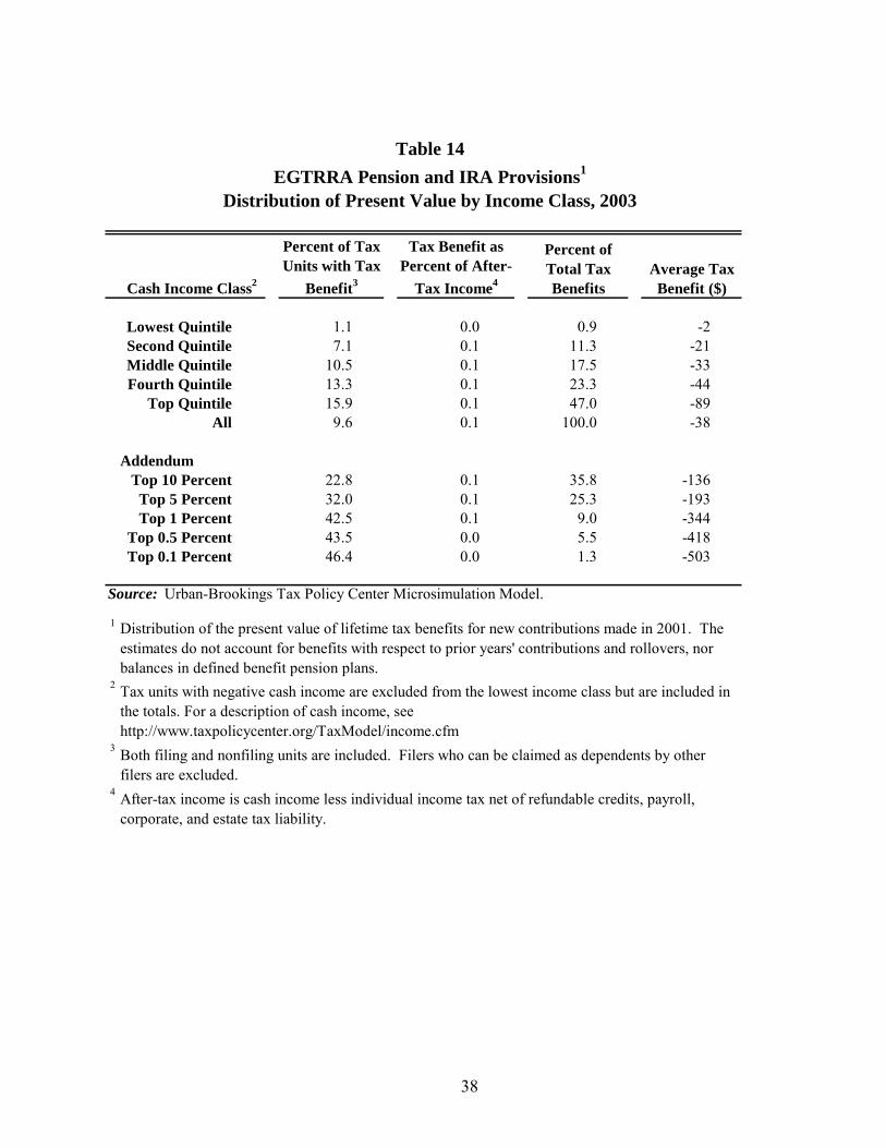
38

Lowest Quintile 1.1 0.0 0.9 -2Second Quintile 7.1 0.1 11.3 -21Middle Quintile 10.5 0.1 17.5 -33Fourth Quintile 13.3 0.1 23.3 -44

Top Quintile 15.9 0.1 47.0 -89All 9.6 0.1 100.0 -38

AddendumTop 10 Percent 22.8 0.1 35.8 -136

Top 5 Percent 32.0 0.1 25.3 -193Top 1 Percent 42.5 0.1 9.0 -344

Top 0.5 Percent 43.5 0.0 5.5 -418Top 0.1 Percent 46.4 0.0 1.3 -503

Source: Urban-Brookings Tax Policy Center Microsimulation Model.

1

Percent of Tax Units with Tax

Benefit3

Distribution of the present value of lifetime tax benefits for new contributions made in 2001. The estimates do not account for benefits with respect to prior years' contributions and rollovers, nor balances in defined benefit pension plans.

Both filing and nonfiling units are included. Filers who can be claimed as dependents by other filers are excluded.After-tax income is cash income less individual income tax net of refundable credits, payroll, corporate, and estate tax liability.

Table 14EGTRRA Pension and IRA Provisions1

Distribution of Present Value by Income Class, 2003

Cash Income Class2

Tax Benefit as Percent of After-

Tax Income4

Percent of Total Tax Benefits

Average Tax Benefit ($)

2

3

4

Tax units with negative cash income are excluded from the lowest income class but are included in the totals. For a description of cash income, see http://www.taxpolicycenter.org/TaxModel/income.cfm

39

y

Lowest Quintile 0.1 0.0 0.1 0 0.3 0.4Second Quintile 0.8 0.0 1.3 -3 1.9 5.4Middle Quintile 2.9 0.0 6.0 -14 1.9 9.3Fourth Quintile 6.0 0.1 17.5 -42 2.0 16.0

Top Quintile 16.3 0.1 75.1 -181 3.0 68.7All 5.2 0.1 100.0 -48 2.5 100.0

AddendumTop 10 Percent 23.4 0.1 56.0 -269 3.2 53.6

Top 5 Percent 32.8 0.1 41.0 -395 3.6 44.4Top 1 Percent 44.3 0.1 13.5 -649 5.2 33.3

Top 0.5 Percent 46.4 0.1 7.8 -751 5.5 27.1Top 0.1 Percent 49.5 0.0 1.7 -798 5.7 15.5

Source: Urban-Brookings Tax Policy Center Microsimulation Model.

1

2

3

4

Average Tax Benefit ($)Cash Income Class2

Percent of Tax Units with Tax

Benefit3

Tax Benefit as Percent of After-

Tax Income4

Percent of Total Tax Benefits

Tax units with negative cash income are excluded from the lowest income class but are included in the totals. For a description of cash income, see http://www.taxpolicycenter.org/TaxModel/income.cfmBoth filing and nonfiling units are included. Filers who can be claimed as dependents by other filers are excluded.After-tax income is cash income less individual income tax net of refundable credits, payroll, corporate, and estate tax liability.

Table 15EGTRRA Pension and IRA Provisions1

Distribution of Present Value by Income Class, 2010

Percent of Total Tax

Benefit

Addendum: all EGTRRA

Distribution of the present value of lifetime tax benefits for new contributions made in 2010. The estimates do not account for benefits with respect to prior years' contributions and rollovers, nor balances in defined benefit pension plans.

Percent Change in After-Tax

Income4

40

y

Lowest Quintile 1.4 0.0 1.1 -3Second Quintile 7.7 0.1 7.4 -21Middle Quintile 8.4 0.1 11.8 -34Fourth Quintile 8.2 0.1 18.3 -52

Top Quintile 16.4 0.1 61.3 -175All 8.4 0.1 100.0 -57

AddendumTop 10 Percent 23.4 0.1 45.1 -257

Top 5 Percent 32.8 0.1 32.3 -368Top 1 Percent 44.2 0.1 10.3 -588

Top 0.5 Percent 46.3 0.1 6.2 -710Top 0.1 Percent 49.4 0.0 1.4 -773

Source: Urban-Brookings Tax Policy Center Microsimulation Model.

1

2

3

4

Table 16

EGTRRA Pension and IRA Provisions, Including Extension of Saver's Credit1

Distribution of Present Value by Income Class, 2010

Cash Income Class2Tax Benefit as

Percent of After-Tax Income4

Percent of Total Tax Benefits

Average Tax Benefit ($)

Percent of Tax Units with Tax

Benefit3

Baseline is current law with pre-EGTRRA pension and IRA limits to contributions with the saver's credit extended at 2005 levels through 2010.

Both filing and nonfiling units are included. Filers who can be claimed as dependents by other filers are excluded.After-tax income is cash income less individual income tax net of refundable credits, payroll, corporate, and estate tax liability.

Tax units with negative cash income are excluded from the lowest income class but are included in the totals. For a description of cash income, see http://www.taxpolicycenter.org/TaxModel/income.cfm

41

Lowest Quintile 2 0 0 0 0 2Second Quintile 21 0 0 1 0 20Middle Quintile 33 1 0 4 0 28Fourth Quintile 44 7 0 11 1 25

Top Quintile 89 47 9 24 8 1All 38 11 2 8 2 15

AddendumTop 10 Percent 136 74 17 31 13 1

Top 5 Percent 193 106 34 31 22 0Top 1 Percent 344 139 156 24 25 0

Top 0.5 Percent 418 134 240 23 21 0Top 0.1 Percent 503 79 389 17 19 0

Source: Urban-Brookings Tax Policy Center Microsimulation Model.

1

2

Table 17Decomposition of EGTRRA DC and IRA Tax Benefits, 20031

In Dollars

Cash Income Class2

Average Total Tax Benefit3 Saver's Credit

Higher DC Contribution Limits

Catch-up Contributions

Employee Contribution

Employer Contribution

Tax units with negative cash income are excluded from the lowest income class but are included in the totals. For a description of cash income, see http://www.taxpolicycenter.org/TaxModel/income.cfm

Higher IRA Limits

Provisions are stacked against EGTRRA law (minus pension provisions) in the order shown. Changing the stacking order would change the dollar estimates significantly.

42

Lowest Quintile 0 0 0 0 0 3 3Second Quintile 3 0 0 3 0 21 18Middle Quintile 15 1 0 14 1 34 18Fourth Quintile 44 7 0 35 3 52 8

Top Quintile 174 79 13 67 15 175 1All 47 17 3 24 4 57 10

AddendumTop 10 Percent 257 134 27 73 24 257 0

Top 5 Percent 368 208 53 68 38 368 0Top 1 Percent 588 227 223 96 41 588 0

Top 0.5 Percent 710 218 330 122 41 710 0Top 0.1 Percent 773 149 450 134 40 773 0

Source: Urban-Brookings Tax Policy Center Microsimulation Model.

1

2

Saver's Credit

Average Total Tax

BenefitEmployee

ContributionEmployer

ContributionHigher IRA

Limits

Tax units with negative cash income are excluded from the lowest income class but are included in the totals. For a description of cash income, see http://www.taxpolicycenter.org/TaxModel/income.cfm

Provisions are stacked against EGTRRA law (minus pension provisions) in the order shown. Changing the stacking order would change the dollar estimates significantly.

Table 18Decomposition of EGTRRA DC and IRA Tax Benefits, 20101

In Dollars

Cash Income Class2

Average Total Tax

Benefit

Higher DC Contribution LimitsAssuming Saver's Credit

Extended

Catch-up Contributions

43

Less than 25 18,733 13.2 16.1 1.2 8.0 -30525-34 26,079 18.4 33.9 1.7 22.9 -62835-44 29,317 20.7 43.6 1.7 35.4 -86245-54 23,580 16.6 43.0 1.3 24.8 -75055-64 14,966 10.6 29.5 0.7 7.6 -364

? 65 29,101 20.5 3.4 0.1 1.3 -32All 141,777 100.0 28.3 1.1 100.0 -504

Source: Urban-Brookings Tax Policy Center Microsimulation Model.

1 Baseline is current law.2 Both filing and nonfiling units are included. Filers who can be claimed as dependents by other filers are excluded.3 After-tax income is cash income less individual income tax net of refundable credits, payroll, corporate, and estate tax liability.

Percent with Tax Benefit

Table 19Tax Benefits of All Defined Contribution Plans1

Present Value of Tax Benefits by Age of Household Head, 2003

Age Bracket

Tax Units2Percent Change

in After-Tax Income3

Percent of Total Income Tax Benefit

Average Tax Benefit ($)

Number (thousands)

Percent of Total

44

Less than 25 20,822 13.4 17.3 1.3 7.9 -40025-34 28,384 18.3 35.6 1.8 22.9 -85335-44 31,290 20.1 44.6 1.8 34.8 -1,17245-54 25,559 16.4 44.4 1.4 25.0 -1,03355-64 16,421 10.6 31.4 0.8 7.9 -509

? 65 32,958 21.2 3.5 0.1 1.5 -47All 155,433 100.0 29.1 1.2 100.0 -679

Source: Urban-Brookings Tax Policy Center Microsimulation Model.

1 Baseline is current law.2

Both filing and nonfiling units are included. Filers who can be claimed as dependents by other filers are excluded.3 After-tax income is cash income less individual income tax net of refundable credits, payroll, corporate, and estate tax liability.

Percent with Tax Benefit

Table 20Tax Benefits of All Defined Contribution Plans1

Present Value of Tax Benefits by Age of Household Head, 2010

Age Bracket

Tax Units2Percent Change

in After-Tax Income3

Percent of Total Income Tax Benefit

Average Tax Benefit ($)

Number (thousands)

Percent of Total

45

Less than 25 20,822 13.4 17.3 1.3 8.0 -41025-34 28,384 18.3 35.6 1.8 22.9 -86535-44 31,290 20.1 44.6 1.8 34.6 -1,18445-54 25,559 16.4 44.4 1.4 25.0 -1,04455-64 16,421 10.6 31.4 0.8 8.0 -520

? 65 32,958 21.2 3.5 0.1 1.5 -49All 155,433 100.0 29.2 1.2 100.0 -688

Source: Urban-Brookings Tax Policy Center Microsimulation Model.

1 Baseline is current law.2 Both filing and nonfiling units are included. Filers who can be claimed as dependents by other filers are excluded.3 After-tax income is cash income less individual income tax net of refundable credits, payroll, corporate, and estate tax liability.

Percent with Tax Benefit

Table 21Tax Benefits of All Defined Contribution Plans, Assuming Extension of the Saver's Credit1

Present Value of Tax Benefits by Age of Household Head, 2010

Age Bracket

Tax Units2 Percent Change in After-Tax

Income3

Percent of Total Income Tax Benefit

Average Tax Benefit ($)

Number (thousands)

Percent of Total

46

Lowest Quintile 0.0 0.0 0.1 0Second Quintile 0.6 0.0 2.1 -2Middle Quintile 1.7 0.0 7.5 -7Fourth Quintile 3.1 0.0 18.8 -18

Top Quintile 9.6 0.1 71.5 -69All 3.0 0.0 100.0 -19

AddendumTop 10 Percent 14.6 0.1 54.4 -104

Top 5 Percent 22.2 0.1 38.1 -146Top 1 Percent 34.8 0.0 10.7 -205

Top 0.5 Percent 36.2 0.0 4.7 -182Top 0.1 Percent 39.1 0.0 0.7 -142

Source: Urban-Brookings Tax Policy Center Microsimulation Model.

1Baseline is current law.

2

3

4

Table 22Accelerate EGTRRA DC and IRA Contribution Limit Increases1

Present Value of Income Tax Change by Income Class, 2004

Cash Income Class2

Percent Change in After-Tax

Income4

Percent of Total Income Tax Benefit

Average Tax Benefit ($)

Both filing and nonfiling units are included. Filers who can be claimed as dependents by other filers are excluded.After-tax income is cash income less individual income tax net of refundable credits, payroll, corporate, and estate tax liability.

Percent of Tax Units with Tax

Benefit3

Tax units with negative cash income are excluded from the lowest income class but are included in the totals. For a description of cash income, see http://www.taxpolicycenter.org/TaxModel/income.cfm

47

y

Lowest Quintile 4.8 0.2 14.6 -17Second Quintile 8.6 0.3 38.2 -44Middle Quintile 7.0 0.1 34.3 -39Fourth Quintile 2.5 0.0 8.9 -10

Top Quintile 0.3 0.0 2.6 -3All 4.6 0.1 100.0 -23

AddendumTop 10 Percent 0.2 0.0 1.3 -3

Top 5 Percent 0.1 0.0 0.4 -2Top 1 Percent 0.1 0.0 0.1 -1

Top 0.5 Percent 0.1 0.0 0.0 -1Top 0.1 Percent 0.1 0.0 0.0 -2

Source: Urban-Brookings Tax Policy Center Microsimulation Model.

1 Baseline is current law.

2

3

4

Table 23Make Saver's Credit Refundable1

Distribution of Income Tax Change by Income Class, 2004

Cash Income Class2

Percent Change in After-Tax

Income4

Percent of Total Income Tax Benefit

Average Tax Benefit ($)

Both filing and nonfiling units are included. Filers who can be claimed as dependents by other filers are excluded.After-tax income is cash income less individual income tax net of refundable credits, payroll, corporate, and estate tax liability.

Percent of Tax Units with Tax

Benefit3

Tax units with negative cash income are excluded from the lowest income class but are included in the totals. For a description of cash income, see http://www.taxpolicycenter.org/TaxModel/income.cfm

48

IX. Figures

49 IX. Figures

Figure 1Distribution of EGTRRA Pension Provisions

Compared with all EGTRRA Income Tax Provisions, 2010

0

10

20

30

40

50

60

70

80

90

100

0 10 20 30 40 50 60 70 80 90 100

Percent of Filing Units

Perc

ent o

f Tax

Cut

s

All EGTRRA Pension Provisions Pension plus Savers Credit

Source: Tax Policy Center Microsimulation Model.

50

Figure 2. Decomposition of EGTRRA Pension Tax Benefits, 2003

29%

5%

21%5%

40% Employee ContributionEmployer ContributionHigher IRA LimitsCatch-up ContributionsSaver's Credit

Figure 3. Decomposition of EGTRRA Pension Tax Benefits Assuming Savers Credit Extended, 2010

30%

5%

42%

6%

17%

Employee ContributionEmployer ContributionHigher IRA LimitsCatch-up ContributionsSaver's Credit

51

X. Appendix: Modeling Savings Tax Incentives

To model the effects of EGTRRA on retirement savings and the distribution of tax burdens, we measure the following for each adult head and spouse in a tax unit:

• Coverage by DB pension plan • Coverage by DC pension plan • Conditional on coverage by DC plan,

o Amount of employer contribution, if any o Amount of elective deferral (employee contribution), if any

• Participation in an IRA, type of IRA, and contribution conditional on participation To do this, we combine data from four sources. The 1999 Public Use File (PUF)

produced by the Statistics on Income Division of the IRS is the input data set for the Tax Policy Center’s individual income tax model, used as the basis of our estimates of the revenue consequences of tax changes and their effects on the distribution of tax burdens. These data are excellent for calculating income tax liability and marginal tax rates, but they exclude most information about pensions and IRAs as well as important demographic information such as age.

We map pension and IRA information onto the PUF from two other data sources—the

2001 Survey of Consumer Finances (SCF), produced by the Federal Reserve Board, and the 1996 Survey of Income and Program Participation (SIPP), produced by the Census Bureau. The SCF has the best available data on pension participation but does not report the amount of IRA contributions. (Total IRA contributions are reported on the PUF, but there is no information about the eligibility, dependent on income and pension participation, of those who choose not to contribute.) Wave 7 of the 1996 SIPP, collected between April and July 1998, reports IRA participation and contribution levels for head of household and spouse in 1997.

In addition, we match demographic information from the 2000 Current Population

Survey onto the PUF using statistical matching techniques. Doing so provides measures of earnings for head and spouse, their ages, the ages of their children, and so on.

A. Pension Contribution and Coverage

1. Estimation

We impute DC and DB coverage and contribution levels in two steps: (1) Does the item exist for the household? (2) For those who have nonzero amounts of the item, what is the level? We use the probit maximum likelihood estimator to estimate the likelihood of having each item, and censored regression to estimate the amount. The procedure is similar to the Heckman two-step estimator, but without the Mills ratio correction in the second stage. This approach may yield biased coefficient estimates in the second stage, but that is not relevant here because we have no interest in the point estimates. All we care about is producing the best fit, conditional on the explanatory variables.

52

We estimate the probability of having each item using probit maximum likelihood. Under

the probit model, the item is observed if and only if X1β1 + ε1 > 0, where ε1 is assumed to be a standard normal random variable with mean 0 and variance 1. Conditional on reporting any amount of a particular item, we estimate the amount as a function of a similar set of variables. Since contributions to pension plans are limited by law to certain dollar maximums, we must estimate the second stage using censored regression techniques. The model is identical to that for the least squares estimator, except that it assumes normality of the error term and accounts for the fact that there is a statutory upper bound on each item.24

For each contribution item (excluding defined benefit pension contributions, which are

not available), we estimate an equation of the form ln(y*) = X2β2 + ε2, where y* is the desired contribution (before application of statutory limits), and ε2 is assumed to be normal with mean 0 and variance σ2. The latent variable, y*, is not observed. Instead, we observe y, defined as y* when y* < L, otherwise L, where L is the statutory limit on contributions. The upper limits for the censored regression are based on the law in effect in 2000. The maximum elective contribution to a 401(k) was limited to the lesser of $10,500 or 25 percent of earnings, and the maximum total qualifying contribution (including both employer and employee share) was limited to $30,000.25,26

The list of exogenous variables for each probit and censored regression is designed to be

an exhaustive set of relevant variables that exist on both the SCF and the PUF. These variables include number of dependents, age (included as 10-year bracket dummies), income (as defined for purposes of the SCF), and the following components of income: income from a farm or business, tax-exempt interest income, taxable interest income, rental income from schedule E, pension income, taxable dividends, and realized capital gains (all defined as the natural logarithm of the income item plus one). We also include dummies for zero values of each income item; dummies for negative overall income, negative income from a business or farm, and negative capital income; as well as interactions between the negative income dummies and the appropriate negative income amount (defined as the natural logarithm of the absolute value of the income item plus one). In addition, we include dummies for whether the individual itemizes deductions on his or her federal tax return and dummies for whether certain federal tax schedules are filed (C for business income, E for rental income, and F for farm income). The list of explanatory variables is identical for each equation, except for the employer contribution

24 The statement Y = Xβ + ε < L implies that ε < L - Xβ. The truncation thus introduces a spurious correlation

between the error term and the vector of explanatory variables, X. Under this circumstance, least squares estimates are biased and inefficient. Put more simply, the truncation provides information about the distribution of the error term. Using that information makes the estimates better.

25 In some cases, earnings reported separately for each spouse were inconsistent with total household earnings.

In that case, total earnings were apportioned between the spouses in proportion to their reported separate earnings. If positive household earnings were reported but the individuals did not report earnings separately, we attributed the total amount to the head of household.

26 Some employees reported contributing more than the limit. We assumed that any excess contributions were

made to a nonqualifying pension plan.

53

probit and level equations. Those equations include the log of employee contributions as an explanatory variable, under the logic that employer contributions are often matching—the more the employee contributes, the larger the employer match, up to some limit.

Equations are estimated separately for head of household and spouse, but based on

household level values for the explanatory variables with the exception of age and earnings.27 It is not appropriate in the SCF to simply run regressions or probits on the entire data set

because of its approach to missing variables. The SCF imputes missing values for a number of fields. To reflect the variance introduced by that process, the SCF database includes five replicates of each observation. Missing values are drawn randomly for each replicate from the estimated probability distribution of the imputed value, whereas nonmissing values are simply repeated. We estimate coefficients by computing each estimate separately for each sample replicate and then averaging the coefficient estimates.28

2. Imputation

We impute values for the pension items on the basis of the estimation results. We then calibrate the results to match SCF aggregates for each item.

Imputation on the individual income tax model is done in two steps: 1) Simulate whether the taxpayer has the item:

• For consistency, pension contributions are attributed only to tax returns that are not shown to be ineligible by virtue of their IRA contributions. (Tax returns include data on contributions to traditional IRAs. Since taxpayers above certain AGI thresholds may not make contributions to IRAs if their employers offer a pension, any in those categories who report IRA contributions must not participate in an employer plan.)

• For each item, using the estimated coefficients from the probit estimation and values of

explanatory variables in the tax model database, calculate Xb1 (where b1 refers to the probit estimate for β1).

27 The SCF is a household-based survey that records only total income and wealth items for all individuals in

the "primary economic unit" (PEU); it does not attribute shares of those amounts to individuals within the PEU. This introduces a slight complication for PEUs that consist of two unmarried individuals living together (with or without other financially interdependent members of the PEU). These individuals will show up in the income tax file as two single tax returns but will show up in the SCF as one unit. We assume that an unmarried couple living together with shared finances behaves like a married couple and thus include them in the married category when running the regressions. The results do not change significantly if these individuals are dropped from the analysis.

28 We also correct the standard errors using the procedure supplied by the Federal Reserve Board, but it is not a

particularly important adjustment, given that we are not interested in the parameter estimates. The corrected estimates and standard errors from that procedure, as well as a measure of goodness-of-fit from the first replicate, are available upon request.

54

• Calculate the threshold probability, z = Φ-1(X1b1), where Φ is the cumulative standard normal probability distribution.

• Draw a uniform random number, p, between 0 and 1.

• If z < p, assign a nonzero value for the item.29

2) Estimate the amount of each item for taxpayers with z < p: • Using the estimated coefficients from the level equation (b2) and values for explanatory

variables in the PUF, calculate Xb2. • Calculate the desired value for the item, y. In the limit, E(y*) = exp(Xb2+s2/2), where s is

the estimated standard error for the level regression. However, in finite samples, exp(Xb2+s2/2) can be a biased estimator, and the biases can be large if the errors are in fact nonnormal. We follow Duan (1983) and instead use a robust empirical “smearing adjustment” to match the sample means of predicted values with the sample mean of the actual SCF data. The adjustment basically amounts to multiplying exp(Xb2) by a constant chosen to align the sample means.

• The explanatory variables for each equation are the same, except that the log of employee

contributions is added to the equations explaining employer participation and contribution levels (under the logic that many employer contributions are designed as matching, which implies that they are conditional on contributions by the employee).

3. Calculating Gross Wages

After the imputation process is complete, we calculate gross wages by adding employer and employee contributions to DC pension plans to reported taxable wages and salaries. The advantage of this method is that it is invariant with respect to changes in tax incentives. Assuming that employer contributions to pension plans and other fringe benefits are paid out of wages, pension tax incentives can and do affect wages reported on tax returns, but not gross wages. By the same logic, we subtract the employer’s portion of additional payroll taxes due on the additional cash compensation from gross wages. Thus, the relationship between taxable wages and gross wages is as follows:

w1 (1+τp) = w0 (1+τp) + f0 ,

29Without adjustment, this process can produce too many or too few individuals with pension contributions on the PUF data set. We force the numbers to match published totals by shifting the threshold probabilities by a constant (up or down), so that the simulated number of contributors matches the estimates on the SCF.

55

where w1 is gross wages, w0 is taxable wages, τp is the combined Social Security and Medicare payroll tax rate, and f0 is the value of fringe benefits (including pension benefits) imputed in the baseline. Gross wages are, therefore,

w1 = w0 + f0 / (1+τp). That is, gross wages are not increased by the full amount of the fringe benefit, because paying additional cash wages entails an additional cost to the employer in payroll taxes. By similar logic, under the policy simulations, taxable wages, w′, equal

w′ = w1 - f′ / (1+τp).

B. IRA Participation and Contributions

IRAs raise special issues for three reasons. First, IRA contributions are not reported on the SCF. We solve this problem by basing our imputation on the 1996 SIPP. Second, no questions were asked about Roth IRAs in the SIPP (the program was first enacted in 1997), and no cross-section data are available on Roth IRA contributions. Third, 1997 legislation phased in substantial increases to the income limits for contributions to traditional IRAs—not fully effective until 2007. This last point means that baseline contributions can be significantly greater in later years than the observed values for taxpayers who are at the limit in 1997.

To calculate the baseline distribution of IRA participation and contribution levels, we use

a method similar to the one described above, modified to use information in the PUF about contributions to traditional IRAs. A taxpayer who contributes to a tax-deductible IRA, as indicated in the PUF in 1999, is assumed to contribute to such an account in later years. Moreover, taxpayers who contribute the limit are assumed to contribute more when IRA limits increase. For everyone else, participation depends on the results of probit equations estimated on the 1997 SIPP data (as described above for 401(k) plans), and the desired level of contribution depends on the predictions of a censored regression equation also estimated on the SIPP.

To simplify, we assume that, when eligible for both types of IRA, these other taxpayers

all contribute to Roth IRAs, even if they become eligible for traditional IRAs as the limits increase. Because the present value of Roth and traditional IRAs is equivalent for an equal after-tax contribution (as discussed below), this assumption does not affect the distribution of tax benefits from IRAs overall, but it may cause an overestimate of the share of contributions to Roth IRAs, especially for those with higher incomes. On the other hand, it is likely (although not provable right now), that more higher income people will be shifting from traditional IRAs to Roth IRAs over time as awareness of the new (in 1997) program grows. In addition, those who would like to make an after-tax contribution of more than L (1-τ), where L is the contribution limit and τ is the marginal income tax rate, can do so only through a Roth IRA. So, on balance, this simplifying assumption seems reasonable.

56

As noted, we assume that those who contribute to traditional IRAs in 1999 also contribute to traditional IRAs in later years. We adjust the contribution amount to reflect the higher contribution limits and increases in income in later years. For those who contribute the limit to an IRA in 1999, their desired contribution is at least the limit amount. We calculate the desired contribution on the basis of the estimates from the censored regression equation. Suppose the limit in 1999 was L, the actual contribution was I, the vector of explanatory variables is X, the coefficient vector from the censored regression is denoted as β3, and the error as ε3, a random variable with mean 0 and variance σ3. Let ln(I*) = X β3 + ε3 represent the desired contribution. The dependent variable is upward censored at ln(L), so the observed variable is ln(I) = ln(I*) when I* < L and ln(I) = ln(L) otherwise. For limit contributors, the expectation of I* is

3 3

3 3( * | ) ( | ln( ) ).XE I I L E e L Xβ ε ε β+≥ = ≥ − It may be shown that

2

3 3

23 3

3/ 2

3

3

ln1( * | ) .

ln1

X

L X

E I I L eL X

β σ

β σσ

βσ

+

⎛ ⎞− −−Φ⎜ ⎟

⎝ ⎠≥ =⎛ ⎞−

−Φ⎜ ⎟⎝ ⎠

We calculate a consistent estimator for this expected value using the estimates for the coefficient vector and standard error generated by the censored regression equation. (Basically, this procedure guarantees that predicted contributions are at least as great as the 1999 limit, which means that these people will contribute more when the limit increases.)

For all other taxpayers who are eligible for Roth IRAs (including those eligible for

traditional IRAs who do not contribute to such an account), we use the estimated probit equation and censored regression estimates to predict whether they contribute to a Roth IRA and the amount of desired pretax contribution (since the traditional IRAs were all made on a pretax basis). The procedure is identical to that outlined for 401(k) participation and contributions, except for two modifications. First, the contribution is converted from a pretax to an after-tax contribution based on the taxpayer’s marginal tax rate (subject to the applicable Roth IRA limit). Then, the estimates for participation and contribution levels are calibrated to match in 2000 estimates published by the IRS in Sailer and Nutter (forthcoming).

C. Modeling the Saver’s Credit and Alternatives

The saver’s credit is a tax credit equal to a share of employee contributions to DC pensions and IRAs. We model this credit simply as a reduction in tax based on the credit formula. Following standard distributional analysis conventions, no behavioral response is assumed—that is, we do not assume that saving increases when people have access to the credit. Thus, the credit calculation follows directly from our estimates of IRA and retirement plan contributions.

57

For some scenarios, we assume that the credit is refundable. That means that tax filers get the full benefit of the credit even if it exceeds their income tax liability—even if they do not owe income tax at all.

D. Simulating Alternative Policies

We simulate alternative policies—most notably, higher contribution limits and changes in income eligibility rules—using an analogous procedure. It is assumed that people who are eligible to contribute in the baseline but do not contribute will not decide to contribute if their contribution limit increases (this assumption could be wrong if there are transaction costs), but those who do contribute in the baseline and are at the limit will increase their contribution if the limit increases up to their desired contribution or the limit, whichever is lower. Changes in income limits for IRA contributions could also increase the number of contributors, as some newly eligible people would contribute, depending on the prediction of the probit participation equation, as discussed above.30

E. Calculating the Present Value of Tax Benefits from IRAs and Pensions

We calculate the value of pension and IRA tax benefits by comparing the taxation to a taxable account holding a similar level of after-tax contributions. Consider a contribution of $1,000 to a traditional (deductible) IRA. The cost of that contribution is $1,000(1-τ). Call that amount V0. Assuming that, alternatively, that money would be contributed to a taxable account paying a rate of return r and taxed at constant rate, τ, the account would be worth

t

t 0V = V (1+r(1- ))τ

after t years, where t = 1,…,N, and N is the year at which withdrawals start (at the end of the year). Assuming discounting at rate r, the present value of taxes during the N-year accumulation phase is

01 (1 )1

1

N

NrPV V

rτ⎡ ⎤+ −⎛ ⎞= −⎢ ⎥⎜ ⎟+⎝ ⎠⎢ ⎥⎣ ⎦

.

If the money is withdrawn in a lump sum at the end of year N, this would be the present

value of the tax benefits. We follow Cronin (1999) in assuming that the contribution period is until age 65 and then the money is withdrawn in equal portions starting at age 66 until the end of the life expectancy. Withdrawals are assumed to occur at the end of the year, after interest has accrued.

If life expectancy at age 65 is 65 + T, then the annual withdrawal, A, will solve the

following equation

30 This feature would be used to model recent proposals to eliminate income limits entirely for eligibility for

contributions to Roth IRAs.

58

1 (1 )1 (1 (1 ))(1 )

TN

rV A rr

τττ

− + −⎡ ⎤= − + −⎣ ⎦ −,

where VN is the value of the taxable account at age 65 (at the end of the year).

It may be shown that the value of the taxable account during the retirement period is

1

11

jj

N j NV V A γγγ

−

+ −

⎡ ⎤−= −⎢ ⎥−⎣ ⎦

,

where 1 (1 ).rγ τ≡ + −

Tax in period N+j is

11

11

jj

N j NV A rγθ γ τγ

−−

+ −

⎡ ⎤−= −⎢ ⎥−⎣ ⎦

.

Thus, the present value of the taxes saved is

1

.(1 )

TN j

N N jj

PV PVr

θ ++

=

= ++∑

1. Assumptions for Calculations

For a deductible IRA or 401(k) contribution, V0 is the after-tax cost of the contribution (i.e., multiplied by 1-τ). For a Roth IRA or 401(k), V0 is the amount of the contribution. Thus, for someone in the 25 percent tax bracket, a $2,000 contribution to a traditional IRA would be analogous to a $1,500 contribution to a taxable account (V0 = 1,500). A $2,000 contribution to a Roth IRA would be analogous to a $2,000 contribution to the taxable account (V0 = 2000).

For this calculation, τ should be the marginal tax rate on earnings. For simplicity, assume

that the tax rate on savings outside of retirement accounts is also τ (as assumed in the calculation above). In fact, the effective rate might be lower if, for example, the account pays returns in the form of capital gains or dividends. This assumption will thus tend to overstate the value of the retirement tax incentives.

However, we will also make a conservative assumption about the rate of return on the

taxable account. We assume that r is 6 percent—3 percent inflation plus 3 percent real growth—as assumed in the 2003 Social Security Administration trustees report. To the extent that the taxable account would be invested in stocks or commercial bonds, there would be a risk premium that would raise the expected return. Thus, this assumption will tend to offset the bias from assuming full taxation of returns.

59

XI. Glossary

Actuarial balance: A situation in which the present value of receipts equals the present value of expenditures. For example, if Social Security were in 75-year actuarial balance, it would be able to pay all of its obligations out of receipts plus the trust fund (including interest) for the next 75 years. Adjusted gross income (AGI): The amount of income counted to determine a filing unit’s tax liability. Certain types of income received or payments made (e.g., alimony paid, IRA deductions, moving expenses) are excluded from AGI. Administrative burden: The costs of complying with the law. A company’s administrative burden adds to the cost of producing goods or services. Alternative minimum tax (AMT): An alternative income tax that was designed to ensure that high-income filers who use tax preferences to substantially reduce or eliminate their tax liability under the regular income tax pay some minimum amount. Since it is not indexed for inflation, the AMT will increasingly affect middle-income families. Annuity: An investment on which a person receives fixed payments for a lifetime or a specified number of years. Beneficiary: The designated recipient of certain benefits. Capital: The general term used to describe any money or assets put to economic use. Depending on the asset, capital takes different forms. Human capital refers to the knowledge and skills that workers acquire through education, training, and experience. Physical capital describes fixed assets, such as buildings, machinery, raw materials, and products. Current Population Survey (CPS): A monthly survey of about 50,000 households conducted by the Bureau of the Census for the Bureau of Labor Statistics. The sample is selected to represent the civilian noninstitutionalized population. Estimates obtained from the CPS include employment, unemployment, earnings, hours of work, and other indicators, and are available by a variety of demographic characteristics, including age, sex, race, marital status, educational attainment, occupation, industry, and class of worker. Supplemental questions are often added to the regular CPS questionnaire on topics such as retirement or health to yield additional information. Deduction: A reduction in taxable income for certain expenses. Some deductions, such as those for contributions to an individual retirement account, reduce adjusted gross income. Most deductions, such as those for home mortgage interest and state and local taxes, are available only to those who itemize deductions. Deductions cannot reduce taxable income below zero.

60

Deferred compensation: Compensation paid by an employer after the income is earned, often intended to finance retirement. Employees do not pay taxes on qualified deferred compensation until the money is distributed at a later date. As a result, the money is able to grow tax-free.

Defined benefit retirement plan: A retirement plan that guarantees a specified retirement payment at a certain age and after a specified period of service.

Defined contribution retirement plan: A retirement program in which each employee has an individual account that accumulates employee contributions and/or employer contributions plus investment returns on account balances.

Distribution: How a proposal or policy affects the distribution of tax burdens by income, demographics, or other characteristics. Estate and gift tax: A tax levied on the value of assets held at the time of death above a certain threshold. The threshold is $1.5 million in 2004. Deductions are allowed for transfers to a spouse, gifts to charity, expenses, and state taxes levied on estates and inheritances.31 Gifts--transfers between individuals where less than full value is received in return--before death in excess of $11,000 (in 2004) are also subject to a gift tax, which is deductible against the estate tax at time of death. Gross domestic product (GDP): The total value of all goods and services produced by a nation’s residents and property during some specified period of time. GDP is often used as a benchmark for assessing levels of expenditures. Indexing: Adjustment to dollar amounts to account for inflation. For example, the standard deduction, personal exemptions, and tax rate thresholds are increased every year by an inflation index. The measure of inflation most often used is the Consumer Price Index. Individual retirement accounts (IRAs): Retirement accounts funded by individuals through their own contributions or by rolling over benefits earned under an employee-sponsored plan. Contributions to traditional IRAs are deductible and investment earnings are untaxed, but withdrawals are taxable. Contributions to so-called Roth IRAs are not deductible, but earnings and withdrawals are tax-free. Liability (tax): The amount of total taxes owed after tax credits have been applied. Marginal tax rate: The tax rate that would have to be paid on an additional dollar of income. Marginal tax rates affect individuals' incentives to work, save, and shelter income from tax. National saving: The sum of private saving and public saving. Nondiscrimination rules: Provisions governing the levels of benefits that employers can provide to highly paid employees, as opposed to rank-and-file employees.

31 In 2001, a credit was allowed for most state taxes, but EGTRRA phased the credit out between 2002 and 2004.

61

Present value: The current equivalent value of a future stream of payments (either income or cost). The present value of a future stream of payments may be thought of as the lump-sum amount that one would require in place of the payment stream. This lump-sum amount, if invested today, together with interest earnings, should be enough to meet each of the payments as they fell due with zero remaining in the account after the last payment. Private saving: The excess of income over expenditures (including taxes) for all nongovernment entities—citizens, businesses, and so on. Progressivity: The extent to which tax burdens, measured as a percentage of income, increase with income. A progressive change in the tax code increases the after-tax income of lower earners relative to that of higher-earning individuals or households. For the converse, see Regressivity. Public Use File (PUF): A database of income tax information compiled by the Statistics on Income Division of the Internal Revenue Service, available for public use. Public saving: The excess of receipts over expenditures for all government entities. A surplus represents positive public saving, whereas a deficit represents public borrowing (or “dissaving”). Refundable: Refundability is a feature of certain tax credits that permits filers with low or no tax liability to receive the full value of the benefit by having the excess of tax liability paid back to the filer in the form of a rebate. For example, suppose a filer is eligible for a $400 credit and has only $100 in tax liability. If the credit is refundable, the filer will receive a rebate for the $300 difference. Regressivity: The extent to which tax burdens, measured as percentage of income, decrease as income increases. A regressive change in the tax code increases the after-tax income of higher earners more relative to that of lower-earning individuals or households. For the converse, see Progressivity. Retirement Savings Accounts: The President’s 2005 Budget proposed to create Retirement Savings Accounts to which individuals of any age could save up to $5,000 for their retirement in a tax-free account. Although contributions would not be tax-deductible, qualified distributions—those made after the account holder turns 58 or when the holder dies or becomes disabled—would be tax-free. Risk (economic, investment): The chance of things not turning out as expected. In general, economists assume that exposure to higher levels of risk requires higher expected returns. Sunsets: Tax provisions slated in law to expire on a certain date unless legislation is passed extending them.

62

Survey of Consumer Finances (SCF): A stratified sample of approximately 4,500 households conducted by the Board of Governors of the Federal Reserve. The survey is conducted triennially and contains detailed data on wealth and savings. Survey of Income and Program Participation (SIPP): A series of nationally representative data panels conducted by the U.S. Census Bureau that compile detailed information on income, labor force participation, and program participation on a monthly basis. Households are interviewed every four months; each of these interviews is called a "wave." The most recent survey began in 2001 and had nine waves (lasting three years), but earlier samples ranged in duration from two and a half to four years. Sample sizes have ranged from 14,000 to 36,700 households. Waves after the first may include so-called topical modules with additional questions about specific subjects, such as pensions or health. The survey collects data on taxes, assets, liabilities, and participation in government transfer programs. SIPP data help the government estimate costs and coverage for future programs. Tax preferences: Special provisions in the tax code, such as exclusions, deductions, credits, or preferential rates, that reduce tax liability and are not required to properly measure income. Vesting: The specific process by which employees accrue rights to employer contributions that are made to the employee's retirement account.