The Effects of Public Spending Externalities Publications Research/wp201210.… · Assessing the...

working papers

10 | 2012

April 2012

The analyses, opinions and fi ndings of these papers represent the views of the authors, they are not necessarily

those of the Banco de Portugal or the Eurosystem

THE EFFECTS OF PUBLIC SPENDING EXTERNALITIES

Valerio Ercolani

João Valle e Azevedo

Please address correspondence toValerio Ercolani

Banco de Portugal, Economics and Research Department Av. Almirante Reis 71, 1150-012 Lisboa, Portugal;

Tel.: 351 21 313 0065, email: [email protected]

BANCO DE PORTUGAL

Av. Almirante Reis, 71

1150-012 Lisboa

www.bportugal.pt

Edition

Economics and Research Department

Pre-press and Distribution

Administrative Services Department

Documentation, Editing and Museum Division

Editing and Publishing Unit

Printing

Administrative Services Department

Logistics Division

Lisbon, April 2012

Number of copies

85

ISBN 978-989-678-130-9

ISSN 0870-0117 (print)

ISSN 2182-0422 (online)

Legal Deposit no. 3664/83

The Effects of Public Spending Externalities

Valerio Ercolani∗

Bank of Portugal

Joao Valle e Azevedo

Bank of Portugal

Nova School of Business and Economics

March 26, 2012

Abstract

We take to the data an RBC model with two salient features. First, we allow government consumption

to directly affect the marginal utility of consumption. Second, we allow public capital to affect the

productivity of private factors. On the one hand, private and government consumption are estimated to

be substitute goods. As a consequence, the estimated response of private consumption to a government

consumption shock is negative, as in models with separable government consumption, but such response

is much stronger. Further, substitutability makes labor supply to react less, so the estimated output

multiplier is lower than in models with separabilities, peaking - on impact - at 0.39. On the other

hand, non-defense public investment enhances mildly or negligibly, depending on the specification, the

productivity of private factors. In those specifications where non-defense public investment is found to

be productive, a non-defense investment shock generates the following estimated responses (after several

quarters): a positive reaction for private consumption, Tobin’s q, private investment and real wages.

Unlike models with unproductive government investment, the estimated output multiplier builds up over

time, starting well below one on impact, then reaching 0.93 after three years and 1.44 after six.

JEL classification: E32, E62

Keywords: Public Spending Externalities, Fiscal Multipliers,

Government Consumption, Government Investment, Bayesian Estimation.

∗Corresponding author: E-mail: [email protected]. We thank Isabel Correia, Carlo Favero, Ricardo Felix, NikolayIskrev, Leonardo Melosi, Caterina Mendicino, Tommaso Monacelli, Nicola Pavoni, Pedro Teles and Roberto Perotti for usefulcomments. Earlier drafts of the paper have also benefited from discussions with Javier Perez, Gianni Amisano, and Frank Smets.Remaining errors are solely ours.

1

1 Introduction

Assessing the mechanisms through which government spending affects the private sector occupies a large

portion of the macroeconomic literature (see Ramey 2011a for a review of the leading theories on the effects

of government spending). We focus on channels resulting from “externalities” produced by government

spending and, importantly, we aim at understanding and measuring the effects of such externalities. By

externality we mean that government consumption can affect households’ marginal utility of consumption

and, therefore, the level of consumption itself. This occurs if some items of government spending act as

substitutes or complements for private consumption. For example, public health care can reduce the need

for private health services, or, public education services can reduce the need for private tutors and schools

but, on the other hand, increase the demand for textbooks or personal computers. These potential relations

between private consumption and different items of public spending make government consumption, on the

aggregate, to be either substitute or complement for private consumption. Thus, omitting a priori the po-

tential channel of substitutability/complementarity can produce a bias in the estimates of the response of

private consumption to a government consumption shock. Also, government investment can create exter-

nalities for the private sector. Specifically, public capital can act as a shifter of the productivity of private

factors, such that an increase in public investment has the potential to create a positive wealth effect, affect-

ing the dynamics of private investment as well as of consumption. For example, an efficient system of public

highways built in place of an old route can enhance the productivity of private factors for firms operating

in that area (e.g. by fostering within-country trade). Again, omitting this role for government investment

can bias estimates of the effects of such investment.

The standard hypothesis of the bulk of RBC (e.g. Baxter and King 1993) and new Keynesian models

(e.g. Smets and Wouters 2007) is that private and government consumption are separable in preferences or

that government consumption is a pure waste of resources.1 Moreover, even public capital is often omitted

since it is assumed to be “unproductive”. Within these models, the so called negative wealth effect is the

main driver of spending shocks. If government spending increases, then the present discounted value of taxes

to be paid by households also increases and so permanent income is lower. The well known consequence

of this effect is the negative correlation between public spending and private consumption conditional on

government spending shocks.2 The negative wealth effect positively impacts on labor supply which, in turn,

1However, it is worth noting that already Bailey (1971) and Barro (1981) identified the substitutability relation betweenprivate and government consumption as a possible mechanism through which public spending exerts its effects on privatedecisions.

2Notable exceptions can be found in the literature. For example, Galı, Lopez-Salido and Valles (2007) introduce a marketimperfection in a new Keynesian model, namely, a share of the population cannot borrow or lend. Because of this, aggregateconsumption can increase after a government spending shock. Following a different route, Linnemann (2006) builds a neoclassical

2

generates an increase in output and a decrease in real wages.3 Finally, private investment usually falls in

response to a (temporary) government spending shock.

Against this background, it is clear that the externalities we explore have the potential to reverse the

usual sign of the model variables’ reactions to government spending shocks or, even if the sign is correct, to

assess the likely bias of that response. For example, evidence of substitutability (complementarity) between

private and government consumption leads, ceteris paribus, to a negative (positive) response of private

consumption to a government consumption shock. Also, allowing for the possibility that public capital

affects the productivity of private factors may induce government investment shocks to create positive

wealth effects in the economy, hence generating positive reactions for private consumption, investment, and

real wages, ceteris paribus. Last but not least, if one is interested on the magnitude of the output effect of

fiscal stimulus, the responses obtained in Uhlig (2010) - focusing on distortionary taxes - or in Christiano et

al. (2011) - focusing on the zero lower bound - or in Monacelli, Perotti and Trigari (2010) - focusing on the

labor market - can likewise be affected by the government spending externalities.

Our objective is thus answering three main questions: does the standard hypothesis of separability be-

tween private and government consumption hold in the data? Is there evidence that public capital affects

the productivity of private factors? What are the effects produced by these externalities? To answer these

questions we add the two “externalities channels” into an otherwise standard RBC model. First, we allow

government consumption to directly affect the marginal utility of consumption. Second, we allow public

capital to affect the productivity of private factors. Further, the model is augmented with features that have

proven useful to fit the data well: external habit formation in consumption, monopolistic competition in fac-

tor markets, investment adjustment costs, costs of adjusting capacity utilization and (possibly) distortionary

taxation. Uncertainty arises from six orthogonal shocks: a preference shock, total factor productivity, in-

vestment adjustment, wage markup (wedge) as well as public consumption and public investment shocks.

We will mainly consider public investment split into defense and non-defense items, which results in the

addition of another shock. We estimate the model using standard Bayesian techniques, using U.S. data from

1969 through to 2008.

Estimation of various versions of the model indicates that government and private consumption are

substitute goods. As a consequence, the estimated response of private consumption to a government con-

sumption shock is negative, as in models with separable government spending, but the response is much

model in which leisure and consumption are not separable in the utility function. This type of non-separability can allowconsumption to react positively to government spending shocks.

3Real wages surely react negatively within an RBC model since the labor demand schedule remains unchanged. Underspecific versions of sticky prices models, instead, real wages can happen to increase in response to a government spending shock(for details, see Linnemann and Schabert 2003).

3

stronger. Substitutability makes labor supply to react less to a government consumption shock, so the

estimated output multiplier is lower (approximately one third) than the one in models with separabilities,

peaking - on impact - at 0.39. This value is directly comparable with the output multipliers found by Mount-

ford and Uligh (2009), which range between 0.44 and 0.23 during the first 12 quarters. Also, non-defense

public investment enhances mildly or negligibly, depending on the specification, the productivity of private

factors while investment in defense appears not to have any such impact. In our benchmark specification,

the mean of the output elasticity to non-defense public capital productivity is estimated to be 0.09, though

the associated 90% posterior interval contains values close to zero. Conditional on this specification, a

non-defense investment shock generates the following estimated responses: a positive reaction for private

consumption, Tobin’s q, private investment and real wages. Note that these positive responses tend to man-

ifest themselves after several quarters. Even looking at the multipliers, the long-run effect of a non-defense

public investment shock emerges as a crucial characteristic. For example, the estimated output multiplier

builds up over time, starting well below one on impact, then reaching 0.93 after three years and 1.44 after

six. Note that the output multiplier measured from the corresponding model with unproductive government

investment, behaves in the opposite way. It starts higher on impact, i.e. above one, then it falls off over

time. Our multipliers partially overlap with the ones found by Baxter and King (1993), Perotti (2004) and

Leeper et al. (2010), see sections 2 and 4.4 for details.

The remainder of the paper is organized as follows: Section 2 gives an overview of the empirical evidence

and relates it to our work. Section 3 outlines the model while Section 4 describes the estimation exercise

and results. In Section 5, concluding remarks and future extensions are presented.

2 Review of the empirical evidence

To the best of our knowledge, all the estimates of the degree of substitutability/complementarity between

private consumption and government consumption, except for Bouakez and Rebei (2007), are obtained

within partial equilibrium models and often based on Euler equations. The empirical evidence obtained by

estimating Euler equations is not conclusive. Aschauer (1985) finds a significant degree of substitutability

between the two variables of interest in the case of the U.S. whereas Amano and Wirjanto (1998) find weak

complementarity. Focusing on the U.K., Ahmed (1986) finds substitutability while Karras (1994), examining

the relationship between private and public consumption across thirty countries, finds that the two types of

goods are best described as complementary (but often unrelated). Fiorito and Kollitznas (2004) split gov-

ernment consumption in two groups named “public goods” and “merit goods”. The first includes spending

4

in defense, security forces and judicial system, the second contains health, education and other services that

can be provided privately. Using dynamic panel methods motivated by Euler equations they show that, for

twelve European countries, public goods slightly substitute while merit goods complement private consump-

tion. Using general equilibrium models represents a contribution mainly because relevant omitted variables

problems can arise in partial equilibrium, since, for instance, changes in agent’s permanent income are not

accounted for. More precisely, it’s likely that the estimate of the degree of substitutability/complementarity

could be spoiled by the negative wealth effect if correct instruments are not used in the estimation of Euler

equations.

Focusing on general equilibrium models, Bouakez and Rebei (2007) estimate an RBC model and find

complementarity between private and government consumption. Then, as a result of a calibration exercise,

they find a positive reaction of private consumption to a government consumption shock. We differ from

their work in several aspects other than in the results. First, unlike us, they don’t use public spending data

throughout the estimation. Second, they fix the parameter measuring the weight of private consumption in

the effective consumption aggregator (see section 3.1 for details) whereas we estimate it since this parameter

is fundamental to establish whether or not government consumption affects the welfare of agents. Third, we

consider not only the externalities arising from government consumption but also the ones coming from the

capital part, i.e. we allow public capital to be “productive”. Fourth, other than habit in consumption, we

augment the RBC model with features that help fitting the data well: monopolistic competition in product

and labor markets, costs of adjusting investment as well as capacity utilization and (possibly) distortionary

taxation. Finally, we produce impulse responses to spending shocks that are an internal outcome of the

estimation procedure.

The last class of papers focuses on the importance of public capital in boosting output growth. Aschauer

(1989) estimates an aggregate production for the U.S. economy, with inputs being labor, private capital

but also public capital, finding that the output elasticity of government capital is 0.39. Following a similar

approach, Finn (1993) estimates much lower output elasticities of various items of government capital (the

biggest is 0.16 for highways) and surrounded by great uncertainty. The implication of these two papers

is that public capital is an important explanatory factor for changes in the productivity of the economy.

Other authors like Tatom (1991) find, instead, that the best estimate for the mentioned elasticity is zero.

Belo and Yu (2011) report movements in stock returns compatible with a specification, very similar to ours,

where public investment is directly productive. Unlike all these papers, we estimate the productivity shift

caused by public capital within a general equilibrium model. As a consequence, we can study the effect of

a government investment shock, controlling for general equilibrium effects. There are virtually no estimates

5

of the effects of a government investment shock within an estimated general equilibrium model. However, it

is worth noting the paper by Leeper et al. (2010) which analyses, within an estimated general equilibrium

model, scenarios with different values for the output elasticity of public capital. Conditional on choosing

the value of 0.1 for this elasticity, they find the mean of the output multiplier ranging from 0.90 to 1.14

within the first three years. Furthermore, Baxter and King (1993), within a fully calibrated framework, find

a long-run output multiplier equal to 4.12, conditional on choosing 0.1 for the output elasticity of public

capital. Straub and Tchakarov (2007) conduct a calibration exercise for the Euro area within a general

equilibrium framework, finding that under reasonable parameter values both permanent and temporary

public investment shocks generate a much larger multiplier than the one obtained upon exogenous increases

in government consumption. Finally, turning to the analysis of VARs, Perotti (2004) finds that a government

investment shock creates an output multiplier ranging between 0.17 and 1.68 within the first five years.

3 The model

We now describe our model economy, making clear the problems solved by households and firms. We also

describe the behavior of the government, or fiscal authority. In a nutshell, we will be looking at an otherwise

standard RBC model which crucially includes two ingredients aimed at assessing the role of government

consumption and investment on private decisions. Specifically, government consumption is allowed to af-

fect the marginal utility of consumption and public investment is allowed to enhance the productivity of

private factors by entering the final goods’ production function. Further, we borrow from the literature

ingredients that have proven useful to fit the data: external habit formation in consumption, monopolis-

tic competition in factor markets, investment adjustment costs, costs of adjusting capacity utilization and

(possibly) distortionary taxation. Uncertainty arises from six orthogonal shocks: a preference shock, total

factor productivity, investment adjustment, wage markup (wedge) as well as public consumption and public

investment shocks. Most often we break public investment into defense and non-defense items which results

in the addition of another shock.

3.1 Households

The economy is populated by a continuum of households. We assume that the representative household

derives utility from effective consumption, Ct, and disutility from working, Lt, in each quarter t. Effec-

tive consumption is assumed to be an Armington aggregator of private consumption, Ct, and government

consumption, Gt:

6

Ct =

[ϕ (Ct)

v−1v + (1− ϕ)G

v−1v

t

] vv−1

, (1)

where ϕ is the weight of private consumption in the effective consumption aggregator, and ν ∈ (0;∞) is the

elasticity of substitution between Ct and Gt.4 Note that if ϕ = 1 then Ct = Ct and the standard hypothesis

of considering Gt as pure waste of public resources emerges. The lifetime expected utility is given by:

E0

∞∑t=0

βkeεbt

(Ct − hCA

t−1

)1−σc

1−σc− χ

11+σL

(Lt)1+σL

, (2)

where σc denotes the degree of relative risk aversion, σL is the inverse of the Frisch elasticity of labor

supply. The parameter h ∈ (0; 1) measures the degree of habit formation in effective consumption whereas

β ∈ (0, 1) is the subjective discount factor. The χ is a positive parameter. CAt−1 is the aggregate level of

effective consumption at time t − 1 which creates external habit formation in consumption. εbt represents

a preference shock, assumed to follow a first-order autoregressive process with an i.i.d.-normal error term:

εbt = ρbεbt−1+ηbt . We impose separability between consumption and labor for tractability while ensuring that

steady-state hours is constant along the steady-state growth path. Given the assumption of separability we

are required to use log utility in consumption (σc = 1), so as to guarantee the existence of a steady-state

growth path, given the fact that we consider growth of technology (or of the economy) and the production

function is neoclassical.5

Household maximize their lifetime expected utility by choosing consumption, Ct, labor supply, Lt, next

period’s physical capital stock, Kt+1, the level of investment, It, and the intensity with which the installed

capital stock is utilized, ut. Further, in order to justify the existence of a representative agent we complete

the markets by making agents able to trade a full set of one period state-contingent claims, paying xht+1 at

t + 1 at the cost Et[rt,t+1xht+1] , where rt,t+1 is a stochastic discount factor. Here, we present the version

of the model with distortionary taxation on labor, consumption and capital, with marginal rates given,

respectively, by τw, τ c and τk. The agents thus face the following budget constraint (expressed in real

terms):

4When ν = 0, we have a “Leontief” aggregator, i.e. Ct and Gt become perfect complements. When ν = 1, we have a “Cobb-Douglas” aggregator of the form Ct = Cϕ

t G(1−ϕ)t . As ν → ∞, we have a linear aggregator of the form Ct = ϕCt + (1− ϕ)Gt,

the two goods are perfect substitutes.5KPR preferences, see King, Plosser and Rebelo (1988), could achieve the same objective while not imposing separability

between consumption and labor.

7

(1 + τ c)Ct + It + Et[rt,t+1xht+1] = xht + (1− τw)WtLt (3)

+(1− τk)[rkt ut − a (ut)

]Kt +Dt − Tt,

where rkt is the net return on capital, WtLt is labor income, a (ut) = γ1 (ut − 1)+ γ22 (ut − 1)2 represents the

cost of using capital at intensity ut (see, e.g., Schmitt-Grohe and Uribe 2006), Dt are the dividends paid

by household-owned firms while Tt are lump-sum taxes/transfers to/from the government. Since Ricardian

equivalence holds in the model, we abstract from government debt and assume that the government balances

its budget.

The capital stock evolves according to the following equation:

Kt+1 = (1− δk)Kt + It

[1− S

(eε

It

ItIt−1

)], (4)

where δk is the depreciation rate and the function S(.) introduces investment adjustment costs a la Christiano,

Eichenbaum, and Evans (2005). Specifically, S(.) = κ2

(eε

It ItIt−1

− eγ)2

, where εIt is a shock to the investment

cost function assumed to follow a first-order autoregressive process with an i.i.d.-normal error term (εIt =

ρIεIt−1 + ηIt ), and γ is the steady state growth rate of productivity (see next section for details).

3.2 Firms

We assume there is a continuum of monopolistically competitive firms indexed by j ∈ [0, 1] each of which

produces a single variety of final goods, Yj,t. They sell Yj,t at price Pj,t to the final goods competitive firms,

which combine the differentiated final goods Yj,t in the same way households would choose, using a standard

Dixit-Stiglitz aggregator:

Yt =

[∫ 1

0(Yj,t)

11+λp,ss dj

]1+λp,ss

, (5)

where1+λp,ss

λp,ssrepresents the elasticity of substitution across goods varieties. The competitive final goods

firm takes Pj,t as given and supplies goods Yt at price Pt to the households and government, for which it

has to pay a total cost equal to∫ 10 Pj,tYj,tdj. The profit maximization conditions in the final goods sector

generate the following demand schedule for the varieties of final goods:

Yj,t =

(Pj,t

Pt

)− 1+λp,ssλp,ss

Yt, (6)

8

while zero profit makes the price of the final good (which we normalize to 1) equal to:

Pt =

[∫ 1

0(Pj,t)

− 1λp,ss dj

]−λp,ss

= 1. (7)

Each of the monopolistically competitive firms produces a single variety of final goods, Yj,t, using as inputs

capital services, Kj,t and labor services, Nj,t from competitive suppliers. Moreover, we augment the standard

production function with KGt , representing the “productivity” of public capital. The production function is

given by:

Yj,t = max(AtKαj,tL

1−αj,t (KG

t )θg − Φ, 0), (8)

where At is a productivity shock such that the process for ln(At) has a unit-root and evolves according to:

ln(At) = γ + ln(At−1) + εat ,

where γ is the steady-state growth rate of productivity (and hence of the economy) and εat = ρaεat−1 + ηat ,

where ηat is an i.i.d.-normal sequence. The parameter Φ represents a fixed cost of production while θg ∈ (0;∞)

is the output elasticity to public capital productivity, measuring the effect of public capital productivity on

firm’s output and thus on the productivity of private factors.

The productivity of public capital is assumed to evolve according to:

KGt+1 = (1− δKg)K

Gt + ξigt , (9)

where δKg is the depreciation rate and ξigt is the public investment rate (in our case, public investment,

Igt , over total output, i.e. ξigt = Igt /Yt). We will later specify how ξigt evolves. For now, we refer that ξigt

follows a stationary process (which seems consistent with the data), implying that KGt is stationary. This

is convenient for technical reasons (see Belo and Yu 2011 and references therein for a similar specification

and reasoning) and avoids keeping track of - poorly measured - public capital.

The existence of an economy-wide competitive factor market implies that all firms producing final goods

varieties pay the same rental rate, rkt , and the same real wage, Wt, while taking into account the demand

for their product. Cost minimization subject to the production technology (8), assuming output is positive,

9

yields first order conditions for inputs which can be expressed as relative factor demands:

Kt

Nt=

α

1− α

Wt

rkt, (10)

where we omit the index j for firms.

Finally, these firms take aggregate output Yt and the price level Pt as given while setting Pj,t so as to

maximize the present value of the flow of profits. This results as usual in Pj,t as a markup, equal to λp,ss,

over marginal cost.

We will mainly consider in the empirical application versions of the model with public investment split

into defense and non-defense items. The production function for final goods varieties producers becomes

Yj,t = AtKαj,tN

1−αj,t (KG

t )θg(KG,deft )θg,def − Φ, where the productivity of defense capital, KG,def

t , is assumed

to evolve according to KG,deft+1 = (1− δKg,def )K

G,deft + ξig,deft and ξig,deft is defense investment over output,

i.e. ξig,deft = Ig,deft /Yt. Public investment, Igt , is then assumed to exclude defense items.

3.3 Labor market

There is a continuum of monopolistically competitive households, indexed by i ∈ [0; 1], which set their wage

rate Wi,t and supply labor hours Li,t. They sell labor services to a competitive labor aggregator sector

which combines differentiated labor hours in the same way intermediate goods firms would choose, in a

Dixit-Stiglitz form:

Lt =

[∫ 1

0(Li,t)

11+λw,t di

]1+λw,t

, (11)

where1+λw,t

λw,trepresents the elasticity of substitution across labor varieties. Note that the stochastic pa-

rameter λw,t evolves as λw,t = (1 − ρw)λw,ss + ρwλw,t−1 + ηwt , where ηwt is an i.i.d.-normal sequence. The

competitive labor aggregator takes Wi,t as given and supplies labor services Lt at wage rate Wt to the final

goods varieties’s firms, for which it has to pay a total cost equal to∫ 10 Wi,tLi,tdi. This generates the following

demand schedule by the labor aggregator:

Li,t =

(Wi,t

Wt

) 1+λw,tλw,t

Lt. (12)

Households exploit the demand for Li,t in order to set Wi,t so as to maximize (2), taking aggregate labor

demand, Lt, and aggregate nominal wage, Wt, as given. This results in Wi,t as a markup, equal to λw,t, over

the marginal rate of substitution between consumption and leisure. Finally, zero profits in the aggregator

sector guarantee that in equilibrium the aggregate wage rate Wt is given by:

10

Wt =

[∫ 1

0(Wi,t)

− 1λw,t di

]−λw,t

. (13)

3.4 Government

First, we specify the evolution of public consumption, Gt, and public investment, Igt . These can always be

expressed as a varying fraction of output:

Gt = ξgt Yt ; Igt = ξigt Yt.

We further specify ξgt and ξigt as follows:

ξgt = exp(εgt + ssg)/(1 + exp(εgt + ssg)) ; ξigt = exp(εigt + ssig)/(1 + exp(εigt + ssig)).

This formulation (basically a reparametrization) ensures ξgt and ξigt are always between 0 and 1. The exoge-

nous shocks εgt and εigt to government consumption and investment, respectively, follow an autoregressive

process:

εgt = ρgεgt−1 + ηgt (14)

εigt = ρigεiigt−1 + ηigt , (15)

where ηgt and ηigt are normal i.i.d. and mutually independent with mean zero. Note that ssg and ssig fix the

average (or steady-state) levels of ξgt and ξigt (denoted, respectively, by ξg,ss and ξig,ss). Therefore:

ssg = log(ξg,ss/(1− ξg,ss)) ; ssig = log(ξig,ss/(1− ξig,ss)).

Since we often split public investment into defense and non-defense items, the model is augmented with the

equations:

Ig,deft = ξig,deft Yt

ξg,deft = exp(εg,deft + ssg,def )/(1 + exp(εg,deft + ssg,def ))

εig,deft = ρig,defεiig,deft−1 + ηig,deft ,

11

where the superscript def refers to defense items, Ig,deft denotes defense investment, ssg,def = log(ξg,def,ss/(1−

ξg,def,ss)) and ηig,deft is a normal i.i.d. defense investment shock with mean zero. Given this formulation,

the paths of ξgt , ξigt and ξig,deft are assumed to be fully exogenous while the paths for Gt, I

gt or Ig,deft are

not. For example, if there is a fall in total factor productivity and output falls government consumption

and investment will on average fall. Thus, in our benchmark specification, we rule out the role of automatic

stabilizers.

Since the government balances its budget, the following constraint holds for the government:

τ cCt + τwWtLt + τk[rkt ut − a (ut)

]Kt + Tt = Gt + Igt + Ig,deft . (16)

3.5 Market clearing

The labor market is in equilibrium when labor demanded by firms,∫ 10 Lj,tdj, equals the differentiated labor

services supplied by households,∫ 10 Li,tdi = Lt, at the aggregate wage rate Wt. The market for capital is

in equilibrium when the demand for capital services by the firms equals the capital supplied by households

at the market rental rate rkt . The market for one period state-contingent claims is in equilibrium when net

supply is zero at market prices.

Finally, the final goods market is in equilibrium when the supply by firms equals the demand by house-

holds and government:

Yt = Ct + It + a (ut)Kt +Gt + Igt + Ig,deft . (17)

3.6 The “externalities” mechanisms

Here, we further clarify the functioning of the two non-standard “externalities” channels under analysis: the

substitutability/complementarity mechanism and the one for the productivity of public investment.

To analyze the first channel, we look at the derivative of the instant marginal utility of consumption with

respect to government consumption. Given a steady-state level of consumption, this is given, in log-linearized

form, by:

Ucg = (1− ϕ)(G/C

) v−1v

(1

v− σc

(1− h)

), (18)

where G and C are the steady state levels of government consumption and effective consumption, respec-

tively. The parameters which are important in delivering the sign to Ucg are the elasticity of substitution

12

between private and government consumption, v, the coefficient of relative risk aversion, σc, and the level

of habit persistence, h. When Ucg is greater than 0, private and government consumption are defined to

be complements, whereas, when Ucg is less than 0, private and government consumption are defined to be

substitutes. When Ucg is equal to 0, private and government consumption are not related in preferences.

Obviously, if we set ϕ equal to 1 government consumption does not enter the utility function and Ucg col-

lapse to zero. For values of ϕ less than one, Ucg could be either positive or negative depending on the other

parameters in Ucg. In particular, if we use log utility (or σc = 1), Ucg is strictly positive if v < 1 − h and

negative otherwise. Since 0 ≤ h < 1, v > 1 guarantees that Ucg is negative.6

The potential role for the productivity of public capital is clearly visible in the production function

Yj,t = AtKαj,tL

1−αj,t (KG

t )θg − Φ, with θg ∈ (0;∞). Conditional on θg > 0, KGt has a direct effect on firm’s

output and, as a consequence of this, a positive influence on the productivity of the private factors. The

higher θg is, the more effective is KGt in boosting firm’s output and private productivities. To be noted that

if θg = 0, the standard production function pops up and KGt doesn’t produce any externality effects.

3.7 Discussion

There are usually two polar positions when discussing the implications of estimated general equilibrium

models. One points to the hopeless misspecification of the model, to the unreasonableness of the specified

“structural” shocks or features. The other passes lightly over these issues, interprets every shock and

formulation as truly structural and argues forcefully on the “speaking of the data” aspect of the exercises. We

combine the two positions. We certainly acknowledge the difficulty of interpreting the preference shock, total

factor productivity, investment adjustment and wage markup shocks as truly structural shocks, invariant to

monetary or fiscal policies. For instance, we accept that movements about the wage markup can be just

shifts of relevant margins (wedges, in the analysis of Chari et al. 2009) in the decisions of agents. If this

is the case, we retain the formulation of the labor market as a set of equilibrium conditions (resulting in a

wedge between the marginal rate of substitution and the wage rate) could be derived from other models. At

the same time, we give up on the interpretation of shocks to the wedge as wage markup shocks.

With regards to our main objective in this paper, i.e. to measure the aggregate effects of government

spending given specific externalities, it should be noted that we are not in a position to discuss or measure

whether the level of public consumption or public investment is far from a social optimum. What we observe

in the data are deviations of public spending from a roughly constant fraction of output. It can be that

if public investment is below some threshold, the productivity of private factors is seriously affected, but

6Note that the described implications hold even if we consider the non linearized version of Ucg (available upon request).

13

we have not observed that in our sample. Or, if it is above, it becomes an inefficient shift of resources

in the economy. Similar arguments apply in the case of government consumption. We are in a position to

measure the effects of (arguably small) deviations of public investment and consumption from their historical

averages, which we interpret as their steady-state values.

3.8 Solution

We start by deriving the first order conditions associated with the households’ and firms’ problems, combining

them with market clearing conditions and exogenous processes while recognizing that all firms and households

are ex-ante identical. We then stationarize the variables Ct, It, Kt, Wt , Taxt, Tt, Gt, Igt and Ig,deft dividing

them by the level of technology, At. The same treatment is required for the Lagrange multipliers associated

with the budget constraint and the capital accumulation equation, respectively Λt and Qt (Tobin’s q). We

then rewrite all the equilibrium conditions in terms of the standardized variables.

For example, the Euler equation induced by a risk-free bond, paying gross return Rbt would be given by:

βEt

[Λt+1

ΛtRb

t

]= 1,

which becomes βEt

[Λt+1/At+1

Λt/At

At+1

AtRb

t

]= 1. Given the evolution of At, this becomes:

βEt

[λt+1

λtexp(−(γ + εat+1))R

bt

]= 1,

where λt is the standardized Lagrange multiplier.

All the equilibrium conditions can be found in the Appendix. Before proceeding to the estimation, we

log-linearize the model equations around the deterministic steady state. The exception to log-linearization

occurs with the variables ξgt , ξigt and ξig,deft , which are fractions of total output.

4 Estimation

We estimate the model described in the previous section using Bayesian techniques, taking as observables

(denoted with a superscript obs) log differences of quarterly real output (GDP), real consumption, real

investment and real wages as well as a particular transformation of public consumption and public investment

(the latter split into defense and non-defense items), covering the period 1969Q1-2008Q3, see the Data

Appendix for a detailed description of the dataset. We believe that using data until 2011 could open

(further) issues of misspecification in our empirical model. For example, the absence of financial frictions

14

and the lack of consideration of the zero lower bound on nominal interest rates could be sources of serious

misspecification.

For the first four observables, the mapping of data to variables in the model is made through mea-

surement equations that take into account the fact that the solution of the model is in (log) deviations of

the stationarized variables from the steady state, e.g., log(Yt) − log(Yt−1) = log(Atyt) − log(At−1yt−1) =

log(At/At−1)+(log(yt)−log(yss))−(log(yt−1)−log(yss)) = γ+εat +yt−yt−1 where hats denote log deviations

from the steady-state. Thus:

log(Y obst )− log(Y obs

t−1) = yt − yt−1 + γ + εat (real GDP) (19)

log(Cobst )− log(Cobs

t−1) = ct − ct−1 + γ + εat (real Consumption) (20)

log(Iobst )− log(Iobst−1) = it − it−1 + γ + εat (real Investment) (21)

log(W obst )− log(W obs

t−1) = wt − wt−1 + γ + εat (real Wage). (22)

As for public consumption and investment as a fraction of output, the following measurement equations are

employed:

log(ξg,obst /(1− ξg,obst )) = εgt + log(ξg,ss/(1− ξg,ss)) (public Consumption) (23)

log(ξig,obst /(1− ξig,obst )) = εigt + log(ξig,ss/(1− ξig,ss)) (public Investment), (24)

after recognizing we have specified ξgt and ξigt as:

ξgt = exp(εgt + ssg)/(1 + exp(εgt + ssg)) ; ξigt = exp(εigt + ssig)/(1 + exp(εigt + ssig)),

where ssg = log(ξg,ss/(1 − ξg,ss)) and ssig = log(ξig,ss/(1 − ξig,ss)). Also, since public investment will be

split, most of the times, into defense and non-defense items, the following measurement equation is added:

log(ξig,def,obst /(1− ξig,def,obst )) = εig,deft + log(ξig,def,ss/(1− ξig,def,ss)) (public Investment, defense),

recalling that ξig,deft = exp(εig,deft + ssig,def )/(1 + exp(εig,deft + ssig,def )) and ssig,def = log(ξig,def,ss/(1 −

ξig,def,ss)).

Bayesian estimation entails specifying prior distributions for the parameters that are not fixed. Let

P (θ|m) be the prior distribution of the parameter vector θ ∈ Θ for some model m ∈ M and L(YT |θ,m)

15

be the likelihood function for the observed data YT = {yt}Tt=1, conditional on the parameter vector θ and

model m. The likelihood is computed starting from the solution to the log-linear approximation of the

model. The solution can be cast in state-space form which makes easy the application of the Kalman filter

and thus computation of the likelihood. The posterior distribution of the parameter vector θ for model m,

P (θ|YT ,m), is then obtained combining the likelihood function for XT with the prior distribution of θ:

P (θ|YT ,m) ∝ L(YT |θ,m)P (θ|m), (25)

P (θ|YT ,m) can be numerically maximized to obtain the mode of the posterior distribution, which is often

seen as a point estimate of the parameter vector θ. Use of the Metropolis-Hastings algorithm allows to

obtain numerically the distribution P (θ|YT ,m) as well as distributions of functions of the parameter vector

θ (e.g., impulse response functions), see An and Schorfheide (2007). As discussed in Geweke (1999), Bayesian

inference also provide tools to compare the fit of various models. For a given modelm, the marginal likelihood

is:

L(YT |m) =

∫θ∈Θ

L(YT |m)P (θ|m)dθ, (26)

which gives an indication of the overall likelihood of a model conditional on observed data. Below we

discuss the priors employed in our estimation, the calibrated parameters and an analysis of the posterior

distribution.

4.1 Calibration and Prior distributions

First, and as common in the literature, we fix (calibrate) several parameters. We set β to 0.995. This

value, together with the average growth rate of productivity, γ, which is around 0.004 (or 0.4% per quarter),

implies an annual steady-state real interest rate around 4%. The depreciation rate of private capital, δk,

and the depreciation of the productivity of public investment, δkg (as well as δkg,def , when defense items are

analyzed separately), are set at 0.025, implying a common annual depreciation rate of 10% (see Christiano

et al. 2005). In versions of the model with distortionary taxation we follow Leeper et al. (2009) in fixing

τl = 0.223, τk = 0.184 and τc = 0.028. There are two other distortions in this economy, the wage and

price markups, whose steady-state values are set to λp,ss = 0.20 and λw,ss = 0.05, following Christiano et

al. (2005). Finally, we will keep the steady-state level of hours fixed at 0.31. This implies writing the

parameter χ as a function of other parameters. Thus, χ varies throughout the estimation but guarantees

that steady-state hours are fixed at 0.31. We proceed similarly with γ1 which is set equal to the real return

16

on capital as this must occur in equilibrium. We gather these remarks in table I.

Table I: Calibrated Parameters

Parameter Value Justification

β 0.995 Real interest rate (yearly) ≈ 4%

δk 0.025 Depreciation rate (yearly) = 10%

δkg 0.025 ”

δkg,def 0.025 ”

τw 0.223 Leeper et al. (2009)

τk 0.184 Leeper et al. (2009)

τ c 0.028 Leeper et al. (2009)

λp 0.20 Christiano et al. (2005)

λw 0.05 Christiano et al. (2005)

χ Varying s.t. n ss = 0.31

γ1 Varying rkss, eq’m. relation

Concerning the choice of the priors, they are independent and we keep them mostly uninformative, very

much so in the case of the parameters related to the effects of government spending. The priors for the

parameters related to potential externalities of government spending are very loose. The utility parameter

ϕ follows a uniform distribution with support in [0, 1]. Concerning the parameter ν ∈ (0;∞) we decide to

reparametrize it such that ν = exp(ν b), where now ν b ∈ (−∞;∞). Then, in assigning prior to ν b we want

to be as agnostic as possible7, so we decide again for a uniform distribution with support in [−4, 20] (meaning

that ν is in the range [0.018, almost perfect substitutes] , say), which covers a wide range of possibilities

in the complementarity/separability space. Regarding the choice for the prior mean of θg (or θg,def ) we

hold to uniform distributions with support in [0, 4], which is never restrictive across Metropolis-Hastings

iterations. Regarding the preferences parameters, for σL (inverse of Frisch elasticity) we specify a Normal

distribution with mean 2 and standard deviation of 0.5, thus covering a wide range of admissible values in

the literature, whereas for h (habit formation) we specify a Beta distribution with mean 0.7, around what

is employed in the literature, and standard deviation 0.2. For the parameters related to the constant terms

in the measurement equations , i.e. γ, ξg,ss, ξig,ss and ξig,def,ss, we specify a Normal distribution with mean

7The aim is to avoid providing prior information in favour either of substitutability or of complementarity .

17

equal to the sample average found in the data (1969Q1-2008Q3 ) and a reasonably high standard deviation.

All the standard deviations of the shocks follow an Inverse Gamma distribution with mean equal to 0.1 and

a standard deviation of 2 while the autoregressive parameters follow a Beta distribution with mean 0.5 and

standard deviation of 0.2. The priors for the parameters Φ (fixed cost), κ (adjustment cost parameter), γ2

(capacity utilization adjustment) and α (capital share), have loose priors centered around values close to

(or derived from) those in Schmitt-Grohe and Uribe (2006). Tables III and IV, containing also estimation

results, summarize these remarks.

4.2 Estimation Results

This section presents the estimation results, computational details can be found in the Appendix. We

analyze various versions of the model, focusing on the following variations:

- Use of distortionary taxation and lump-sum taxation or lump-sum taxation only

- Full-sample, i.e. 1969Q1 through 2008Q3 or only the so-called “Great Moderation”, i.e. 1984Q1 through

2008Q3

- Restricted models: without public spending channels (ϕ = 1, θg = 0, θg,def = 0), with only the utility

channel (θg = 0, θg,def = 0), with only the production function channel (ϕ = 1) and, within this one,

consideration of no output effects of defense investment (ϕ = 1, θg,def = 0)

We start by discussing the results of the (arguably more realistic) distortionary taxation model. Table II

reports virtually all the estimated specifications with the associated values for the marginal data density and

the externalities’ parameters, both for the full sample and for the post ’84 one. The model with the highest

marginal data density is, irrespective of the sample, the one with the productivity of public investment’s

channel closed, i.e. θg and θg,def restricted to 0. This specification reveals that government consumption

affects the marginal utility of consumption, since ϕ is estimated to be less than 1, and that government

and private consumption are substitute goods because of the high estimated value for ν b, which implies a

very high elasticity of substitution, ν. Focusing on those specifications where θg and θg,def are estimated,

we appreciate the following facts. First, the estimates for ϕ and ν b are very close to ones obtained in the

version where θg and θg,def were restricted to 0. Second, whenever estimated, θg,def is 0. Third, in some

specifications the posterior mean of θg is bigger than zero, ranging from 0.05 to 0.59. Finally, models with

θg,def restricted to 0 are very clearly preferred to models with θg,def left unrestricted.8 Given these findings,

8We should refer that we have also estimated versions of the model with public investment not split into defense and non-defense items. In this case, estimates of the posterior mode and mean of the parameter measuring the productivity of publicinvestment, θg, were almost always exactly 0. This indicates perhaps the increased difficulty of finding public investment to actas a shifter of private factors’ productivity once defense and non-defense items are considered jointly.

18

Table II Distortionary Taxation, Posterior Mean and Mode of externalities parameters

POSTERIOR Post 1969θg,def = 0 θg,def Unrestr. No Channels

ϕ = 1 θg = 0 Unrestr. ϕ = 1 Unrestr.Parameter Mode Mean Mode Mean Mode Mean Mode Mean Mode Meanν b - - 7.9 10.2 7.6 10.7 - - 8.1 10.5ϕ - - 0.65 0.63 0.65 0.63 - - 0.65 0.61

θg 0.0 0.0 - - 0.0 0.09 0.0 0.28 0.0 0.0θg,def - - - - - - 0.0 0.0 0.0 0.0

Laplace Log D Dens. 2522.3 2544.8 2539.6 2518.9 2518.5 2541.4Log D Dens. 2534.9 2555.1 2551.6 2534.7 2533.3 2548.3



θg 0.0 0.05 - - 0.0 0.0 0.0 0.59 0.0 0.39θg,def - - - - - - 0.0 0.0 0.0 0.0


we present in more detail results for only two specifications among the ones of Table II, labelled as the

“Preferred” version, i.e. the one with θg and θg,def restricted to 0, and the “Productive Investment” version,

i.e. the one with θg,def restricted to 0, both estimated on the full sample.

Tables III and IV present the prior distributions along with the estimated mode and percentiles of the

posterior distribution of the parameters of both the Preferred and Productive Investment specifications. As

for the parameters of greatest interest for us, i.e. those related to the potential public spending externalities,

ϕ has, in both variations, a mode of 0.65 and mean of 0.63, indicating that government spending does

affect the welfare of agents. More interestingly, the mode of ν b is 7.9 in the Preferred version (7.56 in the

Productive investment one) while the mean is 10.16 (respectively 10.69) indicating strong substitutability

between private and government consumption. To be noted that conditional on the estimated value for

ν b (both mode and mean), Ucg in equation (18) is unambiguosly negative. Regarding θg in the Productive

Investment specification, the mode is zero but the mean is positive, equal to 0.09, with an associated 90%

posterior interval ranging from 0.00 to 0.20. This indicates a role for non-defense public investment in

boosting private productivity. Focusing on the other parameters, we note that those related to constant

terms in the measurement equation have a mode very close to the mean of the specified prior, which is, we

recall, simply the sample average of the corresponding observed variables. The posterior for these parameters

19

Table III Priors and Posteriors of estimated parameters 1969Q1-2008Q3

Distortionary taxation. Preferred specification (θg = θg,def = 0) vs. Productive Investment (θg,def = 0)

Parameter PRIOR POSTERIOR POSTERIORθg = θg,def = 0 θg,def = 0

Distr. Mean St. Dev. Mode Mean 5% 95% Mode Mean 5% 95%

A. Utility function

h Beta 0.7 0.1 0.77 0.81 0.73 0.89 0.77 0.80 0.72 0.87σL Normal 2 0.5 0.32 0.98 0.49 1.43 0.31 0.86 0.21 1.32ν b Uniform [−5, 20] 7.90 10.16 0.65 17.98 7.56 10.75 2.87 19.99ϕ Uniform [0, 1] 0.65 0.63 0.52 0.70 0.65 0.63 0.52 0.74

B. Production function

Φ Normal 0.05 0.02 0.023 0.023 0.00 0.043 0.020 0.019 0.00 0.038α Normal 0.3 0.02 0.38 0.39 0.38 0.40 0.38 0.39 0.38 0.41θg Uniform [0, 4] - - - - 0.0 0.09 0.00 0.20θg,def Uniform [0, 1] - - - - - - - -

C. Investment Adj. costs

κ/100 Normal 4 0.5 4.74 4.73 4.08 5.36 4.74 4.79 4.12 5.45γ2 Normal 0.0685 0.002 0.063 0.064 0.061 0.066 0.063 0.063 0.060 0.065

D. Constant terms

γ/100 Normal 0.4 0.02 0.40 0.40 0.37 0.43 0.40 0.40 0.37 0.43ξg,ss Normal 0.16 0.01 0.169 0.169 0.160 0.178 0.169 0.169 0.161 0.178ξig,ss Normal 0.025 0.001 0.026 0.026 0.024 0.028 0.027 0.027 0.025 0.028ξg,def,ss Normal 0.008 0.001 0.009 0.009 0.007 0.010 0.009 0.009 0.007 0.010

is tight around the mode. Most structural parameters not related to public spending have coverage from the

intervals found in the literature and have a posterior distribution generally concentrated around the mode,

cf. the 5% − 95% percentile for h, α or κ and γ2. The parameter surrounded by greater uncertainty is the

inverse of the Frisch elasticity of labor supply σL, whose mode is away from its mean in the two specification

and has a looser posterior distribution.9 As for the shocks parameters, we note the strong persistence (high

autoregressive parameter) of all shocks except for the mild persistence of the preference shock and the low

persistence of the productivity shock (see Table IV).

Now we focus on results obtained with lump-sum taxation. As it is visible from Table V, the results under

lump-sum taxation confirm the qualitative findings obtained in the model with distortionary taxation. That

is, models with θg and θg,def restricted to 0 are usually the preferred ones. Further, ϕ is always estimated to

be less than 1, although it is usually higher than in the distortionary taxation case. The mean and mode of

v b fall always in the substitutability region, ranging from 4.1 to 12.7. The mode of θg is always nil, although

in some instances its posterior mean is away from zero, ranging from 0.01 and 0.26.

9This lack of robustness is further confirmed when looking at results for the post 1984 sample only (see the appendix), wherethe distribution of σL is concentrated around low values that seem to be compensated by low values of ρw, the auto-regressiveparameter of the wage wedge (or markup) shock, and high values of its standard deviation, σw. This suggest problems in thejoint identification of σL and ρw, σw.

20

Table IV Priors and Posteriors of Shocks parameters 1969Q1-2008Q3

Distortionary taxation. Preferred specification (θg = θg,def = 0) vs. Productive Investment (θg,def = 0)

Parameter PRIOR POSTERIOR POSTERIORθg = θg,def = 0 θg,def = 0


A. Autoregressive Parameters

ρb Beta 0.5 0.2 0.73 0.72 0.67 0.76 0.73 0.73 0.68 0.77ρa Beta 0.5 0.2 0.08 0.11 0.02 0.18 0.08 0.10 0.02 0.17ρI Beta 0.5 0.2 0.95 0.95 0.92 0.98 0.95 0.95 0.92 0.98ρw Beta 0.5 0.2 0.96 0.95 0.92 0.98 0.96 0.95 0.92 0.99ρg Beta 0.5 0.2 0.97 0.97 0.96 0.99 0.97 0.98 0.96 0.99ρig Beta 0.5 0.2 0.94 0.95 0.91 0.98 0.94 0.94 0.91 0.98ρig,def Beta 0.5 0.2 0.95 0.95 0.93 0.98 0.95 0.95 0.93 0.98

B. Standard deviation of shocks

σb Inv Gamma 0.1 2.0 3.64 3.57 3.13 3.98 3.63 3.61 3.16 4.03σa Inv Gamma 0.1 2.0 0.024 0.024 0.022 0.027 0.024 0.024 0.022 0.026σI Inv Gamma 0.1 2.0 0.039 0.040 0.030 0.052 0.039 0.040 0.030 0.050σw Inv Gamma 0.1 2.0 0.023 0.034 0.021 0.047 0.023 0.032 0.020 0.044σg Inv Gamma 0.1 2.0 0.015 0.015 0.014 0.017 0.015 0.015 0.014 0.017σig Inv Gamma 0.1 2.0 0.030 0.030 0.028 0.033 0.030 0.030 0.028 0.033σig,def Inv Gamma 0.1 2.0 0.086 0.087 0.079 0.095 0.086 0.087 0.080 0.096

Table V Lump-Sum Taxation, Posterior Mean and Mode of externalities parameters



θg 0.0 0.26 - - 0.0 0.0 0.0 0.0 0.0 0.0θg,def - - - - - - 0.01 0.08 0.0 0.1




θg 0.0 0.01 - - 0.0 0.0 0.0 0.15 0.0 0.02θg,def - - - - - - 0.0 0.0 0.0 0.0

Laplace Log D Dens.. 1629.3 1678.6 1657.2 1612.7 1640.2 1638.9Log D Dens. 1638.4 1674.8 1665.8 1625.8 1656.3 1643.8

21

All in all, the results suggest clear evidence for strong substitutability between public consumption and

private consumption and mixed evidence on the positive effects of non-defense public investment on private

sector productivity.

Full results concerning all the variations are available upon request. The Appendix contains some results

and comparisons for the case of distortionary taxation and including the post 1984 sample. We notice an

ample stability of most parameters across the two samples but, in general, a lower standard deviation of

most shocks in the post 1984 sample. Further, the conclusions from Tables III and IV seem to carry over to

the post 1984 sample with distortionary taxation, although a positive posterior mean of θg only pops out if

θg,def is left unrestricted (as seen in Table II).

Next, we turn to the analysis of the response of our Preferred and Productive Investment economy to

government spending shocks, comparing these responses to what obtains in the absence of public spending

externalities.

4.3 Impulse-response analysis

In this section we analyze the dynamic effects of government consumption and non-defense investment

shocks on selected model variables. Figures 1 and 2 embed the estimated model variables’ reactions to

a government consumption shock (within the Preferred economy) and to a government investment shock

(within the Productive Investment economy), respectively.10 The size of the shock is normalized so that

on impact government consumption or investment increase by one percentage point of steady state output.

Within the Figures, each plot presents two lines, a black and a dark grey one. The first one is the posterior

mean of the estimated responses obtained from the Preferred model (Figure 1) and the Productive Investment

model (Figure 2), and is named “Posterior Mean”. The dark grey line is the reaction obtained by fixing all the

parameters at the respective posterior mean, with the difference that the “externality” parameters, ϕ, θg and

θg,def are set to 1, 0 and 0, respectively. The latter summarizes the reactions when the externality channels

are shut down, and is labelled “No Channels”.11 The shaded area within each plot draws the 80% Bayesian

posterior credibility interval associated with the “Posterior Mean” line. The impulse response functions are

expressed either as percentage points of steady-state output or as percentage points steady-state deviations.

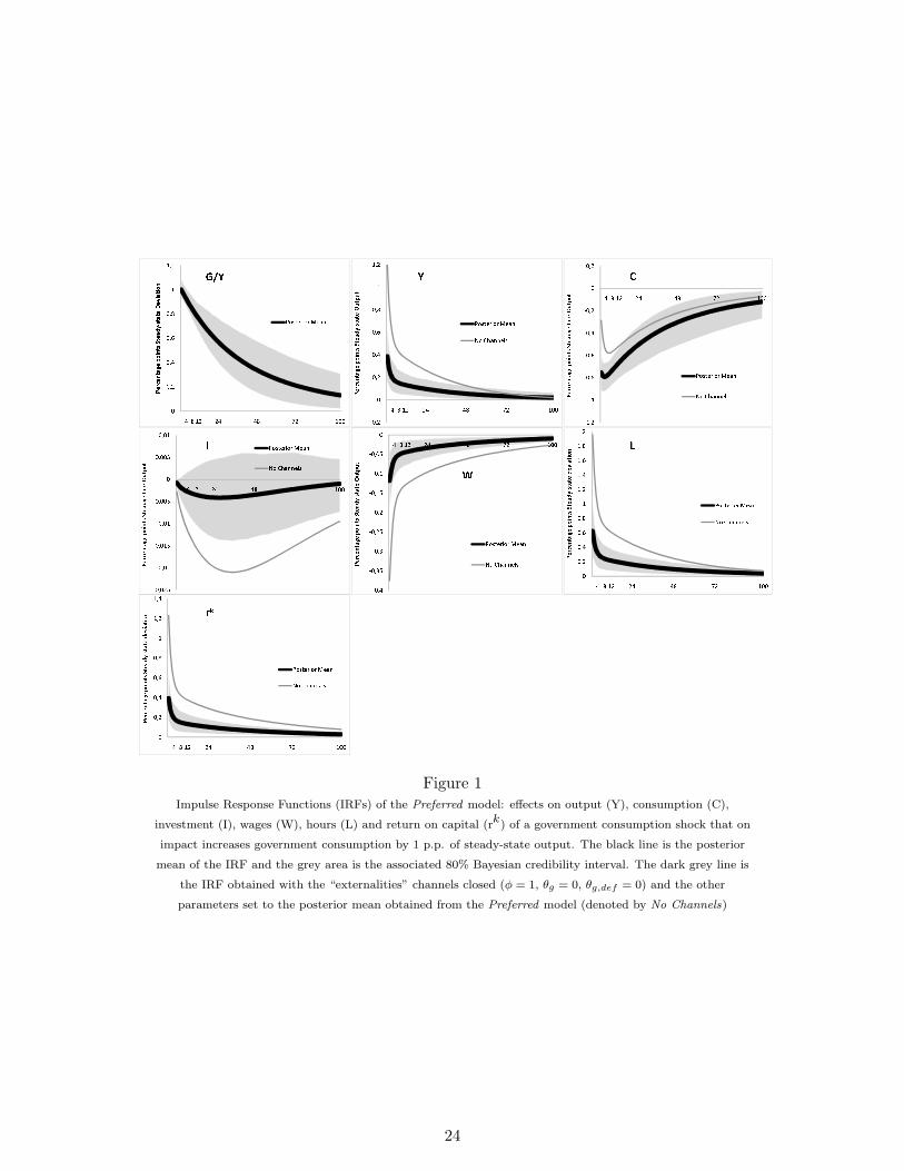
Focusing on the behavior of the variables in Figure 1, we can say that, because of substitutability,

the increase in government consumption lowers the marginal utility of consumption, leading households

10We note that in the case of a government consumption shock, the reported responses obtained with the Preferred modelare very similar to what obtains in the Productive Investment model.

11Hence, this restricted model is not estimated, in order to guarantee that the only parameters changing are those relatedto public spending externalities. However, we should note that the estimated posterior mean of the impulse response functionsobtained with the imposed restrictions are very similar to the reported ones.

22

to substitute part of their private consumption with the newly available government consumption. As a

consequence, private consumption (black line) decreases more than private consumption in the No Channels

specification (dark grey line). That is, in the Preferred model, both the negative wealth effect and the

substitutability effect sum up. Households work less in the Preferred framework since - for given negative

wealth effect - the marginal utility of consumption is lower than in the No Channels case. As a result, wages

decrease less in the Preferred case. To accommodate the new path for private consumption, the real interest

rate increases by less on impact, so that investment is crowed-out less than in the Preferred specification.

The impact on output is smaller in the Preferred model because of the lower increase in labor supply.

Quantitatively, the following numbers associated with the Preferred specification are worth referring: the

impact (mean) response of output amounts to 0.39 percentage points of steady state output, the one of

consumption reaches −0.79 percentage points of steady-state output after 3 quarters and the investment

reaction is virtually null.

23

-0,200,20,40,60,811,24 8 12 24 48 72 100Percentage points Steady-stat

e Output Y Posterior MeanNo Channels-1,2-1-0,8-0,6-0,4-0,200,2 4 8 12 24 48 72 100

Percentage points Steady-state Output C

Posterior MeanNo Channels-0,025-0,02-0,015-0,01-0,00500,0050,01 4 8 12 24 48 72 100Percentage points Steady-stat

e Output I Posterior MeanNo Channels-0,4-0,35-0,3-0,25-0,2-0,15-0,1-0,050 4 8 12 24 48 72 100

Percentage points Steady-state Output W Posterior MeanNo Channels 00,20,40,60,811,21,41,61,82

4 8 12 24 48 72 100Percentage points Steady-state deviation L Posterior MeanNo Channels

00,20,40,60,811,24 8 12 24 48 72 100Percentage points Steady-stat

e Deviation G/Y Posterior Mean

00,20,40,60,811,21,44 8 12 24 48 72 100Percentage points Steady-stat

e deviation rk Posterior MeanNo ChannelsFigure 1

Impulse Response Functions (IRFs) of the Preferred model: effects on output (Y), consumption (C),

investment (I), wages (W), hours (L) and return on capital (rk) of a government consumption shock that on

impact increases government consumption by 1 p.p. of steady-state output. The black line is the posterior

mean of the IRF and the grey area is the associated 80% Bayesian credibility interval. The dark grey line is

the IRF obtained with the “externalities” channels closed (ϕ = 1, θg = 0, θg,def = 0) and the other

parameters set to the posterior mean obtained from the Preferred model (denoted by No Channels)

24

-0,500,511,522,534 8 12 24 48 72 100Percentage points Steady-s

tate Output Y Posterior MeanNo Channels

-0,8-0,6-0,4-0,200,20,40,60,811,24 8 12 24 48 72 100Percentage points Steady-s

tate Output CPosterior MeanNo Channels -0,100,10,20,30,40,50,6

4 8 12 24 48 72 100Percentage points Steady-state Output I Posterior MeanNo Channels

-0,200,20,40,60,814 8 12 24 48 72 100Percentage points Steady-s

tate Output W Posterior MeanNo Channels00,20,40,60,811,21,41,61,8


00,20,40,60,811,24 8 12 24 48 72 100Percentage points Steady-s

tate Deviation IG/Y Posterior Mean

00,511,524 8 12 24 48 72 100Percentage points Steady-s

tate deviation rk Posterior MeanNo Channels

024681012

4 8 12 24 48 72 100Percentage points Steady-state deviation Public K Posterior Mean

-0,200,20,40,60,811,21,41,61,84 8 12 24 48 72 100Percentage points Steady-s

tate deviation Private K Posterior MeanNo Channels-0,500,511,522,534 8 12 24 48 72 100Percentage points Steady-s

tate Output Y Posterior MeanNo Channels

-0,8-0,6-0,4-0,200,20,40,60,811,24 8 12 24 48 72 100Percentage points Steady-s

tate Output CPosterior MeanNo Channels -0,100,10,20,30,40,50,6

4 8 12 24 48 72 100Percentage points Steady-state Output I Posterior MeanNo Channels

-0,4-0,200,20,40,60,814 8 12 24 48 72 100Percentage points Steady-s

tate Output W Posterior MeanNo Channels-0,200,20,40,60,811,21,41,61,8


00,20,40,60,811,24 8 12 24 48 72 100Percentage points Steady-s

tate Deviation IG/Y Posterior Mean

-0,500,511,524 8 12 24 48 72 100Percentage points Steady-s

tate deviation rk Posterior MeanNo Channels

-3-2,5-2-1,5-1-0,500,511,5 4 8 12 24 48 72 100Percentage points Steady-state deviation q

Posterior MeanNo Channels

024681012

4 8 12 24 48 72 100Percentage points Steady-state deviation Public K Posterior Mean

-0,200,20,40,60,811,21,41,61,84 8 12 24 48 72 100Percentage points Steady-s

tate deviation Private K Posterior MeanNo Channels

Figure 2Impulse Response Functions (IRFs) of the Productive Investment model: effects on output (Y), consumption

(C), investment (I), wages (W), hours (L), return on capital (rk), Tobin’s q (q), Private Capital (Private K)

and Public Capital Productivity (Public K) of a government investment shock that on impact increases

government investment by 1 p.p. of steady-state output. The black line is the posterior mean of the IRF and

the grey area is the associated 80% Bayesian credibility interval. The dark grey line is the IRF obtained with

the “externalities” channels closed (ϕ = 1, θg = 0, θg,def = 0) and the other parameters set to the posterior

mean obtained from the Productive Investment model (denoted by No Channels)

25

Turning the focus to Figure 2, we recall that, conditional on a positive value for θg, a non-defense

government investment shock contributes to enhance the productivity of private factors, creating a positive

wealth effect in the economy, ceteris paribus. As a result, in the Productive Investment economy the market

value of firms (labelled q) tends to increase (at least for some quarters), so firms are willing to invest more.

The positive wealth effect also fosters private consumption. Note that initially both consumption and Tobin’s

q go down on impact, due to the tension between two opposite forces operating in the economy: the negative

wealth effect created by government’s financing needs and the mentioned positive wealth effect. A rise in

private factors productivity entails a rise in labor input as the labor demand schedule shifts outwards. As

a consequence, both real wage and labor go up, ceteris paribus. However, note that the positive wealth

effect tends to lower labor supply. In our specific case, labor remains at a higher level in the Productive

Investment specification compared to the No Channels case. The response of output is positive on impact.

Furthermore, in the Productive Investment model, output tends to remain at a higher level with respect to

its steady state since public capital (productivity) and private capital build up and directly sustain output

growth. Note that in the No Channels specification output converges much sooner to the steady-state. The

quantitative analysis of the responses associated to the Productive Investment model reinforces the view

that the government investment shock releases its effects in the long run. The (mean) output response peaks

at 1.11 after 34 quarters, the one of consumption reaches 0.43 in quarter 59, and the investment response

peaks at 0.21 after 56 quarters. The long run properties of these effects are tightly linked to the estimated

persistence for the public investment process, which directly sustains the increase in the productivity of

public capital for many periods. Anyway, it is worth noting the width of the posterior interval, meaning

that the reactions can credibly take a large spectrum of values. For example, at the lower bound of the

credibility interval, output, consumption and investment reach the values of 0.18, 0.03 and 0.02, respectively.

The next section completes the quantitative analysis, resorting to the analysis of dynamic multipliers

induced by the public spending externalities.

4.4 Dynamic Multipliers

We analyze here public spending multipliers associated with the estimated effects of government spending

shocks on output, consumption and investment. We use the notion of present value multipliers formulated

in Mountford and Uhlig (2009); the present value multiplier of output, say, t quarters after an increase in

government consumption (or investment) is:

26

φt =

t∑k=0

(1 + rss)−kyk

t∑k=0

(1 + rss)−kgk

where yk represents the deviation of output from its steady-state and gk is government consumption (or

investment) measured as a fraction of steady-state output. rss is the steady-state real interest rate (net

of depreciation). The expression generalizes for the case of consumption and investment, in which case

deviations are expressed in units of steady-state output.

Tables VI and VII show the present value multipliers for Y , C and I and for various periods in response to

a government consumption and a government investment shock, conditional on the respective specification.

We look at the posterior mean of the multipliers and also at an 80% Bayesian credibility interval.

Looking at the multipliers produced by a government consumption shock (i.e. Table VI), we see that

the one related to output reaches its maximum, i.e. 0.39, on impact and then slowly decreases. The 80%

multiplier’s posterior interval contains most of the values found by Mountford and Uligh (2009), but are

lower than those found by Blanchard and Perotti (2002). Indeed, the first paper finds a multiplier’s range

between 0.44 and 0.23, the second one between 0.90 and 0.66, during the first 12 quarters, both within a VAR

framework. It is worth noting that the output multiplier calculated within the No Channels specification

results to be 1.21 on impact, i.e. three times bigger than the one in our Preferred economy. This discrepancy

holds quantitatively even if we directly estimate the No Channel specification; in this case, the posterior

mean of the output multiplier turns out to be 1.25. As expected, the multipliers for consumption and

investment are negative, though the 80% posterior interval for investment contains zero. In the case of

consumption the multipliers are clearly below those obtained in the No Channels model, especially at short

horizons, whereas for investment they are above, but still negative.12

Looking at the government investment multipliers, we underline their long-run characteristics, bearing

in mind that the strong estimated persistence of the government investment process is important to what

obtains. The output multiplier starts below 1, at 0.87, similar to the No Channels multiplier, but increases as

public capital productivity builds up, reaching 0.93 after three years and 1.44 after six. These values partially

overlap with the multipliers found by Perotti (2004), Leeper (2010) and Baxter and King (1993). The first

paper finds a multiplier ranging between 0.17 and 1.68 within the first five years. Leeper (2010)’s paper,

12It is worth noting that many of the analysis of the effects of government spending focus on military spending, instead ofgovernment consumption, as it is unlikely that this type of spending interacts with the business cycle. Among others, Barroand Redlick (2010) estimate an output multiplier ranging from 0.6 to 0.7 at the median unemployment rate (reaching 1.0 whenthe unemployment rate is around 12%); also, they find a crowding out for investment and net exports. Further, Hall (2009)’srange for the output multiplier is 0.7-1.0. Finally, Ramey (2011b), using news shocks obtained with a narrative approach, findsoutput multipliers in the range 0.6-1.2 (at peak GDP) and slightly negative consumption multipliers.

27

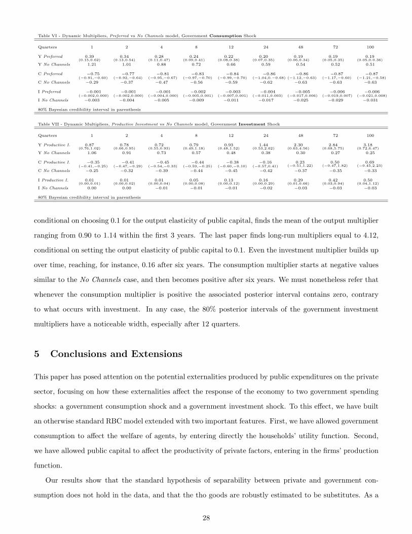
Table VI - Dynamic Multipliers, Preferred vs No Channels model, Government Consumption Shock

Quarters 1 2 4 8 12 24 48 72 100

Y Preferred 0.39(0.15,0.62)

0.34(0.13,0.54)

0.28(0.11,0.47)

0.24(0.09,0.41)

0.22(0.08,0.38)

0.20(0.07,0.35)

0.19(0.06,0.34)

0.19(0.05,0.35)

0.19(0.05,0.0.36)

Y No Channels 1.21 1.01 0.88 0.72 0.66 0.59 0.54 0.52 0.51

C Preferred −0.75(−0.91,−0.60)

−0.77(−0.92,−0.64)

−0.81(−0.95,−0.67)

−0.83(−0.97,−0.70)

−0.84(−0.99,−0.70)

−0.86(−1.04,0.−0.68)

−0.86(−1.12,−0.63)

−0.87(−1.17,−0.60)

−0.87(−1.21,−0.58)

C No Channels −0.29 −0.37 −0.47 −0.56 −0.59 −0.62 −0.63 −0.63 −0.63

I Preferred −0.001(−0.002,0.000)

−0.001(−0.002,0.000)

−0.001(−0.004,0.000)

−0.002(−0.005,0.001)

−0.003(−0.007,0.001)

−0.004(−0.011,0.003)

−0.005(−0.017,0.006)

−0.006(−0.019,0.007)

−0.006(−0.021,0.008)

I No Channels −0.003 −0.004 −0.005 −0.009 −0.011 −0.017 −0.025 −0.029 −0.031

80% Bayesian credibility interval in parenthesis

Table VII - Dynamic Multipliers, Productive Investment vs No Channels model, Government Investment Shock

Quarters 1 2 4 8 12 24 48 72 100

Y Productive I. 0.87(0.76,1.02)

0.78(0.66,0.95)

0.72(0.55,0.93)

0.79(0.49,1.18)

0.93(0.48,1.52)

1.44(0.53,2.62)

2.30(0.63,4.56)

2.84(0.68,5.75)

3.18(0.72,6.47)

Y No Channels 1.06 0.91 0.73 0.57 0.48 0.38 0.30 0.27 0.25

C Productive I. −0.35(−0.41,−0.25)

−0.41(−0.47,−0.29)

−0.45(−0.54,−0.33)

−0.44(−0.59,−0.25)

−0.38(−0.60,−0.10)

−0.16(−0.57,0.41)

0.23(−0.51,1.22)

0.50(−0.47,1.82)

0.69(−0.45,2.23)

C No Channels −0.25 −0.32 −0.39 −0.44 −0.45 −0.42 −0.37 −0.35 −0.33

I Productive I. 0.01(0.00,0.01)

0.01(0.00,0.02)

0.01(0.00,0.04)

0.05(0.00,0.08)

0.13(0.00,0.12)

0.16(0.00,0.29)

0.29(0.01,0.66)

0.42(0.03,0.94)

0.50(0.04,1.12)

I No Channels 0.00 0.00 −0.01 −0.01 −0.01 −0.02 −0.03 −0.03 −0.03

80% Bayesian credibility interval in parenthesis

conditional on choosing 0.1 for the output elasticity of public capital, finds the mean of the output multiplier

ranging from 0.90 to 1.14 within the first 3 years. The last paper finds long-run multipliers equal to 4.12,

conditional on setting the output elasticity of public capital to 0.1. Even the investment multiplier builds up

over time, reaching, for instance, 0.16 after six years. The consumption multiplier starts at negative values

similar to the No Channels case, and then becomes positive after six years. We must nonetheless refer that

whenever the consumption multiplier is positive the associated posterior interval contains zero, contrary

to what occurs with investment. In any case, the 80% posterior intervals of the government investment

multipliers have a noticeable width, especially after 12 quarters.

5 Conclusions and Extensions

This paper has posed attention on the potential externalities produced by public expenditures on the private

sector, focusing on how these externalities affect the response of the economy to two government spending

shocks: a government consumption shock and a government investment shock. To this effect, we have built

an otherwise standard RBC model extended with two important features. First, we have allowed government

consumption to affect the welfare of agents, by entering directly the households’ utility function. Second,

we have allowed public capital to affect the productivity of private factors, entering in the firms’ production

function.

Our results show that the standard hypothesis of separability between private and government con-

sumption does not hold in the data, and that the tho goods are robustly estimated to be substitutes. As a

28

consequence, the estimated response of private consumption to a government consumption shock is negative,

as in models where government investment is considered a pure waste (e.g. Baxter and King 1993 or Smets

and Wouters 2003), but the response is much stronger. Because of substitutability labor supply reacts less

to a government consumption shock, so the estimated output multiplier is lower (approximately one third)

than the one measured in models with separable government consumption. On the other hand, we find that

non-defense public investment enhances mildly, in some specifications, the productivity of private factors

while investment in defense appears not to have any such impact. When non-defense public investment

is found to shift the production frontier, shocks to it generate responses that manifest themselves only af-

ter several quarters: a positive reaction for private consumption, Tobin’s q, private investment and real

wages. Further, the estimated output multiplier builds up over time, in contrast with what obtains in the

corresponding model with unproductive government investment.

One potential extension of the present paper amounts to verifying whether our measures are affected

by several important features of fiscal policy, such as varying distortionary taxes, debt smoothing details,

implementation delays, or the zero lower bound on nominal interest rates. On other front, another significant

extension is related to the potential “composition” effect coming from the government consumption side.

Resorting to disaggregate government consumption data from 1947 onwards (Bureau of Economic Analysis),

it would be interesting to identify how each single category (e.g., administrative services, justice, health,

education and so on) is related - in preferences - with private consumption. Then, it would also be worth

assessing whether these potential relations vary over the business cycle.

29

References

[1] Ahmed, S. (1986), “Temporary and Permanent Government Spending in an Open Economy”, Journal

of Monetary Economics, 17 (3), 197-224.

[2] Amano, A.R. and T.S. Wirjanto (1998), “Government Expenditures and the Permanent-Income Model”,

Review of Economic Dynamics, 1 (3), 719-30.

[3] An, S. and F. Schorfheide (2007), “Bayesian Analysis of DSGE Models”, Econometric Reviews, 26 (2-4),

113-172.

[4] Aschauer, D. A. (1985), “Fiscal policy and aggregate demand”, American Economic Review, 75 (1),

117–127.

[5] Aschauer, D. A. (1989), “Is public expenditure productive?”, Journal of Monetary Economics, 23 (2),

177-200.

[6] Bailey, M. J. (1971), ”National Income and the Price Level: A Study in Macroeconomic Theory”, 2nd

Edition, New York: McGraw–Hill.

[7] Barro, R. (1981), “Output Effects of Government Purchases”, Journal of Political Economy, 89 (6),

1086-1121.

[8] Barro, R. and C. Redlick (2010), “Macroeconomic Effects from Government Purchases and Taxes”,

Harvard University, mimeo.

[9] Baxter, M. and R. G. King (1993), “Fiscal Policy in General Equilibrium”, American Economic Review,

83 (3), 315-334.

[10] Belo, F. and Yu, J. (2011), “Government Investment and the Stock Market”, University of Minnesota,

mimeo.

[11] Blanchard, O. J. and R. Perotti (2002), “An Empirical Characterization of the Dynamic Effects of

Changes in Government Spending and Taxes on Output”, Quarterly Journal of Economics, 117 (4),

1329-1368.

[12] Bouakez, H. and R. Rebei (2007), “Why Does Private Consumption Rise after a Government Spending

Shock?”, Canadian Journal of Economics, 40 (3), 954-979.

30

[13] Brooks, S. P. and A. Gelman (1998), “General Methods for Monitoring Convergence of Iterative Simu-

lations”, Journal of Computational and Graphical Statistics, 7 (4), 434-455.

[14] Chari, V. V., P. J. Kehoe and E. R. McGrattan (2009), ”New Keynesian Models: Not Yet Useful for

Policy Analysis”, American Economic Journal: Macroeconomics, 1 (1), 242-266.

[15] Christiano, L., M. Eichenbaum and C. Evans (2005), “Nominal Rigidities and the Dynamic Effects of

a Shock to Monetary Policy”, Journal of Political Economy, 113 (1), 1-45.

[16] Christiano, L., Eichenbaum, M.,Rebelo, S. (2011), “When is the Government Spending Multiplier

Large?”, Journal of Political Economy, 119 (1), 78-121.

[17] Finn, M. (1993), “Is All Government Capital Productive?”, mimeo Federal Reserve Bank of Richmond.

[18] Fiorito, R. and T. Kollitznas (2004), “Public goods, merit goods, and the relation between private and

government consumption”, European Economic Review, 48 (6), 1367-1398.

[19] Galı, J., J. D. Lopez-Salido and J. Valles (2007), ”Understanding the Effects of Government Spending

on Consumption,” Journal of the European Economic Association, 5 (1), 227-270.

[20] Geweke, J. F. (1999), “Using Simulation Methods for Bayesian Econometric Models: Inference, Devel-

opments and Communication”, Econometric Reviews, 18, 1-126.

[21] Hall, R. (2009), “By How Much Does GDP Rise if the Government Buys More Output?”, Brookings

Papers on Economic Activity.

[22] Karras, G. (1994), “Government spending and private consumption: Some international evidence”,

Journal of Money, Credit and Banking 26 (1), 9–22.

[23] King, R. G., Plosser, C. and Rebelo, S. T. (1988), “Production, growth and business cycles : I. The

basic neoclassical model,” Journal of Monetary Economics, 21 (2-3), 195-232.

[24] Leeper, E. M., Plante, M. and Traum, N. (2009), “Dynamics of Fiscal Financing in the United States”,

NBER Working Paper Series 15160.

[25] Leeper, E., Walker, T. B. and Yang, Shu-Chun S. (2010), “Government investment and fiscal stimulus”,

Journal of Monetary Economics, 57(8), 1000-1012.

[26] Linnemann, L. (2006), “The Effects of Government Spending on Private Consumption: A Puzzle?”,

Journal of Money, Credit, and Banking 38 (1), 1715-1736.

31

[27] Linnemann, L. and A. Schabert (2003), “Fiscal Policy in the New Neoclassical Synthesis”, Journal of

Money, Credit and Banking, 35 (6), 911-929.

[28] Monacelli T., R. Perotti, and A. Trigari (2010), “Unemployment fiscal multipliers”, Journal of Monetary

Economics, 57 (5), 531-553.

[29] Mountford A. and, H. Uhlig (2009), “What are the Effects of Fiscal Policy Shocks?”, Journal of Applied

Econometrics, 24 (6), 960-992.

[30] Perotti, R. (2004), ”Public Investment: Another (Different) Look”, Universita Bocconi, mimeo.

[31] Ramey, V. A. (2011a), ”Can Government Purchases Stimulate the Economy?”, Journal of Economic

Literature, 49 (3), 673-685.

[32] Ramey, V. A. (2011b), ”Identifying Government Spending Shocks: It’s all in the Timing”, The Quarterly

Journal of Economics, 126 (1), 1-50.

[33] Schmitt-Grohe, S. and Uribe, M. (2006), “Optimal Fiscal and Monetary Policy in a Medium-Scale

Macroeconomic Model”, NBER Macroeconomics Annual 2005, 20, 383-462.

[34] Smets, F. and R. Wouters (2003), “An Estimated Dynamic Stochastic General Equilibrium Model of

the Euro Area”, Journal of the European Economic Association, 1 (5), 1123-1175.

[35] Smets, F. and R. Wouters (2007), “Shocks and Frictions in US Business Cycles: A Bayesian DSGE

Approach”, American Economic Review, 97 (3), 586-606.

[36] Straub, R. and I. Tchakarov (2007), “Assesing the Impact of a Change in the Composition of Public

Spending: a Dsge Approach”, ECB Working Paper 479.

[37] Tatom, J. A. (1991), “Public capital and private sector performance”, Federal Reserve Bank of St. Louis

Review, 3-15.

[38] Uhlig, H. (2010), “Some fiscal calculus”, American Economic Review, 100 (2), 30–34.

[39] Walker, A.M. (1969), “On the Asymptotic Behaviour of Posterior Distributions”, Journal of the Royal

Statistical Society, 31 (2), 80-88.

32

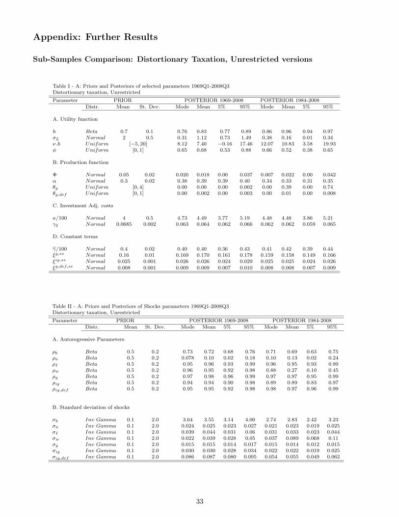
Appendix: Further Results

Sub-Samples Comparison: Distortionary Taxation, Unrestricted versions

Table I - A: Priors and Posteriors of selected parameters 1969Q1-2008Q3Distortionary taxation, Unrestricted

Parameter PRIOR POSTERIOR 1969-2008 POSTERIOR 1984-2008Distr. Mean St. Dev. Mode Mean 5% 95% Mode Mean 5% 95%

A. Utility function

h Beta 0.7 0.1 0.76 0.83 0.77 0.89 0.86 0.96 0.94 0.97σL Normal 2 0.5 0.31 1.12 0.73 1.49 0.38 0.16 0.01 0.34ν b Uniform [−5, 20] 8.12 7.40 −0.16 17.46 12.07 10.83 3.58 19.93ϕ Uniform [0, 1] 0.65 0.68 0.53 0.88 0.66 0.52 0.38 0.65


Φ Normal 0.05 0.02 0.020 0.018 0.00 0.037 0.007 0.022 0.00 0.042α Normal 0.3 0.02 0.38 0.39 0.39 0.40 0.34 0.33 0.31 0.35θg Uniform [0, 4] 0.00 0.00 0.00 0.002 0.00 0.39 0.00 0.74θg,def Uniform [0, 1] 0.00 0.002 0.00 0.003 0.00 0.01 0.00 0.008


κ/100 Normal 4 0.5 4.73 4.49 3.77 5.19 4.48 4.48 3.86 5.21γ2 Normal 0.0685 0.002 0.063 0.064 0.062 0.066 0.062 0.062 0.059 0.065

D. Constant terms


Table II - A: Priors and Posteriors of Shocks parameters 1969Q1-2008Q3Distortionary taxation, Unrestricted

Parameter PRIOR POSTERIOR 1969-2008 POSTERIOR 1984-2008Distr. Mean St. Dev. Mode Mean 5% 95% Mode Mean 5% 95%





33

Post-1984 Sample: Preferred (θg = θg,def = 0) vs. Unrestricted specification

Table I - B Priors and Posteriors of selected parameters 1984Q1-2008Q3Preferred specification vs. Unrestricted

Parameter PRIOR POSTERIOR POSTERIORθg = θg,def = 0 Unrestricted


A. Utility function

h Beta 0.7 0.1 0.85 0.94 0.93 0.96 0.86 0.96 0.94 0.97σL Normal 2 0.5 0.35 0.17 0.01 0.37 0.38 0.16 0.01 0.34ν b Uniform [−5, 20] 8.91 14.3 2.44 26.5 12.07 10.83 3.58 19.93ϕ Uniform [0, 1] 0.66 0.47 0.36 0.58 0.66 0.52 0.38 0.65


Φ Normal 0.05 0.02 0.007 0.014 0.00 0.028 0.007 0.022 0.00 0.042α Normal 0.3 0.02 0.34 0.33 0.31 0.35 0.34 0.33 0.31 0.35θg Uniform [0, 4] - - - - 0.00 0.39 0.00 0.74θg,def Uniform [0, 1] - - - - 0.00 0.01 0.00 0.008


κ/100 Normal 4 0.5 4.50 4.84 4.16 5.51 4.48 4.48 3.86 5.21γ2 Normal 0.0685 0.002 0.062 0.061 0.058 0.064 0.062 0.062 0.059 0.065

D. Constant terms


Table II - B Priors and Posteriors of Shocks parameters 1984Q1-2008Q3Preferred specification vs. Unrestricted

Parameter PRIOR POSTERIOR POSTERIORθg = θg,def = 0 Unrestricted






34

Appendix: Equilibrium conditions with transformed variables

We restric attention to the model with distortionary taxation. The version with lump-sum taxation obtains

with all marginal tax rates equal to zero. Equilibrium conditions follow from the first order conditions

(F.O.C.s) of households’ and firms’ problems while imposing symmetry, fiscal policy equations, market

clearing conditions and processes for the exogenous processes. We then stationarize the variables Ct, It, Kt,

Wt , Taxt, Tt, Gt, Igt and Ig,deft dividing them by the level of technology, At. Lower case letters indicates

transformed variables. The same treatment is required for the Lagrange multipliers associated with the

budget constraint and the capital accumulation equation, respectively λt and qt (Tobin’s q).

• Aggregator (consumption):

ct =[ϕ (ct)

v−1v + (1− ϕ) (gt)

v−1v

] vv−1

(27)

• Consumption F.O.C.:

(1 + τ c)λt exp(−(γ + εat )) = eεbt

[ϕ

(ctct

) 1v [

(ct exp(γ + εat )− γct−1)−1

]](28)

• Labor supply F.O.C.:

λt =χLσn

t

(1− τw)wt(29)

• Investment F.O.C.:

λt = λtqtEt

{[1− κ

2

(eε

Itit exp(γ + εat )

it−1− eγ

)2]− it

it−1exp(γ + εat )κe

εIt

(eε


it−1− eγ

)}+

(30)

+ βEt

[λt+1qt+1 exp(−(γ + εat+1))

(eε

It+1

it+1 exp(γ + εat+1)

it

)2

κeεIt+1

(eε

it+1

it+1 exp(γ + εat+1)

it− eγ

)]

35

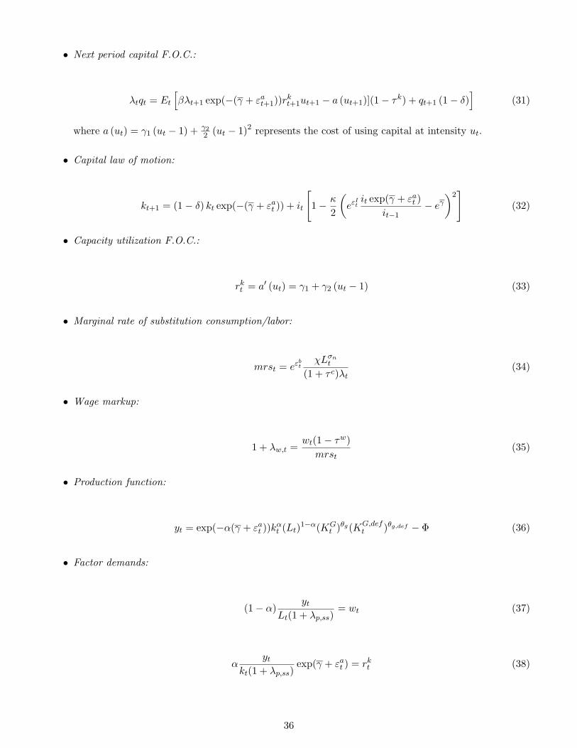
• Next period capital F.O.C.:

λtqt = Et

[βλt+1 exp(−(γ + εat+1))r

kt+1ut+1 − a (ut+1)](1− τk) + qt+1 (1− δ)

](31)

where a (ut) = γ1 (ut − 1) + γ22 (ut − 1)2 represents the cost of using capital at intensity ut.

• Capital law of motion:

kt+1 = (1− δ) kt exp(−(γ + εat )) + it

[1− κ

2

(eε


it−1− eγ

)2]

(32)

• Capacity utilization F.O.C.:

rkt = a′ (ut) = γ1 + γ2 (ut − 1) (33)

• Marginal rate of substitution consumption/labor:

mrst = eεbt

χLσnt

(1 + τ c)λt(34)

• Wage markup:

1 + λw,t =wt(1− τw)

mrst(35)

• Production function:

yt = exp(−α(γ + εat ))kαt (Lt)

1−α(KGt )θg(KG,def

t )θg,def − Φ (36)

• Factor demands:

(1− α)yt

Lt(1 + λp,ss)= wt (37)

αyt

kt(1 + λp,ss)exp(γ + εat ) = rkt (38)

36

• Marginal cost:

MCt =

(rkt)α

w1−αt

αα (1− α)1−α ∗ 1

(KGt )θg(KG,def

t )θg,def(39)

• Price markup:

1

MCt= 1 + λp,ss (40)

• Evolution of the productivity of public capital:

KGt+1 = (1− δKg)K

Gt + ξigt (41)

where ξigt = igt /yt = exp(εigt + ssig)/(1 + exp(εigt + ssig)) and ssig = log(ξig,ss/(1− ξig,ss))

KG,deft+1 = (1− δKg,def )K

G,deft + ξig,deft (42)

where ξig,deft = ig,deft /yt = exp(εig,deft +ssig,def )/(1+exp(εig,deft +ssig,def )) and ssig,def = log(ξig,def,ss/(1−

ξig,def,ss))

• Government consumption:

ξgt = gt/yt = exp(εgt + ssg)/(1 + exp(εgt + ssg)) (43)

where ssg = log(ξg,ss/(1− ξg,ss))

• Balanced government budget:

τ cct + τwwtLt + τk[rkt ut − a (ut)

]kt + tt = ξgt yt + ξigt yt + ξig,deft yt (44)

37

• Shocks processes:

εbt = ρbεbt−1 + ηbt (45)

εIt = ρiεIt−1 + ηIt

εat = ρaεat−1 + ηat

λw,t = (1− ρw)λw,ss + ρwλw,t−1 + ηwt

εgt = ρgεgt−1 + ηgt

εigt = ρigεiigt−1 + ηigt

εig,deft = ρig,defεiig,deft−1 + ηig,deft

Appendix: Bayesian inference

The following characterizes briefly the estimation procedure. The model is solved up to a log-linear ap-

proximation around the deterministic steady state. Once the solution is obtained, the model can be cast in

state-space form, and the likelihood function can be computed using the Kalman filter. In every variation we

start by finding the mode of the posterior distribution, or the parameter vector θM maximizing P (θ|YT ,m).

Initial values in the numerical algorithms are sometimes important so we repeated the procedure using vari-

ous initial values in order to guarantee as much as possible that the mode is indeed found. Only then we ran

the Metropolis-Hastings algorithm using 3.105 iterations while monitoring its convergence. Specifically, we

use the Random-Walk Metropolis algorithm which generates Markov chains with stationary distributions

that correspond to the the posterior distribution of interest. Practically, we strictly follow the procedure

described in section 4.1 of An and Schorfheide (2007).

That said, the following information regarding our specific estimation is worth noting. First, the accep-

tation rate in the Metropolis-Hastings algorithm is around 25%. Second, we monitor the convergence of the

Markov Chain generated by the Metropolis Hastings algorithm to the posterior distribution of interest by

using the diagnostics proposed by Brooks and Gelman (1998). Intuitively, different Markov Chain sequences

obtained with the algorithm should be similar once the effects of starting values vanish. Hence, second mo-

ments of the parameters calculated across sequences should not differ much from second moments calculated

within a sequence. Using a rule-of-thumb that the two moments are equal if their difference is below 20%,

should ensure convergence. If this is not the case, either the effect of the initial replications has not worn

38

off, or the number of draws taken is too low. In our case, the number of draws we use is sufficient to achieve

convergence.

Appendix: Data

We follow closely Smets and Wouters (2007) in treating the data. We use the September 30, 2010 vintage

of data. The tables below clarify sources and transformations.

Table D1 - Data Sources

Variable Designation Source CODE

Gross Domestic Product (Nominal) GDP US Dep. of Commerce - BEA A191RC1Personal Cons. Expenditures (Nominal) C US Dep. of Commerce - BEA DPCERC1Personal Cons.Expenditures - Durables (Nominal) Durables US Dep. of Commerce - BEA DDURRC1Private Fixed Domestic Investment (Nominal) PFI US Dep. of Commerce - BEA A007RC1Federal Cons. Expenditures (Nominal) G Federal US Dep. of Commerce - BEA A957RC1State & Local Cons. Expenditures (Nominal) G StateLocal US Dep. of Commerce - BEA A991RC1Federal Gross Investment, Non-Defense (Nominal) IG Federal US Dep. of Commerce - BEA A798RC1Federal Gross Investment, Defense (Nominal) IG Defense US Dep. of Commerce - BEA A788RC1State & Local Gross Investment (Nominal) IG StateLocal US Dep. of Commerce - BEA A799RC1Gross Domestic Product Deflator GDPDEF US Dep. of Commerce - BEA GDPDEFHourly Compensation, Non Farm Sector (Nominal) Wages Bureau of Labor Statistics PRS85006103Civilian noninstitutional population, 16 years and over POPULATION Bureau of Labor Statistics LNU00000000Q

All series are seasonally adjusted at annual rates

Table D2 - Observables for measurement equations

Y obst =(GDP/GDPDEF)/POPULATION

Cobst =((C-Durables)/GDPDEF)/POPULATION

Iobst =((PFI+Durables)/GDPDEF)/POPULATIONW obs

t =(Wages/GDPDEF)/POPULATION

ξg,obst =(G Federal+G StateLocal)/GDP

ξigt =(IG Federal+IG StateLocal)/GDP

ξig,def,obst =IG Defense/GDP

39

Banco de Portugal | Working Papers i

WORKING PAPERS

2010

1/10 MEASURING COMOVEMENT IN THE TIME-FREQUENCY SPACE — António Rua

2/10 EXPORTS, IMPORTS AND WAGES: EVIDENCE FROM MATCHED FIRM-WORKER-PRODUCT PANELS — Pedro S. Martins, Luca David Opromolla

3/10 NONSTATIONARY EXTREMES AND THE US BUSINESS CYCLE — Miguel de Carvalho, K. Feridun Turkman, António Rua

4/10 EXPECTATIONS-DRIVEN CYCLES IN THE HOUSING MARKET — Luisa Lambertini, Caterina Mendicino, Maria Teresa Punzi

5/10 COUNTERFACTUAL ANALYSIS OF BANK MERGERS — Pedro P. Barros, Diana Bonfi m, Moshe Kim, Nuno C. Martins

6/10 THE EAGLE. A MODEL FOR POLICY ANALYSIS OF MACROECONOMIC INTERDEPENDENCE IN THE EURO AREA — S. Gomes, P. Jacquinot, M. Pisani

7/10 A WAVELET APPROACH FOR FACTOR-AUGMENTED FORECASTING — António Rua

8/10 EXTREMAL DEPENDENCE IN INTERNATIONAL OUTPUT GROWTH: TALES FROM THE TAILS — Miguel de Carvalho, António Rua

9/10 TRACKING THE US BUSINESS CYCLE WITH A SINGULAR SPECTRUM ANALYSIS — Miguel de Carvalho, Paulo C. Rodrigues, António Rua

10/10 A MULTIPLE CRITERIA FRAMEWORK TO EVALUATE BANK BRANCH POTENTIAL ATTRACTIVENESS — Fernando A. F. Ferreira, Ronald W. Spahr, Sérgio P. Santos, Paulo M. M. Rodrigues

11/10 THE EFFECTS OF ADDITIVE OUTLIERS AND MEASUREMENT ERRORS WHEN TESTING FOR STRUCTURAL BREAKS IN VARIANCE

— Paulo M. M. Rodrigues, Antonio Rubia

12/10 CALENDAR EFFECTS IN DAILY ATM WITHDRAWALS — Paulo Soares Esteves, Paulo M. M. Rodrigues

13/10 MARGINAL DISTRIBUTIONS OF RANDOM VECTORS GENERATED BY AFFINE TRANSFORMATIONS OF INDEPENDENT TWO-PIECE NORMAL VARIABLES

— Maximiano Pinheiro

14/10 MONETARY POLICY EFFECTS: EVIDENCE FROM THE PORTUGUESE FLOW OF FUNDS — Isabel Marques Gameiro, João Sousa

15/10 SHORT AND LONG INTEREST RATE TARGETS — Bernardino Adão, Isabel Correia, Pedro Teles

16/10 FISCAL STIMULUS IN A SMALL EURO AREA ECONOMY — Vanda Almeida, Gabriela Castro, Ricardo Mourinho Félix, José Francisco Maria

17/10 FISCAL INSTITUTIONS AND PUBLIC SPENDING VOLATILITY IN EUROPE — Bruno Albuquerque

Banco de Portugal | Working Papers ii

18/10 GLOBAL POLICY AT THE ZERO LOWER BOUND IN A LARGE-SCALE DSGE MODEL — S. Gomes, P. Jacquinot, R. Mestre, J. Sousa

19/10 LABOR IMMOBILITY AND THE TRANSMISSION MECHANISM OF MONETARY POLICY IN A MONETARY UNION — Bernardino Adão, Isabel Correia

20/10 TAXATION AND GLOBALIZATION — Isabel Correia

21/10 TIME-VARYING FISCAL POLICY IN THE U.S. — Manuel Coutinho Pereira, Artur Silva Lopes

22/10 DETERMINANTS OF SOVEREIGN BOND YIELD SPREADS IN THE EURO AREA IN THE CONTEXT OF THE ECONOMIC AND FINANCIAL CRISIS

— Luciana Barbosa, Sónia Costa

23/10 FISCAL STIMULUS AND EXIT STRATEGIES IN A SMALL EURO AREA ECONOMY — Vanda Almeida, Gabriela Castro, Ricardo Mourinho Félix, José Francisco Maria

24/10 FORECASTING INFLATION (AND THE BUSINESS CYCLE?) WITH MONETARY AGGREGATES — João Valle e Azevedo, Ana Pereira

25/10 THE SOURCES OF WAGE VARIATION: AN ANALYSIS USING MATCHED EMPLOYER-EMPLOYEE DATA — Sónia Torres,Pedro Portugal, John T.Addison, Paulo Guimarães

26/10 THE RESERVATION WAGE UNEMPLOYMENT DURATION NEXUS — John T. Addison, José A. F. Machado, Pedro Portugal

27/10 BORROWING PATTERNS, BANKRUPTCY AND VOLUNTARY LIQUIDATION — José Mata, António Antunes, Pedro Portugal

28/10 THE INSTABILITY OF JOINT VENTURES: LEARNING FROM OTHERS OR LEARNING TO WORK WITH OTHERS — José Mata, Pedro Portugal

29/10 THE HIDDEN SIDE OF TEMPORARY EMPLOYMENT: FIXED-TERM CONTRACTS AS A SCREENING DEVICE — Pedro Portugal, José Varejão

30/10 TESTING FOR PERSISTENCE CHANGE IN FRACTIONALLY INTEGRATED MODELS: AN APPLICATION TO WORLD INFLATION RATES

— Luis F. Martins, Paulo M. M. Rodrigues

31/10 EMPLOYMENT AND WAGES OF IMMIGRANTS IN PORTUGAL — Sónia Cabral, Cláudia Duarte

32/10 EVALUATING THE STRENGTH OF IDENTIFICATION IN DSGE MODELS. AN A PRIORI APPROACH — Nikolay Iskrev

33/10 JOBLESSNESS — José A. F. Machado, Pedro Portugal, Pedro S. Raposo

2011

1/11 WHAT HAPPENS AFTER DEFAULT? STYLIZED FACTS ON ACCESS TO CREDIT — Diana Bonfi m, Daniel A. Dias, Christine Richmond

2/11 IS THE WORLD SPINNING FASTER? ASSESSING THE DYNAMICS OF EXPORT SPECIALIZATION — João Amador

Banco de Portugal | Working Papers iii

3/11 UNCONVENTIONAL FISCAL POLICY AT THE ZERO BOUND — Isabel Correia, Emmanuel Farhi, Juan Pablo Nicolini, Pedro Teles

4/11 MANAGERS’ MOBILITY, TRADE STATUS, AND WAGES — Giordano Mion, Luca David Opromolla

5/11 FISCAL CONSOLIDATION IN A SMALL EURO AREA ECONOMY — Vanda Almeida, Gabriela Castro, Ricardo Mourinho Félix, José Francisco Maria

6/11 CHOOSING BETWEEN TIME AND STATE DEPENDENCE: MICRO EVIDENCE ON FIRMS’ PRICE-REVIEWING STRATEGIES

— Daniel A. Dias, Carlos Robalo Marques, Fernando Martins

7/11 WHY ARE SOME PRICES STICKIER THAN OTHERS? FIRM-DATA EVIDENCE ON PRICE ADJUSTMENT LAGS — Daniel A. Dias, Carlos Robalo Marques, Fernando Martins, J. M. C. Santos Silva

8/11 LEANING AGAINST BOOM-BUST CYCLES IN CREDIT AND HOUSING PRICES — Luisa Lambertini, Caterina Mendicino, Maria Teresa Punzi

9/11 PRICE AND WAGE SETTING IN PORTUGAL LEARNING BY ASKING — Fernando Martins

10/11 ENERGY CONTENT IN MANUFACTURING EXPORTS: A CROSS-COUNTRY ANALYSIS — João Amador

11/11 ASSESSING MONETARY POLICY IN THE EURO AREA: A FACTOR-AUGMENTED VAR APPROACH — Rita Soares

12/11 DETERMINANTS OF THE EONIA SPREAD AND THE FINANCIAL CRISIS — Carla Soares, Paulo M. M. Rodrigues

13/11 STRUCTURAL REFORMS AND MACROECONOMIC PERFORMANCE IN THE EURO AREA COUNTRIES: A MODEL-BASED ASSESSMENT

— S. Gomes, P. Jacquinot, M. Mohr, M. Pisani

14/11 RATIONAL VS. PROFESSIONAL FORECASTS — João Valle e Azevedo, João Tovar Jalles

15/11 ON THE AMPLIFICATION ROLE OF COLLATERAL CONSTRAINTS — Caterina Mendicino

16/11 MOMENT CONDITIONS MODEL AVERAGING WITH AN APPLICATION TO A FORWARD-LOOKING MONETARY POLICY REACTION FUNCTION

— Luis F. Martins

17/11 BANKS’ CORPORATE CONTROL AND RELATIONSHIP LENDING: EVIDENCE FROM RETAIL LOANS — Paula Antão, Miguel A. Ferreira, Ana Lacerda

18/11 MONEY IS AN EXPERIENCE GOOD: COMPETITION AND TRUST IN THE PRIVATE PROVISION OF MONEY — Ramon Marimon, Juan Pablo Nicolini, Pedro Teles

19/11 ASSET RETURNS UNDER MODEL UNCERTAINTY: EVIDENCE FROM THE EURO AREA, THE U.K. AND THE U.S. — João Sousa, Ricardo M. Sousa

20/11 INTERNATIONAL ORGANISATIONS’ VS. PRIVATE ANALYSTS’ FORECASTS: AN EVALUATION — Ildeberta Abreu

21/11 HOUSING MARKET DYNAMICS: ANY NEWS? — Sandra Gomes, Caterina Mendicino

Banco de Portugal | Working Papers iv

22/11 MONEY GROWTH AND INFLATION IN THE EURO AREA: A TIME-FREQUENCY VIEW — António Rua

23/11 WHY EX(IM)PORTERS PAY MORE: EVIDENCE FROM MATCHED FIRM-WORKER PANELS — Pedro S. Martins, Luca David Opromolla

24/11 THE IMPACT OF PERSISTENT CYCLES ON ZERO FREQUENCY UNIT ROOT TESTS — Tomás del Barrio Castro, Paulo M.M. Rodrigues, A.M. Robert Taylor

25/11 THE TIP OF THE ICEBERG: A QUANTITATIVE FRAMEWORK FOR ESTIMATING TRADE COSTS — Alfonso Irarrazabal, Andreas Moxnes, Luca David Opromolla

26/11 A CLASS OF ROBUST TESTS IN AUGMENTED PREDICTIVE REGRESSIONS — Paulo M.M. Rodrigues, Antonio Rubia

27/11 THE PRICE ELASTICITY OF EXTERNAL DEMAND: HOW DOES PORTUGAL COMPARE WITH OTHER EURO AREA COUNTRIES?

— Sónia Cabral, Cristina Manteu

28/11 MODELING AND FORECASTING INTERVAL TIME SERIES WITH THRESHOLD MODELS: AN APPLICATION TO S&P500 INDEX RETURNS

— Paulo M. M. Rodrigues, Nazarii Salish

29/11 DIRECT VS BOTTOM-UP APPROACH WHEN FORECASTING GDP: RECONCILING LITERATURE RESULTS WITH INSTITUTIONAL PRACTICE

— Paulo Soares Esteves

30/11 A MARKET-BASED APPROACH TO SECTOR RISK DETERMINANTS AND TRANSMISSION IN THE EURO AREA — Martín Saldías

31/11 EVALUATING RETAIL BANKING QUALITY SERVICE AND CONVENIENCE WITH MCDA TECHNIQUES: A CASE STUDY AT THE BANK BRANCH LEVEL

— Fernando A. F. Ferreira, Sérgio P. Santos, Paulo M. M. Rodrigues, Ronald W. Spahr

2012

1/12 PUBLIC-PRIVATE WAGE GAPS IN THE PERIOD PRIOR TO THE ADOPTION OF THE EURO: AN APPLICATION BASED ON LONGITUDINAL DATA

— Maria Manuel Campos, Mário Centeno

2/12 ASSET PRICING WITH A BANK RISK FACTOR — João Pedro Pereira, António Rua

3/12 A WAVELET-BASED ASSESSMENT OF MARKET RISK: THE EMERGING MARKETS CASE — António Rua, Luis C. Nunes

4/12 COHESION WITHIN THE EURO AREA AND THE U. S.: A WAVELET-BASED VIEW — António Rua, Artur Silva Lopes

5/12 EXCESS WORKER TURNOVER AND FIXED-TERM CONTRACTS: CAUSAL EVIDENCE IN A TWO-TIER SYSTEM — Mário Centeno, Álvaro A. Novo

6/12 THE DYNAMICS OF CAPITAL STRUCTURE DECISIONS — Paula Antão, Diana Bonfi m

7/12 QUANTILE REGRESSION FOR LONG MEMORY TESTING: A CASE OF REALIZED VOLATILITY — Uwe Hassler, Paulo M. M. Rodrigues, Antonio Rubia

Banco de Portugal | Working Papers v

8/12 COMPETITION IN THE PORTUGUESE ECONOMY: AN OVERVIEW OF CLASSICAL INDICATORS — João Amador, Ana Cristina Soares

9/12 MARKET PERCEPTION OF FISCAL SUSTAINABILITY: AN APPLICATION TO THE LARGEST EURO AREA ECONOMIES — Maximiano Pinheiro

10/12 THE EFFECTS OF PUBLIC SPENDING EXTERNALITIES — Valerio Ercolani, João Valle e Azevedo

The Effects of Public Spending Externalities Publications Research/wp201210.… · Assessing the...

Documents

Transcript of The Effects of Public Spending Externalities Publications Research/wp201210.… · Assessing the...