The Effects of Maternal Employment on the

Health of School-Age Children∗

Melinda Sandler Morrill

Department of EconomicsUniversity of Maryland, College ParkEmail: melinda.morrill@gmail.com

Job Market Paper

This Version: January 11, 2008

Abstract

Over the past several decades, an increasing number of women with children participated inthe labor force. This has led researchers from a variety of disciplines to consider the impact ofmaternal employment on children, including the effects of maternal employment on children’shealth. The net effects are theoretically ambiguous given that maternal employment increasesfamily income and access to health insurance but places additional burdens on a mother’s time.Empirical identification is difficult because a mother’s choice to participate in the labor market isendogenous. For example, a child’s health may directly affect a mother’s labor supply decision, ora mother’s choice to work may be indicative of the mother’s preferences and skills. In this paper, Iimplement an instrumental variables strategy using pooled data from the restricted version of theNational Health Interview Survey (1985-2004). I identify the effects of maternal employment onovernight hospitalizations, emergency room visits, asthma episodes, and injuries and poisoningsfor children ages seven to seventeen. The conditional correlations between maternal employmentand each of these four health events are zero or negative, suggesting that, if anything, havinga mother that works is associated with a lower risk of a child having a bad health episode. Imeasure the causal effect of maternal employment on the health of children by using exogenousvariation in each child’s youngest sibling’s eligibility for kindergarten as an instrument. I showthat having a mother that works actually increases the probability a child will have a negativehealth episode. The results point to a consistent effect for all four outcomes and are statisticallysignificant for overnight hospitalizations, injuries and poisonings, and asthma episodes. I provideevidence that this effect is not a reflection of a non-representative local average treatment effectand is robust to specification checks.

∗This work was supported by AHRQ Dissertation Research Fellowship Grant R36HS017375-01. I would especiallylike to thank Judith Hellerstein for all of her guidance and support. I am also grateful to Mark Duggan, Bill Evans,Thayer Morrill, Marianne Bitler, Jonah Gelbach, Steven Stillman, Amanda Geller, Scott Imberman, and MelissaMcInerney for helpful discussions and suggestions. All errors remaining are my own.

1 Introduction

Over the past several decades, an increasing number of women with children participated in the

labor force. According to a Bureau of Labor Statistics report (2006), in 1975 54.9 percent of

women with children ages six to seventeen were in the civilian labor force. By 2001 that number

had risen to 79.4, although it fell slightly to 76.9 in 2005. The economic impact of women’s

labor force participation cannot be completely characterized without understanding all of the costs

and benefits involved. In particular, a woman’s labor force participation might impact the health

and well-being of her children. Not only does poor child health have contemporaneous economic

consequences, such as health care expenditures and utilization, but poor health may also hinder a

child’s cognitive development (see, e.g., Blau and Grossberg, 1992). In addition, a growing amount

of research finds that experiences during childhood can affect adult health,1 adult economic and

social well-being,2 and even longevity,3 so a woman’s participation in the labor market might have

long lasting effects on her children.

The direction and magnitude of the effect of maternal labor supply on child health is theoret-

ically ambiguous. The clearest mechanism through which maternal employment might positively

impact children is through an increase in family income. There is a well established income-health

gradient, which has been shown to exist for children as well as adults (see Case, Lubotsky, and

Paxson, 2002, and Currie and Lin, 2007). More income allows families to increase investments in

health for their children, including better diet and better health care. In addition, some mothers

acquire or improve their family’s health insurance coverage due to their employment. However, ma-

ternal employment imposes a burden on a mother’s time and may result in the poorer supervision

or care of her children. A child’s health is at least partially a function of time-intensive activities

such as healthy meal preparation and house cleaning. A working mother may have less time to

allocate to these types of activities. Bianchi (2000) shows that working mothers spend less time

doing housework, and Crepinsek et al. (2004) document that children of working mothers have

lower overall “Healthy Eating Index” scores. In addition, a child whose mother works may be left

unsupervised or less-supervised more often than if the mother were at home full-time.

Previous studies on the effects of maternal employment find little measurable impact on child

health, as discussed further in Section 2. Empirical identification of the effect is difficult because

a mother’s choice to participate in the labor market is endogenous. Maternal employment has

often been considered as the effect of, not the cause of, the family’s characteristics.4 Mothers with1Dietz, 1997.2Case and Paxson, 2006 and Case, Fertig, and Paxson, 2005.3Lleras-Muney, 2006.4There is a substantial literature estimating the effect of child morbidity and disability on maternal employment.

For example, Powers (2001 and 2003) argues that when a child is unhealthy, some mothers reduce their labor supply.Gould (2004) shows that a mother reduces her labor supply if her child has a time intensive disability but increasesher labor supply if her child has a high-cost disability. Corman et al. (2004) find that having an unhealthy child

1

healthy children may find it easier to work, whereas mothers of children with special needs may

find it difficult to work outside of the home. Alternatively, having a child with a chronic condition

may make it necessary for a mother to work in order to provide health insurance or additional

income for her family. Isolating the effect of a mother’s labor force participation on the health and

well-being of her children is confounded by this reverse relationship: a child’s health may directly

affect a mother’s labor supply decision.

In addition, a mother’s choice to work or not may indicate something about the mother’s

(unobserved) preferences and skills. If a mother’s decision to work indicates something about her

general ability level, motivation, inclinations, skill at caretaking, etc., then the sample of working

mothers may not be a random sample of all mothers. This might lead to a spurious correlation

between maternal labor supply and child health. This particular concern has prompted researchers

to employ fixed effects strategies that can capture unobserved mother (and sometimes child-specific)

characteristics (Ruhm, 2004). However, this methodology can only account for the unobserved

characteristics that are constant over time. This may be problematic given the reverse relationship

described above if children’s health itself changes over time. In this study, I employ an instrumental

variables strategy to isolate the causal effect of maternal employment, overcoming this limitation

of fixed effects analysis.

In the absence of a perfect measure of underlying child health, I analyze the effects of maternal

employment on four health outcomes: overnight hospitalizations, emergency room visits, asthma

episodes, and injuries and poisonings. These outcomes capture both acute and chronic conditions.

As argued in Section 3.3, while none of these outcomes alone are perfect, when taken together

they provide a good proxy for child health. Together the effects of maternal employment on these

four health outcomes, presented in Section 5, provide compelling evidence of a true effect on child

health.

Consistent with much of the existing literature, I find that the conditional correlations between

maternal employment and each of the child health episodes, as estimated using ordinary least

squares regressions, are zero or negative. That is, having a working mother is associated with a

lower risk of a child having the health incident. Because of the endogeneity of maternal employment,

however, these correlations do not necessarily represent a causal relationship. In this paper, I use

an instrumental variables strategy where the instrument relies on the fact that the opportunity cost

of a woman working is substantially lowered when her youngest child becomes eligible for public

school, potentially leading to an increase in maternal labor supply at that time. I measure the

health of children ages seven through seventeen years old that have at least one younger sibling. I

reduces a mother’s probability of working by around 8 percentage points. Duggan and Kearney (2007) investigatethe effects of a child’s enrollment in the federal Supplemental Security Income program (SSI) on his/her family andfind little direct effect on maternal employment. Norberg (1998) looks at outcomes at birth to determine maternalemployment in first year of life. She argues that it is not daycare that affects child health and development but thatchild health affects a mother’s decision to work.

2

further restrict the estimation sample to children whose youngest sibling is within a specified age

range around five years old. I use each child’s youngest sibling’s eligibility for kindergarten as an

instrument for maternal labor supply in assessing the causal impact of maternal labor supply on

the health of the older child. As discussed further below, Gelbach (2002) established that a child’s

eligibility for kindergarten, as measured by quarter of birth, increases maternal employment. I

argue that a child’s youngest sibling’s eligibility for kindergarten provides variation in maternal

employment that is plausibly exogenous to the older child’s health. Nonetheless, in Sections 3

and 5 I provide discussions of the potential biases associated with this instrument. I also explore

whether there is treatment effect heterogeneity across major demographic categories, and I discuss

the generalizability of the estimated local average treatment effect measured by the instrumental

variables strategy.

My estimates suggest that maternal employment increases the probability a child will have a

negative health episode. The estimates are large and statistically significant when child health

is measured by having had an overnight hospitalization, an injury or poisoning, or an asthma

episode. My main results indicate that maternal employment increases overnight hospitalizations

by 4 percentage points (baseline 2 percent), injuries/poisonings by 5 percentage points (baseline

3 percent), and asthma episodes by 12 percentage points (baseline 6 percent). Results for ER

visits are not statistically significant, but point toward a similar qualitative conclusion. The effect

sizes I find are large in percentage terms. Although the estimates are sometimes imprecise, the

coefficients are consistent across different samples and for all four health measures. Decomposition

by socioeconomic status, labor force attachment, and major demographic categories suggest that

this is an effect that is homogeneous across various subpopulations. In total, the instrumental

variables results suggest that, contrary to the basic OLS relationship, maternal employment has a

large negative effect on the health of children.

The remaining sections of this paper are organized as follows. Section 2 reviews the relevant

literature. Section 3 outlines the empirical specifications used and discusses issues related to the

validity of the instrument. In Section 4 I describe the data and key variables. Section 5 discusses

the empirical results and Section 6 concludes.

2 Related Literature

The literature on the effects of maternal employment on child outcomes has focused primarily on

child development, perhaps due to the wider availability of objective measures such as academic

performance. In particular, there has been substantial interest in estimating how maternal labor

supply at early ages affects child development (e.g., Desai, Chase-Lansdale, and Michael, 1989, Blau

and Grossberg, 1992, Ruhm, 2004, Kaestner and Corman, 1995, and Waldfogel, Han, and Brooks-

Gunn, 2002). The findings are mixed, but generally the estimated effect of maternal employment

3

is small. In one study specifically addressing health, Baker and Milligan (2007) use variation in

maternity leave benefits in Canada to analyze the short-run effects of maternal non-employment on

infant’s health and development and find no significant effects. There is a related literature on how

public assistance and low-wage maternal employment affect child outcomes, again usually focusing

on younger populations (see, e.g., Moore and Driscoll, 1997, Cadena and Resch, 2006, and Bitler and

Hoynes, 2006). Gordon, Kaestner, and Korenman (2007) use a fixed effects strategy to measure the

effects of maternal employment (and child care) on child injuries and infectious disease for children

ages 12 to 36 months. There is also a developing literature that finds maternal employment increases

childhood obesity risk, though only for certain populations (Anderson, Butcher, and Levine, 2003).5

Most closely related to this paper, Ruhm (2004) uses the National Longitudinal Survey of

Youth (NLSY) to analyze the effect of maternal employment on a cohort of children ages 10-11.

He employs a fixed effects strategy to control for fixed family and mother characteristics. He

includes a specification regressing a child’s contemporaneous outcomes on maternal employment

in the subsequent period, a relationship that cannot be interpreted as causal (although maternal

employment is likely highly correlated between time periods). For his measure of obesity, he finds

a positive and significant coefficient of maternal employment in the time period after height and

weight were measured that is similar in magnitude to the main effect. He interprets this as calling

into question the causality in portions of this and earlier work (cited above) using fixed effects

strategies to measure the effect of maternal employment on childhood obesity.

Also closely related to this paper, Baker, Gruber, and Mulligan (2005) estimate the effect of

maternal labor supply on young children’s health by examining the impact of a local child care

subsidy program in Quebec in the late 1990’s. They use a difference-in-difference identification

strategy and conclude that the policy led to an increase in maternal labor supply, an increase in

formal child care enrollment, and a decline in health for children. This study considers the impact

of the child care subsidy program on the child who is eligible and therefore cannot separate the

direct effect of child care from the effect of maternal employment per se.

Though they measure the effect of child care quality, rather than maternal employment, Currie

and Hotz (2004) suggest an important role for supervision in avoiding childhood accident and injury

in young children. They find that the incidence of unintentional injury for children under age 5 is

reduced in states with more stringent child care regulation. In related work, Aizer (2004) shows that

after school supervision of adolescents (ages 10-14) has a large effect on their well-being as measured

by criminal activity and behavior problems. Aizer uses a sample from the National Longitudinal

Survey of Youth (NLSY) to estimate several fixed effects models using variation in supervision

between and within families. If children whose mothers work spend more time unsupervised, then5Fertig, Gloom, and Tchernis (2006) provide a thorough review of the literature and an analysis of the mechanisms

by which maternal employment affects childhood obesity.

4

those children may have a higher risk of accident or injury (which may also lead to additional ER

visits or hospitalizations).

Medical and epidemiological literatures have explored how demographic characteristics of chil-

dren and their families contribute to disease incidence, severity, and management. Poverty has been

established as a leading risk factor for many childhood ailments, as has being a racial or ethnic

minority.6 On the whole, relatively little attention has been paid outside of the social sciences to

the potentially harmful - or beneficial - effects of maternal employment.

3 Empirical Specification and Methodology

3.1 Econometric Models

The key equation of interest is the effect of maternal labor supply on child health, which can be

written as:

CHealthi = α + βMLSi + γXi + εi (1)

Here CHealth is the child health outcome of interest, MLS is maternal labor supply, and X

is a vector of demographic characteristics of the child and his/her family. The unit of observation,

i, is the child. In this model, β is the effect of maternal labor supply on child health. Because of

omitted variables, the covariance of MLS and ε is not necessarily equal to zero, so the estimate

of β may be inconsistent. One strategy for recovering a consistent estimate of β is to identify

an instrumental variable Z, i.e. a variable that partially determines maternal labor supply but is

uncorrelated with ε. With such an instrument Z, a two stage regression model can be estimated,

with the first stage equation:

MLSi = αFS + βFSZi + γFSXi + µi (2)

The consistency of the estimate of β relies on the validity of the instrument (Cov(Z, ε) = 0).

If Z is uncorrelated with ε, then the instrumental variable estimate of β is consistent. This is

fundamentally an untestable assumption. Although I do consider below how violations of this

assumption would affect my results, as long as the instrument, Z, is uncorrelated with ε, the model

can be estimated by taking the predicted (fitted) value of MLS from Equation (2) and substituting

it in for MLS in Equation (1) in a two-stage least squares model (2SLS). The instrumental variable

estimate of β can also be thought of as resulting from the division of the “reduced form” estimate,

βRF below, by the first-stage coefficient derived above, βFS . The reduced form equation is the

regression of the child health outcome on the instrument:

CHealthi = αRF + βRF Zi + γRF Xi + σi (3)6For examples on the etiology of asthma see Flores et al. (2005), Akimbami et al. (2003), and references therein.

5

The reduced form equation is interesting in its own right, as it indicates whether the instrument

is correlated with the outcome of interest. The interpretation of the instrumental variable estimate,

βIV , as the causal effect is reliant on the assumption that the effect of the instrument on the outcome

(βRF ) operates solely through the endogenous variable, in my case maternal employment. This is

discussed further in Section 5.7

All four child health outcomes I present are dichotomous variables, taking a value of one if the

child experienced the health episode and zero otherwise. Models with binary dependent variables

require special consideration, since the two-stage least squares (2SLS) estimate described above

assumes that the dependent variable in the second stage equation is continuous. As is well known,

estimates from linear models with binary dependent variables may be a poor approximation when

the dependent variable has a very low (or very high) mean (Bhattacharya et al., 2006). Angrist

(1999) argues that, in most cases, the 2SLS estimate is a reasonable estimation strategy with limited

dependent variables and a dichotomous endogenous variable. With some assumptions about the

distribution of the error terms (i.e., that both are distributed bivariate normal), a bivariate probit

model can be specified. Because of the strong functional form assumptions, the bivariate probit

estimates are more precise. However, as Angrist (1999) argues, these estimates are potentially

biased if the functional form assumptions are not correct. Estimating all specifications with probit

and bivariate probit models lead to similar results. I include the non-linear version of the main

regression results as Appendix Table C; non-linear results for all other tables are available upon

request. The marginal effects from the bivariate probit model confirm the conclusions from the

two-stage least squares estimates. Future work will explore the sensitivity using other limited

dependent variable estimation strategies.

3.2 The Instrument: Youngest Sibling’s Kindergarten Eligibility

My exogenous instrument is motivated by the observation that the opportunity cost of a woman’s

time is substantially lowered when her youngest child becomes eligible for public school. In the

United States, kindergarten is provided free of charge through public schools for all children ages

five or older. By 1983 (the first school year in my data) all states provided kindergarten, but

individual states determine by what date a child must turn five years in order to be eligible to

enroll in the current school year. The school year usually begins some time around the beginning of

September. There is a fair amount of variation across states in this eligibility cut-off date and many

states changed their policies over my study period. Appendix Table A demonstrates this variation

for the first and last school year of my sample, 1983 versus 2004. Notice both that many states7One can consider specifications using a binary instrument in a two-stage least squares model as a fuzzy regression

discontinuity design (Imbens and Lemieux, 2007). Ideally, in a fuzzy regression discontinuity model, I would includea flexible polynomial trend in youngest child’s age in month and identify only off of the break at 60 months (exactly5 years). The data do not have sufficient power to identify the effect of the instrument and a polynomial. Extensivecovariates are included to minimize potential bias associated with this limitation.

6

moved their cut-off date earlier during the 20 years of my sample, so children had to be somewhat

older when entering school in the later periods, and that September 1st remains the modal cut-off

date. Some states allow the local educational authorities (LEAs) to determine their own cut-off

date, as indicated in the bottom row of Appendix Table A. I use state and year specific cut-off

dates where available and assume a September 1st cut-off date for states with no standard date,

however, results are not sensitive to including only states with a standard cut-off date.8,9

One key to the success of the instrumental variables strategy is identifying an instrument with

sufficient predictive power. A child’s eligibility for kindergarten has been found to predict maternal

labor supply in several studies to date (Gelbach, 2002, and Cascio, 2006).10 To confirm this

relationship for my sample, in Figures 1A and 1B I illustrate the basic relationship between a

mother’s youngest child’s age and her likelihood of employment. For these graphs, I use the full

sample of mothers in the restricted NHIS, regardless of the number and ages of her children (or

child), and each mother is represented only once in this sample. In these graphs, I consider only

those mothers whose youngest child’s exact eligibility could be determined, dropping observations

from states where the local education authority determines the cut-off date (N = 89,317).

First, Figure 1A plots the fraction of mothers that were employed for each month of age, where

their youngest child’s age in months is calculated at the exact cut-off date faced by that child. The

dots in Figure 1A represent the fraction of mothers that were employed and fractional polynomial

interpolation was used to produce the smoothed curves on either side of 60 months. A clear increase

in maternal employment occurs when the youngest child achieved 60 months (exactly 5 years) by

the cut-off date. Figure 1B instead plots average maternal employment by the youngest child’s age

in months on September 1st of the most recent school year. Children in states with cut-off dates

at the beginning of September, October, and December are included separately. So, for example,

children who live in Kentucky face an October 1st cut-off date, so must have turned 59 months

by September 1st to be eligible for kindergarten in the current school year. The curve with the

break at 59 months includes only mothers who live in states with an October 1st cut-off date.

These figures each provide suggestive evidence that kindergarten eligibility raises the probability a8This research does not address the underlying mechanisms by which kindergarten enrollment affects maternal

labor supply. We might expect that a mother faces a reduced opportunity cost of her time. But there may be moreintangible reasons as well, such as a perceived reduction in the social stigma of working.

9In results not shown, I find that estimates using the youngest child’s age in months at the interview as an alter-native instrument are qualitatively similar. This alternative instrument relies on the observation that the probabilitya mother is employed increases approximately linearly in the youngest child’s contemporaneous age.

10Gelbach (2002) argues that kindergarten provides a cost subsidy for child care, so the eligibility of a child forkindergarten will lower child care costs thereby lowering the cost of maternal work. As part of his analysis, he presentsresults demonstrating the positive effect of eligibility (as approximated by quarter of birth) on maternal labor supply.Cascio (2006) also measures the maternal labor supply response to publicly provided kindergarten, but instead usesvariation in introduction of kindergarten in the 1960’s and early 1970’s. Cascio demonstrates a larger heterogeneityin the labor supply response to kindergarten eligibility between married and single mothers. She finds no significantlabor supply response from married mothers, though Cascio’s analysis uses a much earlier period of time than thatconsidered here .

7

mother works, which is confirmed in estimates of βFS presented in Section 5.11

As discussed above, the instrument in Equation (2), Z, must be uncorrelated with the error

term in Equation (1), ε, in order for the estimate of β to be consistent. If the youngest child’s

kindergarten eligibility has a direct effect on health, then this assumption would be violated. In

order to mitigate potential bias, I restrict the analysis to children with at least one younger sibling

and whose own school eligibility status is not changing (ages seven and older). So, for example,

I measure the health difference between two otherwise identical eight year old boys, one whose

mother works because his youngest sibling is 5.5 years old and eligible for kindergarten and one

whose mother does not work because his youngest sibling is 4.5 years old and was ineligible for

kindergarten. Therefore validity relies on the assumption that the exact timing of these two births

(4.5 years ago versus 5.5 years ago) was random, conditional on observable family characteristics

such as race, maternal education, total number of children in the household, and the mother’s

current marital status.

All preferred specifications include the number of children present in the household and the

mother’s age as covariates, which should minimize the potential of a spurious correlation between

maternal employment and child health through endogenously determined fertility. Furthermore,

since all children ages seven and older must be enrolled in school by law, the direct effect on the

older child of the youngest child being exposed to illness at school, for example, is likely very small.

Another concern is that the instrument is correlated with unobserved maternal effort. If Z were

positively correlated with unobserved maternal effort (for example, if the youngest child’s eligibility

for school reduced the time constraints on the mother, ceteris paribus), and if maternal effort is

good for child health, then the instrument will be positively correlated with the error term. This

would lead to a positive bias of βIV in the instrumental variable regression, so it would appear that

the effect of maternal employment is better for child health than it truly is. The IV specifications

in this paper demonstrate a large negative effect of maternal employment on child health. To the

extent that this latter type of bias is present, these should be considered underestimates.

In Section 5 I present results for a series of samples of children ages seven through seventeen

who have at least one younger sibling. I restrict the samples to children whose youngest sibling is

within a progressively smaller age band around five years old. Comparing these findings reflects

the trade-off between the statistical power gained from expanding the sample and the precision and

plausible validity of the instrument. In Section 5 I also explore threats to instrument validity and

other potential sources of bias further, which all confirm the robustness of my main findings.11By using kindergarten eligibility as an instrument directly for maternal labor supply, I am implicitly making the

assumption that eligibility for kindergarten leads to kindergarten enrollment for (at least part of) the sample. In thedata that I use for this analysis, the National Health Interview Survey, this link cannot be tested directly becausekindergarten enrollment is not observed. Elder and Lubotsky (2006) utilize state variation in kindergarten eligibilitylaws to instrument for a child’s age at school entry and provide compelling evidence that kindergarten eligibility doeslead to kindergarten enrollment.

8

3.3 Health Measures

To explore the relationship between maternal employment and child health, I use the restricted

access version of the National Health Interview Survey (NHIS), pooling observations from survey

years 1985-2004. In the NHIS, maternal employment is measured contemporaneously, so I limit my

analysis in this paper to health outcomes that can be plausibly influenced by present conditions

in the family. There is no perfect measure of child health, especially since the NHIS questionnaire

relies on reports of child health from a family respondent rather than a medical professional.12

Because true underlying health cannot be measured, I instead use four proxies for health which

capture both chronic and acute conditions: overnight hospitalizations, emergency room visits,

asthma episodes, and injuries and poisonings. Each of these measures is likely reflecting a health

event that is unambiguously bad, unlike, for example, having had a doctor’s visit. Visiting the

doctor could indicate adequate access to care and healthy, preventative behaviors. Although each

health outcome has its own strengths and weaknesses, my analysis over all four health outcomes

provides strong evidence that maternal employment does affect child health.

The first health outcome I consider is whether the child was hospitalized overnight at least

once in the past 12 months. In the year 2000, over 6 million children were hospitalized overnight.

Leading causes of hospitalizations include acute health incidents, such as injuries and poisonings,

and chronic diseases, such as mental disorders, asthma, and diabetes.13 Many of these conditions

may be sensitive to supervision, regular access to care, and access to appropriate medication and

preventative treatment.14 Hospitalizations reflect the most severe health events, recall of having had

a hospitalization is likely unbiased, and admission to a hospital requires the objective judgment of a

medical professional. However, there is some evidence that utilization of hospitals is affected by an

individual’s health insurance status (Currie and Gruber, 1996, and Kemper, 1988) or characteristics

of hospital or region (see, e.g., Goodman et al., 1994), indicating that having had a hospitalization

may reflect access to care in addition to true differences in morbidity. I provide evidence suggesting

that this is not a major source of bias in my estimates. The second health outcome I consider is

whether the child had an emergency room visit in the past 12 months, a more common event than

overnight hospitalizations. The leading causes of ER visits are similar to those for hospitalizations,

but often reflect more acute health events. However, having had an ER visit may reflect both12In the NHIS one family member answers questions for the entire family. Children seventeen and under are not

eligible to be family respondents, so all data on children is gathered from a proxy respondent, usually the child’smother.

13Estimates are provided by the Agency for Healthcare Research and Quality’s HCUPnet and are nationallyrepresentative for children 0-17 years. Data is collected from the HCUP Kids’ Inpatient Database, 2000 and can beaccessed at http://hcupnet.ahrq.gov.

14The AHRQ HCUP Fact Book No. 5, Kruzikas et al (2000), presents a Prevention Quality Indicator (PQI) for anumber of childhood diseases and finds that 179 (ages 5-9), 113 (ages 10-14), and 70 (ages 15-17) children per 100,000population in 2000 were admitted for pediatric asthma, a condition classified as preventable. Other preventablediseases that the AHRQ Fact book discusses are short-term diabetes complications, pediatric gastroenteritis, andurinary tract infection.

9

inadequate access to care in a doctor’s office and true emergencies.15

The next health outcome I analyze is whether the child had an asthma episode in the past 12

months. Asthma is a leading cause of hospitalizations, emergency department care, and doctor’s

office visits. According to the American Lung Association, asthma is the most common chronic

disorder in childhood, affecting 6.2 million children under age 18.16 Asthma rates are consistently

high across individuals from all levels of socio-economic status, however some researchers have

found that children from low income families and racial minorities are at a higher risk (McDaniel et

al., 2006, and Smith et al., 2005). Differential underreporting and underdiagnosis are of particular

concern when analyzing the effect of maternal employment on asthma, though I am able to control

for an extensive set of covariates.17 There are several mechanisms through which maternal employ-

ment may affect a child’s risk of having an asthma episode. Asthma is an atopic condition and can

usually be controlled through medication. Flores et al. (2005) find that the majority of preventable

hospitalizations for asthma were due to parent or patient causes, predominately medication related

(non-adherence, ran out, etc).18 If an employed mother is less able to adequately monitor adherence

to medication or is not able to respond promptly to an asthma attack, then maternal employment

should increase a child’s risk of having an overnight hospitalization, an emergency room visit, or an

asthma episode. However, regular access to care and the ability to purchase appropriate medication

to control asthma may reduce the incidence of having an asthma episode. In addition, one widely

recognized risk factor for asthma is indoor allergens (see, for example, Lanphear et al., 2001).

Bianchi et al. (2002) find that mothers who work spend significantly less time on housecleaning.

Maternal employment could lead to more residential exposure to allergens for children and hence

more asthma episodes.

The final health outcome I consider is whether the child had an injury or poisoning episode in

the past three months. This measure is less likely to be confounded by utilization and access to

care, since the measure I consider does not require that the child received medical attention. It is

less objective, however, since it is up to the respondent to determine what constitutes an injury. An

employed mother may be less aware of injuries, so underreporting could lead to a spurious negative

correlation between reporting an injury or poisoning and maternal employment. However, in my

main results I find that maternal employment is associated with a large increase in injuries and15Future work will explore incorporating information on the causes of ER visits and of overnight hospitalizations.16The Asthma and Children Fact Sheet can be accessed at:

http://www.lungusa.org/site/pp.asp?c=dvLUK9O0E&b=44352.17Akinbami et al. (2003) provide evidence that measurement of asthma is sensitive to question wording. Yeatts et

al. (2003) find high rates of undiagnosed asthma and that underdiagnosis was correlated with characteristics such asgender, socioeconomic status, and race/ethnicity.

18Flores et al. provide estimates on the fraction of hospitalizations for asthma which were preventable, based onassessments by primary care physicians (PCP), inpatient attending physicians (IAP), and parents. IAP’s respondedthat 43.3 percent (87 cases) of the 230 children’s hospitalizations for asthma were preventable; while PCP’s reported37.7 percent (63 cases) were preventable. Of these, the estimated percent due to parent or patient related causeswere 66.7 percent for IAP’s and 82.5 percent for PCP’s, with the leading cause in both cases to be medication related(non-adherence, ran out, etc).

10

poisonings, so this particular sort of bias should only cause an underestimate of the negative effect

of maternal employment on child health using this measure.

4 Data Description

To conduct this analysis, information on a child’s health, the mother’s labor supply, and the ages

of the child’s siblings are all needed. The National Health Interview Survey (NHIS), conducted by

the Centers for Disease Control and Prevention’s National Center for Health Statistics (NCHS),

satisfies the extensive data requirements of this project. The NHIS is a repeated cross-section survey

which has been conducted annually in the United States since 1957. The restricted-access version

of the NHIS includes state of residence identifiers, which allow for the more precise measurement of

whether the youngest child was eligible for kindergarten.19 I combine data from survey years 1985

- 2004.20 A major survey instrument redesign occurred in 1997, so some variables are only defined

in the “post redesign” sample. I define the analysis variables as consistently as possible across

years and especially between survey designs, however, an indicator for whether the observation

was drawn from “pre-” versus “post-” survey redesign is included in all relevant regressions. See

Appendix Table B for a description of how the key variables are defined across survey periods.21

Because of the NHIS survey design, each of the four health outcomes I explore is defined for

a different, nested sample of children. Figure 2 provides a diagram illustrating the relationship

between these samples. The first sample, “All Children,” consists of all children from survey

years 1985-2004 ages seven through seventeen years who were part of the primary family and

whose mother was between eighteen and sixty-four years old. Children whose mother could not

be identified within the household or who had missing values for any key variable are excluded,

yielding 274,842 children in the pooled sample, as indicated in Figure 2 Sample 1. For the key

results in this paper the sample is further restricted to children that have at least one younger

sibling. I restrict attention to children with at least one younger sibling to ensure that a child’s

own eligibility for schooling will not confound the analysis. I further restrict the sample to those

children ages seven through seventeen years old whose youngest sibling is within a certain age range

around five years. Within Sample 1 there are 88,887 children whose youngest sibling was between

24 and 107 months (2 - 8 years), 66,160 children whose youngest sibling was between 36 and 9519In addition to birth month and year, which are available in all survey years, the restricted version of the 1997-2004

data includes the day of birth, allowing an even more refined measurement of kindergarten eligibility. Also, in surveyyears 1985-1996 month of birth was imputed to August in approximately two percent of the sample. The restrictedversion of the data contains an imputation flag (the public use version only contains this flag in 1996), to allow theseimputed values to be identified. I eliminate any children whose youngest sibling’s birth month was imputed from themain estimation sample.

20The National Health Interview Survey uses a stratified sampling design. Primary sampling units are drawn everyten years, so my data span two sample design periods: 1985-1994 and 1995-2004.

21Note that survey weights are utilized for all mean calculations. Because of the complicated sample construction,all weights are normalized to sum to one for each survey year.

11

months (3 - 7 years), and 41,583 children whose youngest sibling was between 48 and 83 months

(4 - 6 years) at the scheduled interview date.

As discussed above, my sample is comprised of a “pre” and “post” redesign period. In the post-

redesign period, 1997-2004, respondents are asked whether the child had an injury or poisoning

in the past 3 months.22 I denote Sample 2 in Figure 2 as the “Post Children,” indicating that

these are all children ages seven to seventeen in survey years 1997 - 2004. Sample 3 in Figure

2 is also a subset of Sample 1, referred to as the “Sample Children.” In the pre-redesign survey

years, 1985-1996, families were randomly assigned one out of six condition lists. The respondent

was asked whether each family member had the conditions or episodes on their assigned list. For

my third outcome measure, asthma, I include children from families that were asked whether each

child had asthma in the past 12 months (condition list 6). In 1997 the survey was redesigned and,

rather than ask about one list of conditions for every family member, the respondent was asked

detailed health information about one randomly selected “sample child” from the family. A Sample

Child Supplement is provided for approximately one child in every family and asks whether the

sample child had an asthma episode in the past 12 months.23 Sample 3 in Figure 2 indicates that

the “Sample Children” are the subset of the full sample that were asked the asthma question, N =

76,362.

Finally, Sample 4 in Figure 2 denotes the children in the post-redesign period who were given

the Sample Child Supplement described above, N = 44,838. Information on emergency room visits

in the past 12 months was only formally collected in the Sample Child Supplement in the post-1997

survey redesign period.24 I will present results for each child health outcome on this sample, so

that the effects can be compared for a consistent sample. However, there are obviously many fewer

observations in Sample 4, which will limit the power to make inferences.

Since the main results are necessarily specified on a sample of families with two or more children

within specified age ranges, one may be concerned that the results are not readily generalizable.

Within the four different samples described above, I next consider how similar the children in my

main estimation samples are to all children having information about the outcome of interest. In

Table 1, I compare the demographic characteristics of these groups. The column numbers of Table

1 correspond to the sample numbers in Figure 2.

Table 1 Column (1a) represents all children in the NHIS from the pooled 1985-2004 surveys,22Data on injuries were collected in the pre-redesign surveys, but only if medical attention was sought. This is

qualitatively very different, since this measure would again confound access to care with true morbidity. In addition,the reference time period within which the injury must have occurred was two weeks in length, so there are manyfewer incidents reported in the pre-redesign period.

23The Sample Child Supplement contains more detailed data on asthma, including whether the child was everdiagnosed with asthma by a doctor. The variable I chose to use is most similar to the pre-redesign data and, Ibelieve, most closely reflects the child’s current health.

24In the pre-redesign period a doctor’s visit record does report whether the child saw a doctor in the emergencyroom. However, these records are only for the past two weeks, so are not directly comparable to the 12 monthmeasure.

12

ages seven through seventeen years old. Note that mothers with more than one child aged seven to

seventeen years will be represented more than once in the sample. In the regression results to follow,

all standard errors are clustered by state of residence to account for potential correlations in the

error terms introduced by the NHIS sample design and the state-level nature of my instrument, and

from including siblings in the regressions. Nearly 70 percent of children had mothers who worked.

The average age for mothers is 38 years old, and almost 80 percent of the mothers in the sample

are currently married (this includes mothers who are remarried). The average age for children is

12 years and there are slightly more boys than girls in the sample. Table 1 Column (1b) restricts

the sample to children with at least one younger sibling whose youngest sibling was between ages

2-8 years (24 - 107 months) at the scheduled interview date. Further restricting the sample around

age 5 does not change things qualitatively, so these samples are omitted for presentational clarity.

Notice that the full and restricted samples are very similar. Because of the mechanical relationship

between having a sibling and family size, the number of children in the family is larger when I

restrict to the sample of children with at least one younger sibling. The mothers are over 2 years

younger on average and slightly less likely to be white in Column (1b) relative to Column (1a),

presumably because fertility rates are lower among whites.

Moving across the columns in Table 1, I show that the characteristics of the samples for each

health outcome are very similar. Comparing between the column panels, we see that, when re-

stricting the sample to children where each health outcome is reported, the samples remain rep-

resentative, as expected from the NHIS sample design. Similar to the findings in Columns (1a)

and (1b), we see in the remaining columns that children with at least one younger sibling are more

likely, on average, to have mothers who are married, less educated, and younger. They are more

likely to be minorities (especially Hispanic). When each sample is restricted to children with at

least one younger sibling, the fraction of mothers employed drops. As is explored in more detail

below, mothers with more children are less attached to the labor market. Therefore the sample

of children with at least one younger sibling is not representative of the full sample along some

dimensions. This should be kept in mind when considering the generalizability of the key findings

to the full population of children.

Table 2 presents sample means disaggregated by the incidence of each health episode. Column

(1a) includes all children in Sample 1 that did not have a hospital episode in the past 12 months,

approximately 98 percent of the full sample. Column (1b) presents means for the children in Sample

1 that did have a hospital episode, approximately 2.4 percent or 6,576 children. By comparing these

means, we see that children who were hospitalized are more likely to have mothers who are not

married and who are less educated. The mothers of the children who were hospitalized are also

slightly less likely to work. This foreshadows a negative relationship in the OLS estimates between

a mother working and her child having a hospitalization.

13

Columns (2a) and (2b) of Table 2 provide a parallel disaggregation, where Column (2a) includes

children that did not have an injury or poisoning in the past 3 months and Column (2b) includes

children that did have an injury or poisoning. Most notably, children that had an injury or poisoning

were more likely to have a mother that worked than those that did not, which is the opposite of

the pattern found with the three other health outcomes. The remaining two sets of columns are

analogously constructed. Table 3 Column (3) compares the sample that did and did not have

an asthma episode, while Column (4) compares those children that did and did not have an ER

visit. While hospitalizations and ER visits are relatively more common for children whose mothers

had less than a college degree, injuries and poisonings and asthma episodes are more likely among

children with higher educated mothers. Boys are more likely than girls to have had an injury or

poisoning, asthma episode, or ER visit, and girls are more likely to have been hospitalized overnight.

Notice also that older children are slightly more likely to have a hospital, injury or poisoning, or

ER episode, so all preferred specifications will include the child’s age as a control.

The bottom panel of Table 2 restricts the sample to the Post Sample Redesign Children, to

allow for a more direct comparison between the health outcomes. Near the bottom of Table 2

I include a measure of whether the child has a regular place of care that is not an emergency

department. Children that had an asthma episode were more likely to have a regular doctor,

raising some suspicion of underdiagnosis of asthma among the poor (which is not surprising given

the previously discussed evidence). Looking across the columns in the bottom panel of Table 2,

there is clear positive correlation between the measures, though they are not perfectly correlated.

For example, children who were hospitalized or had an ER visit were nearly three times as likely

to have had an asthma episode. Similarly, children that had an asthma episode were over twice as

likely to have had a hospital episode (5 percent) or an ER visit (37 percent). Children that had an

injury or poisoning in the past 3 months were twice as likely to have been hospitalized in the past

12 months than those that did not; however, only four percent were hospitalized overnight. The

means in the bottom panel indicate that these measures are reflecting some underlying morbidity,

each with varying levels of severity and incidence.

5 Empirical Results

5.1 OLS Estimates

Comparison of the means in Table 2 suggested that, unconditionally, maternal employment is

associated with a slight decrease in the incidence of hospitalization, asthma, and ER visits, and a

slight increase in injuries or poisonings. In Table 3 I explore how this relationship changes once

demographic characteristics and other controls are included, before presenting my main IV results.

The cells of Table 3 report the coefficient on maternal employment from separate ordinary least

14

squares regressions.25 Note that since each episode is considered a negative health outcome, a

negative coefficient on maternal employment implies working benefits child health. Each column

in Table 3 represents a different sample. The sample in Table 3 Column (1) contains all children

ages seven to seventeen (Figure 2, Sample 1) and Column (2) includes sample children seven

through seventeen in the post-redesign survey years (Figure 2, Sample 4). Columns (3)-(7) contain

analogous samples for the other three health outcomes, as shown in Figure 2. The specifications

on the post-redesign sample (Figure 2, Sample 4) allow for the inclusion of more extensive control

variables and allow for a better comparison across outcome measures. All regressions include year

fixed effects to control for differences in question wording.

The rows of Table 3 successively add covariates to explore the sensitivity of estimates of the

relationship between maternal employment and child health. Row (1) of Table 3 presents the

basic relationship between maternal employment and each health episode, with an indicator for

“pre-” or “post-” redesign year. In Column (1) Row (1), the coefficient implies that maternal

employment lowers the probability that a child had an overnight hospitalization by .2 percentage

points, a statistically significant effect. In Columns (3) through (7), the probability a child had

each health event is not statistically significantly related to maternal employment. Row (2) adds

interview quarter,26 state, and year fixed effects. Row (3a) adds dummy variables for the child’s

age and an indicator for the child’s sex. Row (3b) adds an indicator for child having had low

birth weight, which is only available in the post 1997 redesign Sample Child surveys.27 In Row

(4) family characteristics are added to the specification: the mother’s marital status (married

or not married), the number of children (1, 2, 3, 4, and 5 or more), and dummy variables for

the age spread between the oldest and youngest child present in the family. Finally, Row (5)

adds dummies for mother’s age (18-24, 25-29, 30-34, 35-39, 40-64), mother’s education (less than

high school, high school, some college, or BA/Professional Degree), mother’s race/ethnicity (black,

white, Hispanic, other). In the preferred (most saturated) model, reported in Row (5) of Table 3,

the estimated relationship between maternal employment and the child health episode are negative

and significant for hospitalizations, asthma, and ER visits (injuries/poisonings is only sometimes

significant), implying that maternal employment reduces the probability that a child has a negative

health outcome.

Income and health insurance are two mechanisms through which maternal employment may

plausibly impact child health. As such, including these variables as controls will not allow for the

full effect of maternal employment to be measured. However, it is interesting to consider whether25Because the outcome variables are dichotomous, this can also be referred to as the linear probability model.

Marginal effects estimated from probit models are very similar and are available upon request.26I include interview quarter dummies to address the concern that the effect of employment varies by interview

quarter, since many third quarter interviews (July - September) are conducted when school is not in session. In resultsnot shown, when the interaction between maternal employment and quarter three is included in this regression, thecoefficient is small and not significant.

27The child’s birth weight is classified as “low” if it is below 2,500 grams (approximately 5 pounds, 8 ounces).

15

the positive effect of maternal employment disappears when these covariates are included in the

regressions. Unfortunately, family income is measured poorly in the NHIS, so the fact that the

estimates of the positive effect are only slightly diminished when family income is included in Row

(6) may simply be because true income is not being properly measured.28 In the bottom panel,

Row (6) adds income dummies to the specification in Row (5) and their is little change in the

coefficients.

Maternal health is another source of potential bias, as is illustrated in Table 2. The health

measure is a decreasing scale from 1 to 5, where 1 indicates a self-report of excellent health and 5

indicates poor health (i.e., a higher number for average health implies worse health). Notice that,

looking across the columns of Table 2, the sample of children that had each health episode had

mothers with worse health on average. A mother in poor health may not work due to her health

problems and may have children in poorer health (or may be more inclined to report her children

being in poorer health), inducing a spurious positive correlation between maternal employment and

good child health. However, it may also be the case that being employed affects a mother’s health

and through this channel also affects the child’s health. If this were the case, including maternal

health as a covariate would “over control” and would not allow for the full measurement of the effects

of employment on health. Adding to the specification in Row (5), Table 3 Row (7) includes dummy

variables for each maternal health level. Including maternal health controls substantially reduces

the size of the coefficients in absolute value and renders the relationship statistically insignificant

in each column except Column (1).

Table 3 demonstrates that the conditional correlations between maternal employment and the

four health episodes are negative or zero once child and maternal demographic characteristics are

included as covariates. This implies that, if anything, maternal employment is good for child health.

As discussed above, there are a number of non-causal explanations for this apparent effect.

5.2 Causal Estimates

Table 4 presents the main results of this paper. Each coefficient represents the results from separate

regressions, so a total of 60 regressions are summarized in this Table. Each regression includes

maternal, family, and child demographic characteristics and state, year, and quarter fixed effects

that parallel the specification in Table 3 Row (5) (with standard errors clustered by state).29 The28Family income is defined differently before and after the 1997-survey redesign. The early survey years 1985-1996,

income is summarized in nine categories with a tenth category for “unknown.” In the post-redesign surveys, incomeis grouped into 10 salary categories, 2 overlapping salary subgroups, and 3 missing data categories. These incomevalues are not adjusted over time for inflation and do not reflect any differences in family size (as does the povertyratio categorizations, for example). Rather than interpolate income directly from these or more disaggregated incomemeasures, I include dummy variables for each salary category for each survey year. Many studies using these datachoose to impute family income. For example, Case, Lubotsky, and Paxson, 2002, use the Current Population Surveyto impute family income.

29The estimates in Tables 4-8 do not employ survey weights. Estimates using survey weights are very similar.

16

sample is restricted to children ages seven through seventeen years old who have at least one younger

sibling and whose youngest sibling was within the age range specified by row. Panel A, the first set

of rows, presents the effect of maternal employment on the probability of the child having had an

overnight hospitalization. The first three rows report estimates for all children (Figure 2, Sample

1), while the fourth row provides estimates for the post-redesign sample children (Figure 2, Sample

4). I include results for the post-redesign sample children to allow for comparisons between health

measures within a consistent sample.

Table 4 Column (1) reports the coefficient from the OLS regression of maternal employment on

child health, corresponding to Equation (1) in Section 3. These estimates are directly comparable

to Row (5) of Table 3. These estimates differ slightly because of sample construction; in Table 4

I restrict the sample to children that have at least one younger sibling whose youngest sibling is

within a specified age range around 5 years old. Because of the smaller sample size in this table

relative to Table 3, the estimates are less precise. For example, in Table 3 Column (1) Row (5), the

all children sample, the OLS estimate is -.0032 (.0007). This estimate can be compared to Table 4

Column (1) Row (1), the all children “with youngest sibling 2-8” sample, OLS estimate of -.0018

(.0011). The validity of the instrument relies on restricting the sample in this way, though at the

cost of a substantial reduction in sample size and a resulting loss of power. Note again that a

negative coefficient on maternal employment implies that a child whose mother worked has a lower

risk of having had a bad health episode.

The coefficient of interest in Equation (2), as described in Section 3, is βFS , the effect of the

instrument on maternal employment. These “first stage” estimates are presented in Column (2) of

Table 4. The effect of kindergarten eligibility is large and significant for all regressions, suggesting

that the instrument has predictive power. Column (3) of Table 4 reports the coefficient from the

“reduced form” regression, where the coefficient of interest is the effect of the instrument on the

health outcome. The reduced form coefficients are consistently positive, but are only statistically

significant for hospitalizations, asthma, and injuries or poisonings and only in the largest samples.

For example, in Table 4 Column (3) Row (1) the estimated effect is .0033 (.0011), indicating that the

youngest child’s eligibility for kindergarten raises the risk of the older child having been hospitalized

by .33 percentage points. In all rows the estimates point toward a similar finding: the kindergarten

eligibility of the child’s youngest sibling increases the risk the child has a bad health episode. These

results are particularly important when interpreting the overall findings.

If the instrument does not completely satisfy the validity assumption (i.e., the instrument may

be correlated with the error term in Equation (1)), the reduced form results still give a direct

measure of the correlation between the youngest child’s eligibility for kindergarten and negative

health consequences for the older child. I argue that the predominant mechanism through which

kindergarten eligibility should affect elder sibling health is through the mother’s labor supply,

17

but this interpretation is not testable, at least not in the current data. As an alternative, it is

possible that maternal effort toward the older child increases with the youngest child’s kindergarten

eligibility, thus leading to better health for the older child. If this effect dominated, I would find

a negative coefficient on the instrument in the reduced form, indicating that the instrument was

good for child health. On the other hand, it might be the case that eligibility affects the level

of supervision of the child. For example, a mother that works could cease to purchase formal

child care for her children when her youngest child ages into kindergarten and instead rely on her

older children to supervise her younger children after school. In this example, we might expect

to see an increased probability of bad health events for the older child when the younger child

ages into kindergarten eligibility. The change in health in this example is still theoretically an

effect of maternal employment, but it does confound the interpretation of the instrumental variable

estimate. I explore this possibility further in Sections 5.3 and 5.4.

Table 4, Column (4) presents the instrumental variable estimates using a two-stage least squares

model (2SLS). For computational and expositional simplicity, I include only the 2SLS estimates

in this table.30 As expected from the positive and significant coefficients in the reduced form and

first stage models, the instrumental variable coefficients are positive in all specifications. Panel

A of Table 4 presents the effects of maternal employment on children’s overnight hospitalizations.

In Column (4) the IV effects are large and statistically significant in all rows. The estimate in

Row (1) indicates that a mother working increases the probability of overnight hospitalization by

approximately 4 percentage points, or just under 200 percent. When the sample is further restricted

in Rows (2) and (3) the estimate is much less precise, but is still statistically significant. Using the

Post Sample children in Panel A, Row (4) indicates a similar effect size, although the coefficient

is no longer statistically significant. Overall, the results in Panel A suggest a reasonably robust

relationship where maternal employment increases a child’s probability of having an overnight

hospitalization, contrary to the OLS relationship. The remaining tables explore the robustness of

this effect, breaking down the sample in Row (1).

Turning now to the second health outcome, Panel B of Table 4 presents analogous specifications

for the effects of maternal employment on injuries and poisonings. The estimate on the largest

sample: the Post Sample children whose youngest sibling was between 2 - 8 years, in Panel B, Row

(1) implies that maternal employment increases injuries and poisonings by 5.1 percentage points.

This represents just under a 200 percent increase from the baseline 2.6 percent probability. The

remaining rows in Panel B do not have sufficient sample size to estimate a statistically significant30Appendix Table C replicates this table using entirely non-linear models. The first three columns report marginal

effects from probit models, which all very closely match the linear estimates in Table 4. The fourth column presentsestimated marginal effects from a bivariate probit model. As described in Section 3, this model relies on strongfunctional form assumptions. Notice that the estimates are smaller in magnitude and much more precise, but thequalitative results are consistent. Future work will further explore the robustness of the results to estimation usingthese and other limited dependent variable models.

18

effect, but the point estimates are similar.

The probability of having had an asthma episode, Panel C in Table 4, again demonstrates a

positive effect. In Row (1), Column (4), the coefficient implies that maternal employment causes an

12 percentage point increase in the probability of having an asthma episode. Again, this corresponds

to just under a 200 percent increase. The effect is statistically significant in the three largest sample,

but the magnitudes become very large and the estimates are imprecise. Finally, Panel D in Table

4 explores the effect of maternal employment on ER visits. The IV estimates are not statistically

significant for ER visits, but the results are qualitatively similar to those from the other health

outcomes. The “Post Sample,” that used in Row (4) in Panels A, B, and C, and in all of Panel

D, does not have sufficient sample size to produce statistically significant estimates. However, the

results are similar in magnitude and always large and positive.

Table 4 provides evidence that maternal employment negatively affects children’s health. The

point estimates are large in magnitude, indicating that, in the largest estimation sample, maternal

employment raises the probability of overnight hospitalization, injury or poisoning, and asthma by

just under 200 percent each. These are large effects. For example, having had an asthma episode

raises the probability of having had a hospitalization by roughly 3.3 percentage points, compared

with the estimated effect of a 3.9 percentage points increase due to maternal employment. I explore

the robustness of these estimates in the subsequent sections.

5.3 Heterogeneous Effects and the Local Average Treatment Effect

Up to this point, I have assumed that the effect of maternal employment on child health is identical

for all children. However, the effects of maternal employment on child health may vary with

characteristics of the mother and her family. In this section, I estimate the effect for subsets

of the population, to determine whether it is qualitatively different for different groups. This is

of particular relevance in an instrumental variables context, since the IV strategy measures the

effect only for the population of women whose labor supply is influenced by the instrument. This

is generally referred to as the local average treatment effect (LATE) (see Angrist and Imbens,

1994 and Angrist, Imbens, and Rubin, 1996). For example, Angrist and Imbens (1994) document

how instrumental variables estimates measure the effect of “treatment” on the population whose

treatment status is affected by the instrument. They refer to this group as the “compliers.” In my

context, the instrumental variable estimate is the effect of maternal employment on child health

for the population of mothers whose labor supply is affected by their youngest child’s eligibility for

kindergarten. The population of compliers is never actually observed, so one might be concerned

that this population may be different from the full population of mothers in important ways. In

particular, the OLS and IV estimates could differ solely because OLS is estimating an average effect

of maternal employment on child health while IV estimates the effect for the compliers. In other

19

words, it could be that maternal employment is good on average for child health but particularly

bad for a very specific population. To address this concern as much as possible, I first estimate the

extent of treatment effect heterogeneity by estimating 2SLS equations on subsets of the population.

Because hospitalizations are defined for the largest sample, and therefore have sufficient ob-

servations to break down the sample along various dimensions, in all subsequent tables I focus on

the effect of maternal employment on overnight hospitalizations for children ages seven through

seventeen whose youngest sibling was between 24 and 107 months (2-8 years) at the scheduled

interview date. In the first row of Table 5, I reproduce the results from the first row of Panel A in

Table 4, for reference. In the subsequent rows, I disaggregate this sample based on demographic

characteristics of the mother. Note that I provide the means of both child hospitalization and

maternal employment for each sample.

The second set of rows in Table 5 shows the results for non-Hispanic black, non-Hispanic white,

and Hispanic mothers. Column (1) reports the OLS estimates of the relationship between maternal

employment and child hospitalizations. The OLS estimate for blacks is much larger in magnitude

than for whites (-.0045 versus -.0015), but the coefficients on both are statistically insignificant.

The first stage estimates, Column (2) of Table 5, suggest that white mothers are more likely to

begin working after their youngest child ages into kindergarten eligibility (.0951) than black mothers

(.0507), although the baseline probability of working is 68 percent for blacks compared to 63 percent

for whites. Next we notice that the reduced form estimates for blacks are larger than for whites

(.0073 for blacks versus .0039 for whites), although the difference is not statistically significant.

Column (4) presents the instrumental variable results, indicating that maternal employment causes

a 14.5 percentage point increase in the risk of overnight hospitalizations for the children of black

women. This estimate is very large in magnitude, but is imprecise. For white mothers, it is

estimated that employment increases hospitalizations by 4.1 percentage points. Both IV estimates

are statistically significant and indicate that maternal employment increases child hospitalizations

for black and white mothers. The estimates for Hispanic mothers are not statistically significant,

although employment may be more poorly measured for these women.

Another dimension along which there might be heterogeneous effects is maternal education level.

A woman’s education level can be thought of as a reasonable proxy for socioeconomic status of the

family. As stated earlier, some literature suggests that the consequences of maternal employment

are more severe for more affluent mothers (e.g., Anderson, Butcher, and Levine, 2003). The next

set of rows disaggregates the sample by two levels of maternal education: 12 years of schooling

or less (high school degree or less) and more than 12 years of schooling (some college and BA or

Professional Degree). The difference in the IV effect for these two groups of women is small and not

statistically significant. The effect of maternal employment for mothers with a high school degree

or less is 4.3 percentage points compared with an effect size of 2.9 percentage points for mothers

20

with at least some college education. I therefore find no evidence consistent with heterogeneous

effects by maternal education level.

The third panel of Table 5 presents the effects decomposed by marital status. The “not married”

sample consists of any woman not currently married, whether widowed, divorced, or never married,

and also includes women who are separated from their husbands. The probability of having an

overnight hospitalization is over 25 percent higher for the not-married mothers sample (.026 versus

.019) and that sample shows a much stronger relationship between maternal employment and child

health in the OLS specification (-.0094 versus -.0002) in Column (1). Note that the probability of

working is very similar in these two samples. The instrumental variable estimate in Column (4)

suggests that maternal employment has a larger effect on overnight hospitalizations for not-married

mothers (.0952) as compared to married mothers (.0292), although the coefficient for not-married

mothers is not statistically significant.

The next set of rows explores the treatment effect heterogeneity by the age of the mother. In

all the empirical results presented in this paper, I exclude from the sample mothers younger than

18 or older than 64. I do this for two reasons. First, matching children to mothers is complicated

in the data and occasionally children are miscoded as spouses (and vice versa) in the raw data.

Restricting the sample to women 18 to 64 eliminates many instances of siblings or grandmothers

being miscoded as mothers. In addition, women outside of the 18 to 64 age range are more likely

to be in school or to be retired, complicating the interpretation of employment. In the next set

of rows in Table 5 I further disaggregate the sample by maternal age. In doing this, I am also

able to consider whether endogenous fertility is spuriously affecting the instrument, since women

above 40 are less likely to have any more children. Women younger than 40 may remain not-

employed because they are pregnant or are trying to become pregnant, so these women are not an

appropriate comparison group for employed women of the same age and number of children. As

mentioned above, the number of children is a strong predictor of employment and may be correlated

with child health, so I include controls for mother’s age and number of children in all specifications

to mitigate any potential biases. Table 5 shows that the effect of maternal employment is only

somewhat heterogeneous across categories of maternal age. The only age groups with statistically

significant effects are mothers who are 25 - 29 and 30 - 34, where the 2SLS coefficients are .1284

(.0692) and .0476 (.0228), respectively.31 The estimates for the other age groups are smaller and

less precise. Therefore the different estimated effects and the lack of statistical significance for some

maternal age groups appears to be an artifact of a limited sample size and not of heterogeneous

effects along this dimension.

To explore how access to care may be confounding the results, I compare the effects of maternal

employment for children with public versus private health insurance. Health insurance is defined31Note that there were too few mothers ages 18-24 (N = 716) to estimate the effects separately on this sample.

21

most consistently for survey years 1998-2004, therefore in the bottom set of rows I focus on children

from these survey years. The estimated effect of maternal employment on hospitalizations for this

sample is slightly larger and less precise than that for the full sample, indicating that maternal

employment increases hospitalizations by 5 percentage points in these survey years. The subsequent

three rows estimate the effects for populations of children with differing health insurance types.

First I present results for children with any health insurance. Then I break this sample into

two groups: those with private health insurance and those with public health insurance.32 As

discussed in the Introduction, children with public health insurance are more likely than those

without health insurance and with private health insurance to receive treatment in a hospital setting

(see, e.g., Currie and Gruber, 1996). In my data, the mean rate of overnight hospitalizations is

almost twice as large for children with public health insurance versus private health insurance

(2.8 versus 1.5 percent). This could be due to a higher disease burden in this population or

due to characteristics of reimbursement that lead families to seek care in hospitals. Notice also

that maternal employment rates are lowest for children with public health insurance and highest

for children with private health insurance. To measure the full effect of maternal employment,

we would like to allow health insurance to be a mechanism through which maternal employment

affects child health. Estimating the different effects of maternal employment by the child’s health

insurance types allows the exploration of the effects of maternal employment on child health without

confounding the positive aspects of an increase in access to care, although there may be selection

into health insurance types based upon child health status.

Although the IV estimates for children with public health insurance are imprecise (.0465, SE

.0646), the effects of maternal employment among children with any health insurance and with pri-

vate health insurance are large and statistically significant (.0587 and .0667, respectively). While

health insurance may play some mitigating role, the effects of maternal employment on hospitaliza-

tion are consistently positive and do not simply reflect an increase in access to care. The sample of

children with no health insurance is too small to enable reliable estimates of the effect of maternal

employment on child health.

In all, the estimates in Table 5 indicate that there may be some heterogeneity in the treatment

effects along major demographic categories. However, the effects of maternal employment are

consistently measured as being bad for children’s health. This exercise in exploring treatment effect

heterogeneity does not eliminate the possibility that the women whose labor supply is affected by

the instrument (the compliers) are actually subsets of women within each category presented in

Table 5. Though the consistency of the estimates across different portions of the population suggest

that there is not a great deal of treatment effect heterogeneity, it may still be the case that the32I approximate having public health insurance by taking the sample of children that report having some kind of

health insurance and removing those that do not have private health insurance.

22

coefficient in the instrumental variable estimate is measuring the effect of maternal employment

for a very specific, and potentially non-representative, sample of women. To explore this further,

I disaggregate the sample in an alternative way, which may be a better approximation to subsets

more or less affected by the instrument.

I construct an index of labor force attachment (LFA) and break down the sample by this index.

This analysis is similar to that of Kling (2001), who uses the family background index in Card

(1995) in order to determine how the instrumental variables estimate of the return to schooling

differs across quartiles of family background. Because LFA varies in important ways by race (for

example, black women have much higher employment rates and Hispanic women have much lower

employment rates, as compared to whites), I restrict the sample to white mothers for this exercise.

I calculate a labor force attachment index from the full sample of mothers with at least one child

between the ages of zero through seventeen from the NHIS pooled survey (years 1985-2004). I

calculate the probability the mother works from a linear probability model on year, state, and

quarter dummies, and maternal age, education level, marital status, and number of children, as

defined above. I use the coefficients from this regression to predict the labor force attachment for

all white mothers. I then divide the regression sample (i.e., children ages seven through seventeen

years old with at least one younger sibling, whose youngest sibling was between ages 2 - 8 at the

scheduled interview date) into four quartiles based on their LFA score. This procedure yields over

13,000 children in each quartile.

Table 6 presents sample means for each Labor Force Attachment (LFA) quartile. Notice that

the women most highly attached to the labor market have fewer children on average, have more

education, are less likely to be married, and are older on average. ER visits occur most frequently

for the lowest quartile while injury or poisoning episodes are reported most frequently for those in

the highest quartile. To confirm that the LFA scale is a good approximation for actual probability

of employment, I compare the probability of maternal employment across the four quartiles. Less

than half of the mothers in the lowest quartile worked (48.5 percent), as compared to 76 percent

of mothers in the highest quartile, indicating that LFA is reflecting a true difference in likelihood

of employment. The probability of working is one way to measure labor force attachment, another

way is through the intensity of work or hours worked. However, hours of work are only measured

in the post-redesign survey years, 1997-2004. Table 6 demonstrates the relationship between work

intensity and my LFA index. The first work-hours measure includes hours of work for women that

reported working last week. We see only a slightly higher average number of hours worked for the

most attached women. When I impute zero hours of work for women who reported not working

last week, there is a strong gradient in hours worked for the four LFA quartiles.

In Table 7 I present results disaggregated by LFA. The first row of Table 7 repeats the results

from the third row of Table 5, the estimated effect on hospitalizations for the sample of children

23

with white mothers. The second set of rows in Table 7 splits the sample by mothers above and

below the median LFA. Notice that while the overall probabilities of having a hospitalization are

very similar (around 2 percent), the mean of maternal employment is over 16 percentage points

higher for children whose mother is in the top half of the LFA scale (71 versus 55 percent). The

first stage estimates in Column (2) indicate that the instrument does affect labor supply in both

groups, though the effect is larger for the less attached mothers. The reduced form in Column

(3) is only significant for less attached sample (.5 percentage points), indicating a large increase in

hospitalizations due to the instrument. Likewise, the instrumental variable estimates of the effect

of maternal employment on child hospitalizations (Column 4) are positive, large, and statistically

significant for the less attached sample only. Although the effect for the most attached women

is not statistically significant, the standard error is large and the difference in the coefficients for

the more and less attached women are not statistically significant. Indeed, when the sample is

broken down further into the four quartiles, the effects of maternal employment are statistically

insignificant for all four quartiles, but are always positive in sign.

The estimates in Table 7 inform one concern about the magnitudes of the coefficients. The

youngest child’s eligibility for kindergarten might affect the older child’s health for women that

do not change their employment status. For example, women may respond to the instrument

by increasing their work intensity. Or, women may change the child care arrangements for all

of their children once their youngest child becomes eligible for school. The first stage does not

take into account the population of women whose work intensity changes. In the second scenario,

where the child care arrangements change for all children, the instrument is correlated with the

error term in equation (1), where supervision or child care is an omitted variable correlated with

kindergarten eligibility of the youngest child. Though the instrumental variable estimate is not

measuring the correct effect, in both scenarios the change in hospitalizations is still a consequence

of maternal employment. Future work will explore the sensitivity of the results to using measures

of work intensity and to outliers. Unfortunately the NHIS does not include data on child care or

supervision. However, failure to find differences along the labor force attachment scale provides

some evidence that this is not a major source of bias in these results.

5.4 Robustness Checks

The final table, Table 8, explores the robustness of the main findings to different sample selection

criterion. The first row of Table 8 repeats the main results (Table 4, Row 1) for reference. Again,

these estimates are for all children ages seven to seventeen in survey years 1985-2004 that have at

least one younger sibling whose youngest sibling was between 24 and 107 months at the scheduled

interview date. The second and third rows of Table 8 explore the possibility that the youngest child’s

exact age is correlated with the older child’s health in a way that is biasing the IV estimates. For

24

example, one might be concerned that the spacing of births is influenced by the health of the

older child. Park et al. (2003) look at the extreme case of severe child disability and mothers’

tubal sterilization and find that having a severely disabled child only increases the probability of

seeking sterilization for mothers who already have one non-disabled child. This evidence suggests

that the change in timing of births due to having a disabled child may vary with birth order, but

it is likely not a strong effect. I first eliminate all children from the sample that are reported as

having an activity limiting disability. This restriction removes children that were recently injured

or are still recovering from a debilitating disease, for example, so it should understate the negative

consequences of maternal employment. With this restriction, the estimated effect of maternal

employment declines, but still implies a large and statistically significant effect (.0304, SE .0123).

Further restricting the sample to children whose siblings are also not limited has only a minor

additional effect on the coefficients and is still statistically significant (.0288, SE .0117). These

results suggest that birth spacing is not driving the results.

The next set of rows divides the sample by total family size. I present results for children with

exactly one sibling and for children with two or more siblings (i.e., mothers with 2 children versus

mothers with 3 or more children). First notice that the hospitalization rate is similar between these

samples but mothers are much less likely to work if they have three or more children. The first stage

coefficient for mothers with exactly two children is statistically significant but small, implying that

fewer mothers are changing their employment status when their youngest child becomes eligible

for kindergarten. Because the average employment rate of these mothers is higher, it seems likely

that mothers with exactly two children return to work before their youngest child becomes eligible

for kindergarten. The IV estimates are large, though less precise and not statistically significant

(.1437, SE .0938) for children with exactly one sibling. When I examine families with three or

more children, I find a positive and statistically significant effect of maternal employment of 3.1

percentage points.

Row 6 in Table 8 explores the sensitivity of the results to the mother’s own health. Employment

may harm a mother’s health (due to physical strain, stress, etc), which could be a mechanism

through which maternal employment affects child health. Therefore, I have so far not controlled

for maternal health. However, it may also be the case that the effect of maternal employment is

different for mothers with different health statuses and that mothers respond to the instrument

differentially by health status. For example, mothers with severe health conditions may remain

out of the labor force, even when their youngest child is in school. Restricting the sample to

children with mothers who are reported as having very good or excellent health does not change

the qualitative results, but the estimated effect is now somewhat larger (.0525).33

33Future work will explore the effect of a woman’s employment on her own (and her husband’s) health using a similarestimation strategy. These results, while interesting in their own right, will also inform this potential mechanismthrough which maternal employment could be affecting children’s health.

25

Finally, because I look at the health of school age children ages seven to seventeen but allow the

sample of youngest siblings to be between two and eight years, I test specifications restricting the

sample to children ages nine to seventeen. Though the sample size is reduced, the results on this

sample are qualitatively similar and statistically significant. These results indicate that maternal

employment increases child hospitalizations by 4.6 percentage points. The final row of Table 8

further restricts to children between nine and twelve. It may be that maternal employment is more

(or less) harmful for children nine to twelve as compared to teenagers. Also, in the data girls above

age thirteen have an increased risk of hospitalizations, presumably due to childbearing. Although I

only include in my sample children that report being the child of the household head or the spouse

of the household head, the pathways from maternal employment to child health may be different

for girls at risk of pregnancy. Note that I include the child’s age and sex in all specifications, so

a higher risk of hospitalizations should not bias the results. In the bottom row of Table 8 we find

that effects of maternal employment are even stronger for the sample of children ages nine to twelve

(.0500).

In all, I find evidence that maternal employment leads to an increase in child hospitalizations,

injuries and poisonings, and asthma. The results are qualitatively similar for ER visits, but always

statistically insignificant. I find little evidence of treatment effect heterogeneity by the mother’s

race, marital status, and age. Specifications on all subsets of the population indicate a similar effect:

maternal employment increases child hospitalizations. To further explore whether treatment effect

heterogeneity is present, I construct an index of labor force attachment. I find little heterogeneity

in the effects of working along this dimension, although the results are larger for the less attached

women. The main results are robust to estimating the effects for families with no activity-limited

children, for families of different sizes, for healthy mothers only, and for older children within smaller

age ranges.

6 Conclusion

Maternal employment could affect children’s health through a variety of mechanisms. Positive

channels include income, health insurance, and the mother’s self-esteem. Alternatively, employment

may hinder a mother from supervising or otherwise contributing to time-intensive, health promoting

activities. The basic correlations between maternal employment and the measures of acute child

health events are small, (almost always) negative, and generally insignificant, even after controlling

for many other determinants of child health. These results might be interpreted to reflect that

maternal employment has no effect on, or even benefits, children’s health.

However, there are theoretical reasons to believe estimates of the basic relationship between

maternal employment and child health are not causal. A mother’s decision to work could reflect

underlying (and unobserved) ability, skills, or preferences, so that a mother that works may be

26

different in important ways from a mother that does not work. Or, a mother whose child is

chronically ill may choose to remain home to care for her child, inducing a positive correlation

between working and good health through a reverse relationship.

To estimate the causal effect of maternal employment on child health, I use an instrumental

variables estimation strategy. I analyze the health of children ages seven to seventeen with at

least one younger sibling, and I use the child’s youngest sibling’s eligibility for kindergarten as an

exogenous instrument for maternal employment. The instrumental variable estimates suggest that,

once the endogeneity of labor supply is accounted for, maternal employment raises the probability

of having an adverse health event. The main results indicate that maternal employment increases

overnight hospitalizations by 4 percentage points, injuries and poisonings by 5 percentage points,

and asthma episodes by 12 percentage points, each by around 200 percent. The estimates for ER

visits are smaller in percent terms and are always statistically insignificant, perhaps due to the

smaller estimation sample.

The main results are robust to a host of specification checks. Although the estimates are not

statistically significant in all cases, the signs and magnitudes are consistent. I find that maternal

employment is an important determinant of child health. My results suggest that studying only

the conditional correlation between maternal employment and child health will lead to incorrect

conclusions. I estimate that maternal employment raises a child’s risk of hospitalizations, injuries

and poisonings, and asthma, and may also increase the risk of having an ER visit.

27

A Appendix

Rather than simply studying the treatment effect heterogeneity across LFA quartiles, here I present

estimates of the weights that each quartile receives in the local average treatment effect estimate.

Because the instrumental variable estimate reflects the effect for women whose labor supply is

influenced by the instrument, it may be the case that women in one portion of the LFA scale

receive disproportional weight. This analysis modifies methods discussed in Kling (2001) for more

precisely identifying the “local” population that dominates the local average treatment effect. Kling

decomposes the key results in Card (1995), a classic paper estimating the returns to schooling using

proximity to a college as an instrument. Kling uses the family background index constructed in

Card’s paper and calculates precise weights to estimate how much of the IV estimate is due to each

quartile of the family background distribution. The weight given to each quartile is a function of

the sample size, the variance of the instrument conditional on the quartile and covariates, and the

change in the probability of the endogenous variable due to the instrument, as described below.

Kling finds that 53 percent of the IV estimate is due to the bottom quartile of the family background

distribution. Though this population is of particular policy interest, the fact that the IV estimate

provides a local average treatment effect which consists primarily of the effect of schooling for a

subset of the population that may see the most benefit from schooling implies that the local average

treatment effect is not generalizable to the full population.

In Appendix Table D I provide a calculation of weights in my data, similar to those in Kling

(2001). For this entire exercise I restrict my attention to the regression sample for overnight

hospitalizations (Sample 1 in Figure 2) where the child has at least one younger sibling and whose

youngest sibling was between 2 - 8 years at the scheduled interview date. I further restrict the

sample to white mothers, since the characteristics associated with labor force attachment vary by

race/ethnicity. The labor force attachment index (LFA) is discussed in the main text. Column

(1) of Appendix Table D gives the fraction of the sample in each quartile, wq = P (Q), where Q is

the quartile. Column (2) gives the conditional variance of the instrument λ1|x = E[P (Z|X, Q)(1−

P (Z|X, Q))|Q], where Z is the instrument, X are the covariates, and Q is the quartile. The impact

of the instrument on the probability the mothers work is given by ∆MWq|x = E[E(MW |Z =

1, X,Q) − E(MW |Z = 0, X,Q)|Q]. Column (4) shows the overall weight of each quartile in the

two-stage least squares regression, ωq|x = (wqλq|x∆MWq|x)∑q(wqλq|x∆MWq|x)

.

In Column (4) of Appendix Table D, we see that the most weight is given to women in the

lowest quartile of LFA, though the weights are very similar. Most importantly, the highest quartile

receives the least amount of weight, 18 percent versus 30 percent. This table provides evidence

that the group of “compliers” is not disproportionally from one particular quartile.

28

REFERENCES

Aizer, Anna, (2004), “Home Alone: Supervision After School and Child Behavior,” Journal of Public

Economics 88 (2004) 1835-1848.

LJ Akinbami, KC Schoendorf, and J Parker, (2003), “US Childhood Asthma Prevalence Estimates:

The Impact of the 1997 National Health Interview Survey Redesign,” American Journal of Epi-

demiology, 2003; 158: 99-104.

Anderson, Patricia, Kristin Butcher, and Phillip Levine, (2003), “Maternal Employment and Over-

weight Children.“ Journal of Health Economics, Vol. 22, Issue 3, (May 2003), pp. 477-504.

Angrist, Joshua D., (1999), “Estimation of Limited Dependent Variable Models with Dummy Endoge-

nous Regressors: Simple Strategies for Empirical Practice,” Journal of Business and Economics

Statistics, Jan 2001, VOl. 19, No. 1.

Angrist, Joshua D. and Guido W. Imbens, (1994), “Identification and Estimation of Local Average

Treatment Effects,” Econometrica, 1994, Vol. 62, No. 2, 467-476.

Angrist, Joshua D., Guido W. Imbens, Donald B. Rubin, (1996), “Identification of Causal Effects

Using Instrumental Variables,” Journal of the American Statistical Association, Vol. 91, No. 434,

(June, 1996), pp. 444-455.

Baker, Micheal and Kevin S. Milligan (2007), “Maternal employment, breastfeeding, and health:

Evidence from maternity leave mandates,” NBER Working Paper, w13188, June 2007.

Baker, Michael, Jonathan Gruber, and Kevin Milligan, (2005), “Universal Child Care, Maternal Labor

Supply and Child Well-Being.“ NBER Working Paper #11832, December 2005.

Bhattacharya, Jay, Dana Goldman, and Daniel McCaffrey, (2006), “Estimating Probit Models With

Self-Selected Treatments,” Statistics in Medicine 2006; 25:389-413.

Bianchi, Suzanne, Melissa Milkie, Liana Sayer, John Robinson, (2000), “Is Anyone Doing the House-

work? Trends in the Gender Division of Household Labor.” Social Forces, Vol. 79, No. 1. (Sep.,

2000), pp. 191-228.

Bitler, Marianne and Hilary Hoynes, (2006), “Welfare Reform and Indirect Impacts on Health,”

National Bureau of Economic Research Working Paper Seriers, Working Paper 12642, October

2006.

Blau, Francine and Adam Grossberg, (1992), “Maternal Labor Supply and Children’s Cognitive De-

velopment.“ The Review of Economics and Statistics, Vol. 74, No. 3 (Aug., 1992), pp. 474-481.

Card, David (1995), “Using Geographic Variation in College Proximity to Estimate the Returns to

Schooling,” in Aspects of Labour Market Behaviour: Essays in Honor of John Vanderkamp, eds.

L.N. Christofides et al. Toronto: University of Toronto Press. 201-221.

Cascio, Elizabeth, (2006), “Public Preschool and Maternal Labor Supply: Evidence from the Intro-

duction of Kindergartens in American Public Schools.“ UK Center for Poverty Research Discussion

29

Paper Series #2006-05. April 2006.

Case, Anne, Angela Fertig, and Christina Paxson, (2005), “The Lasting Impact of Childhood Health

and Circumstance,” Journal of Health Economics, 24 (2005) 365-389.

Case, Anne, Darren Lubotsky, and Christina Paxson, (2002), “Economic Status and Health in Child-

hood: The Origins of the Gradient.” The American Economic Review, Vol. 92, No. 5 (Dec., 2002),

pp. 1308-1334.

Case, Anne and Christina Paxson, (2006), “Children’s Health and Social Mobility.” Future Child,

Princeton University, Research Program in Development Studies, USA. 2006 Fall; 16(2): 151-73.

Chao, Elaine L. and Philip L. Rones, (2006), “Women in the Labor Force: A Databook,” U.S.

Department of Labor and U.S. Bureau of Labor Statistics, September 2006, BLS Report 996.

Corman, Hope, Nancy Reichman, and Kelly Noonan (2004), “Mother’s Labor Supply in Fragile Fam-

ilies: The Role of Child Health.” National Poverty Center Working Paper Series, Working Paper

#04-6.

Crepinsek, Mary Kay and Nancy R. Burstein, (2004), “Maternal Employment and Children’s Nutri-

tion,” Economic Research Service, E-FAN No. EFAN04006.

Available online at http://www.ers.usda.gov/publications/efan04006.

Currie, Janet and Joseph Hotz (2004), “Accidents Will Happen? Unintentional Childhood Injuries

and the Effects of Child Care Regulations,” Journal of Health Economics 23 (2004) 25-59.

Currie, Janet and Jonathan Gruber, (1996), “Health Insurance Eligibility, Utilization of Medical Care,

and Child Health,” The Quarterly Journal of Economics, Vol. 111, No. 2 (May, 1996), pp. 431-466.

Currie, Janet and Wanchuan Lin, (2007), “Chipping Away at Health: More on the Relationship

Between Income and Child Health,” Health Affairs, 26, no. 2 (2007): 331-344.

Desai, Sonalde, P. Lindsay Chase-Lansdale, and Robert T. Michael, (1989), “Mother or Market? The

Effects of Maternal Employment on the Intellectual Ability of 4-Year-Old Children,” Demography,

Vol. 26, No. 4, (Nov, 1989), pp 545-561.

Dietz, William, (1997), “Periods of Risk in Childhood for the Development of Adult Obesity: What

Do We Need to Learn?” Journal of Nutrition, Vol. 127, Supplement, pp.1884 - 1886.

Elder, Todd and Darren Lubotsky, (2006), “Kindergarten Entrance Age and Children’s Achievement:

Impacts of State Policies, Family Background, and Peers,” Working Paper, June 2006.

Fertig, Angela, Gerhard Glomm, and Rusty, Tchernis, (2006), “The Connection between Mater-

nal Employment and Childhood Obesity: Inspecting the Mechanisms.” CAEPR Working Paper

#2006-020. December 2006.

Flores, Glenn, Milagros Abreu, Sandra Tomany-Korman and John Meurer, (2005), “Keeping Children

with Asthma Out of Hospitals: Parents’ and Physicians’ Perspectives on How Pediatric Asthma

Hospitalizations Can Be Prevented,” Pediatrics 2005;116;957-965

Gelbach, Jonah, (2002), “Public Schooling for Young Children and Maternal Labor Supply.” American

30

Economic Review, Vol. 92, No. 1 (Mar., 2002), pp. 307-322.

Goodman, David C., Elliott S. Fisher, Alan Gittelsohn, Chiang-Hua Chang, and Craig Fleming,

(1994), “Why are Children Hospitalized? The Role of Non-Clinical Factors in Pediatric Hospital-

izations,” Pediatrics, 1994; 93; 896-902.

Gordon, Rachel A., Robert Kaestner, and Sanders Korenman, (2007), “The Effects of Maternal Em-

ployment on Child Injuries and Infectious Disease,” Demography, Vol. 44, No. 2, May 2007:

307-333.

Gould, Elise (2004), “Decomposing the effects of children’s health on mother’s labor supply: is it time

or money?” Health Economics, 13: 525-541.

JA Hausman, J Abrevaya, and FM Scott-Morgan, “Misclassification of the dependent variable in a

discrete-response setting.” Journal of Econometrics, 87 (1998) 239-269.

Imbens, Guido and Thomax Lemieux (2007), “Regression Discontinuity Designs: A Guide to Prac-

tice,” NBER Working Paper Series, Working Paper #13039.

Kemper, KJ, (1988), “Medically Inappropriate Hospital Use in a Pediatric Population,” The New

England Journal of Medicine, Vol. 318, Issue 16, pp 1033-1037.

Kling, Jeffrey, (2001) “Interpreting Instrumental Variables Estimate of the Returns to Schooling,”

Journal of Business and Economic Statistics, 19:3 (July 2001).

Kruzikas DT, Jiang HJ, Remus D, Barrett ML, Coffey RM, Andrews R., (2000), Preventable Hospi-

talizations: A Window Into Primary and Preventive Care, 2000. Agency for Healthcare Research

and Quality, 2004. HCUP Fact Book No. 5; AHRQ Publication No. 04-0056. ISBN 1-58763-154-7.

Lanphear, Bruce P., Robert Kahn, Omer Berger, Peggy Auinger, Steven Bortnick, and Ramzi Nah-

has, (2001), “Contribution of Residential Exposures to Asthma in US Children and Adolescents,”

Pediatrics, Vol. 107 No. 6, June 2001.

Lleras-Muney, Adriana, (2005), “The Relationship Between Education and Adult Mortality in the

U.S.,” Review of Economic Studies, Vol. 72 (1), January 2005.

McDaniel, Marla, Christina Paxson, and Jane Waldfogel, (2006), “Racial Disparaties in Childhood

Asthma in the United States: Evidence from the National Health Interview Survey, 1997 to 2003,”

Pediatrics 2006; 117; e868-e877.

Moore, Kristin and Anne Driscoll, (1997), “Low-Wage Maternal Employment and Outcomes for Chil-

dren: A Study.” The Future of Children, Vol. 7, No. 1, 122-127. Spring, 1997.

Norberg, Karen, (1998), “The Effects of Daycare Reconsidered” NBER Working Paper No. W6769,

October 1998.

Jennifer M. Park; Dennis P. Hogan; Frances K. Goldscheider, (2003), “Child Disability and Mothers’

Tubal Sterilization,” Perspectives on Sexual and Reproductive Health, Vol. 35, No. 3. (May - Jun.,

2003), pp. 138-143.

Pi-Sunyer, FX, (1993), “Medical Hazards of Obesity.” Annals of Internal Medicine, 1993 Oct 1; 199(7

31

Pt 2): 655-60.

Powers, Elizabeth T., (2003), “Children’s Health and Maternal Work Activity: Estimates under

Alternative Disability Definitions.” The Journal of Human Resources, Vol. 38, No. 3 (Summer,

2003), pp. 522-556.

Powers, Elizabeth T., (2001), “New Estimates of the Impact of Child Disability on Maternal Employ-

ment.” American Economic Review Papers and Proceedings, 91 (May 2001), pp. 135-139.

Ruhm, Christopher, (2004), “Parental Employment and Child Cognitive Development.” The Journal

of Human Resources, Vol. 39, No. 1 (Winter, 2004), pp. 155-192.

Smith, Lauren, Juliet Hatcher-Ross, Richard Wertheimer, Robert Kahn, (2005), “Rethinking Race/Ethnicity,

Income, and Childhood Asthma: Racial/Ethnic Disparaties Concentrated Among the Very Poor,”

Public Health Reports March-April 2005, Volume 120.

U.S. Department of Commerce, (2001), Statistical Abstract of the United States: 2001. Washington,

D.C.: GPO.

Vital and Health Statistics, Data Evaluation and Methods Research, Reporting of Hospitalization in

the Health Interview Survey. July 1965. Series 2 Number 6.

Available online at: http://www.cdc.gov/nchs/data/series/sr 02/sr02 006.pdf

Waldfogel, Jane, Wen-Jui Han, and Jeanne Brooks-Gunn, (2002), “The Effects of Early Maternal

Employment on Child Cognitive Development.” Demography, Vol. 39, No. 2 (May, 2002), pp.

369-392.

Whitaker RC, Wright JA, Pepe MS, Seidel KD, Dietz WH, (1997), “Predicting obesity in young

adulthood from childhood and parental obesity.” N Engl J Med 1997; 337:869-873.

K Yeatts, K Johnston Davis, M Sotir, C Herget, C Shy, “Who Gets Diagnosed With Asthma? Frequent

Wheeze Among Adolescents With and Without a Diagnosis of Asthma,” Pediatrics, Vol. 111, No.

5, May 2003.

32

Figure 1: The Fraction of Mothers Working by Youngest Child’s Age in Months

Figure 1A: Maternal employment before and after the youngest child is eligible for kindergarten at theexact eligibility cut-off date. Dots represent average maternal employment for each age by months.Lines are from a fractional polynomial smoother. Each mother/youngest-child observation is onlyincluded once and observations are weighted by the youngest-child’s sample weight. No restrictionsare placed on the number or ages of siblings, N = 89,317.

Figure 1B: Maternal employment before and after the youngest child is eligible for kindergarten at60 months, with the youngest childs age measured on September 1st of the most recent school year.Three cut-off displayed here: September Cut-off = 60 months (N = 36,485), October Cut-off = 59months (N = 12,818), and December Cut-off = 57 months (N = 23,647). Each mother/youngest-child observation is only included once and observations are weighted by the youngest-child’s sampleweight. No restrictions are placed on the number or ages of siblings.

33

Figure 2: Estimation Samples for Each Health Outcome

34

Table 1: Means by Sample

Health Outcome: Health Outcome: Health Outcome: Health Outcome:Hospital Episode Injury or Poisoning Asthma Episode ER Visit

All Has Sib Post Has Sib Sample Has Sib Post Has SibChild 2-8 Yrs Child 2-8 Yrs Child 2-8 Yrs Sample 2-8 Yrs(1a) (1b) (2a) (2b) (3a) (3b) (4a) (4b)

Number of Obs 274,842 88,887 98,233 31,960 76,362 20,304 44,838 10,389

Had Episode .023 .020 .031 .026 .066 .062 .179 .167(.001) (.001) (.001) (.002) (.002) (.003) (.004) (.005)

MotherMom Employed .694 .621 .716 .644 .690 .616 .714 .638

(.010) (.013) (.012) (.013) (.011) (.013) (.012) (.014)

Num Kids 2.42 3.08 2.43 3.08 2.42 3.09 2.41 3.06(.026) (.027) (.028) (.028) (.027) (.027) (.026) (.028)

Married .798 .825 .775 .803 .798 .828 .772 .803(.006) (.006) (.006) (.006) (.006) (.006) (.006) (.007)

Less Than HS .171 .189 .153 .176 .172 .190 .150 .173(.015) (.022) (.019) (.027) (.016) (.023) (.018) (.027)

High School .369 .359 .294 .280 .369 .356 .290 .276(.014) (.015) (.012) (.013) (.014) (.016) (.011) (.013)

Some College .265 .263 .324 .323 .261 .263 .328 .329(.006) (.007) (.006) (.008) (.007) (.008) (.006) (.008)

BA/Prof Deg. .195 .188 .229 .221 .198 .191 .231 .222(.005) (.006) (.008) (.011) (.006) (.008) (.008) (.012)

Black .130 .135 .127 .129 .131 .136 .127 .129(Non-Hispanic) (.014) (.016) (.014) (.014) (.014) (.016) (.014) (.015)

White .705 .674 .680 .643 .704 .678 .687 .652(Non-Hispanic) (.036) (.043) (.040) (.048) (.035) (.040) (.040) (.047)

Hispanic .120 .146 .144 .179 .120 .143 .139 .172(.034) (.043) (.039) (.050) (.033) (.041) (.038) (.050)

Mom’s Age 38.38 35.46 39.08 36.07 38.41 35.45 39.05 36.02(.112) (.114) (.130) (.133) (.112) (.127) (.135) (.146)

Mom’s Health 2.10 2.05 2.06 1.99 2.11 2.05 2.05 1.98(Decr. Scale 1-5) (.017) (.021) (.017) (.025) (.017) (.020) (.017) (.027)

ChildChild’s Age 11.93 10.85 11.92 10.86 11.94 10.85 11.89 10.81

(.022) (.021) (.026) (.025) (.023) (.033) (.026) (.033)

Child Male .511 .512 .511 .515 .511 .515 .508 .516(.001) (.002) (.002) (.003) (.002) (.004) (.003) (.006)

Notes: Coefficients are weighted sample means. Standard errors are clustered by state of residence and are includedin parentheses. Each column reflects the samples displayed in Figure 2, as described in the text.

35

Table 2: Means by Morbidity

Hospitalization Injury/Poisoning Asthma ER VisitNo Had No Had No Had No Had

Episode Episode Episode Episode Episode Episode Episode Episode(1a) (1b) (2a) (2b) (3a) (3b) (4a) (4b)

Number of Obs 268266 6576 95456 2777 71435 4927 36669 8169

Mother Employed .694 .672 .715 .726 .690 .681 .716 .704(.011) (.010) (.012) (.014) (.011) (.014) (.012) (.014)

Num Kids 2.43 2.33 2.44 2.25 2.43 2.31 2.43 2.36(.026) (.030) (.028) (.026) (.028) (.026) (.027) (.029)

Married .799 .737 .775 .775 .802 .745 .787 .704(.006) (.010) (.006) (.008) (.006) (.010) (.006) (.008)

Less Than HS .170 .203 .155 .093 .174 .148 .145 .174(.016) (.013) (.019) (.008) (.016) (.010) (.019) (.015)

High School .369 .389 .294 .267 .370 .355 .288 .301(.014) (.015) (.012) (.011) (.014) (.013) (.011) (.014)

Some College .265 .255 .323 .372 .260 .280 .326 .337(.006) (.008) (.007) (.015) (.007) (.011) (.007) (.008)

BA/Prof Deg. .196 .152 .228 .269 .197 .217 .241 .188(.005) (.007) (.008) (.013) (.006) (.009) (.009) (.009)

Black .130 .141 .129 .073 .129 .155 .123 .148(Non-Hispanic) (.014) (.015) (.014) (.009) (.014) (.015) (.014) (.016)

White .705 .720 .676 .828 .704 .704 .687 .686(Non-Hispanic) (.036) (.031) (.041) (.023) (.036) (.026) (.041) (.036)

Hispanic .120 .107 .146 .070 .121 .102 .142 .125(.034) (.029) (.040) (.018) (.034) (.023) (.039) (.034)

Mother’s Age 38.37 38.57 39.06 39.76 38.40 38.45 39.12 38.69(.113) (.123) (.131) (.190) (.114) (.144) (.138) (.146)

Mother’s Health 2.09 2.35 2.06 2.12 2.09 2.29 2.02 2.23(Decr. Scale 1-5) (.017) (.024) (.017) (.023) (.018) (.019) (.019) (.019)

Child’s Age 11.91 12.70 11.90 12.59 11.94 11.93 11.84 12.13(.022) (.048) (.026) (.059) (.024) (.043) (.025) (.048)

Child Male .511 .500 .508 .592 .506 .579 .500 .545(.001) (.006) (.002) (.009) (.003) (.008) (.003) (.007)

Post Sample (1997+) 46264 992 45769 1487 44405 2851 36669 8169School Loss Days 3.57 13.52 3.70 5.55 3.53 7.49 3.28 6.23

(.076) (.675) (.082) (.182) (.084) (.234) (.069) (.159)

Low Birthweight .071 .096 .071 .075 .070 .090 .069 .081(.002) (.011) (.002) (.006) (.002) (.009) (.002) (.004)

Usual Place of Care .918 .912 .917 .939 .916 .947 .923 .908is NOT an ER (.008) (.010) (.008) (.007) (.008) (.006) (.008) (.007)

Dr. Ever Diagnosed .138 .259 .138 .212 .087 1 .124 .226with Asthma (.003) (.018) (.003) (.012) (.002) (.000) (.002) (.007)

Hospitalization 0 1 .019 .043 .018 .051 .007 .081(.001) (.006) (.001) (.004) (.000) (.004)

Injury/Poisoning .031 .068 0 1 .030 .064 .013 .123(.001) (.008) (.002) (.006) (.001) (.004)

Asthma Episode .057 .149 .057 .117 0 1 .046 .122(.001) (.011) (.001) (.011) (.002) (.005)

ER Visit .168 .719 .162 .674 .167 .365 0 1(.004) (.015) (.004) (.016) (.004) (.015)

Notes: See Table 1 and text.

36

Table 3: Ordinary Least Squares Estimates of the Effect of Maternal Employment onChild Health

Health Outcome: Health Outcome: Health Outcome: Outcome:Hospitalization Injury/Poisoning Asthma Episode ER Visit

All Post Post Post Sample Post PostChildren Sample Children Sample Children Sample Sample

(1) (2) (3) (4) (5) (6) (7)

Number of Obs 274842 44838 98233 44838 76362 44838 44838

Frac Had Episode .0234 .0210 .0312 .0349 .0655 .0597 .1787(.0010) (.0009) (.0013) (.0014) (.0016) (.0015) (.0044)

(1) Baseline -.0021 -.0036 .0016 .0017 -.0021 -.0015 -.0090(.0007) (.0017) (.0016) (.0029) (.0029) (.0034) (.0054)

(2) + Survey FE -.0024 -.0040 .0009 .0013 -.0024 -.0018 -.0097(.0006) (.0017) (.0014) (.0027) (.0027) (.0034) (.0051)

(3a) + Child -.0033 -.0047 -.0003 .0002 -.0025 -.0020 -.0115Demographics (.0006) (.0017) (.0014) (.0027) (.0028) (.0034) (.0052)

(3b) + Child Demo X -.0046 X .0002 X -.0018 -.0112+ Extra (X) (.0017) (X) (.0027) (X) (.0034) (.0052)

(4) + Family -.0037 -.0059 -.0018 -.0016 -.0059 -.0061 -.0187Structure (.0007) (.0019) (.0014) (.0027) (.0028) (.0035) (.0050)

(5) + Mother -.0032 -.0051 -.0033 -.0024 -.0089 -.0088 -.0149Demographics (.0007) (.0019) (.0015) (.0029) (.0032) (.0036) (.0049)

(6) Income -.0026 -.0043 -.0035 -.0019 -.0089 -.0077 -.0093(.0007) (.0020) (.0017) (.0031) (.0033) (.0034) (.0051)

(7) Mom Health -.0015 -.0035 -.0025 -.0012 -.0042 -.0033 -.0059(.0007) (.0021) (.0016) (.0030) (.0031) (.0036) (.0049)

Notes: Each coefficient is from a separate regression of the child health outcome on maternal employment, standarderrors (clustered by state) are in parentheses. The rows add covariates successively: Row (1) includes only anindicator for post-redesign, Row (2) adds quarter, state, and year fixed effects, Row (3) adds the child’s age (dummyvariables) and sex, Row (3b) adds an indicator for whether the child had low birth weight, Row (4) adds themother’s marital status (married or not married), the number of children (1, 2, 3, 4, and 5 or more), and dummyvariables for the age spread between the oldest and youngest child present in the family, and Row (5) adds dummiesfor mother’s age (18-24, 25-29, 30-34, 35-39, 40-64), mother’s education (less than high school, high school, somecollege, or BA/Professional Degree), mother’s race/ethnicity (black, white, Hispanic, other). In the bottom panel,the following covariates are added to specification (5): Row (6) adds income dummies and Row (7) adds mother’shealth indicators. The columns are estimated on different populations, as indicated.

37

Table 4: The Effects of Maternal Employment on Child HealthHealth Outcome: Hospitalization

Panel A: N Mean Mean OLS First Reduced IVHospital Work Stage Form 2SLS

(1) (2) (3) (4)

(1) All Children 88887 .0203 .6205 -.0018 .0842 .0033 .0388(Youngest Sib 2-8) (.0010) (.0127) (.0011) (.005) (.0011) (.0133)

(2) All Children 66160 .0205 .6235 -.0021 .0706 .0033 .0474(Youngest Sib 3-7) (.0011) (.0126) (.0014) (.0054) (.0012) (.0173)

(3) All Children 41583 .0211 .6243 -.0035 .0433 .0042 .0974(Youngest Sib 4-6) (.0011) (.0123) (.0016) (.0068) (.0014) (.0388)

(4) Post Sample 10389 .0163 .6382 -.0071 .0721 .0030 .0417(Youngest Sib 2-8) (.0013) (.0136) (.0028) (.0107) (.0032) (.0455)

Health Outcome: Injury/PoisoningPanel B: N Mean Mean OLS First Reduced IV

Injury Work Stage Form 2SLS(1) (2) (3) (4)

(1) Post Children 31960 .0262 .6438 -.0008 .0736 .0038 .0510(Youngest Sib 2-8) (.0015) (.0133) (.0020) (.0081) (.0020) (.0268)

(2) Post Children 23714 .0259 .6466 -.0010 .0684 .0030 .0443(Youngest Sib 3-7) (.0016) (.0130) (.0022) (.0079) (.0020) (.0292)

(3) Post Children 14868 .0243 .6477 -.0008 .0428 .0026 .0596(Youngest Sib 4-6) (.0017) (.0127) (.0024) (.0094) (.0024) (.0545)

(4) Post Sample 10389 .0278 .6382 .0015 .0721 .0022 .0306(Youngest Sib 2-8) (.0021) (.0136) (.0038) (.0107) (.0049) (.0676)

Health Outcome: Asthma EpisodePanel C: N Mean Mean OLS First Reduced IV

Asthma Work Stage Form 2SLS(1) (2) (3) (4)

(1) Sample Children 20304 .0624 .6164 -.0072 .0856 .0103 .1203(Youngest Sib 2-8) (.0028) (.0132) (.0045) (.0085) (.005) (.0611)

(2) Sample Children 15205 .0636 .6161 -.0073 .0733 .0109 .1489(Youngest Sib 3-7) (.0031) (.0130) (.0051) (.0088) (.0042) (.0599)

(3) Sample Children 9642 .0643 .6134 -.0065 .0519 .0106 .2034(Youngest Sib 4-6) (.0036) (.0144) (.0065) (.0108) (.0056) (.1105)

(4) Post Sample 10389 .0561 .6382 -.0010 .0721 .0107 .1484(Youngest Sib 2-8) (.0026) (.0136) (.0040) (.0107) (.0062) (.0918)

Health Outcome: ER VisitPanel D: N Mean Mean OLS First Reduced IV

ER Work Stage Form 2SLS(1) (2) (3) (4)

(1) Post Sample 10389 .1674 .6382 -.0001 .0721 .0055 .0767(Youngest Sib 2-8) (.0055) (.0136) (.0079) (.0107) (.0127) (.1778)

(2) Post Sample 7757 .1682 .6377 -.0033 .0701 .0059 .0848(Youngest Sib 3-7) (.0062) (.0135) (.0099) (.0106) (.0119) (.1716)

(3) Post Sample 4892 .1693 .6366 -.0063 .0523 .0078 .1491(Youngest Sib 4-6) (.0063) (.0149) (.0134) (.0126) (.0136) (.2697)

Notes: Each coefficient is from a separate regression and includes the covariates listed in Table 3 Row 5, withstandard errors (clustered by state) in parentheses. Observations are children ages 7 to 17 whose youngest sibling iswithin the age range specified by row. Coefficients presented are: Column (1) regression of child health on maternalemployment, Column (2) regression of maternal employment on the youngest child’s eligibility for kindergarten (FirstStage), Column (3) regression of child health on the youngest child’s eligibility for kindergarten (Reduced Form), andColumn (4) instrumental variables.

38

Table 5: Heterogeneous Effects by Demographic Characteristics of Maternal Employ-ment on Overnight Hospitalizations

Health Outcome: Overnight HospitalizationN Mean Mean OLS First Reduced IV

Hospital Work Stage Form 2SLS(1) (2) (3) (4)

All Children 88887 .020 .621 -.0018 .0842 .0033 .0388(.001) (.013) (.0011) (.0050) (.0011) (.0133)

Black 13732 .022 .675 -.0045 .0507 .0073 .1450(Non-Hispanic) (.002) (.016) (.0034) (.0162) (.0036) (.0740)

White 53386 .021 .632 -.0015 .0951 .0039 .0408(Non-Hispanic) (.001) (.009) (.0012) (.0075) (.0015) (.0165)

Hispanic 18182 .019 .515 -.0013 .0800 .0007 .0087(.001) (.019) (.0019) (.0089) (.0019) (.0236)

Mom HS or Less 52155 .022 .568 -.0030 .0831 .0035 .0425(.001) (.018) (.0018) (.0066) (.0019) (.0227)

Mom Some College or More 36732 .018 .685 .0000 .0831 .0024 .0287(.001) (.007) (.0014) (.0085) (.0017) (.0207)

Married 71833 .019 .617 -.0002 .0865 .0025 .0292(.001) (.012) (.0009) (.0060) (.0011) (.0125)

Not Married 17054 .026 .639 -.0094 .0656 .0062 .0952(.002) (.020) (.0045) (.0124) (.0035) (.0589)

Mother Age 25-29 11404 .022 .588 -.0021 .0706 .0091 .1284(.002) (.018) (.0028) (.016) (.0037) (.0692)

Mother Age 30-34 28501 .022 .632 -.0025 .0894 .0043 .0476(.002) (.014) (.0022) (.0078) (.0021) (.0228)

Mother Age 35-39 30318 .019 .636 -.0010 .1026 .0023 .0227(.001) (.013) (.0017) (.0072) (.0019) (.0187)

Mother Age 40-64 17948 .018 .602 -.0028 .0560 .0007 .0128(.001) (.012) (.0025) (.0108) (.0023) (.0408)

Children 1998-2004 27242 .017 .643 -.0046 .0741 .0038 .0507(.001) (.013) (.0018) (.0087) (.0017) (.0238)

Any Health Insurance 23305 .018 .654 -.0060 .0798 .0047 .0587(.001) (.011) (.0018) (.0103) (.0020) (.0249)

Private Health Insurance 16327 .015 .690 -.0017 .0803 .0054 .0667(.001) (.009) (.0018) (.0128) (.0021) (.0271)

Public Health Insurance 6978 .028 .541 -.0105 .0709 .0033 .0465(.003) (.020) (.0053) (.0134) (.0044) (.0646)

Notes: All coefficients are from linear models. Each coefficient is from a separate regression including covariateslisted in Table 3 Row 5, with standard errors (clustered by state) in parentheses. All samples include childrenages 7 to 17 whose youngest sibling was between 24 and 107 months at the scheduled interview date. The rows arerepresented subsamples as specified. The coefficients presented are: Column (1) regression of child health on maternalemployment, Column (2) regression of maternal employment on the youngest child’s eligibility for kindergarten (FirstStage), Column (3) regression of child health on the youngest child’s eligibility for kindergarten (Reduced Form), andColumn (4) instrumental variables estimates.

39

Table 6: Means by Labor Force Attachment Quartile

Lowest Quartile 3rd Quartile 2nd Quartile Highest Quartile(1) (2) (3) (4)

Number of Obs 13347 13346 13347 13346

Hospitalization .023 .019 .02 .02(.002) (.002) (.002) (.001)

Injury/Poisoning .032 .032 .031 .034(.004) (.003) (.002) (.003)

Asthma Episode .054 .072 .068 .065(.009) (.007) (.006) (.006)

ER Visit .196 .162 .158 .16(.014) (.012) (.01) (.009)

Mother Worked .485 .609 .668 .758(.006) (.006) (.006) (.006)

Work Hours if Worked 34.052 32.661 33.982 35.571(.384) (.384) (.384) (.384)

Work Hours with Zero’s 7.632 11.598 14.88 21.025(.403) (.403) (.403) (.403)

Num Kids 4.013 3.14 2.615 2.218(.036) (.036) (.036) (.036)

Married .943 .954 .924 .76(.016) (.016) (.016) (.016)

Mother’s Age 34.183 35.553 36.061 37.028(.133) (.133) (.133) (.133)

Mom HS or Less .754 .516 .401 .28(.014) (.014) (.014) (.014)

Mom Some College .246 .484 .599 .72or More (.014) (.014) (.014) (.014)

Notes: Coefficients are weighted means with standard errors (clustered by state) in parentheses. The sample isrestricted to children ages 7 to 17, with white mothers, who have at least one younger sibling and whose youngestsibling was between 24 and 107 months at the scheduled interview date. The Labor Force Attachment index iscalculated as described in the text.

40

Table 7: Heterogeneous Effects of Maternal Employment on Overnight Hospitaliza-tions by Labor Force Attachment Quartiles

Health Outcome: Overnight Hospitalization

N Mean Mean OLS First Reduced IVHospital Work Stage Form 2SLS

(1) (2) (3) (4)

All White Children 53386 .021 .632 -.0015 .0951 .0039 .0408(.001) (.009) (.0012) (.0075) (.0015) (.0165)

Bottom Half LFA 26693 .021 .548 -.0005 .1077 .0048 .0446(.001) (.005) (.0020) (.0106) (.0021) (.0218)

Top Half LFA 26693 .020 .713 -.0033 .0746 .0014 .0190(.001) (.007) (.0021) (.0090) (.0026) (.0359)

Lowest Quartile 13347 .023 .485 -.0010 .0979 .0069 .0706(.002) (.006) (.0024) (.0152) (.0049) (.0530)

3rd Quartile 13346 .019 .609 .0003 .1161 .0026 .0228(.002) (.007) (.0030) (.0154) (.0025) (.0215)

2nd Quartile 13347 .020 .668 -.0026 .0875 .0001 .0014(.002) (.008) (.0024) (.0149) (.0036) (.0407)

Highest Quartile 13346 .020 .758 -.0038 .0577 .0026 .0445(.001) (.006) (.0033) (.0107) (.0041) (.0712)

Notes: See notes to Table 4 for column descriptions. The sample is restricted to children ages 7 to 17, with whitemothers, who have at least one younger sibling and whose youngest sibling was between 24 and 107 months atthe scheduled interview date. All coefficients are from separate regressions, standard errors (clustered by state ofresidence) are in parentheses. The sample is broken down by the labor force attachment scale, as described in thetext.

41

Table 8: Robustness Checks

Health Outcome: Overnight Hospitalization

N Mean Mean OLS First Reduced IVHospital Work Stage Form 2SLS

(1) (2) (3) (4)

All Children 88887 .020 .621 -.0018 .0842 .0033 .0388(.001) (.013) (.0011) (.0050) (.0011) (.0133)

Child Not Limited 82372 .016 .624 -.0006 .0857 .0026 .0304(.001) (.013) (.0008) (.0052) (.0010) (.0123)

No Kids Limited 74661 .016 .631 -.0002 .0866 .0025 .0288(.001) (.013) (.0008) (.0058) (.0010) (.0117)

2 Children 30006 .021 .703 -.0025 .0314 .0045 .1437(.001) (.010) (.0019) (.0076) (.0029) (.0938)

3+ Children 58881 .020 .576 -.0014 .0965 .0029 .0306(.001) (.014) (.0013) (.0065) (.0013) (.0135)

Mom in Very Good 58530 .018 .652 .0005 .0873 .0046 .0525or Excellent Health (.001) (.011) (.0012) (.0076) (.0013) (.0154)

Child 9-17 67342 .020 .632 -.0015 .0843 .0038 .0456(.001) (.013) (.0013) (.0056) (.0014) (.0170)

Child 9-12 42271 .017 .628 -.0026 .1028 .0051 .0500(.001) (.013) (.0015) (.0073) (.0021) (.0211)

Notes: See notes to Table 5.

42

Appendix Table A: Kindergarten Eligiblity Cut-off Dates for 1983 and 2004

Approximate Cut-off Date States 1983-1984 School Year States 2004-2005 School YearJuly 1 IN INAugust 1 MOAugust 15 AK

September 1AZ, FL, GA, KS, MN, ND, NM, AL, AZ, DE, FL, GA, ID, IL, KS,

OK, PA, SD, TX, UT, WA, WV, WI MN, MS, NM, ND, OK, OR, PA,RI, SC, SD, TX, UT, WA, WV, WI

September 15 IA, MT, WY AR, IA, MT, WYOctober 1 AL, AR, KY, MO, NV, OH, VA KY, LA, NV, OH, TN, VAOctober 15 ID, ME, NE, NC ME, NE, NCNovember 1 AK, SC, TN MDNovember 15 ORDecember 1 CA, IL, MI, NY CA, MI, NY*January 1 CT, DE, DC, HI, LA, MD, RI, VT CT, DC, HI, VTLEA CO, MA, MS, NH, NJ CO, MA, NH, NJ

Note: Cut-off dates are rounded for ease of presentation and some cut-off dates are interpolated for years whereexact cut-off dates could not be obtained. Data acquired from individual state statues. * NY legally removed theState-level recommendation, but it appears that all major school districts retained a December 1st cut-off.

43

Appendix Table B: Key Variable Definitions

Variable 1985-1996 Surveys 1997-2004 SurveysMother Worked Employment Status in Past TWO

WEEKSDoing LAST WEEK

Equals 1 if worked, 0 if did not work, dropped otherwiseYoungestChild’s Age

Determined from date of birth and interview date. Birth month andyear available all years, birth day 1997-2004 only.

Youngest child’s age is calculated both at the kindergarten eligibilitycut-off month (for the instrument) and at the interview date (forsample selection).

KindergartenEligibility

Kindergarten eligibility is determined by whether the youngest childachieved 60 months of age by the cut-off date. When state-specificcut-offs are not available, I use September 1st. Eligibility is measuredfor the most recent school year.

Note: Though three health outcomes span the past 12 months, con-temporaneous school eligibility is used throughout the analysis

Overnight Hos-pitalizations

Derived from the number of shortstay hospital episodes in the pastyear.

Derived from the number of hos-pital stays.

Defined for all children Defined for all childrenInjury/Poisoning Not available The child had an injury or poison-

ing episode in the past 3 months

Defined for all childrenAsthma Episode During the past 12 months, did

have... *Asthma?During the past 12 months, has

had an episode of asthma oran asthma attack? (Question onlyasked if child has ever been diag-nosed with asthma by a doctor.)

Children in familes assigned tocondition list 6

Children selected as Sample Child

EmergencyRoom Visit

Not available Derived from number of ER visitsin the past 12 months

Children selected as Sample Child

44

Appendix Table C: Non-linear Models, Compare to Table 4

Health Outcome: HospitalizationPanel A: N Mean Mean Probit First Reduced IV

Hospital Work Stage Form BiProb(1) (2) (3) (4)

(1) All Children 88887 .0203 .6205 -.0017 .0899 .0030 .0255(Youngest Sib 2-8) (.0010) (.0127) (.0010) (.0054) (.0010) (.0086)

(2) All Children 66160 .0205 .6235 -.0018 .0754 .0030 .0218(Youngest Sib 3-7) (.0011) (.0126) (.0013) (.0058) (.0011) (.0076)

(3) All Children 41583 .0211 .6243 -.0032 .0465 .0039 .0266(Youngest Sib 4-6) (.0011) (.0123) (.0014) (.0073) (.0013) (.0107)

(4) Post Sample 10389 .0163 .6382 -.0065 .0770 .0030 .0117(Youngest Sib 2-8) (.0013) (.0136) (.0022) (.0110) (.0027) (.0081)

Health Outcome: Injury/PoisoningPanel B: N Mean Mean Probit First Reduced IV

Injury Work Stage Form BiProb(1) (2) (3) (4)

(1) Post Children 31960 .0262 .6438 -.0008 .0785 .0031 .0236(Youngest Sib 2-8) (.0015) (.0133) (.0019) (.0083) (.0019) (.0135)

(2) Post Children 23714 .0259 .6466 -.0010 .0729 .0026 .0395(Youngest Sib 3-7) (.0016) (.0130) (.0020) (.0082) (.0017) (.0191)

(3) Post Children 14868 .0243 .6477 -.0009 .0461 .0023 X(Youngest Sib 4-6) (.0017) (.0127) (.0021) (.0073) (.0020) (X)

(4) Post Sample 10389 .0278 .6382 .0009 .0770 .0019 .0325(Youngest Sib 2-8) (.0021) (.0136) (.0034) (.0110) (.0041) (.0512)

Health Outcome: Asthma EpisodePanel C: N Mean Mean Probit First Reduced IV

Asthma Work Stage Form BiProb(1) (2) (3) (4)

(1) Sample Children 20304 .0624 .6164 -.0066 .0919 .0093 .0486(Youngest Sib 2-8) (.0028) (.0132) (.0042) (.0089) (.0046) (.0151)

(2) Sample Children 15205 .0636 .6161 -.0063 .0792 .0099 .0549(Youngest Sib 3-7) (.0031) (.0130) (.0047) (.0094) (.0038) (.0182)

(3) Sample Children 9642 .0643 .6134 -.0058 .0572 .0098 .0567(Youngest Sib 4-6) (.0036) (.0144) (.0059) (.0117) (.0050) (.0283)

(4) Post Sample 10389 .0561 .6382 -.0013 .0770 .0097 .0498(Youngest Sib 2-8) (.0026) (.0136) (.0038) (.0110) (.0059) (.0297)

Health Outcome: ER VisitPanel D: N Mean Mean Probit First Reduced IV

ER Work Stage Form BiProb(1) (2) (3) (4)

(1) Post Sample 10389 .1674 .6382 .0008 .0770 .0065 .0816(Youngest Sib 2-8) (.0055) (.0136) (.0077) (.0110) (.0127) (.086)

(2) Post Sample 7757 .1682 .6377 -.0023 .0750 .0071 .0825(Youngest Sib 3-7) (.0062) (.0135) (.0097) (.0109) (.0120) (.1259)

(3) Post Sample 4892 .1693 .6366 -.0058 .0572 .0095 .1447(Youngest Sib 4-6) (.0063) (.0149) (.0133) (.0133) (.0138) (.1162)

Notes: See Table 4 notes. Columns (1) - (3) are marginal effects from a probit model specification. Column (4) aremarginal effects from a bivariate probit estimation.

45

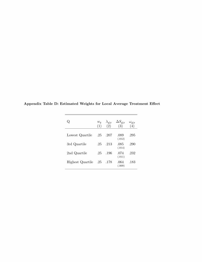
Appendix Table D: Estimated Weights for Local Average Treatment Effect

Q wq λq|x ∆Sq|x ωq|x(1) (2) (3) (4)

Lowest Quartile .25 .207 .089 .295(.012)

3rd Quartile .25 .213 .085 .290(.014)

2nd Quartile .25 .196 .074 .232(.011)

Highest Quartile .25 .178 .064 .183(.009)

46