The effects of liquidity regulation on bank assets and liabilities · 2016-06-01 · The Eﬀects...

The Effects of Liquidity Regulation onBank Assets and Liabilities∗

Patty Duijma and Peter Wiertsa,b

aDe Nederlandsche BankbVU University

Under Basel III rules, banks became subject to a liquiditycoverage ratio (LCR) from 2015 onward, to promote short-term resilience. Investigating the effects of such liquidity reg-ulation on bank balance sheets, we find (i) cointegration ofliquid assets and liabilities, to maintain a minimum short-termliquidity buffer; and (ii) that adjustment in the liquidity ratiois skewed towards the liability side. This finding contrasts withestablished wisdom that compliance with the LCR is mainlydriven by changes in liquid assets. Moreover, microprudentialregulation has not prevented a procyclical liquidity cycle insecured financing that is strongly correlated with leverage.

JEL Codes: E44, G21, G28.

1. Introduction

The Basel Committee on Banking Supervision (BCBS) has intro-duced a liquidity coverage ratio (LCR) from 2015 onward. It requiresbanks to hold a sufficient level of high-quality liquid assets againstexpected net liquid outflows over a thirty-day stress period, to pro-mote short-term resilience (BCBS 2009). The introduction of theLCR was motivated by the liquidity crisis of 2007–8, which occurredin combination with a solvency crisis. In this context, our contribu-tion addresses two questions: (i) what is the impact of a liquidityconstraint such as the LCR on individual bank behavior? and (ii)

∗We thank, without implicating them, Clemens Bonner, Jan Willem vanden End, Jon Frost, Leo de Haan, Dirk Schoenmaker, Robert Vermeulen, andJohn Williams for their helpful comments. The usual disclaimer applies. Authore-mails: [email protected] and [email protected].

385

386 International Journal of Central Banking June 2016

what has been the role of liquidity regulation before, during, andafter the liquidity and solvency crisis of 2007–8?

We study these questions by using a unique database for Dutchbanks, which have been subject to liquidity regulation that is compa-rable to Basel III’s LCR since 2003. We can systematically track liq-uid assets, liabilities, and their ratio during the upswing and down-swing of the financial cycle. Moreover, to investigate the link betweenliquidity and capital regulation, we collected bank-level informationon (core) capital, assets, and risk weights.

On the first question—i.e., the impact of the LCR on bankbehavior—several studies assume that the causality runs from lia-bilities to assets. These studies find that banks adjust their assets inresponse to a negative funding shock (Berrospide 2012; De Haan andvan den End 2013a, 2013b). An innovative element in our study isthat we let the data determine the direction of causality. We arguethat a constraint on the ratio between liquid assets and requiredliquidity implies that the two variables should be cointegrated, whichis supported by our findings. The error-correction regressions indi-cate that banks adjust their liabilities—and to a lesser extent theirliquid assets—when the LCR is above its equilibrium value, whilethe adjustment is even more skewed towards the liability side whenthe LCR is below its equilibrium value. In line with this finding, wefind that wholesale funding (with a high run-off rate in the denomi-nator of the LCR) has been replaced by more stable deposits duringthe aftermath of the crisis.

To address the second question—i.e., the role of liquidityregulation—we take a macroprudential perspective and investigateaggregate patterns in our variables before, during, and after thecrisis. Results indicate a strong increase in the levels of availableand required liquidity (the constituent parts of the LCR) before thefinancial crisis and a strong decrease afterwards. This cycle in short-term assets and liabilities occurs mostly through secured financing.It is accompanied by increasing leverage during the upturn anddecreasing leverage during the downturn. This is in line with earlierresults for the United States on the link between liquidity and lever-age (Adrian and Shin 2010). Moreover, the LCR itself is stronglycorrelated with the leverage ratio and shows a procyclical pattern.During increased risk taking in the upturn of the financial cycle,“cheaper” short-term wholesale funding (with a high run-off rate in

Vol. 12 No. 2 The Effects of Liquidity Regulation 387

the denominator of the LCR) is used to finance riskier and moreprofitable liquid assets (with a lower liquidity weight in the numera-tor), so that the LCR deteriorates. It is followed by de-risking and anincrease in the LCR during the subsequent downturn. This findingof procyclicality implies that banks’ short-term liquidity buffers areat their lowest point when the crisis starts, exactly when they areneeded the most. At the same time, regulatory risk-weighted capitalrequirements have not been a binding constraint, partly due to theprocyclicality of risk weights.

The rest of this paper is organized as follows. Section 2 presentsour conceptual framework. Section 3 provides the estimation resultson bank behavior under a liquidity constraint. Section 4 investigatesaggregate patterns for liquidity and solvency. Section 5 concludes.

2. Conceptual Framework

The LCR is defined as a ratio with the numerator representing theamount of “high-quality liquid assets” (HQLA), i.e., assets that canbe easily and immediately converted into cash at little or no loss ofvalue (Bank for International Settlements 2013). Liquid assets pri-marily consist of cash, central bank reserves, and, to a certain extent,marketable securities, sovereign debt, and central bank debt.1 Thedenominator is the net cash outflow within thirty days, which is thedifference between outgoing and incoming cash flows.

The LCR is defined as

LCR =High Quality Liquid Assets

Cash outflows − Cash inflows, (1)

where the cash outflows are subject to prescribed run-off rates andthe cash inflows are subject to prescribed haircuts in order to assign

1There are two categories of assets that can be included in the stock of HQLA:level 1 assets can be included without a limit, while level 2 assets can only com-prise up to 40 percent of the stock. Level 1 assets are limited to cash, centralbank reserves, and marketable securities representing claims on or guaranteedby, e.g., sovereigns, central banks, and the BIS (with a 0 percent risk weightunder the standardized approach for credit risk). Sovereign or central bank debtcan, under certain conditions (BIS 2013), also be reported as level 1 assets. Level2 assets consist of other marketable securities, corporate debt securities, and cov-ered bonds that satisfy certain conditions. See BIS (2013) for a comprehensivedefinition of HQLA.


these items a liquidity weight. The similarity between Basel IIIand the existing Dutch supervisory framework makes it possible toconstruct a comparable measure for the LCR; the Dutch liquiditycoverage ratio (DLCR).

In line with previous studies (e.g., Bonner 2012; De Haan andvan den End 2013a), the DLCR is defined as

DLCRi,t =ALi,t

RLi,t=

Σjaj · Asseti,j,t + Σkbk · Inflowi,k,t

Σlcl · Liabilityi,l,t + Σmdm · Outflowi,m,t,

(2)

where ALi,t and RLi,t stand for, respectively, available liquidity andrequired liquidity of bank i at time t. The variables aj , bk, cl, anddm represent the regulatory weights for the assets j, cash inflows k,liabilities l, and cash outflows m. Hence, available liquidity is definedas the weighted stock of liquid assets plus the weighted cash inflowsscheduled within the coming month. The liquidity weight on assetsis defined as 100 minus the haircut. These haircuts are determinedby the supervisor and aim to reflect the lack of market liquidity intimes of stress. Required liquidity is defined as the weighted stockof liquid liabilities plus the weighted cash outflows scheduled withinthe coming month. The liquidity weight on liabilities is defined asthe run-off rate. These run-off rates aim to reflect the probability ofwithdrawal and hence the funding liquidity risk.

The LCR and the DLCR reflect the same regulatory philosophyand are very similar. The main differences are the regulatory weights.In particular, the stock of HQLA is more narrowly defined for theLCR than for the DLCR. For the latter, the haircuts and run-offrates were determined by the Dutch regulator under the “Liquid-ity Regulation under the Wft,” for the first time in January 2003.2

There has been one structural change during the period under con-sideration. In May 2011, the Dutch Central Bank supplemented itsexisting rules with the “Liquidity Regulation under the Wft 2011.”3

2Wft stands for “Wet op het financieel toezicht,” the Dutch Financial Super-vision Act.

3The main change is a narrower definition of liquid assets; specifically, thehaircuts for debt instruments issued by credit institutions and other institutions(e.g., corporate bonds) have been increased due to the perceived illiquidity ofthese assets under stressed markets. At the same time, the run-off rate for


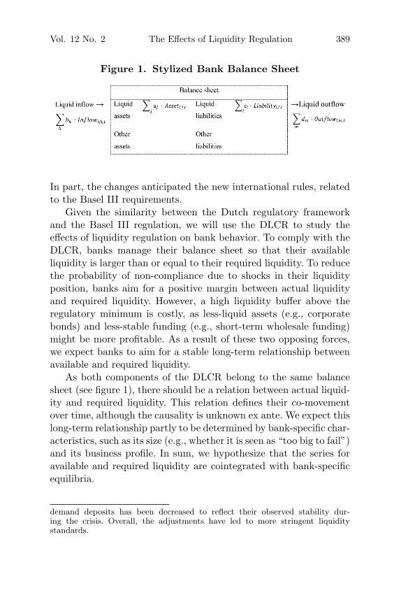
Figure 1. Stylized Bank Balance Sheet

In part, the changes anticipated the new international rules, relatedto the Basel III requirements.

Given the similarity between the Dutch regulatory frameworkand the Basel III regulation, we will use the DLCR to study theeffects of liquidity regulation on bank behavior. To comply with theDLCR, banks manage their balance sheet so that their availableliquidity is larger than or equal to their required liquidity. To reducethe probability of non-compliance due to shocks in their liquidityposition, banks aim for a positive margin between actual liquidityand required liquidity. However, a high liquidity buffer above theregulatory minimum is costly, as less-liquid assets (e.g., corporatebonds) and less-stable funding (e.g., short-term wholesale funding)might be more profitable. As a result of these two opposing forces,we expect banks to aim for a stable long-term relationship betweenavailable and required liquidity.

As both components of the DLCR belong to the same balancesheet (see figure 1), there should be a relation between actual liquid-ity and required liquidity. This relation defines their co-movementover time, although the causality is unknown ex ante. We expect thislong-term relationship partly to be determined by bank-specific char-acteristics, such as its size (e.g., whether it is seen as “too big to fail”)and its business profile. In sum, we hypothesize that the series foravailable and required liquidity are cointegrated with bank-specificequilibria.

demand deposits has been decreased to reflect their observed stability dur-ing the crisis. Overall, the adjustments have led to more stringent liquiditystandards.


3. Estimation Results

3.1 Unit-Root Tests and Cointegration

To test this hypothesis, we use monthly data from the Dutch super-visory liquidity report over the period July 2003 until April 2013.The report includes detailed information on liquid assets and liquidliabilities at an individual bank level for all banks subject to theliquidity regulation. We use data for fifty-nine banks for which thereported data are complete for the whole period under considera-tion.4 Ideally our data set would have been long enough to coverseveral financial cycles; however, it gives us some comfort that ourdata set covers at least the upswing and downswing of one financialcycle.

The long-run relationship between actual liquidity and requiredliquidity can only be estimated if the series are non-stationary andintegrated at the same order. Given the expected heterogeneity inbank behavior, we use a panel unit-root test that allows for differentindividual fixed effects in the intercepts and slopes of the cointegra-tion equation. Out of the full sample of fifty-nine banks, the seriesactual liquidity and required liquidity are both integrated at order1 for forty-one banks (see tables 1 and 2). Hence, we test for cointe-gration only for those banks. The results in table 3 indeed stronglyreject the null hypothesis of no cointegration against the alternativeof cointegration for each individual bank.5

3.2 Error-Correction Model

Given the finding of cointegration at the individual bank level, thelong-run equilibrium relationship can be estimated by fully modi-fied ordinary least squares (FMOLS) for heterogeneous cointegrated

4The underlying data are confidential. Where we show estimation results forindividual banks, we number them randomly so that results cannot be traced backto actual banks. Moreover, we only show aggregate data or estimation results andnot the underlying data.

5We use Pedroni’s (2001) cointegration test, since it allows for cross-sectionalinterdependence with different individual effects in the intercepts and slopes ofthe cointegration equation (i.e., a bank-specific long-run equilibrium).


Tab

le1.

Pan

elU

nit-R

oot

Tes

t

Thi

sta

ble

show

sth

ere

sult

sof

the

pane

lun

it-r

oot

test

base

don

the

Im-P

esar

an-S

hin

(IP

S)m

etho

d,w

here

the

null

hypot

hesi

sis

that

ofa

unit

root

.T

heap

prop

riat

enu

mber

ofla

gsis

sele

cted

bySc

hwar

zin

form

atio

ncr

iter

ion

(SIC

).T

hep-

valu

esar

esh

own

inpa

rent

hese

s.**

*de

note

sth

e1

per

cent

sign

ifica

nce

leve

l.B

ased

onth

ere

sult

sfo

rth

efu

llsa

mpl

e,th

eda

tase

tis

limit

edto

bank

sw

ith

tim

ese

ries

that

are

inte

grat

edat

orde

r1.

The

deci

sion

for

excl

usio

nis

mad

eba

sed

onth

epr

esen

ceof

aun

itro

otat

the

5per

cent

sign

ifica

nce

leve

l(s

eeta

ble

2).

Act

ual

Liq

uid

ity

Req

uir

edLiq

uid

ity

Lev

elFir

stD

iffer

ence

sLev

elFir

stD

iffer

ence

s

Full

Sam

ple

(Fifty

-Nin

eBan

ks)

#O

bs.

6,80

86,

766

6,78

86,

731

Tes

tSt

atis

tic

−6.

653

−88

.193

−9.

522

−92

.021

(0.0

00)∗

∗∗(0

.000

)∗∗∗

(0.0

00)∗

∗∗(0

.000

)∗∗∗

Lim

ited

Sam

ple

(For

ty-O

neBan

ks)

#O

bs.

4,72

24,

710

4,70

34,

691

Tes

tSt

atis

tic

−0.

657

−72

.827

1.07

6−

77.2

39(0

.256

)(0

.000

)∗∗∗

(0.8

59)

(0.0

00)∗

∗∗


Tab

le2.

Inte

rmed

iate

Unit-R

oot

Res

ults

Thi

sta

ble

show

sth

ein

divi

dual

augm

ente

dD

icke

y-Fu

ller

(AD

F)

test

resu

lts

for

all

indi

vidu

alti

me

seri

es.

The

null

hypot

hesi

sof

aun

itro

ot(n

on-s

tati

onar

ity)

iste

sted

agai

nst

the

alte

rnat

ive

that

ther

eis

noun

itro

ot.T

here

sult

sin

tabl

e1

show

that

the

null

hypot

hesi

sca

nnot

be

reje

cted

for

allfif

ty-n

ine

seri

es.H

owev

er,th

ein

term

edia

teA

DF

resu

lts

indi

cate

that

mos

tof

the

seri

essu

gges

tno

n-st

atio

nari

ty,m

eani

ngth

atth

ese

ries

are

inte

grat

edat

orde

r1

for

fort

y-on

eba

nks.

The

appr

opri

ate

num

ber

ofla

gsis

sele

cted

bySI

C.*,

**,an

d**

*de

note

10per

cent

,5

per

cent

,an

d1

per

cent

sign

ifica

nce

leve

ls,re

spec

tive

ly.

Act

ual

Liq

uid

ity

Req

uir

edLiq

uid

ity

Ava

ilab

leLiq

uid

ity

Req

uir

edLiq

uid

ity

Ban

kP

robab

ility

Lag

Pro

bab

ility

Lag

Ban

kP

robab

ility

Lag

Pro

bab

ility

Lag

10.

440

0.46

016

0.09

00.

03∗∗

22

0.58

00.

992

170.

542

0.99

43

0.07

30.

655

180.

999

0.85

24

0.79

00.

810

190.

302

0.35

05

0.00

∗∗∗

10.

00∗∗

∗2

200.

00∗∗

∗0

0.02

∗∗1

60.

193

0.33

321

0.68

00.

725

70.

291

0.81

722

0.00

∗∗∗

00.

00∗∗

∗0

80.

990

1.00

223

0.16

60.

0511

90.

402

0.64

224

0.00

∗∗∗

00.

00∗∗

∗0

100.

280

0.06

∗0

250.

121

0.71

111

0.24

20.

132

260.

300

0.30

012

0.38

40.

514

270.

434

0.24

213

0.61

00.

550

280.

351

0.19

214

0.57

30.

823

290.

762

0.00

∗∗∗

615

0.00

∗∗∗

00.

00∗∗

∗0

300.

01∗∗

20.

04∗∗

2

(con

tinu

ed)


Tab

le2.

(Con

tinued

)

Act

ual

Liq

uid

ity

Req

uir

edLiq

uid

ity

Ava

ilab

leLiq

uid

ity

Req

uir

edLiq

uid

ity

Ban

kP

robab

ility

Lag

Pro

bab

ility

Lag

Ban

kP

robab

ility

Lag

Pro

bab

ility

Lag

310.

621

0.00

∗∗∗

046

0.01

∗∗0

0.47

232

0.85

00.

335

470.

8912

0.00

∗∗∗

033

0.25

00.

190

480.

592

0.19

134

0.36

20.

582

490.

00∗∗

∗0

0.00

∗∗∗

035

0.33

10.

512

500.

311

0.75

136

0.29

20.

362

510.

460

0.03

∗∗2

370.

00∗∗

∗0

0.00

∗∗∗

052

0.48

20.

772

380.

270

0.39

053

0.28

10.

05∗∗

139

0.34

50.

325

540.

120

0.12

140

0.07

∗1

0.07

∗1

550.

03∗∗

10.

281

410.

301

0.87

156

0.00

∗∗∗

00.

00∗∗

∗0

420.

621

0.64

157

0.34

30.

482

430.

296

0.54

458

0.94

20.

863

440.

342

0.39

259

0.63

10.

182

450.

00∗∗

∗0

0.11

2


Tab

le3.

Coi

nte

grat

ion

Tes

tR

esults

Thi

sta

ble

show

sth

ere

sult

sof

Ped

roni

’sco

inte

grat

ion

test

.T

henu

llhy

pot

hesi

sof

noco

inte

grat

ion

iste

sted

agai

nst

the

alte

rnat

ive

that

aco

inte

grat

ing

vect

orex

ists

for

each

indi

vidu

alba

nk.T

heta

ble

show

spa

nelst

atis

tics

(lef

tco

lum

n)an

dgr

oup

stat

isti

cs(r

ight

colu

mn)

.T

heap

prop

riat

enu

mber

ofla

gsfo

rea

chin

divi

dual

tim

ese

ries

isse

lect

edby

SIC

.p-

valu

esar

ein

pare

nthe

ses.

***

deno

tes

the

1per

cent

sign

ifica

nce

leve

l.

Wit

hin

Dim

ensi

onB

etw

een

Dim

ensi

on

Pan

elv-

Stat

isti

c9.

764∗

∗∗(0

.000

)G

roup

rho-

Stat

isti

c−

33.8

45∗∗

∗(0

.000

)Pan

elrh

o-St

atis

tic

−14

.877

∗∗∗

(0.0

00)

Gro

upP

P-S

tati

stic

−20

.493

∗∗∗

(0.0

00)

Pan

elP

P-S

tati

stic

−10

.809

∗∗∗

(0.0

00)

Gro

upA

DF-S

tati

stic

−11

.473

∗∗∗

(0.0

00)

Pan

elA

DF-S

tati

stic

−10

.781

∗∗∗

(0.0

00)

Note

s:T

hepa

nel-st

atis

tics

appr

oach

poo

lsov

erth

e“w

ithi

n”di

men

sion

.Itte

ststh

enu

llhy

pot

hesi

sth

atth

efir

st-o

rder

auto

regr

essi

veco

effici

ent

onth

ere

sidu

als

isth

esa

me

for

each

indi

vidu

alba

nk.T

hegr

oup-

stat

isti

csap

proa

chpoo

lsov

erth

e“b

etw

een”

dim

ensi

on.

Ital

low

sth

eau

tore

gres

sive

coeffi

cien

tto

differ

for

each

indi

vidu

al.


panels. The bank-specific long-run equilibrium relationship betweenactual liquidity and required liquidity is given by

ALi,t = αALi + βAL

i,FMOLSRLi,t + εi,t, (3)

where αALi represents the individual fixed effects, and βAL

i,FMOLS isthe FMOLS estimator correcting for heterogeneity and serial corre-lation by adjusting the initial OLS estimator.

The lagged residuals from equation (3) define the error-correctionterms (ECT) in the following vector error-correction model:

ΔALi,t = αALi + ρALECTAL

i,t−1 + γiΔRLi,t−1 + uALi,t , (4)

where αALi represents the individual fixed effects, ΔALi,t represents

the level change of actual liquidity from time t − 1 to time t, andρAL represents the error-correction speed of adjustment of actualliquidity. ΔRLi,t−1 is included to control for short-term adjustments,and uAL

i,t is the error term. The same approach can be applied forrequired liquidity.6 To check for convergence to the long-run equi-librium, the estimated speed-of-adjustment coefficient should showa negative sign. This so-called Engle and Granger (1987) two-stepprocedure is applied to make inferences about the direction of causal-ity. Under this model, long-run causality is revealed by the statisticalsignificance of the adjustment coefficient ρAL.

The results are shown in the first row of table 4. These implythat when a bank moves away from its long-run equilibrium, itadjusts both assets and liabilities, and that the adjustment is skewedtoward the liability side of the balance sheet. That is, as the liquiditybuffer is above (below) equilibrium, banks decrease (increase) theiravailable liquidity and increase (decrease) their required liquidity.The estimated coefficient of –0.098 for available liquidity indicatesthat, after a shock to the long-run equilibrium, about 10 percentof this disequilibrium is corrected within one month through anadjustment in liquid assets. Likewise, the estimated coefficient of–0.221 for required liquidity indicates that about 22 percent of thisdisequilibrium is corrected within one month through an adjust-ment in liabilities. Given that required liquidity is determined by

6Then equations (3) and (4) will be replaced by, respectively, RLi,t =αRL

i +βRLi,FMOLSALi,t+εi,t and ΔRLi,t = αRL

i +ρRLECT RLi,t−1+γiΔALi,t−1+uRL

i,t .


Tab

le4.

(Asy

mm

etri

c)A

dju

stm

ent

Coeffi

cien

ts

Thi

sta

ble

show

sth

eer

ror-

corr

ecti

onte

rms

from

the

gene

raliz

edle

ast

squa

res

(GLS)

resu

lts

for

the

(thr

esho

ld)

erro

r-co

rrec

tion

mod

elfo

rfo

rty-

one

bank

sov

erth

eper

iod

July

2003

–Apr

il20

13(4

,749

obse

rvat

ions

).T

hehe

tero

sked

asti

city

ofth

eer

ror

term

sis

corr

ecte

dby

usin

gW

hite

robu

stst

anda

rder

rors

,an

dth

est

anda

rdde

viat

ions

are

disp

laye

din

pare

nthe

ses.

Cro

ss-s

ecti

onw

eigh

tsar

eus

ed,an

d**

and

***

deno

te5

per

cent

and

1per

cent

sign

ifica

nce

leve

ls,re

spec

tive

ly.

Dep

enden

tD

epen

den

tV

aria

ble

Var

iable

Sym

met

ric

ΔA

Lρ

AL

−0.

098∗

∗∗Δ

RL

ρR

L−

0.22

1∗∗∗

(0.0

11)

(0.0

24)

Asy

mm

etri

cΔ

AL

ρA

Lbelo

w−

0.05

9∗∗

ΔR

Lρ

RL

belo

w−

0.31

4∗∗∗

(0.0

22)

(0.0

26)

ΔA

Lρ

AL

above

−0.

129∗

∗∗Δ

RL

ρR

La

bove

−0.

142∗

∗∗

(0.0

21)

(0.0

29)


the weighted liabilities and cash outflows, the results indicate thatbanks adjust their funding mix—and to a lesser extent their portfolioallocation—when their liquidity position has changed.

A drawback of this first model is that it does not allow for asym-metric adjustment, i.e., it does not distinguish situations in whichthe liquidity buffer is above and below average. Banks may needto adjust more strongly when their DLCR falls below its long-runequilibrium and approaches the regulatory minimum. To allow forthis asymmetry, two dummy variables are introduced:

IALi,t =

{1 if ECTAL

i,t−1 < 0

0 if ECTALi,t−1 ≥ 0

IRLi,t =

{1 if ECTRL

i,t−1 ≥ 0

0 if ECTRLi,t−1 < 0.

(5)

The asymmetric error-correction model is estimated by

ΔALi,t = αALi + IAL

i,t ρALbelowECTAL

i,t−1 + (1 − IALi,t )ρAL

aboveECTALi,t−1

+ γALi ΔRLi,t−1 + vAL

i,t (6)

ΔRLi,t = αRLi + IRL

i,t ρRLbelowECTRL

i,t−1 + (1 − IRLi,t )ρRL

aboveECTRLi,t−1

+ γRLi ΔALi,t−1 + vRL

i,t , (7)

where ρALbelow(ρAL

above) and ρRLbelow(ρRL

above) represent the error-correction speed-of-adjustment coefficients given that a bank isbelow (above) its average liquidity level.

The results in the second row of table 4 suggest that the adjust-ment on the liability side becomes stronger when the DLCR is belowits equilibrium. On average, 31 percent of the deviation from thelong-run equilibrium is corrected within one month by a decrease inrequired liquidity. At the same time, adjustment on the asset sidebecomes slightly weaker and less significant, with only a 6 percentchange in available liquidity. When shocks move the DLCR aboveits long-run equilibrium, banks decrease liquid assets and increaseshort-term liabilities. On average, shifts in liquid assets and liabili-ties both correct approximately 13–14 percent of the deviation fromthe long-run equilibrium.


3.3 Robustness Check

As indicated already, regulatory changes to the DLCR were intro-duced in May 2011. As this may lead to a structural break, and inorder to exclude anticipation effects, we rerun the estimations for theperiod up to end-2010. Table 5 presents the results. The outcomesindicate an even stronger adjustment toward the liability side of thebalance sheet.

3.4 Discussion of Results

Our estimations indicate that a regulatory liquidity constraint influ-ences bank behavior, and that Dutch banks primarily adjust theirfunding mix when their DLCR falls below its long-run equilibrium.This section briefly compares our results with the academic litera-ture on the effects of liquidity regulation on bank behavior.7

Several authors investigate the effects of liquidity regulation onbanks’ liquid assets. De Haan and van den End (2013a) examinethe liquidity management of Dutch banks. They model the stock ofliquid assets as a function of the stock of liquid liabilities and thefuture cash inflows and outflows. A key finding is that banks keepliquid assets as a buffer against both the stock of liquid liabilitiesand net cash outflows. In another study, De Haan and van den End(2013b) find that in response to negative funding liquidity shocks,Dutch banks reduce wholesale lending, hoard liquidity in the formof liquid bonds and central bank reserves, and conduct fire sales of

7To save space, we focus only on studies based on econometric evidence, as itis closest to ours. In addition, there is a literature on the wider economic effectsof liquidity regulation, which also focuses mainly on the asset side. Examples areKing (2010), Perotti and Suarez (2010), and Wagner (2013). Other studies high-light that the LCR may provide incentives for increased reliance on central bankfunding; these studies include Ayadi, Arbak, and De Groen (2012), EuropeanBanking Authority (2012), and Coeure (2013). However, the data discussed insection 4 indicate that the reliance on central bank funding is limited for Dutchbanks. Toward the end of the observation period, claims on the central bankincrease markedly and outweigh reliance on central bank funding. This is con-sistent with the argument that the Netherlands was seen as a safe haven duringthe sovereign crisis of 2011–12. A possible effect of liquidity regulation on centralbank funding could therefore better be studied in countries where the reliance oncentral bank funding is higher.


Tab

le5.

Rob

ust

nes

sC

hec

k

Thi

sta

ble

show

sth

ege

nera

lized

leas

tsq

uare

s(G

LS)

resu

lts

for

the

(thr

esho

ld)

erro

r-co

rrec

tion

mod

elfo

rfo

rty-

one

bank

sov

erth

eper

iod

July

2003

–Dec

ember

2010

(3,6

49ob

serv

atio

ns).

The

hete

rosk

edas

tici

tyof

the

erro

rte

rms

isco

rrec

ted

byus

ing

Whi

tero

bust

stan

dard

erro

rs,an

dth

est

anda

rdde

viat

ions

are

disp

laye

din

pare

nthe

ses.

Cro

ss-s

ecti

onw

eigh

tsar

eus

ed,an

d**

and

***

deno

te5

per

cent

and

1per

cent

sign

ifica

nce

leve

ls,re

spec

tive

ly.

Dep

enden

tD

epen

den

tV

aria

ble

Var

iable

Sym

met

ric

ΔA

Lρ

AL

−0.

106∗

∗∗Δ

RL

ρR

L−

0.29

2∗∗∗

(0.0

14)

(0.0

20)

Asy

mm

etri

cΔ

AL

ρA

Lbelo

w−

0.09

5∗∗

ΔR

Lρ

RL

belo

w−

0.35

7∗∗∗

(0.0

25)

(0.0

36)

ΔA

Lρ

AL

above

−0.

119∗

∗∗Δ

RL

ρR

La

bove

−0.

215∗

∗∗

(0.0

26)

(0.0

43)


securities, especially equities.8 Using data on U.S. commercial banks,Berrospide (2012) studies the behavior of banks’ liquid assets as afunction of banks’ size, their capital ratio, their unused commitmentratio, and their share of core deposits (as a proxy for the role ofstable sources of funding). The author finds that stable sources offunding, such as deposits and bank capital, are key determinants ofthe holdings of liquid assets.

Overall, the econometric approach in the aforementioned stud-ies relies on the assumption that banks adjust liquid assets inresponse to shifts in their funding profile. Hence, our finding thatadjustment can also take place on the liability side of the balancesheet complements the existing literature. More recently, Banerjeeand Mio (2014) point to the effects of liquidity regulation on bothassets and liabilities. Their study is closest to our approach. Theyfind that banks that became subject to liquidity regulation signifi-cantly increased their share of HQLA. At the same time, banks alsoincreased their share of domestic retail deposits, offset by a similarreduction in short-term wholesale funding and non-resident deposits.The main difference with our paper is that we study the adjustmentto liquidity shocks after the regulation has been put in place, andwe rely on cointegration instead of causal regressions.

4. Aggregate Data

4.1 Patterns around the Crisis

We now turn to the second question on the role of liquidity regu-lation before, during, and after the liquidity and solvency crisis of2007–8. To do so, we shift focus from bank-level data toward aggre-gate patterns in the data for the Dutch banking sector as a whole.Figure 2 shows the average level of the DLCR for all banks in thesample and its development over time.

At the aggregate level, available liquidity always lies aboverequired liquidity, so that the DLCR requirement is respected and

8The authors suggest that the positive relation between equity holdings andsecured funding could also reflect the use of equities in repos and securities lend-ing transactions. When these activities are buoyant, banks’ equity holdings areuseful as collateral, while these become less useful when the secured fundingmarket collapses.


Figure 2. Dutch Liquidity Coverage Ratio (DLCR)and Its Components

Notes: The graph displays the aggregate level of liquidity of fifty-nine Dutchbanks for the period July 2003 until April 2013. The DLCR (left scale) isdefined as the ratio of available liquidity over required liquidity. The availableand required liquidity are given in billion euros (right scale) on a monthly basis.

minimum short-term liquidity buffers are maintained. As expected,available and required liquidity show strong co-movements, also atthe aggregate level. Both series increase strongly in the run-up tothe financial crisis, so that the aggregate balance expands strongly,and then decrease during the crisis. These large movements in avail-able and required liquidity mainly cancel out in the ratio, but notfully. In the run-up to the crisis, required liquidity increases some-what faster than available liquidity. As a result, the DLCR decreasesgradually towards the direction of the regulatory minimum ratio of1. During the crisis, required liquidity decreases more strongly thanavailable liquidity, so that the DLCR shows a substantial increase.This suggests a procyclical pattern of increased risk taking in theupswing of the financial cycle, i.e., a move toward “cheaper” whole-sale funding (with a high run-off rate in the denominator of theDLCR). It also suggests de-risking during the crisis, when wholesalefunding dries up and needs to be replaced by more stable fundingsources.

The aggregate data contradict established wisdom that changesin liquid assets are driving the liquidity ratio. On the contrary,the DLCR decreases in the run-up to the financial crisis, while


the amount of liquid assets increases. The DLCR then stronglyincreases during the crisis, while liquid assets fall. Finally, the datashow that the liquidity crisis of 2007–8, characterized by a strongoutflow of both liquid assets (decrease in available liquidity) andliabilities (decrease in required liquidity), is directly visible in theindividual series but not in the ratio, as it shows a substantialincrease.

Unfortunately, the data do not include the run-up to the intro-duction of the liquidity regulation. This is a limitation of our study:we cannot make inferences on a possible level shift in liquid assetsand liabilities due to the introduction of a binding liquidity ratio.9

However, we do observe data around the regulatory changes of May2011. Data show a fall in available liquidity, due to an increase inhaircuts, that leads to a drop in the DLCR. This is followed by agradual increase in the DLCR that is mostly driven by availableliquidity, toward a similar level to that observed during October2009–May 2011.

4.2 Balance Sheet Composition

Figures 3–6 provide an overview of the shifts in total assets andliabilities for the Dutch banking sector as a whole, and total assetsand liabilities weighted by their liquidity value (i.e., available andrequired liquidity). On the asset side, secured wholesale lending, con-sisting of (reverse) repos and securities lending, increases steadilyover 2003–7 and then declines strongly during the crisis. As securedwholesale lending is defined as highly liquid, it accounts for most ofthe dynamics in available liquidity. Likewise, on the liability side,the strongest dynamics are observed in secured wholesale funding,which mainly consists of repos. Moreover, over time, we observe ashift from wholesale funding toward retail demand deposits (with alow run-off rate). Overall, it appears that the liquidity componentsof the aggregate balance sheet reflect rapid balance sheet expan-sion and contraction over the financial cycle, driven by both securedfunding and lending.

9For the United Kingdom, Banerjee and Mio (2014) find that an increase inliquid assets has been one of the effects of the introduction of liquidity regulation.


Figure 3. Breakdown of Total Assets

Notes: This figure shows the aggregate asset allocation for the full sample offifty-nine banks over time, based on consolidated balance sheets. The order ofthe series is as follows, from bottom to top: secured wholesale lending, bonds,unsecured wholesale lending, claims on the CB, other (equity, cash, etc.), retaillending.

Figure 4. Breakdown of Available Liquidity(liquidity-weighted assets)

Notes: This figure shows the aggregate asset totals weighted by their liquidityvalue for the full sample of fifty-nine banks over time, based on consolidated bal-ance sheets. The order of the series is as follows, from bottom to top: securedwholesale lending, bonds, unsecured wholesale lending, claims on the CB, other(equity, cash, etc.), retail lending.


Figure 5. Breakdown of Total Liabilities

Notes: This figure shows the aggregate funding mix for the full sample of fifty-nine banks over time, based on consolidated balance sheets, including off-balance-sheet items (therefore total liabilities exceeds the total assets in figure 1). Theorder of the series is as follows, from bottom to top: secured wholesale fund-ing, other (CB borrowing, debt securities), fixed term deposits, off-balance-sheetitems, unsecured wholesale demand deposits, retail demand deposits.

Figure 6. Breakdown of Required Liquidity(liquidity-weighted liabilities)

Notes: This figure shows the aggregate liabilities weighted by their liquidityvalue for the full sample of fifty-nine banks over time, based on consolidated bal-ance sheets. The order of the series is as follows, from bottom to top: securedwholesale funding, other (CB borrowing, debt securities), fixed term deposits,off-balance-sheet items, unsecured wholesale demand deposits, retail demanddeposits.


4.3 Discussion of Results

From a microprudential perspective, the liquidity rules appear tohave been effective in the Dutch case, given that a minimum bufferof liquid assets has always been maintained to cover possible out-flows, as captured by required liquid assets. At the same time, theliquidity regulation did not prevent a procyclical liquidity cycle dri-ven by secured financing. Our findings therefore provide empiricalsupport to the “consensus view” on systemic liquidity risk (Acharya,Krishnamurthy, and Perotti 2011). According to this view, micro-prudential measures such as the LCR help support stability but arenot sufficient. First, they focus on individual liquidity risk but noton systemic liquidity risk. Second, they do not target liquidity risk inparticular in securities financing transactions and derivatives. Third,they are not countercyclical.

Several authors have already pointed to the relevance of securedfinancing—and repos in particular—in explaining the buildup ofrisk prior to the financial crisis in the United States, and contagionbetween institutions when this risk crystallized (e.g., Brunnermeierand Pederson 2009; Gorton and Metrick 2012; Copeland, Martin,and Walker 2014). Our results point to the relevance of securedfinancing for European countries such as the Netherlands. Futureresearch would be needed to provide further insights, especially onthe role played by the type of collateral (such as asset-backed securi-ties versus government bonds) and the pattern of margins and hair-cuts that may have been driving fire sales during the crisis, whichour data set unfortunately does not provide. Such research couldinform policy discussions on the use of through-the-cycle or coun-tercyclical margins and haircuts on securities financing transactions,as currently discussed in international forums such as the FinancialStability Board (FSB 2014).

A related approach points to the links between liquidity andleverage in the U.S. context. Adrian and Shin (2010) suggest thatfinancial market liquidity can be understood as the rate of growthof aggregate balance sheets. They argue that during the upswing ofthe financial cycle, asset prices increase so that capital increases andleverage falls.10 This provides an incentive to financial institutions

10Here leverage is defined as the ratio of total assets over capital.


to use this “excess capital” to maximize return on equity. They maytherefore extend their balance sheet through borrowing funds to pur-chase assets, so that capital falls (and leverage increases) back to itsprevious level. This translates into procyclical patterns in the size ofbanks’ balance sheets. For U.S. investment banks, Adrian and Shin(2010) present evidence for the expansion and contraction of balancesheets via repos (i.e., using purchased securities as collateral for thecash borrowing).11,12

To investigate such a possible link between liquidity and leveragefor Dutch banks, and with risk-weighted capital requirements moregenerally, we complemented our data set with balance sheet data onrisk weights, total assets, and (core) capital.13 Based on the possiblelink between liquidity and leverage, we expect a correlation betweenthe cycle in available and required liquidity and the leverage ratio(defined here as equity over total assets). This occurs given that theseries for available and required liquidity reflect debt-financed bal-ance sheet expansion and contraction. All else equal (i.e., if equitywould be constant), such a pattern would reflect procyclical lever-age. This procyclical pattern of the leverage ratio is confirmed infigure 7, which also highlights the strong correlation of the leverageratio with the DLCR.

Given that liquidity problems often reflect underlying solvencyproblems (Admati and Hellwig 2013), a link between liquidity ratiosand risk-weighted capital ratios could also be expected. As shown infigure 8, the correlation is indeed positive but not as strong as for the

11The Dutch banking sector is dominated by the largest three banks and istherefore highly concentrated: the largest three banks account for around 75percent of the total assets. These banks are universal banks: they combine tradi-tional banking with a sizable presence in securities markets. Our aggregate resultstherefore partly reflect the presence of these large banks in securities markets.

12Similarly, Geanakoplos (2010) points to procyclical leverage driven by pro-cyclical margins and haircuts on collateral.

13The confidential data originates from the supervisory solvency reportingrequirement. In contrast to the monthly reporting of liquidity data, the solvencydata is reported quarterly. Besides that, and also in contrast to the liquidity datareporting, foreign branches with a parent company within the European Unionare exempted from reporting, since the Dutch regulator plays no role in solvencysupervision of these banks. Hence, data on both the solvency and liquidity posi-tion are available for thirty banks. However, these thirty banks still represent 90percent of the total Dutch banking sector, based on 2013:Q1 data and measuredby total assets.


Figure 7. Liquidity and Leverage Ratioa

Notes: This figure shows the weighted-average leverage ratio (left scale) andDLCR (right scale) for a sample of thirty banks on a quarterly basis for theperiod 2004:Q1–2013:Q1.aThe leverage ratio is defined as total tier 1 capital divided by total assets.

Figure 8. Liquidity and Capital Ratioa

Notes: This figure shows the weighted-average capital ratio (left scale) andDLCR (right scale) for a sample of thirty banks on a quarterly basis for theperiod 2004:Q1–2013:Q1.aThe capital ratio is defined as the total eligible capital divided by total risk-weighted assets (Basel definition).


Figure 9. Risk Weights

Notes: This figure shows the aggregate asset totals, risk-weighted assets, andthe implied average risk weights (right scale) on a quarterly basis for the period2004:Q1–2013:Q1.

leverage ratio. This difference can be explained by the procyclicalchange in average risk weights during our sample period (figure 9).As a result, risk-weighted capital requirements remained relativelystable above their regulatory minimum in the run-up to the crisis,despite increasing leverage. Further discussions on the performanceof risk weights as ex ante and ex post measures of risk are subjectto a separate literature, which is beyond the scope of this paper (seeLe Lesle and Avramova 2012).

Finally, our finding of a procyclical pattern in the DLCR is inline with Goodhart et al. (2012). These authors argue that banksnaturally have more liquid assets during booms than during busts,and that if a liquidity ratio is binding during a boom, it will beeven more restrictive during a bust, making it a procyclical regula-tory ratio. Therefore, the authors propose countercyclical haircuts(i.e., liquidity weights), so that the liquidity requirements becometime varying and the liquidity buffer can be released during timesof financial stress.

5. Conclusion

The main implication of our study is that banks adjust their liq-uid liabilities, and to a lesser extent their liquid assets, in responseto shocks in their liquidity positions. In the Dutch case, liquidity


regulation appears to have been effective from a microprudential per-spective but not from a macroprudential perspective. While banksrespect the minimum liquidity ratio, liquidity regulation has notprevented a procyclical liquidity cycle in short-term secured financ-ing that is strongly correlated with leverage. At the same time, theincrease in leverage was not visible in the regulatory capital ratios.Hence, monitoring the risk-weighted capital requirements, or theLCR as a ratio, does not necessarily signal the buildup or mate-rialization of aggregate risks. It may need to be complemented bymonitoring the LCR’s constituent parts, both at an institutionallevel and for the banking sector as a whole, and interpreted againstthe background of movements in balance sheet size and leverage.

Furthermore, and in line with previous research, our findingspoint to the significant role of secured financing for explaining theleverage and liquidity cycle. This calls for further research on therole played by the type of collateral, and the pattern of asset prices,margins, and haircuts that may have been driving the liquidity cycleand fire sales during the crisis.

References

Acharya, V., A. Krishnamurthy, and E. Perotti. 2011. “A ConsensusView on Liquidity Risk.” VoxEU.org, September 21.

Admati A., and M. Hellwig. 2013. The Bankers’ New Clothes:What’s Wrong with Banking and What to Do about It. Princeton,NJ: Princeton University Press.

Adrian, T., and H. S. Shin. 2010. “Liquidity and Leverage.” Journalof Financial Intermediation 19 (3): 418–37.

Ayadi, R., E. Arbak, and P. W. De Groen. 2012. “ImplementingBasel III in Europe: Diagnosis and Avenues for Improvement.”CEPS Policy Brief No. 275.

Banerjee, R., and H. Mio. 2014. “The Impact of Liquidity Regulationon Banks.” BIS Working Paper No. 470.

Bank for International Settlements. 2013. “Basel III: The LiquidityCoverage Ratio and Liquidity Risk Monitoring Tools.” (Janu-ary).

Basel Committee on Banking Supervision. 2009. “Strengthening theResilience of the Banking Sector.” Consultative Document.


Berrospide, J. 2012. “Liquidity Hoarding and the Financial Crisis:An Empirical Evaluation.” Manuscript, Board of Governors ofthe Federal Reserve System.

Bonner, C. 2012. “Liquidity Regulation, Funding Costs and Corpo-rate Lending.” DNB Working Paper No. 361.

Brunnermeier, M. K., and L. H. Pedersen. 2009. “Market Liquid-ity and Funding Liquidity.” Review of Financial Studies 22 (6):2201–38.

Coeure, B. 2013. “Liquidity Regulation and Monetary Policy Imple-mentation: From Theory to Practice.” Speech presented atToulouse School of Economics, Toulouse, October 3.

Copeland, A., A. Martin, and M. Walker. 2014. “Repo Runs: Evi-dence from the Tri-Party Repo Market.”Journal of Finance 69(6): 2343–80.

De Haan, L., and J. W. van den End. 2013a. “Bank Liquidity,the Maturity Ladder, and Regulation.” Journal of Banking andFinance 37 (10): 3930–50.

———. 2013b. “Banks’ Responses to Funding Liquidity Shocks:Lending Adjustment, Liquidity Hoarding and Fire Sales.” Jour-nal of International Financial Markets Institutions and Money26: 152–74.

Engle, R., and C. W. J. Granger. 1987. “Forecasting and Testing inCo-Integrated Systems.” Journal of Econometrics 35 (1): 143–59.

European Banking Authority Banking Stakeholder Group. 2012.“New Bank Liquidity Rules: Dangers Ahead.” EBA PositionPaper.

Financial Stability Board. 2014. “Strengthening Oversight and Reg-ulation of Shadow Banking: Regulatory Framework for Haircutson Non-Centrally Cleared Securities Financing Transactions.”(October).

Geanakoplos, J. 2010. “The Leverage Cycle.” In NBER Macroeco-nomics Annual 2009, Vol. 24, ed. D. Acemoglu, K. Rogoff, andM. Woodford, 1–65. University of Chicago Press.

Goodhart, C. A., A. K. Kashyap, D. P. Tsomocos, and A. P. Var-doulakis. 2012. “Financial Regulation in General Equilibrium.”NBER Working Paper No. 17909.

Gorton, G. B., and A. Metrick. 2012. “Who Ran on Repo?” NBERWorking Paper No. 18455.


King, M. R. 2010. “Mapping Capital and Liquidity Requirements toBank Lending Spreads.” BIS Policy Paper No. 324.

Le Lesle, V., and S. Avramova. 2012. “Revisiting Risk-WeightedAssets: Why Do RWAs Differ across Countries and What CanBe Done about It?” IMF Working Paper No. 12/90.

Pedroni, P. 2001. “Fully Modified OLS for Heterogeneous Cointe-grated Panels.” In Nonstationary Panels, Panel Cointegration,and Dynamic Panels, Vol. 15 of Advances in Econometrics Series,ed. B. H. Baltagi, T. B. Fomby, and R. C. Hill, 99–130. EmeraldGroup Publishing, Ltd.

Perotti, E., and J. Suarez. 2010. “Liquidity Risk Charges as a Pri-mary Macroprudential Tool.” Policy Paper No. 1, DuisenbergSchool of Finance.

Wagner, W. 2013. “Regulation Has to Come to Terms with theEndogenous Nature of Liquidity.” Policy Brief No. 24, Duisen-berg School of Finance.

The effects of liquidity regulation on bank assets and liabilities · 2016-06-01 · The Eﬀects...

Documents

Transcript of The effects of liquidity regulation on bank assets and liabilities · 2016-06-01 · The Eﬀects...