The Effects of Leverage on Stock Returns

Author: Matilda Andersson

September 2, 2016

Supervisor: Erik NorrmanBachelors Thesis

Lund UniversitySchool of Economics and Management

Department of Economics

Abstract

This paper investigates the relationship between capital structure and stock returnsfor Swedish firms listed on the Nasdaq OMX Stockholm Stock Exchange. Actualstock returns and leverage figures in form of total, long-term and short-term debtare used in the calculations. The results suggest, in contrast with a majority offundamental theories, that there is a negative relationship between leverage and stockreturns. The results indicate that investors are not being compensated for the extrarisk they are taking on when investing with high-leveraged firms. Several previousempirical studies has come to the same conclusion. This study in conjunction withother earlier empirical studies question a very common understanding of capitalstructure.

1

Contents

1 Introduction 5

1.1 Background . . . . . . . . . . . . . . . . . . . . . . . . . . . . . . . . 5

1.2 Purpose and Contribution . . . . . . . . . . . . . . . . . . . . . . . . 6

1.2.1 Research Questions . . . . . . . . . . . . . . . . . . . . . . . . 6

1.3 Limitations of the Study . . . . . . . . . . . . . . . . . . . . . . . . . 7

1.4 Disposition . . . . . . . . . . . . . . . . . . . . . . . . . . . . . . . . 7

2 Theoretical framework 9

2.1 Measurements of Capital Structure . . . . . . . . . . . . . . . . . . . 9

2.1.1 Capital Structure . . . . . . . . . . . . . . . . . . . . . . . . . 9

2.1.2 Leverage . . . . . . . . . . . . . . . . . . . . . . . . . . . . . . 9

2.2 Capital Structure in Theory . . . . . . . . . . . . . . . . . . . . . . . 10

2.2.1 Modigliani-Miller Theorem . . . . . . . . . . . . . . . . . . . 10

2.2.2 Agency Theory . . . . . . . . . . . . . . . . . . . . . . . . . . 11

2.2.3 Trade-off Theory . . . . . . . . . . . . . . . . . . . . . . . . . 11

2.2.4 Pecking Order Hypothesis . . . . . . . . . . . . . . . . . . . . 12

2.2.5 Market Timing Theory . . . . . . . . . . . . . . . . . . . . . . 13

2.3 Review of Empirical Studies . . . . . . . . . . . . . . . . . . . . . . . 13

2.3.1 Positive Relationship between Leverage & Stock Returns . . . 13

2.3.2 Negative Relationship between Leverage & Stock Returns . . 13

2.3.3 Pecking-order Hypothesis versus Trade-off Theory . . . . . . 14

2.3.4 Short- and Long-term Debt . . . . . . . . . . . . . . . . . . . 15

2.3.5 Industry Specifics of Capital Structure . . . . . . . . . . . . . 15

2.4 Hypotheses . . . . . . . . . . . . . . . . . . . . . . . . . . . . . . . . 15

2

3 Methodology 17

3.1 Research Approach . . . . . . . . . . . . . . . . . . . . . . . . . . . . 17

3.2 Data Collection . . . . . . . . . . . . . . . . . . . . . . . . . . . . . . 17

3.2.1 Data Selection . . . . . . . . . . . . . . . . . . . . . . . . . . 17

3.2.2 Data Loss . . . . . . . . . . . . . . . . . . . . . . . . . . . . . 20

3.3 Variables . . . . . . . . . . . . . . . . . . . . . . . . . . . . . . . . . . 21

3.3.1 Stock Returns . . . . . . . . . . . . . . . . . . . . . . . . . . . 21

3.3.2 Capital Structure . . . . . . . . . . . . . . . . . . . . . . . . . 21

3.3.3 Control Variables . . . . . . . . . . . . . . . . . . . . . . . . . 22

3.3.4 Industry Separation . . . . . . . . . . . . . . . . . . . . . . . 24

3.4 Regression Model . . . . . . . . . . . . . . . . . . . . . . . . . . . . . 24

3.4.1 Multiple Regression Model . . . . . . . . . . . . . . . . . . . . 24

3.4.2 Choice of Model for Panel Data . . . . . . . . . . . . . . . . . 25

3.4.3 Regression Specification . . . . . . . . . . . . . . . . . . . . . 26

3.4.4 Significance Level . . . . . . . . . . . . . . . . . . . . . . . . . 27

3.4.5 Validity Tests . . . . . . . . . . . . . . . . . . . . . . . . . . . 27

4 Empirical Findings 31

4.1 Descriptive Statistics . . . . . . . . . . . . . . . . . . . . . . . . . . . 31

4.2 Near Multicollinearity . . . . . . . . . . . . . . . . . . . . . . . . . . 32

4.3 Regression Results . . . . . . . . . . . . . . . . . . . . . . . . . . . . 33

4.3.1 Industrial Firms . . . . . . . . . . . . . . . . . . . . . . . . . 33

4.3.2 Technology Firms . . . . . . . . . . . . . . . . . . . . . . . . . 35

5 Analysis & Discussion 37

5.1 Stock Returns and Capital Structure . . . . . . . . . . . . . . . . . . 37

5.1.1 Total Debt Ratio . . . . . . . . . . . . . . . . . . . . . . . . . 37

3

5.1.2 Short-term and Long-term Debt Ratios . . . . . . . . . . . . 38

5.2 Industry . . . . . . . . . . . . . . . . . . . . . . . . . . . . . . . . . . 39

6 Conclusion 40

6.1 General Thoughts . . . . . . . . . . . . . . . . . . . . . . . . . . . . . 40

6.2 Limitations . . . . . . . . . . . . . . . . . . . . . . . . . . . . . . . . 40

6.3 Future Research . . . . . . . . . . . . . . . . . . . . . . . . . . . . . . 41

7 References 43

7.1 Books . . . . . . . . . . . . . . . . . . . . . . . . . . . . . . . . . . . 43

7.2 Online Journal Articles . . . . . . . . . . . . . . . . . . . . . . . . . . 43

7.3 Printed Journal Articles . . . . . . . . . . . . . . . . . . . . . . . . . 46

7.4 Websites . . . . . . . . . . . . . . . . . . . . . . . . . . . . . . . . . . 47

7.5 Databases . . . . . . . . . . . . . . . . . . . . . . . . . . . . . . . . . 47

4

1 Introduction

This introductory chapter aims to present the background of why capital structure hasbeen a researched subject and why it is still interesting today, to study the relationshipbetween a firm’s performance and its capital structure. It will include the purpose ofthe study, the main research questions and the limitations of the study. At the endan outline will be presented for the study.

1.1 Background

What defines a successful company? A company could be successful in many ways,in economical terms a company’s success however is often linked with the company’svalue creation, i.e. the ability of the company to generate future returns in termsof invested capital. The value of a firm is driven by earnings and growth (Koller& Goedhart 2010), which in turn are rooted in the firms business strategy, uniqueassets, management, strategic market position, among other things (Sparrow 2013).Economists, managers and investors have always been seeking identifiers of successand many firms specific variables has as a result been considered crucial indicatorsof a firms performance.

A feature that applies to all companies is that they need financing to operate theiractivities. Even the smallest most simple business needs capital. To maximise profitsit is in every company’s interest to raise capital as cheaply as possible. This taskis however not always easy since there are many different ways of raising capital.One way is to raise capital is by borrowing money from banks or bondholders,another is to sell ownership stakes by issuing equities. Still, many more optionsare available. Firms could for example issue hybrid securities in form of convertibledebt or preferred stocks (Financial Times). A firm’s composition of different typesof capital is denoted as the firm’s capital structure (Brealey, Myers & Allen 2011).

Since capital is a central component for conducting business and could be raised inso many different ways, capital structure has become a topic of discussion. Doesthe choice of capital structure matter for a firm’s profitability or returns? Whatcombination of capital lends itself to the greatest measure of success? In the attemptto generalise ideas of capital structure several theories of capital structure has beendeveloped. The first was the Modigliani & Miller theorem published in 1958 whichproposed that future stocks return should increase with the amount of debt. Theirreasoning behind the proposition was that the higher the proportion of debt in afirm, the higher the risk of owning the firm’s stock and the more should investorsbe compensated in terms of returns (Modigliani & Miller 1958). After Modigliani &Miller other theories such as the trade-off theory and the pecking order hypothesiswas developed.

Capital structure has since the late 1950’s been subject for many empirical studies.Interestingly enough the proposed relationship between firm performance and capitalstructure has not been conclusively proven (Baker & Martin 2001). Several studies

5

come to the conclusion that firm performance correlate positively with the proportionof debt, others find a negative relationship. It is in other words still unclear whethercapital structure affects a firm’s performance and success and if so in which way.

1.2 Purpose and Contribution

The purpose of this study is to investigate if a firm’s stock return can be explainedby its capital structure and if fundamental theories as well as previous empiricalfindings can be applied to firms listed on the Nasdaq OMX Stockholm Stock Ex-change. As mentioned above previous empirical studies have presented somewhatcontradictory results, some agreeing som disagreeing with the fundamental theoriesof capital structure. The conflicting results justifies further research and investi-gation. The purpose of this paper is to contribute to the body of research on thesubject. By focusing on Swedish data, on which few previous papers have beenwritten, the ambitions of the study is to stand out and be able to contribute.

Within the spectra of existing studies, few researchers have been focusing on marketbased measurements of firm performance such as stock returns. Instead many stud-ies have chosen to focus on book values such as return on equity or return on assetsas dependent variable. By basing the study on stock returns instead of book values,this paper will investigate the relationship between firms performance and capitalstructure from an investor’s perspective. The study will try to explore if investorsshould take capital structure into account in their investment decisions. Stock re-turns hasn’t (to my knowledge) been used before as a proxy for firm performance instudies based on Swedish data. The papers ambition is to fill this research gap.

Most studies that investigate the relationship between shareholders return and capi-tal structure use the Capital Asset Pricing Model (CAPM) to determine shareholderreturn and are using expected stock returns as dependent variable. By measuringactual stock returns this study will capture the actual effect of leverage on stockreturns, not the impact leverage has on future returns.

This study will be employing regression on panel data. Panel data consist of bothcross-sectional and time-series observations and is currently preferred to using cross-sectional or time-series data separately (Dougherty 2011). Since using panel datais quite a new method, older studies are rarely if ever based on panel data. Olderstudies may therefore be less accurate than newer ones.

1.2.1 Research Questions

The study will be built upon two research questions. The main research question isproposed as follows:

• How are stock returns affected by capital structure in Swedish listed firmsduring 2006-2015?

6

The secondary research question is:

• Does the observed relationship between capital structure and stock returnsvary between the industrial and the technology industry?

1.3 Limitations of the Study

The study is limited by focusing on Swedish firms listed on the Nasdaq OMX Stock-holm stock exchange. It is also limited to a ten-years time period (2006-2015). Usingstock returns limits the sample size since no observations for stock returns are avail-able before the point in time when the company in question is listed. To collectsufficiently large samples the lower limit is set to year 2006.

Only two industries will be investigated in this study: The industrial as well as thetechnology industry. The financial industry is excluded due to different regulationsregarding capital structure (Alves & Francisco 2014). Other industries are excludedbecause of a lack of data due to missing data.

1.4 Disposition

Chapter 1 IntroductionThe introducing chapter aims to present the background to and purpose of the study.It will further present the main research questions that are going to be investigatedand the limitations of the study.

Chapter 2 Theoretical frameworkThe theoretical framework will present main theories on capital structure as well asprevious empirical evidence of the relationship between stock return and leverage.The theories and empirical findings arrive as four hypotheses presented at the endof this chapter.

Chapter 3 MethodologyThis chapter aims to explain the steps taken and choices made along the processof this study. The chapter will for example explain choices made regarding dataselection, regression model and control variables.

Chapter 4 Empirical resultsIn this chapter descriptive statistics, correlation matrixes and the empirical resultsof the regressions will be presented.

Chapter 5 Analysis & DiscussionThe chapter Analysis & Discussion will contain analysis of the empirical result in thecontext of fundamental theories and previous empirical findings presented in chapter2. The purpose of the chapter is to resolve if the stated hypothesis shall be rejectedor not.

7

Chapter 6 ConclusionThe final chapter will summarise the results of the study. It will also reflect onlimitation of the study and purpose suggestions for further research on the subject.

8

2 Theoretical framework

This chapter will initially be introducing the concept of capital structure. After thatthe most fundamental theories on capital structure will be presented, followed byprevious empirical findings of the relationship between leverage and stock returns.The theories and the empirical evidence will be the basis for the hypotheses developedwhich are presented at the end of this chapter.

2.1 Measurements of Capital Structure

2.1.1 Capital Structure

Capital structure is at its simplest defined as the composition of debt and equityfinancing (Brealey, Myers & Allen 2011) and determines who has the claim of afirm’s assets and in what order. Investors provide equity financing while banks orbondholders provide financing trough debt. A firm’s capital structure may be moreor less complicated since there are options to issue also other types of securitiesfor financing, e.g. hybrid securities such as convertible debt and preferred stocks(Financial Times). The capital structure could be measured as the ratio of debtthrough equity or debt through total assets (Örtqvist 2006). A high debt to totalassets ratio implies that a firm raises more debt proportionally to issuing of equity,i.e. the firm is highly leveraged. It is important to note that the debt to total assetsratio could change both due to increased borrowing and to changes in the marketvaluation of equity (Brealey, Myers & Allen 2011).

2.1.2 Leverage

Leverage is a commonly used word for borrowed money that allows for increasedreturns, theoretically. Leverage is also used as a substitute for the proportion of debtthat is uitilised by the company in question for financing its assets, i.e. the debt ratio.The general idea of using the word leverage instead of debt ratio regarding a firm’scapital structure is to illustrate that more debt implies more risk. Equity is moresensitive to changes in firm value in a high-leveraged firm than in a low-leveragedone. A potential loss or gain will in other words be larger for a high-leveraged firmthan a low-leveraged firm. This is called the leverage effect. Leverage is often definedas the proportion of all of a firm’s liabilities, which among other things include long-term and short-term debt as well as pensions obligations (Brealey, Myers & Allen2011).

9

2.2 Capital Structure in Theory

2.2.1 Modigliani-Miller Theorem

The Modigliani-Miller theorem, developed in 1958 by Franco Modigliani and MertonH. Miller, has laid the foundation for many of todays capital structure theories andhas also been the subject of great many an empirical study (Baker & Martin 2011).The theory consists of two main propositions and is based on five perfect capitalmarket assumptions (Modigliani & Miller 1958):

• There is neither transaction costs nor taxes in capital markets and investorsare able to borrow at the same cost as companies

• There are no bankruptcy costs

• There is no asymmetric information in the capital markets, e.g the marketparticipants share similar expectations about earnings and volatility

• Market participants are not able to affect market prices

• A firm’s capital structure is constant and well known

Proposition I suggests that the market value of a firm is independent of its capitalstructure (Baker & Martin 2011):

Vj = (Sj +Dj) = X̄j (1)

Where:Vj = Market value of a firmSj = Market value of the firm’s common sharesDj = Market value of the firm’s debtX̄j = The present value of future expected returns on the firms assets

Proposition II which holds when proposition I holds, suggests that common stockreturns increase with the amount of debt. Proposition II is formulated as(Baker & Martin 2011):

ij = ρk + (ρk − r)Dj

Ej(2)

Where:ij = Expected return of a common stockρk = The capitalisation rate for the equity streamr = The cost of debt

Dj/Ej = The ratio between debt and equity

10

Modigliani and Miller argue in their 1958 paper that the higher the proportion ofdebt in a firm, the higher the risk of owning said firms stock. In order to compensateinvestors for the higher risk, stocks for highly leveraged firms should generate a higherreturn (Modigliani & Miller 1958).

Empirical studies have come to contradictory conclusions. Even though the firstproposition widely has been accepted theoretically it hasn’t been conclusively provento hold empirically (Miller 1988).

2.2.2 Agency Theory

In 1976 Jensen & Meckling published a study in which they tried to detail optimisinga firms capital structure. Their reasoning is built upon the principal agents theory, i.ethat agents are utility maximizing and therefore generally act in their own interestsinstead of the principals. Principals can in this case take control by incentivisingagents, however this generates costs, so called agency costs. The principal-agentrelationship fit the relationship of a stakeholder and a manager of a firm. Jensen &Meckling (1976) suggests that increasing the level of debt up to a certain level woulddecrease the agency costs since debt holders would get more power and control andthereby out-competing the agents potential egotistical actions. Thereby higher levelsof debt, up to a certain level, may improve a firm’s performance (Jensen & Meckling1976).

2.2.3 Trade-off Theory

Myers (1984) further developed the optimal capital structure choice, which laterbecame the trade-off theory. The trade-off theory suggests that managers view thecapital structure decision of their firms as a trade-off between interest tax shieldon the one side and costs of financial distress on the other. It also suggests thatcompanies with a large amount of safe assets, such as tangible assets, in combinationwith a high income will finance their activities with a great proportion of debt. Sincethe tax-shield, assets structure and income are firm specific there is an optimal debt-ratio for each company. The marginal utility of issuing additional debt decreaseswhen the debt proportion of total capital increases (Brealey, Myers & Allen 2011).As long as more debt is optimal, shareholders benefit from more debt (Baker &Martin 2011). The value of a firm is according to the trade-off theory formulated as(Brealey, Myers & Allen 2011):

V = Ve + PV (Tax Shield) − PV (Costs of Financial Distress) (3)

11

V = Firm ValueVe = Firm Value, if all Equity FinancedPV = Present Value

The trade-off theory explains why capital structure setups may differ between indus-tries. Since technological high-growth companies normally have a lot of risky assetsand a large amount of intangible assets, they often lack the opportunity to raisecheap debt. According to Brealey, Myers & Allen (2011) these firms often financetheir activities by a high proportion of equity in relation to debt.

2.2.4 Pecking Order Hypothesis

The pecking order hypothesis is based on the assumption that there is a degree ofinformation asymmetry between managers and investors. That is, the managersknow more about their companies value, risks and future than the investors. Aproof of this is that stock prices often rise after announcement of increased comingdividend payments. Asymmetric information has an impact also on a company’schoice of financing. Financing could be done internally or externally and by issuingeither debt or equity. The pecking order is that a firm at all times prefers internalfinancing to external and in cases when external financing is the only available optiondebt is preferred over equity. With the pecking order assumptions in mind, issuanceof equity is a last resort. Issuing equity would according to this theory send badsignals and investors may in such a scenario fear that the firm is in financial distress.That in turn would cause the stock price to dip (Brealey, Myers & Allen 2011).

Issuing equity will not necessarily affect the stock price negatively for all firms. High-tech, high-growth firms possessing large amounts of intangible assets rarely have theopportunity to raise debt. Due to high costs of debt and difficulties with generatingcash flows large enough for covering debt and interest rate payments, equity will bethe only financing option to achieve growth. Since this characterise all high-techhigh-growth firms the impact of the pecking order will not be as distinct as formature profitable firms. Profitable firms in general are expected to pay down debtas soon as they are able to (Brealey, Myers & Allen 2011).

According to the pecking order hypothesis there is no optimal proportion of debt.The theory just concludes that the optimal proportion of debt differ between differenttypes of firms. Profitable firms issue less equity and use less external financing thanhigh-growth firms (Brealey, Myers & Allen 2011). Hovakimian, Opler & Titman(2001) agree with the pecking-order hypothesis and similarly suggest that profitablefirms in general take advantage of high income and pay down debt.

12

2.2.5 Market Timing Theory

The market timing theory assumes that managers are sometimes irrational in theirbehaviour. In cases where a manager’s outlook regarding their own company ismore stable than the general investor’s, they may decide to (and likely will) issueequity when the stock price is high and raise debt in times when the stock price islow. Managers are in other words, due to asymmetric information, able to time themarket at least somewhat efficiently. The market timing theory as such suggests thatdebt could correlate negatively with stock returns (Brealey, Myers & Allen 2011).

According to Masulis & Korwar’s (1986) and Asquith and Mullin’s (1986) studies,firms generally issue more equity when the stock price goes up. Graham & Harvey’s(2001) survey additionally shows that the majority of asked CFOs say they havetimed the market when issuing equity. Similar evidence comes from Hovakimian,Hovakimian & Tehranian (2004) whom find the probability of issuing equity higherwhen the spot stock price is high.

2.3 Review of Empirical Studies

2.3.1 Positive Relationship between Leverage & Stock Returns

Hamada (1969) takes a theoretical approach to researching if Modigliani & Miller’ssecond proposition holds by investigating the effect of capital structure on systemicrisk of common stocks. His conclusion is that the rate of return increases with thedebt ratio. In a later study made in 1972 using data of U.S firms, he proves that histhesis holds and establishes that there is a positive correlation between leverage andstock returns (Baker & Martin 2011).

Masulis’s findings are in line with Hamada’s. In his 1983 study he investigates theimpact leverage changes have on stock returns. His results suggest that both firmvalue and changes in stock prices correlate positively with changes in the debt ratio(Masulis 1983).

Bhandari (1988) shows that expected common stock returns on a monthly basiscorrelate positively with annual debt-to-equity ratios. The relationship is observedboth regarding firms of all sectors as well as manufacturing firms (specifically).

2.3.2 Negative Relationship between Leverage & Stock Returns

Ardatti (1967) examines the relationship between leverage and the geometrical aver-age of returns for industrial, railroad and utilities firms. He finds a negative relation-ship between the variables, however it is statistically insignificant. Arditti concludesthat the insignificancy may be a result of omitting risk variables that relates posi-tively to return and negatively to leverage.

13

Hall &Weiss (1967) come across a negative relationship between leverage and returnswhen investigating the relationship between firm size and profitability. They probethe 500 largest industrial firms and define stock returns as returns on equity aftertaxes.

Adami et al. (2015) explore if there is any relationship between capital structureand stock performance during 1980 and 2008 for stocks listed on the London StockExchange. Their empirical results show that debt financing negatively affect stockreturns. The results are explained by investors preferring to invest in financiallyflexible firms and therefore generate higher returns when investing in low-leveragedfirms than high-leveraged firms (Adami et al 2015).

Penman, Richardson & Tuna’s (2007) conclusions are in line with Adami et al.’s;market leverage correlates negatively with stock returns. They suggest that theunexpected relationship appears due to some of the following reasons: 1) there aremeasurement errors in the leverage figures, 2) omitting risk factors negatively effectleverage and 3) the market misprices leverage (Penman, Richardson & Tuna 2007).

Acheampong, Agalega & Shibu (2013) investigate the leverage effect on stock returnsfor manufacturing firms listed on the Ghanese stock exchange between 2006-2010.They demonstrate a statistically significant result in which leverage negatively cor-relates with stock return.

Muradoglu & Sivaprasad (2012) build portfolios using debt ratio as a basis for aninvestment strategy to evidence if there is a positive relationship between stockreturns and leverage. They come to the conclusion that investing in low leverageportfolios yields higher returns in the long-run and therefore that the Modigliani andMiller theorem does not hold.

George & Hwang (2009) find a negative relationship between stock-return and lever-age. They explain the negative relationship with that there is other types of risks infirms than leverage risk and that the higher return for low-leveraged firms thus maybe compensation of such risks.

2.3.3 Pecking-order Hypothesis versus Trade-off Theory

Shyam-Sunder & Myers (1999) argue that the pecking-order hypothesis offers a bet-ter model for explaining reality than the trade-off theory. However, Hovakimian,Opler & Titman (2001) suggest that the theory which is most suitable depends(largely) on the time horizon considered. The trade-off theory works well in the longrun as managers in the long term tend to make choices regarding capital structurethat move their firms towards the optimal level of debt - if the is such a level. Thepecking order hypothesis on the other hand makes sense in the short run. Theirfindings show that more profitable firms generally are less indebted. At the sametime, profitable firms are more likely to issue debt than equity in comparison to lessprofitable ones (Hovakimian, Opler & Titman 2001).

14

2.3.4 Short- and Long-term Debt

Hall, Hutchinson & Michaelas (2000) propose that short-term and long-term debtshould be regarded separately when investigating capital structure of firms. Thedetermining factors of capital structure differ between short and long-term debt intheir analysis. Long-term debt is for example positively correlated to asset structureand size while short-term debt is negatively correlated with the same.

Örtqvist (2006) has in his research on capital structure come to the same conclusion:That it is important to distinguish between short and long-term debt when analysingcapital structure. His findings also show that the determining factors of capitalstructure differs between short-term and long-term debt and he conclude that it isproblematic to measure the two debt ratios separately since it could potentially leadto misleading results.

Gill, Biger and Mathur (2011) distinguish between short- and long-term debt intheir investigation of the relationship between return on equity and capital struc-ture. Their findings show that there is a positive relationship between both debtratios and return on equity. Nor were Yazdanfar & Öhman (2015)able to detect anydifference between short-term and long-term debt. However they did find that therewere a negative relationship between both short-term and long-term debt ratios andprofitability.

2.3.5 Industry Specifics of Capital Structure

Arditti (1967) makes the proposition that risks are industry specific and thereforethat the relationship between leverage and stock returns should be tested separatelyfor different industries. According to Myers (1984) debt ratios are not determinedby industry norms. Hall, Hutchinson & Michaelas (2000) on the other hand arguethat the specific industry indirectly might affect capital structure since the natureof a firm’s assets automatically effects a firm’s debt ratio.

Zeitun & Tian (2007) suggest that industry will affect corporate performance. Theytest their hypothesis by including a dummy variable for industry. They come to theconclusion that the industry dummy variable is statistically significant. Adami ettal. (2015) investigate if the competetiveness of an industry has a significant effect onthe relationship between stock returns and leverage and find in contrast with Zeitun& Tian that the industry effect doesn’t seem to be significant.

2.4 Hypotheses

The broad theoretical framework and the many methods used in previous empiricalstudies enables one to investigate the relationship between capital structure and firmperformance from many different angles. This study is however limited to investigatethe research question stated in the introducing chapter:

15

• How are stock returns affected by capital structure in Swedish listed firmsduring 2006-2015?

• Does the observed relationship between capital structure and stock returnsvary between the industrial and the technology industry?

The hypotheses that will be presented in this section are based on both the the-ories and previous empirical studies presented in this chapter. There will be fourhypothesis investigated in total whereof the three main hypothesis will be rejectedor not rejected due to the p-value that comes out from the regressions. The null hy-pothesis for each of the three first hypotheses is that there is no relationship betweenstock returns and capital structure. A fourth hypothesis will be investigated throughobserving and comparing separately performed regressions for industrial firms andtechnology firms.

Hypothesis regarding total debt:

• H0: The total debt ratio will not affect stock returns significantly

• H1: The total debt ratio will affect stock returns significantly

Hypothesis regarding long-term debt:

• H0: The long-term debt ratio will not affect stock returns significantly

• H1: The long-term debt ratio will affect stock returns significantly

Hypothesis regarding short-term debt:

• H0: The short-term debt ratio will not affect stock returns significantly

• H1: The short-term debt ratio will affect stock returns significantly

Hypothesis regarding industry:

• H0: The impact of leverage on stock returns vary between industries

• H1: The impact of leverage on stock returns does not vary between industries

16

3 Methodology

This chapter aims to explain the steps taken and choices made along the processof conducting this study. By providing insight into the author’s considerations andchoices, the reader will hopefully gain a better understanding and a better ground tostand on whence taking a critical standpoint. The methodology is based on formerempirical studies and evidence with the purpose of generating a trustworthy analysisas well as reliable results.

3.1 Research Approach

The purpose of this study is to seek a better understanding of the question regardingwhether stock returns can be explained by capital structure or not. Since this rela-tionship has not been tested on Swedish listed firms before, an exploratory approachis to be considered preferable. In addition, a deductive approach, i.e. a method ofderiving a new conclusion from established theoretical assumptions and hypotheseswill be used. The relationship between stock returns as the dependent variable andcapital structure as the independent variable is tested this way in order to inves-tigate if fundamental assumptions holds true in reality. The deductive approach iscommonly used in combination with quantitative data (Saunders, Lewis & Thornhill2009), upon which this study solely is based on. Generally the deductive approachimplies four main steps: compiling a theoretical framework, defining a hypothesis ac-cording to the theoretical assumptions, testing the hypothesis and at last confirmingor rejecting the hypothesis (Research methodology).

3.2 Data Collection

3.2.1 Data Selection

Panel Data

The data is collected from Thomas Reuters DataStream. The data sample is carefullyselected to secure the validity of the study and to avoid common statistical defects.The set is characterised as panel data, which is a data set that have both a time

17

and cross-section series dimension (Brooks 2008). There are several reasons as towhy panel data is preferred over cross-section and time-series data and nowadays iscommonly used by researchers (Dougherty 2011):

• The number of observations grow larger using panel data since the number ofentities is multiplied with the number of points in time

• Panel data enables for solving the common fitting problem with cross-sectionsamples called unobserved heterogeneity

Data Description

The data set consists of figures for listed firms at Nasdaq OMX Stockholm StockExchange. Nasdaq Stockholm consists of 332 companies as of 2016-07-02 and isdivided into 10 different industries (Nasdaq OMX Nordic):

Table 1: Industry Classification

Classification Number of CompaniesBasic Materials 22Consumer Goods 32Consumer Services 30Financials 79Health Care 40Industrials 80Oil & Gas 6Technology 34Telecommunications 7Utilities 2Sum 332

To increase the sample size used in this study, and thereby increase the reliabilityof the results (Brooks 2008) the companies are reclassified into five larger groups.Consumer Goods and Consumer Services are consolidated into Consumers, BasicMaterials, Industrials, Oil & Gas and Utilities to Industrial and Technology andTelecommunications into Technology.

18

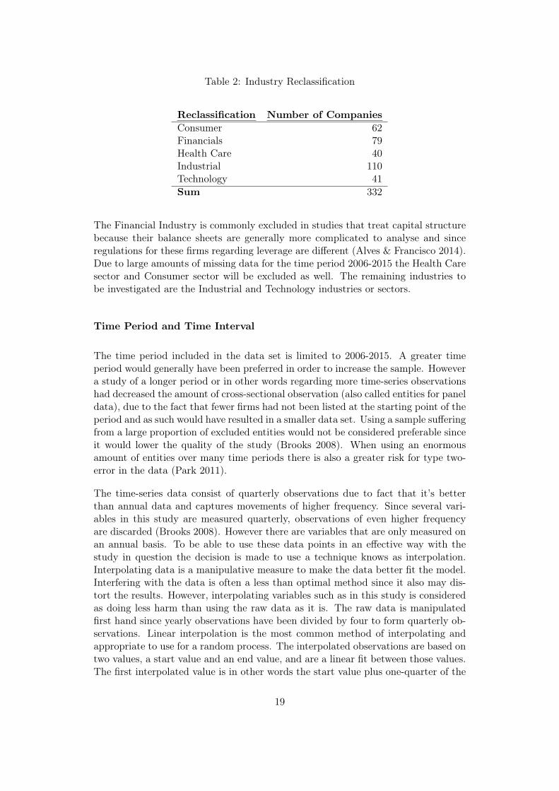
Table 2: Industry Reclassification

Reclassification Number of CompaniesConsumer 62Financials 79Health Care 40Industrial 110Technology 41Sum 332

The Financial Industry is commonly excluded in studies that treat capital structurebecause their balance sheets are generally more complicated to analyse and sinceregulations for these firms regarding leverage are different (Alves & Francisco 2014).Due to large amounts of missing data for the time period 2006-2015 the Health Caresector and Consumer sector will be excluded as well. The remaining industries tobe investigated are the Industrial and Technology industries or sectors.

Time Period and Time Interval

The time period included in the data set is limited to 2006-2015. A greater timeperiod would generally have been preferred in order to increase the sample. Howevera study of a longer period or in other words regarding more time-series observationshad decreased the amount of cross-sectional observation (also called entities for paneldata), due to the fact that fewer firms had not been listed at the starting point of theperiod and as such would have resulted in a smaller data set. Using a sample sufferingfrom a large proportion of excluded entities would not be considered preferable sinceit would lower the quality of the study (Brooks 2008). When using an enormousamount of entities over many time periods there is also a greater risk for type two-error in the data (Park 2011).

The time-series data consist of quarterly observations due to fact that it’s betterthan annual data and captures movements of higher frequency. Since several vari-ables in this study are measured quarterly, observations of even higher frequencyare discarded (Brooks 2008). However there are variables that are only measured onan annual basis. To be able to use these data points in an effective way with thestudy in question the decision is made to use a technique knows as interpolation.Interpolating data is a manipulative measure to make the data better fit the model.Interfering with the data is often a less than optimal method since it also may dis-tort the results. However, interpolating variables such as in this study is consideredas doing less harm than using the raw data as it is. The raw data is manipulatedfirst hand since yearly observations have been divided by four to form quarterly ob-servations. Linear interpolation is the most common method of interpolating andappropriate to use for a random process. The interpolated observations are based ontwo values, a start value and an end value, and are a linear fit between those values.The first interpolated value is in other words the start value plus one-quarter of the

19

difference between the start and end value, while the second interpolated value is thefirst interpolated value plus one-quarter of the difference between the start and endvalue. For every new entity the start and end value changes. Linear interpolation isdescribed by the function below:

z(t0 + i∆t) = zj′ +t0 + i∆t− tj′

tj′+1 − tj′(zj′+1 − zj′) (4)

Where z is the interpolated value, zj′ the start value and zj′+1 the end value. t0 tot0 + i∆t constitute the time period where every interpolated value is spaced by ∆t.The interpolation is done between the times tj′ and tj′+1 (Dacorogna et al. 2001).

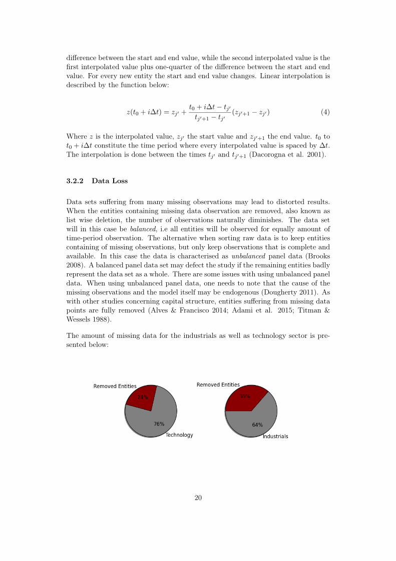
3.2.2 Data Loss

Data sets suffering from many missing observations may lead to distorted results.When the entities containing missing data observation are removed, also known aslist wise deletion, the number of observations naturally diminishes. The data setwill in this case be balanced, i.e all entities will be observed for equally amount oftime-period observation. The alternative when sorting raw data is to keep entitiescontaining of missing observations, but only keep observations that is complete andavailable. In this case the data is characterised as unbalanced panel data (Brooks2008). A balanced panel data set may defect the study if the remaining entities badlyrepresent the data set as a whole. There are some issues with using unbalanced paneldata. When using unbalanced panel data, one needs to note that the cause of themissing observations and the model itself may be endogenous (Dougherty 2011). Aswith other studies concerning capital structure, entities suffering from missing datapoints are fully removed (Alves & Francisco 2014; Adami et al. 2015; Titman &Wessels 1988).

The amount of missing data for the industrials as well as technology sector is pre-sented below:

20

3.3 Variables

3.3.1 Stock Returns

Return to investors are generated through capital gains, that is the change in stockprice from one time to another, plus the dividend paid over the time period inquestion. Total (simple) stock returns Rt includes dividends and is calculated asfollows:

Rt =(pt − pt−1) +D

pt−1(5)

Where p is the price at point t in time and t−1 one period behind (Finance Formulas[WEB]).

Since dividend yield significantly affects total stock return it is reasonable to includeit. If dividend yields are not taken into account, returns in many cases will beunderestimated, especially when returns are measured over longer holding periods.In case some companies in the data set employs regular dividend payments whileothers dont, excluding dividend yield may also have the effect of distorting thedata set and therefore results, favouring so called growth stocks over income stocksgenerally paying a high dividend yield (Brooks 2008). An alternative way to calculatetotal stock return is to use the formula (Finance Formulas [WEB]):

Rt = Capital Gains [%] + Dividend [%] (6)

In this study total stock return is used as a proxy for firm performance. Total stockreturns is based on figures from DataStream, function no. 6 is used for calculatingthis in the panel data.

3.3.2 Capital Structure

Capital structure, commonly known as leverage, can be measured as debt in relationto total assets (Titman & Wessels 1988; Rajan & Zingales 1995). In this study,book leverage figures will be used instead of market leverage figures, according toBarclay, Morellec & Smith Jr (2003) the book-leverage measure is better to use infinancial regressions since using market-based figures for the independent variablemight cause it to correlate spuriously with exogenous variables. Bowman on the otherhand shows that the correlation between book value and market value of debt arelarge and significant, indicating that using one over the other does not really matter(Bowman 1980). The Reuters DataStream codes are WC02999, WC03051, WC03251 andWC03255 for total assets, short-term debt, long-term debt and total debt respectively.Note that total debt doesn’t necessarily equal total liabilities, total debt representsall debt that is interest bearing plus capitalised obligations. Total liabilities onthe other hand also include other types of liabilities, such as pension obligations

21

etcetera (Thomas Reuters DataStream). Normally the debt ratio is measured astotal liabilities over total assets (Finance Formulas [WEB]).

Debt Ratio (Normal) =Total LiabilitiesTotal Assets

(7)

However in this study three debt ratios will be used in separate regressions, totaldebt ratio, long-term debt ratio as well as short-term debt ratio. Short-term debtrepresents the proportion of total debt that are expiring in one year meanwhilelong term debt is defined as interest bearing obligations of payments, excludinginterest bearing payments expiring up to one year (Thomas Reuters DataStream).In their study of small to medium sized companies, Cassar & Holmes suggest thatit is important to distinguish between long and short-term debt in the analysis.In particular for small and medium sized firms. Since this study includes small,medium and large companies it may be relevant to distinguish between the differentmeasurements (Cassar & Holmes 2003).

3.3.3 Control Variables

In a regression model of only one dependent and one independent variable it isimpossible to say if a relationship is true, even though correlation between themis high. To avoid this regression trap more explanatory variables, so called controlvariables are introduced and included in the regression model. A so called multipleregression model enables the researcher to distinguish between effects of the specificindependent variables. In this way the variables adjust for each other’s effects andeliminate unappreciated variables apparent effects (Dougherty 2011).

The explanatory variables in this study were found and chosen in accordance withearlier studies on the subject and are suggested to affect both a firm’s leverageratio and stock returns. The variables used are size, growth and market-to-bookratio. OMX30 total return index is used as an explanatory variable and proxy forgeneral market movements. The regressions will be done separately for the industrialindustry and the technology industry.

Size

Several studies suggest that capital structure to a certain extent correlates with firmsize. According to Titman and Wessels (1988) costs of debt are larger for smallerfirms, both in terms of bankruptcy and borrowing costs. This implies that smallercompanies should have a smaller proportion of debt than larger firms. In contrast totheir theoretical reasoning, Titman & Wessel (1988) and Rajan & Zingales (1995)find a negative relationship between size and leverage. However Cassar & Holmes(2003) find the relationship to be positive, but their evidence of this is weak.

Size is also an important control variable for a firms result since it effects capabilities,

22

benefits from diversification, economies of scale and credibility (Chadha & Sharma2015).

As in previous studies size is represented by the natural logarithm of sales since itreduces the amount of variation (Titman and Wessels 1988; Rajan & Zingales 1995;Cassar & Holmes 2003; Barclay, Morellec & Smith Jr 2003).

Growth

According to the pecking-order hypothesis, firms experiencing a relatively high growthshould be more open to financing their activities with equity than debt. Hence high-growth firms are often leveraged to a lesser extent (Brealey, Myers & Allen 2011).Growth is defined as the annual sales growth, i.e (Cassar & Holmes 2003):

Growthi =Net Salesi −Net Salesi−1

Net Salesi−1(8)

Titman and Wessel (1988) & Barclay, Morellec & Smith Jr (2003) are using prof-itability as a substitute for net sales growth. Their reasoning for not using both areto avoid multicolliniarity issues (see section 3.4.4 for further explanation).

Sales growth has a direct impact on a firm’s profitability, therefore the growth vari-able is a very significant control variable in the regression itself (Chadha & Sharma2015).

Market-to-Book

Market-to-book value is in this study used as a proxy for growth opportunities.Barclay, Morellec & Smith Jr (2003) use market-to-book as a proxy for growthoptions. Muradoglu & Sivaprasad (2012) use market-to-book-value to investigateif there is any relationship between leverage and stock returns (cumulative averageabnormal returns). They conclude that stock returns are higher for firms having lowdebt ratios and low market-to-book ratio. Rajan & Zingales (1995) also suggest thatthe relationship between market-to-book ratio and leverage is negative due to costsfor financial distress.

OMX30 Total Return Index

Since stock returns follow the general market to a certain extent a proxy for themarket can be included in the regression. The regression model will probably havea higher explanatory power with such a measurement included. Usually, a domesticstock market index is used as proxy for the entire market (Vishwanath 2007). Since

23

Swedish stocks are the ones focused upon in this paper it was natural to choose aSwedish stock index (OMX30) as the market proxy measurement.

This proxy will be the OMX30 total return index. OMX Stockholm 30 is the leadingindex on Nasdaq OMX Stockholm’s stock exchange and is based on market weightedprices of Nasdaq Stockholm’s 30 most traded stocks. The OMX30 total return indexis collected from DataStream (Thomas Reuters DataStream).

3.3.4 Industry Separation

Arditti (1967) proposes that risks are industry specific and therefore that the rela-tionship between stock return and leverage should be regarded separately for separateindustries. This study will follow Arditti’s position regarding this and be divided byindustries to take the eventual differences into account.

According to Hou & Robinson (2006) industry concentration, i.e. the degree of com-petetiveness in an industry, is an important determinating factor for stock returns.Firms in more competitive industries generally have higher returns than firms in lesscompetetive (low-concentrated) industries due to competitive pressure and a higherrisk of bankruptcy (Hou & Robinson 2006). Adami et al.’s (2015) findings suggestthat industry concentration not affect the relationship between stock returns andleverage. Zeitun & Tian (2007) find oppositedly that their included variable for in-dustry is statistically significant, which implies that industry has an effect on therelationship between stock returns and leverage.

3.4 Regression Model

3.4.1 Multiple Regression Model

This thesis will utilise a multiple regression model, an important statistical tool forempirical studies. A multiple regression model describes and evaluates the relation-ship between one dependent and a number of independent variables. In comparisonto a simple correlation analysis, the regression methodology assumes the dependentvariable to be random, in other words having a probability distribution. The inde-pendent variables however are assumed to be fixed. An analysis utilising multipleregression is more effective than doing a simple correlation analysis. Due to the factthat many independent variables can be included it is also a more flexible model.The general multiple regression model for panel data is (Brooks 2008):

24

yit = a0 + β1xit + β2xit + β3xit + ...+ βnxit + uit (9)

Where:y =Dependent Variablei =Observed Entityt =Time Perioda =Intercept Termβ =Coefficient to be estimated on the explanatory Variablesx =Independent Variableu =Disturbance Term

3.4.2 Choice of Model for Panel Data

There are several types of models available for panel data. The simplest one isthe pooled regression model. In this model entities are stacked together so that onecolumn contains all observations, both entities and time-series observations. In thisway the panel data will be defined as a single equation and an ordinary least squareregression (OLS) can be used to find a satisfactory equation. The drawback withthe pooled regression is that it assumes that the averages of the variables and therelation between the variables are fixed over both time and entities. This assumptionis often violated (Brooks 2008).

Another regression technique is to use the fixed effects model. A common form offixed effects model is known as the least square dummy variable model or LSDV forshort. In this model the disturbance terms are assumed to contain an individualspecific effect that could vary over both cross-section and time-series observations.The formula is specified as follows:

uit = µi + vit (10)

Where uit is the disturbance term, µi represents the individual specific effect and vitcaptures what is left from the disturbance term. Here µi varies across entities butnot time. The LSDV regression model is defined as:

yit = βxit + µ1D1i + µ2D2i + µ3D3i + ...+ µNDNi + vit (11)

In which D is a dummy variables substituting for the entities. The regression is fixedin terms of the cross-section observations. The fixed effects could also be adaptedto the time-series observations as a time-fixed effects model or as a two-way modelwhere both cross-sectional and time period observations are defined as fixed. To

25

investigate if a fixed-effect model or pooled OLS preferred, a redundant fixed effectstest could be performed with Eviews (Brooks 2008). Unfortunately, the fixed effectsmodel does not deal with heterogeneity. If the disturbance terms themselves arevery scattered in terms of variance and thus demonstrate heterogeneity, a third typeof model, the random effects model, may be a better fit than the fixed effects model.The random effects model provides a solution to the heterogeneity problem, it doeshowever require that it is possible to treat all of the unobserved variables as randomlydrawn and that they are distributed independently of all explanatory variables. Ifthose condition aren’t fulfilled the fixed effects model is to be preferred over therandom effects model (Dougherty 2011). To determine which model is most suitablefor estimating the equation a Hausman test could be performed with Eviews (Brooks2008).

In this analysis, the pooled and random effects models have been discarded due totheir bad fit. The redundant fixed effects test is significant meaning that the fixedeffect model is preferred to a pooled OLS. On the other hand the Hausman test isinsignificant and the random effects model is therefore not considered to be veryappropriate. An alternative to the fixed effect model could possibly have been thegeneralised least square model, also called the weighted least square model. In thismodel however it is of great importance that the dataset is not defected by manyoutliers. To justify using this model, the outliers must be investigated carefully andhandled correctly. Since it is difficult to define all outliers in panel data and sinceany data set (of this considerable size) contains at least a few outliers, the weightedleast square model is also discarded for this thesis (Brooks 2008).

3.4.3 Regression Specification

The research questions of this study is defined as follows:

• "How are stock returns affected by capital structure in Swedish listed firmsduring 2006-2015?"

• "Does the observed relationship between capital structure and stock returnvary between the industrial and the technology industry?"

The first research question is broken down to three sub-questions:

• "How does the total debt ratio affects stock returns?"

• "How does the long-term debt ratio affects stock returns?"

• "How does the short-term debt ratio affects stock returns?"

Three different regression models are going to be used. Control variables stay con-stant through all regressions while the debt variable varies between total debt ratio,

26

long-term debt ratio and short-term debt ratio. The regression models are presentedbelow. To take the industry effect into account the three regression models are ap-plied to both the industrial industry and the technology industry. The reason thatindustry is not included as a dummy is that it is problematic in combination withthe fixed effects mode l since it creates perfect multicollinearity between the dummyvariables.

Rit = a0 + β1TDTA it

+ β2Sit + β3Git + β4MTBit + β5OMXit + C + µit (12)

Rit = a0 + β1LTDTA it

+ β2Sit + β3Git + β4MTBit + β5OMXit + C + µit (13)

Rit = a0 + β1STDTA it

+ β2Sit + β3Git + β4MTBit + β5OMXit + C + µit (14)

R = Total returnTD/TA = Total debt / total assets

LTD/TA = Long-term debt / total assetsSTD/TA = Short-term debt / total assets

S = Size, natural logarithm of salesG = Growth, quarterly change in sales

MTB = Market-to-book valueOMX = OMX total return index

C = Crisis, dummy for the financial crisis

3.4.4 Significance Level

The significance level is a term describing the risk of there being a type 1 error inthe data when not rejecting the null hypothesis. For example a significance level of1% means that all values that are extreme will appear with a probability of 1%. Thecommon level of significance is 5% but when using a financial data set containinga large amount of observations, this can cause problems since standard errors tendto decrease when using large data sets. In case using large financial data sets thebetter way might be to set a 1% significance level (Brooks 2008). In this study both10%, 5% and 1% significance levels will be presented in the results.

3.4.5 Validity Tests

Robustness

In order to investigate if the regression models used are robust, i.e. not changingsignificantly when they are modified (White & Lu 2010) several checks and mod-

27

ifications have been made during the process. Control variables have been addedand removed one by one in order to investigate if the estimated coefficients change.Several variables have also been tested as different proxies. The variables for growthhas for example been tested both through the growth in net sales in line with Cassar& Holmes (2003) and by capital expenditures over total assets in line with Titman& Wessels (1988). The variable net sales growth were chosen due to the fact thatfigures for capital expenditures are more frequently missing. The potential controlvariable of non-debt tax-shields that Titman & Wessels (1988) use to explain capitalstructure is excluded since it does not fit well with the regression model. Tangi-bility, also used by Titman & Wessels (1988), is a proxy for asset structure and isalso excluded since it weakens several results in the regression model, especially ther-squared values. Since the remaining coefficients does not change considerably indirection of dependency or in magnitude during the modification tests the regressionmodel is estimated as robust, even though there a several pitfalls with this type ofrobustness check (White & Lu 2010).

The regression model is also tested for three different data sets: quarterly data,quarterly data with interpolated observations as well as annual data. The coefficientsare similar in regards to direction of influence and magnitude with a few exceptions,which also is good reason for justifying the regression model.

Normal distribution

An important assumption for ordinary least squares regressions is that the data setis normally distributed. If it is not or contains many so called outliers, values thatdoesn’t fit the distribution, the estimated coefficients of the regression model maybe seriously damaged. Excluding outliers may therefore improve the estimations ofthe regression model. There are different ways to dealing with outliers. One methodis to use a robust regression technique while another is to correct or delete outlyingvalues (Russeeuw 1987).

When using panel data it is hard to detect outliers. One method is to plot theresiduals in a histogram with Eviews (or your statistics tool of choice). If the residualshave the form of normally distributed varialbe but shows sign of skewness, the non-normality problem could be approached by excluding outliers causing skewness. Thismethod however is not ideal when using panel data since it is seldom enough fordetecting all outliers. Since there is little research on the subject regarding paneldata, this method will be used even in this thesis. To keep the data set balanced,whole entities will be excluded (Brooks 2008).

A third solution for dealing with non normal data may be to include a dummy-variable. For financial data dummy-variables are often used for adjusting for so calledextreme events. A financial crisis is a good example of such an event and justifiesthe use of a dummy variable (Brooks 2008). In this study, a dummy variable forcrisis will be included to adjust for outliers during the time period of the financialcrisis.

28

Near Multicollinearity

Near multicollinearity is when some of the explanatory variables in a multiple re-gression strongly correlate with each other. In case the multicollinearity is ignoredthe estimated coefficients may be somewhat erratic. The standard errors and ther-squared value will then normally be high and give the illusion that the test as awhole went well while the coefficients in actuality are not even significant. If thecorrelation between variables is small this issue could be ignored (Brooks 2008). Ac-cording to Kennedy (2011) variables that have a correlation below the absolute valueof 0.8 are valid. One simple method to detect multicollinearity is to calculate thecorrelations for all explanatory variables. Correlation matrixes will be presented insection 4.2.

Autocorrelation

An underlying assumption with regressions such as this is that the correlation be-tween the residuals are zero. If they aren’t the data suffers from autocorrelation,also called serial correlation. One way to detect autocorrelation is to use the Durbin-Watson test that tests for first order autocorrelation. The Durbin-Watson test prac-tically investigates the relationship between an errors current and previous value. Ifthe value of the Durbin-Watson test, is near 2, there is no clear evidence of auto-correlation in the disturbance terms. The value of zero is a sign of perfect positiveautocorrelation while the value of 4 on the other hand perfect negative autocorrela-tion (Brooks 2008).

Heteroscedasticity

Anonther assumption needing to be fulfilled justifying the estimations of a regressionmodel is that the variance of the standard errors is constant. This assumption isknown as homoscedasticity and the opposite, where the variance of standard errorschanges is called heteroscedasticity. If heteroscedasticity is ignored the coefficientswill be unbiased but inefficient. Normally a White test or an equivalent test is usedto investigate if the data suffers from heteroscedasticity (Brooks 2008). This solutionhowever is not available for panel data. Eviews instead offers the solution to adjustfor a robust estimation of heteroscedasticity with the White diagonal function. TheWhite diagonal function is used in this study to adjust for heteroskedasticity (EviewsUser’s guide).

Model fit

The r-squared value is a measure that indicates how well the regression model fits.A higher r-square generally equals a better fit. The r-squared value is at the sametime not really a key indicator of the model’s success. Even if the r-square is low,

29

the regression model could be adequate, as long as the estimated coefficients arestatistically significant (Dougherty 2011).

30

4 Empirical Findings

The following chapter will present descriptive statistics, multicollinearity matrixesand regression results. These findings will be the foundation upon which analysisand conclusions are built later on.

4.1 Descriptive Statistics

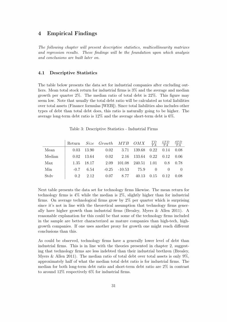
The table below presents the data set for industrial companies after excluding out-liers. Mean total stock return for industrial firms is 3% and the average and mediangrowth per quarter 2%. The median ratio of total debt is 22%. This figure mayseem low. Note that usually the total debt ratio will be calculated as total liabilitiesover total assets (Finance formulas [WEB]). Since total liabilities also includes othertypes of debt than total debt does, this ratio is naturally going to be higher. Theaverage long-term debt ratio is 12% and the average short-term debt is 6%.

Table 3: Descriptive Statistics - Industrial Firms

Return Size Growth MTB OMX TDTA

LTDTA

STDTA

Mean 0.03 13.90 0.02 3.71 139.68 0.22 0.14 0.08Median 0.02 13.64 0.02 2.16 133.64 0.22 0.12 0.06Max 1.35 18.17 2.09 101.08 240.51 1.01 0.8 0.78Min -0.7 6.54 -0.25 -10.53 75.9 0 0 0Stdv 0.2 2.12 0.07 8.77 40.13 0.15 0.12 0.08

Next table presents the data set for technology firms likewise. The mean return fortechnology firms is 4% while the median is 2%, slightly higher than for industrialfirms. On average technological firms grow by 2% per quarter which is surprisingsince it’s not in line with the theoretical assumption that technology firms gener-ally have higher growth than industrial firms (Brealey, Myers & Allen 2011). Areasonable explanation for this could be that some of the technology firms includedin the sample are better characterized as mature companies than high-tech, high-growth companies. If one uses another proxy for growth one might reach differentconclusions than this.

As could be observed, technology firms have a generally lower level of debt thanindustrial firms. This is in line with the theories presented in chapter 2, suggest-ing that technology firms are less indebted than their industrial brethren (Brealey,Myers & Allen 2011). The median ratio of total debt over total assets is only 9%,approximately half of what the median total debt ratio is for industrial firms. Themedian for both long-term debt ratio and short-term debt ratio are 2% in contrastto around 12% respectively 6% for industrial firms.

31

Table 4: Descriptive statistics - Technology Firms

Return Size Growth MTB OMX TDTA

LTDTA

STDTA

Mean 0.04 12.72 0.02 3.39 139.68 0.13 0.08 0.05Median 0.02 12.45 0.02 1.9 133.64 0.09 0.02 0.02Max 1.26 17.94 0.34 112.09 240.51 0.79 0.44 0.71Min -0.62 8.3 -0.44 -86.13 75.9 0 0 0Stdv 0.21 2.35 0.06 9.41 40.14 0.14 0.1 0.08

4.2 Near Multicollinearity

Like mentioned in section 3.4.4, a check againt near multicollinearity is performedto justify the use of the explanatory variables. In case two variables correlates withan absolute value of more than 0.8 one of the variables should be excluded (Kennedy2011).

The table below is a correlation matrix for industrial firms. As could be observed,no correlation is higher than 0.8 and most of the correlations are quite low. Thehighest correlation could be observed between the dummy variable crisis and theOMX30 total return index, -0.54. Since it is below the critical value both variablesare included in the regression model. There is a positive correlation of 0.27 betweenthe long-term debt ratio and size as well as 0.22 for total debt ratio and size.

Table 5: Correlation Matrix - Industrial Sector

Size Growth MTB OMX Crisis TDTA

LTDTA

STDTA

Size 1Growth -0.146 1MTB -0.1999 0.0393 1OMX 0.0456 0.0514 -0.0122 1Crisis -0.0074 -0.1614 -0.0475 -0.5446 1TD/TA 0.2176 -0.0855 -0.1139 0.0069 0.0543 1LTD/TA 0.2778 -0.0545 -0.1732 0.0185 0.0436 N.A 1STD/TA -0.0286 -0.0706 0.0554 -0.0143 0.0308 N.A N.A 1

Below is a similar table for technology firms. As for industrial firms, no correlationexeeds the criticual value of 0.8. The highest correlation is, as for industrial firms,observed between the dummy variable crisis and the OMX30 total return index, -0.55. The correlation between long-term debt and size is 0.4 and that between theshort-term debt ratio and market-to-book 0.23.

32

Table 6: Correlation Matrix - Technology Sector

Size Growth MTB OMX Crisis TDTA

LTDTA

STDTA

Size 1Growth -0.1511 1MTB -0.123 0.1464 1OMX30 0.0549 0.0034 -0.0344 1Crisis -0.0134 0.0337 0.0649 -0.5461 1TD/TA 0.1787 0.0298 0.0751 -0.0099 0.0058 1LTD/TA 0.4023 0.0372 -0.0661 0.0247 -0.0335 N.A 1STD/TA -0.1428 0.0187 0.2325 0.0004 0.0097 N.A N.A 1

4.3 Regression Results

In the following tables, the statistical regression results are presented for both in-dustrial firms and technology firms. The denotations of: *, ** or *** representsthe 10%, 5% and 1% significance levels. The upper figure for every variable is theestimated coefficient. If the figure is negative for a variable, the variable and stockreturns are negatively correlated. The figure below the estimated coefficient denotesthe p-value for each variable and constitutes the basis for the significance level.

4.3.1 Industrial Firms

Debt Ratios

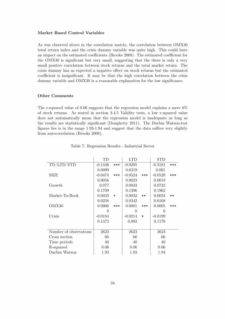
As can be observed in the table below, total debt and short-term debt correlatenegatively with stock return at a 1% significance level. The estimated coefficientfor total debt is -0.1446 and -0.3181 for short-term debt, indicating that short-termdebt ratio has a greater negative impact on stock returns than the total debt ratio.Long-term debt ratio also correlates negatively with stock return, but the result isstatistically insignificant.

Firm Specific Control Variables

Size has a negative impact on stock returns and is a reasonably good explanatoryvariable since the statistical significance is high in all of the three regressions. Growthestimates on the other hand are insignificant. The market-to-book estimates aresignificant at a lower level and suggest that there is a small yet positive correlationbetween market-to-book and stock returns.

33

Market Based Control Variables

As was observed above in the correlation matrix, the correlation between OMX30total return index and the crisis dummy variable was quite high. This could havean impact on the estimated coefficients (Brooks 2008). The estimated coefficient forthe OMX30 is significant but very small, suggesting that the there is only a verysmall positive correlation between stock returns and the total market return. Thecrisis dummy has as expected a negative effect on stock returns but the estimatedcoefficient is insignificant. It may be that the high correlation between the crisisdummy variable and OMX30 is a reasonable explanation for the low significance.

Other Comments

The r-squared value of 0.06 suggests that the regression model explains a mere 6%of stock returns. As stated in section 3.4.5 Validity tests, a low r-squared valuedoes not automatically mean that the regression model is inadequate as long asthe results are statistically significant (Dougherty 2011). The Durbin Watson-testfigures lies is in the range 1.93-1.94 and suggest that the data suffers very slightlyfrom autocorrelation (Brooks 2008).

Table 7: Regression Results - Industrial Sector

TD LTD STDTD/LTD/STD -0.1446 *** -0.0295 -0.3181 ***

0.0099 0.6319 0.001SIZE -0.0474 *** -0.0524 *** -0.0528 ***

0.0056 0.0023 0.0018Growth 0.077 0.0833 0.0722

0.1709 0.1396 0.1962Market-To-Book 0.0033 * 0.0032 ** 0.0034 **

0.0258 0.0342 0.0168OMX30 0.0006 *** 0.0001 *** 0.0005 ***

0 0 0Crisis -0.0184 -0.0214 * -0.0199

0.1472 0.092 0.1176

Number of observations 2623 2623 2623Cross section 66 66 66Time periods 40 40 40R-squared 0.06 0.06 0.06Durbin Watson 1.93 1.93 1.94

34

4.3.2 Technology Firms

Debt Ratios

As for industrial firms the estimated coefficients of all debt ratios are negative. Thep-values indicate that the coefficient for the short-term debt ratio and total debt ratiois significant. The coefficient for the short-term debt ratio of -0.5126 is significantat a 1% significance level while the coefficient for the total debt ratio -0.1968 is onlysignificant at a 6% level. As for industrial firms the estimated coefficient for thelong-term debt ratio is insignificant.

Firm Specific Control Variables

As for industrial firms the size variable has a negative impact on stock returns. Inthis case it is only significant regarding short-term debt ratio. In contrast to indus-trial firms the estimated coefficients for growth is highly significant and indicatesthat there is quite a high positive correlation between growth and stock returns fortechnology firms. The market-to-book estimates are insignificant for all three tests.

Market Based Control Variables

The estimated coefficients for the OMX30 Index is significant but very low as forindustrial firms and suggests that the there is only a very small positive correlationbetween stock returns and the total market return. The estimated coefficients ofcrisis are negative and insignificant. Since the correlation between OMX30 totalreturn index and the crisis dummy variable is quite high also for technology firms itis reasonable to believe that estimated coefficients for OMX30 and the crisis dummymay be distorted to a certain extent (Brooks 2008).

Other Comments

The r-squared values lie in the range 0.06-0.07 and suggest that the regression modelof stock return is explained by between 6-7%. As suggested above, a low r-squaredvalue does not automatically mean that the regression model is inadequate as longas the results are significant (Dougherty 2011). The Durbin Watson-test is in therange 2.12-2.14, suggesting that the data does not suffer from much autocorrelation(Brooks 2008).

35

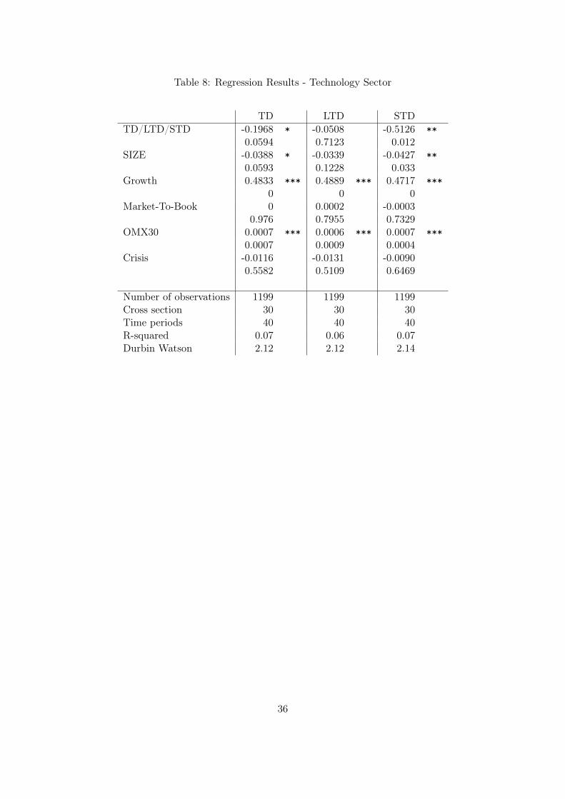
Table 8: Regression Results - Technology Sector

TD LTD STDTD/LTD/STD -0.1968 * -0.0508 -0.5126 **

0.0594 0.7123 0.012SIZE -0.0388 * -0.0339 -0.0427 **

0.0593 0.1228 0.033Growth 0.4833 *** 0.4889 *** 0.4717 ***

0 0 0Market-To-Book 0 0.0002 -0.0003

0.976 0.7955 0.7329OMX30 0.0007 *** 0.0006 *** 0.0007 ***

0.0007 0.0009 0.0004Crisis -0.0116 -0.0131 -0.0090

0.5582 0.5109 0.6469

Number of observations 1199 1199 1199Cross section 30 30 30Time periods 40 40 40R-squared 0.07 0.06 0.07Durbin Watson 2.12 2.12 2.14

36

5 Analysis & Discussion

Here the empirical results will be analysed in the context of theories and previousempirical findings that were presented in chapter 2. The purpose of the chapter is totie things up and give the reader a clear picture of how this study’s results relates toprevious results.

5.1 Stock Returns and Capital Structure

5.1.1 Total Debt Ratio

The regression results suggest that there is a negative relationship between totaldebt ratio and stock returns. H0: "That total debt-to-total assets ratio will notaffect stock returns significantly" is thus rejected. The results for industrial firmsare significant at a 1% level but only at a 6% significance level for technology firms.These results are in line with a majority of previous empirical studies on the subject(Arditti 1967; Hall & Weiss 1967; Adami et al. 2015; Penman, Richardson & Tuna2007; Acheampong, Agalega & Shibu 2013; Muradoglu & Sivaprasad 2012; George& Hwang 2009). Hamada (1969), Masulis (1983) and Bhandari (1988) however cameto the conclusion that leverage and stock returns correlate positively.

The results are inconsistent with the majority of accepted theories such as theModigliani & Miller theorem, the trade-off theory and the pecking order hypoth-esis. The Modigliani & Miller theorem suggests that firms that have a large amountof debt also should have high return due to the risk that comes with being leveraged.The trade-off theory suggests that this is the case at least up to a certain level ofdebt, the optimal debt level. A firm with a lower debt ratio should in accordancewiththis generate a lower return (Brealey, Myers & Allen 2011).

The results on the other hand are consistent with the market timing theory. Whichis if one recalls, that stock returns are supposed to correlate negatively with leveragesince managers tend to act irrationally and lower the debt ratio in times when thestock price is high (Brealey, Myers & Allen 2011). Several studies have demonstratedthat the market timing theory holds in reality. Masulis & Korwar (1986), Asquithand Mullins (1986) as well as Hovakimian, Hovakimian and Tehranian (2004) demon-strate that equity is issued more often in times when the stock price is high, sug-gesting that the stock price is high when the debt ratio is low and as such correlatesnegatively with leverage.

Adami et al. (2015) and Penman, Richardson & Tuna (2007) were expecting a pos-itive relationship between stock returns and leverage due to the higher risk leveragegenerates but observed the opposite. Adami et al. suggested that the oppositeresults best are explained by investors preferring to invest with firms who are finan-cially flexible and hence earn higher returns when doing so. Penman, Richardson &Tuna (2007) instead suggest that the unexpected relationship appears due to some

37

of the following reasons: 1) there are measurements errors in the leverage figures, 2)omittance risk factors negatively affect leverage or 3) the market generally mispricesleverage. George & Hwang (2009) suggest that the negative relationship is observeddue to the fact that investors may be compensated for other types of risks thanleverage risk.

Summary

The market timing theory and a few empirical studies satisfactorily explain thenegative relationship observed between stock returns and leverage. According to themarket timing theory leverage might negatively influence stock returns since firmmanagers time the market, lowering debt ratios via issuing more equity in timeswhen their respective stock prices are high.

Investors oddly enough seems to not be compensated for the additional risk thathigher leverage ratios supposedly entail. The reason may be that the market gen-erally misprices leverage or that investors preferences for high-leverage-stocks arelower and that these therefore yield lower returns due to the lower demand. A thirdoption for explaining the phenomena is that the higher observed stock returns forless leveraged firms could be compensation for investors for taking on other types ofrisks.

The relationship could further be explained by leverage figures suffering from mea-surement errors or that some control variables distort the results. Since differentempirical studies define leverage differently and use different methodologies for in-vestigating its potential effect on stock returns the results may differ somewhat.

5.1.2 Short-term and Long-term Debt Ratios

The estimated coefficients for both the long-term and short-term debt ratios arenegative for both industries. They are however only statistically significant for theshort-term debt ratios. These results contradict those of Gill, Biger & Mathur (2011)and Yazdanfar & Öhman (2015) that suggest short-term and long-term debt ratiosyield the same results. It has however been argued that long-term and short-termdebt should be investigated separately (Örtqvist 2006; Hall, Hutchinson & Michaelas2000). The results of this study suggest that long-term and short-term debt ratiosfare better by being separated since they yield different results.

The insignificant estimated coefficients for the long-term debt ratios suggest thatthere is no clear relationship between stock returns and long-term debt. H0: "Thelong-term debt ratio will not affect stock returns significantly" could thereby not berejected.

H0: "The short-term debt ratio will not affect stock returns significantly" is on theother hand rejected since the estimated coefficients for short-term debt ratios are

38

statistically significant at a 1% significance level.

5.2 Industry

The results suggests that the relationship between stock returns and leverage doesn’tdiffer between industrial and technology firms. The relationship is as stated in section4.3 negative both for total and short-term debt while insignificant regarding long-term debt. The estimated coefficient of the total debt ratio for technology firmsis not as significant as for industrial firms and the short-term debt ratio is morenegatively correlated to stock returns for technology firms. H0: "The impact ofleverage on stock return vary between industries" is therefore rejected. As pointedout in section 4.1, the theoretical assumption that technology firms should exhibithigher growth is not confirmed. This could possibly effect the regression results. Ifmany firms in the technology industry are characterised as mature firms rather thanhigh-tech, high-growth firms, there will practically be no industry effect in the data.It might also be possible that an industry effect had been observed if more industrieshad been included in the study.

These results contradicts Zeitun & Tian’s (2007). They come to the conclusion thattheir industry dummy variable is significant. The are however similar to Adami etal.’s conclusions (2015) which suggest that industry concentration doesn’t have anysignificant effect on the relationship between stock returns and leverage.

Control Variables

As could be observed in table 7 & 8 the significant explanatory variables are not thesame for technology firms as for industrial firms. It seems that growth is a decentexplanatory variable for technology firms, while not working well for industrial firms.On the ohter hand size seems to be a good explanatory variable for industrial firmsbut not as good for technology firms. These results suggest that the regression mighthave been better fitted if the growth variable was excluded for industrial firms andthe size variable was excluded for technology firms. These regression tests howeverweren’t performed since their results woulde been difficult to compare since theywould’ve been based on different sets of variables.

39

6 Conclusion

The concluding chapter attempts to reconnect with the research questions and presentconclusions drawn from the study. Ending with an explanation of the limitationsinvolved and presenting suggestions for further research on the subject.

6.1 General Thoughts

The purpose of this study was to investigate if there is a relationship between stockreturns and capital structure for Swedish firms listed on the Nasdaq OMX Stockholmstock exchange. The goal was to contribute with new research on a previously welldiscussed and researched subject on which former researchers results are inconclusive.The study also investigated if the relationship between stock returns and capitalstructure differs between the industrial and technology industries. Swedish paneldata was used in three different multiple regression models for each industry todistinguish between different types of debt ratios.

The results indicate that there is a negative relationship between leverage and stockreturns, suggesting that investors are not compensated for the leverage risk. Theseresults contradict accepted theories such as the Modigliani & Miller theorem, thetrade-off theory and the pecking- order hypothesis and question the common under-standing of capital structure. The results however are in line with the market timingtheory. Previous researchers such as Adami et al. (2015) and Penman, Richardson& Tuna (2007) have come to the same conclusion, suggesting that stock return cor-relates negatively with leverage. There are no significant observed differences in theresults between the industrial and technology industry.

Though there are interesting significancies regarding the question of whether on dealwith long or short term debt ratio. According to these results one should divide shortterm and long term debt separately. There might be - and there most certainly is- more to investigate and observe regarding short-term, total debt ratio differencesince their results differ so significantly. Short term debt ratio has a greater negativeeffect on stock return than total debt ratio (and by that reasoning also long termdebt ratios).

6.2 Limitations

Since results of previous empirical studies in some cases are contradictory it is dif-ficult to say what is actually correct. The conflicting results may come about dueto differences in methodologies and definitions regarding stock return and leverage.Additionally there are risks such as the relationship between stock returns and cap-ital structure suffers from a reversed association problem. The reversed associationproblem is present if capital structure affects stock returns at the same time as stockreturns affect capital structure.

40

Results may also be contradictory due to different samples. Since this study is limitedto using Swedish data and not is taking any country or cultural effect into account,it is difficult to say if the results are applicable to other countries. It is howeverreasonable to believe that they could be applicable to countries that are similar toSweden in term of business climate and culture. This argument is strengthened bythe fact that financing decisions to a large extent are based on international norms.

The results show that there is no direct industry effect on the relationship betweenstock returns and capital structure. Since the study is limited to investigating onlythe industrial and technology industries this conclusion is rather weak. More indus-tries would be preferable to investigate to be able to answer this question with agreater degree of certainty.

6.3 Future Research

Since capital structure is a factor concerning and influencing all firms, it will certainlyalways be an interesting topic to discuss and investigate. A way to dig deeper into thesubject is to do similar regressions with other variables. In this study debt to totalasset was used as a proxy for capital structure. Another ratio that also is commonlyused is the debt to equity ratio. It could be interesting to perform regressions withother explanatory variables. Since there is a large amount of pervious studies on thesubject there is also a large amount of control variables that have been tested andthat could be tested again on other data or in other combinations.

Few studies that have investigated the relationship between firm performance andcapital structure have used stock return as dependent variable. The majority haveinstead used book value measurements such as return on equity or return on assets.The majority of studies using stock return as dependent variable have also oftenused the expected stock return and CAPM as computation model of the variable.This study is conducted for actual stock returns and a suggestion for future studieswould be to further investigate this variable in relation to capital structure.

In addition, many of the performed studies on the relationship are now old andnot performed with panel data. A suggestion for further research is therefore toperform similar studies on more current data with more accurate methods. This maycontribute to a better understanding of todays relationship between stock return andcapital structure.

Furthermore, previous studies are limited regarding distinguishing between short-term and long-term debt ratios. In line with Örtqvist (2006) the results of this studysuggests that is important to distinguish between different types of debt ratios. Asuggestion for future studies would therefore be to look deeper into this problematicarea regarding capital structure.

As mentioned above this thesis is limited to investigating the industrial and tech-nology industries. To be able to better explain if industry has an effect on therelationship between stock returns and capital structure more industries could be

41

included in the investigation, perhaps in another part of the world or when moredata is readily avaliable?

42

7 References

7.1 Books

Brooks, C 2008, Introductory Econometrics for Finance, 2nd edition, pp. 7-8, 133-164, 171-174 & 487-510, Cambridge University Press, Cambridge

Baker, H K & Martin, G S 2011, Capital Structure and Corporate Financing De-cision: Theory, Evidence and Practise, pp. 75-90, John Wiley & Sons, Inc, NewJersey

Brealey, R A, Myers, S C & Allen, F 2011, Principles of Corporate Finance, 10thedition, pp. 440-465, McGraw-Hill/Irwin, New York.

Dacorogna, M M et al. 2001, An Introduction to High Frequency Finance, pp. 34-40,Academic Press

Dougherty, C 2011, Introduction to Econometrics, 4th edition, pp. 152-193 & 514-530, Oxford University Press, New York

Kennedy, P 2011, A Guide to Econometrics, 6th edition, pp. 196, Blackwell Pub-lishing

Koller, T & Goedhart, M 2010, "Valuation - Measuring and managing the value ofcompanies", 5th edition, pp. 17-57, Johan Wiley & Sons, Inc.

Russeeuw, PJ 1987, Robust Regressions and Outlier Detection, pp. 1-10, John Wiley& Sons Inc.

Saunders, M, Lewis, P & Thornhill, A 2009, Research Methods for Business Students,5th edition, pp. 106-161, Pearson Education Limited, Harlow

Vishwanath, S R 2007, Corporate Finance: Theory and Practice, pp. 86-90, SAGEPublications India

7.2 Online Journal Articles

Acheampong, P, Agalega E & Shibu, A K 2013, The Effect of Financial Leverageand Market Size on Stock Return on the Ghana Stock Exchange: Evidence fromSelected Stocks in the Manufacturing Sector, Pp. 125-134, International JournalOf Financial Research, Available From: //Www.sciedupress.com/journal/index.php/ijfr/article/viewFile/3973/2344 [Accessed: 28 August 2016]

Alves, P & Francisco, P 2014, The Impact of Institutional Environment on the Capi-tal Structure of Firms During Recent Financial Crises, Available from: https://www.researchgate.net/profile/Paulo_Alves29/publication/282092060_The_Quarterly_Review_of_Economics_and_Finance/links/5602b32908ae3b544e3517e3.pdf [Ac-

43

cessed: 15 July 2016]

Asquith, P & Mullins D W 1986, Equity Issues and Offering Dilution, pp. 61-89, Journal of Finance Economics 15, Available from: http://schwert.simon.rochester.edu/f423/jfe86_am.pdf [Accessed: 10 August 2016]

Barclay, M J, Morellec, E & Smith Jr, C W 2003, On the Debt Capacity of GrowthOptions, Journal of Business, Available from: https://www.researchgate.net/profile/Clifford_Smith3/publication/5021515_On_the_debt_Capacityof_growth_Options/links/54fd916f0cf270426d12994e.pdf [Accessed:11 July 2016]

Bowman, R G 1980, The Importance of a Market-value Measurement of Debt inAssessing Leverage, pp. 242-254, Journal of Accounting Research, Available from:https://www.researchgate.net/profile/Robert_Bowman4/publication/253644491_The_Importance_of_a_Market_Value_Measurement_of_Debt_in_Assessing_Leverage/links/5548d0630cf2f72b5d43535a.pdf [Accessed: 4 August 2016]

George, T J & Hwang, C Y 2009, A Resolution of the Distress Risk and LeveragePuzzles in the Cross Section of Stock Returns, The Journal of Financial Economics,Available from: http://citeseerx.ist.psu.edu/viewdoc/download?doi=10.1.1.452.8994&rep=rep1&type=pdf [Accessed: 12 August 2016]

Graham, J R & Harvey, C R 2001, The Theory and Practice of Corporate Finance:Evidence from the Field, pp. 187-243, Journal of Financial Economics 60, Availablefrom: http://publicsde.regie-energie.qc.ca/projets/72/DocPrj/R-3807-2012-C-ACIG-0059-DDR-REPDDR-2012_12_20.pdf [Accessed: 10 August 2016]

Hamada, R S 1969, Portfolio Analysis, Market Equilibrium and Corporate Finance,pp. 13-31, The Journal of Finance Vol. 24, Available from: http://ecsocman.hse.ru/data/856/126/1231/hamada_-_cs_1969.pdf [Accessed: 10 August 2016]

Hou, K & Robinson, D T 2006, Industry Concentration and Average Stock Re-turn, The Journal of Finance 4, Available from: http://citeseerx.ist.psu.edu/viewdoc/download?doi=10.1.1.163.2818&rep=rep1&type=pdf [Accessed:5 July 2016]

Masulis, R W 1983, The Impact of Capital Structure Change on Firms Value: SomeEstimates, pp. 107-126, The American Finance Association, Available from: http://citeseerx.ist.psu.edu/viewdoc/download?doi=10.1.1.477.4201&rep=rep1&type=pdf [Accessed: 28 June 2016]

Masulis, R W & Korwar, A N 1986, Seasoned Equity Offerings: an Empirical Inves-tigation, pp. 91-118, Journal of Finance Economics 15, Available from: http://219.219.114.96/cufe/upload_files/file/20140522/3_20140522_32%20Seasoned%20equity%20offeringsAn%20empirical%20investigationOriginal%20Research%20Article.pdf [Accessed: 10 August 2016]

Miller, M H1988, The Modigliani-Miller Propositions after Thirty Years, pp. 99-120,Journal of Economic Perspectives Vol. 2, Available from: http://vip.opload.ir/vipdl/94/4/zohreh/The-Modigliani-Miller-Propositions-After-Thirty-Years.

44

pdf [Accessed: 10 June 2016]

Muradoglu & S. Sivaprasad, Y G 2012, Using Firm-leverage as an Investment Strat-egy, pp. 260-279, Journal of Forecasting 31, Available from: https://www.researchgate.net/profile/Gulnur_Muradoglu/publication/228255746_Using_Firm_Level_Leverage_as_an_Investment_Strategy/links/0fcfd5086c228e5f96000000.pdf [Accessed:12July 2016]

Myers, S C 1984, The Capital Structure Puzzle, pp. 575-592, Journal of Finance39. Available from: http://lib.cufe.edu.cn/upload_files/file/20140522/3_20140522_35%20Myers,%20Stewart%20C.,%201984,%20The%20capital%20structure%20puzzle.pdf [Accessed: 15 June 2016]

Park, M H 2011, Practical Guides to Panel Data Modelling: A Step by Step AnalysisUsing Stata, Available from: https://webcache.googleusercontent.com/search?q=cache:sP25oHCgfqEJ:https://www.researchgate.net/file.PostFileLoader.html%3Fid%3D5688ff2960614b26808b4575%26assetKey%3DAS%253A313764916727808%25401451818793701+&cd=1&hl=en&ct=clnk&gl=se [Accessed: 13 July 2016]

Penman, S H, Richardson S A & Tuna, I 2007, The Book-to-price Effect in StockReturns: Accounting for Leverage, Journal of Accounting Research vol. 45, Avail-able from: http://citeseerx.ist.psu.edu/viewdoc/download?doi=10.1.1.421.4711&rep=rep1&type=pdf [Accessed: 28 June 2016]

Rajan, R G & Zingales, L 1995, What do We Know about Capital Structure?Some Evidence from International Data., pp. 1421-1460, The Journal of Finance,Available from: http://faculty.chicagobooth.edu/raghuram.rajan/research/papers/paper4.pdf [Accessed:28 July 2016]

Shyam-Sunder, L & Myers, S C 1999, Testing Static Trade-off against Pecking Or-der Models of Capital Structure, pp. 219-244, Journal of Finance Economics 51,Available from: http://pages.stern.nyu.edu/~eofek/PhD/papers/SM_Testing_JFE.pdf [Accessed: 17 June 2016]

Sparrow, E 2013, "What drives business values?", Available from: http://www.grantthornton.co.nz/Assets/documents/sectors/what-drives-business-value.pdf [Accessed: 11 August 2015]

Titman, S & Wessels, R 1988, The Determinants of Capital Structure Choice, pp. 1-19, The Journal of Finance, Available from: http://links.jstor.org/sici?sici=0022-1082%28198803%2943%3A1%3C1%3ATDOCSC%3E2.0.CO%3B2-A [Accessed:11 July2016]

White, H & Lu, X 2010, Robustness Checks and Robustness Tests in Applied Eco-nomics, Journal of Econometrics, Available from: http://www.economics.uci.edu/files/docs/micro/s11/white.pdf [Accessed: 2 August 2016]

Zeitun, R & Tian, G G 2007, Capital Structure and Corporate Performance: Ev-idence from Jordan, Australian Accounting, Business and Finance Journal, Available

45

from: http://ro.uow.edu.au/cgi/viewcontent.cgi?article=1018&context=aabfj[Accessed: 30 July 2016]

7.3 Printed Journal Articles

Adami, R, Gough, O, Muradoglu, Y G & Sivaprasad, S. 2015, How does a Firm’sCapital Structure affect Stock Performance? Available from: Lund University Li-braries

Arditti, F D 1967, Risk and the Required Return on Equity, Available from: LundUniversity Libraries

Artikis P G & Nifora, G 2011, The Industry Effect on the Relationship betweenLeverage and Returns, pp. 125-145, Eurasian Business Review. Available from:Lund University Libraries

Bhandari, L C 1988, Debt/Equity Ratio and Expected Common Stock Returns: Em-pirical evidence, The Journal of Finance vol. XLIII, Available from: Lund UniversityLibraries

Cassar, G & Holmes, S 2003, Capital Structure and Financing of SMEs: AustralianEvidence, pp. 123-147, Accounting and Finance 43, Available from: Lund UniversityLibraries

Chadha, S & Sharma, A K 2015, Capital structure and Firm Performance: EmpiricalEvidence from India, SAGE Publications, Available from: Lund University Libraries

Gill, A, Biger, N & Mathur, N 2011, The Effects of Capital Structure on Profitability:Evidence from the United States, International Journal of Management vol. 28,Available from: Lund University Libraries

Gupta, M C 1969, The Effect of Size, Growth, and Industry on the Financial Struc-ture of Manufacturing Companies, pp. 517-529, The Journal of Finance, Availablefrom: Lund University Libraries

Hall, G, Hutchinson, P & Michaelas, N 2000, Industry Effects on the Determinantsof Unquoted SME’s Capital Structure, pp. 297-312, International Journal of theEconomics of Business 3, Available from: Lund University Libraries

Hall, M & Weiss, L 1967, Firm Size and Profitability, pp. 319-331, The Review ofEconomics and Statistics, Available at: Lund University Libraries

Hovakimian, A, Hovakimian, G & Tehranian, H 2004, Determinants of Target Cap-ital Structure: the Case of Dual Debt and Equity Issues, pp. 517-540, Journal ofFinance Economics Vol. 71, Available from: University Libraries

Hovakimian, A, Opler, T & Titman, S 2001, The Debt-equity Choice, The Journalof Financial and Quantitative Analysis Vol.36, Available from: Lund University

46

Libraries

Jensen, M C & Meckling, W H 1976, Theory of the Firm: Managerial Behaviour,Agency Costs and Ownership Structure, pp. 305-360, Journal of Financial Eco-nomics 3, Available from: Lund University Libraries

Modigliani, F & Miller, M H 1958, The Cost of Capital, Corporation Finance andthe Theory of Investment, pp. 261-297, The American Economic Review vol. 48Available from: Lund University Libraries

Yazdanfar, D & Â. . . hman, P 2015, Debt Financing and Firm Performance: anEmpirical Study Based on Swedish Data", Pp. 102-118, The Journal Of Risk FinanceVol.16, Available From: Lund University Libraries

Örtqvist, D 2006, Determinants of Capital Structure in New Ventures: Evidence fromSwedish Longitudinal Data, pp. 277-296, Journal of Developmental Entrepreneur-ship 4. Available from: Lund University Libraries

7.4 Websites

Eviews User’s Guide, Estimation Background, Available from: http://www.eviews.com/help/helpintro.html#page/content/panel-Estimation_Background.html [Ac-cessed: 30 June 2016]

Finance Formulas, Total Stock Return, Available from: http://www.financeformulas.net/Total-Stock-Return.html [Accessed: 14 July 2016]

Financial Times, Financial Times lexicon, Available from: http://lexicon.ft.com/Term?term=corporate-capital-structure [Accessed: 16 July 2016]

Nasdaq OMX Nordic, Companies Listed on Nasdaq Stockholm, Available from:http://www.nasdaqomxnordic.com/aktier/listed-companies/stockholm [Accessed:2 July 2016]

Research Methodology, Research Approach, Available from: http://research-methodology.net/research-methodology/research-approach/ [Accessed: 13 July 2016]

7.5 Databases

Thomas Reuters DataStream, Available from: Lund University [Accessed: 10 June2016]

47