THE EFFECTS OF FAIRNESS PERCEPTION OF …vuir.vu.edu.au/15214/1/Aryani.pdf · THE EFFECT OF...

THE EFFECT OF FAIRNESS PERCEPTION OF

PERFORMANCE MEASUREMENT IN THE BALANCED SCORECARD ENVIRONMENT

By

Y Anni Aryani

B.A. (Accounting), Sebelas Maret University, Indonesia Master of Professional Accounting, Queensland University, Australia

This thesis is presented in fulfilment of the requirements of the degree of

Doctor of Philosophy

School of Accounting Faculty of Business and Law

Victoria University Melbourne, Australia

2009

Acknowledgments

Many people and institutions have made valuable contributions to this research.

Without their support and encouragement, it would have been very hard for me

to complete this research, which at times seemed never ending. Therefore, I

would like to take this opportunity to gratefully acknowledge those whose

contributions were significant to the successful completion of this thesis.

I would firstly like to express my heartfelt thanks to my supervisors, Dr Albie

Brooks, Professor Bob Clift and Dr Judy Oliver.

Dr Albie Brooks was my principal supervisor before moving to Melbourne

University. His valuable support, advice and encouragement during the first two

years of this research, successfully guided me through the ups and downs of the

PhD journey. Without his continual good advice and critical thoughtful scrutiny

of the whole written document, this thesis would have taken much longer to

finish.

Professor Bob Clift is my current principal supervisor. Professor Clift provided

me with good advice and support which made the completion of this thesis

possible. He patiently read through each of the chapters and provided

intellectually stimulating comments. His broad experience and skills in

supervising of PhD research has given me confidence regarding my thesis.

Dr Judy Oliver was my co-supervisor. She provided me with good support,

advice and encouragement during the beginning state of my PhD. She continued

to provide me with valuable feedback even after her move to Swinburne

University.

Secondly, I would like to thank Dr Rodney Turner who was a lecturer at the

School of Information Systems at Victoria University. He provided me with

valuable feedback during the statistics section, especially in Structural Equation

Modelling (SEM) with AMOS. He utilised his many years of knowledge and

experience in this area to help me pass through the difficulties I encountered

ii

using SEM. Without his help and support it would not have been possible for me

to finish this at this time.

Thirdly, I would also like to thank Dr Segu Zuhair who is a senior lecturer at the

School of Economics and Finance at Victoria University. He provided me with

valuable comments on my framework development during the beginning stage of

this thesis.

Fourthly, I would like to thank the Technological and Professional Skills

Development Project (TPSDP) and the Indonesian Government, via Ditjen

Pendidikan Tinggi (DIKTI), for providing me with a scholarship to undertake the

PhD. I am grateful to all the staff at the Accounting Department in Sebelas Maret

University, especially Drs Santoso Trihananto, Msi Ak, who provided me with

administration support regarding the scholarship. I also would like to thank the

Australian Federation of University Women (AFUW) – Victoria for providing

me with additional financial support during the research process.

Victoria University also deserves my sincere thanks for providing me with very

good facilities, especially for a disabled person like myself. This enabled me to

embark on interesting and practically important research. For that reason, I

would like to thank all of the disability unit staff at Victoria University. I also

would like to thank Ms. Tina Jeggo who is the student advice officer – research,

in the Business and Law Faculty. She is a very kind person who provided me

with a lot of support, advice, encouragement and help during my study period in

this university. I would also like to thank Ms. Rekha Vas from the School of

Accounting, who provided me with administration support in conducting this

research.

On many occasions I have had various versions of this thesis, and other work,

closely edited by Dr Riccardo Natoli. I have always felt humbled by the care in

which he reviewed my work. Many thanks for your friendship, kindness, sharing

of knowledge and everything else.

iii

Special thanks to all of my friends, who I can not mention one by one, for their

encouragement, support, and helpful comments. Without you all, I am sure it

would have been hard for me to live in Melbourne, which is very far from my

home town of Solo, Indonesia, to study for my PhD degree.

I owe a great debt to my family. My father and mother, Bapak Sriyoso and Ibu

Widarti, have given me the confidence to pursue my dreams. Their own strength

and fortitude has been an inspiration. I am also grateful for the continual support

and encouragement of my brothers Yos and Harin, my sister Enni, my sisters in

law Susi and Tiwi, my brother in law Edy, my nieces Vira, Yoesti, Hanin,

Hendras, Lintang and my nephews Agil and Fikri during this period of study.

How lucky I am to belong to this wonderful family. I love you all.

Finally, the greatest amount of thanks goes to my God, Allah SWT. Thanks my

God, for leading me on the full assurance in belief, so that a matter of hope has

become a matter of certainty.

I sincerely thank you all.

iv

Declaration

“I, Y Anni Aryani, declare that the PhD thesis entitled “The Effect of Fairness

Perception of Performance Measurement in the Balanced Scorecard

Environment” is no more than 100,000 words in length including quotations and

exclusive of tables, figures, appendices, bibliography, references and footnotes.

This thesis contains no material that has been submitted previously, in whole or

in part, for the award of any other academic degree or diploma. Except where

otherwise indicated, this thesis is my own work”.

Y Anni Aryani ………………………………Date………………….March 2009

v

Publications associated with this thesis

Conference Paper

Aryani, A., Brooks, A. and Oliver, J. 2008 “A Framework to Investigate the

Effects of Fairness Perception of Performance Measurement in the Balanced

Scorecard Environment”, Global Accounting & Organisational Change

Conference, Hilton on the Park, Melbourne, Australia.

vi

Table of Contents Page

Acknowledgments ................................................................................... .... ii

Declaration ................................................................................................ .... v

Publication Associated with Thesis ........................................................ .... vi

Table of Contents ..................................................................................... .... vii

List of Tables ............................................................................................ .... xv

List of Figures ........................................................................................... .... xviii

Abstract ..................................................................................................... .... xx

List of Abbreviations ............................................................................... .... xxiii

Chapter 1: Introduction .......................................................................... .... 1

1.1 Background to the Research .............................................. .... 1

1.2 Research Problem .............................................................. .... 2

1.3 Objectives of the Study ...................................................... .... 2

1.4 Significance of the Study ................................................... .... 3

1.5 Contributions of the Research ............................................ .... 4

1.6 Scope of the Research ........................................................ .... 4

1.7 Definition of Key Terms .................................................... .... 4

1.8 The Organisation of the Thesis .......................................... .... 6

Chapter 2: Literature Review: The Balanced Scorecard and Its Common-

Measure Bias Problem ......................................................... .... 10

2.1 Introduction ........................................................................ .... 10

2.2 Review of Performance Measurement Systems ................. .... 10

2.2.1 Limitations of Traditional Performance Measurement

System .................................................................... .... 11

2.2.2 Financial and Non-Financial Measures .................. .... 13

2.3 The Balanced Scorecard and Its Adoption ......................... .... 19

2.3.1 What Is the Balanced Scorecard? ........................... .... 20

2.3.1.1 Financial Perspective ................................. .... 22

2.3.1.2 Customer Perspective ................................. .... 22

2.3.1.3 Internal Business Process Perspective ....... .... 22

vii

3.1.4 Learning and Growth Perspective ................... 24

2.3.2 The Balanced Scorecard Adoption .............................. 25

2.4 Common-Measure Bias in Balanced Scorecard ...................... 27

2.4.1 Common-Measure Bias Phenomenon ......................... 27

2.4.2 Common-Measure Bias and the Balanced Scorecard . 29

2.4.3 Some Approaches to Overcome the Common-Measure

Bias Phenomenon ........................................................ 30

2.4.4 The Weighting Issue of Performance Measures ......... 37

2.5 Summary ................................................................................. 37

Chapter 3: Literature Review: Fairness Perception, Trust and Managerial

Performance .............................................................................. 39

3.1 Introduction ............................................................................. 39

3.2 The Drivers of Perceptions of Fairness ................................... 39

3.2.1 Organisational Fairness ............................................... 41

3.2.1.1 Reactive Content Theory ................................. 42

3.2.1.2 Proactive Content Theory ............................... 44

3.2.1.3 Reactive Process Theory ................................. 45

3.2.1.4 Proactive Process Theory ................................ 47

3.2.2 Distributive and Procedural Fairness .......................... 48

3.2.3 Distributive Fairness ................................................... 49

3.2.4 Procedural Fairness ..................................................... 51

3.2.5 Participation ................................................................. 54

3.3 Trust and Performance Evaluation .......................................... 57

3.4 Managerial Performance ......................................................... 64

3.5 Summary ................................................................................. 67

Chapter 4: Research Framework ................................................................ 68

4.1 Introduction ............................................................................. 68

4.2 Research Question ................................................................... 68

4.3 Research Framework ............................................................... 70

4.4 Hypothesis Development ........................................................ 72

viii

4.1 Participation, Common-Measure Bias, Fairness

Perception and Trust ................................................... 72

4.4.2 Managerial Performance ............................................. 74

4.5 Operationalisation of the Key Constructs ............................... 76

4.6 Participation ............................................................................ 77

4.6.1 The Instrument ............................................................ 77

4.7 Financial and Non-Financial Performance Measures ............. 78

4.7.1 The Use of Performance Measures ............................. 78

4.7.2 General Perception Relating to Performance Measures 79

4.7.3 Financial and Non-Financial Measures ....................... 79

4.8 Fairness Perception ................................................................. 80

4.8.1 Procedural Fairness ..................................................... 80

4.8.1.1 The Instrument ................................................ 80

4.8.2 Distributive Fairness ................................................... 81

4.8.2.1 The Instrument ................................................ 81

4.8.3 Fairness of Financial vs. Non-Financial Measures ..... 81

4.8.3.1 The Instrument ................................................ 82

4.9 Interpersonal Trust .................................................................. 82

4.9.1 The Instrument ............................................................ 82

4.10 Managerial Performance ......................................................... 82

4.10.1 Division (Unit) Manager Perception of Their

Performance ................................................................ 83

4.10.2 Managerial Performance Based on Division Manager’s

View of Senior Manager’s Perception ........................ 84

4.11 Summary ................................................................................. 85

Chapter 5: Research Method ....................................................................... 87

5.1 Introduction ............................................................................. 87

5.2 The Research Method ............................................................. 87

5.2.1 Why a Survey Method? ............................................... 87

5.2.2 Why a Mail Questionnaire? ........................................ 89

5.3 Data Quality ............................................................................ 90

ix

3.1 Measurement Error ..................................................... 90

5.4 The Population and Unit of Analysis of the Survey ............... 91

5.5 The Questionnaire ................................................................... 92

5.5.1 Development of the Questionnaire ............................. 92

5.5.2 Pilot Testing ................................................................ 94

5.6 The Sample ............................................................................. 96

5.6.1 Sample Selection ......................................................... 96

5.6.1.1 The Sampling Frame ....................................... 96

5.6.1.2 The Sampling Method ..................................... 96

5.6.2 Sample Size ................................................................. 97

5.6.2.1 Statistical Power and the Number of Firms

Selected ........................................................... 97

5.6.3 Sample Details ............................................................ 98

5.7 Administration of the Survey .................................................. 98

5.7.1 The Initial Mail-Out .................................................... 99

5.7.2 Follow-up Procedures ................................................. 101

5.7.3 The Final Sample ........................................................ 103

5.7.4 Sampling Error ............................................................ 104

5.7.4.1 Non-Response ................................................. 105

5.8 Data Editing and Coding ......................................................... 106

5.9 Data Screening ........................................................................ 106

5.9.1 Initial Data Screening .................................................. 106

5.9.2 Missing Data ............................................................... 106

5.9.3 Multi-variate Outliers .................................................. 108

5.9.4 Multi-variate Normality .............................................. 109

5.9.5 Multi-collinearity ........................................................ 111

5.10 Generalisability of the Findings .............................................. 111

5.11 Data Analysis .......................................................................... 112

5.11.1 Structural Equation Modelling (SEM) ........................ 113

5.11.2 Bootstrapping Procedures and Bollen-Stine Bootstrap

Method ........................................................................ 114

5.11.3 Sample Size Requirements .......................................... 115

x

12 Ethics in this Research ............................................................ 115

5.13 Summary ................................................................................. 115

Chapter 6: Descriptive Analysis .................................................................. 117

6.1 Introduction ............................................................................. 117

6.2 Respondents ............................................................................ 117

6.2.1 Companies ................................................................... 118

6.2.2 Divisions (Business Units) .......................................... 118

6.2.3 Division (Business Unit) Output Transfer Internally .. 119

6.2.4 Division’s Manager ..................................................... 120

6.2.4.1 Gender ............................................................. 120

6.2.4.2 Age .................................................................. 120

6.2.4.3 Period in Current Position ............................... 121

6.2.4.4 Duration Employed in the Company ............... 121

6.2.4.5 Number of Employees .................................... 122

6.3 General Perceptions Relating to Performance Measures ........ 122

6.4 Financial and Non-Financial Measures ................................... 123

6.4.1 Financial Measures Perspective .................................. 124

6.4.2 Customer Measures Perspective ................................. 126

6.4.3 Internal Business Process Perspective ........................ 127

6.4.4 Learning and Growth Perspective ............................... 128

6.5 Reliability Analysis ................................................................. 129

6.6 Summary ................................................................................. 130

Chapter 7: Preliminary Analysis ................................................................. 132

7.1 Introduction ............................................................................. 132

7.2 Constructs of the Research Model .......................................... 132

7.3 Constructs Reliability .............................................................. 134

7.4 Measure of Model Fit .............................................................. 134

7.5 Discriminant Validity .............................................................. 136

7.5.1 Single-Factor Congeneric Model ................................ 136

xi

5.1.1 Single-Factor Congeneric Model of

Participation (PRTCPT) .................................. 137

7.5.1.2 Single-Factor Congeneric Model of

Procedural Fairness (PFAIR) .......................... 141

7.5.1.3 Single-Factor Congeneric Model of Trust

(TRST) ............................................................ 143

7.5.1.4 Single-Factor Congeneric Model of Use of

Performance Measure (CMB) ......................... 145

7.5.1.5 Single-Factor Congeneric Model of Managerial

Performance Based on Division Manager’s

Self-Assessment (MPD) ................................... 146

7.5.2 Confirmatory Factor Analysis (CFA) .......................... 147

7.5.2.1 Confirmatory Factor Analysis of Procedural

Fairness Model ............................................... 148

7.5.2.1.1 Procedural Fairness Model with

MPD .............................................. 149

7.5.2.1.2 Procedural Fairness Model with

MPS ............................................... 152

7.5.2.2 Confirmatory Factor Analysis of Distributive

Model .............................................................. 155

7.5.2.2.1 Distributive Fairness Model with

MPD .............................................. 156

7.5.2.2.2 Distributive Fairness Model with

MPS ............................................... 158

7.6 Summary ................................................................................. 161

Chapter 8: Fairness Perception Model ....................................................... 162

8.1 Introduction ............................................................................. 162

8.2 Model Estimation .................................................................... 162

8.2.1 Standardised and Unstandardised Structural (Path)

Coefficients ................................................................. 162

8.2.2 Squared Multiple Correlations (SMC) ........................ 163

xii

3 The Proposed Research Model ................................................ 164

8.4 A Full Structural Model .......................................................... 169

8.5 Procedural Fairness Model ...................................................... 170

8.5.1 Procedural Fairness (PFAIR) – MPD Model .............. 171

8.5.1.1 Mediator Variable ........................................... 179

8.5.2 Procedural Fairness (PFAIR) – MPS Model ............... 184

8.6 Distributive Fairness Model .................................................... 193

8.6.1 Distributive Fairness (DFAIR) – MPD Model ........... 193

8.6.2 Distributive Fairness (DFAIR) – MPS Model ............ 201

8.7 Fairness of Financial vs. Non-Financial Measures ................. 209

8.8 Summary ................................................................................. 211

Chapter 9: Discussions, Conclusions and Suggestions .............................. 214

9.1 Introduction ............................................................................. 214

9.2 Key Findings of Demographic Characteristics ....................... 214

9.2.1 The Companies and the Divisions .............................. 214

9.2.2 The Division Managers ............................................... 214

9.2.3 Divisional Managers’ General Perceptions Regarding

Performance Measures ................................................ 215

9.2.4 The Performance Measures ......................................... 215

9.3 The Fairness Perception Model ............................................... 216

9.3.1 Results of Hypotheses Testing with the Procedural

Fairness Model ............................................................ 218

9.3.2 Results of Hypotheses Testing with the Distributive

Fairness Model ............................................................ 224

9.3.3 Financial vs. Non-Financial Fairness .......................... 229

9.3.4 Summary of the Hypotheses Testing Findings ........... 230

9.4 Research Implications ............................................................. 231

9.4.1 Theoretical Implications ............................................. 231

9.4.2 Methodological Implications ...................................... 233

9.4.3 Practical Implications .................................................. 233

9.5 Limitations of the Study .......................................................... 234

xiii

xiv

Page

9.6 Suggestions for Further Research ........................................... 235

9.7 Summary ................................................................................. 236

References ...................................................................................................... 237

Appendices ..................................................................................................... 260

APPENDIX I ................................................................................................... 260

Part A: Questionnaire Survey .............................................................. 260

Part B: A Coding Sheet ....................................................................... 275

Part C: Descriptive Statistics ............................................................... 279

Part D: Missing Data Analysis ............................................................ 281

APPENDIX II ................................................................................................. 287

Part A: Standardised Residual Covariance and Implied

Correlations for Investigating Discriminant Validity for

PFAIR – MPD Model ............................................................. 287

Part B: Standardised Residual Covariance and Implied


PFAIR – MPS Model .............................................................. 297

Part C: Standardised Residual Covariance and Implied


DFAIR – MPD Model ............................................................. 306

Part D: Standardised Residual Covariance and Implied


DFAIR – MPS Model ............................................................. 314

APPENDIX III ................................................................................................ 322

Part A: Standardised Residual Covariance and Implied

Correlations for Model Analysis for PFAIR – MPD Model ... 322

Part B: Standardised Residual Covariance and Implied

Correlations for Model Analysis for PFAIR – MPS Model ... 328

Part C: Standardised Residual Covariance and Implied

Correlations for Model Analysis for DFAIR – MPD Model .. 334

Part D: Standardised Residual Covariance and Implied

Correlations for Model Analysis for DFAIR – MPS Model ... 340

.

List of Tables

Page

Table 5.1 Industry category of firms and divisions sent questionnaires . 98

Table 5.2 Sample size and response rate ................................................. 103

Table 5.3 Test of measures for non-response bias ................................... 105

Table 5.4 Methods for generalising findings in survey research ............. 112

Table 6.1 Industry category of firms participating in this survey ........... 118

Table 6.2 Industry category of divisions (business units) participating

in this survey ........................................................................... 118

Table 6.3 Percentage of output transferred internally ............................. 119

Table 6.4 Gender ..................................................................................... 120

Table 6.5 Age .......................................................................................... 120

Table 6.6 Period in the current position .................................................. 121

Table 6.7 Duration employed in the company ........................................ 121

Table 6.8 Numbers of employee .............................................................. 122

Table 6.9 Descriptive statistics of general perceptions relating to

performance measures ............................................................. 123

Table 6.10 Financial measures perspective ............................................... 124

Table 6.11 Customer measures perspective .............................................. 126

Table 6.12 Internal business process perspective ...................................... 127

Table 6.13 Learning and growth perspective ............................................ 128

Table 6.14 Cronbach’s alpha (α) reliability coefficient for the main

constructs ................................................................................. 130

Table 7.1 Seven constructs in the research model ................................... 133

Table 7.2 Summary of the fit measures used in this present study ......... 136

Table 7.3 Sample correlations of participation ........................................ 139

Table 7.4 Regression weights of participation ........................................ 139

Table 7.5 Standardised residual covariances of participation ................. 140

Table 7.6 Modification indices (MIs) of regression weights of

participation ............................................................................. 140

Table 7.7 Correlations for five latent constructs of procedural fairness

with MPD model ..................................................................... 151

xv

Page

Table 7.8 Correlations for five latent constructs of procedural fairness

with MPS model ...................................................................... 154

Table 7.9 Correlations for five latent constructs of distributive fairness

with MPD model ..................................................................... 158

Table 7.10 Correlations for five latent constructs of distributive fairness

with MPS model ...................................................................... 160

Table 8.1 Regression weights for PFAIR – MPD model ........................ 176

Table 8.2 Squared multiple correlations (SMC) for PFAIR – MPD

Model ...................................................................................... 177

Table 8.3 Standardised regression weights for PFAIR – MPD model .... 178

Table 8.4 Regression weights of initial model of PRTCPT – TRST ...... 181

Table 8.5 Squared multiple correlations of initial model of

PRTCPT – TRST ..................................................................... 181

Table 8.6 Standardised regression weights of initial model of

PRTCPT – TRST .................................................................... 181

Table 8.7 Regression weights of mediating model of

PRTCPT – TRST ..................................................................... 183

Table 8.8 Squared multiple correlations of mediating model of

PRTCPT – TRST .................................................................... 183

Table 8.9 Standardised regression weights of mediating model of

PRTCPT – TRST .................................................................... 184

Table 8.10 Regression weights for PFAIR – MPS model ......................... 191

Table 8.11 Squared multiple correlations (SMC) for PFAIR – MPS

model ....................................................................................... 191

Table 8.12 Standardised regression weights for PFAIR – MPS model ..... 192

Table 8.13 Regression weights for DFAIR – MPD model ........................ 198

Table 8.14 Squared multiple correlations (SMC) for DFAIR – MP

model ....................................................................................... 199

Table 8.15 Standardised regression weights for DFAIR – MPD model ... 200

Table 8.16 Regression weights for DFAIR – MPS model ........................ 206

Table 8.17 Squared multiple correlations (SMC) for DFAIR – MPS

model ....................................................................................... 207

xvi

xvii

Page

Table 8.18 Standardised regression weights for DFAIR – MPS model .... 208

Table 8.19 Frequencies of the measures category ..................................... 209

Table 8.20 Result output of the type of measures ..................................... 211

Table 8.21 Result output of the test statistics of the type measures .......... 211

Table 9.1 Summary of the significant influence of determinants on the

procedural fairness model ....................................................... 219

Table 9.2 Summary of the significant influence of determinants on the

distributive fairness model ...................................................... 225

List of Figures

Page

Figure 1.1 The organisation of the thesis .................................................. 9

Figure 2.1 The balanced scorecard: A framework to translate a

strategy into operational terms ................................................ 21

Figure 2.2 Diagram of common-measure bias .......................................... 36

Figure 3.1 Taxonomy of organisational justice theories with

corresponding predominant exemplars ................................... 42

Figure 4.1 The relationship between performance measures and

managerial performance .......................................................... 71

Figure 7.1 AMOS output for the single-congeneric model of

participation (PRTCPT) .......................................................... 138

Figure 7.2 Single-factor congeneric model fit of participation ................. 141

Figure 7.3 AMOS output for the single-factor congeneric model of

procedural fairness .................................................................. 142

Figure 7.4 Single-factor congeneric model fit of procedural fairness ...... 143

Figure 7.5 AMOS output for the single-factor congeneric model of trust 143

Figure 7.6 Single-factor congeneric model fit of trust .............................. 144

Figure 7.7 AMOS output for the single-factor congeneric model of use

of performance measures (CMB) ............................................ 145

Figure 7.8 Single-factor congeneric model fit of managerial performance

based on division manager’s self-assessment ......................... 146

Figure 7.9 AMOS output for the measurement model of procedural

fairness with MPD .................................................................. 149

Figure 7.10 Measurement model fit of procedural fairness with MPD ...... 151

Figure 7.11 AMOS output for the measurement model of procedural

fairness with MPS ................................................................... 153

Figure 7.12 Measurement model fit of procedural fairness with MPS ....... 154

Figure 7.13 AMOS output for the measurement model of distributive

fairness with MPD .................................................................. 156

Figure 7.14 Measurement model fit of distributive fairness with MPD ..... 157

Figure 7.15 AMOS output for the measurement model of distributive

xviii

Page

fairness with MPS ................................................................... 159

Figure 7.16 Measurement model fit of distributive fairness with MPS ...... 160

Figure 8.1 The proposed research model .................................................. 164

Figure 8.2 The proposed research model with hypotheses ....................... 168

Figure 8.3 Initial PFAIR – MPD model with unstandardised estimates ... 171

Figure 8.4 Initial PFAIR – MPD model with standardised estimates ....... 172

Figure 8.5 PFAIR – MPD model with unstandardised estimates ............. 174

Figure 8.6 PFAIR – MPD model with standardised estimates ................. 175

Figure 8.7 Unstandardised initial model of PRTCPT and TRST ............. 180

Figure 8.8 Standardised initial model of PRTCPT and TRST .................. 180

Figure 8.9 Unstandardised mediating model of PRTCPT – TRST .......... 182

Figure 8.10 Standardised mediating model of PRTCPT – TRST ............... 182

Figure 8.11 Initial PFAIR – MPS model with unstandardised estimates ... 185

Figure 8.12 Initial PFAIR – MPS model with standardised estimates ....... 186

Figure 8.13 PFAIR – MPS model with unstandardised estimates .............. 188

Figure 8.14 PFAIR – MPS model with standardised estimates .................. 189

Figure 8.15 Initial DFAIR – MPD model with unstandardised estimates .. 193

Figure 8.16 Initial DFAIR – MPD model with standardised estimates ...... 194

Figure 8.17 DFAIR – MPD model with unstandardised estimates ............ 196

Figure 8.18 DFAIR – MPD model with standardised estimates ................ 197

Figure 8.19 Initial DFAIR – MPS model with unstandardised estimates ... 201

Figure 8.20 Initial DFAIR – MPS model with standardised estimates ....... 202

Figure 8.21 DFAIR – MPS model with unstandardised estimates ............. 204

Figure 8.22 DFAIR – MPS model with standardised estimates ................. 205

Figure 8.23 The bar chart of the measures category ................................... 210

Figure 8.24 The fairness perception model ................................................. 213

Figure 9.1 The proposed research model .................................................. 217

Figure 9.2 The procedural fairness model ................................................ 223

Figure 9.3 The distributive fairness model ............................................... 229

Figure 9.4 The fairness perception model ................................................. 231

xix

Abstract Prior studies have identified problems with traditional management control and

performance measurement systems to evaluate managerial and business unit

performance (Kaplan and Norton, 1996; Olve, Roy, and Wetter, 1999). One

response has been the use of the balanced scorecard (BSC) to provide a more

causal-linked comprehensive set of financial and non-financial measures of

performance. However, recent research suggests the use of the BSC has its own

difficulties including one referred to as common-measure bias (Lipe and Salterio,

2000); accordingly the benefits of the BSC cannot be fully exploited.

The existence of the common-measure bias, due to senior managers focusing on

common measures to evaluate divisional/unit managers, may also produce the

feeling of unfairness from the divisional/unit managers. The divisional/unit

managers might perceive that the performance evaluation process is not fair since

common measures exclude any specialised assessments of their other abilities

and capabilities which can affect divisional characteristics. Although many

scholars have tried to examine methods to reduce or overcome the common-

measure bias phenomenon (see, for example, Lipe and Salterio, 2002; Libby,

Salterio and Webb, 2004; Robert, Albright and Hibbets, 2004; Banker, Chang

and Pazzini, 2004; Dilla and Steinbart, 2005), the issue has not been fully

resolved.

Drawing on organisational justice theories, this study proposes a fairness model

to help overcome the problem of common-measure bias found by Lipe and

Salterio (2000) in the BSC environment. Using the concepts of fairness

perception, divisional/unit manager participation and interpersonal trust

between the parties involved in the performance evaluation process, the model

investigates issues associated with common-measure bias in the context of a BSC

environment. This fairness model provides a review of the relationship between

the drivers of fairness perception, which include participation, procedural

justice, and distributive justice on the performance measurement in a BSC

environment, and the interpersonal trust between parties involved in the

xx

performance evaluation process. The effects of those variables on managerial

performance also are considered.

A survey research method is employed to test empirically the hypotheses

developed in this model. The survey for this study is carried out over all sectors

of the Australian economy with divisions (or business unit) as the unit of

analysis. The top 300 largest companies listed on the Australian Stock Exchange

(ASX), as measured by market value of equity as of 30 June 2006 are used as the

sampling frame. Statistical analysis methods and Structural Equation Modelling

(SEM) with Analysis of Moment Structures (AMOS) version 7.0 are used to

analyse data.

The findings suggest that participation in developing the performance measures

significantly influences the use of the performance measure as the common-

measure bias decreases. Moreover, participation was seen significantly to

influence the fairness perception (both procedural and distributive) of the

performance measures. Furthermore, the increase in procedural and distributive

fairness had a significant positive effect on trust between parties involved in the

performance evaluation process. In addition, the procedural fairness perception

of the performance measures was found to influence significantly division

managerial performance.

However, the results also suggest that the distributive fairness perception of the

performance measures does not significantly influence the division’s managerial

performance. Similarly, the trust between parties involved in the performance

evaluation process was seen not to influence significantly the division’s

managerial performance. Additionally, participation in developing the

performance measures does not significantly influence the trust between parties

involved in the performance evaluation process. However, participation

indirectly influences the trust via the fairness perception of the performance

measures.

xxi

In terms of the fairness of financial vs. non-financial measures, the results of the

finding suggest that divisional managers perceive financial measures as being

fairer than non-financial measures.

xxii

List of Abbreviation

ABB Activity-Based Budgeting

ABC Activity-Based Costing

ABCM Activity-Based Cost Management

ABM Activity-Based Management

AMOS Analysis of Moment Structures

AOS Accounting, Organizations and Society

ASX Australian Stock Exchange

BSC Balanced Scorecard

CAPEX Capital Expenditure

CFA Confirmatory Factor Analysis

CFI Comparative Fit Index

CMB Common-Measure Bias

DBSC Distributor Balanced Scorecard

DFAIR Distributive Fairness (latent construct)

DF Distributive Fairness (indicator)

df Degree of Freedom

DIFOT Delivered In Full on Time

EBIT Earnings before Interest and Taxes

EBITDA Earnings before Interest, Tax, Depreciation and Amortisation

EM Expectation Maximisation

ETS Educational Testing Service

EVA Economic Value Added

FFvsNF Financial Fairness vs. Non-Financial Fairness

GenPercpPM General Perception of Performance Measures

GFI Goodness-of-Fit Index

IFOT In-Full On-Time

ISA International Strategic Alliances

JMAR Journal of Management Accounting Research

LTIFR Lost Time Injury Frequency Rates

MAR Management Accounting Research

MCAR Missing Completely At Random

xxiii

MIs Modification Indices

ML Maximum Likelihood

MLE Maximum Likelihood Estimation

MPD Managerial Performance based on Division Manager self-

assessment (latent construct)

mpd Managerial Performance based on Division Manager self-

assessment (indicator)

MPS Managerial Performance based on division manager’s view of

Senior manager’s perspective of performance (latent construct)

mps Managerial Performance based on division manager’s view of

Senior manager’s perspective of performance (indicator)

MPDQ Management Position Description Questionnaire

N Population

n Sample Size

nfi Net Farm Income

NFI Normed Fit Index

NPAT Net Profit After Tax

OCB Organisational Citizenship Behaviour

OH&S Occupational Health and Safety

PFAIR Procedural Fairness (latent construct)

pf Procedural Fairness (indicator)

PGFI Parsimony Goodness-of-Fit Index

PNFI Parsimony Normed Fit Index

POPS Population Size (in cellular trade)

PRTCPT Participation (latent construct)

prtcp Participation (indicator)

SMC Squared Multiple Correlation

RMSR Root Means Square Residual

RMSEA Root Mean Square Error of Approximation

RNI Relative Noncentrality Index

ROA Return on Assets

ROI Return on Investment

ROS Return on Sales

xxiv

xxv

SEM Structural Equation Modelling

SRCM Standardised Residual Covariance Matrix

SRMR Standardised Root Mean Residual

TIFR Time Injury Frequency Rates

TLI Tucker Lewis Index

TRST Trust

upm Use of Performance Measure

Chapter 1 Introduction 1.1 Background to the Research Prior studies show disadvantages from traditional management control and

performance measurement systems to evaluate managerial performance (see, for

example, Johnson and Kaplan, 1987; Kaplan and Norton, 1996a; Olve, Roy and

Wetter, 1999). In the last decade, traditional management control and

performance measurement systems have been increasingly criticised on the basis

that they were designed for an environment of mature products and stable

technologies. This is in contrast to businesses today, which are changing rapidly

(Olve et al., 1999). Hence, evaluations based solely on these attempts will not

meet the needs of the contemporary business environment.

In response to the criticisms aimed at the traditional management control and

performance measurement systems, many scholars tried to develop new concepts

of management control and performance measurement systems to overcome the

limitations of the traditional systems (see, for example, Kaplan and Norton,

1992; Otley, 2001). Some of the innovations included: activity-based costing;

activity-based budgeting; activity-based cost management; economic-value-

added; and the balanced scorecard (BSC), developed by Kaplan and Norton

(Otley, 2001). Of these innovations, the BSC arguably constitutes the most

significant development in management accounting. This is reflected by the fact

that it has been adopted widely around the world (Malina and Selto, 2001). The

BSC has been developed to provide a superior combination of non-financial and

financial measures to meet the shortcomings of traditional management control

and performance measurement systems (Kaplan and Norton, 1992).

However, implementing the BSC is not an easy task. Prior studies that examined

BSC implementation identified mistakes or difficulties in the development and

implementation of it. For example, companies do not build good communication

and commitment prior to the implementation of the BSC (Letza, 1996); company

philosophy had not been incorporated into the BSC (Letza, 1996); at times, the

1

BSC measures the wrong thing right (Ittner and Larcker, 2003); while its

implementation can result in conflict between managers (Ittner and Larcker,

2003). Another mistake that can be identified from prior research is the existence

of the common-measure bias phenomenon in the BSC. This phenomenon was

found to be due to human cognitive limitation that has been identified from

psychology theory (Slovic and MacPhillamy, 1974; Lipe and Salterio, 2000).

1.2 Research Problem The present research argues that one possible explanation for the difficulties in

developing and implementing the BSC may be the fairness perception of the

divisional/unit managers1 involved in the performance evaluation process.

However, no studies focus on examining the effects of fairness perception of

measures on managerial performance or the associated process in the context of

the BSC. Therefore, the research question that arises on this issue is: what is the

effect of fairness perception of measures, and the process of development of the

measures, on managerial performance in a BSC environment?

1.3 Objectives of the Study As mentioned above, the BSC is one of the innovations that respond to the

limitations of the traditional management control and performance measurement

systems. However, recent research suggests that the use of the BSC has its own

difficulties including one referred to as common-measures bias2 (Lipe and

Salterio, 2000). The purpose of the present thesis is to overcome the problem by

using the concepts of fairness perception, divisional/unit manager participation

and interpersonal trust between the parties involved in the performance

evaluation process, to investigate issues associated with the common-measures

bias in the context of a BSC environment. Specifically, the aims of this study are:

1 In this study the term senior managers will be used to refer to managers as the evaluator in the performance evaluation process, while divisional/unit managers will be used to refer to managers being evaluated in the performance evaluation process. 2 Common-measure bias phenomenon is the concept where managers or decision-makers faced with comparative evaluations tend to use information that is common to both objects and to underweight or ignore the information that is unique to each object (Slovic and MacPhillamy, 1974; Lipe and Salterio, 2000).

2

1 to evaluate the relationship between participation and fairness perception

regarding the divisional/unit performance measures used in a BSC

environment;

2 to examine whether financial or non-financial measures are perceived as

being more fair in a BSC environment;

3 to examine the effect of participation on the development of, and use of,

the performance measures in the performance evaluation process;

4 to examine the relationship between participation and interpersonal trust

between parties involved in the performance evaluation process in a BSC

environment; and

5 to investigate the effect of participation, fairness perception and

interpersonal trust in the development of performance measures on

divisional/unit managerial performance in a BSC environment.

1.4 Significance of the Study In order to exploit fully the benefit of the BSC, successful implementation and

use of the BSC is very important (Lipe and Salterio, 2000). Therefore:

1. this research will help managers involved in the performance evaluation

process to improve and overcome the problems arising from the

implementation and use of the BSC;

2. this study will highlight the importance of fairness perception of

performance measures as well as interpersonal trust in the performance

evaluation process; and

3. this study will provide empirical evidence for managers about the

importance of participation to enhance fairness perception and

interpersonal trust. It will also provide them with recommendations on

how they should participate in the development, implementation and use

of the BSC.

3

1.5 Contributions of the Research The study will lead to a significant contribution to knowledge as:

1. it will be the first study to investigate the effect of fairness perception of

measures and interpersonal trust in the performance evaluation process in

the BSC environment;

2. it will be one of the few studies that use procedural and distributive

fairness theories (e.g., Lau and Lim, 2002a; Lau and Sholihin, 2005) to

evaluate fairness perception of performance measures in the context of

BSC; and

3. it will fill the existing gap associated with common-measures bias found

in prior studies (see: Lipe and Salterio, 2000; Lau and Sholihin, 2005)

and extend knowledge by providing empirical evidence regarding the

effect of fairness perception of performance measures on managerial

performance in a BSC environment.

1.6 Scope of the Research The scope of the current thesis focuses on the division (business unit) managers

from the top 300 largest companies listed on the Australia Stock Exchange

(ASX), as measured by market value of equity as at 30 June 2006. The

population of this study comprised all sectors of the Australian economy, except

for government industry.

The present research focuses on the area of participation on the development of

the performance measures, along with: the use of the performance measures; the

fairness perception of the performance measures; the trust between parties in the

performance evaluation process; and managerial performance.

1.7 Definition of Key Terms A performance measure is a variable (or metric) used to quantify the efficiency

and/or effectiveness of an action (Neely, Gregory and Platts, 1995, p. 80). In this

present study, performance measures refer to measures (financial and non-

financial) that are commonly used in the performance evaluation process to

evaluate divisional (business unit) manager performance.

4

A performance measurement is a process of quantifying the efficiency and

effectiveness of action (Neely et al., 1995, p. 80)

A performance measurement system is a set of variables (or metrics) used to

quantify the efficiency and effectiveness of actions, as well as the technology

(software, hardware) and the procedures associated with the data collection

(Lohman, Fortuin and Wouters, 2004, p. 268).

The term balanced scorecard (BSC) refers to an environment where financial and

non-financial measures are commonly used in the performance evaluation

process.

Common-measure bias phenomenon refers to the fact that when managers or

decision-makers are faced with situations involving comparative evaluations,

they will tend to use information that is common to both objects, while

underweighting or ignoring the information that is unique to each object (Slovic

and MacPhillamy, 1974; Lipe and Salterio, 2000).

Throughout the present research, the term ‘senior managers’ is used to refer to

managers as the evaluator in the performance evaluation process, while

‘divisional/unit managers’ is used to refer to managers being evaluated in the

performance evaluation process.

In the present study, distributive fairness is defined as the fairness of the outcome

of the process of the development of performance measures – financial and non-

financial measures – that eventually are used in the performance evaluation

process.

In the present study, procedural fairness is defined as the fairness of the process

to develop performance measures – financial and non-financial measures – that

are finally used in the performance evaluation process.

5

In the present study, participation is defined as the participation of both senior

and divisional (business unit) managers in the development of performance

measures – financial and non-financial – that are used in the performance

evaluation process along with the targets of the measures. Here, participation can

be construed as the ability to perform ‘voice’ and influence the performance

measures. In addition, participation means the ability to provide information and

input for the development of the performance measures.

In the present study, the definition of interpersonal trust is the definition of trust

by Tomkins (2001, p. 165) which is:

The adoption of a belief by one party in a relationship that the other party will not act against his or her interests, where this belief is held without undue doubt or suspicion and the absence of detailed information about the actions of that other party.

1.8 The Organisation of the Thesis This present thesis is structured to provide a critical review of relevant

information regarding the common-measures bias phenomenon found in the BSC

environment, the fairness perception of the performance measures, the

participation in the development of the performance measures, the trust between

parties involved in the performance evaluation process and the managerial

performance. This will be followed with a discussion of the proposed framework

along with the hypotheses developed in this study. An operationalisation of the

variables and research methodology will also be undertaken. Next, the data are

analysed to provide evidence for support of the hypotheses. Based on the

research findings, the implications of the study will be derived. This thesis

consists of nine chapters as follows.

Chapter 1 provides a brief introduction to the background of the study along

with the research problem. It also outlines the objectives of the study, the

significance, contributions, scope, key terms and structure of the research.

6

Chapter 2 reviews the prior literature regarding the financial and non-financial

measures in the BSC environment together with the common-measures bias

phenomenon.

Chapter 3 reviews the prior literature regarding the fairness perception that

includes procedural and distributive fairness, along with a discussion of

participation as the important driver to increase the fairness perception. The trust

between parties involved in the performance evaluation process, as well as the

managerial performance, is also reviewed.

Chapter 4 proposes the theoretical framework that is employed to guide the

research in this current thesis, as well as the hypotheses development. The

discussions of the operationalisation of the variables that are used in this present

study along with the justification of each of the variables are also presented in

this chapter.

Chapter 5 presents the research methodology along with the justification of

choices and uses. It includes the justification for using the survey method with a

mail questionnaire, the assessment of data quality, the discussion of the survey,

the development of the questionnaire, the examination of the sample and the

administration of the survey. Furthermore, the method to analyse the data that

includes data editing, coding, screening and analysing is also described.

Chapter 6 shows the descriptive analysis of the current study. It comprises the

analysis of demographic characteristics of the respondents, the general

perceptions relating to performance measures and the test of reliability analysis

for the main constructs.

Chapter 7 presents the preliminary data analysis before hypotheses testing. It

includes the assessment of the construct reliability and discriminant validity. The

assessment of the discriminant validity is conducted by the examination of

single-factor congeneric model for each of the key constructs and the assessment

of confirmatory factor analysis.

7

8

Chapter 8 presents the analysis of the results in the present research. It includes

all the steps conducted to analyse the data. The fairness perception model and the

financial and non-financial fairness perception results are then presented.

Chapter 9 includes the discussions and concluding remarks of this current study

along with the implications derived from the results, the limitations of the study

and suggested future research.

Using the structure of a thesis report diagram by Veal (2005, p 321), the structure

of the current thesis is also presented in Figure 1.1.

Figure 1.1: The Organisation of the Thesis

5 Information Needs (Ch. 4)

6 Research Methods

7 Data Analysis

1 Topic (Ch. 1)

3 Research Framework (Ch. 4)

2 Literature (Chs. 2 and 3)

4 Research Hypotheses (Ch. 4)

8 Report Findings

(Ch. 5)

H1

H2a Participation

(PRTCPT) H2b

H3

H5a H5b

Use of Performance Measure (CMB) Descriptive

Analysis (Ch. 6) Fairness Perception:

Procedural (PFAIR) and Distributive (DFAIR)

H4Survey using

Mail Questionnaire

H6a H6b H6c H6d

H8a H8b

H7a H7b

Trust (TRST)

Managerial Performance: MPD and MPS

Financial and Non-financial Measures

Hypotheses Testing (Ch. 8)

Discussions, Conclusions and Suggestions (Ch. 9)

Preliminary Analysis (Ch. 7)

9

Chapter 2 Literature Review: The Balanced Scorecard and Its Common-Measure Bias Problem

2.1 Introduction This chapter reviews several accepted concepts of performance measurement

systems with emphasis on the balanced scorecard (BSC). To begin with, a

discussion of the limitations of traditional performance measurement systems

and an assessment of financial and non-financial measures is undertaken. The

next section details the BSC method and the extent to which it has been adopted.

The final part of the chapter describes the main criticisms of the BSC with

particular emphasis on the emergence of the common-measure bias problem.

2.2 Review of Performance Measurement Systems3 Historically, literature concerning performance measurement can be divided into

two phases (Ghalayini, Noble and Crowe, 1997). The first phase started in the

1880s and ended in the 1980s. This phase emphasised financial measures of

performance such as profit, return on investment and return on assets. The

second phase began in the early 1980s. This phase arose due to the emergence of

global competition which forced companies to implement new technologies and

philosophies of production and management (Ghalayini et al., 1997).

The onset of global competition and changing technologies has lead to criticism

of traditional performance measurement systems. Therefore, this section will

review the limitations of traditional performance measurement systems. This is

3 This study adopts the following definitions as suggested by Neely et al. (1995) and Lohman et al. (2004), to distinguish three different concepts. They are:

- A performance measure is a variable (or metric) used to quantify the efficiency and/or effectiveness of an action (Neely et al., 1995, p. 80).

- A performance measurement is a process of quantifying the efficiency and effectiveness of action (Neely et al., 1995, p. 80)

- A performance measurement system is a set of variables (or metrics) used to quantify the efficiency and effectiveness of actions, as well as the technology (software, hardware) and the procedures associated with the data collection (Lohman et al., 2004, p. 268).

10

followed by a discussion of financial and non-financial measures and an

assessment of the BSC.

2.2.1 Limitations of Traditional Performance Measurement Systems Despite a multitude of literature on traditional performance measurement

systems, no specific definition exists. In fact, researchers have used many terms

to refer to traditional performance measurement systems. For example: cost

accounting (manufacturing cost accounting) (Drucker, 1990; Blenkinsop and

Burns, 1992); productivity (Skinner, 1986); traditional cost accounting systems

(Kaplan, 1983; Ghalayini et al., 1997); traditional performance measurement

systems, traditional management cost systems and traditional performance

measures (Ghalayini et al., 1997; Bourne, Mills, Wilcox, Neely and Platts, 2000);

traditional accounting systems (Eccles, 1991; Kaplan, 1983); traditional

accounting-based approaches (Burgess, Ong and Shaw, 2007); and traditional

measures of performance (Olsen et al., 2007).

Despite the proliferation of terms regarding traditional performance measurement

systems, there seems to be agreement based on traditional accounting or cost

accounting systems which focus on financial performance measures (Ghalayini

et al., 1997), for example, return on investment (ROI), return on assets (ROA),

return on sales (ROS), purchase price variances, sales per employee, profit per

unit of production and productivity.

Over the last decade, traditional performance measurement systems have been

increasingly criticised on the basis that they were designed for an environment of

mature products and stable technologies (Drucker, 1990; Skinner, 1986;

Ghalayini et al., 1997; Eccles, 1991; Kaplan, 1983; Johnson and Kaplan, 1987;

Ittner and Larcker, 2001; Kaplan and Norton, 1996a; Olve et al., 1999; Bourne et

al., 2000; Blenkinsop and Burns, 1992; Burgess et al., 2007; Olsen et al., 2007).

Moreover, Neely (1999) argued that there are seven main reasons that lead to the

criticism of the traditional performance measurement systems. These reasons are:

(1) the changing nature of work;

(2) increasing competition;

11

(3) specific improvement initiatives;

(4) national and international awards;

(5) changing organisational roles;

(6) changing external demands; and

(7) the power of information technology.

Therefore, traditional performance measurement systems are designed for a

mature product with stable technology in contrast to the present rapidly changing

business environment. Not surprisingly, the traditional performance

measurement system is seen as inadequate in meeting the needs of the

contemporary business environment (Olve et al., 1999).

In fact, many writers argue that the exclusive use of traditional measurements in

today’s businesses leads to several limitations, including the following.

• A concern with direct labour efficiency (Skinner, 1986; Drucker, 1990;

Blenkinsop and Burns, 1992; Ghalayini et al., 1997). Specifically, the heavy

focus on direct labour efficiency is based on the realities of the 1920s when

direct labour accounted for 80% of all manufacturing costs other than raw

materials. This technique would be misleading today since currently very few

companies have direct labour costs that run as high as 25% (Drucker, 1990).

As a result, it fails to provide or support a coherent manufacturing strategy,

since the company effort focuses on being a low-cost producer (Skinner,

1986).

• Overemphasis to achieve and maintain short-term financial results (Kaplan,

1983; Skinner, 1986; Eccles, 1991; Kaplan and Norton, 1996b). This

overemphasis on short-term financial results can be dangerous since it might

force the manager to manipulate the reporting figures due to incentives

(Eccles, 1991).

• Furnishes misleading information for decision-making (Drucker, 1990;

Ghalayini et al., 1997). Financial reports are a lagging metric since they are

usually closed monthly, and are a result of decisions made one or two months

prior, making it too old to be useful (Ghalayini et al., 1997).

12

• Fails to consider the requirements of today's organisation and strategy

(Skinner, 1986). The heavy emphases on cost reductions hinder innovation,

as well as the ability to introduce rapidly product changes or develop new

products (Skinner, 1986).

• Encourages short-term thinking and sub-optimisation (Skinner, 1986; Olve et

al., 1999; Neely, 1999; Olsen et al., 2007). Thus, short-term financial focus

discourages long-term thinking, for example, it can lead to R&D reductions,

cutbacks in training and postponement of investment plans (Olve et al.,

1999).

• Provides misleading information for cost allocation and control of

investments (Johnson and Kaplan, 1987). Moreover, the numbers generated

by traditional performance measurement systems often fail to support the

investments in new technologies and markets that are essential for successful

performance in global markets (Eccles, 1991).

To respond to the criticisms of the traditional performance measurement systems,

many scholars tried to develop new concepts of performance measurement

systems that can solve the limitations of the traditional systems (see, for example,

Kaplan and Norton, 1992; Otley, 2001). Some of the innovations included

activity-based costing; activity-based cost management, economic value added;

and the BSC (Otley, 2001), which will be discussed later in the chapter.

Consequently, over the last decade many companies have implemented non-

financial measures to complement the financial measures (Ittner and Larcker,

2003), which in a way have move them closer to a BSC environment.

2.2.2 Financial and Non-Financial Measures In their study, Ittner and Larcker (2003) found that those companies believed that

the use of non-financial measures offered several benefits. Some of the benefits

included:

1) managers can get a quick overview of their business’ progress prior to

financial reports being released;

2) employees can acquire superior information about the actions necessary to

achieve strategic objectives; and

13

3) investors receive more accurate information about companies overall

performance since non-financial measures usually reflect their intangible

value, such as R&D productivity. Currently, traditional accounting rules fail

to recognise this as an asset.

The increasing emphasis on the non-financial performance measures has been

widely discussed in the growing body of accounting literature (see, for example,

Amir and Lev, 1996; Ittner, Larcker and Rajan, 1997; Ittner and Larcker 1998a,

1998b; Banker, Potter and Srinivasan, 2000). Specifically, this is with regards to

the predictive ability and the value relevance of the non-financial performance

measures. The following is a review of the main studies related to this

phenomenon.

Amir and Lev (1996) examined the value-relevance of non-financial information

in the wireless communication industries. Their primary motivation centred on

the fast-changing, technology-based industries, where investment activities in

intangibles such as R&D, customer-base creation, franchise and brand

development is very substantial. Such investments are either immediately

expensed in financial reports or arbitrarily amortized. Consequently, while

significant market values are created in these industries by production and

investment activities, the key financial variables, such as earnings and book

values, are often negative or excessively depressed and appear unrelated to

market values.

In their study, Amir and Lev (1996) employed earnings, book values, and cash

flows to represent financial information, while POPS (i.e., an abbreviation for

‘Population Size’ in the cellular trade (Amir and Lev, 1996, p. 21)) as a growth

proxy and market penetration embodied the non-financial indicators. They found

that financial information alone is largely irrelevant for the valuation of cellular

companies. However, when combined with non-financial information, and after

adjustments are made for the excessive expensing of intangibles, some of these

variables do contribute to the explanation of stock prices. They concluded that

their finding demonstrates the complementarity between financial and non-

14

financial information, although the value-relevance of non-financial information

in the cellular industry overwhelms that of traditional financial indicators.

Ittner et al. (1997) examined factors that influenced the choice of performance

measures in annual bonus contracts. They argued that organisational strategy,

quality strategy, regulation, financial performance, exogenous noise in financial

performance measures, and the influence of a CEO over the board of directors

are the most important factors that impact on the choice of performance measures

in annual bonus contracts. Using cross-sectional latent variable regression

analysis of data from 317 firms for the year 1993-1994 in the Lexis/Nexis

database, Ittner et al. (1997) found that firms pursuing an innovation-orientated

prospector strategy tend to place relatively greater weight on non-financial

performance in their annual bonus contracts. Similarly, firms following a quality-

orientated strategy place relatively more weight on non-financial performance.

Furthermore, they found evidence that regulation has an impact on the choice of

performance measures, where regulated firms place relatively greater weight on

non-financial performance than other firms. Ittner et al. (1997) also established

that the noise4 of financial performance influenced the choice of performance

measures. Specifically, the greater the noise in financial performance, the more

weight placed by the firms on non-financial performance. However, they were

unable to provide any evidence to support claims that powerful CEOs use their

influence over the board of directors to encourage the use of non-financial

performance measures in annual bonus contracts.

In a further study Ittner and Larcker (1998b), using customer and business-unit

data, found modest support for claims that customer satisfaction measures are

leading indicators of customer purchase behaviour (retention, revenue, and

revenue growth), growth in the number of customers and accounting

4 Noise of performance measures is the level of precision of performance measures which provides information about manager action. Precision indicates a lack of noise (Banker and Datar, 1989), therefore the greater the noise of performance measures, the lower the precision of the performance measures. For further discussion, please refer to the following readings: Banker and Datar (1989), Feltham and Xie (1994).

15

performance (business-unit revenue, profit margins, and return on sales). They

also found some evidence that firm-level customer satisfaction measures can be

economically relevant to the stock market but are not completely reflected in

contemporaneous accounting book value.

Banker et al. (2000) investigated the relationship between non-financial measures

and financial performance and the performance impacts of incorporating non-

financial measures in incentives contracts. To answer their research questions,

they analysed time-series data for 72 months from 18 hotels managed by a

hospitality firm in the United States of America. In their study, Banker et al.

(2000) used consumer satisfaction as the non-financial performance measure,

while employing operating profit and its various components to proxy financial

performance measures. Their result suggests that at the research site, non-

financial measures of customer satisfaction help predict future financial

performance.

Additionally, the association between financial and non-financial performance

may be a result of repeat purchase as opposed to increase price premiums

charged to customers. This finding is consistent with the evidence obtained by

Ittner and Larcker (1998b) who found customer satisfaction measures to be

leading indicators of consumer growth. Nevertheless, Banker et al. (2000) did not

find evidence that supported the assertion that increased customer satisfaction is

associated with increased operating costs, although it is possible that

expenditures on capital investments may have increased to support a customer-

satisfaction strategy.

On the issue of the performance impact of incorporating non-financial measures

in incentives contracts, Banker et al. (2000) discovered that the change to

incentive plans had a significant positive effect on revenues after controlling for

inflation and competitors’ performance. Based on this result, Banker et al. (2000)

concluded that both non-financial and financial performance improved following

the implementation of an incentive plan that included non-financial performance

measures.

16

A study by Said, HassabElnaby and Wier (2003) investigated the performance

consequences of the implementation of non-financial performance measures.

Using panel data (derived from Lexis/Nexis database), covering the period 1993-

1998, they compared the performance of a sample of firms that used both

financial and non-financial measures (1,441 firm-year observations) to a matched

sample of firms that based their performance measurement solely on financial

measures (1,441 firm-year observations). The intention of Said et al. (2003) was

to examine the implications of non-financial performance measures included in

compensation contracts on current and future performance. Their empirical

evidence suggests that non-financial measures are significantly associated with

future accounting-based and market-based returns, and with contemporaneous

data, the same result held for market-based return but not accounting-based

returns. These results are consistent with previous studies that show non-

financial performance measures are associated with subsequent firm economic

performance (Banker et al., 2000).

Said et al. (2003) also found evidence that the use of non-financial measures is

significantly associated with an innovation-orientated strategy, adoption of

strategic quality initiatives, length of product development, industry regulation

and the level of financial distress. This discovery supports the results provided by

Ittner et al. (1997) who examined the factors that influence the choice of

performance measures in annual bonus contracts. Furthermore, Said et al. (2003)

found evidence that the relationship between the use of non-financial measures

and future and current firm performance depends on the match between use of

non-financial measures and the firm’s characteristics.

In line with previous studies that investigated non-financial performance

measures (Ittner et al., 1997; Banker et al., 2000; Said et al., 2003),

HassabElnaby, Said and Wier (2005) empirically examined firms’ decisions to

retain the use of non-financial performance measures as part of the compensation

contracts following the initial implementation. Based on the sample of 91 firms

examined in Said et al. (2003) that used non-financial performance measures

during the period 1993-1998, HassabElnaby et al. (2005) found that firms

17

performed significantly better when they retained their non-financial measures.

The evidence shows the importance of performance as a motivation to retain the

non-financial measures in compensation contracts. HassabElnaby et al. (2005)

also found evidence consistent with prior research (Ittner et al., 1997; Said et al.,

2003) that indicates the significance of considering the match between firm

characteristics and the use of non-financial measures. Moreover, HassabElnaby

et al. (2005) found that prior performance is time variant with respect to the

decision to retain non-financial performance measures while firm characteristics

are time invariant.

The discussion above illustrates that there is a growing body of literature devoted

to potential benefits of non-financial performance measures. However, Ittner and

Larcker (2003) found that only a few companies realize these benefits. They

found that most companies fail to identify, analyse, and act on the right non-

financial measures, where little attempt is made to identify areas of non-financial

performance that might advance their chosen strategy. Additionally, these

companies have not demonstrated a cause-and-effect link between improvement

in those non-financial areas and the financial areas.

Ittner and Larcker (2003) argue that these companies often fail to establish the

links partly due to laziness or thoughtlessness. Consequently, this lack of cause-

and-effect link between non-financial and financial measures increases the

possibility of self-serving managers being able to choose and manipulate

measures for their own objectives, particularly to procure bonuses. Furthermore,

Ittner and Larcker (2003) identified a number of mistakes that companies made

when attempting to measure non-financial performance. Those mistakes were: 1)

not linking measures to strategy; 2) not validating the links; 3) not setting the

right performance targets; and 4) incorrect measurement.

Hence, the continued shortfalls of companies in identifying and implementing

strategies optimally to exploit their advantages (financial and non-financial) gave

rise to innovations of management control and performance measurement

systems to overcome this (Ittner and Larcker, 2003).

18

As Otley (2001) identified, some of the innovations include activity-based

costing (ABC); activity-based budgeting (ABB); activity-based cost management

(ABCM); activity-based management (ABM) and economic value added (EVA).

The ABC was devised by Kaplan in 1983 (Innes and Mitchell, 1998) as a ‘more

accurate method of product costing’. It was considered a technical improvement

to traditional accounting techniques; however, its major contribution was that it

provided a platform for other measures to build from (Otley, 2001). Otley goes

on to add that the advantages of implementing the ABC were due to its ability to

develop better methods of overhead cost management and business practice

improvement, rather than being able to provide a better knowledge of product

costs. This can be seen with the development of the ABCM and ABM which

were derived from the ABC.

The EVA approach is another recently popular approach (mid-1990s). It was

developed by the Stern Stewart Corporation as an overall measure of financial

performance, focusing on assisting the manager to deliver shareholder value. It

does this by avoiding some of the performance measurement problems recently

experienced with other financial performance measures (Otley, 1999).

Of all the proposed managerial control and performance measurement systems,

however, it is the BSC which has proved to be the most significant development

in management accounting, resulting in its world-wide adoption (Malina and

Selto, 2001).

2.3 The Balanced Scorecard and Its Adoption This section briefly reviews the four perspectives of performance measures in the

BSC; which is then followed by a short discussion of the BSC adoption around

the world.

19

2.3.1 What is the Balanced Scorecard? According to its creators (Kaplan and Norton, 1992), the BSC5 has been offered

as a superior combination of non-financial and financial measures developed to

meet the shortcomings of traditional management control and performance

measurement systems.

The BSC incorporates the financial performance measures with the non-financial

performance measures in areas such as customers, internal processes and

learning and growth. Consequently, the BSC includes measures of financial

performance, customer relations, internal business processes and organisational

learning and growth. The combination of financial and non-financial measures of

the BSC was developed to link short-term operational control to the long-term

vision and strategy of the business (Kaplan and Norton, 1992, 1996a, 2001).

The BSC, therefore, explicitly adopts a multi-dimensional framework by

combining financial and non-financial performance measures (Otley, 1999).

Hence, the BSC allows a more structured approach to performance management

while also avoiding some of the concerns associated with the more traditional

control methods.

The BSC allows for the evaluation of managerial performance as well as the

individual unit or division. In fact, Kaplan and Norton (1993, 2001) argue that

one of the most important strengths of the BSC is that each unit in the

organisation develops its own specific or unique6 measures that capture the unit’s

strategy, beside common measures that are employed for all units (Kaplan and

Norton, 1993, 2001). Therefore, there are financial and non-financial measures in

all four perspectives (i.e., financial, customers, internal process, and learning and

growth) that should be used to evaluate managerial/unit performance. Some of

5 In this study, the term balanced scorecard (“BSC”) is used to refer to an environment where financial and non-financial measures are commonly used in the performance evaluation process. 6 Some studies use the terms ‘unique and common’ measures to refer to measures used within each perspective of the BSC (see, for example, Lipe and Salterio, 2000, 2002; Libby, Salterio and Webb, 2004; Robert, Albright and Hibbets, 2004; Banker, Chang and Pazzini, 2004, Dilla and Steinbart, 2005), while other studies use the terms ‘financial and non-financial’ measures (see, for example, Lau and Sholihin, 2005). In this study, financial and non-financial measures will be used to refer to the measures within the four perspective of the BSC.

20

the specific measures chosen for each individual business unit in the organisation

will likely differ from those from other units because in diversified organisations,

individual business units may face different competitive pressures, operate in

different product markets, and may therefore require different divisional

strategies (Kaplan and Norton, 1993). Consequently, business units may develop

customized scorecards to fit their unique situations within the context of the

overall organisational strategy (Kaplan and Norton, 2001). Hence, even though

business units within a company may have several BSC measures in financial

measures, the non-financial measures represent what individual units must

accomplish in order to succeed (Kaplan and Norton, 1996b).

The four critical perspectives that can be translated to conceptualise the

organisation’s vision and strategy (financial, customer, internal business process,

and learning and growth) is illustrated in Figure 2.1. This is followed by a brief

discussion of each perspective.

Figure 2.1: The balanced scorecard: A framework to translate a strategy into operational terms

Financial

Vision and

Strategy

Learning and

Growth

Internal Business Process

Customer

Source: Kaplan and Norton (1996a, p. 76)

21

2.3.1.1 Financial Perspective

In the BSC model, Kaplan and Norton (1996a) still use the financial perspective

due to its ability to summarise the readily measurable and important economic

consequences of actions already taken. This indicates whether the organisation's

strategy and its implementation are contributing to the bottom-line improvement

(Kaplan and Atkinson, 1998). Measures of financial goals can range from

traditional accounting approaches such as total costs, total revenue, profit

margin, operating income, return on capital, to sophisticated value-added

measures intended to link managerial goals to shareholder interests (McKenzie

and Shilling, 1998).

2.3.1.2 Customer Perspective

From the customer perspective of the BSC, it is very important for managers to

identify the customer and market segments where the organisation will compete

with its competitors and determine the performance measures of the organisation

in these targeted segments (Kaplan and Norton, 1996a). Furthermore, Kaplan and

Norton (1996b) stated that understanding the customer and the market segments

are critical for the managers in order to identify which of the targeted customer

groups have contributed the greatest growth and profitability. Therefore, the

managers can decide which particular strategy is to be used in those segments.

The example of the measures of customer perspective include customer

satisfaction, customer retention, new customer acquisition, customer

profitability, market share in targeted segments, quality, and the value added to

customers through products and services (Kaplan and Norton, 1996b).

2.3.1.3 Internal Business Process Perspective

From an internal business process perspective of the BSC, managers identify the

critical internal processes at which the organisation must excel. According to

Kaplan and Norton (1996a) identifying the critical internal business processes

enables the company to: (1) deliver the value propositions that are crucial to

attract and retain customers in targeted market segments; and (2) satisfy

shareholders expectations for the excellent financial returns.

22

This is crucial since these procedures focus on the internal processes that have

the greatest impact on achieving both customers' satisfaction and the financial

goals of the organisation. From here, they developed a generic value chain model

for creating value for customers and producing financial results. The generic

value chain model comprises three principal business processes (Kaplan and

Atkinson, 1998):

• innovation;

• operations; and

• post-sales service.

Kaplan and Atkinson (1998) explained that the first step in the generic value

chain is innovation where the organisation's researcher identifies the customers'

needs and creates the products and services that will meet those needs. In this

step the organisation also identifies the new markets, new customers and the

needs of existing customers. This step enables the organisation to design and

develop new products and services in order to reach the new markets and

customers and to satisfy customers' newly identified needs.

The second step in the generic value chain is to deal with operations where

existing products and services are produced and delivered to customers. This

process stresses efficient, consistent and timely delivery of existing products and

services to existing customers. The important objectives of this step are

operational excellence and cost reduction in producing and delivering products

and services. However, in the whole of the internal value chain such operational

excellence may be not the most critical component for achieving financial and

customer objectives. The existing operations tend to be repetitive and

traditionally its processes have been monitored and controlled by financial

measures such as standard cost, budgets and variances. This focus on financial

measures, however, can sometimes lead to highly dysfunctional actions.

Therefore, some aspect such as measurement of quality and cycle time should be

added as critical performance measures in the organisation's internal business

process perspective (Kaplan and Atkinson, 1998)

23

The third and final step in the generic value chain is post-sales service. This is

the service provided to the customer after the sale or delivery of service. It

includes warranty and repair activities, treatment of defects and returns, and the

processing and administration of payments, such as credit administration. Some

of the organisations that deal with environmentally sensitive chemicals may

provide performance measures that relate to the safe disposal of waste from the

production process. All of these activities add value to the customers who used

the organisation's product and service (Kaplan and Atkinson, 1998).

Kaplan and Atkinson (1998) argue that the internal business process perspective

provides two basic differences between the traditional and the BSC methods to

performance measurement. First, the traditional method focuses on monitoring

and improving existing business processes, while the BSC method will usually

identify new processes at which the organisation must excel to meet customer

and financial objectives. Second, the traditional method focuses on the processes

of delivering existing products and services to existing customers, while the BSC

incorporates innovative processes into the internal business process perspective.

2.3.1.4 Learning and Growth Perspective

In the learning and growth perspective of the BSC, managers identify the

infrastructure of the organisation that must be built in order to create long-term

growth and improvement (Kaplan and Atkinson, 1998). They argue that the

ability to continually improve one’s capabilities to deliver value to their

customers and shareholders is crucial in a globalised economy. Accordingly,

there are three principal sources of value in the learning and growth perspective:

people; systems; and organisational procedures. Often there is a large gap

between financial, customer and internal business process objectives on the BSC

with existing capabilities of people, systems and procedures and what will be

required to achieve the objectives. Therefore, Kaplan and Atkinson (1998) argue

that the organisation must invest in continuing training programs for employees

at all levels, enhancing information technology and systems, and aligning

organisational procedures.

24

From the discussion above, it is clear that the BSC emphasis is not only on

financial measures but also on non-financial measures such as new product

development, market share, customer satisfaction, safety and pollution reduction.

Olve et al. (1999) declared that the BSC is a continuous process that combines

the four perspectives, which are interrelated. For example, if the organisation

wants to be profitable, they have to have loyal customers. To make the customers

loyal, they have to provide good products and services. To provide those, they

need appropriate and well functioning processes and for that purpose they must

develop the capabilities of their employees. Not surprisingly, therefore, Kaplan

and Norton (1996a) argue that a properly constructed BSC should tell the story

of the organisation strategy. That is about the cause-and-effect relationship

between outcome and the performance drivers of those outcomes. Every measure

selected on a BSC should be an element in a chain of cause-and-effect

relationships that communicates the meaning of the business's strategy to the

organisation.

2.3.2 The Balanced Scorecard Adoption7 Many companies around the world have adopted the BSC; with a recent survey

estimating 60% of Fortune 1000 firms have experimented with the BSC (Silk,

1998). Examples of BSC adopters include, in the US: KPMG Peat Marwick;

Allstate Insurance; AT&T; Rockwater (part of Brown and Root); and Intel and

Apple computers (Chow, Haddad and Williamson, 1997). In the UK, the BSC

adopters include: BP Chemicals; Milliken; Natwest Bank; Abbey National; and

Leeds Permanent (Letza, 1996). In Australia, some organisations that have

implemented the BSC are: Hunter Health; Qantas; Nestle; University of

Technology Sydney; Centrelink; the University of Newcastle, Australia

(University of Newcastle, 2006); and Suncorp (Suncorp-Metway Ltd., 2006).

Kaplan and Norton (1992, 1993, 1996a) have reported their experiences in

designing scorecards for a variety of US companies. Furthermore, they provide 7 This study is not specifically about the adoption of the BSC around the world. Rather the study is about common-measure bias phenomenon in the adoption of the BSC and one possible method to reduce it. Therefore, the adoption of the BSC around the world will not be discussed further beyond this section.

25

several examples of organisations that have successfully implemented

customised divisional scorecards. However, little empirical evidence supported

those examples. Likewise, there is little evidence available of how European

companies are adopting and applying Kaplan and Norton’s BSC model (Letza,

1996).

Ittner and Larcker (1996) stated that the implementation of more complex

measurement systems like the BSC could also be quite costly. They quoted from

a Towers Perrin survey that showed 25% of the respondents of the survey

experienced problems, or major problems, with the extra time and expense

required to implement and operate the BSC. Also, 44% encountered problems

developing the extensive information systems needed to support the scorecard

approach.

Letza (1996) conducted a study that examined companies which designed and

implemented the BSC. The companies in Letza’s (1996) study were: MC-

Bauchemie Műller GmbH & Co; Rexam Custom Europe; AT & T EMEA

(Europe/Middle East/Africa). He found that there were similarities in the

processes adopted by all three companies in the designing and subsequent

implementation, of their individual BSC. He added that in all cases it was clear

that good communication and building of commitment was of the utmost

importance. It was also very clear that the unique culture and existing company

philosophy had to be incorporated into the BSC for it to be acceptable to

managers. Closely aligned to this was a need to link performance measures with

company strategy.

Furthermore, Ittner and Larcker (1996) found that most organisations that have

been through the process of designing and implementing their own BSC

recognise the mistakes they made during the process. From the case studies,

Ittner and Larcker (1996) identified the following major mistakes.

• The BSC measures the wrong thing right.

One manager at AT&T suggests that managers should ensure that the

measures should relate to the overall strategic goals of the organisation.

26

• All activities should be included.

This is to ensure that everyone is contributing to the organisation’s

strategic goals

• Experiencing conflict between managers.

This could occur when internal measures of performance were put in

place, for example, the manufacturing manager was not delivering

information to the financial managers.

Given that, the design and implementation of the BSC is not an easy task since it

is dependent on many factors. As Bittlestone (1994, p. 46) suggests, when

designing a BSC designers should bear in mind that: ‘…analysing, dialogue,

commitment and action are essential in developing a sound scorecard’.

2.4 Common-Measure Bias in Balanced Scorecard As mentioned above, the design and implementation of a BSC is not an easy

task. There are many factors to be considered in order to avoid the possible

problems that can arise in its design process and implementation. One of the

possible problems that can occur in the BSC is the common-measure bias

phenomenon. This section reviews the common-measure bias in the BSC,

followed by some of the methods to reduce the problem that have occurred in

previous empirical studies.

2.4.1 Common-Measure Bias Phenomenon As stated previously, the BSC developed by Kaplan and Norton was intended to

overcome the limitation of traditional performance measurement to evaluate

managerial performance as well as the unit or division as an entity. In order fully

to exploit the benefit of the BSC, superiors8 should use all of the measures,

8 In prior studies (see, for example, Kaplan and Norton, 1993, 2001; Slovic and MacPhillamy, 1974), “superior” refers to managers as the evaluator in the performance evaluation process, while “subordinate” refers to the managers being evaluated in the performance evaluation process. However, in this study the term senior managers will be used to refer to managers as the evaluator in the performance evaluation process, while divisional/unit managers will be used to refer to the managers being evaluated in the performance evaluation process.

27

which are common and unique measures to evaluate the subordinates and/or the

unit as an entity9.

However, prior research in psychology has found that due to human cognitive

limitations, senior managers or decision-makers faced with comparative

evaluations tend to use information that is common to both objects and to

underweight or ignore the information that is unique to each object (Slovic and

MacPhillamy, 1974). This phenomenon is referred to as the common-measure

bias phenomenon (Lipe and Salterio, 2000). Slovic and MacPhillamy (1974)

examined the structural effect, which is the degree to which commonality of one

dimension influences cue utilisation in situations requiring comparative

judgments. Their motivation to examine this issue was based on the judgment

process that centres on the manner in which certain structural characteristics of

the judgment task influence: (a) the specific weights employed; and (b) the

ability of the judge to weight cues according to his/her belief about their

importance.

Literature on this issue stated that structural characteristics that influence cue

utilisation include factors such as: the order of presentation of the cues to the

judge; the manner in which the judge is asked to express his response; cue

format; and cue variability (Slovic and Lichtenstein, 1971). One concept to

explain this factor is the ‘cognitive strain’ concept (Bauner, Goodnow and

Austin, 1956). This concept states that some cue characteristic’s influence the

judge and cause him/her to change their cue utilisation systematically in order to

reduce the strain on memory, attention, and other components of reasoning.

Slovic and MacPhillamy (1974) argued that cue dimensions will have greater

influence on comparative judgments when they are common to each alternative

than when they are unique to a particular alternative.

9 No prior studies have explicitly examined a performance measure that has been applied differently to manager as an individual and the unit as an entity. However, companies (see, for example, Suncorp) have usually applied performance measures to evaluate both managers as an individual as well as their entity (Suncorp-Metway Ltd., 2006).

28

To test their argument, they conducted a series of experiments. In all those

experiments, the participants (i.e., volunteers from the University of Oregon)

were given information about pairs of students with common and unique cues.

Then participants were asked to judge which students had the higher freshman

GPA and estimate the size of the difference between the two students. They

found that common cue dimensions would have greater weight than the unique

cue.

The finding of Slovic and MacPhillamy (1974) in the issue of human cognitive

limitation motivated scholars to explore this issue in the context of the BSC.

More so, since the BSC contains a diverse set of performance measures

incorporating financial performance, customer relations, internal business

process, and organisational learning and growth (Kaplan and Norton, 1992).

Kaplan and Norton (1993, 1996a) argue that such a large set of measures is

required to capture the firm’s desired business strategy and to include drivers of

performance in all areas important to the firm. Therefore, the use of the BSC

should improve managerial decision-making by aligning performance measures

with the goals and strategies of the firm and the firm’s business units (Lipe and

Salterio, 2000).

2.4.2 Common-Measure Bias and the Balanced Scorecard Lipe and Salterio (2000) examined the observable characteristics of the BSC,

which measures common to multiple units vs. unique to particular units that may

limit a managers’ ability fully to exploit the information found in a diverse set of

performance measures. Lipe and Salterio (2000) conducted an experiment with

fifty-eight first year MBA students. In the experiment, they found that the

experimental participants evaluated the division manager based only on the

common financial measures. Consequently, the division manager’s performance

on unique non-financial measures had no effect on the evaluation judgments.

Their finding is consistent with judgment and decision-making research that

suggests that decision-makers faced with both financial and non-financial

measures may place more weight on financial measures than non-financial

29

measures (Slovic and McPhillamy, 1974). This work by Lipe and Salterio (2000)

has proven to be seminal having influenced a range of studies that followed.

Lipe and Salterio (2000) argue that this result is probably due to the simplifying

cognitive strategies where people tend to use financial information because it is

easier to use in comparing the division managers as suggested by Slovic and

MacPhillamy (1974). According to Payne, Bettman and Johnson (1993), this

suggests that senior managers in a BSC firm, faced with financial and non-

financial measures across business units, may concentrate on the financial

measures to simplify their judgment task. Furthermore, Lipe and Salterio (2000)

stated that judgmental difficulties in using non-financial measures may be

compounded when the senior managers who carry out a unit’s performance

evaluation do not actively participate in developing that unit’s scorecard and,

consequently, may not appreciate the significance of the non-financial measures.

Under-use of non-financial measures reduces the potential benefits of the BSC

because the non-financial measures are important in capturing the unit’s business

strategy.

2.4.3 Some Approaches to Overcome the Common-measure Bias Phenomenon

The common-measure bias phenomenon found in prior studies has attracted

research to examine if there are any approaches which can reduce or overcome

this phenomenon. This is an important issue. If common-measure bias does exist

then the benefits of BSC are unable to be exploited optimally. Lipe and Salterio

(2002) tried to overcome the common-measure bias by employing a ‘divide and

conquer strategy’ suggested by Shanteau (1988). Here, measures within each

category are used to make an assessment of the category and these four

assessments are then combined. As discussed above, the BSC contains many

diverse sets of performance measures grouped in four categories: financial

performance, customer relations, internal business processes, and learning and

growth activities (Kaplan and Norton, 1992). Kaplan and Norton (1996b)

encourage the inclusion of 4-7 measures in each category. Hence, firms adopting

the BSC need to identify a much broader group of measures, resulting in a

30

greater number of performance measures than they have traditionally used (Lipe

and Salterio, 2002).

Research in cognitive psychology, however, shows that people are generally

unable to process more than 7-9 items of information simultaneously (Baddeley,

1994; Miller, 1956). Therefore, based on prior literature, Lipe and Salterio

(2002) argued that human cognitive limitation causes difficulty for senior

managers in assessing complex measures in the BSC, which produces

information beyond the limit of everyone’s ability to process simultaneously.

Nevertheless, the categorization of the complex performance measure into four

perspectives may assist senior managers’ use of this large volume of measures by

suggesting a way to combine and use the data. They predict that judgments are

likely to be moderated when multiple above-target (or below-target) measures

are contained in a single BSC category. Conversely, judgments are unlikely to be

affected when multiple above-target (or below-target) measures are distributed

throughout the BSC categories. All of the results obtained in their experiment

supported their predictions.

Libby et al. (2004) examine another approach to reduce common-measure bias

by introducing justifies and assurance10. They argue that there are two possible

reasons for common-measure bias, which are a lack of effort and data quality.

Previous studies show that due to human cognitive limitation, difficulties arise in

processing all the information which has led to greater effort being required for

decision-making (see, for example, Heneman, 1986; Kennedy, 1995; Markman

and Medin, 1995; Kurtz, Miao and Gentner, 2001; Zhang and Markman, 2001).

One way to increase the effort is to establish process accountability. This is

where the decision-makers are informed that they will have to justify their

decision process before making a final decision or judgment (Tetlock, 1985;

Simonson and Staw, 1992; Lerner and Tetlock, 1999). Therefore, Libby et al.

10 Justifies and assurance are two methods proposed by Libby et al. (2004) to reduce the two possible reasons of common-measure bias which are a lack of effort and data quality. Justifies is a method to reduce a lack of effort in using non-financial measures by requiring the decisions maker to justify their decision in the performance evaluation process through the process of accountability. While assurance is a method to improve data quality through the provision of an assurance report.

31

(2004) argue, if the common measure bias is attributable to lack of effort, then

prior research suggests invoking process accountability. This will result in senior

managers applying some non-zero weight to all relevant information, including

the previously ignored non-financial information, in preparing their performance

evaluations.

The second reason for common-measure bias is due to data quality. As prior

research illustrates survey results suggest corporate executives find both financial

and non-financial measures to be important in evaluating performance, but they

question the quality of the non-financial measures (Ittner and Larcker, 2001;

Lingle and Schiemann, 1996). Therefore, Libby et al. (2004) argue that if the

common measures bias is due to decision-maker’s perception of the quality of

the data, then one might employ assurance theory. Under this scenario, the

perceived quality of data included in the BSC can be overcome by providing an

assurance report. In their experiment, Libby et al. (2004) found that invoking

process accountability via the requirement for senior managers to justify their

evaluations or providing an assurance report over the BSC increases managerial

use of non-financial measures.

Another approach to overcome the common-measure bias is via a ‘disaggregated

balanced scorecard’11 (Roberts et al., 2004). In their experiment, the participants

had to: (1) evaluate performance separately for each of 16 performance

measures; and (2) mechanically aggregate the separate judgments using pre-

assigned weights for each measure. The result shows that the disaggregated

strategy allows senior managers to utilize non-financial measures as well as

financial measures. Additionally, when examining the relationship between

performance and compensation, senior managers appear to use the disaggregated

BSC performance evaluations as part of their judgment models for assigning

bonuses. However, they are either inconsistent in their application of

11 Disaggregated BSC is an aid that can be applied in the decision-making process when there is lack of effort. In their study, Roberts et al. (2004) suggested approaches to overcome the common-measure bias problem with two-steps: (1) disaggregate the evaluation decision using BSC into several smaller decisions; and (2) aggregate the smaller decisions into an overall score based on predetermined weights.

32

performance evaluation information or they adjust bonus allocations for

additional factors not included in the BSC.

Banker et al. (2004) proposed a different approach to overcome the common-

measure bias by linking the performance measures to the strategic objectives.

Kaplan and Norton (1996a) stated that an essential aspect of the BSC is the

articulation of linkages between performance measures and strategic objectives.

Therefore, Banker et al. (2004) argue that senior managers will use performance

measures that are linked to strategy. They predict that: (1) in evaluating

performance, senior managers who have detailed strategy information will place

greater (less) weight on strategically linked (non-linked) measures than those

who have no detailed strategy information; (2) when senior managers have

detailed strategy information, they will place more weight on strategically linked

measures than they will on non-linked measures in evaluating performance.

When senior managers do not have detailed strategy information, there will be no

difference in the weights placed upon linked and non-linked measures; and (3)

when senior managers have (do not have) detailed strategy information, they will

place more (less) weight on non-financial linked measures than they will on

financial non-linked measures in evaluating performance. The results of their

study supported their predictions.

Dilla and Steinbart (2005) tried to reduce the common-measure bias by

introducing training. They argue that the common-measure bias found by Lipe

and Salterio (2000) is probably due to lack of participants knowledge of the BSC.

They argue that decision-makers with experience in building BSC’s are

knowledgeable about its structure, and will utilise both financial and non-

financial measure when making performance evaluation decisions. However,

they will still place greater emphasis on financial rather than non-financial

measures. Additionally, experienced decision-makers will use both financial and

non-financial measures when making bonus allocation decisions, but once again

will place greater emphasis on financial rather than non-financial measures. To

examine their arguments, they conducted an experiment using Lipe and

Salterio’s (2000) case. Under this trial, the participants were trained in

33

developing the BSC prior to the testing. The results of their research provided

evidence that supported their arguments.

In their current study, Hibbets, Roberts and Albright (2006) introduce cognitive

effort and general problem-solving ability to test the common-measure bias in

the BSC. Their motivation was to test the explanation of the common-measure

bias as the result of the unwillingness of decision-makers to use the non-financial

information, due to the greater cognitive effort required to process the

information (see, for example, Slovic and MacPhillamy, 1974; Lipe and Salterio,

2000). Additionally, the study also investigated the role of participants’ problem-

solving ability on mitigating the common-measure bias. Their argument is based

on Kennedy’s (1995) theory that decision biases could be reduced by replacing

the decision-maker with someone possessing greater mental capacity for

processing.

Formally, Hibbets et al. (2006) develop two arguments. (1) Senior managers who

evaluate performance on individual BSC measures before making an overall

performance evaluation will place more weight on non-financial performance

measures. That is, the difference between the two division/unit managers’ ratings

will be smaller, in their overall performance judgments than those who assess

individual BSC items after making an overall performance evaluation. (2) Senior

managers with greater problem-solving ability will place more weight on non-

financial performance measures, i.e., the difference between the two division/unit

managers’ ratings will be smaller, in their judgments.

To test their arguments Hibbets et al. (2006) conducted an experiment with MBA

and Master of Accountancy students as their participants. In their trial, Hibbets et

al. (2006) replicated Lipe and Salterio’s (2000) experimental case (i.e., WCS

Inc., a clothing firm, and two of its retail divisions, RadWear and WorkWear)

except for the manipulations being tested. The results show that: (1) increasing

the cognitive effort to evaluate performance on non-financial as well as financial

measures does not reduce the reliance on financial measures in holistic

performance evaluation; (2) evaluators with higher general problem-solving

34

35

ability effectively use more of the non-financial information contained in the

BSC.

However, an important question arising from this study is whether a stronger

manipulation of effort is needed or an effort-based explanation for the common-

measure bias does not hold. This provides an avenue for potential future

research. The discussion about the common-measure bias in the BSC and some

approaches that have been used to overcome the problem is summarised in

Figure 2.2 and is discussed further in Chapter 4.

36

Cognitive psychology common have greater weight than unique cue (Slovic and McPhillamy, 1974)

“Common-measure Bias’ ignore unique measure due to simplifying cognitive strategy (Lipe and Salterio, 2000)

Divide and conquer strategy (Lipe and Salterio, 2002)

Justify and assurance (Libby et al., 2004)

Disaggregated BSC / Disaggregated the process evaluate individually then make comparison to allocate compensation (Roberts et al., 2004)

Fairness? Distributive? Procedural? Participation?

Introducing training use both measures but common have greater weight (Dilla and Steinbart, 2005)

Linked to strategy used common and unique measure (Banker et al., 2004)

Variable

Common and unique measure (ind) Perf. Evaluation judgment (dep)

Common and unique measure (ind) Divisional evaluation (dep)

Common and unique measure (ind) Perf. Evaluation (dep)


Common and unique measure (ind) Managers’ Performance (dep)

Variable

Common and unique measure (ind) GPA (dep)


Figure 2.2: Diagram of common-measure bias

Proposed Research Framework

Current Solutions to Common-Measure Bias

P bl

2.4.4 The Weighting Issue of Performance Measures In the weighting issue of the BSC, prior studies offer no prescriptions concerning

the relative weighting of performance measures. Libby et al. (2004) argue that

senior managers should use both the financial and non-financial BSC measures

in performance evaluation. Furthermore, they demonstrated that non-zero

weights should be attached to all performance measures. Malina and Selto (2001)

in their field study found that the designers of the DBSC (Distributor Balanced

Scorecard)12 consider the weightings of each performance measure in the DBSC

as a function of two things which were the importance of the measures and the

credibility of the numbers on the measures.

However, they do not focus their study on the weighting issue. Ittner, Larcker

and Meyer (2003) issued a general conclusion which declared that zero weights

are inappropriate. Organisational psychology research posits that performance

evaluators tend to place less weight on measures considered to be less reliable

(Blum and Naylor, 1968 cited in Libby et al., 2004). Therefore, it is possible that

senior managers ignore the non-financial BSC measures because of concerns

about their quality (i.e., reliability or relevance) (Ittner and Larcker, 2003; Yim,

2001).

2.5 Summary In this chapter the limitations of traditional performance measurement systems

have been examined. These limitations led to the development of several new

concepts of performance measurement systems that incorporated financial and

non-financial performance measures to overcome the limitations. One of the new

systems is the BSC. The discussion then followed with the common-measure

bias problem in the BSC.

From the discussion above, it can be stated that common-measure bias exists in

the context of BSC due to human cognitive limitation. Even though research

12 DBSC was the term that used in the research site in Malina and Selto (2001) field study. It was called DBSC because the BSC was implemented to measure the performance of the company distributorships.

37

shows that there are approaches to mitigate or overcome the problem, many

questions or issues still remain, for example: (1) all of the above studies examine

senior managers’ evaluations of division/unit managers’ performance by

comparing two division/unit managers’ performance. Yet they all failed to

examine senior manager’s evaluations of division/unit managers’ performance

individually, an area where common-measure bias might not exist; (2) none of

the studies explain who developed the BSC. If the senior managers developed the

BSC and imposed it on the division/unit managers, then it does not make any

sense if those senior managers do not use non-financial measures to evaluate the

division/unit managers’ performance.

The existence of common-measure bias due to senior managers who only use

financial measures to evaluate divisional/unit managers may also produce the

feeling of unfairness from the divisional/unit managers. The divisional/unit

managers may feel that their performance should be evaluated based on the

unique measures that capture their own ability and capability, which are not a of

the financial measures. In this case, participation in the development of

performance measures, fairness perception of the performance measures and trust

between parties involved in the performance evaluation process may be one

approach to overcome the common-measure bias. In the next chapter, the

fairness perception of the performance measures and the drivers of the perception

of fairness will be discussed.

38

Chapter 3 Literature Review: Fairness Perception, Trust, and Managerial Performance

3.1 Introduction In the previous chapter, the BSC and its common-measure bias problem was

reviewed. This problem could lead to a feeling of unfairness from the divisional

manager for being evaluated via a performance evaluation process based on an

inappropriate selection of performance measures. In this chapter the fairness

perception of the performance measures and the drivers of perception of fairness

are discussed. This chapter is organised as follows. The first section examines the

drivers of fairness perception via a discussion of broad organisational fairness.

This is followed by a review of distributive fairness, procedural fairness and the

impact of participation. In the next section, the trust between parties involved in

the performance evaluation process is examined, while the final section discusses


3.2 The Drivers of Perceptions of Fairness13 Common-measure bias arising from senior managers who only use, or place

greater weight, on financial measures to evaluate divisional/unit managers may

also produce the feeling of an unfair performance evaluation process from the

divisional/unit managers14. This perception is reinforced by Lau and Sholihin

(2005) who argue that the adoption of non-financial measures may be perceived

by divisional/unit managers as fair. They pointed out that non-financial measures

are broad and varied and are generally set to suit the divisional/unit managers’

operating environment, making them more relevant and meaningful from a

divisional/unit manager’s viewpoint. Thus, the broad scope of non-financial

measures provides greater possibility for divisional/unit managers to perform to

13 Prior studies used the term “fairness” and “justice” interchangeably. Most authors used both of the terms in their studies (see, for example, Linquist, 1995; Lau and Sholihin, 2005). In this study, for the purpose of consistency, the term “fairness” will be used. 14 In this study the term senior managers will be used to refer to managers as the evaluator in the performance evaluation process, while divisional/unit managers will be used to refer to managers being evaluated in the performance evaluation process.

39

their ability in accordance with their operating environment. Hence, such

performance evaluations are likely to be viewed by divisional/unit managers as

fairer than those that only rely on the financial aspect of performance. However,

in their study, Lau and Sholihin (2005) failed to find evidence that supports their

argument; rather they found similar results with respect to the financial and non-

financial measures model. Specifically, they established that the relationship

between both the financial and non-financial performance measures and job

satisfaction were indirect and mediated by fairness in performance evaluation

procedures and trust in the supervisor.

However, questions arise about the study by Lau and Sholihin (2005). For

instance, they did not compare perceived fairness between financial and non-

financial performance measures. Instead, they only tested whether the

relationship between the performance measures and job satisfaction was

mediated by perceived fairness in performance evaluation procedures. Hence, the

financial model and the non-financial model were tested separately. The

distinctive approach taken here still leaves the possibility for one to argue that

the financial and the non-financial performance measures are perceived similarly

in term of fairness of both performance measures. The other concern is the

involvement of divisional/unit managers in the development of the performance

measures. Would the results remain the same if the divisional/unit managers

were involved in the development of the performance measures? Lau and

Sholihin (2005) suggest that this question would be appropriate for future

research.

Thus, despite the Lau and Sholihin (2005) study, there is still a possibility that

the divisional/unit managers might perceive that the performance evaluation

process is not fair because financial measures alone are inappropriate in

evaluating their real ability, capability and contribution to an organisation. This

view is also supported by Kaplan and Norton (1992, 1996a, 1996b). Therefore,

the fairness perception of performance measures might be one of the important

factors to help overcome the common-measure bias. This leads one to ask then,

what drives the perception of fairness?

40

In this study the perception of fairness will be studied in two forms: (i)

procedural fairness; and (ii) distributive fairness. Both of these forms of fairness

are part of organisational fairness theory. Linquist (1995) has suggested that one

possible method to increase the perception of fairness is participation. In the

following sub-section, organisational fairness in general will be discussed

followed by distributive fairness, procedural fairness and, finally, the issue of

participation.

3.2.1 Organisational Fairness Issues of fairness have been considered by researchers since the 1960’s.

Scientists in social research have focussed their attention on examining the

applicability of equity theory15 on the distribution of payment and other work-

related rewards (Greenberg and Cohen, 1982; Greenberg, 1987). However, other

research has criticised equity theory, since the theory resulted in mixed and

limited success when used as the basis for explaining many forms of

organisational behaviour. The lack of progress from these theories led to many

other theories centred on fairness.

In an organisational context, the fairness issue has been expressed as pertaining

to: conflict resolution (Aram and Salipante, 1981); personal selection (Arvey,

1979); labour disputes (Walton and McKersie, 1965); and wage negotiation

(Mahoney, 1975). Due to a variety of different theories underlining the fairness

issue, Greenberg (1987) categorised various conceptualisations of fairness in a

taxonomic scheme.

Greenberg (1987) developed the taxonomy based on the combination of two

conceptually independent dimensions of fairness, which are a reactive-proactive

dimension and a process-content dimension. Van Avermaet, McClintock and

Moskowitz (1978) suggested that reactive theory of fairness focuses on people’s

effort either to avoid unfair matters or to escape from them. On the other hand, 15 Equity theory, developed by Adams (1965), is a theory of fairness that addressed fairness from a comparison of ratios. That is, between the ratios of people’s output (i.e., rewards) and the ratios of their input (i.e., contributions) with the corresponding ratios of a comparison other (see, for example, co-worker) (Greenberg, 1990b). This theory will be discussed in detail in section 3.2.1.1.

41

proactive theories examine people’s behaviour to promote fairness (Greenberg,

1987). The second dimension which is the process-content dimension was

inspired by a legal research distinction promoted by Walker, Lind and Thibaut

(1979) and Mahoney (1983). Based on the legal research distinction, Greenberg

(1987) stated that a process approach to fairness focuses on how the processes of

various outcomes are determined. Therefore, this approach is concerned with the

issue of fairness of the procedures used to make the outcome decisions and how

to implement those decisions. The content approach, on the other hand, is

concerned with the fairness of distribution of the outcome.

In the taxonomy scheme, Greenberg (1987) combined the two distinctions of

justice theories that yield four distinct classes of justice conceptualisations.

Greenberg (1987) provides an example of the theory in each of the four classes.

However, he stated that the limitation of the examples does not imply that other

theories would not fit in the four classes. The four classes of justice concept

were: 1) reactive content theory; 2) proactive content theory; 3) reactive process

theory; and 4) proactive process theory; as illustrated in Figure 3.1. The four

classes of the theory will be briefly reviewed below.

Figure 3.1: Taxonomy of organisational justice theories with corresponding predominant exemplars

Reactive-Proactive Dimension

Content-Process Dimension Content Process

Reactive

Reactive Content Equity theory (Adams, 1965)

Reactive Process Procedural justice theory (Thibaut and Walker, 1975)

Proactive

Proactive Content Justice judgment theory (Laventhal, 1976a, 1980)

Proactive Process Allocation preference theory (Laventhal, Karuza and Fry, 1980)

Source: Greenberg, 1987, p. 10

3.2.1.1 Reactive Content Theory

Greenberg (1987) conceptualises reactive content theory as the theory of fairness

that focuses on how individuals respond to unfair news. He classified theories

such as the theory of distributive fairness by Homans (1961); the version of

42

equity theory by Adams (1965) and Walster, Berscheid and Walster (1973); and

the theory of relative deprivation by Crosby (1976, 1984) and Martin (1981); in

this reactive content theory class. Greenberg (1987) argued that he classified

these theories into the same class because these theories share an important

common orientation, which is that people will respond to unfair relationships by

displaying certain negative emotions. These negative emotions will then motivate

them to avoid the experienced inequity altogether. Therefore, the theories focus

on how people react to unfair distributions of rewards and resources.

The fairness related research in organisational settings was mostly inspired by

Adams’ (1965) theory of inequity. This theory specified that overpaid workers

would feel “guilty” and that underpaid workers would feel “angry” (Greenberg,

1987, p. 11). This unsatisfied feeling of workers would eventually motivate them

to change their behaviour related to the unfair states. For example, they may

change their performance levels to the levels that they perceive to be in

accordance with the outcomes received. Most of the research on equity theory

was conducted within simulated work settings (see, for example, Lawler and

O’Gara, 1967; Pritchard, Dunnette and Jorgenson, 1972). In general, research

findings support the argument of equity theory that underpaid workers should be

less productive and less satisfied than equitably paid workers and overpaid

workers should be more productive and less satisfied than equitably paid workers

(Greenberg and Cohen, 1982). The result of overpaid workers seems counter

intuitive given that, generally, people remain satisfied as they continue to be

overpaid.

From a sociological perspective, a particular theory dealing with the issue of

fairness is the status value version of equity theory proposed by Berger, Zelditch,

Anderson and Cohen (1972). This theory examines the feeling of unfairness

based on the comparisons within the general group. Therefore, this theory

suggested that a person would feel inequity or unfairness due to his/her

comparisons within the general group, and not with another specific person.

However Jasso’s (1980) theory of distributive fairness, which extends the status

value approach, actually ignored the comparisons with outside. Instead, he

43

defined fairness in terms of the comparisons people made between their actual

share of goods and their beliefs about a “just share” (Greenberg, 1987).

Regardless of the conceptually different comparisons basis, both of the theories

were classified in the reactive content theory in the Greenberg’s taxonomy of

fairness.

Another theory classified in reactive content theory is the theory of relative

deprivation (Crosby, 1976, 1984; Martin, 1981). This theory argued that certain

reward distribution patterns will encourage people to make certain social

comparisons, which will lead to feelings of deprivation and resentment (Martin,

1981). Furthermore, Martin (1981) states that the feelings of deprivation causing

various negative reactions may range from frustration to conducting violent riots.

Because this theory examines a person’s reaction to reward distribution, this

theory was classified in the reactive content theory under Greenberg’s taxonomy

of fairness.

3.2.1.2 Proactive Content Theory

In contrast with his own conceptualisation of reactive content theory that focuses

on a person’s reaction to an unfair outcome distribution, Greenberg (1987)

defines proactive content theories as theories that focus on a person’s effort to

promote fair outcome distributions. The categorisation of this theory was mostly

influenced by theoretical statements that have come from Laventhal’s (1976a,

1980) work. In his work, Laventhal conducted a series of laboratory studies to

examine the reaction of reward allocation decisions by manipulating concerns

about fairness.

Laventhal (1976b) argued that people often attempt to create fair reward

distributions that are proportional to the contribution made, since this is most

beneficial to all concerned parties in the long run. Indeed, this argument was

supported by research findings (see, for example, Greenberg and Laventhal,

1976; Laventhal and Michaels, 1969) that decision-makers often distribute

resources equitably between recipients. However, previous studies also showed

that when decision-makers were allocating resources for rewards, such as by

44

dividing equally or accordance with recipients needs, they often violated the

norms of fairness (Schwinger, 1980). Laventhal (1976a, 1980) however, argued

that such violations were probably completely fair under appropriate

circumstances. Consequently, he proposed the theory of justice judgment model.

In this model, he stated that people will attempt to apply rules that they will

perceive as fair to make allocations depending on the situations they confront.

Another proactive content theory of fairness is justice motive theory which was

proposed by Lerner (Lerner, 1977; Lerner and Whitehead, 1980). Unlike

Laventhal, Lerner (1982) argued that fairness is the pre-eminent concern of

human beings and the objectives of fairness are in contrast to maximizing profit.

Nevertheless, like Laventhal, Lerner recognized that the practices of reward

allocation often go beyond the possibility of proportional equity. Yet, Lerner

identified four principles that are commonly followed in order to promote

fairness. The four principles are: 1) competition – allocations based on the

outcome of performance; 2) parity – equal allocations; 3) equity – allocations

based on relative contributions; and 4) Marxian justice – allocations based on

needs (Lerner, 1982). Despite the differences in the underlying philosophies,

both justice judgment theory and justice motive theory proposed similar

predictions about how people will allocate rewards under various circumstances

(Greenberg, 1987). Therefore, Greenberg classified these theories as proactive

content theories.

3.2.1.3 Reactive Process Theory

Unlike both categories of theories mentioned above, which focus on the fairness

of outcome of decisions, this theory focuses on the fairness of the process in

making the decisions. Process theories are generally influenced by legal or law

procedures, where legal scholars commonly agree that the procedures used to

make judicial decisions will have a significant influence on the public’s

acceptance on them (Fuller, 1961). Influenced by research on legal procedures,

Thibaut and Walker (1975) proposed the theory of procedural fairness. To test

the theory, they conducted a series of investigations designed to compare

reactions to various dispute resolution procedures. Thibaut and Walker (1975)

45

distinguished three parties in the theory of procedural fairness, two of which are

disputants, and one an intervening third party such as a judge. They also divided

procedural fairness into two stages of the dispute-resolution process: the process

stage, during which evidence is presented; and the decision stage, during which

the evidence is used for dispute resolution.

Furthermore, Thibaut and Walker (1978) differentiated two kinds of control in

the theory of procedural fairness which is process control and decision control.

Process control is the ability to control the selection and development of the

evidence used in the dispute resolution, while decision control is the ability to

determine the outcome of the dispute itself (Thibaut and Walker, 1978). The

degree of control the parties have over each stage in the dispute resolution

identified the procedures that will be applied. In this case there are four types of

procedures that can be identified: 1) autocratic procedures, where the third

parties have control over both the outcomes and the process; 2) arbitration

procedures, where the third parties have control over the outcomes but not the

process; 3) mediation procedures, where the third parties have control over the

process but not the outcomes; and 4) bargaining procedures, where the third

parties have no control over either the outcomes or the process. Additionally,

Sheppard (1984) has proposed another type of procedure where disputants and

the third parties share the control over the outcomes and the process.

Because the theory is concerned about people’s reaction on each of the decision-

making procedures, Greenberg (1987) classified this theory as reactive process

theory. This theory argues that both disputants and the third parties will be more

satisfied with the procedures in which they control the process, than those in

which they do not (Greenberg, 1987). Many studies using legal procedures have

supported this argument (see, for example, Lind, Kurtz, Musante, Walker and

Thibaut, 1980; Walker et al., 1979). In the organisational setting, researchers

have applied the theory of procedural fairness into a variety of organisational

contexts, such as in the resolution of labour disputes (Sheppard, 1984) and the

appraisal of job performance (Greenberg, 1986a, 1986b).

46

3.2.1.4 Proactive Process Theory

The last theory category in Greenberg’s taxonomy is proactive process theory.

This category was mostly influenced by Laventhal et al.’s (1980) allocation

preference theory. Actually this theory is proposed as the general model of

allocation behaviour. However, since this theory has been applied almost

exclusively to procedural decisions rather than distributive decisions, Greenberg

(1987) has categorised it as a proactive process theory. Therefore, unlike the

reactive process theory that focuses on the procedure of dispute resolution,

proactive process theory focuses on allocation procedures. The allocation

preference theory suggests that people hold an expectation that certain

procedures will have different effects in meeting their goals (Greenberg, 1987).

Hence, people will tend to prefer to choose procedures that mostly will attain

their goals. There are eight procedures identified in the allocation preference

theory that have the possibility to promote the attainment of fairness (Greenberg,

1987). The procedures are:

1. allow opportunities to select the decision-making agent;

2. follow consistent rules;

3. base on accurate information;

4. identify the structure of decision-making power;

5. employ safeguards against bias;

6. allow for appeals to be heard;

7. provide opportunities for changes to be made in procedures; and

8. base on prevailing moral and ethical standards.

The eight procedures to attain fairness proposed by Laventhal et al. (1980) have

been supported by prior studies which found that determinants of procedures to

promote fairness in performance evaluations were consistent with Laventhal et

al.’s (1980) theory (Greenberg, 1986a). Another study found that, among the

procedures proposed by Laventhal et al (1980), consistency was the most

important determinant to attaining the perceived fairness in allocation setting

(Fry and Cheney, 1981; Fry and Laventhal, 1979). This finding was confirmed

by Barret-Howard and Tyler (1986), although they also found that other

procedural determinants proposed by Laventhal et al. (1980) were of varying

47

importance as determinants of fairness. This varying perception, however, was

dependent on the types of social relationships which existed.

Greenberg (1987) claimed that the taxonomy is very useful to: a) clarify

conceptual interrelationships; b) track trends in organisational fairness research;

and c) identify an appropriate research area for conceptual development. In fact,

this claim is hard to deny. In the trends of organisational fairness research,

Greenberg (1987) identified that there were two shifts of research in

organisational fairness. The two shifts are a shift from reactive to proactive

theories and a shift from content to process theories.

3.2.2 Distributive and Procedural Fairness Despite Greenberg’s (1987) claim about the taxonomy of organisational fairness,

however, many prior studies (see, for example, Korsgaard and Roberson, 1995;

Linquist, 1995; Tyler, 1994) examining the issue of fairness perception did not

use this taxonomy to distinguish conceptually the theories that they used in their

studies. From a conceptual viewpoint, they differentiate the issue of fairness into

two different concepts which are distributive fairness and procedural fairness

(see, for example, Korsgaard and Roberson, 1995; Linquist, 1995; Tyler, 1994).

The present study will also employ these two concepts of fairness – distributive

fairness and procedural fairness theories – that are a part of organisational

fairness theory. However, unlike previous research which normally examines

both theories in the reward or resources allocations such as Folger and Konovsky

(1989) or performance appraisal discussions by Korsgaard and Roberson (1995)

and Fryxell and Gordon (1989), this present study will test both theories with

respect to performance evaluation in the BSC environment.

The present study’s main objective is to examine the effect of participation on

the development of the BSC. Given this, the most appropriate approach is to

examine the fairness of the process of development of the BSC as well as the

fairness in the output of the decision of the BSC that will be used for

performance measurement in the performance evaluation process. Therefore, this

present study will be in line with the shifts identified by Greenberg (1987),

48

specifically a shift from reactive to proactive theories and from content to

process theories. This present study will examine the effects of participation in

the development of performance measures that are used in the performance

evaluation process. This will allow one to assess how managers have attempted

to create perceived fairness of the performance measurement to be used in the


In the next section the two components of organisational fairness theories,

distributive fairness theory and procedural fairness theory, will be reviewed

along with participation.

3.2.3 Distributive Fairness Conceptually, distributive fairness is fairness that focuses on content with

emphasis on the fairness of the decisions achieved (Greenberg, 1987). At the

beginning, distributive fairness theory was greatly influenced by the equity

theory of Adams (1965). Equity theory states that people will compare the ratio

of their rewards based on their perceived work outcomes with the ratio of their

contributions or their perceived inputs, and with the ratio of others (such as their

co-workers) (Greenberg, 1990b). If the ratios are equal then the people will

perceive fairness which can lead to feelings of satisfaction, if ratios are not equal

then inequity is said to be occurring. People with higher ratios are theorised as

being inequitably overpaid which will tend to feelings of guilt. In contrast,

people with lower ratios are theorised as being inequitably underpaid, and which

will make them feel angry. Furthermore, the theory suggests that people will

adjust their behaviour in reaction to perceived inequity fairness (Greenberg,

1984). Prior studies generally found that workers reduced their inputs such as by

lowering their performance when they were underpaid and increasing their

performance when they were overpaid (Greenberg and Cohen, 1982; Adams and

Freedman, 1976).

Another approach which is based on equity theory, although from an

organisational process perspective, is Laventhal’s (1980) proactive fairness

judgment model. Unlike the equity theory that focuses on people’s reaction to

49

pay inequity, the fairness judgment model focuses on people’s efforts to attain

fairness by proactively employing various fairness norms (Greenberg, 1990a).

Both Adams’s reactive approach and Laventhal’s proactive approach are

commonly referred to as conceptualisations of distributive fairness (Cohen, 1987;

Tornblom, 1990) since both approaches focus on the fairness of outcome

distribution (Greenberg, 1990b).

Prior studies have found that procedural fairness can enhance distributive

fairness. As Laventhal (1980) stated, procedural fairness refers to fairness of the

processes that lead to a decision outcome. Korsgaard and Roberson (1995)

defined distributive fairness as the perceived fairness of the distribution of

resources. This is in line with many prior studies that defined distributive fairness

as the degree to which rewards are allocated in an equitable manner (Folger and

Greenberg, 1985; Greenberg, 1990b; Lind and Tyler, 1988; Tyler and Bies,

1990).

However, Niehoff and Moorman (1993) declared that most research on

procedural fairness had identified effects independent of distributive fairness. For

example, Moorman (1991) found that when the two types of fairness were

measured separately, procedural fairness predicted citizenship, but distributive

fairness did not. Folger and Konovsky (1989) also found that procedural fairness

was related to job attitudes, including organisational commitment and trust in

management, but distributive fairness was only related to pay satisfaction. These

findings suggest that both types of fairness can have different effects on

behaviour even though procedural fairness can lead to distributive fairness.

In this present study, distributive fairness is defined as the fairness of the

outcome of the process of the development of performance measures – financial

and non-financial measures – that are eventually used in the performance

evaluation process.

50

3.2.4 Procedural Fairness Procedural fairness is fairness that focuses on process, or the fairness of the

means used to achieve decisions (Greenberg, 1987). According to Laventhal

(1976a), procedural fairness theory can be viewed as the extension of equity

theory that has been applied in the domain of allocation processes (Greenberg,

1987). Laventhal (1980) argues that fairness of the decision process can be seen

from the procedural fairness of the decision process. That is, procedural fairness

refers to fairness of the processes that lead to a decision outcome. Furthermore,

Laventhal (1980) argues that decision-making should follow procedural rules, as

follows.

1. Consistent: the decision process must be consistently applied across time

and persons.

2. Representative: the decision process must reflect the values, concerns and

perspectives of all affected parties.

3. Correctable: the decision process must have provisions for correcting

“bad” decisions.

4. Accurate: the decision process must be based on accurate information.

5. Non-Bias: the decision process should be free of bias from the decision-

maker(s).

6. Ethical: the decision process must conform to accepted norms of morality

and ethics.

On the other hand, Korsgaard and Roberson (1995), define procedural fairness as

the perceived fairness of the procedures used to make allocation decisions. This

definition is similar to prior researchers who defined procedural fairness as the

degree to which those affected by allocation decisions perceived them to have

been made according to fair methods and guidelines (Folger and Greenberg,

1985; Greenberg, 1990b; Lind and Tyler, 1988; Tyler and Bies, 1990).

Folger (1987) found that both procedural fairness and distributive fairness are

independently related to attitude towards the decision and the organisation.

However, fairness researchers believed that regardless of the perceived fairness

of the decision itself, fair procedures will result in more positive behaviour

51

(Korsgaard and Roberson, 1995). Therefore, procedural fairness can promote

positive behaviour towards decisions that might be otherwise viewed negatively.

Prior research has examined the approach to promote procedural fairness based

on the six rules of procedural fairness proposed by Laventhal (1980). One way to

promote procedural fairness was via the methods of monitoring16 (Niehoff and

Moorman, 1993). They examined the relationship between methods of

monitoring and organisational citizenship behaviour and the possibility of

fairness as the mediator of the relationship. Laventhal (1980) suggested that one

of the most important components to enhance procedural fairness was the

gathering of accurate and unbiased information. Niehoff and Moorman (1993)

stated that one way to achieve this task is by monitoring. Furthermore, they

argued that there are three reasons why methods of monitoring can influence

procedural fairness perception. The three reasons are: 1) gathering information

about performance can influence subordinates’ perceptions of the fairness of

decision because they believe that the leader is making decisions based on

accurate information (the accuracy rule); 2) performance monitoring can provide

the leader with broader knowledge in order to make unbiased decisions (the non-

bias rule); and 3) monitoring can help the leader to make unbiased decisions

across people and over time (the consistency rule).

In their study, Niehoff and Moorman (1993) conducted a survey with the

employees and general managers of a national movie theatre management

company that operated 11 theatres. The employees completed a survey

describing their perceptions of distributive and procedural justice and monitoring

methods of their general manager. The results showed that observation as a

method of monitoring had direct and negative effects on the dimensions of

employee organisational citizenship behaviour. However, the method has a

positive effect on the dimensions of organisational fairness perceived by

employees. Since the employees perceived the process of monitoring using

observation method as fair, this eventually had a positive effect on organisational

16 The methods of monitoring examined by Niehoff and Moorman (1993) were: observation; informal discussions; and formal meetings.

52

citizenship behaviour. Therefore, the relationship between observation as a

method of monitoring and organisational citizenship behaviour was mediated by

the perceptions of fairness.

Another approach that has been shown to promote the perceived fairness of

decision process is participation. There are many studies that have been done on

the effects of participation in the organisational fairness domain (see, for

example, Kanfer, Sawyer, Early and Lind, 1987; Paese, Lind and Kanfer, 1988;

Greenberg, 1986a, Lind, Kanfer and Early, 1990; Korsgaard and Roberson,

1995; Shapiro and Brett, 1993; Thibaut and Walker, 1975; Cropanzano and

Greenberg, cited in Mossholder, Bennet and Martin, 1998; Tyler, 1990;

Greenberg, 1990b; Organ and Moorman, 1993; Lind and Tyler, 1988; Tyler and

Lind, 1992; Muhammad, 2004; Brownell, 1982; Ross, 1994; Dunk, 1989; Lau,

Low and Eggleton, 1995; Lau and Tan, 1998; Lau and Lim, 2002b). These prior

studies found that the level of participation will have different effects on

behaviour; however in general, they concluded that participation can enhance the

perceived organisational fairness. In line with prior research, this present study

will examine the effects of participation to promote organisational fairness.

However, unlike prior research, this present study will examine the divisional

manager’s participation in the development of BSC as performance measurement

which is used in the performance evaluation process. The literature review

relating to participation will be presented in the sub-section 3.2.5.

In the present study, procedural fairness is defined as the fairness of the process

to develop performance measures – financial and non-financial measures – that

are finally used in the performance evaluation process. In the context of the BSC,

the financial measures can fulfil the consistency characteristic because it can be

consistently applied across time and persons or divisions. On the other hand,

non-financial measures embody the representativeness characteristic because

they can reflect the values, concerns and perspectives of each division. The other

characteristics of the procedural rules of decision-making can be fulfilled from

both financial and non-financial measures of the BSC.

53

3.2.5 Participation Fairness theories argue that there is a number of factors that can lead to perceived

fairness. One aspect that can promote perceived fairness which has been

extensively examined is process control or “voice” (Korsgaard and Roberson,

1995). Process control or “voice” is defined as the ability of people that will be

affected by the decision to provide information that is relevant to the decision

(Thibaut and Walker, 1975; Folger, 1977). Folger (1977) showed that giving

workers a voice in the decisions affecting them, under certain circumstances,

enhanced their reactions to the outcome of those decisions. Folger’s (1977)

finding has been supported by prior studies that found voice affects perceptions

of procedural and distributive fairness. It also affects subsequent behaviours in

many organisational contexts and is particularly relevant to performance

evaluation (see, for example, Kanfer et al., 1987; Paese et al., 1988; Greenberg,

1986a, Lind et al., 1990; Korsgaard and Roberson, 1995).

There are two kinds of voice effects; instrumental and non-instrumental. Based

on the argument put forward by Shapiro (1993) and Thibaut and Walker (1975),

Korsgaard and Robertson (1995) explained that instrumental voice is voice that

provides the perception of indirect control over decisions when direct control is

impossible. Therefore, instrumental voice affects people’s behaviour because

they feel that they have the opportunity to influence indirectly the decision. The

non-instrumental voice is the voice that is intrinsically valued regardless of

whether it can influence the decision or not. Lind and Tyler (1988) stated that the

non-instrumental voice is valued because it indicates a person’s status in the

group or organisation. Shapiro (1993) argues that the key difference between the

two types of voice is the perceived potential of the voice to influence the

decision, regardless of the impact of the voice in the decision.

Lind et al. (1990) examined instrumental and non-instrumental voices regarding

fairness judgments. They conducted an experiment with one hundred and eighty

male undergraduate psychology students as their participants. They found that

the fairness rating provided support for both instrumental and non-instrumental

theories of procedural fairness. Similarly, with their study, Korsgaard and

54

Roberson (1995) examined the role of instrumental and non-instrumental voice

in performance appraisal discussions. However, unlike Lind et al. (1990),

Korsgaard and Roberson (1995) conducted a survey of 221 managers, from

which 168 responded. Their results illustrated that both instrumental and non-

instrumental voice were related to satisfaction with the performance appraisal,

while only non-instrumental voice had an impact on attitudes towards the

managers.

Evidence from procedural fairness studies shows that perceptions of fairness are

influenced not only by the outcomes individuals receive, but also the procedures

through which outcomes have been determined (Cropanzano and Greenberg, in

press, cited in Mossholder et al., 1998). Individuals tend to perceive greater

procedural fairness when they believe they have had the chance to participate in

the decision-making process and can ascertain that organisational authorities

have been neutral and unbiased (Tyler, 1990).

Participation in the decision-making process can be reflected by the ability to

voice views and arguments during a procedure and the ability to influence the

actual outcome itself (Thibaut and Walker, 1975). Early studies within the

practice of performance appraisals have demonstrated that giving employees the

opportunity to express their views and feelings was strongly related to perceived

fairness of their performance appraisal procedures (Greenberg, 1990a).

Organisational research has consistently shown that the voice effect enhances

individual’s evaluation of procedural fairness (Greenberg, 1990a; Lind et al.,

1990; Organ and Moorman, 1993; Lind and Tyler, 1988; Tyler and Lind, 1992).

As Lind et al. (1990) did, it is reasonable to suggest that greater participation in

decision-making allows employees greater voice into procedures, and thus

perceptions of the fairness of those procedures should increase.

A model proposed by Lind and Early (1991, cited in Muhammad, 2004) suggests

that an employee sees procedures as fair to the extent that they communicate that

the employee is a respected and valued member of a work group. Allowing

employees greater voice in procedures increases perceptions of the fairness of

55

those procedures due to the following reasons: employees’ having voice may

influence the fairness of the distribution of rewards; and also because the

opportunity to express opinions and feelings demonstrates that the group

considers their input is of value (Muhammad, 2004).

Prior studies examining the effect of participation in a budgetary setting suggests

that participation can enhance the perception of the fairness of a decision-making

process that leads to beneficial behavioural outcomes. These include low job-

related tension (Brownell, 1982; Ross, 1994), improved managerial performance

(Brownell, 1982), organisational citizenship behaviour (Muhammad, 2004;

Little, Magner and Welker, 2002; Organ and Moorman, 1993), job performance

and propensity to create budgetary slack (Little et al., 2002).

In his study, Brownell (1982) stated that a high budget emphasis evaluation style

should be matched with high participation. Conversely, a low budget emphasis

evaluative style should be matched with low participation in order to obtain

beneficial behavioural outcomes. However, other studies testing these

propositions found that other combinations led to better behavioural outcomes

than Brownell’s (1982) combination (Dunk, 1989; Lau et al., 1995; Lau and Tan,

1998).

Lau and Lim (2002b) propose that participation may be important to

subordinates in low budget emphasis situations. They argue that low budget

emphasis situations are generally characterised by evaluative styles that are based

on multiple non-accounting criteria, such as a BSC model. Furthermore, based on

Hopwood (1972) and Ross (1994), Lau and Lim argue that even though non-

financial performance indicators may have lead to the development of

quantifiable non-accounting performance indicators, it is still likely that multiple

non-accounting criteria are, in general, more subjective, ambiguous and

confusing than accounting-based criteria. Consequently, subordinates in a low

budget emphasis situation may need participation, in whatever forms, to seek

clarification and information on the multiple non-accounting criteria that are used

by their superiors to evaluate their performance.

56

In contrast with Brownell’s (1982) finding, Lau and Lim (2002a) found that in a

low budget emphasis situation, participation can have a positive effect on

performance. This finding is consistent with Dunk (1989); Lau et al. (1995); Lau

and Tan (1998); and Ross (1994). The evidence indicates that this particular

combination can enhance performance as long as the subordinates perceive this

combination as fair. On the other hand, when they perceive it as unfair, such an

incompatible combination will lead to a decline in performance (Lau and Lim,

2002a).

Lau and Lim (2002a) also found that participation can have an intervening effect

on the relationship between procedural justice and managerial performance. In

their survey of 83 head managers of six major functional areas in manufacturing

companies – manufacturing, marketing, sales, human resources management,

accounting, and information system management – they concluded that there is

an indirect relationship between procedural justice and performance through

participation. Their result also confirms the suggestion of complex rather than

simple relationships between procedural justice and performance. Parallel with

this notion, it might be argued that fairness of perception of performance

measurement may have a positive relationship with performance.

3.3 Trust and Performance Evaluation Trust has long been regarded as playing a crucial role in organisations, with

practitioners often regarding trust as the most important success factor in their

business (see, for example, Glover, 1994). According to Gambetta (1988), trust is

one of the basic variables in any human interaction. The concept of trust itself

has been recognised in many areas as briefly reviewed as follows.17

1) In social psychology, trust is defined as a personal trait (Deutch, 1958;

Rotter, 1967). Others suggest that trust is a function of imperfect

information (see, for example, Lewis and Weigert, 1985; Oakes, 1990).

In this case, Blomqvist (1997) argues that two factors are required for

trust to exist; they are risk and information. Thus, when perfect

17 Comprehensive overviews of the trust literature and classifications of the concept can be found in Blomqvist (1997).

57

information exists, there is no trust but simply rational calculation

(Blomqvist, 1997).

2) From a philosophical standpoint, trust occurs in a variety of forms and

versions; it can be unconscious, unwanted or forced, or it can occur when

the trusted is unaware (Baier, 1986).

3) In economics, the role of trust has received little attention from

economists (Lorenz, 1988), since the competitive market is supposed to

control any deception. Therefore, in economics, trust is seen as a response

to expected future behaviour (Blomqvist, 1997).

4) From a contract law perspective, trust is considered one of the important

ethical foundations of exchange and contract, along with equity,

responsibility and commitment (Blomqvist, 1997).

5) In marketing, trust has been acknowledged in the various streams within

the relationship-marketing approach as a possible conduit to constructive

and cooperative behaviour which is vital for long-term relationships

(Young and Wilkinson, 1989; Morgan and Hunt, 1994). It also views

trust as being an important attribute of industrial networks (Hallén and

Sandström, 1991); important role in branding issues and services (Herbig

and Milewicz, 1993); and sales activities (Schurr and Ozanne, 1985;

Swan, Trawick and Silva, 1985; Oakes, 1990). Empirical market research

also supports the positive functions of trust in relationship development

and cooperation (Blomqvist, 1997).

Trust has also been acknowledged in the area of performance evaluation, which

itself has long been regarded as an important function of management

accounting. Although performance evaluation is used as a tool for ensuring

improvements in organisational performance, it is also widely recognised that it

can have dysfunctional effects on the evaluation of people’s behaviour

(Johansson and Baldvinsdottir, 2003). For instance, feelings of insecurity, job-

tension and frustration can arise from the process. It can also change the

relationship between parties in the performance evaluation process. In this case,

prior research argues that trust is an important factor in the performance

evaluation process. This is demonstrated via: job-related tension (see, for

58

example, Hopwood, 1972; Otley, 1978; Kenis, 1979; Hirst, 1981, 1983;

Brownell and Hirst, 1986; Dunk, 1991; Ross, 1994); job-satisfaction (see, for

example, Lau and Sholihin, 2005); organisational citizenship behaviour (see, for

example, Pearce, 1993; Pillai, Schriesheim and Williams, 1999; Wagner and

Rush, 2000; Korsgaard, Whitener and Brodt, 2002); and through the use of

accounting measures (see, for example, Johansson and Baldvinsdottir, 2003).

Ross (1994) examined trust as a moderator on the effect that performance

evaluation style can have on job-related tension. In this study, he examined three

categories of performance evaluation identified by Hopwood (1972) which were:

the budget-constrained style; the profit-conscious style; and the non-accounting

style. Specifically, Ross (1994) set out to determine whether the effect of the

different styles of performance evaluation on the level of job-tension was

affected by the level of trust. To answer the research question, he conducted a

survey with managers working in 18 Australian organisations. He found that

when the level of trust between parties involved in the performance evaluation is

low, there is no effect on job tension due to the changing of evaluation styles. On

the other hand, when the level of trust is high, job-tension can reduce, however,

this only applies to budget constraint or profit conscious styles. The results

indicate that there is no significant difference between the two styles of

performance evaluation with respect to the effect that trust has on job-related

tension. This is consistent with Otley (1978).

The effect of financial and non-financial performance measures on job

satisfaction was investigated by Lau and Sholihin (2005). Based on a sample of

70 managers, they found that trust mediated the relationship between

performance measures (financial and non-financial) and job satisfaction. This

finding is consistent with results from previous studies (see for example:

Hopwood, 1972; Otley, 1978; Ross, 1994). Furthermore, Lau and Sholihin

(2005) conclude that there are no different effects – or outcomes - between the

uses of either financial or non-financial performance measures on job

satisfaction.

59

The importance of trust in relation to organisational citizenship behaviours

(OCBs) has been examined in several studies (see for example: Pearce, 1993;

Pillai et al., 1999; Wagner and Rush, 2000; Korsgaard et al., 2002). Each study

examined both variables and they all found a positive relationship between trust

and OCBs. Hence, the evidence that claims that trust affects OCB appears to be

clear.

The use of accounting and the level of trust or distrust were examined by

Johansson and Baldvinsdottir (2003). They investigated whether trust (distrust)

between parties involved in the performance evaluation process is affected by the

use of accounting measures. They argued that the use of accounting measures

can create or violate trust between parties involved in performance evaluation. In

their study, they adopted the definition of trust offered by Tomkins (2001, p.

165) which states:

The adoption of a belief by one party in a relationship that the other party will not act against his or her interests, where this belief is held without undue doubt or suspicion and the absence of detailed information about the actions of that other party.

To address their argument, they conducted case study research into two small

companies in Sweden comprising one firm of consultants and one manufacturing

company. In the consultancy firm, the research was organised as a longitudinal

case study where one researcher remained in the firm and was involved in real-

life situations for over a year. The research at the manufacturing company was

organised as an action research study. The study was done in the same period

where both of the companies faced financial crisis. Johansson and Baldvinsdottir

(2003) concluded that the change and the use of accounting data depended on the

level of trust between the parties involved in the process of performance

evaluation.

Trust also has been regarded as an important factor of inter-firm relationships. In

this case, Tomkins (2001) proposed to investigate the interaction between trust

and information needed in inter-firm relationships. Since trust is a fundamental

factor in deciding the amount and type of information to be presented, Tomkins

60

(2001) argues that more work needs to be done to develop theories about how

trust has to be taken into account in all the different dimensions of accounting.

However, despite the argument of the importance of trust in inter-firm

relationships, prior studies resulted in mixed findings regarding the importance

of trust for inter-firm alliance performance. For example, Cullen, Johnson and

Sakano (2000) and Lane, Salk and Lyles (2001) found that inter-partner trust

results in economic benefit outcomes for international strategic alliances (ISAs),

while other studies (see, for example, Aulakh, Kotabe and Sahay, 1996; Inkpen

and Currall, 1997; Sarkar, Echambadi, Cavusgil and Aulakh, 2001; Fryxell,

Dooley and Vyrza, 2002) found that there was no significant relationship

between trust and the performance of ISAs. In addition, Lyles, Sulaiman, Barden

and Kechik (1999, p. 647) claim that inter-partner trust is risky, costly and

ultimately detrimental to alliance performance. Due to the diverse results,

Robson, Katsikeas and Bello (2008) investigated the relationship between trust

and performance in ISAs. Their results suggest that inter-partner trust was

positively related to alliance performance, a relationship that becomes stronger

when the size of the alliances decline.

Along with the performance evaluation process, trust has also long been regarded

as an important factor for organisational performance (Argyris, 1964). However,

despite many publications on trust, its relationship with performance is still

unclear (Mayer and Gavin, 2005). This is due to the fact that some studies have

found that trust has a positive impact on performance (see, for example, Earley,

1986; Deluga, 1995; Podsakoff, MacKenzie and Bommer, 1996; Rich, 1997;

Pettit, Goris and Vaught, 1997); while other studies (see, for example, Konovsky

and Cropanzano, 1991; MacKenzie, Podsakoff and Rich, 2001; Dirks and Ferrin,

2002; Mayer and Gavin, 2005) indicate no relationship between trust and

performance. It seems that the evidence of the importance of trust for

performance is clearer when it deals with job-related tension, job satisfaction and

OCBs.

Dirks and Ferrin (2002) suggest that there was very little empirical research that

examined how trust affects performance. However, a study by Mayer and Gavin

61

(2005) did investigate the relationship between ‘in-role’18 performance and OCB

of the employees in an organisation and the employees trust in their plant

managers and top management team. According to Mayer and Gavin (2005),

when employees trust their managers it will either have a directly positive

influence on in-role performance and OCB; or indirectly via their ability to

focus. Thus, when employees trust their managers it can be expected that the

employee will focus their attention to contribute to their organisation. The ability

to focus is therefore defined as one’s ability to pay attention to value-producing

activities without any concern (due to the existence of trust) over the use of

power by others in the organisation (Mayer and Gavin, 2005). In their study,

Mayer and Gavin (2005) found that trust did not have a direct or indirect positive

impact on in-role performance, although it did positively influence the OCB.

From the discussion above, it can be stated that all of the research performed

examined interpersonal trust between the relevant parties involved in the

performance evaluation. These parties comprise of: the evaluators; the person

subjected to the evaluations; and either accountants or people who prepared the

accounting figures and/or information as the evaluation tools. It can be inferred

that interpersonal trust is very important in the performance evaluation process

since the process might have negative as well as positive effects on people’s

behaviour. Therefore, promoting interpersonal trust in the performance

evaluation process can be expected to increase the positive effects (and thus

reduce the negative effects) of people’s behaviour. Additionally, a high level of

trust is also important for strategic change since it provides the basis to develop

predictability in relationships, produce cooperation, solve problems and uncover

innovative solutions (Dodgson, 1993; Sabel, 1993).

High levels of trust can occur in a variety of ways (Chenhall and Langfield-

Smith, 2003). Personal trust exists because individuals can identify and

understand the goals adopted by a group or organisation (Lewicki and Bunker,

1996). When people are assured about another party’s reaction or behaviour in a

18 Mayer and Gavin (2005) formally defined ‘in-role’ performance as part of one’s job responsibility.

62

different situation, it can be expected that a cooperative relationship between the

parties will occur since they have confidence in each other (Chenhall and

Langfield-Smith, 2003). Unfortunately however, high levels of personal trust that

are dependent on a commonality of values and norms rarely arise spontaneously

in organisations (Lane, 1998). Hence, the organisation has actively to promote

personal trust. Usually, the organisation promotes this through formal

mechanisms, including performance measurement (Chenhall and Langfield-

Smith, 2003), however, they found that not all types of formal mechanisms can

promote personal trust. For example, mechanistic control systems based on

financial rewards, such as gain-sharing systems, were found to be inconsistent

with the development of personal trust when difficult competitive circumstances

required high levels of innovation (Chenhall and Langfield-Smith, 2003).

Conversely, gain-sharing systems have been found to support positively

organisational trust (Chenhall and Langfield-Smith, 2003). This suggests that

more open social controls are probably better suited to promote personal trust

and cooperative innovation.

Another approach to promote interpersonal trust has been suggested by Six and

Sorge (2008). Using a multi-method research approach, they studied a matched

pair of two consulting organisations with different trust policies but with similar

characteristics. Their findings suggest that a combination of four types of

organisational policies were effective in promoting interpersonal trust among

colleagues. These four types of policies covered both of the dimensions of

trustworthiness: ability and intentions (Six and Sorge, 2008). The four trust

policies are (Six and Sorge, 2008, p. 866):

(1) creation of culture in which relationships are important and showing care and concern for the other person’s needs is valued;

(2) facilitation of (unambiguous) relational signalling among colleagues (vertically and horizontally);

(3) explicit socialisation to make newcomers understand the values and principles of the organisation and how ‘we do things around here’; and

(4) mechanisms to manage, match and develop employees’ professional competencies.

63

Although Six and Sorge (2008) identified the four trust policies, they claim that

the ability to promote interpersonal trust - via the application of the four trust

policies - is not easy since it requires a strong top level commitment ‘by

example’ and not just proclamation.

The discussion in the section above demonstrates that trust is an important factor

in many areas, including performance evaluation. However, the mixed results

from prior studies suggest that the relationship between trust and performance is

still ambiguous. Hence, the issue of trust, despite its relevancy, needs to be

further explored as does the method to promote it.

It is argued in this current study that one way to promote interpersonal trust in

the performance evaluation process is by allowing divisional/unit managers to

participate in the development of a BSC, which is used to evaluate their

managerial performance in the organisation. It is expected that the interpersonal

trust between the relevant parties in the performance evaluation can promote the

fairness perception of the BSC as a performance measure. This will then

eventually have a positive effect on managerial performance. The current study

will adopt Tomkins’ (2001, p. 165) definition of interpersonal trust which was

mentioned above. Tomkins asserted that trust is grounded in learning from

experience, such as by way of performance evaluation (Johansson and

Baldvinsdottir, 2003). Thus, by allowing divisional/business unit managers to

participate in the development of performance measures that will be used in the

performance evaluation process, they will gain such experience in the

performance evaluation. This has the capacity to promote interpersonal trust

between parties in the performance evaluation process. From hereon, the present

research will use the term ‘trust’ as a short term for ‘interpersonal trust’ or

‘personal trust’.

3.4 Managerial Performance Managerial performance has long been an interesting research subject area.

Traditionally, the previous literature in managerial performance addressed the

topic from three perspectives: (a) the functions, behaviours and roles of

64

managers; (b) the traits and skills of managers; and (c) the decisions of managers

(Borman and Brush, 1993).

The studies of functions, behaviours and roles of managers started with the

publication of Fayols’ (1916) work on industrial and general administration and

the identification of managerial functions, such as planning, organising, directing

and controlling, which are still a part of recent texts (Borman and Brush, 1993).

It was then followed by many studies that investigated the issue of managerial

behaviours. For example, Hemphill (1959) identified 10 managerial dimensions

through factor-analysis of responses to an ‘executive position description’19

questionnaire developed by Educational Testing Service (ETS). Tornow and

Pinto (1976) developed a Management Position Description Questionnaire

(MPDQ)20 for objectively describing the job content of executive and

management positions in terms of their responsibilities, concerns, restrictions,

demands and activities. Using a factor-analysis of the MPDQ responses, Tornow

and Pinto (1976) identified 13 position description factors. Several of the

positions were similar to Hemphill’s (1959) positions, which are: staff service;

supervision; internal business control; and products/services responsibility.

Morse and Wagner (1978) developed an instrument21 to measure and evaluate

managerial behaviour that results in effective managerial performance. Using

factor-analysis methods, they identified six primary behavioural dimensions from

a sample of more than 400 managers who responded to the instrument.

Another method that has been used by prior studies in examining the function,

behaviour and roles of managers was diary studies. By examining managers’

19 The questionnaire consisted of 575 possible job ‘elements’ that was organised into four parts: (1) position activities – 239 elements; (2) position responsibilities – 189 elements; (3) position demands and restrictions – 84 elements; and (4) position characteristics, miscellaneous – 63 elements (Hemphill, 1959). 20 MPDQ consisted of 208 items divided into four groups: (a) 63 items were position activities; (b) 53 referred to position concerns and responsibility; (c) 43 belonged with position demands and restrictions; and (d) 49 items were sub-summed under miscellaneous position characteristics (Tornow and Pinto, 1976). 21 The final instrument consisted of 51 statements that factor-analysed into six-role instruments: (1) managing the organisation’s environment and its resources (11 statements); (2) organising and coordinating (13 statements); (3) information handling (7 statements); (4) providing for growth and development (8 statements); (5) motivating and conflict handling (7 statements); and (6) strategic problem solving (5 statements) (Morse and Wagner, 1978).

65

diaries, those studies tried to portray how managers spend their time (Mahoney,

Jerdee and Caroll, 1965; Horne and Lupton, 1965; Stewart, 1972, 1975;

Mintzberg, 1975). For example, Mahoney et al. (1965) reported a study of 452

management and executive jobs on the amount of time spent each day on eight

different functions. The functional dimensions in their study applied as

dimensions of managerial performance. It included: planning; investigating;

coordinating; evaluating; supervising; staffing; negotiating; and representing.

They found that while the distribution of performance profiles among jobs varied

from one managerial level to another, each job type was represented at all levels

(Mahoney et al., 1965). Mintzberg (1975) determined how executives spend their

time and characterised managerial behaviour in terms of 10 basic roles. He found

that managerial activity is characterised by brevity, variety and discontinuity.

The studies of traits and skills of managers especially about the personal qualities

or characteristics of managers can be reviewed from Argyris (1953) and Stryker

(1958). Although topics in this area are important to be examined, there has been

little evidence that supports the correlation between manager traits and

managerial performance (Borman and Brush, 1993). Furthermore, prior literature

suggests that there is a shift from traits to broad skills, such as entrepreneurial

skills (Mintzberg and Waters, 1982); information-processing skills (Mintzberg,

1973); decision-making skills under uncertainty (Drucker, 1974); and conceptual

skills (Katz, 1974).

There is a number of studies regarding the decision-making function of

managers. Within this area, the decision-making issue has been expanded as a

way of explaining how decisions are made, particularly under conditions of

ambiguity (Borman and Brush, 1993). Those studies span from the rationality of

human decision-makers (Durkheim, 1964; and Allison, 1971) to the difficulties

to examine such a decision-making process (Simon, 1945; March and Simon,

1958; and Nisbett and Ross, 1980).

In a more current study, Johnson, Schneider and Oswald (1997) derived

inductively the taxonomy of managerial performance requirements from many

66

empirical studies of manager performance. Using the factor-analysis method,

they identified 18 dimensions of managerial performance. Johnson et al. (1997)

investigated the profile similarity of managers across a number of managerial

performance dimensions by applying a typological method to the performance

domain. Here, the typological approach is a method to determine whether sub-

groups of individuals share similar profiles across performance dimensions

(Johnson et al., 1997). In their study they identified three managerial types: (1)

Type 1 (task-orientated technicians) are relatively strong technically but

relatively weak interpersonally; (2) Type 2 (amiable under-achievers) are

managers who, although interpersonally sensitive, are neither interpersonally

dominant nor ambitious; and (3) Type 3 (people-orientated leaders) are managers

who have some weaknesses in the quantitative aspects of the job but they have

strong interpersonal and supervisory skills (Johnson et al., 1997).

Despite a number of studies regarding managerial performance above, this

present study adopted Mahoney et al.’s (1965) eight functional dimensions of

manager and executive jobs to measure managerial performance. The choice of

these eight functional dimensions is based on the applicability of the dimensions

in the company with a BSC environment. Another reason is that this

measurement has been applied in many prior studies (see, for example, Brownell

and Dunk, 1991). The prior studies provide evidence that this measurement tends

to exhibit a high Cronbach alpha which suggests that the measure is quite

reliable. This is important since a more reliable measure will show greater

consistency than a less reliable measure, when the measure is used repeatedly

(Hair, Black, Babin, Anderson and Tatham, 2006).

3.5 Summary In this chapter, the drivers of fairness perception that includes distributive justice,

procedural justice, and participation have been examined. The discussion was

then followed by the examination of trust in the performance evaluation process.

In the last part of this chapter, managerial performance has been discussed. In the

next chapter, the research framework used to guide the research is outlined.

67

Chapter 4 Research Framework

4.1 Introduction In the previous chapter, the literature relating to the balanced scorecard (BSC)

and its common-measure bias, the drivers of fairness perception on performance

measure, the trust between parties involved in the performance evaluation

process, and managerial performance were reviewed. The objective of this

research is to examine the effects of fairness perception of performance

measures, which is a lightly researched area of management accounting.

Moreover, an alternative framework will be constructed to overcome the inherent

limitations that exist. In broad terms, the framework will address the potential

links between fairness perception of performance measures, trust and managerial

performance. In this chapter, the research framework used to guide the research

is outlined. This chapter is organised in the following way: first, the research

question, which was identified in Chapter 1, will be explored in further detail and

broken into five sub-questions which are necessary to answer the research

question; second, the research framework is outlined; third, the hypotheses are

developed; and finally, the variables to be employed in the analysis are defined.

4.2 Research Question The review in Chapter 2 demonstrated that the BSC exhibits a common-measure

bias due to human cognitive limitation (Slovic and MacPhillamy, 1974; Lipe and

Salterio, 2000). Although research shows that some approaches exist to mitigate

or overcome the problem, many issues still remain. For instance, the common-

measure bias might not exist in the case of individual evaluations of the

divisional/unit managers’ performance. Since common-measure bias problems

exist where evaluations on divisional/unit managers’ performance by senior

managers who have only used financial measures to compare one manager’s

performance against another. Additionally, none of the studies identified who in

the organisation developed the BSC. Thus, if the senior managers developed the

BSC and imposed it on the divisional/unit managers, then it is an inappropriate

68

technique if they do not employ unique (non-financial) measures to evaluate their

performance.

The existence of common-measure bias in the BSC environment has become an

important issue since it potentially causes sub-optimal BSC outcomes (Lipe and

Salterio, 2000). Its existence is due to senior managers that only use common

measures to evaluate divisional/unit managers. This is likely to lead to a

perception from divisional/unit managers of unfairness since they believe their

evaluations should be based on a set of unique measures that capture their own

abilities and capabilities.

The potentially negative effect due to the feeling of unfairness in the

performance evaluation process increases the possibility of negative behaviour,

which can influence job satisfaction, job related tension, organisational

citizenship behaviour and managerial performance. A few studies have examined

the relationship between the feelings of unfairness and behaviour (see, for

example, Brownell, 1982; Organ and Moorman, 1993; Ross, 1994; Little et al.,

2002; Muhammad, 2004), however, there are no studies that have focused on

examining the effect of fairness perception of measures on managerial

performance, or the associated process, in the context of BSC.

In the BSC setting, Lau and Sholihin (2005) found that a managers’ fairness

perception of performance measures is one of the intervening variables in the

relationship between performance measures and managers’ job satisfaction.

However, they only examined procedural fairness (process) of the performance

measures, and not distributive fairness (outcome). Therefore, the main research

question that arises from this study is: what is the effect of the fairness perception

of performance measures on managerial performance in a BSC environment? In

this study it is argued that participation in the development, implementation and

use of performance measures enhances the fairness perception of the

performance measures. It also enhances trust between the parties involved in the

performance evaluation process, leading to improve managerial and unit

performance.

69

70

In order to answer this research question, it is necessary to investigate:

1 the relationship between participation and fairness perception regarding

the divisional/unit performance measures used in a BSC environment;

2 whether financial or non-financial measures are perceived more fairly in a

BSC environment;

3 the relationship between participation and interpersonal trust between

parties involved in the performance evaluation process in a BSC

environment;

4 the effect of participation on the development of the performance

measures and the use of performance measures in the performance

evaluation process; and

5 the effect of participation, fairness perception, and interpersonal trust in

the development of performance measures on divisional/unit managerial

performance in a BSC environment.

4.3 Research Framework One aim of this thesis is to propose a method to overcome the common-measure

bias problem in the context of a BSC environment. Currently, common-measure

bias has been found in prior studies (see, for example, Lipe and Salterio, 2000;

Lau and Sholihin, 2005), the present research will make a contribution to

knowledge by providing empirical evidence regarding the effect of fairness

perception of performance measures on managerial performance in a BSC

environment. This can be achieved by investigating the concepts of fairness

perception together with divisional/unit manager participation and interpersonal

trust between parties involved in the performance evaluation process. Based on

the prior research examined in Chapters 2 and 3, the key variable concepts such

as participation, fairness perception and trust have been incorporated into the

research framework illustrated in Figure 4.1.

Figure 4.1: The relationship between performance measures and managerial performance

Trust

Fairness Perception

Common-measure Bias

Managers’ Participation:

Performance Measures: Financial

vs Non-Financial Measures

Managerial Performance

Based on Figure 4.1, this study argues that the higher the level of managers’

participation in developing performance measures, the greater the fairness

perception of the performance measures which will result in greater trust

between parties involved in the performance evaluation process. It is also

expected that the more the manager participates in the development of the

performance measures, the smaller the possibility of common-measure bias,

which may, in turn, eventually increase managerial performance. Moreover, the

greater the fairness perception of the performance measures and the stronger the

trust between parties in the evaluation process, the more likely it is that

managerial performance will improve. Finally, it is expected that there will be a

positive relationship between the fairness perception of the performance

measures and the trust between parties involved in the performance evaluation

process.

71

4.4 Hypothesis Development Guided by the research framework, the following hypotheses and their

justifications are employed to formalise the arguments.

4.4.1 Participation, common-measure bias, fairness perception and trust

Previous research on participation in the decision-making process in the legal

setting and budgeting setting has illustrated mixed results regarding the level of

participation ranging from low to high level. However, most of the prior studies

conclude that any level of participation enhances the fairness perception on the

decision-making process (see, for example, Thibaut and Walker, 1975; Tyler and

Lind, 1992; Little et al., 2002; Lau and Sholihin, 2005). Yet, there are no specific

studies that examine the effect of participation on the development of

performance measures in the BSC environment.

Therefore, the present research will employ: the participation concept; procedural

fairness theory; and distributive fairness theory to investigate the effect of

participation on the development of performance measures in the BSC

environment. The present research argues that since the senior manager invites

the participation of the division/business unit manager in the development of the

performance measures, then intuitively, it can be expected that her/his senior

manager will use all of the performance measures regardless of whether it is

financial or non-financial measure. Consequently, the common-measure bias

problem which currently exists in the BSC environment will be reduced. This

argument can be re-stated in hypothesis 1.

H1: The higher the level of participation in developing the performance

measures, the lower the common-measure bias.

The present research also argues that the participation of a manager in the

development of the performance measures will enhance their fairness perception

of the performance measures, both procedural fairness and distributive fairness.

As procedural fairness theory claims, participation is one factor which can

72

increase the fairness perception of the decision process (see, for example, Lind et

al., 1990; Korsgaard and Roberson, 1995; Greenberg, 1990b; Organ and

Moorman, 1993; Tyler and Lind, 1992; Muhammad, 2004; Brownell, 1982;

Ross, 1994; Dunk, 1989; Lau, et al., 1995; Lau and Tan, 1998; Lau and Lim,

2002a). In this present study, the decision process is the process that will develop

the performance measures which will be used in the performance evaluation

process in the BSC environment. This argument can be re-stated in hypotheses

2a and 2b.

H2a: The higher the level of participation in developing the performance

measures, the greater the procedural fairness perception of the performance

measures.

H2b: The higher the level of participation in developing the performance

measures, the greater the distributive fairness perception of the

performance measures.

In the case of performance measures, non-financial measures are perceived to be

fairer than financial measures. As Kaplan and Norton (1993) argue, one of the

important strengths of the BSC is that each unit in the organisation develops its

own specific or unique measures that capture the unit’s strategy. Subsequently,

the present study will employ distributive fairness theory to investigate the

fairness of the performance measure (financial and non-financial measures) as an

output of the process of development of performance measures in a BSC

environment. This argument can be re-stated in hypothesis 3.

H3: Non-financial measures are perceived to be more fair than financial

measures.

Previous research shows that participation in decision-making not only enhances

the fairness perception of the decision-making process, but also increases the

trust between parties involved in the process (Lau and Sholihin, 2005). However,

as yet, no one has examined the effects of participation on trust if the parties

involved in the performance evaluation process also participated in the

73

development of performance measures used to evaluate performance in the BSC

environment. It could be argued that if all parties involved in the evaluation

process participate in the development of the performance measures used for

their performance evaluation, that trust between the parties will increase as will

the performance of the people being evaluated. This argument can be re-stated in

hypothesis 4.


measures, the stronger the trust between parties involved in the evaluation

process.

4.4.2 Managerial Performance The common-measure bias problem in the BSC environment (Lipe and Salterio,

2000) has an implication that the benefits of the BSC cannot be fully exploited.

There is also the possibility that it could impact on managerial performance since

this performance is a product of the performance evaluation process.

Additionally, the common-measure bias problem also can detract from a

manager’s decision-making ability since the decision will be based on the

performance measures which are used to evaluate their performance.

Consequently, their managerial performance could be sub-optimal. Therefore, it

is reasonable to argue that if all of the performance measures being set in the

development of the performance measures are used in the performance

evaluation process, then one can expect improved managerial performance. This

argument can be re-stated in hypotheses 5a and 5b.

H5a: The lower the common-measure bias, the better the managerial

performance of the divisional/unit managers (division manager’s self-

assessment).

H5b: The lower the common-measure bias, the better the managerial

performance based on division manager’s view of senior manager’s

perception of performance.

74

As argued above, a manager’s participation in the development of performance

measures can enhance the fairness perception of the performance measures being

used in the performance evaluation process. Eventually, if the managers perceive

the performance measures to be fair then it can be expected that their managerial

performance will improve accordingly since they realise that their efforts will be

evaluated fairly. This argument can be re-stated in hypotheses 6a, 6b, 6c and 6d.

H6a: The higher the procedural fairness perception of the performance measures

by divisional/unit managers, the better the managerial performance of the

divisional/unit managers (division manager’s self-assessment).

H6b: The higher the procedural fairness perception of the performance measures

by divisional/unit managers, the better the managerial performance based

on division manager’s view of senior manager’s perception of performance.

H6c: The higher the distributive fairness perception of the performance measures

by divisional/unit managers, the better the managerial performance of the


H6d: The higher the distributive fairness perception of performance measures by

divisional/unit managers, the better the managerial performance based on

division manager’s view of senior manager’s perception of performance.

Additionally, a manager’s participation in the development of performance

measures increases the level of trust between parties involved in the performance

evaluation process. In these instances, prior research argues that trust is an

important factor in the performance evaluation process (see, for example, Ross,

1994; Tomkins, 2001; Johansson and Baldvinsdottir, 2003; Lau and Sholihin,

2005). However, none of those studies examined the effects of trust in the

performance evaluation process on managerial performance. It might be argued

that if divisional/unit managers trust that their senior managers incorporated the

performance measures they participated in to evaluate their managerial

performance, then it is expected that this trust will impact on their performance

in a positive manner. This argument can be re-stated in hypotheses 7a and 7b.

75

H7a: The stronger the level of trust between parties involved in the performance

evaluation process, the better the managerial performance of the


H7b: The stronger the level of trust between parties involved in the performance

evaluation process, the better the managerial performance based on division

manager’s view of senior manager’s perception of performance.

As mentioned above, the fairness perception of performance measures and trust

between parties involved in the performance evaluation process are the two

important factors in the performance evaluation process. Both of the factors are

expected to be a positive influence for managers and lead to improved

managerial outcomes. Currently, no study has focused on the relationship

between fairness perception of performance measures and trust between parties

involved in the performance evaluation process. However, it can be argued that

there is a positive relationship between fairness perception of performance

measures and the trust between parties involved in the performance evaluation

process. Accordingly, the present research will assess the relationship between

fairness perceptions, both procedural and distributive fairness, of performance

measures and trust in the performance evaluation process. This can be formalised

into hypotheses 8a and 8b.

H8a: The higher the procedural fairness perception of the performance measures

by divisional/unit managers, the stronger the trust between parties involved

in the evaluation process.

H8b: The higher the distributive fairness perception of the performance measures

by divisional/unit managers, the stronger the trust between parties involved

in the evaluation process.

4.5 Operationalisation of the Key Constructs The next step after the development of the research framework and hypotheses is

the operationalisation of the key constructs. Operationalisation of the key

construct refers to how a conceptual construct or variable is to be measured

(Veal, 2005; Sekaran, 2003). In the present study, most of the key constructs are

76

operationalised using a five-point Likert-scaled instrument. The development of

measures for the variables is based on prior instruments where possible, or

developed by the researcher based on an extensive literature review. The

justification and the operationalisation of each variable will be discussed in the

next sections.

4.6 Participation As discussed in the previous chapter, participation in the decision-making

process can enhance the fairness perception of the process. Participation in the

decision-making process can be reflected by the ability to voice views and

arguments during a procedure and the ability to influence the actual outcome

itself (Thibaut and Walker, 1975; Korsgaard and Roberson, 1995; Folger, 1977).

In the current study, the variable participation means participation in the

development of performance measures that will be used in the performance

evaluation process. The operationalisasion of the participation construct is

discussed in the sub-section 4.6.1.

4.6.1 The Instrument Although most measures of participation in prior literature are based on the

budgetary setting, the review of balanced scorecard (BSC) development and

implementation showed no evidence of this. Consequently, the participation

variable in this study will be measured using a questionnaire derived from a

budgetary setting which is then modified into the BSC setting. A ten-item five-

point Likert-scaled instrument will be used. The questionnaire was derived

mostly from Kenis (1979). These instruments have all been validated by other

researchers and are seen to be relevant to this project.

Respondents were asked to indicate their agreement with each of the statements

in the survey regarding their participation in performance measure development,

especially in the determination of financial and non-financial performance

measures. One example of a statement is: “I am allowed a high degree of

influence in the determination of financial measures used to measure

77

performance of my division (unit)”. The complete instrument is presented in

Appendix I – Part A.

Each item had a five-point response scale with endpoints 1 (strongly disagree)

and 5 (strongly agree). In the survey, the 0 (zero) response is also included for

the response of “No Basis for Answering”. This allows respondents to answer

even though they do not have any knowledge. This is to ensure that the data

collected are valid, since it does not force a respondent to answer a questionnaire

that she/he is not capable of answering.

This method is also applied for the measurement of the use of performance

measures (Section 4.7.1), general perception relating to performance measures

(Section 4.7.2), procedural fairness (Section 4.8.1), distributive fairness (Section

4.8.2), fairness of financial vs. non-financial measures (Section 4.8.3),

interpersonal trust (Section 4.9) and managerial performance based on division

manager’s view of senior manager’s perception (Section 4.10.2).

4.7 Financial and Non-Financial Performance Measures The financial and non-financial performance measures examined in this study

include the use of the performance measures, the general perception relating to

the performance measures and the financial and non-financial measures that have

been used in the performance evaluation process. Each of these issues are

discussed below.

4.7.1 The Use of Performance Measures A five-item, five-point Likert-scaled instrument was employed to measure the

use of performance measures. The instruments are developed in the present study

since this study is the first study to examine this issue. These instruments are

crucial for the present research to test if there is a common-measure bias

phenomenon in the BSC.


in the survey regarding the use of performance measures in divisional (unit)

78

performance evaluation. One example of a statement is: “My senior manager

uses all of the performance measures (financial and non-financial) to evaluate

my individual performance”. Each item had a five-point response scale of

agreement as explained in Section 4.6.1. The complete instrument is presented in


4.7.2 General Perception Relating to Performance Measures A five-item, five-point Likert-scaled instrument was used to measure the general

perception relating to performance measures. The instruments are developed by

the present research as part of its contribution to knowledge. This is intended to

examine any differences in the use of performance measures to evaluate the

performance of the division (unit) manager and the performance of the division

(unit) as an entity. It is also intended to understand the division (unit) manager’s

general perception relating to the performance measures.


in the survey regarding their general perception of performance measures in

divisional (unit) performance evaluation. One example of a statement is: “My

performance as a divisional (unit) manager and the performance of the division

are one and the same thing”. Each item had a five-point response scale of

agreement as explained in Section 4.6.1. The complete instrument is presented in


4.7.3 Financial and Non-Financial Measures To explore the financial and non-financial measures that have been used in

performance evaluation, a partially structured instrument is used in this study.

The survey lists key financial and non-financial measures within each of the four

perspectives of BSC derived from Kaplan and Norton (1992, 1993, 1996a,

1996b, 2001) and from Olve et al. (1999), together with an ‘Other, please

specify:” choice. The purpose of using a partially structured instrument is to get

more insight into the respondent’s opinion about a subject. Consistent with

Dillman’s (2007) argument, there is a potential predicament to list all of the

79

alternative choices since financial and non-financial performance measures

possibly vary from one company to another.

Respondents were asked to indicate the extent of their company’s use of each

performance measure across the four perspectives of BSC to evaluate managerial

and divisional (unit) performance. Each item has a five-point response scale

with the endpoints 1 (not at all) and 5 (to a great extent). In the survey, the 0

(zero) response is also provided for the response “No Basis for Answering” to

allow respondents who do not have knowledge to response to the statement. This

is to ensure the validity of the data. The complete instrument is presented in


4.8 Fairness Perception As defined in the previous study, fairness perception can be seen not only from

the decision process but also from the outcome itself (Laventhal, 1980).

Therefore, in the present study the fairness perception of performance measures

in the BSC environment is measured via the procedural fairness, distributive

fairness and also the fairness of financial vs. non-financial measures. The

fairness comparison between financial vs. non-financial measures is an important

issue in the BSC environment since prior studies found that a common-measure

bias problem exists in the BSC. The fairness measures are discussed below.

4.8.1 Procedural Fairness Procedural fairness is the perceived fairness of the decision-making process. As

previous studies illustrate, the process of decision-making is considered fair if the

process fulfils the procedural fairness rules developed by Laventhal (1980).

These rules are consistency over time, consistency across persons, correctability,

voice, and accuracy norms. The operationalisation of the variable is discussed

below.

4.8.1.1 The Instrument

The latent variable of perceived procedural fairness in this study is measured

using an eight-item, five-point Likert-scaled instrument. The instruments are

80

derived mostly from Little et al. (2002) modified into a BSC setting. The

instrument in Little et al. (2002) is based on the theory of procedural fairness

developed by Barret-Howard and Tyler (1986); Greenberg, (1986a); Thibaut and

Walker (1975); and Laventhal (1980). The instruments are developed to address:

consistency over time, consistency across persons, correctability, voice and

accuracy norms that have been identified for fair formal decision-making

procedures.


in the survey regarding their perceived procedural fairness of the development of

the performance measures. One example of a statement is: “The procedure for

preparing the financial measures to evaluate divisional (unit) performance is

applied consistently among the divisions (units)”. Each item had a five-point

response scale of agreement as explained in Section 4.6.1. The complete

instrument is presented in Appendix I – Part A.

4.8.2 Distributive Fairness Distributive fairness is the fairness of the output of the decision process. The

operationalisation of the variable is discussed below.


A two-item, five-point Likert-scaled instrument was used. The questionnaire was

derived mostly from Korsgaard and Roberson (1995), which was modified into a

BSC setting. Respondents were asked to indicate their agreement with each of

the statements in the survey regarding their perceived distributive fairness of the

development of the performance measures. One example of a statement is: “The

performance measures that have been used in the performance evaluation process

are fair”. Each item had a five-point response scale of agreement as explained in

Section 4.6.1. The complete instrument is presented in Appendix I – Part A.

4.8.3 Fairness of Financial vs. Non-Financial Measures The BSC is a performance measure consisting of financial and non-financial

measures. In the current study, the variable is operationalised as follows.

81


A two-item, five-point Likert-scaled instrument was used. The instruments were

developed in the present study to examine the fairness perception of financial vs.

non-financial performance measures. This study is the first study to examine this

issue. Respondents were asked to indicate their agreement with each of the

statements in the survey regarding their perceived fairness of financial measures

as a tool to measure performance compared with non-financial measures. One

example of a statement is: “In my opinion the non-financial measures are fairer

than the financial measures in the performance evaluation process of each

division (unit)”. Each item had a five-point response scale of agreement as

explained in Section 4.6.1. The complete instrument is presented in Appendix I –

Part A.

4.9 Interpersonal Trust Interpersonal trust is one of the important factors in the performance evaluation

process. In the current study, the variable is operationalised as follows.

4.9.1 The Instrument The measure of interpersonal trust was derived from Read (1962). However, the

four questions in Read (1962) were tailored into a five-item, five-point Likert-

scaled instrument agreement statement that reflects the BSC setting. Respondents

were asked to indicate their agreement with each of the statements in the survey

regarding their interpersonal trust with the parties involved in the performance

measurement process. One such example is: “My senior manager takes

advantage of opportunities that come up to further my interest by his/her actions

and decisions”. Each item had a five-point response scale of agreement as

explained in Section 4.6.1. The complete instrument is presented in Appendix I –

Part A.

4.10 Managerial Performance The latent construct of managerial performance in this current study is divided

into two constructs, which are: 1) managerial performance based on division

(business unit) manager perception of their performance (division manager’s

82

self-assessment); and 2) managerial performance based on division manager’s

view of senior manager’s perception of performance. The instruments of the two

constructs are discussed below.

4.10.1 Division (Unit) Manager Perception of Their Performance The nine dimensional five-point Likert scaled employed by Mahoney et al.

(1965) is a self-rating measure used in this study to evaluate the managerial

performance variable. The scale comprises of eight performance dimensions and

one overall effectiveness dimension. This self-rating measure is chosen because

it has been used extensively in earlier studies (Heneman, 1974; Brownell, 1982;

Brownell and Hirst, 1986; Brownell and McInnes, 1986; Brownell and Dunk,

1991).

The self-rating scales have been criticised for their tendency for respondents to

be too lenient on themselves, thereby resulting in a small range in the score being

observed (Prien and Liske, 1962; Thornton, 1968; Mia, 1989). However,

according to Brownell (1982), it has the advantage of overcoming the problem of

“halo error”. “Halo error” is the tendency to evaluate “globally” or, in other

words, to evaluate only one cognitive dimension (Brownell, 1982).

A high inter-correlation among separate dimensions is evidence of “halo error”,

which seems to occur with the ratings of senior managers (Thornton, 1968).

Additionally, the nine dimensional structure of the measure clearly captures the

multi-dimensional nature of performance without introducing the problem of

excessive dimensionality (Brownell, 1982). Independent assessments of

reliability and the validity of the Mahoney instrument provide supportive

evidence of the measure’s sound development (Heneman, 1974).

The nine dimensional structure of the Mahoney measure includes a single overall

performance rating, together with ratings on eight sub-dimensions. Respondents

were asked to rate their “performance as division (unit) manager” on the

following dimensions: planning, investigating, coordinating, evaluating,

supervising, staffing, negotiating, and representing. Each item had a five-point

83

response scale with the endpoints 1 (extremely poor) and 5 (excellent), and

responses were summed. In this survey, the 0 (zero) response is also provided for

the response “No Basis for Answering” which allow respondents who lack of

knowledge in this area to respond to the statement, and ensure that the data

collected are valid. The complete instrument is presented in Appendix I – Part

A.

4.10.2 Managerial Performance Based on Division Manager’s View of Senior Manager’s Perception

A self-rating single-item measure of a five-point Likert scale is developed to

measure the division (unit) manager’s performance based on the division

manager’s view of senior manager’s perception. The self-rating single-item is

chosen to confirm the self-rating measure of division (unit) manager’s

performance based on the division (unit) manager perception.

The single-item approach has been criticised by many researchers (Oshagbemi,

1999; Nagy, 2002). Wanous, Reichers and Hudy (1997) divided the single-item

measure into two categories: (a) single-item that measures self-reported facts

such as age, gender, education and so on; and (b) a single-item that measures

psychological constructs such as job satisfaction. Furthermore, Wanous et al.

(1997) argue that measuring self-reported facts with a single-item measure is a

common and acceptable practice. However, using single-item measures to

measure psychological constructs is usually discouraged.

The problems regarding the use of single-item measures have centred on the

difficulty in establishing internal consistency and reliability (Oshagbemi, 1999;

Nagy, 2002). However, prior research found that a single-item measure is

acceptable so long as it represents and measures the constructs (Nagy, 2002),

implies their use, or when situational constraints limit or prevent the use of

multiple-item measures (Wanous et al., 1997). It is obvious that establishing

internal consistency and reliability can be important to evaluate the validity of an

instrument; however, having an instrument that is more inclusive of the construct

is even more important (Nagy, 2002).

84

Moreover, based on their examination of single-items to measure job satisfaction,

Wanous et al. (1997) identified several reasons why single-item measures may be

preferable. They include: (a) single-item measures take less space in

questionnaires compared to multiple-item measures; (b) single-item measures

can cost less to develop; (c) single-item measures are likely to increase face

validity, since a single-item is usually easier to understand than a multiple-item.

Additionally, respondents may dislike being asked questions that appear to be

repetitive; and (d) single-item measures are better for measuring changes in job

satisfaction.

In the present study, a single-item was developed to capture the construct

division (unit) manager’s performance based on division manager’s view of

senior manager’s perception. The single-item instrument was “In my most recent

performance evaluation my senior manager rated my managerial performance

as:…”. That item had a five-point response scale with the endpoints 1 (extremely

poor) and 5 (excellent). The response scales and zero response statement follow

those mentioned previously.

In order to reinforce the respondent’s answer about division (unit) manager’s

performance based on the division manager’s view of senior manager’s

perception, two-item instruments were developed to measure the respondent’s

agreement of their senior manager’s perception of their performance. The two-

item instruments are derived from Korsgaard and Roberson (1995). They are: (1)

I agree with the way my senior manager rated my managerial performance; and

(2) I agree with my final rating. Each item has a five-point response scale with

the endpoints 1 (strongly disagree) and 5 (strongly agree). The response scales

and zero response statement follow those mentioned previously.

4.11 Summary In this chapter the research question which guides the research has been

explored. This research question led to the development of the research

framework which will be used to guide the research. The framework makes

explicit the link between: participation in the development of performance

85

measures and the common-measure bias in the BSC; the fairness perception of

the performance measure; the trust between parties involved in the performance

evaluation process; and managerial performance. In the next part of the chapter,

the set of hypotheses which ultimately answer the research question were

formalised. This was followed by a discussion of the operationalisation of the

key constructs along with the development of the indicators of each construct.

The development of the indicator for the variables was based on prior

instruments where possible, or developed by the researcher based on a thorough

literature review. Qualitative tests to assess the scales were employed to ensure

that the constructs were both valid and reliable. This was achieved by asking

experts in the area of performance measurement using BSC and procedural

justice. The measurement of each variable was discussed. In the next chapter, the

research methodology issues will be explored in detail, including justification of

the survey method used to facilitate the investigation in this research.

86

Chapter 5 Research Method 5.1 Introduction In Chapter 4 the proposed research framework, the hypotheses development and

the operationalisation of the key variables were discussed. In this chapter the

research method employed to investigate the research question is described and

justified. The chapter is organised as follows. First, the mail questionnaire survey

method is outlined. Second, assessment of the data quality (measurement error)

is explored. Third, the population and unit of analysis employed in this survey

study are discussed. Fourth, the development of the questionnaire and the pilot

testing conducted in this study are explained. Fifth, the sample details are

outlined followed by the administration of the questionnaire. Sixth, the data

editing and coding processes are discussed as is the data screening. Seventh, the

generalisability of the findings is assessed. Eighth, the data analysis methods

used in this study are discussed. Finally, ethics pertaining to this research and the

summary of the chapter are discussed.

5.2 The Research Method In social sciences, the most commonly used methods to examine the

characteristics and interrelationship of sociological and psychological variables is

the survey method (Robert, 1999; Nazari, Kline and Herremans, 2006).

Researchers have used surveys to collect data on a variety of topics, for example,

performance measurement with budgeting, managers’ perceptions, managers’

participation, etc. The present study also employs the survey method to collect its

data. The justification for the survey method along with a mail questionnaire is

provided in sub-sections 5.2.1 and 5.2.2.

5.2.1 Why a Survey Method? Most of the previous research in the balanced scorecard (BSC) area employs an

experimental research design (see, for example, Lipe and Salterio, 2000, 2002;

Libby et al., 2004; Roberts et al., 2004; Banker et al., 2004; Dilla and Steinbart,

2005) to evaluate the performance evaluation processes. However, in those

87

experiments they do not explain the development of the performance measures.

In those experiments, participants acted as if they were managers in the

performance evaluation process where performance measures were imposed on

them. The results may have been different had the managers been involved in the

development of the performance measures. Hence, this study will use a survey

research method to address the research question by explicitly incorporating

manager involvement; and to test the developed hypotheses.

In the social sciences, the survey method is used widely to examine empirically

the characteristics and interrelation of sociological and psychological variables

(Roberts, 1999; Nazari et al., 2006). Its development and application in the

twentieth century has ‘profoundly influenced the social sciences’ (Kerlinger,

1986). It has many advantages such as being a cost-effective manner of

collecting a large quantity of generalisable data while avoiding interviewer bias

(Roberts, 1999).

Why is a survey method appropriate for this study? As Nazari et al. (2006) state,

there are several underlying assumptions in survey research using self-report of

attitudes, values, beliefs, opinions and/or intentions. These self-report

assumptions, discussed below, reflect the present research’s central purpose;

which is to examine the perception of division (business unit) managers on the

performance measures used in the performance evaluation process.

First, the respondents are the most reliable source for certain types of

information (Nazari et al., 2006). In the performance evaluation process, the

fairness perception of the performance measures used in the process is crucial.

Division (business unit) managers are the most reliable source of information

since they are involved in the performance evaluation process both as an

evaluator as well as the one being subject to the process.

Second, those subjective perceptions actually matter. One can argue that

perceptions may not be real; however, perceptions of reality can be more

88

powerful than reality itself since very often people act on their perceptions

(Nazari et al., 2006).

Third, perceptions can be demonstrated to be linked to outcomes of interest to

organisations (Nazari et al., 2006). In other words, perceptions influence the

behaviours that have real consequences for organisations. The common-measure

bias found in previous studies might increase the unfairness perceptions of the

performance measures in the performance-evaluation process. Those perceptions

can negatively influence the behaviour of divisional (business unit) managers,

such as lowering their performance, which impacts on the organisation. Given

the main objective in this study, as well as considering the above assumptions of

the self-report survey, a survey method is appropriate for this research.

However, as one would expect, this method is not free of criticism (Marsh, 1982;

de Vaus, 1992); furthermore, Young (1996) questions its contribution to

management accounting research. The main fundamental concern of those critics

is the validity and reliability of the survey method (Van der Stede, Young and

Chen, 2005; Young, 1996). Therefore, in order to minimise any potential

problems, every effort will be undertaken to obtain qualified data to assess

adequately the phenomenon of interest. This will be done with the appropriate

survey questionnaire development and administration of the survey. These issues

are discussed in Sections 5.5 and 5.7.

5.2.2 Why a Mail Questionnaire? Mail questionnaire as a technique of data collection has been criticised due to its

possible lack of response and the inability to verify the responses given

(Kerlinger and Lee, 2000). However, the number of surveys conducted by self-

administered mail questionnaires exceeds the number of interview surveys

conducted each year, although, it is difficult to quote the exact numbers

(Dillman, 2007). In managerial accounting research, a mail questionnaire survey

is the survey method most frequently used (Van der Stede et al., 2005).

89

Nazari et al. (2006) stated that the aim of survey research in management

accounting is to measure certain attitudes and/or behaviours of a population or a

sample, and can be used either for exploratory or confirmatory purposes.

Exploratory research is a study to find out basic facts and become familiar with

the subject of the study. It usually focuses on finding out what construct to

measure and how to measure them (Pinsonneault and Kraemer, 1993). On the

other hand, confirmatory research is a theory testing study that assesses

relationships between constructs that have been defined in prior research studies

(Nazari et al., 2006).

With regard to the purposes of the survey, one of the characteristics of this

present study is to confirm whether common-measure bias found in prior

research experiments truly exists in organisations. If it exists, one must determine

what the impact on the managerial performance is and how to reduce it. To

confirm prior research findings, a large data set is needed from real organisations

where the most relevant technique to gather such data is via a mail questionnaire

survey.

5.3 Data Quality Data quality is very important in conducting any research. Poor data quality can

have significant effects on the analysis of relationships proposed in the research

framework/model. There are two major sources of error in a survey study,

namely, measurement error and sampling error. Measurement error is discussed

in the section below, while sampling error is discussed in Sub-section 5.7.4.

5.3.1 Measurement Error Measurement error is defined as ‘inaccuracies of measuring the “true” variable

values due to the fallibility of the measurement instrument (i.e., inappropriate

response scales), data entry errors, or respondent errors’ (Hair et al., 2006, p. 2).

Therefore, the observed value obtained consists of the “true” value and the

measurement error. When the observed value is used to compute correlations or

means, the “true” effect is partially covered by the measurement error. As a

result, the correlations become weaker and the means less precise. There are two

90

important characteristics that should be addressed relating to measurement error:

(i) validity; and (ii) reliability.

Validity, or construct validity, is the extent to which the constructs of theoretical

interest are successfully operationalised in the research in terms of how it

incorporates both the extent to which the constructs are measured reliably and

whether the measure used captured the construct of interest (Abernethy, Chua,

Luckett and Selto, 1999, p. 8). A thorough understanding of what is to be

measured and then deciding an appropriate and precise instrument to measure is

the most important way to ensure validity (Hair et al., 2006).

Reliability, on the other hand, is the degree to which the observed variable

measures the “true” value. The more reliable measure will show greater

consistency than a less reliable measure when the measure is used repeatedly

(Hair et al., 2006). Therefore, to increase the validity and reliability, and thus

minimise the measurement error, certain procedures (e.g., development and

administration of the questionnaires) should be considered by the researcher.

Measurement error can result from both poor wording of the question and a

faulty questionnaire construction (Dillman, 2007). Therefore, the development of

the questionnaire should be considered carefully. In the present study, the

development of the questionnaire followed the procedures suggested by Dillman

(2007) and Andrews (1984). When available, prior research instruments have

been used in this study, with some appropriate modification, to fit the research

objective. The use of prior research instruments can increase the reliability of the

data (Hair et al., 2006). The development of the questionnaire is discussed in

sub-section 5.5.1.

5.4 The Population and Unit of Analysis of the Survey The survey for this study was carried out over all sectors of the Australian

economy. All industries were included in order to obtain a large enough sample

and to provide sufficient variation in performance-measures evaluation in the

BSC environment.

91

Divisions (or business units) were chosen as the unit of analysis because it is

expected that divisions (business units) will comprise the middle level in firms’

organisational structure. Thus, the managers of the division (business unit) may

be acting as the evaluator as well as being evaluated in the performance

evaluation process. The choice of managers of divisions (business units) and

divisions (business units) as the unit of analysis is consistent with the objective

of this study.

5.5 The Questionnaire One set of questions was developed. The questionnaire included questions

relating to all variables in the present research model and some general questions

such as the personal details of the manager. The development of the

questionnaire followed the guidelines of de Vaus (1992) and Dillman (2007).

The empirically based suggestions from Andrews (1984) were used where

considered relevant. The set of questions is included in Appendix I – Part A.

5.5.1 Development of the Questionnaire The questionnaire was developed adhering to the following criteria.

a. For the measurement of most variables in the research framework, a number

of items for each variable were included so that multi-item scales could be

developed. Operationalisation of a variable in this way captures the

complexity of the construct, simplifies data analysis, increases reliability,

enables more precision, and increases validity (de Vaus, 1992). However,

part of one variable (managerial performance) employed a single-item. The

use of a single-item was justified in Chapter 4. Questions were kept as short

as possible. The questionnaire contained 79 questions in eight parts.

b. Question clarity is important. Language was kept as simple as possible,

instructions were carefully worded, and definitions were given when

considered necessary.

92

c. Questions were asked in a direct fashion and most were closed.22 Care was

taken to avoid double-barrelled and ambiguous questions. Some questions

were reverse-worded to avoid response set bias.

d. The characteristics of the response scales were carefully considered in the

light of Andrews (1984). Five-point Likert scales from one to five were used

for most of the items requiring an opinion. Although not in accordance with

Andrews’ (1984) assertion that more response categories leads to higher

validity and lowers the measurement error, five-point Likert scales are widely

used and accepted in social science research. In fact, the present researcher

argues that they are the appropriate technique for the type of questions asked

in this survey. Contrary to Andrews’ (1984) finding that data quality

increases when only the end points and some intermediate points are

labelled,23 the present survey scales were all labelled. It is expected that with

the explicit meaning labelled in all categories, the indication for every

possible answer will be much clearer. Consistent with his suggestion, the

answer categories include an explicit “Don’t know” option for most of the

questionnaire items. In the present study the “Don’t know” option was

modified into “No Basis for Answering” option. Andrews (1984) found that

the inclusion of an explicit “Don’t know” option increases data quality as it

provides an opportunity for respondents not to answer if they lack

information to do so.

e. In respect of the length of both the introduction and questions, the current

study, for the most part, followed Andrews’ (1984) suggestion. The

introduction to each part was within the recommended 16-24 words unless a

clarification of terms was necessary. Most of the questions were medium

length (16-24 words) although some were shorter (i.e., less than 16 words)

and some were longer (i.e., more than 24 words). Most questions (including

all questions using a Likert scale response) were phrased in comparative

terms.

22 Questions of financial and non-financial measures commonly used to evaluate managerial and divisional (business unit) performance (Part 6) invite divisional (business unit) managers to add other performance measures if they wish, and many did. 23 Andrews (1984) suggested that this finding was surprising and not yet fully understood and therefore needs to be clarified and needs further investigation.

93

f. The length of each part was not considered explicitly in the development of

the questionnaires; rather, the items relating to each variable were grouped

together.

g. In accordance with Andrews (1984), the position of items within the

questionnaire was carefully considered. Andrews found that data quality was

lower when items were at the beginning or at the end of the questionnaire. In

the present study, the ‘easy’ question (i.e., demographic data) was placed at

the end of the questionnaire.

5.5.2 Pilot Testing A thorough literature review related to each instrument was presented in Chapter

4. Accordingly, most of the instruments in the current study were adapted and

modified from previous studies, while some of the items were developed where

necessary. For example, the instruments for variable participation in the

development of performance measures are developed based on Kenis’s (1979)

questionnaire, while the instruments for variable procedural fairness are derived

mostly from Little et al. (2002) (see Chapter 4, Section 4.5 for the discussion of

the operationalisation of the key variables).

There were three steps taken during the questionnaire development process. First,

group discussions were held with up to ten fellow academics and fellow PhD

students in the School of Accounting and Finance. These discussions focussed on

both the reliability and validity of the proposed items for the instruments.

Second, a mini-pilot project was conducted where the draft survey questionnaire

was sent to a few academics outside the University and a few managers for

feedback. Three academics and three managers (i.e., business director, business

analysis manager, and senior business banking manager) had agreed to

participate in the mini-pilot project. This mini-pilot project focussed on the

wording and understandability of the questions and the covering letter, the setting

out of the questionnaire, and the time estimates to complete the answers. Some

minor changes to the questionnaire were made as a result of this mini-pilot

project.

94

Application to the human research ethics committee of the University for

approval also resulted in some minor changes. Conditions of approval included a

guarantee of confidentiality, an outlined procedure for safeguarding the data, and

an emphasis on the voluntary nature of the responses to complete the

questionnaire.

Finally, another pilot test was undertaken where the survey questionnaire, along

with a feedback questionnaire evaluation form, was sent to a few division

(business unit) managers. The feedback questionnaire evaluation form is also

included in Appendix 1 – Part A. The pilot project was intended to get feedback

from actual targeted respondents and to test whether the method to determine the

name of each division (business unit) and the address were correct. The survey

was printed in two different colours – white and yellow. The white paper survey

was sent directly to the manager division (business unit) while the yellow paper

survey was sent to HR managers, asking them to distribute it to the manager

division (business unit). This approach has been used due to the unavailability of

locating all the relevant addresses and also provided the opportunity to explore

any differences in response rates for the different distribution methods.

Eighty-two surveys were sent out for the final survey questionnaires for pilot

testing. These amounts consisted of 60 surveys containing the address of each

division (white paper) and 22 surveys that were sent to the HR manager (yellow

paper) due to address unavailability. Nine managers (11%) completed the

questionnaire and provided valuable feedback. The feedback includes the length

of the questionnaire; the readability/difficulty of questions; the questions that

should be omitted or included (if any); and additional comments from the

respondents. The additional comments from the respondents were mostly about

the inclusion of performance measures used in their division. Those responses

consisted of white and yellow paper surveys. Consequently, the method to

determine the name and the address of the division (business unit) managers

seemed appropriate.

95

The questionnaires were then amended as necessary and administered as detailed

in Section 5.7.

5.6 The Sample 5.6.1 Sample Selection Two important issues that have to be considered in the sample selection are the

sampling frame and the sampling method. Those issues are discussed in sub-

sections 5.6.1.1 and 5.6.1.2.

5.6.1.1 The Sampling Frame

The top 300 largest companies listed on the Australian Stock Exchange (ASX),

as measured by market value of equity as at 30 June 2006, were used as the

sampling frame. The selection of the top 300 largest companies was based on the

expectation that those companies would be structured into multiple divisions

(business units) where some or all of the divisions (business units) will have

implemented a BSC or used a combination of financial and non-financial

measures to evaluate managerial and divisional (business unit) performance.

5.6.1.2 The Sampling Method

The identification of a division’s (business unit) name as well its manager was

completed in two steps due to the lack of an appropriate database. First, the name

of the division (business unit) was identified from the annual reports of the top

300 largest companies listed on the ASX. Some of the annual reports provided

the name of the division (business unit) manager as well as the address of each

division (business unit); however, most of them only provided the name of the

division (business unit) and the address. The main database was developed from

the annual reports, and consisted of the name of the division (business unit)

managers or the name of the division (business unit), the name of the company,

and the address.

Second, to confirm that the data in the main database were correct, the web-sites

of the top 300 largest companies listed on the ASX were explored. Some minor

changes, as well as the addition of some information to the main database, were

96

made as a result of these web-site explorations. The final main database

consisted of 1371 divisions (business units). The 1371 divisions (business units)

were numbered, and a sample of 1070 divisions (business units) was selected

using a table of random numbers.

5.6.2 Sample Size There are two important issues that have to be considered in determining the

initial sample size. These include:

a. statistical power; and

b. manageability of the administration of the survey.

5.6.2.1 Statistical Power and the Number of Firms Selected

Statistical power refers to the probability of correctly rejecting the null

hypothesis. The rejection region was carefully considered before the sample was

selected. Statistical power is determined by three factors which are: effect size;

alpha (α); and sample size. The relationship among them is quite complicated.

Large samples improve statistical power and the chance of finding relationships

that exist in the population. They also allow for small effect sizes. However,

there is no definite guide to determine how large is large enough, since it all

depends on the relationship between the three factors. Hair et al. (2006) employ

Cohen’s (1988) guidelines, which state that to achieve acceptable levels of

power, the studies should be designed to achieve alpha levels of at least 0.05 with

power levels of 80 percent.

Therefore, considering the response rate, the statistical power, the manageability

of the administration of the survey, and the resources available, the sample size

of this current study is 1070 divisions (business units) managers that were

randomly selected from 171 firms in Australia.

97

5.6.3 Sample Details Table 5.1 lists the industry categories of the 171 firms that received the

questionnaire.

Table 5.1 Industry category of firms and divisions sent questionnaires

Industry Category Firms Divisions Raw number (%) Raw number (%)

Agricultural/mining/construction 46 26.9 297 27.8 Consulting/professional service 5 2.9 69 6.4 Hospitality/travel/tourism 5 2.9 14 1.3 Media/entertainment/publishing 14 8.2 102 9.5 Retail/wholesale/distribution 11 6.4 64 6.0 Transportation/logistics 4 2.3 46 4.3 Banking/Finance/Insurance 23 13.5 127 11.9 Education/research 2 1.2 16 1.5 Health care 10 5.8 38 3.6 Manufacturing 18 10.5 127 11.9 Real Estate 17 9.9 68 6.4 Telecommunications 4 2.3 44 4.1 Others 12 7.0 58 5.4 TOTAL 171 100.0 1070 100.0

From Table 5.1, it can be seen that the largest number of firms sent

questionnaires in the present study were firms categorised in

agricultural/mining/construction which was 46 firms (26.9 per cent). This was

followed by banking/finance/insurance with 23 firms (13.5 per cent) and

manufacturing with 18 firms (10.5 per cent). The number of divisions sent

questionnaires in the present study show a similar pattern to the firm’s data. The

result is not surprising since the divisions were basically derived from the firms,

as discussed in sub-section 5.6.1.2.

5.7 Administration of the Survey Similar to Baird, Harrison and Reeve (2004), the surveys were administered

using the guidelines from Dillman, with the present thesis employing Dillman’s

(2007) Mail and Internet Surveys: The Tailored Design Method in relation to the

format and style of questionnaire as well as the covering letter, techniques to

personalise the survey, distribution of the survey and follow-up procedures.

While the guidelines were followed as closely as possible, some were not

applicable because of technical reasons.

98

The purpose in following the guidelines was to reduce the non-response rate to

acceptable levels. Although some of the reasons for non-response, such as a

company policy of not completing any questionnaires, are very difficult to

counteract, the methods taken in this survey to overcome other possible causes of

non-response were undertaken. The methods are explained below. The follow-up

procedures and their impact on the response rate are also discussed.

5.7.1 The Initial Mail-Out All division (business unit) managers were sent a questionnaire, a covering letter

and a return envelope. The following points discuss the procedures used in the

first mail out in order to get a high initial response rate.

i. To ensure the questionnaire reaches the company.

• The addresses were double checked from the annual report and the

company’s web-site.

• Questionnaires were sent in envelopes with a return address printed

on the front.

Some of the letters were returned with an unknown address; however, it

is not clear whether it was necessarily because of an unknown address

or an unwillingness of the respondent to participate in the survey. For

instance, returned envelopes issued a note “please remove our firm

from your database”.

ii. To reduce the possibility that the questionnaire reached the firm but was

then thrown away.

• All questionnaires were sent in University-logo envelopes,

anticipating that the logo would signal the importance of the

contents. Although the effectiveness of this method is unclear, one

of the first responses received came from the division manager who

is an alumnus of the University. This suggests that using University-

logo envelopes was beneficial.

• Where possible, each letter was addressed to the individual manager

by name and position title. Some letters were returned without being

opened with a message implying an unwillingness to participate

99

(such as a ‘please remove from your database’ message). Sticker

address labels were used in this survey.

iii. To increase the probability that the questionnaire reaches the right

person.

• Both the envelope and the covering letter inside were personally

addressed to the division (business unit) manager.

• The covering letter was on a University letterhead to signify

potential importance.

iv. To increase the probability of the division (business unit) manager

completing and returning the questionnaire.

• Following Dillman’s (2007) guidelines, the covering letter was

carefully worded and addressed personally to the division (business

unit) manager, and dated. This letter indicated what the study was

about and the reasons why survey participation was useful and

important for the community as well as for academics. The letter

also stressed confidentiality and included contact details for any

queries. A real signature of the researcher also adorned the cover

letter.

• In order to attract the interest of the division (business unit)

managers, following Dillman’s (2007) suggestion, the

questionnaires were printed on laser-bond paper, in a booklet style

in the white and blue colours of the University. With the

questionnaire design, it was expected that they would be clearly

detectable among other documents on the division (business unit)

manager’s desk.

• A pre-paid address envelope was included with the questionnaire in

order to make it easy for division (business unit) managers to return.

• As suggested by Dillman (2007), the package, including the

covering letter, the return envelope and the questionnaire, were

folded carefully so that all of the three enclosures come out of the

envelope at once. This was done by inserting the return envelope

100

inside the booklet questionnaire and wrapping the cover letter

around the booklet. The package was then inserted into the mail-out

envelope with the questionnaire title in front. However, Dillman’s

(2007) suggestions to send the mail using an express or special

delivery could not be followed in this study due to limited

resources.

• Although there is no clear evidence that the time of year or day of

the week have significant effects on response rate, certain holiday

periods (such as Christmas) should be avoided (Dillman, 2007). The

first mail out was sent on 15 November 2007. It was expected that

the survey would reach the division (business unit) managers at

least one month before the Christmas holiday24.

5.7.2 Follow-up Procedures A few completed questionnaires were received a few days after the mail-out. In

the first week of the mail-out, a few phone calls and e-mails were received from

division (business unit) managers or their personal assistants. Some of the phone

call/e-mail enquiries asked for further information about the survey. For

example, how many divisions in their company were included in the database

and whether other divisions could fill out the survey. Other phone calls/e-mails

stated that they will not be able to participate in the survey either due to firm

policy or due to time constraints. Some of them were kind enough to return the

questionnaire which then could be sent to other firms. One e-mail asserted that

the company was no longer listed on ASX, therefore making it unsuitable for the

purposes of the survey.

Three weeks after the mail-out, the responses received began to decrease,

therefore follow-up procedures were undertaken. The follow-up procedures

comprised of three steps as discussed below.

24 Interestingly, one division manager sent an e-mail informing that she just got the survey one day before the Christmas holiday period and promised to fill in after the holiday. She did as she promised.

101

i. Phone call and e-mail follow-up.

From the available database, around 300 divisions (business units) were

randomly selected to be called. Not all of the divisions (business units)

were called in this follow-up due to limited resources. Unfortunately,

none of the phone calls made reached the division (business unit)

manager. Normally the manager’s personal assistant or secretary was

kind enough to put the phone call through to the manager’s line; however,

it always went straight to the phone answering machine. In these

situations, a message was left informing the manager of the researcher’s

identity including contact details and enquiries regarding the division

(business unit) response25.

Additionally, the phone call follow-up, via division managers’ personal

assistant, highlighted the fact that the questionnaires had not reached

them. In some cases, this was due to a firm restructure which resulted in a

change to a division name. Other cases suggest that the division (business

unit) manager was too busy to participate in the survey. One personal

assistant said that the person was no longer employed there and was kind

enough to provide information regarding the name of the new division

(business unit) manager.

E-mails were sent to some of the division (business unit) managers where

their e-mail address was provided in the annual report or the company

web-site. In total, ten division managers sent a replied e-mail, of these,

only two agreed to participate. Based on the phone calls and e-mail

follow-up, the new database was developed in order to do the second

mail-out.

ii. Second mail-out.

The second mail-out was sent in the second week of January (i.e., January

14, 2008). This is because of the Christmas holidays where some of the

25 It is interesting to note that two division (business unit) managers phoned back and said that they did not receive the questionnaire and asked it to be sent again after Christmas holiday period.

102

division (business unit) managers were still on leave in the first week of

January.

iii. Final mail- out.

The final mail-out occurred in the first week of March 2008.

5.7.3 The Final Sample Table 5.2 illustrates a summary of the overall response rates for firms and

division managers.

Table 5.2 Sample size and response rate

Number Response Rate* FIRMS

Initial Sample 182 Pilot Study 11 Sent Questionnaire 171 Usable Response 56 32.75% Not Usable Response 7 4.09% Total Response 63 36.84%

DIVISIONS

Initial Sample 1152 Pilot Study 82 Sent Questionnaire 1070 Usable Response 164 15.33% Not Usable Response 76 7.10% Total Response 240 22.43%

* Response rates exclude firms contacted for pilot study

From the Table 5.2, it can be seen that the response rate in terms of firms is

above the average of 20% (Young, 1996), that is, 32.75% of usable responses.

However, the response rate in terms of divisions is below the average of 20% as

it only reached 15.33%. This result was anticipated since the present study uses a

comprehensive survey that asks multiple questions about each construct of the

five multi-measures variable constructs in order to increase construct validity.

This condition will produce the potential risk of incurring a lower response rate

(i.e., below the average of 20%) (Young, 1996). Although every possible effort

(i.e., following Dillman, 2007 guidelines) was done to increase the response rate,

103

the division managers response rate still below average.26 One reason to explain

this situation is that the respondents hold very high positions in their companies.

They have a very tight schedule that prevents them participating in this survey.

This reason is in line with Van der Stede et al.’s (2005) findings that there are

lower response rate in studies involving top management and organisational

representatives.

All of the analyses in this present study are based on the responses from 164

usable responses from division managers. These responses are then used for the

statistical analysis of the research model. Descriptive statistics of the final

samples used in the data analysis are given in Chapter 6. The hypotheses testing

in the framework model are discussed in Chapters 7 and 8.

5.7.4 Sampling Error It is very unlikely that a sample will perfectly represent the population from

which the sample is being drawn. The difference between the sample and the

population, which is due to sampling, is referred to as sampling error. Sampling

error is the expected variation in any estimated parameter (intercept or regression

coefficient) that is due to the use of a sample rather than the population (Hair et

al, 2006, p. 174). Although chance alone can increase the sampling error, there

are two other issues that have to be considered: sample selection; and non-

response problem. The sample selection has been addressed in sub-section 5.6.1,

while the non-response problem is discussed below.

26 Despite a low response rate in the present study, Van der Stede et al. (2005) found there are quite a number of survey studies in management accounting published in good journals with as low as only 6 per cent response rate. Some of the studies are: 1) Kalagnanam and Lindsay (1999) published in Accounting, Organizations and Society (AOS) with only 13 per cent response rate; 2) Moores and Yuen (2001) published in AOS with 15 per cent response rate; 3) Klammer, Koch and Wilner (1991) published in Journal of Management Accounting Research (JMAR) with 20 per cent response rate; 4) Daniel and Reitsperger (1992) published in JMAR with 9 per cent response rate; 5) Kaplan and Mackey (1992) published in JMAR with 9 per cent response rate; 6) Shields and Young (1993) published in JMAR with 20 per cent response rate; 7) Foster and Sjoblom (1996) published in JMAR with 14 per cent response rate; 8) Sim and Killough (1998) published in JMAR with only 6 per cent response rate; 9) Widener and Selto (1999) published in JMAR with 14 per cent response rate; 10) Bright, Davies, Downes and Sweeting (1992) published in Management Accounting Research (MAR) with 12 per cent response rate; 11) Daniel, Reitsperger and Gregson (1995) published in MAR with 6, 18 and 8 per cent responses rate; 12) Luther and Longden (2001) published in MAR with 12 per cent response rate; and 13) Laitinen (2001) published in MAR with 11 per cent response rate. All of those survey studies used managers who hold high positions in companies.

104

5.7.4.1 Non-Response

The other important issue of sampling error is the problem of non-response bias.

This occurs since most of the sample surveys attract a certain amount of non-

response. In this case, the researcher should consider and pay attention to this

problem, because a well produced sample can be jeopardised by the non-

response bias (Byrman and Cramer, 1990). The problem is that respondents and

non-respondents may differ in certain aspects and, hence, the respondents may

not be representative of the population.

In this respect, a paired-samples t-test was conducted to address the non-response

bias problem in the present study. A t-test is used to determine whether there is a

significant difference between two sets of scores (Coakes, Steed and Price,

2008). In this case, the data were separated into: early respondents; and late

respondents, since non-respondents tend to be similar to late respondents in

responding to surveys (Miller and Smith, 1983). The t-test result is presented in

Table 5.3 below.

Table 5.3 Test of measures for non-response bias

t-TEST Variable t-value df Sig. (2-tailed)

PRTCPT .645 80 .521 PFAIR -1.063 80 .291 DFAIR -1.234 81 .221 FFvsNF -.286 81 .776 TRST -1.058 81 .293 MPD 2.003 81 .069 CMB -.317 81 .752 GenPercpPM -.792 81 .431 MPS -.610 81 .544

From Table 5.3 it can be seen that the two-tail significance of all of the main

variables is not significant at p > 0.05. This means that there are no differences

between the early responses and the late responses. In other words, non-response

bias can be ignored. Furthermore, this result is also important for the

generalisability of the findings. This issue is discussed further in Sub-section

5.10.

105

5.8 Data Editing and Coding The collected data need to be coded to transcribe them from the questionnaire

before keying into the computer (Sekaran, 2003). Coding is the term used to

describe the translation of question responses and respondent information to

specific categories for purposes of analysis (Kerlinger and Lee, 2000, p. 607). In

the present study, the data were coded by assigning character symbols. Each

question or item in the questionnaire has a unique variable name, some of which

clearly identify the information such as gender, age, company, division, and so

on. The coding sheet is presented in Appendix I – Part B.

5.9 Data Screening

5.9.1 Initial Data Screening After the coding process, the data need to be edited to assure the completeness of

the data and to make sure there were no errors at the stage of keying data. This

process has been done using descriptive statistics in SPSS. Each variable was

screened to check if the score was out of range by checking the frequencies,

minimum, maximum, mean and standard deviation. When finding errors, it is

necessary to go back to the questionnaires to confirm those data before correcting

them. Only then are the data ready to be analysed. The descriptive statistics for

the initial data screening can be found in Appendix I – Part C.

5.9.2 Missing Data In multi-variate analysis, it is common to find missing data where valid values of

one of more variables are not available for analysis. There are two causes leading

to missing data values (Hair et al, 2006). First, missing data can be caused from

the researcher-side, such as data entry errors or data collection problems; and

second, any action on the part of the respondents such as refusal to answer. The

missing data problem can affect the generalisability of the results. Therefore, it is

important for the researcher to address the issue. There are two actions that can

be taken regarding the missing data: delete the cases with a consequence of

reducing sample size, or by applying a remedy. However, before doing so, the

researcher should identify the patterns and relationships of the missing data in

106

order to maintain as close as possible the original distribution of values (Hair et

al., 2006).

There are four steps in identifying missing data and applying remedies (Hair et

al, 2006). The four steps are as follows.

1. Determine the type of missing data.

There are two types of missing data, ignorable and not ignorable. If missing

data are expected because it is inherent in the technique used, then it requires

no remedy (Little and Rubin, 2002; Schafer, 1997). However, Analysis of

Moment Structures (AMOS) needs a complete data set; therefore, the missing

data cannot be ignored. Hence, step 2 in handling missing data has to be

taken.

2. Determine the extent of missing data.

In assessing the missing data, Hair et al. (2006) suggests tabulating: (1) the

percentage of variables with missing data for each case; and (2) the number

of cases with missing data for each variable. This can be done using SPSS

missing data analysis. From the univariate statistic (see Appendix I – Part D),

there are only two cases with missing data (0.6%). Since it is less than 10%,

it can be ignored. However, as mentioned above, AMOS requires a complete

data set, therefore, it is necessary to go to step 3.

3. Diagnosing randomness of missing data.

In this step, Expectation Maximisation (EM) missing data analysis is

employed (see Appendix I - D). The EM method is an iterative process to

predict the values of the missing variables using all other variables relevant to

the construct of interest (Cunningham, 2008). In this analysis, Little’s MCAR

(Missing Completely At Random) test shows Chi-Square = 83.086, DF = 96,

and a significance level of 0.823. This result is not significant at an alpha

level of 0.001, thus the missing data may be assumed to be missing at

random. Consequently, the widest range of remedies can be used.

107

4. Select the imputation method.

Due to the requirement of AMOS, although with respect to the low level of

missing data (below 10%) this could generally be ignored, it is necessary to

complete the data. In this case, the regression method of imputation is

selected to calculate the replacement values based on the rules that the

missing data are less than 10% and classified as MCAR (missing completely

at random). After handling the missing data using a regression imputation

method with SPSS, the variables that will be used in SEM with AMOS data

analysis are completed and free of missing data and, therefore, the data are

ready for further analysis.

5.9.3 Multi-variate Outliers After examining the missing data, the next step is to examine the data before

further analysis is the detection of multi-variate outliers. An outlier is an

observation that is substantially different from the other observations (i.e., has an

extreme value) on one or more characteristics (variables) (Hair et al., 2006, p.

40). Furthermore, they state that an outlier cannot be categorically characterised

as either beneficial or problematic, rather it must be viewed within the context of

the analysis and should be evaluated by the types of information provided.

Beneficial outliers may be an indication of a population characteristic that would

not be discovered in the normal course of analysis. On the other hand,

problematic outliers are not representative of the population. They are counter to

the objectives of the analysis and can seriously impact statistical tests (Hair et al.,

2006).

Multi-variate outliers are sometimes not easy to detect since they may involve

extreme scores on two or more variables, or the pattern of scores is atypical

(Kline, 2005). To examine the multi-variate outliers, AMOS provides the

Mahalanobis d-squared statistic to indicate the observations farthest from the

centroid (Mahalanobis distance). The Mahalanobis d-squared table is presented

in Appendix I – D. Small numbers in the p1 column are to be expected.

However, small numbers in the p2 column indicate observations that are

implausibly far from the centroid under the hypothesis of normality (Arbuckle,

108

2006b). From the Mahalanobis d-squared table, the p1 column shows relatively

small numbers, while the p2 column also exhibits some small numbers. This may

be an indication of multi-variate outliers in the data.

There are two actions that can be taken in handling outliers, which are: retention;

or deletion of the outliers. Following Hair et al. (2006), the outliers should be

retained unless demonstrable proof indicates that they are really deviant and not

representative of any observations in the population. In addition, by deleting the

outliers, the researchers are improving the multi-variate analysis but at the cost of

generalisability of the data. Therefore, the possible outlier’s data were retained in

the current study.

5.9.4 Multi-variate Normality The earlier steps of handling missing data and multi-variate outliers were

undertaken to clean the data to a format most suitable for multi-variate analysis.

The other step in dealing with data is testing the compliance of the data with the

statistical assumptions underlying the multi-variate technique and then deal with

the basic way in which the technique makes statistical inferences and results.

Some robust techniques are less affected when the underlying assumptions are

violated; however, in all cases, complying with some of the assumptions

critically determines a successful analysis (Hair et al., 2006).

In multi-variate analysis the most fundamental assumption is normality.

Normality is referring to the distribution of sample data that corresponds to a

normal distribution. It is an assumption or requirement for statistical methods in

some parametric tests (Hair et al., 2006). A normal distribution of data describes

a symmetrical, bell-shaped curve which has the greatest frequency of scores in

the middle with smaller frequencies towards the extremes (Gravetter and

Wallnau, 2000).

It is important to assess the impact of violating the normality assumption since

statistical tests that depend on the normality assumption may be invalid.

Consequently, the conclusions drawn from the sample observations and their

109

statistics will be in question (Kerlinger and Lee, 2000). There are two dimensions

to assess the severity of non-normality, which are: 1) the shape of the offending

distribution; and 2) the sample size (Hair et al., 2006). It can be said that the

extent of the non-normality distribution should be considered with the sample

size, as the larger the sample size the smaller the effect of the non-normality

distribution.

The data distribution, when it is different from the normal distribution, can be

described by two measures, kurtosis and skewness (Hair et al., 2006).

Accordingly, the assessment of the degree of normality can be examined from

the value of the kurtosis and skewness. These values provide information about

the shape of the distribution. Values for skewness and kurtosis are zero if the

observed distribution is exactly normal (Coakes et al., 2008). Skewness measures

the symmetry of a distribution (Hair, et al., 2006, p. 40). If most of the

observation scores are piled up to the left, the distribution is said to be positively

skewed; conversely if observation scores are piled up to the right, they are

negatively skewed (Cunningham, 2008). Kurtosis refers to the peakedness of a

distribution that measures the extent to which scores are clustered together (i.e.,

leptokurtic distribution) or widely dispersed (i.e., platykurtic distribution)

(Cunningham, 2008). Newsom (2005) suggests that the absolute value of

skewness less than or equal to 2 (|skew| ≤ 2) and the absolute value of kurtosis

less than or equal to 3 (|kurtosis| ≤ 3) are acceptable limits for the condition of

normality to be satisfied. While West, Finch and Curran (1995) recommend

those absolute values of skewness and kurtosis greater than 2 and 7, respectively,

were indicative of a moderately non-normal distribution.

In the present research, most of the uni-variate distributions are normal since the

absolute values of kurtosis and skewness are below 2 and 3, respectively.

However, the joint distributions of the variables may depart substantially from

multi-variate normality. The existence of multi-variate normality can be tested

by examining Mardia’s coefficient for multi-variate kurtosis (Mardia, 1970).

Analysis of Moment Structures (AMOS) software can generate this coefficient.

The Mardia’s coefficient is zero if the data are multi-variate normally distributed.

110

There is no absolute cut-off value of this coefficient, however, a value of 3 or

more tends to be of concern (Wothke, 1993). In the present study, the Mardia’s

multi-variate coefficient is relatively high; therefore the data may not be

normally distributed. The violation of the multi-variate normality assumption can

have a large effect on the standard errors and tests of significance when

maximum likelihood (ML) estimation is used in confirmatory factor analysis

(CFA) (Browne, 1982). In the present study, due to the high multi-variate

normality value, the bootstrap method was employed. This method is discussed

in sub-section 5.11.2.

5.9.5 Multi-collinearity Multi-collinearity is the extent to which a construct can be explained by the other

constructs in the analysis (Hair et al., 2006, p. 709). The existence of multi-

collinearity occurs when variables that appear separate actually measure the same

thing. It can be detected with the value of correlations. Even though there is no

concession about how high the correlations have to be to exhibit multi-

collinearity, Pallant (2005) points out that a correlation of up to 0.8 or 0.9 is

reasonable. While Hayduk (1987) suggests concerns for values greater than 0.7

or 0.8.

In the present research, the test of reliability illustrates that some of the variables

are highly correlated, which suggests the existence of multi-collinearity. There

are two ways to deal with multi-collinearity, one is to eliminate variables, while

the other is to combine the redundant variables into a composite variable (Kline,

2005). In the current study, the first method, which is the removal of variable (s)

from data analysis is taken in dealing with multi-collinearity. This can be

performed when conducting construct reliability and discriminant validity (see

chapter 7).

5.10 Generalisability of the Findings Generalisability refers to the probability that the results of the research findings

can be applied into other subjects, other groups and other conditions (Veal, 2005;

Sekaran, 2003). Some key issues to consider about generalising findings in

111

survey research are: 1) the population and sample; 2) response rate; 3)

comparison of early, late, and non-respondents; and 4) the results of comparison

(Radhakrishna and Doamekpor, 2008). Table 5.4 summarises the methods for

generalising findings in survey research.

Table 5.4 Methods for generalising findings in survey research

Sample Type Compared Early/Late/Non-

Respondents

Results of Comparison

Generalise Findings to

Census No - Only to those responded Census Yes No difference The census (all)

Random sample No - Population* Random sample Yes No difference Population

Non-random sample - - Cannot * Somewhat limits the external validity of the study Source: Radhakrishna and Doamekpor, 2008, p. 4.

There are many ways to compare the early/late/non-respondents such as: an

independent t-test; ANOVA; or paired t-test. The paired t-test has been

conducted to test the generalisability of the findings which compares the data

from the first response and the late response in the present study. The result of

the t-test was presented in section 5.7.4.1 in Table 5.3. From the table it can be

seen that all of the t-tests show significant results at α = 0.05 level, therefore the

findings can be generalised to the population since there are no differences

between the early responses and the late responses.

After finishing the steps of data screening and assessing the assumptions of

multi-variate analysis, it is now possible to move to the next stage which is data

analysis. The data analysis methods that will be used in this study are discussed

in Section 5.11 below.

5.11 Data Analysis Data analysis in this study was separated into two stages. The first stage involved

testing the reliability (inter-item consistency reliability) and validity of the

measurement (convergent validity). Here, descriptive statistics such as:

minimum; maximum; frequency; percent; mean; standard deviation; skewness;

and kurtosis were also employed via SPSS. The descriptive analysis was also

112

employed for the demographic data. This analysis is presented in Chapter 6. The

second stage involved testing the hypothesis proposed in the study by using the

structural equation modelling (SEM) method using AMOS. This hypothesis

testing is presented in Chapters 7 and 8. The justification of using the SEM

approach is presented in Sub-section 5.11.1 below.

5.11.1 Structural Equation Modelling (SEM) The main objective of this research is to investigate the effect of fairness

perception of measures, and the process of development of the measures on

managerial performance in a BSC environment. The argument underlying the

objective was presented in the framework model that was developed in the study.

In order to test the model, SEM is considered appropriate. It is expected that the

model is both substantively meaningful and statistically well-fitting with the data

(Jöreskog, 1993).

Structural equation modelling is a multi-variate technique that combines multi-

variate regression and factor analysis to explain the relationship among multiple

variables (Hair et al., 2006). Structural equation modelling is also known as path

analysis with latent variables and has been used to represent dependency

(arguable “causal”) relations in multi-variate data analysis in behavioural and

social science (McDonald and Ho, 2002). It takes a confirmatory (i.e., hypothesis

testing) approach to analysis of a structural theory underlying some phenomenon

(Byrne, 2001). In addition, it conveys two important aspects of the procedures

which are: 1) that the causal processes under study are represented by a series of

structural equations; and 2) that these structural relations can be modelled

pictorially to enable a clearer conceptualisation of the theory under study (Byrne,

2001).

Compared with other multi-variate analyses, SEM extends analysis in at least

two important ways. First, SEM allows researchers to model the relationship

among variables after accounting for the measurement error. Second, SEM

provides tests for goodness-of-fit which is a very important aspect to test whether

the sample data supports the hypothesis tested in the model (Cunningham, 2008).

113

Therefore, by using SEM, the hypothesised model can be tested statistically in a

simultaneous analysis of the entire system of variables to determine the extent to

which it is consistent with the data. If the goodness-of-fit is adequate, it means

that the relationships among variables in the hypothesised model are supported

by the data. In contrast, if the goodness-of-fit is inadequate, the tenability of such

relations is rejected (Byrne, 2001).

5.11.2 Bootstrapping Procedures and Bollen-Stine Bootstrap Method

One of the critically important assumptions associated with SEM is the

requirement that the data have a multi-variate normal distribution. As discussed

in sub-section 6.9.4, it was found that the data in the present study do not have a

multi-variate normal distribution, since the Mardia’s multi-variate coefficient is

relatively high. This means that the assumption of multi-variate normal

distribution is violated. One approach to handling the presence of multi-variate

non-normal data is to use a bootstrap procedure (West et al., 1995; Yung and

Bentler, 1996; Zhu, 1997). Bootstrapping serves as a re-sampling procedure by

which the original sample is considered to represent the population. From here,

multiple sub-samples of the same size as the parent sample are drawn randomly,

with replacement from this population, to provide the data for empirical

investigation of the variability of parameter estimates and indices of fit (Byrne,

2001).

In the present study, the Bollen-Stine bootstrap method was used to test the

hypothesised model under non-normal data, since this approach tests the

adequacy of the hypothesised model based on a transformation of the sample

data, such that the model is made to fit the data perfectly (Byrne, 2001). The

bootstrapping procedure calculates a new critical chi-square value (adjusted chi-

square) that represents a modified chi-square (χ2) goodness-of-fit statistic. A new

critical chi-square value is generated against which the original chi-square value

is compared. Then the adjusted p-value is computed. If the Bollen-Stine p-value

is less than 0.05 (p<0.05), the model is rejected. The number of bootstrap

114

samples is typically in the range of 250 to 2000 (Bollen and Stine, 1992).

Therefore, it is necessary to use the Bollen-Stine bootstrap in the current research

due to the situation of non-normality.

5.11.3 Sample Size Requirements In general, SEM requires larger samples relative to other multi-variate analysis.

However, there are no statistical theories that provide a guideline as to just how

large a “large” sample needs to be. In the issue of sample size requirements for

SEM, Hair et al. (2006) found that sample sizes as small as 50 provide valid

results, but they recommended a minimum sample size of 100-150 to ensure

stable Maximum Likelihood Estimation (MLE) solutions. They suggest a sample

size in the range of 150-400. In the present research, the sample size of 164 was

considered sufficient to run SEM.

5.12 Ethics in this Research Ethics in business research refers to a code of conduct of behaviour while

conducting research (Sekaran, 2003). This conduct applies to the organisation

that sponsored the research, the researcher who undertakes the research, and the

respondents who provide the data. Such conduct is guided by the Principles of

Human Research Ethics, which are: 1) Research merit and integrity; 2) Respect

for human beings; 3) Beneficence; and 4) Justice

(http://research.vu.edu.au/ordsite/hrec.php). The present research obtained

approval from the University Human Research Ethics Committee. The conditions

of approval included a guarantee of confidentiality, an outlined procedure for

safeguarding the data, and an emphasis on the voluntary nature of the responses

to complete the questionnaires.

5.13 Summary In this chapter the steps undertaken to collect the data for the study were

described. First, the reasons for employing a survey method with the mail

questionnaire (e.g., cost-effective, self-report attitudes and confirmatory study)

were explained based on the three assumptions of the self report survey and the

characteristics of the objective of this study. Second, the survey data quality

115

116

(validity and reliability) together with the measurement error were assessed.

Issues of data quality could be overcome by adhering to the proper procedures

outlined in the chapter in the development of questionnaires as well as the

administration of the survey. The procedures followed in this study are from

Dillman (2007), de Vaus (1992) and Andrews (1984). Third, the population and

unit of analysis were described. Fourth, the questionnaire details, which included

the development of the questionnaire and the pilot testing, were described as was

the justification of the sample selection and size. Fifth, the administration of the

survey, from the initial mail-out to the sampling error, was explained. Sixth, the

processes of data editing and coding were addressed. Seventh, the data screening

that includes missing data, multi-variate outliers, multi-variate normality and

multi-collinearity were explained. This was followed by a discussion of the

generalisability of the findings. Eighth, the data analysis that consisted of the

discussion of SEM, bootstrapping procedures and sample size requirement was

presented. In the final part, the ethics pertaining to the present research was

addressed. In the next chapter, the descriptive analysis will be discussed.

Chapter 6 Descriptive Analysis

6.1 Introduction In Chapter 5 the detailed research method along with the justification were

discussed. This chapter presents a descriptive analysis of survey data collected

over the period November 2007 – March 2008. The chapter is organised as

follows. First, Section 6.2 provides descriptive analysis of demographic data that

includes the companies, the divisions/units and individual respondents. Second,

Section 6.3 provides descriptive analysis of the division managers’ general

perceptions regarding performance measures. Third, Section 6.4 presents an

analysis of results regarding performance measures (financial and non-financial

measures) that have been used in the divisions. Fourth, Section 6.5 provides the

results of the reliability testing of the main scales. Finally, Section 6.6 concludes

with a discussion and summary of the findings.

6.2 Respondents Altogether, 56 companies (refer to Table 5.2 and Section 5.7.3) participated in

the survey research. The following overall description illustrates sufficient

sample diversity to conduct statistical analysis of data concerning the validation

of theory argued in this study.

117

6.2.1 Companies Table 6.1 shows the involvement of the companies based of the industry.

Table 6.1 Industry category of firms participating in this survey

Industry Category Raw number Firms (%) Agricultural/mining/construction 46 28.0 Consulting/professional service 15 9.1 Hospitality/travel/tourism 1 0.6 Media/entertainment/publishing 14 8.5 Retail/wholesale/distribution 3 1.8 Transportation/logistics 6 3.7 Banking/Finance/Insurance 18 11.0 Education/research 0 0.0 Health care 3 1.8 Manufacturing 23 14.0 Real Estate 28 17.1 Telecommunications 5 3.0 Others 2 1.2 TOTAL 164 100.0

It can be seen in Table 6.1 that the largest number of companies that participated

in the survey is involved in the agricultural/mining/construction industry (28.0

per cent). It then follows with real estate (17.1 per cent) and manufacturing (14.0

per cent). There are no companies from the group of government and

education/research industries in this current study.

6.2.2 Divisions (Business Units) Table 6.2 outlines the main activities of the divisions (business units) in the

industry. Table 6.2 Industry category of divisions (business units) participating in this survey

Industry Category Raw number Firms (%) Agricultural/mining/construction 37 22.6 Consulting/professional service 16 9.8 Hospitality/travel/tourism 1 0.6 Media/entertainment/publishing 9 5.5 Retail/wholesale/distribution 16 9.8 Transportation/logistics 6 3.7 Banking/Finance/Insurance 20 12.2 Education/research 0 0.0 Health care 3 1.8 Manufacturing 18 11.0 Real Estate 23 14.0 Telecommunications 8 4.9 Others 7 4.3 TOTAL 164 100.0

118

Similar to the companies result, most of the divisions (business units) that

participated in the survey belong to the agricultural/mining/construction industry

group (22.6 per cent), followed by real estate and the banking/finance/insurance

industry with 14.0 per cent and 12.2 per cent, respectively.

6.2.3 Division (Business Unit) Output Transfer Internally Table 6.3 illustrates the proportion of division’s product or service that is

transferred internally. This information is useful to understand the different

customer measures used by the division to measure consumer perspective

performance. For example, one of the divisions does not use any of the consumer

measures perspectives that are listed in the survey due to the fact that they

responded that more than 75 per cent of the division output is transferred

internally. Therefore, it implies that the division does not employ consumer

measures because the division’s product or service is only to fulfil internal

organisation requirement.

Table 6.3 Percentage of output transferred internally

Frequency Valid

Percent Cumulative

Percent Valid 0% 65 39.6 39.6 1-25% 56 34.1 73.8 26-50% 4 2.4 76.2 51-75% 11 6.7 82.9 More than 75% 28 17.1 100.0 Total 164 100.0

Source: Output SPSS

The results in Table 6.3 reveal that most of the division’s output is for the

external consumer (39.6 per cent), while only a small portion of the output is

transferred internally (34.1 per cent). However, there are also 17.1 per cent of

divisions that internally transfer most of their product. These divisions might be

structured to provide products to support other divisions in the company.

119

6.2.4 Division’s Manager Division’s managers are described in terms of gender, age, period holding

current position, working period in the company, and the number of employees

under their responsibility. Details of the description follow.

6.2.4.1 Gender

Table 6.4 illustrates the gender distribution.

Table 6.4 Gender

Frequency Valid

Percent Cumulative

Percent Valid Male 155 94.5 94.5 Female 9 5.5 100.0 Total 164 100.0

Source: Output SPSS

From Table 6.4, it can be seen that almost all of the division managers were

males (94.5 per cent). There were only a small number of females (5.5 per cent)

responsible as division managers.

6.2.4.2 Age

Table 6.5 indicates the age distribution of division managers.

Table 6.5 Age

Frequency Valid

Percent Cumulative

Percent Valid Less than 30 years 2 1.2 1.2 30-40 years 35 21.3 22.6 41-50 years 78 47.6 70.1 51-60 years 41 25.0 95.1 More than 60 years 8 4.9 100.0 Total 164 100.0

Source: Output SPSS

The results in Table 6.5 reveal that almost half of the respondents (47.6 per cent)

were in the 41-50 years age group, and another 25 per cent in the 51-60 years age

group. Only two division managers were aged less than 30, and only eight people

120

were more than 60 years of age. From this and the previous table, it can be seen

that division managers were most likely to be 41 to 60 years old males.

6.2.4.3 Period in Current Position

Table 6.6 shows the period of time in position as holding division manager.

Table 6.6 Period in the current position

Frequency Valid

Percent Cumulative


Source: Output SPSS

Table 6.6 shows that many of the division managers (37.8 per cent) had held the

position for less than 2 years, and 34.1 per cent had held the position between 3-5

years. Only nine (5.5 per cent) division managers had held the position for more

than 11 years.

6.2.4.4 Duration Employed in the Company

Table 6.7 demonstrates the duration that the division manager’s has been

employed with the company. From the table, it can be seen that the duration

employed in the company is spread almost equally in each period group. It

ranged from less than 2 years to more than 11 years.

Table 6.7 Duration employed in the company

Frequency Valid

Percent Cumulative


Source: Output SPSS

121

6.2.4.5 Number of Employees

Table 6.8 outlines the numbers of employees under the responsibility of the

divisional manager.

Table 6.8 Numbers of employee

Frequency Valid

Percent Cumulative

Percent Valid Less than 100 employees 74 45.1 45.1 100-200 employees 36 22.0 67.1 200-500 employees 31 18.9 86.0 More than 500 employees 23 14.0 100.0 Total 164 100.0

Source: Output SPSS

It can be seen in Table 6.8 that the largest group of division managers (45.1 per

cent) have less than 100 employees under their responsibility. It then increases

gradually to 22.0 per cent are responsible for 100-200 employees, while 18.9 per

cent have between 200-500 employees. There were 23 division managers (14.0

per cent) who have more than 500 employees.

6.3 General Perceptions Relating to Performance Measures

Table 6.9 outlines the general perceptions of division managers regarding the

performance measures, financial and non-financial, used to evaluate their

performance.

122

Table 6.9 Descriptive statistics of general perceptions relating to performance measures

N Minimum Maximum Mean Std.

Deviation Individual performance = division performance 164 1.0 5.0 3.2 1.2

Performance measure affected motivation 164 1.0 5.0 3.1 1.1

Inappropriate performance measure negatively affect performance 164 0.0 5.0 2.8 1.1

Appropriate performance measure positively affect performance 164 2.0 5.0 3.8 0.9

Try best to reach target 164 2.0 5.0 4.3 0.7Valid N (listwise) 164

Source: Output SPSS Note: Scale 0 = no basis for answering; 1 = strongly disagree; 5 = strongly agree.

This result shows that the mean for the statement, that the individual

performance equal to divisional performance, is 3.2. This suggests that, on

average, performance measures have been used to evaluate the personal

performance of the division managers as well as the division’s performance.

Thus, the companies do not differentiate the performance measurement as a tool

to evaluate the personal performance of the division (business unit) managers or

to evaluate the division performance as an entity. Moreover, on average (3.1) the

respondents agree that performance measures affect their motivation.

Additionally, they agree that their performance is positively affected by

appropriate performance measures. This is confirmed with the mean of 3.8.

Finally, most of the respondents (4.3) agreed that they try their best to achieve

the target being set in the performance measures. This result may suggest that

developing appropriate performance measures is critical since it positively

affects the performance and motivation to reach the target.

6.4 Financial and Non-financial Measures Tables 6.10 until 6.13 are the list of the financial and non-financial measures that

are commonly used to evaluate managerial and divisional (business unit)

performance, based on the division managers’ opinions on the extent in using

each of the performance.

123

6.4.1 Financial Measures Perspective Table 6.10 outlines the financial measures that are commonly used to evaluate

managerial as well as divisional performance.

Table 6.10 Financial measures perspective

The Extent of Use

Net Profit ($) Rev./TA (%) ROI (%) Total Expense ($)

Sales Growth

Freq. % Freq. % Freq. % Freq. % Freq. % No Basis for Answering

3 1.8 5 3.0 3 1.8 2 1.2 11 6.7

Not at All 7 4.3 24 14.6 13 7.9 8 4.9 16 9.8 Very Little 5 3.0 17 10.4 6 3.7 16 9.8 8 4.9 Little 4 2.4 28 17.1 24 14.6 23 14.0 3 1.8 Somewhat 28 17.1 33 20.1 31 18.9 66 40.2 66 40.2 To A Great Extent

117 71.3 57 34.8 87 53.0 49 29.9 60 36.6

Total 164 100.0 164 100.0 164 100.0 164 100.0 164 100.0 Source: Summaries Output SPSS

The results show that most of the divisions applied net profit ($), ROI (per cent)

and revenue/total asset (per cent) to a great extent by 71.3 per cent, 53.0 per cent

and 34.8 per cent, respectively. Total expense (per cent) and sales growth are

somewhat used by 66 (40.2 per cent) divisions. Interestingly, there are some

divisions that employed other financial measures that have been indicated by the

researcher in the survey questionnaire. Some of the divisions used to a great

extent, other financial performance measures such as:

• budget performance-cost;

• EBIT/sales (per cent);

• working capital (per cent);

• sales revenue;

• gross profit;

• gross margin;

• sales volume;

• net profit (per cent)/sales;

• employee activity level;

• profit after funding;

• debtors;

124

• EBIT/sales ratio;

• profit after funding;

• operational budget;

• nfi (net farm income);

• NPAT (Net Profit After Tax);

• return on shareholders’ funds;

• operating cash flow on funds employed;

• distribution per security;

• debt (rent collection);

• EXA style measure;

• EBITDA (Earnings Before Interest, Tax, Depreciation and Amortisation);

• cash flow;

• CAPEX (Capital Expenditure);

• non-invoicing;

• total sales revenue;

• cash flow;

• DIFOT (Delivered In Full On Time); and

• EBIT (Earnings before Interest and Taxes).

In addition, there was one division that somewhat used industrial relations as one

of the financial performance measures.

From the information above, it can be seen that the financial measures used by

the divisions (business units) in this present research were very diverse. The

diversity of the financial performance reflects the diversity of divisions (business

units) that participated in this present research. As the financial measures varied

depending on the nature, characteristic and function of each of the divisions.

125

6.4.2 Customer Measures Perspective Table 6.11 outlines the customer measures that are commonly used to evaluate

managerial as well as divisional performance. Table 6.11 Customer measures perspective

The Extent of Use

Customer Complaints

(No.)

Market Share (%)

Annual Sales/

Customer ($)

Cust. Satisf.: Survey

Ratings (%)

Customer Response

Time Freq. % Freq. % Freq. % Freq. % Freq. %

No Basis for Answering

12 7.3 17 10.4 18 11.0 8 4.9 14 8.5


21 12.8 46 28.0 31 18.9 32 19.5 16 9.8


The results illustrate that 46 (28.0 per cent) divisions employed market share (per

cent) to a great extent as their customer performance measures. The number of

customer complaints and annual sales/customer ($) are somewhat used by 44

(26.8 per cent) and 62 (27.8 per cent) divisions, respectively. In addition,

customer satisfaction survey ratings (per cent) is used sparingly (very little) by

the divisions. Furthermore, most of the divisions (43 divisions or 26.2 per cent)

do not use customer response time as their customer performance measure.

Similar to financial measures, some of the division’s managers employ customer

measures that are different to the measures being indicated by the researcher in

the present research. The divisions used, to a great extent, customer measures

such as:

• DIFOT (Delivered In-Full On-Time);

• product lines/customer;

• number of customers;

• backorder value;

• customers won/lost;

• reputation;

126

• safety performances; and

• IFOT (In-Full On-Time).

Moreover, there were divisions that somewhat used customer performance

measures which are: industry awards; number of clients; and growth in clients.

This suggests that the customer performance measures used by the divisions

(business units) in this present study are very diverse. Similar to the

aforementioned financial measures, the diversity of the customer measure is

influenced by the nature, characteristic and function of each of the divisions

(business units). Furthermore, the diversity of the customer measures indicates

the diversity of the division in the present research.

6.4.3 Internal Business Process Perspective Table 6.12 outlines the internal business process measures that are commonly

used to evaluate managerial as well as divisional performance.

Table 6.12 Internal business process perspective

The Extent of Use

Admin. Expense/TRev.

(%)

Length Time from Order

Delivery

Inventory Turnover Ratio (%)

Rate of Prod. Capacity

Labour Efficiency Variance

Freq. % Freq. % Freq. % Freq. % Freq. % No Basis for Answering

14 8.5 24 14.6 24 14.6 16 9.8 18 11.0


17 10.4 27 16.5 34 20.7 31 18.9 16 9.8


The results show that 34 (20.7 per cent) divisions applied inventory turnover

ratio (per cent) as their internal business process performance measure to a great

extent. Administration expense/total revenue (per cent) and length time from

order delivery are somewhat used by 46 (28.0 per cent) and 43 (26.2 per cent)

divisions, respectively. Moreover, labour efficiency variance is used a little by

127

the divisions. In addition, 36 (22.0 per cent) of the divisions do not use at all the

rate of production capacity as their internal business process performance

measure.

The other internal business process performance measures that have been used to

a great extent by the divisions (business units) are:

• stakeholder management;

• safety (manufacturing);

• product quality;

• TIFR (Time Injury Frequency Rates);

• LTIFR (Lost Time Injury Frequency Rates);

• delivery of projects; and

• OH&S (Occupational Health and Safety) measure.

In addition, there is one division that somewhat used sustainability targets as the

internal business process performance measure. The results suggest that the

performance measures used by the divisions were very diverse depending on the

nature, characteristic and function of the divisions (business units).

6.4.4 Learning and Growth Perspective Table 6.13 outlines the learning and growth performance measures that are

commonly used to evaluate managerial as well as divisional performance.

Table 6.13 Learning and growth perspective

The Extent of Use

R&D Exp./ Tot.Exp.

(%)

Cost Reduct. From quality prod.Improve

Invest. In new prod

support ($)

Satisfied Employee

Index (No.)

Training Exp /Tot Exp.

(%) Freq. % Freq. % Freq. % Freq. % Freq. %

No Basis for Answering 16 9.8 5 3.0 11 6.7 11 6.7 13 7.9 Not at All 69 42.1 35 21.3 38 23.2 34 20.7 49 29.9 Very Little 23 14.0 23 14.0 23 14.0 16 9.8 32 19.5 Little 30 18.3 33 20.1 32 19.5 32 19.5 28 17.1 Somewhat 21 12.8 43 26.2 39 23.8 53 32.3 30 18.3 To A Great Extent 5 3.0 25 15.2 21 12.8 18 11.0 12 7.3 Total 164 100.0 164 100.0 164 100.0 164 100.0 164 100.0

Source: Summaries Output SPSS

128

The results show that the number of satisfied employee index, cost reduction

from quality product improvement and investment in new product support ($) are

somewhat used by 53 (32.3 per cent), 43 (26.2 per cent) and 39 (23.8 per cent)

divisions, respectively. In addition, 69 (42.1 per cent) and 49 (29.9 per cent)

divisions do not use at all R&D expense/total expense (per cent) and training

expense/total expense (per cent), respectively, as their learning and growth

performance measure.

The other divisions mention that they used learning and growth performance

measures other than those indicated by the researcher in the present research. The

other learning and growth performance measures that have been used to a great

extent are:

• development training (e.g., platforms/capabilities; frameworks);

• preparation employee (e.g., development plans); and

• employee turnover.

This result suggests that the performance measures being used by the divisions

(business units) are varied depending on the nature, characteristic and function of

the division (business unit).

6.5 Reliability Analysis There are several different reliability coefficients (Coakes and Steed, 2007, p.

118). Considerable debate centres about which of the reliability indicators is the

best (Baron and Kenny, 1986). However, Cronbach’s alpha is the one that is

most commonly used (Hair et al., 2006; Coakes and Steed, 2007). Hair et al.

(2006) suggests that the rule of thumb for a good reliability estimate is 0.7 or

higher. A reliability estimate of between 0.6 and 0.7 may be acceptable if other

indicators of model construct validity are good. Furthermore, Hair et al. (2006)

note that high construct reliability values indicate the existence of internal

consistency. This means that the measures all consistently represent the same

latent construct. Table 6.14 demonstrates the analytical results for the reliability

analysis of each construct.

129

Table 6.14 Cronbach’s alpha (α) reliability coefficients for the main constructs

Construct The number of measures

before adjustment

Cronbach’s α before

adjustment

Cronbach’s α after

adjustment

The number of measures

after adjustment

Participation (PRTCPT) 10 0.79 0.90 10 Procedural fairness (PFAIR) 8 0.74 0.74 8 Distributive fairness (DFAIR) 2 0.75 0.75 2 Financial vs non-financial (FF vs NF) 2 0.72 0.72 2 Trust (TRST) 5 0.70 0.70 5 Use performance measure (CMB) 5 0.50 0.67 5 Managerial performance of the divisional/unit managers (division manager’s self-assessment) (MPD)

9 0.80 0.80 9

Managerial performance based on division manager’s view of senior manager’s perception of performance (MPS)

3 0.93 0.93 3

Source: Output SPSS

In Table 6.14, each reliability coefficient is higher than 0.7 except for CMB.

However, there is one question (item) to measure CMB, which is question

number 4 that was reverse-worded in order to avoid response set bias. Therefore,

the data of the item needs to be reversed and the reliability test has to be

conducted again. After the adjustment (reversing question number 4 on CMB),

the coefficient of the dimension of CMB can be increased from 0.50 to 0.67. This

reliability coefficient is still lower than 0.7 but it is an acceptable level since the

other indicators of construct validity are good. Similar with CMB construct, there

is also one question (item number 4) with a reverse-worded in PRTCPT

construct. Hence, the same method has to be applied in this construct to test the

reliability. After reversing the data of the question, the reliability coefficient for

PRTCPT became much higher (0.90). In sum, the results show that all of the

variable constructs are now reliable.

6.6 Summary In this chapter, the descriptive analysis of demographic data was outlined.

Firstly, the respondents’ data that includes their companies and division in term

of industry category were described. It was then followed with the detail data of

the respondents that included: gender; age; period of holding the current position

and the working period in the company and the number of employees under their

130

131

responsibility. Secondly, the division manager’s general perceptions of these

performance measures explored. Thirdly, the financial and non-financial

performance measures that have been used in the divisions (business units) were

presented. Finally, the reliability testing of the main constructs was

demonstrated. In the next chapter, the preliminary data analysis for hypotheses

testing will be discussed.

Chapter 7 Preliminary Analysis 7.1 Introduction In Chapter 6 descriptive statistics of the demographic data of the respondents,

along with the reliability analysis, were discussed. The current chapter will

investigate the preliminary analysis prior to testing the full structural equation

modelling (SEM). This chapter is organised as follows. First, the construct of the

research model is examined followed by the discussion of the construct

reliability. Second, the measure of model fit is outlined. Third, the discriminant

validity of the constructs is addressed. In this stage, single-factor congeneric

model and confirmatory factor analysis are examined. Finally, a summary of the

chapter is presented.

7.2 Constructs of the Research Model The proposed research model comprises seven latent constructs. A latent

construct is the operationalisation of a construct in SEM. This latent construct

cannot be measured directly but can be represented or measured by one or more

variables (indicators) (Hair et al., 2006). A latent construct is also known as a

latent variable or factor. In SEM methodology, the observed variables serve as

indicators of the underlying constructs (Byrne, 2001). The observed variable is a

specific item, or answer, obtained either from respondents who answered the

question from the questionnaire, or from some type of observation. Indicators are

associated with each latent construct and are specified by the researcher (Hair et

al., 2006).

In this present research, the seven latent constructs consist of one exogenous

latent variable and six endogenous latent variables. An exogenous latent variable

is synonymous with the independent variable. It is a variable that is not affected

by other variables in the model. An endogenous latent variable, however, is

synonymous with the dependent variable. Such a variable is influenced by the

exogenous variable in the model, either directly or indirectly (Byrne, 2001). The

exogenous variable in this present study is participation (PRTCPT) which was

132

measured by 10 items (indicators/observed variables) comprising prtcp1 to

prtcp10. The example of the endogenous variable in this present study is the use

of performance measure (common-measure bias or CMB). This was measured

via 5 items (indicators) which consist of upm1 to upm5. These codes, together

with their meanings, are presented in the coding sheet in Appendix I – Part B.

Table 7.1 summarises the seven latent variables in the present study. Table 7.1 Seven constructs in the research model Construct Number

of Items Items Codes

(Names of constructs)

Definitions of the constructs

1* 10 prtcp1-prtcp10 PRTCPT Participation 2** 8 pf1-pf8 PFAIR Procedural Fairness 3** 2 df1-df2 DFAIR Distributive Fairness 4** 5 upm1-upm5 CMB Use of performance measure

(common-measure bias) 5** 5 trust1-trust5 TRST Trust 6** 9 mpd1-mpd9 MPD Managerial performance

based on division managers self-assessment

7** 3 mps1-mps3 MPS Managerial performance based on division manager’s view of senior manager’s perception of performance

* = Exogenous latent construct ** = Endogenous latent construct In the current study, the SEM data analysis adopts Anderson and Gerbing’s

(1988) two-step approach. This two-step approach was used in order to avoid the

typical problem associated with the single-step approach, which is its inability to

identify the source of a poor model fit (Kline, 2005). The single-step approach

analyses the data by assessing measurement and structural models

simultaneously (Singh and Smith, 2001). Conversely, the two-step approach

involves: 1) the evaluation of measurement models to ensure that the items

(indicators) used to measure each of the constructs are adequate; and 2) the

assessment of the structural model which shows the relationship between the

constructs (Anderson and Gerbing, 1988).

Before continuing to the SEM data analysis, it is important to assess the

reliability and the validity of the constructs. The assessment of the reliability and

validity of the constructs is discussed in Sections 7.3 and 7.5.

133

7.3 Constructs Reliability As discussed in Chapter 6 (Section 6.4), the assessment of the construct

reliability was conducted by examining the Cronbach’s alpha coefficient of each

main construct. Table 6.14 suggests that each construct has good reliability since

their Cronbach’s alpha coefficient is higher than 0.7, except for the CMB (use

performance measure) construct with a coefficient of 0.67. However, this is still

an acceptable level. The next step after examining the construct reliability is the

assessment of discriminant validity. However, before the assessment of

discriminant validity, it is important to discuss the measure of model fit which

assesses the goodness-of-fit of the model. The discussion of the measure of

model fit is presented in Section 7.4, while the assessment of the discriminant

validity is presented in Section 7.5.

7.4 Measure of Model Fit One of the important aims in the application of the SEM technique is the

assessment of the goodness-of-fit of the model. The assessment of a model’s

goodness-of-fit is crucial to determine whether the data support the hypothesised

model. While the most common and basic measures to evaluate a model’s fit are

the chi-square test (χ2) and the associated p-value (Cunningham, 2008; Kline,

2005), there are many other ways to measure a model’s fit. Specifically, the

measures of a model’s fit are classified into three groups: 1) absolute measure; 2)

incremental (comparative) measure; and 3) parsimony fit measure (Hair et al.,

2006; Byrne, 2001; Kline, 2005; Cunningham, 2008). These three groups of

measurement model fit are discussed briefly as follows.

1. Absolute fit measure.

Absolute fit measure is a measure that directly evaluates the degree to which

the specified model reproduces the observed sample data (Hair et al., 2006;

Cunningham, 2008). Some of these measures are: chi-square (χ2) statistic;

goodness-of-fit index (GFI); root means square residual (RMSR);

standardised root mean residual (SRMR); and root mean square error of

approximation (RMSEA).

134

2. Incremental (comparative) fit measure.

Incremental (comparative) fit measure is a measure that assesses how well a

specified model fits the sample data, by comparing it with an alternative

base-line model (Hu and Bentler, 1998; Hair et al., 2006). The following

indices are an example of this group’s measure of fit: normed fit index (NFI);

comparative fit index (CFI); Tucker Lewis index (TLI); and relative

noncentrality index (RNI).

3. Parsimony fit measure.

Parsimony fit measure is a measure developed to provide information about

which is the best model among a set of competing models, after considering

its fit relative to its complexity. In this case, the simpler the model the more

parsimony fit the model has (Hair et al., 2006). Some of the parsimony fit

measures are parsimony goodness-of-fit index (PGFI) and parsimony normed

fit index (PNFI).

Given that there are many measures of fit that can be used to assess the

goodness-of-fit of the specified model, one question arises regarding this issue.

Which one among all the measures is the best measure that should be reported?

Due to the surrounding debates on the issue (Cunningham, 2008), as well as the

continuing development and refinement of the topic (Hair et al., 2006; Kline,

2005), there is no definite, correct, answer. Therefore, the present research will

employ the chi-square (χ2) statistic, since it is the most common and basic

measure to evaluate a model’s fit, as well as employing other measures as

confirmation such as GFI, SRMR, RMSEA, CFI and the TLI. In addition, due to

the multi-variate non-normality of the data, the present study will also apply the

Bollen-Stine p-value as a measure of data fit.

The summary of the measure of a model’s fit indices (measures) reported in this

present study are presented in Table 7.2.

135

Table 7.2 Summary of the fit measures used in this present study

Name Acceptable Level of Fit Indication Chi-square (χ2

(df, p))

p > 0.05 (at the α = 0.05 level)

Goodness-of-Fit (GFI) GFI > 0.95 (Values between 0.90 – 0.95 may also indicate satisfactory fit)

Standardised Root Mean-square Residual (SRMR)

SRMR < 0.05 (Large values for SRMR when all other fit indices suggest good fit may indicate outliers in the raw data)

Root Mean-Square Error of Approximation (RMSEA)

RMSEA < 0.05 (Values between 0.05 – 0.08 may also indicate satisfactory fit)

Comparative Fit Index (CFI)

CFI > 0.95 (Values between 0.90 – 0.95 may also indicate satisfactory fit. Values close to 0 indicate poor fit, CFI = 1 indicates perfect fit)

Tucker Lewis Index (TLI) TLI > 0.95 (Values between 0.90 – 0.95 may also indicate satisfactory fit. Values greater than 1 may indicate overfit)

Bollen-Stine p-value p > 0.05 Source: Smith, Cunningham and Coote, 2006, p. 3-13

7.5 Discriminant Validity Discriminant validity refers to the extent to which a construct differs from other

constructs (Hair et al., 2006). High discriminant validity provides evidence that a

construct is unique and captures some phenomenon that is not captured by other

constructs. Furthermore, discriminant validity means that individual observed

variables should only represent one latent construct. In the present study, the

two-step approach in SEM to analysing discriminant validity is used. It

comprises: 1) examining the single-factor congeneric model; and 2) conducting

confirmatory factor analysis (CFA).

7.5.1 Single-Factor Congeneric Model A congeneric model, or measurement model, is a model that specifies a priori the

posited relations of the observed measures to latent variables representing

underlying constructs (Cunningham, 2008). The simplest measurement model is

the single-factor congeneric model which represents the regression of a set of

observed variables on one latent variable. It measures a construct’s uni-

dimensionality, which can be from the absence of correlated error terms

(Cunningham, 2008). In SEM, the goodness-of-fit of the single-factor congeneric

model is also viewed as a confirmatory test of the content validity of the

construct.

136

137

In the present research, five single-factor congeneric models of the latent

variables were examined. These were single-factor congeneric models for:

participation (PRTCPT); procedural fairness (PFAIR); trust (TRST); use of

performance measure (CMB); and managerial performance of divisional

manager self-assessment (MPD). Additionally, two single-factor congeneric

models for latent variables: distributive fairness (DFAIR); and managerial

performance of divisional manager based on division manager’s view of senior

manager’s perception of performance (MPS), were conducted together with other

latent variables in the CFA process (see sub-section 7.4.2). This was due to the

fact that the variables had less then five items (indicators). The examinations of

each of the single-factor congeneric models of latent variable are presented

below.

7.5.1.1 Single-Factor Congeneric Model of Participation (PRTCPT)

In the present study, ten items (indicators) were used to capture the participation

of the division managers in the development of performance measures. As

mentioned in the reliability testing, item prtcp4 had to be reversed because the

item is a reverse-worded question, prior to conducting the single-factor

congeneric model. The reversed item prtcp4, then called prtcp4_R, will be used

in all of the analyses. Figure 8.1 shows the standardised parameter estimates and

chi-square fit statistics for the single-factor congeneric model of participation,

together with the other AMOS outputs that should be considered in assessing the

model (see Tables 7.3 – 7.6).

Figure 7.1: AMOS output for the single-factor congeneric model of participation (PRTCPT)

PRTCPT

.50Prtcp10eprtcp10

.71.43Prtcp9eprtcp9

.65.49

Prtcp8eprtcp8

.70.53Prtcp7eprtcp7

.73.30

Prtcp6eprtcp6.54

.37Prtcp5eprtcp5

.61

.55Prtcp4_Reprtcp4 .74

.54Prtcp3eprtcp3 .74

.47 Prtcp2eprtcp2 .69

.46Prtcp1eprtcp1

.68

Single-factor congeneric modelChi-square = 134.715;

df = 35;p =.000;

Bollen-Stine p-value = .001

From Figure 7.1, it can be seen that the model does not fit the data well as

indicated by the significant chi-square fit, χ2 (35) = 134.715, p = 0.000, and the

Bollen-Stine p-value = 0.001. In order to accept the model, meaning that the

model does fit the data, the chi-square p-value should be greater than 0.05 at

significant level of 0.05. The Bollen-Stine p-value is employed in this analysis

due to the multi-variate non-normality of the data. The Bollen-Stine p-value

should be greater than 0.05 at significance level of 0.05.

The factor coefficients in Figure 7.1, ranged from a low of 0.54 to a high of 0.74,

which suggests that these coefficients are of reasonable magnitude (i.e., exceed at

least 0.4) (Cunningham, 2008). Therefore, the items would likely all be retained

if the model was a good fit to the data. However, since the model does not fit the

data well, further examinations are necessary. These are presented from Table

7.3 to Table 7.6.

138

Table 7.3 Sample correlations of participation

Prtcp1 Prtcp2 Prtcp3 Prtcp4_R Prtcp5 Prtcp6 Prtcp7 Prtcp8 Prtcp9 Prtcp10 Prtcp1 1.000 Prtcp2 .466 1.000 Prtcp3 .644 .472 1.000 Prtcp4_R .476 .499 .551 1.000 Prtcp5 .326 .380 .445 .421 1.000 Prtcp6 .255 .427 .281 .450 .311 1.000 Prtcp7 .448 .449 .500 .548 .531 .527 1.000 Prtcp8 .387 .482 .489 .513 .521 .411 .554 1.000 Prtcp9 .719 .395 .570 .446 .385 .251 .400 .420 1.000 Prtcp10 .375 .632 .484 .568 .409 .447 .504 .503 .397 1.000 Condition number = 22.647 Eigenvalues 5.160 1.123 .762 .639 .501 .454 .409 .369 .355 .228

Table 7.4 Regression weights of participation

Estimate S.E. C.R. p-value Prtcp10 - PRTCPT 1.000 Prtcp9 - PRTCPT 1.028 .131 7.857 *** Prtcp8 - PRTCPT .998 .119 8.386 *** Prtcp7 - PRTCPT 1.141 .131 8.690 *** Prtcp6 - PRTCPT .805 .123 6.557 *** Prtcp5 - PRTCPT .993 .136 7.312 *** Prtcp4_R - PRTCPT 1.094 .123 8.868 *** Prtcp3 - PRTCPT 1.243 .141 8.837 *** Prtcp2 - PRTCPT .997 .121 8.256 *** Prtcp1 - PRTCPT 1.258 .155 8.134 *** Note: *** p-value is statistically significant at the 0.01 level (two-tailed)

Table 7.3 shows that the sample correlations ranged from a low of 0.251 to a

high of 0.719. This suggests that item redundancy is not a problem, since it is

less than 0.8. Item correlations that is greater than 0.8 indicate possible item

redundancy (Cunningham, 2008). The factor coefficients are also all significant

(p-value < 0.05) as indicated in Table 7.4.

Table 7.5 Standardised residual covariances of participation

139

Prtcp1 Prtcp2 Prtcp3 Prtcp4_R

Prtcp5 Prtcp6 Prtcp

7 Prtcp

8 Prtcp

9 Prtcp

10 Prtcp1 .000 Prtcp2 .000 .000 Prtcp3 1.645 -.404 .000 Prtcp4_R -.296 -.114 .055 .000 Prtcp5 -1.013 -.444 -.042 -.332 .000 Prtcp6 -1.359 .631 -1.425 .552 -.236 .000 Prtcp7 -.490 -.567 -.389 .130 1.060 1.573 .000 Prtcp8 -.998 .013 -.296 -.046 1.135 .362 .543 .000 Prtcp9 3.226 -.637 1.004 -.440 -.146 -1.264 -.852 -.434 .000 Prtcp10 -1.221 1.649 -.449 .477 -.264 .717 -.121 .072 -.777 .000

Table 7.6 Modification indices (MIs) of regression weights of participation

M.I. Par Change Prtcp1 <--- Prtcp3 6.747 .172 Prtcp1 <--- Prtcp6 4.187 -.155 Prtcp1 <--- Prtcp9 24.833 .355 Prtcp2 <--- Prtcp10 6.936 .162 Prtcp3 <--- Prtcp1 8.323 .148 Prtcp3 <--- Prtcp6 5.805 -.155 Prtcp6 <--- Prtcp7 4.189 .129 Prtcp7 <--- Prtcp6 6.697 .157 Prtcp9 <--- Prtcp1 23.214 .251 Prtcp10 <--- Prtcp1 4.080 -.089 Prtcp10 <--- Prtcp2 7.478 .155

However, from Table 7.5, it can be seen that there is a large standardised

residual covariance (3.226) between Prtcp9 and Prtcp1. An absolute value of

standardised residual covariance larger than 2, or 2.58, indicates that a

particular covariance is not well reproduced by the hypothesised model

(Cunningham, 2008). This means that the single collegiality factor is unable to

account for much of the covariation that exists between these two items.

Therefore one, or both, of the items should be dropped as measures of

collegiality.

The information obtained from the inspection of the modification indices (MIs)

in Table 7.6 is consistent with that obtained from the inspection of the

standardised residual covariance matrix (SRCM). The MIs information

indicates that deleting Prtcp9 would result in a decrease of the χ2 statistic of at

least 24.833 for a reduction of df of 1.

140

141

Figure 7.2: Single-factor congeneric model fit of participation

PRTCPT

.55Prtcp10eprtcp10

.74.51

Prtcp8eprtcp8

.71.56Prtcp7eprtcp7

.75.36

Prtcp6eprtcp6.60

.37Prtcp5eprtcp5

.61



.33Prtcp1eprtcp1

.57

Single-factor congeneric modelChi-square = 41.320;

df = 20;p =.003;


Given that, it seems reasonable to drop item Prtcp9. This process would be

repeated until the model represents a good fit to the data. After deleting items

Prtcp9 and Prtcp3, the model does fit the data well as illustrated in Figure 7.2

with χ2 (20) = 41.320, p = 0.003, and Bollen-Stine p-value = 0.108 which is not

significant at the level of 0.05.

7.5.1.2 Single-Factor Congeneric Model of Procedural Fairness (PFAIR)

This present research used eight items (indicators) to capture the fairness

perception of a division manager during the development process of

performance measures. Figure 7.3 shows the standardised parameter estimates

and the chi-square fit statistics for the single-factor congeneric model of

procedural fairness.

Figure 7.3: AMOS output for the single-factor congeneric model of procedural fairness

PFAIR

.34 pf8epf8.59

.39pf7epf7

.62

.42pf6epf6 .65

.55pf5epf5

.74

.13pf4epf4

.37

.14pf3epf3 .38

.08pf2epf2 .27

.24pf1epf1

.49

Single-factor congeneric modelChi-Square = 195.533

df = 20p = .000



indicated by: the significant chi-square fit, χ2 (20) = 195.533; p = 0.000, and

Bollen-Stine p-value = 0.001. A model that does fit the data should have not a

significant chi-square fit or p-value greater than 0.05 at significant level of 0.05.

The Bollen-Stine p-value is used due to the multi-variate non-normality of the

data and this value should be greater than 0.05. Therefore, the model in Figure

7.3 needs to be re-specified.

The information in Figure 7.3 suggests that the factor coefficients ranged from a

low of 0.27 to a high of 0.74. Given that there are three items (pf2, pf3 and pf4)

that have a coefficient below 0.4, it is possible to delete those items from the

model. However, since the model does not fit the data well, further examinations

are necessary.

142

Figure 7.4: Single-factor congeneric model fit of procedural fairness

PFAIR

.31pf8epf8 .56

.41pf7epf7 .64

.50pf6epf6 .71

.57pf5epf5

.75

.08pf3epf3 .27

.21pf1epf1

.45

Single-factor Congeneric ModelChi-Square = 36.823

df = 9p = .000


After following the process as discussed in Sub-section 7.5.1.1, two items (pf2

and pf3) are deleted to obtain a good fit model. The new model is presented in

Figure 8.4 with χ2 (9) = 36.823, p = 0.000, and Bollen-Stine p-value = 0.056

which is not significant at the level of 0.05.

7.5.1.3 Single-Factor Congeneric Model of Trust (TRST)

Five items (indicators) were used to capture the trust between parties in the

performance-evaluation process. Figure 7.5 shows the standardised parameter

estimates and chi-square fit statistics for the single-factor congeneric model of

trust.

Figure 7.5: AMOS output for the single-factor congeneric model of trust

TRST

.09Trust5et5 .30

.00Trust4et4 -.01

.75Trust3et3

.86

.65Trust2et2 .80

.32Trust1et1

.56


df = 5p = .000


143

Figure 7.5 illustrates that the model does not fit the data well as indicated by: the

significant chi-square fit, χ2 (5) = 23.360; p = 0.000; and Bollen-Stine p-value =

0.013. In order to get a model that does fit the data, the chi-square fit should be

not significant or a p-value greater than 0.05. Since there is multi-variate non-

normality of the data, the Bollen-Stine p-value will be employed and should be

greater than 0.05 at significance level 0.05. Given that, the model in Figure 7.5

should be re-specified.

Although the factor coefficients ranged from a low of 0.01 to a high of 0.86, two

items (trust4 and trust5) have a coefficient below 0.4, with trust4 also possessing

a very low factor coefficient of 0.01. Consequently, these two items could be

deleted from the model. However, since the model does not fit the data well,

further examinations are still necessary.

Figure 7.6: Single-factor congeneric model fit of trust

TRST

.09trust5et5 .30

.76trust3et3

.87

.66trust2et2

.81

.31trust1et1 .56


df = 2p = .113

Bollen-Stine p-value = .789 After following the process as discussed in Sub-section 7.5.1.1, item trust4 is

deleted to get a good fit model. The new model is presented in Figure 7.6 with χ2

(2) = 4.355, p = 0.113, and Bollen-Stine p-value = 0.789 which is not significant

at the level of 0.05.

144

7.5.1.4 Single-Factor Congeneric Model of Use of Performance Measure (CMB)

Five items (indicators) were used to measure the use of performance measure

(common-measure bias). Similar with the participation variable construct, there

is one item reverse-worded, which is item number 4 (upm4). Hence, it is

necessary to reverse the data before further analysis. The item is now called

upm4_R and will be used in all of the analyses. Figure 7.7 shows the

standardised parameter estimates and chi-square fit statistics for the single-factor

congeneric model of the use of performance measure.

Figure 7.7: AMOS output for the single-factor congeneric model of use of performance measure (CMB)

CMB

.03upm5eupm5

.18

.03upm4_Reupm4

.17

.73upm3eupm3

.86

.42upm2eupm2 .65

.53upm1eupm1

.72


df = 5p = .000



significant chi-square fit, χ2 (5) = 43.697; p = 0.000; and Bollen-Stine p-value =

0.001. Bollen-Stine p-value is used in this analysis because of the multi-variate

non-normality data. This Bollen-Stine p-value should not be significant (greater

than 0.05) at significance level 0.05. Hence, the model in Figure 7.7 needs to be

re-specified.

It can be seen in Figure 7.7 that the factor coefficient ranged from a low of 0.17

to a high of 0.86. Moreover, two items (upm4_R and upm5), have a coefficient

below 0.4. Consequently, these two items could be deleted from the model.

145

However, since the model does not fit the data well, further examinations are still

necessary. After following the process as discussed in Sub-section 7.5.1.1, item

upm4_R and upm5 are deleted to get a good fit model. The deletions of the two

items in CMB construct variable results in only three items remaining to measure

the construct. Therefore, further analysis of the CMB construct will be conducted

together with other latent variables in the CFA process (see sub-section 7.4.2).

7.5.1.5 Single-Factor Congeneric Model of Managerial Performance Based on Division Manager’s Self-Assessment (MPD)

Nine items (indicators) were used to capture the managerial performance based

on division manager’s self-assessment. Figure 7.8 shows the standardised

parameter estimates and chi-square fit statistics for the single-factor congeneric

model of managerial performance based on division manager’s self-assessment.

Figure 7.8: Single-factor congeneric model fit of managerial performance based on division manager’s self-assessment

MPD

.22mpd9empd9

.47

.26mpd8empd8

.51

.40mpd7empd7

.63.23 mpd6empd6

.48.38

mpd5empd5.61

.24mpd4empd4 .49

.53mpd3empd3 .73

.20mpd2empd2 .45

.46mpd1empd1

.68


df = 27p = .018



significant chi-square fit, χ2 (27) = 44.595; p = 0.018. However, since there is

multi-variate non-normality of data, then the Bollen-Stine p-value will be used in

this analysis. The model shows the Bollen-Stine p-value = 0.147, which is not

significant at the level of 0.05. Hence, based on the Bollen-Stine p-value, the

146

model does fit the data well. The factor coefficients ranged from a low of 0.45 to

a high of 0.73. Given that these coefficients are of reasonable magnitude since all

exceed 0.4, all the items would be retained since the model fit the data well.

7.5.2 Confirmatory Factor Analysis (CFA) The next step in the assessment of discriminant validity is CFA. Confirmatory

factor analysis is a technique that requires a priori specification of indicators or

items (observed variables) to their respective latent variables (Jöreskog, 1969). It

is used to assess the measurement models in terms of their goodness-of-fit to the

data (Cunningham, 2008). Based on the research framework that was developed

in Chapter 4, and using the results of the examination of single-factor congeneric

models in Sub-Section 7.5.1, four measurement models are examined using CFA.

The CFA should be employed on the four measurement models since there are

seven latent constructs in the present study. In each round of CFA, there should

be no more than five constructs under investigation (Holmes-Smith, Cunningham

and Coote, 2006). The current research employs two latent variables of fairness

which are: procedural fairness (PFAIR); and distributive fairness (DFAIR).

There are also two latent variables of managerial performance comprising of:

managerial performance of division manager’s self-assessment (MPD); and

managerial performance based on division manager’s view of senior manager’s

perception of performance (MPS). This results in four measurement models, as

follows.

1. The CFA of procedural fairness model with managerial performance of

division manager’s self-assessment (MPD).

2. The CFA of procedural fairness model with managerial performance

based on division manager’s view of senior manager’s perception of

performance (MPS).

3. The CFA of distributive fairness model with managerial performance of

division manager’s self-assessment (MPD).

147

148

4. The CFA of distributive fairness model with managerial performance


performance (MPS).

The examination of each of the measurement models is presented below.

7.5.2.1 Confirmatory Factor Analysis of Procedural Fairness Model

Using the results of the examination of single-factor congeneric models, six

latent variables are examined in the procedural fairness model, which are:

participation in the development of performance measures (PRTCPT); use of

performance measures (CMB); procedural fairness (PFAIR); trust (TRST);

managerial performance of division manager’s self-assessment (MPD); and


perception of performance (MPS). The examination is divided into two

measurement models: 1) CFA for constructs PRTCPT, CMB, PFAIR, TRST and

MPD; and 2) CFA for constructs PRTCPT, CMB, PFAIR, TRST and MPS.

7.5.2.1.1 Procedural Fairness Model with MPD

Five latent variables, which are PRTCPT, CMB, PFAIR, TRST and MPD are

analysed in the measurement model as shown in Figure 7.9.

Figure 7.9: AMOS output for the measurement model of procedural fairness

with MPD

PRTCPT

.54Prtcp7eprtcp7

.36Prtcp6eprtcp6

.39 Prtcp5eprtcp5.62

.54 Prtcp4_Reprtcp4 .73


.36Prtcp1eprtcp1

CMB.42

upm2eupm2.65

.56upm1eupm1 .75

PFAIR.56pf6epf6

.52pf5epf5

.04 pf3epf3 .21

.14pf1epf1

.38

TRST.74trust3et3 .86

.63trust2et2

.79

.38trust1et1 .62

MPD.23

mpd6empd6

.38mpd5empd5

.26mpd4empd4 .51

.54mpd3empd3

.74

.19mpd2empd2

.44

.43mpd1empd1

.62.47

.66

.74.60

.60

.72

.75

.39

.81

.69

.55

.44

.61

.44

.72

.45

.37

Standardised EstimatesChi-Square = 787.502

Df = 395p-value = .000




.70upm3eupm3 .84

.46 pf7epf7 .68

.31pf8epf8 .56

.08trust5et5 .28

.41mpd7empd7 .64

.26mpd8empd8

.51

.21mpd9empd9

.46

As illustrated in Figure 7.9 the model does not fit the data well as indicated by:

the significant chi-square fit, χ2 (395) = 787.502; p = 0.000; and Bollen-Stine p-

149

150

value = 0.001. To accept a model that does fit the data well, the chi-square fit

should be not significant or the p-value should be greater than 0.05. Furthermore,

since there are multi-variate non-normality data, the Bollen-Stine p-value will be

used. This Bollen-Stine p-value should be not significant or greater than 0.05 at

significant level 0.05. Therefore, further examinations are necessary to re-specify

the model. From the inspection of the standardised residual covariance matrix

(SRCM) (see Table 1 in Appendix II – Part A), there are eight pairs of indicators

that have an absolute value of standardised residual covariance larger than 2. In

other words, there are sixteen absolute values that are greater than 2. This is an

indication that a particular covariance is not reproduced well by the hypothesised

model (Cunningham, 2008). Thus, some or all of the items should be dropped.

The information obtained from the inspection of the MIs in Table 2 (Appendix II

– Part A) is also consistent with that obtained from the inspection of standardised

residual covariance matrix (SRCM). After deleting the following nine items

(prtcp1, prtcp6, upm2, pf1, pf3, trust1, mpd4, mpd6 and mpd8), the model does

fit the data well. This is illustrated in Figure 7.10.

Figure 7.10: Measurement model fit of procedural fairness with MPD

PRTCPT

.55Prtcp10eprtcp10

.51Prtcp8eprtcp8




.48Prtcp2eprtcp2

CMB.58upm3eupm3 .76

.68upm1eupm1 .82

PFAIR

.29 pf8epf8

.47 pf7epf7

.58 pf6epf6 .76

.47pf5epf5 .69

TRST.08

trust5et5 .29

.78 trust3et3.88

.64trust2et2 .80

MPD

.22mpd9empd9

.40mpd7empd7

.36mpd5empd5

.60

.57mpd3empd3 .76

.20mpd2empd2 .45

.44mpd1empd1

.63 .47

.66

.74

.72

.69

.68

.54

.38

.82

.67

.54

.46

.56

.35.72

.44

.35


Df = 179p-value = .000

Bollen-Stine p-value = .071 Table 7.7 Correlations for five latent constructs of procedural fairness with MPD model

Estimate PRTCPT <--> CMB .376 PRTCPT <--> PFAIR .823 PRTCPT <--> TRST .675 PRTCPT <--> MPD .544 CMB <--> PFAIR .458 CMB <--> TRST .562 CMB <--> MPD .350 PFAIR <--> TRST .718 PFAIR <--> MPD .436 TRST <--> MPD .348

151

152

The model in Figure 7.10 yields χ2 (179) = 267.079, p = 0.000 and Bollen-

Stine p-value = 0.071, which is not significant at the level of 0.05. It indicates

that the model fits the data very well. The five latent constructs are different

because correlations between latent constructs are not larger than 0.8 or 0.9.

Larger correlations between latent constructs (greater than 0.8 or 0.9) suggest a

lack of discriminant validity (Cunningham, 2008). The maximum correlation

(between PRTCPT and PFAIR) is 0.82 (see Table 7.7). After the deletion of

the nine items, all of the standardised residual co-variances were less than two

in magnitude (see Table 3 in Appendix II – Part A). In addition, from all

implied moments examination (see Table 4 in Appendix II – Part A), the

pattern and structure coefficients demonstrate that the five constructs in the

measurement model are empirically distinguishable. These suggest

discriminant validity occurs between the five latent constructs in the model.

7.5.2.1.2 Procedural Fairness Model with MPS

The five latent variables: participation in the development of performance

measures (PRTCPT); use of performance measures (CMB); procedural fairness

(PFAIR); trust (TRST); and managerial performance based on division

manager’s view of senior manager’s perception of performance (MPS) are

analysed in the measurement model as shown in Figure 7.11.

Figure 7.11: AMOS output for the measurement model of procedural fairness with MPS

PRTCPT

.56Prtcp7eprtcp7

.36Prtcp6eprtcp6




.35Prtcp1eprtcp1

CMB.40

upm2eupm2.63

.53upm1eupm1 .73

PFAIR.56pf6epf6

.52pf5epf5

.04 pf3epf3 .21

.14pf1epf1

.38


.62trust2et2

.79

.40trust1et1 .63

.75.60

.60

.72

.75

.38

.81

.69

.42

.60

.72


Df = 242p-value = .000




.75upm3eupm3 .87

.46 pf7epf7 .68

.32pf8epf8 .56

.08trust5et5 .27

MPS

.86 mps3emps3 .93

.84mps2emps2

.92

.76mps1emps1 .87

.42

.34

.51

.27


indicated by: the significant chi-square fit, χ2 (242) = 591.652; p = 0.000; and

Bollen-Stine p-value = 0.001. A non-significant chi-square p-value or Bollen-

Stine p-value is required in order to accept a model. Therefore, the model needs

to be re-specified. After the examination of the standardised residual covariance

matrix (SRCM), as well as modification indices (MIs) (see Table 1 and 2 in

Appendix II – Part B), six items comprising of: prtcp1, prtcp6, upm2, pf1, pf3

153

and trust1 were deleted to obtain a good fit model. The new model is presented in

Figure 7.12.

Figure 7.12: Measurement model fit of procedural fairness with MPS

PRTCPT

.54Prtcp10eprtcp10

.52Prtcp8eprtcp8




.47Prtcp2eprtcp2

CMB.73upm3eupm3 .85

.54upm1eupm1 .74

PFAIR

.29 pf8epf8

.46 pf7epf7

.58 pf6epf6 .76

.48pf5epf5 .69

TRST.08

trust5et5 .29

.78 trust3et3.88

.65trust2et2 .80

.73

.72

.68

.68

.54

.38

.82

.68.42

.54

.72


Df = 125p-value = .000


MPS.84

mps2emps2.92

.76mps1emps1 .87

.34

.51

.29

.34

.87mps3emps3 .93

Table 7.8 Correlations for five latent constructs of procedural fairness with MPS model

Estimate PRTCPT <--> CMB .379PRTCPT <--> PFAIR .823PRTCPT <--> TRST .676CMB <--> PFAIR .425CMB <--> TRST .537PFAIR <--> TRST .717PRTCPT <--> MPS .339CMB <--> MPS .509PFAIR <--> MPS .288TRST <--> MPS .339

154

155

The model in Figure 7.12 yields χ2 (125) = 205.123, p = 0.000, and Bollen-

Stine p-value = 0.066 which is not significant at the level of 0.05. This

indicates that the model fits the data very well. After the deletion of the six

items, there are still two pairs of indicators (trust5 – mps1 and upm1 – pf7) that

have an absolute value of standardised residual covariance larger than 2 (see

Table 3 in Appendix II – Part B). This suggests that a particular covariance is

not well reproduced by the hypothesised model (Cunningham, 2008). This

means that the single collegiality factor is unable to account for much of the

covariance that exists between these two pairs of items. Hence, one or both of

the items should be dropped as measures of collegiality. However, since the

model fits the data well, as indicated by the non-significant Bollen-Stine p-

value, those items are maintained in this model.

Furthermore, the examination of all implied moments (see Table 4 in

Appendix II – Part B) also shows the pattern and structure coefficients, which

confirm that the five constructs in the measurement model are empirically

distinguishable. In addition, the maximum correlation (between PRTCPT and

PFAIR) is 0.82 (see Table 7.7). This indicates that discriminant validity

amongst the five latent constructs occurs in the model.

7.5.2.2 Confirmatory Factor Analysis of Distributive Fairness Model

Using the results of the examination of single-factor congeneric models, six

latent variables are examined. They are: participation in the development of

performance measures (PRTCPT); use of performance measures (CMB);

distributive fairness (DFAIR); trust (TRST); managerial performance of division

manager’s self-assessment (MPD); and managerial performance based on

division manager’s view of senior manager’s perception of performance (MPS).

The examination is divided into two measurement models: 1) CFA for constructs

PRTCPT, CMB, DFAIR, TRST and MPD; and 2) CFA for constructs PRTCPT,

CMB, DFAIR, TRST and MPS.

7.5.2.2.1 Distributive Fairness Model with MPD

Five latent variables (PRTCPT, CMB, DFAIR, TRST and MPD) are analysed in

the measurement model as shown in Figure 7.13.

Figure 7.13: AMOS output for the measurement model of distributive fairness with MPD

PRTCPT

.54Prtcp7eprtcp7

.35Prtcp6eprtcp6




.34Prtcp1eprtcp1

CMB.42

upm2eupm2.65

.56upm1eupm1 .75


.62trust2et2

.79

.39trust1et1 .62

MPD.22

mpd6empd6

.38mpd5empd5

.26mpd4empd4

.51

.54mpd3empd3 .74

.20mpd2empd2

.44

.43mpd1empd1

.62.47

.66

.73.59

.58

.39

.69

.55.61

.44

.37


Df = 289p-value = .000




.70upm3eupm3 .84

.08trust5et5 .28

.40mpd7empd7 .64

.26mpd8empd8

.51

.21mpd9empd9

.46

DFAIR.43df2edf2

.65

.65df1edf1 .81

.76

.48

.82

.39

Figure 7.13 shows that the model does not fit the data well as indicated by the

significant chi-square fit, χ2 (289) = 525.523, p = 0.000, and Bollen-Stine p-value

= 0.001. A model that fits the data well, should have a non-significant chi-square

p-value or be greater than 0.05. Since the data is multi-variate non-normality, a

Bollen-Stine p-value will be used. This Bollen-Stine p-value should be not

significant or greater than 0.05 at significance level of 0.05 in order to accept the

model. Therefore, the model needs to be re-specified.

156

After the examination of the standardised residual covariance matrix (SRCM)

and modification indices (MIs) (see Table 1 and 2 in Appendix II – Part C),

seven items: prtcp1; prtcp6; upm2; trust1; mpd4; mpd6; and mpd8 are deleted to

obtain a good fit model. This deletion has to be conducted because those items

have an absolute value of standardised residual covariance greater than 2. This is

an indication that a particular covariance is not well reproduced by the

hypothesised model (Cunningham, 2008). Following the deletion, the new model

does fit the data well as can be seen in Figure 7.14.

Figure 7.14: Measurement model fit of distributive fairness with MPD

PRTCPT

.54Prtcp10eprtcp10

.51Prtcp8eprtcp8




.50Prtcp2eprtcp2

CMB.60upm3eupm3 .78

.66upm1eupm1 .81

TRST.09

trust5et5 .30

.77 trust3et3.88

.65trust2et2 .80

MPD

.22mpd9empd9

.40mpd7empd7

.36mpd5empd5

.60

.58 mpd3empd3 .76

.20mpd2empd2 .45

.44mpd1empd1

.63.47

.66

.74

.72

.71

.38

.67

.55.56

.36

.35


Df = 142p-value = .000


DFAIR.42 df2edf2 .65

.65df1edf1 .81

.76

.49

.80

.37

157

158

Table 7.9 Correlations for five latent constructs of distributive fairness with MPD model

Estimate PRTCPT <--> CMB .379PRTCPT <--> TRST .674PRTCPT <--> MPD .546CMB <--> TRST .563CMB <--> MPD .355TRST <--> MPD .348PRTCPT <--> DFAIR .764CMB <--> DFAIR .493TRST <--> DFAIR .796MPD <--> DFAIR .368

The model in Figure 7.14 yields the following results: χ2 (142) = 216.554; p =

0.000, and Bollen-Stine p-value = 0.058, which confirm that the model fits the

data very well. After the deletion of the seven items, all of the standardised

residual co-variances were less than two in magnitude (see Table 3 in

Appendix II – Part C). Moreover, the examination of all implied moments (see

Table 4 in Appendix II – Part C) also shows that the pattern and structure

coefficients are confirmed and that the five constructs in the measurement

model are empirically distinguishable. In addition, the maximum correlation

(between PRTCPT and DFAIR) is 0.76 (see Table 7.9), hence discriminant

validity of the five latent constructs occurs in the model.

7.5.2.2.2 Distributive Fairness Model with MPS

The five latent variables, participation in the development of performance

measures (PRTCPT), use of performance measures (CMB), distributive fairness

(DFAIR), trust (TRST) and managerial performance based on division manager’s

view of senior manager’s perception of performance (MPS) are analysed in the

measurement model as shown in Figure 7.15.

Figure 7.15: AMOS output for the measurement model of distributive fairness with MPS

PRTCPT

.55Prtcp7eprtcp7

.36Prtcp6eprtcp6




.33Prtcp1eprtcp1

CMB.40

upm2eupm2.63

.53upm1eupm1 .73


.61 trust2et2.78

.41trust1et1 .64

.74.60

.58

.38

.69

.61


Df = 160p-value = .000




.76upm3eupm3 .87

.08trust5et5 .28

MPS

.86 mps3emps3 .93

.84mps2emps2

.92

.76 mps1emps1 .87

.42

.34

.51

DFAIR.42 df2edf2 .65

.66df1edf1 .81

.75

.46

.82

.28

Figure 7.15 shows that the model does not fit the data well. This is demonstrated

by the significant chi-square fit, χ2 (160) = 369.144, p = 0.000, and Bollen-Stine

p-value = 0.001. As a result, the model needs to be re-specified. After the

examination of the standardised residual covariance matrix (SRCM), as well as

the modification indices (MIs) (see Table 1 and 2 in Appendix II – Part D), five

items comprising of prtcp1, prtcp6, upm2, trust1 and mps1 were deleted to get a

good fit model. The deletion process has to be done because those items have an

absolute value of standardised residual covariance greater than 2. According to

Cunningham (2008) that indicates that a particular covariance is not well

reproduced by the hypothesised model. This new model is presented in Figure

7.16.

159

Figure 7.16: Measurement model fit of distributive fairness with MPS

PRTCPT

.54Prtcp10eprtcp10

.52Prtcp8eprtcp8




.49Prtcp2eprtcp2

CMB.68upm3eupm3 .82

.58upm1eupm1 .76

TRST.09

trust5et5 .30

.78 trust3et3.89

.64trust2et2 .80

.73

.72

.70

.38

.67

.55


Df = 80p-value = .000


MPS.66mps3emps3

.81

1.10mps2emps2 1.05

.27

.52

.36

DFAIR.41df2edf2 .64

.68df1edf1 .82

.76

.48

.79

.23

Table 7.10 Correlations for five latent constructs of distributive fairness with MPS model

Estimate PRTCPT <--> CMB .384PRTCPT <--> TRST .675CMB <--> TRST .552PRTCPT <--> MPS .266CMB <--> MPS .521TRST <--> MPS .359PRTCPT <--> DFAIR .756CMB <--> DFAIR .480TRST <--> DFAIR .787MPS <--> DFAIR .234

160

161

The model in Figure 7.16 yields χ2 (80) = 137.179, p = 0.000 and Bollen-Stine

p-value = 0.062, which is not significant at the level of 0.05. This indicates that

the model fits the data very well. After the deletion of the five items, all of the

standardised residual co-variances were less than two in magnitude (see Table

3 in Appendix II – Part D).

Furthermore, the examination of all implied moments (see Table 4 in

Appendix II – Part D) also shows that the pattern and structure coefficients are

confirmed, and that the five constructs in the measurement model are

empirically distinguishable. In addition, the maximum correlation (between

TRST and DFAIR) is 0.79 (see Table 8.10), hence discriminant validity of the

five latent constructs is said to occur in the model.

7.6 Summary In this chapter, the steps undertaken in preliminary analysis for the study were

described. First, the constructs of the research model in the present study were

explained. Second, the discussion of the construct reliability was presented.

Third, the measure of model fit was outlined. Fourth, the discriminant validity of

the constructs was addressed. In this stage, a single-factor congeneric model for

each of the construct was examined along with the fit measure of the model. The

single-factor congeneric model was tested to measure a construct’s uni-

dimensionality. Furthermore, four measurement models (i.e., PFAIR – MPD;

PFAIR – MPS; DFAIR – MPD; and DFAIR – MPS) were examined using the

CAF. This analysis was used to assess the measurement models in terms of their

goodness-of-fit to the data. In the next chapter, the full SEM for hypothesis

testing will be discussed.

Chapter 8 Fairness Perception Model

8.1 Introduction In Chapter 7, the preliminary analysis prior to testing the full SEM was

discussed. The preliminary analysis included the assessment of a single-factor

congeneric model for each of the main constructs and the examination of CFA.

The current chapter will investigate the effects fairness perception has on the

performance measurement in the balanced scorecard (BSC) environment. In

order to answer the question, a proposed framework model (see Chapter 4) will

be tested. Consequently, a specific model of the effects of fairness perception

that best fit the data will be generated.

This chapter is organised as follows. First, the model estimation is examined.

This includes the discussion of standardised and unstandardised structural (path)

coefficients and squared multiple correlations (SMC). Second, the proposed

research model and the entire hypotheses are presented. Third, a full structural

model is examined. In this part, the four fairness perception models are discussed

along with the rejection/support of the hypotheses. Finally, a summary of the

chapter is presented.

8.2 Model Estimation

8.2.1 Standardised and Unstandardised Structural (Path)

Coefficients In the present study, both standardised and unstandardised structural (path)

coefficient estimates are reported. Both of the estimates are generated by AMOS.

Standardised structural (path) coefficient estimates are based on standardised

data that include correlation matrices (Garson, 2008). In AMOS, the standardised

structural coefficients are labelled as “standardised regression weights”.

Regression weights represent the influence of one or more variables on another

variable (Byrne, 2006). According to Garson (2008), standardised estimates are

162

employed when a researcher wants to compare the importance of predictor

variables within a single sample.

On the other hand, unstandardised structural (path) coefficient estimates are

based on raw data or covariance matrices (Garson, 2008). Furthermore, Garson

(2008) states that it is preferable to examine the unstandardised estimates when

comparing the groups of models that have difference variances. This is because a

researcher usually wants to compare the absolute effects when comparing the

same effect across different groups with different variances. Therefore, the

current research will report both the standardised and unstandardised estimates.

8.2.2 Squared Multiple Correlations (SMC) Fit measures provide information about how well data fit the specified model.

They do not provide any information about the strength of the structural paths in

the model. This is determined by its SMC. Squared multiple correlations refer to

values representing the proportion of variance that is explained by the predictors

of the variable in question (Byrne, 2001). From a measurement perspective, it

represents how well an item measures a construct (Hair et al., 2006). The SMC is

a useful statistic that is independent of all units of measurement (Byrne, 2001). It

is important for the present research to consider the SMC of each dependent

variable together with fit measures in order to best describe the structural model

(Arbuckle, 2006a). According to Sharma (1996), the interpretation of SMC is

analogous to the coefficient of determination (R2) in multiple regression analysis.

There are no specific rules for interpreting these values (Hair et al., 2006),

however, ceteris paribus, better prediction implies higher R2 values (Bentler and

Raykov, 2000). Additionally, a larger value of R2 implies a good fit of the

regression line; consequently a smaller value implies a poor fit of the regression

line (Jain, 1994). However, Jain (1994) added that there are no values of R2 that

can be considered as a good or a poor fit in all situations, since it all depends on

each particular situation and the nature of the available data.

163

8.3 The Proposed Research Model In the current research, the proposed research framework (model) has been

discussed in Chapter 4. The model is presented again in Figure 8.1, with

modifications for exogenous and endogenous variables.

Figure 8.1: The proposed research model

Fairness: - PFAIR - DFAIR

Common- Measure Bias

(CMB)

Mgr. Perf.: - MPD - MPS

Trust (TRST)

Participation (PRTCPT)

The model presents the possible influence of one latent construct (exogenous

variable) of division managers’ participation (PRTCPT) towards managerial

performance (MPD and MPS) (endogenous variable) through three latent

constructs (endogenous variables) of common-measure bias (CMB), fairness

(PFAIR and DFAIR), and trust (TRST). As discussed previously in Section 7.2,

endogenous variables (dependent variables) depend on other variables. In Figure

8.1, they have single-headed arrows pointing to them. On the other hand, the

exogenous variable (independent variable) does not depend on other variables.

Consequently, in Figure 8.1, it does not have any single-headed arrows pointing

to it. Two steps of data analysis are conducted in the present research regarding

the proposed research model testing.

164

1. Testing the research model by investigating SEM path analysis based on

four models developed using two types of fairness (PFAIR and DFAIR)

and two types of managerial performance (MPD and MPS).

2. Conducting frequency testing and a chi-square test for goodness of fit to

test the differences in frequencies between financial and non-financial

measures.

In the first step of data analysis, the hypotheses that are tested for the proposed

research model are divided into two groups of fairness perception: procedural

fairness and distributive fairness.

1) Procedural fairness


measures (PRTCPT), the lower the common-measure bias (CMB).

H2a: The higher the level of participation in developing the performance

measures (PRTCPT), the greater the procedural fairness perception of the

performance measures (PFAIR).


measures (PRTCPT), the stronger the trust between parties involved in the

evaluation process (TRST).

H5a: The lower the common-measure bias (CMB), the better the managerial


assessment) (MPD).

H5b: The lower the common-measure bias (CMB), the better the managerial


perception of performance (MPS).

165

H6a: The higher the procedural fairness perception of performance measures by

divisional/unit managers (PFAIR), the better the managerial performance of

the divisional/unit managers (division manager’s self-assessment) (MPD).

H6b: The higher the procedural fairness perception of performance measures by

divisional/unit managers (PFAIR), the better the managerial performance


performance (MPS).


evaluation process (TRST), the better the managerial performance of the

divisional/unit managers (division manager’s self-assessment) (MPD).


evaluation process (TRST), the better the managerial performance based on

division manager’s view of senior manager’s perception of performance

(MPS).

H8a: The higher the procedural fairness perception of performance measures by

divisional/unit managers (PFAIR), the stronger the trust between parties

involved in the evaluation process (TRST).

2) Distributive Fairness


measures (PRTCPT), the lower the common-measure bias (CMB).

H2b: The higher the level of participation in developing the performance

measures (PRTCPT), the greater the distributive fairness perception of the

performance measures (DFAIR).

166


measures (PRTCPT), the stronger the trust between parties involved in the

evaluation process (TRST).

H5a: The lower the common-measure bias (CMB), the better the managerial


assessment) (MPD).

H5b: The lower the common-measure bias (CMB), the better the managerial


perception of performance (MPS).

H6c: The higher the distributive fairness perception of performance measures by

divisional/unit managers (DFAIR), the better the managerial performance

of the divisional/unit managers (division manager’s self-assessment)

(MPD).

H6d: The higher the distributive fairness perception of performance measures by

divisional/unit managers (DFAIR), the better the managerial performance


performance (MPS).


evaluation process (TRST), the better the managerial performance of the

divisional/unit managers (division manager’s self-assessment) (MPD).


evaluation process (TRST), the better the managerial performance based on

division manager’s view of senior manager’s perception of performance

(MPS).

167

H8b: The higher the distributive fairness perception of performance measures by

divisional/unit managers (DFAIR), the stronger the trust between parties

involved in the evaluation process (TRST).

In the second step of data analysis, the hypothesis that is tested for the proposed

research model is H3, which is:

H3: Non-financial measures are perceived to be more fair than financial

measures.

All of the hypotheses (except of H3) are put together in the proposed research

model, which is presented in Figure 8.2.

Figure 8.2: The proposed research model with hypotheses


Trust (TRST)



(CMB)


H1

H2a

H2b

H4

H5a H5b

H8a

H6a H6b

H6c H6d

H8bH7a H7b

168

8.4 A Full Structural Model In Chapter 7 (Section 7.5.2), four measurement models have been tested in terms

of their goodness-of-fit to the data using CFA. A measurement model is a model

that represents underlying constructs with non-causal or co-relational

relationships among them (Hair et al., 2006; Cunningham, 2008). The

measurement model tests the relationship of indicator variables of the latent

construct (Hair et al., 2006). The goodness-of-fit of the model to the data is

examined with CFA. In addition, CFA provides evidence of the discriminant

validity of each indicator based on the overall fit of the model to the data.

Therefore, although the measurement model does not assess the causal

relationship among the latent construct, it provides foundation for all further

theory testing (Hair et al., 2006).

The measurement model that has been tested with CFA is then transformed into a

full structural model based on the nature of the causal relationships among latent

constructs in order to test the hypotheses. A structural model is an expression of

structural theory that represents the relationships between constructs. It also

refers to a causal model (Hair et al., 2006). If the measurement model does fit the

data well and is sufficiently valid, then it can be transformed into a full structural

model using a theoretical basis. The structural model can be tested using SEM

analysis. The SEM basically combines path analysis and measurement model.

Path analysis assesses the relationships between observed variables or indicators

of latent constructs; SEM examines the relationships among latent constructs

(Cunningham, 2008).

In SEM, the full structural model that comprised the hypothesised causal

relationships among latent constructs is specified a priori (Hair et al., 2006;

Cunningham, 2008; Byrne, 2001). Then, SEM techniques are used to test the

goodness-of-fit of the model to the data, meaning that there is no difference

between the theoretical model and the data. Therefore, this provides evidence to

support the theoretical model (Cunningham, 2008).

169

170

As mentioned in the proposed research model, the present study hypothesises

that participation in the development of performance measures (PRTCPT) has

positive effect on: the use of performance measure (CMB) fairness perception of

the performance measures (procedural fairness (PFAIR) and distributive fairness

(DFAIR)); and trust between parties involved in the performance evaluation

process (TRST). In addition, the positive effects will eventually have a positive

effect on managerial performance (division manager’s self-assessment (MPD)

and division manager’s view of senior manager’s perception of perception

(MPS)).

Therefore based on the proposed research model and using the measurement

models, two main full structural models: procedural fairness model; and

distributive fairness model are developed. Each of the structural models is

divided into two models based on the managerial performance. Hence, there are

four full structural models (i.e., PFAIR – MPD; PFAIR – MPS; DFAIR – MPD;

and DFAIR – MPS). With the full structural models, the causal relationships

among the latent constructs can be investigated (Hair et al., 2006; Byrne, 2001;

Cunningham, 2008). The full structural fairness models are examined in the next

sections.

8.5 Procedural Fairness Model The investigation of the procedural fairness model using SEM’s path data

analysis is divided into two models: (1) PFAIR – MPD; and (2) PFAIR – MPS.

They are discussed below.

8.5.1 Procedural Fairness (PFAIR) – MPD Model The initial PFAIR – MPD model, prior to any modification, comprising of

unstandardised estimates presented in Figure 8.3, while the standardised

estimates are in Figure 8.4.

Figure 8.3: Initial PFAIR – MPD model with unstandardised estimates

.38

PRTCPT

Prtcp10.34

eprtcp101.001

Prtcp8.36

eprtcp81.001

Prtcp7.42

eprtcp71.12

Prtcp5.57

eprtcp5 1.021Prtcp4_R

.38eprtcp4 1.04

1Prtcp2

.40eprtcp2

.98

1 CMB

upm1

.40

eupm1

1.00

1

upm3

.30

eupm3

1.19

1

MPD

mpd1.25

empd11.00

1

mpd2.43

empd2.721

mpd3.24

empd31.23 1

mpd5.33

empd5.94

1

mpd7.51

empd71.291

PFAIR

pf5.60

epf51.00

1

pf6.33

epf6.88 1

pf7.31

epf7.71 1

pf8.66

epf8.69 1

TRST

trust51.14

et4

1.00

1

trust3.24

et3

2.60

1trust2

.29

et2

2.25

1

.41

r11 .15

r21

.14

r31

.05

r41

1.00

.13

.24

Unstandardised EstimatesChi-square = 292.105; df = 182; p value = .000;

Bollen-Stine p-value = .026;GFI = .857; SRMR = .0644;

RMSEA = .061; CFI = .913; TLI = .899

.50 .14

.31

-.16

1

mpd9.32

empd9.66 1

171

Figure 8.4: Initial PFAIR – MPD model with standardised estimates

PRTCPT

.53Prtcp10eprtcp10

.73

.52Prtcp8eprtcp8

.72

.54Prtcp7eprtcp7

.73



.48Prtcp2eprtcp2

.69

.19

CMB

.56

upm1

eupm1

.75

.70

upm3

eupm3

.84

.29

MPD

.45mpd1 empd1

.67 .20mpd2 empd2.45.57

mpd3 empd3.75.36

mpd5 empd5.60 .41mpd7 empd7.64

.74

PFAIR

.47pf5 epf5

.68 .55pf6 epf6.74

.46pf7 epf7

.68

.28pf8 epf8

.53

.55

TRST

.09

trust5

et4

.30

.76

trust3

et3

.87

.66

trust2

et2

.81

r1r2

r3

r4

.86

.24

.52

Standardised EstimatesChi-square = 292.105; df = 182; p value = .000;


RMSEA = .061; CFI = .913; TLI = .899

.43 .22

.50

-.12

.22mpd9 empd9

.47

It is clear that the initial model (Figures 8.3 and 8.4) does not fit well as indicated

by the significant chi-square fit, χ2 (182) = 292.105, p-value = 0.000 and Bollen-

Stine p-value = 0.026 (see Figure 8.3 and 8.4). With structural modelling of data,

the requirement is that the data and the model being tested are not significantly

different or have a p-value greater than 0.05. Furthermore, due to the multi-

variate non-normality data, Bollen-Stine p-value will be used. This Bollen-Stine

p-value should be greater than 0.05 in order to accept the model (Byrne, 2001).

172

173

Therefore, the initial model needs to be re-specified to fit better with the data.

This can be done by examining the standardised residual covariance matrix

(SRMC) and modification indices (MIs). After the examination of the SRMC and

MIs (see Table 1 and 2 in Appendix III – Part A), it is found that there are five

pairs (i.e., upm1 – trust2, upm3 – trust3, upm1 – trust3, upm1 – pf7 and prtcp5 –

mpd2) of indicators that have an absolute value of standardised residual

covariance greater than 2. Standardised residual covariance greater than 2 in

absolute value indicates that a particular covariance is not well reproduced by the

hypothesised model (Cunningham, 2008). Hence, one or all of the items should

be dropped.

The information obtained from the inspection of the MIs is consistent with that

obtained from the inspection of the SRMC. For example, the MIs indicate that

deleting item mpd2 would result in a decrease of the χ2 statistic of at least 6.719

and 7.453 for a reduction of df of 1. Given that, it seems reasonable to drop item

mpd2. This process would be repeated until the model represents a good fit to the

data. After deleting item mpd2, the model fits the data very well (see Figures 8.5

and 8.6).

Figure 8.5 is the PFAIR – MPD model after re-specification with the

unstandardised estimates. The unstandardised estimates model demonstrates

regression weights and variances.

Figure 8.5: PFAIR – MPD model with unstandardised estimates

.39 .31

.38PRTCPT

Prtcp10.34

eprtcp101.001

Prtcp8.36

eprtcp81.001

Prtcp7.42

eprtcp71.12

Prtcp5.57

1eprtcp5

1.021Prtcp4_R

.38

eprtcp4 1.04 1

Prtcp2.40

.98 .50

CMB

upm1

eupm1

1.00.411

r1

1

upm3

eupm3

1.18

1

.14

MPD

mpd1.26

empd11.00

1

1mpd3

.25

empd31.21

.151

r2

1mpd5

.31

empd5.99

mpd7.52

empd71.271

mpd9.32

empd9.65 1

PFAIR

pf5.60

epf51.00

1

pf6.33

epf6.88 1

pf7.31

epf7.72 1

pf8.66.69 1

TRST

trust51.14

et5

1.00

1trust3

.25

et3

2.60

1trust2

2.25

.14 .32

-.18r3

.05

r41

1.00

.13

.24

1

.29

et2

1

epf8

eprtcp21



RMSEA = .057; CFI = .928; TLI = .916

Note: The thick bold arrows show the statistically significant paths.

174

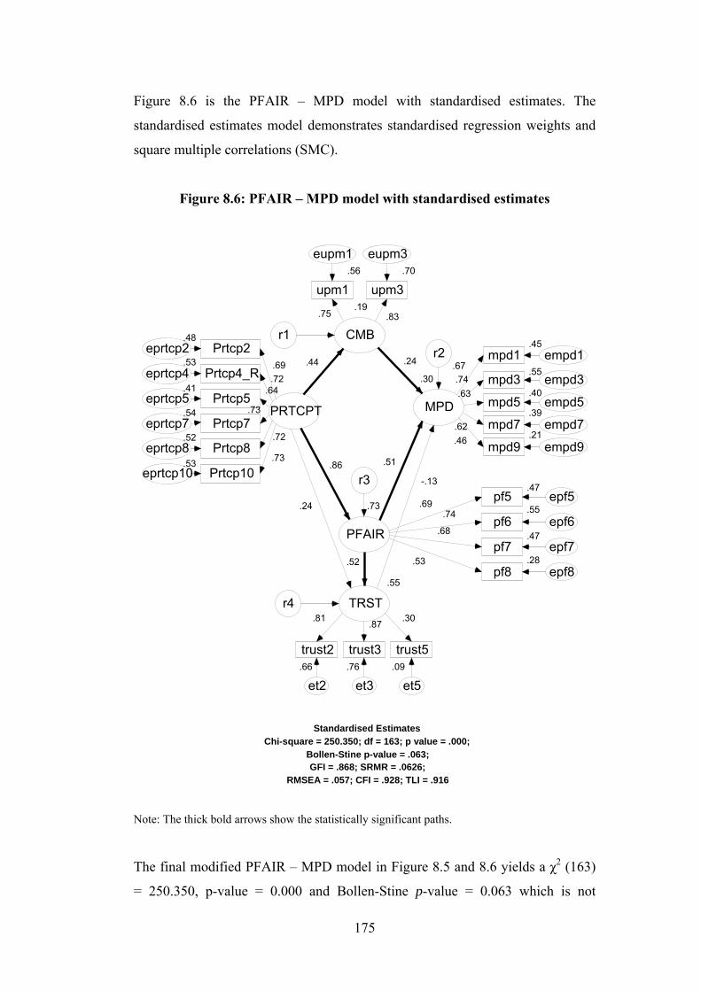
Figure 8.6 is the PFAIR – MPD model with standardised estimates. The

standardised estimates model demonstrates standardised regression weights and

square multiple correlations (SMC).

Figure 8.6: PFAIR – MPD model with standardised estimates

PRTCPT

.53Prtcp10eprtcp10

.73

.52Prtcp8eprtcp8

.72

.54Prtcp7eprtcp7

.73

.41Prtcp5eprtcp5

.64


.48Prtcp2

.69

.19

CMB

.56

upm1

eupm1

.75

.70

upm3

.83

.30

MPD

.45mpd1 empd1

.67 .55mpd3 empd3.74

.40mpd5 empd5

.63

.39mpd7 empd7.62

.21mpd9 empd9.46

.73

PFAIR

.47pf5 epf5.69 .55pf6 epf6

.74

.47pf7 epf7

.68

.28pf8

.53

.55

TRST

.09

trust5

et5

.30

.76

trust3

et3

.87

.66

trust2

et2

.81

r1

.44r2

.24

r3.86

.24

.52

.51

-.13

r4

epf8

eupm3

eprtcp2



RMSEA = .057; CFI = .928; TLI = .916

Note: The thick bold arrows show the statistically significant paths. The final modified PFAIR – MPD model in Figure 8.5 and 8.6 yields a χ2 (163)

= 250.350, p-value = 0.000 and Bollen-Stine p-value = 0.063 which is not

175

significant at the level of 0.05. This is an indication that the model fits the data

very well. After the deletion of item mpd2, there are still four pairs of indicators

(i.e., upm1 – trust2, upm3 – trust3, upm1 – trust3 and upm1 – pf7) that have an

absolute value of standardised residual covariance greater than 2 (see Table 3 in

Appendix III – Part A). This suggests the existence of multi-collinearity. Thus,

one or all of those items should be deleted. However, since the model fits the

data well as indicated by the non-significant Bollen-Stine p-value, those items

are maintained in this model.

The chi-square test (χ2) and the associated p-value is the most common and basic

measures to evaluate a model’s fit (Cunningham, 2008; Kline, 2005). However,

it alone should not be used as a test of validity of a model (Hair, Anderson,

Tatham, Black, 1998) since it loses validity for large samples. Since, no single

measure is proven as the best measure; the present thesis also reporting the other

measures. From Figures 8.5 and 8.6, it can be seen that the other fit measures

also indicate the goodness of fit of the model to the data (GFI = 0.868, SRMR =

0.0626, RMSEA = 0.057, CFI = 0.928 and TLI = 0.916) (see Table 7.2 Chapter 7

for the reference of the fit measures).

The final modified model shows all paths; however, only five paths between the

exogenous variable and the endogenous variables are statistically significant at

the 0.01 and 0.05 level of significance (see regression weights estimates of

significant paths in Table 8.1).

Table 8.1 Regression weights for PFAIR – MPD model

Ho Number Estimate S.E. C.R. p-value

H2a PFAIR <--- PRTCPT 1.004 .136 7.387 *** H4 TRST <--- PRTCPT .132 .118 1.118 .264 H8a TRST <--- PFAIR .242 .120 2.015 .044** H1 CMB <--- PRTCPT .500 .124 4.049 *** H5a MPD <--- CMB .150 .067 2.255 .024** H6a MPD <--- PFAIR .317 .109 2.892 .004*** H7a MPD <--- TRST -.175 .216 -.813 .416

Note: *** p-value is statistically significant at the 0.01 level (two-tailed) ** p-value is statistically significant at the 0.05 level (two-tailed)

176

The final modified model also indicates that there are varying explanations for

the dependent variables. The square multiple correlations of a variable show the

proportion of its variance that is accounted for by its predictors (determinants)

(Arbuckle, 2006a). As illustrates in Table 8.2, determinant participation

(PRTCPT) accounts for the variance of dependent variables, with a high degree

of explanation for procedural fairness (PFAIR) and trust (TRST), and a

reasonable explanation for use of performance measure (CMB) and managerial

performance (MPD). Specifically, the determinant accounts for:

• 73.5% of the variance of PFAIR;

• 54.9% of the variance of TRST;

• 18.9% of the variance of CMB; and

• 30.4% of the variance of MPD.

Table 8.2 Squared multiple correlations (SMC) for PFAIR – MPD model

Estimate PFAIR .735 TRST .549 CMB .189 MPD .304

The standardised regression weights are also used since they allow the direct

comparison of the relative effect of each independent variable on the dependent

variable (Hair et al., 2006).

Five research hypotheses between the determinant and dependent variables in the

PFAIR – MPD model are accepted. They are: H1; H2a; H5a; H6a; and H8a,

while H4 and H7a are rejected. This suggests that PRTCPT PFAIR, PRTCPT

CMB, PFAIR TRST, PFAIR MPD, and CMB MPD. Hence, it can

be said that participation in the development of performance measures

significantly influences procedural fairness and common-measure bias.

Concurrently, procedural fairness significantly influences trust between parties in

the performance evaluation process and division’s managerial performance.

Furthermore, common-measure bias significantly influences a division’s

177

managerial performance. However, the results also suggest that participation in

the development of performance measures does not directly significantly

influences the trust between parties involved in the performance evaluation

process. Additionally, trust does not appear to influence significantly division


The relative effect (standardised regression weights) between independent and

dependent variables shows stronger paths (with statistical significance) between

PRTCPT and PFAIR (0.857), PFAIR and TRST (0.522), PFAIR and MPD

(0.507), PRTCPT and CMB (0.435) and CMB and MPD (0.236). The rest are

rather weaker with non-statistical significance (see Table 8.3).

Table 8.3 Standardised regression weights for PFAIR – MPD model

Estimate PFAIR <--- PRTCPT .857TRST <--- PRTCPT .243TRST <--- PFAIR .522CMB <--- PRTCPT .435MPD <--- CMB .236MPD <--- PFAIR .507MPD <--- TRST -.130

This may suggest that the higher the level of participation in developing the

performance measures, the greater the procedural fairness perception of the

performance measures and the lower the common-measure bias. Moreover, this

also suggests that the greater the procedural fairness perception of the

performance measures, the stronger the trust between parties involved in the

evaluation process. Finally, a significant positive influence on division

managerial performance occurs when procedural fairness level is high and the

common-measure bias is low.

Furthermore, from the paths diagram (see Figures 8.5 and 8.6), it can be seen that

the participation in developing the performance measures does not have a

significant direct impact on the trust between parties involved in the evaluation

178

process. However, participation significantly influences the trust via procedural

fairness. This suggests that procedural fairness mediates the relationship between

the participation in developing the performance measures and the trust between

parties involved in the performance evaluation process.

A mediator variable is a third variable that influences the relationship between

the independent and dependent variable. It does this in such way that the direct

relationship between the independent and dependent variable is no longer

significant after its introduction (Baron and Kenny, 1986; Holmbeck, 1997). The

relationship between the participation in developing the performance measures

(PRTCPT) and the trust between parties involved in the performance evaluation

process (TRST) is no longer significant when the relationship has been

controlled with the procedural fairness variable (PFAIR). Therefore, procedural

fairness is acting as a mediator variable. The complete examination of the

mediator variable is presented in the sub-section 8.5.1.1.

8.5.1.1 Mediator Variable

A mediator variable is a third variable that accounts for the relationship between

the independent variable and dependent variable (Baron and Kenny, 1986;

Holmbeck, 1997). To test a potential mediator variable, assume B is the

hypothesised mediator between A and C. There are four conditions that must be

satisfied (Cunningham, 2008), as follows.

1. A is significantly associated with C;

2. A is significantly associated with B;

3. B is significantly associated with C; and

4. The direct impact of A on C is reduced (i.e., no longer significant) after

controlling for the mediator B.

To test whether procedural fairness (PFAIR) mediates the relationship between

participation in the developing performance measures (PRTCPT) and trust

between parties involved in the performance evaluation process (TRST), the

paths analysis of the three variables are examined. The initial model that

illustrated the direct relations between PRTCPT and TRST, with the

179

unstandardised and standardised estimates, is presented in Figures 8.7 and 8.8

respectively.

Figure 8.7: Unstandardised initial model of PRTCPT and TRST

.39

PRTCPT

Prtcp10.33

eprtcp10 1.001

Prtcp8.36

eprtcp8.981

Prtcp7.41

eprtcp71.12

Prtcp5.58

eprtcp5 .991Prtcp4_R

.36eprtcp4 1.05

1Prtcp2

.41eprtcp2

.95

1

TRST

trust2 .33

et21.001

trust3 .20et31.22 1

trust5 1.15.44

1 .29

r1

1

Unstandardised Estimates

1.79

Chi-square = 49.183; df = 26; p value = .004;Bollen-Stine p-value = .090;GFI = .934; SRMR = .0467;

RMSEA = .074; CFI = .959; TLI = .944

et5


Figure 8.8: Standardised initial model of PRTCPT and TRST

.39

PRTCPT

Prtcp10.33

eprtcp101.001

Prtcp8.36

eprtcp8.981

Prtcp7.41

eprtcp71.12

Prtcp5.58

eprtcp5.991

Prtcp4_R.36

eprtcp4 1.051

Prtcp2.41

eprtcp2.95

1

TRST.79

1

.291

r1

trust2 .33

et21.001

trust3 .20et31.22 1

trust5 1.15et5.441



RMSEA = .074; CFI = .959; TLI = .944

Note: The thick bold arrows show the statistically significant paths. The initial PRTCPT - TRST model in Figures 8.7 and 8.8 yields a χ2 (26) =

49.183, p-value = 0.004, and Bollen-Stine p-value = 0.090 which is not

180

181


very well. The other fit measures also indicate the goodness of fit of the model to

the data (GFI = 0.934, SRMR = 0.0467, RMSEA = 0.074, CFI = 0.959, TLI =

0.944) (see Table 7.2 Chapter 7 for the reference of the fit measures).

The initial model shows the path between PRTCPT and TRST is statistically

significant at the 0.01 level of significance (see regression weights estimates of

significant path in Table 8.4). Table 8.5 shows that determinant (PRTCPT)

accounts for the variance of TRST with a high degree of explanation (45.5%).

The standardised regression weights (see Table 8.6) show the strong effect

between PRTCPT and TRST (0.675). This suggests that participation in

developing performance measures directly impacts trust the between parties

involved in the performance evaluation process.

Table 8.4 Regression weights of initial model of PRTCPT – TRST Estimate S.E. C.R. p-value

TRST <--- PRTCPT .792 .122 6.475 *** Note: *** p-value is statistically significant at the 0.01 level (two-tailed)

Table 8.5 Squared multiple correlations of initial model of PRTCPT - TRST

Estimate TRST .455

Table 8.6 Standardised regression weights of initial model of PRTCPT - TRST

Estimate TRST <--- PRTCPT .675

The paths diagram, when introducing the procedural fairness (PFAIR) variable,

is presented below with unstandardised estimates and standardised estimates in

Figures 8.9 and 8.10 respectively.

Figure 8.9: Unstandardised mediating model of PRTCPT - TRST


Figure 8.10: Standardised mediating model of PRTCPT – TRST

.39

PRTCPT

Prtcp10.33

eprtcp101.001

Prtcp8.35

eprtcp81.001

Prtcp7.41

eprtcp71.12

Prtcp5.57

eprtcp51.021

Prtcp4_R.37

eprtcp4 1.041

Prtcp2.40

eprtcp2.96

1

PFAIR

pf8.65

epf8

1pf7

.32

epf7

1.00

1pf6

.30

epf6

1.29

1pf5

.58

epf5

1.45

1

.31TRST

trust2 .29

et21.001

r1

1

trust3 .25

et31.15 1

trust5 1.14

et5.451

.08

r21

.67 .76



RMSEA = .059; CFI = .959; TLI = .948

1

1.00

PRTCPT

.54Prtcp10eprtcp10

.73

.52Prtcp8eprtcp8

.72

.54Prtcp7eprtcp7

.74

.42Prtcp5eprtcp5

.65


.47Prtcp2

.69

.68

PFAIR

.28

pf8

epf8.45

pf7

epf7

.67

.59

pf6

epf6

.77

.49

pf5

epf5

.70

.54

TRST.66trust2 et2.81

.76trust3 et3.87

.09trust5.30

r2

.82 .51

.53

.26

r1

et5

eprtcp2

.26



RMSEA = .059; CFI = .959; TLI = .948


182

The mediating PRTCPT - TRST model in Figures 8.9 and 8.10 yields a χ2 (62) =

97.208, p-value = 0.003, and Bollen-Stine p-value = 0.160 which is not


very well. The other fit measures also indicate the goodness of fit of the model to

the data (GFI = 0.916, SRMR = 0.0474, RMSEA = 0.059, CFI = 0.959, TLI =

0.948) (see Table 7.2 Chapter 7 for the reference of the fit measures).

The mediating model shows that the path between PRTCPT and PFAIR is

statistically significant at the 0.01 level of significance. The path between PFAIR

and TRST is also statistically significant at the 0.05 level of significance.

However, the path between PRTCPT and TRST is no longer statistically

significant (see regression weights estimates of significant path in Table 8.7).

Table 8.8 shows that the determinant (PRTCPT) accounts for the variance of

dependent variables with a high degree of explanation for PFAIR and TRST. The

determinant accounts for:

• 67.6% of the variance of PFAIR; and

• 54.0% of the variance of TRST

Table 8.7 Regression weights of mediating model of PRTCPT – TRST

Estimate S.E. C.R. p-value PFAIR <--- PRTCPT .671 .116 5.807 *** TRST <--- PFAIR .757 .288 2.630 .009*** TRST <--- PRTCPT .312 .213 1.463 .143

Note: *** p-value is statistically significant at the 0.01 level (two-tailed)

Table 8.8 Squared multiple correlations of mediating model of PRTCPT - TRST

Estimate PFAIR .676 TRST .540

183

184

Table 8.9 Standardised regression weights of mediating model of PRTCPT - TRST

Estimate PFAIR <--- PRTCPT .822TRST <--- PFAIR .509TRST <--- PRTCPT .257



PRTCPT and PFAIR (0.822) and PFAIR and TRST (0.509). The path between

PRTCPT and TRST is rather weaker with no-statistical significance (see Table

8.9).

From the analysis of the initial and mediating model above, it can be inferred that

PFAIR mediates the relationship between PRTCPT and TRST, since the four

conditions for a mediator variable have been satisfied. This suggests that

participation in developing performance measures impacts the trust between the

parties involved in the performance evaluation process, via procedural fairness of

the development of the performance measures.

8.5.2 Procedural Fairness (PFAIR) – MPS Model The initial PFAIR – MPS model, prior to any modification, comprises

unstandardised estimates and is presented in Figure 8.11 while the standardised


Figure 8.11: Initial PFAIR – MPS model with unstandardised estimates

.38PRTCPT

Prtcp10.34

eprtcp101.001

Prtcp8.36

eprtcp81.001

Prtcp7.41

eprtcp71.131

Prtcp5.57


.37eprtcp4 1.05

1Prtcp2

.40

eprtcp2.97

1 CMB

upm1

.50

eupm1

1.00

1

upm3

.13

eupm3

1.48

1

MPS

mps1.33

emps1.901

mps2.24

emps21.00 1

mps3.19

emps31.001

PFAIR

pf5.58

epf51.00

1

pf6.30

epf6.90 1

pf7.32

epf7.69 1

pf8.66

epf8.69 1

TRST

trust51.14

et5

1.00

1trust3

.24

et3

2.62

1trust2

.30

et2

2.26

1

.34

r11 .92

r21

.17

r31

.05

r41

.98 .15

.21



RMSEA = .066; CFI = .936; TLI = .924

.40 .77

.26

.16

185

Figure 8.12: Initial PFAIR – MPS model with standardised estimates

PRTCPT

.53Prtcp10eprtcp10

.73

.52Prtcp8eprtcp8

.72

.54Prtcp7eprtcp7

.74



.47Prtcp2eprtcp2

.69

.15

CMB

.45

upm1

eupm1

.67

.87

upm3

eupm3

.94

.26

MPS

.76mps1 emps1.87

.84mps2 emps2.91

.87mps3 emps3.93

.69

PFAIR

.48pf5 epf5

.69 .59pf6 epf6.77

.45pf7 epf7

.67

.28pf8 epf8

.53

.55

TRST

.09

trust5

et5

.30

.76

trust3

et3

.87

.65

trust2

et2

.81

r1r2

r3

r4

.83 .10

.47



RMSEA = .066; CFI = .936; TLI = .924

.39 .44

.08

.31

From Figures 8.11 and 8.12 above, it can be seen that the initial PFAIR – MPS

model does not fit the data well as indicated by the significant chi-square fit, χ2

(128) = 220.163, p-value = 0.000 and Bollen-Stine p-value = 0.042. The

structural modelling of data requires that the data and the model being tested are

not significantly different or p-value is greater than 0.05. Additionally, with the

186

187

multi-variate non-normality data, the Bollen-Stine p-value will be applied. In

order to accept the model, the Bollen-Stine p-value should be greater than 0.05.

Hence, the model needs to be re-specified to better fit the data. The process of re-

specifying the model is conducted by an examination of the standardised residual

covariance matrix (SRMC) and modification indices (MIs). In the examination of

the SRMC and MIs (see Table 1 and 2 in Appendix III – Part B), it is found that

there are four pairs (i.e., upm1 – trust2, upm3 – trust3, upm1 – trust3 and upm1 –

pf7) of indicators that have an absolute value of standardised residual covariance

greater than 2. This indicates that this particular covariance is not well

reproduced by the hypothesised model (Cunningham, 2008). Therefore, one or

all of the items should be deleted.

The information obtained from the assessment of the MIs is consistent with that

obtained from the assessment of the SRMC. The MIs indicate that deleting item

pf7 would result in a decrease of the χ2 statistic of at least 9.156 for a reduction

of df of 1. After this deletion, the model fits the data very well (see Figure 8.13

and 8.14).

Figure 8.13 is the PFAIR – MPS model after re-specification with the

unstandardised estimates. The unstandardised estimates model demonstrates


Figure 8.13: PFAIR – MPS model with unstandardised estimates

.38

PRTCPT

Prtcp10.34

eprtcp101.001

Prtcp8.36

eprtcp8.991

Prtcp7.41

eprtcp71.141

Prtcp5.57

eprtcp51.021

Prtcp4_R.37

eprtcp4 1.061

Prtcp2.41

eprtcp2.96

1 CMB

upm1

.50

eupm1

1.00

1

upm3

.11

.39

eupm3

1.50

1

.78

MPS

mps1

r21

.341 .92r1

.33emps1.90

1

mps2.25

emps21.00 1

mps3.19

emps31.001

PFAIR

pf5.56

epf51.001

pf6.26

epf6.92 1

pf8.68

epf8.641

TRST

trust51.14

et5

1.00

1trust3

.22

et3

2.65

1trust2

.31

et2

2.22

1

.20

r31

.05

r41

.97 .19

.18

.20

.20



RMSEA = .061; CFI = .950; TLI = .939


188

Figure 8.14 is the PFAIR – MPS model with standardised estimates. The

standardised estimates model illustrates standardised regression weights and

square multiple correlations (SMC).

Figure 8.14: PFAIR – MPS model with standardised estimates

PRTCPT

.53Prtcp10eprtcp10

.73

.51Prtcp8eprtcp8

.71

.55Prtcp7eprtcp7

.74

.41Prtcp5eprtcp5

.64


.46Prtcp2

.68

.14

CMB

.44

upm1

eupm1

.67

.89

upm3

eupm3

.94

.27

MPS

.76 mps1 emps1.87

.84 mps2 emps2

.91

.87 mps3 emps3.93

.64

PFAIR

.50 pf5 epf5.71

.64 pf6 epf6

.80

.25 pf8.50

.54

TRST

.09

trust5

et5

.30

.78

trust3

et3

.88

.64

trust2

et2

.80

r1

.38r2

.44

.13

.06r3.80

.41

.36

r4

epf8

eprtcp2



RMSEA = .061; CFI = .950; TLI = .939


The modified PFAIR – MPS model in Figures 8.13 and 8.14 yields a χ2 (112) =

179.933, p-value = 0.000 and Bollen-Stine p-value = 0.092 which is not

189

190


very well. This suggests that there is no difference between the model and the

data.

However, after the deletion of item pf7, the three pairs (i.e., upm1 – trust2, upm3

– trust3 and upm1 – trust3) of indicators still have an absolute value of

standardised residual covariance greater than 2 (see Table 3 in Appendix III –

Part B). Additionally, the standardised residual covariance of items upm1 – pf8 is

also greater than 2. This is an indication of the existence of multi-collinearity.

Therefore, one or all of the items should be dropped. However, since the model

fits the data well, that is, that there is no difference between the model and the

data, those items are maintained in this model.

Based on the non-significant Bollen-Stine p-value of 0.092 at a level of 0.05, it

can be seen that the model fits the data well; however it is necessary to check the

other fit measurements, since no single measure has proven to be the best

measure. Fortunately, based on Figures 8.13 and 8.14, the other fit measures also

indicate the satisfactory fit of the model to the data (GFI = 0.883, SRMR =

0.0591, RMSEA = 0.061, and CFI = 0.950, TLI = 0.939) (see Table 7.2 Chapter

7 for the reference of the fit measures).

The modified model shows all paths, however, only four paths between the

exogenous variable and endogenous variables are significant at the 0.01 and 0.05

level of significance (see regression weights estimates of significant paths in

Table 8.10).

Table 8.10 Regression weights for PFAIR – MPS model Ho Number Estimate S.E. C.R. p-value

H2a PFAIR <--- PRTCPT .968 .138 7.026 *** H8a TRST <--- PFAIR .184 .092 2.007 .045** H1 CMB <--- PRTCPT .385 .108 3.563 *** H4 TRST <--- PRTCPT .195 .103 1.889 .059

H6b MPS <--- PFAIR .192 .204 .944 .345 H5b MPS <--- CMB .775 .160 4.854 *** H7b MPS <--- TRST .201 .435 .461 .645


The new modified model also indicates that there are varying explanations for

the dependent variables. Table 8.11 demonstrates that determinant (PRTCPT)

accounts for the variance of dependent variables with a high degree of

explanation for procedural fairness (PFAIR) and trust (TRST), and a reasonable

explanation for the use of performance measures (CMB) and managerial

performance based on division manager’s view of senior manager’s perception of

performance (MPS). Specifically, the determinant accounts for:

• 64.3% of the variance of PFAIR;


• 14.2% of the variance of CMB; and

• 26.9% of the variance of MPS.

Table 8.11 Squared multiple correlations (SMC) for PFAIR – MPS model

Estimate PFAIR .643 TRST .539 CMB .142 MPS .269

In the PFAIR – MPS model, one research hypothesis between independent and

dependent variable is accepted, which is H5b, while H6b and H7b are rejected.

This suggests that CMB MPS. Hence, it can be said that common-measure

bias significantly influences division’s managerial performance based on a

division manager’s view of senior manager’s perception of performance.

However, it also found that procedural fairness in the development of

191

192


performance based on division manager’s view of senior manager’s perception.

Likewise with trust, which also does not significantly influence the division’s

managerial performance (senior manager’s self-assessment).



PRTCPT and PFAIR (0.802), CMB and MPS (0.437), PFAIR and TRST (0.412),

PRTCPT and CMB (0.377) and PRTCPT and TRST (0.361). The rest are rather

weaker and not statistically significant (see Table 8.12). Table 8.12 Standardised regression weights for PFAIR – MPS model

Estimate PFAIR <--- PRTCPT .802TRST <--- PFAIR .412CMB <--- PRTCPT .377TRST <--- PRTCPT .361MPS <--- PFAIR .128MPS <--- CMB .437MPS <--- TRST .060


performance measures, the greater the procedural fairness perception of the


also suggests that the greater the procedural fairness perception of the


performance evaluation process. Finally, a significant positive influence on

division’s managerial performance, based on division manager’s view of senior

manager’s perception of performance, occurs when common-measure bias level

is low.

8.6 Distributive Fairness Model With the investigation of the procedural fairness model, the examination of the

distributive fairness model using SEM’s path data analysis are also divided into

two models, which are DFAIR – MPD and DFAIR – MPS model.

8.6.1 Distributive Fairness (DFAIR) – MPD Model The initial DFAIR – MPD model, prior to any modification, comprises of

unstandardised estimates and is presented in Figure 8.15, while the standardised


Figure 8.15: Initial DFAIR – MPD model with unstandardised estimates

.39

PRTCPT

Prtcp10.34

eprtcp101.001

Prtcp8.36

eprtcp8.991

Prtcp7.44

eprtcp71.10

Prtcp5.56


.38

eprtcp4 1.031

Prtcp2.38

eprtcp21.00

1 CMB

upm1

.40

eupm1

1.00

1

upm3

.29

eupm3

1.21

1

MPD

mpd1.26

empd11.00

1

mpd2.42

empd2.741

mpd3.24

empd31.26 1

mpd5.33

empd5.95

1

mpd7.51

empd71.311

DFAIRdf1

.30

edf11.10 1

df2.53

edf21.001

TRST

trust51.13

et5

1.00

1trust3

.26

et3

2.47

1trust2

.29

et2

2.17

1

.41

r11 .13

r21

.06

r31

.01

r41

.73

-.36

1.02



RMSEA = .064; CFI = .914; TLI = .898

.49 .12

1.03

-1.11

1

mpd9.32

empd9.68 1

193

Figure 8.16: Initial DFAIR – MPD model with standardised estimates

PRTCPT

.53Prtcp10eprtcp10

.73

.51Prtcp8eprtcp8

.71

.52Prtcp7eprtcp7

.72



.50Prtcp2eprtcp2

.71

.18

CMB

.55

upm1

eupm1

.74

.72

upm3

eupm3

.85

.36

MPD

.44mpd1 empd1

.66 .21mpd2 empd2.46.57

mpd3 empd3.76.36

mpd5 empd5.60 .41mpd7 empd7.64

.79

DFAIR

.52df1 edf1.72

.33df2 edf2.58

.95

TRST

.10

trust5

et5

.31

.74

trust3

et3

.86

.66

trust2

et2

.81

r1r2

r3

r4

.89

-.64

1.50



RMSEA = .064; CFI = .914; TLI = .898

.43 .20

1.18

-.86

.23mpd9 empd9

.48

It can be seen in Figures 8.15 and 8.16 above, that the initial model does not fit

well with the data, since the chi-square fit, χ2 (145) = 242.768, p-value = 0.000

and Bollen-Stine p-value = 0.008 which is significant at 0.05 level of

significance. Since the structural modelling requires that the data, and the model

being tested, are not significantly different or have a p-value that is greater than

0.05, the model needs to be re-specified to fit better. Furthermore, given that

there are multi-variate non-normality data, the Bollen-Stine p-value will be used.

194

195

This Bollen-Stine p-value should be greater than 0.05 in order to accept the

model. The re-specification of the model will be done by the examination of the

standardised residual covariance (SRMC) and modification indices (MIs). The

assessment of the SRMC and MIs (see Table 1 and 2 in Appendix III – Part C),

found that three pairs (i.e., upm1 – trust2, upm3 – trust3 and upm1 – trust3) of

indicators have an absolute value of standardised residual covariance greater than

2. This suggests that a particular covariance is not well reproduced by the

hypothesised model (Cunningham, 2008). Therefore, one or all of the indicators

should be deleted.

The inspection of the MIs is also providing consistent results with those obtained

from the inspection of the SRMC. For example, the MIs indicate that deleting

item upm1 would result in a decrease of the χ2 statistic of at least 5.681 for a

reduction in df of 1. Given that, it seems reasonable to delete item upm1. This

process would be repeated until the model represents a good fit to the data. After

this deletion, the model fits the data very well (see Figures 8.17 and 8.18).

Figure 8.17 is the DFAIR – MPD model after re-specification with the

unstandardised estimates. The unstandardised estimates model shows regression

weights and variances.

Figure 8.17: DFAIR – MPD model with unstandardised estimates

.82

.39PRTCPT

Prtcp10.33

eprtcp10 1.001

Prtcp8.37

eprtcp8.981

Prtcp7.44

eprtcp71.09

Prtcp5.57

1eprtcp5

1.021Prtcp4_R

.38

eprtcp4 1.03

1Prtcp2

.38

1.00

1 CMB

upm3

eupm31

1.00

.86.58

.08

.081

r1

MPD

mpd1.27

empd11.00

1

mpd2.42

empd2.751

1mpd3

.23

empd31.27

1

r2

mpd5.32

empd5.97

mpd7.51

empd71.331

DFAIRdf1

.21

edf11.10 1

df2.46

edf21.001

TRST

trust51.14

et5

1.00

1trust3

.24

et3

2.55

1trust2

2.21

.14

r31

.04

r41

.71

.10

.39

-.12

-.05

.69 .321

empd9mpd9

.30

et2

1

1

eprtcp2



RMSEA = .056; CFI = .937; TLI = .925


196

Figure 8.18 is the DFAIR – MPD model with standardised estimates. The

standardised estimates model demonstrates standardised regression weights and

SMC.

Figure 8.18: DFAIR – MPD model with standardised estimates

PRTCPT

.54Prtcp10eprtcp10

.73

.50Prtcp8eprtcp8

.71

.52Prtcp7eprtcp7

.72

.42Prtcp5eprtcp5

.65


.51Prtcp2

.71 .63

.20

upm3.45

eupm3

CMB

.60

MPD

.43 mpd1 empd1

.65 .21 mpd2 empd2.46

.58 mpd3 empd3.76

.36 mpd5 empd5.60 .41 mpd7 empd7.64

.23 mpd9

.48empd9

.59

DFAIR

.66 df1 edf1.81

.42 df2.65

.65

TRST

.09trust5

et5

.31

.76trust3

et3

.87

.66trust2

et2

.81

r1

.80r2

.88

r3.77

.18

.66

-.16

-.04

r4

edf2

eprtcp2



RMSEA = .056; CFI = .937; TLI = .925


The final modified DFAIR – MPD model in Figures 8.17 and 8.18 yields a χ2

(128) = 192.805, p-value = 0.000 and Bollen-Stine p-value = 0.076 which is not


197

very well. After the deletion of item upm1, there is still one pair of indicators

which is upm3 – trust3 that have an absolute value of standardised residual

covariance greater than 2 (see Table 3 in Appendix III – Part C). This is an

indication of the existence of multi-collinearity. Therefore, one or both, of those

items should be deleted. However since the model fits the data well, as indicated

by the not significant Bollen-Stine p-value, those items are maintained in this

model.

As can be seen in Figures 8.17 and 8.18, the non-significant Bollen-Stine p-value

of 0.076 at a level of 0.05 indicates that the model fits the data well. However,

since no single measure is the best measure of fit, it is necessary to examine other

model fit measures. Based on Figures 8.17 and 8.18, the other fit measures also

indicate the satisfactory fits of the model to the data (GFI = 0.886, SRMR =

0.0572, RMSEA = 0.056, CFI = 0.937 and TLI = 0.925) (see Table 7.2 Chapter 7

for the reference of the fit measures).

The final modified model shows all paths, however, only four paths between the

exogenous variable and endogenous variables are statistically significant at the

0.01 level of significance. This is shown in the regression weights estimates of

significance in Table 8.13.

Table 8.13 Regression weights for DFAIR – MPD model Ho Number Estimate S.E. C.R. p-value

H2b DFAIR <--- PRTCPT .715 .113 6.315 *** H4 TRST <--- PRTCPT .098 .096 1.026 .305

H8b TRST <--- DFAIR .390 .151 2.583 .010*** H1 CMB <--- PRTCPT .577 .135 4.291 *** H5a MPD <--- CMB .861 .282 3.051 .002*** H6c MPD <--- DFAIR -.119 .192 -.621 .534 H7a MPD <--- TRST -.051 .245 -.208 .835

Note: *** p-value is statistically significant at the 0.01 level (two-tailed)

The final modified model also indicates that there are varying explanations for

the dependent variables. Table 8.14 shows that determinant (PRTCPT) accounts

for the variance of the dependent variables with a high degree of explanation for

DFAIR, CMB, TRST and MPD. Specifically, the determinant accounts for:

• 59.5% of the variance of DFAIR;

• 63.4% of the variance of CMB;

198

• 64.9% of the variance of TRST; and

• 60.0% of the variance of MPD. Table 8.14 Squared multiple correlations (SMC) for DFAIR – MPD model

Estimate DFAIR .595 CMB .634 TRST .649 MPD .600

The results indicate that four research hypotheses between the determinant and

dependent variables in the DFAIR – MPD model are accepted. They are: H1;

H2b; H5a; and H8b, while H4, H6c and H7a are rejected. This suggests that

PRTCPT DFAIR, PRTCPT CMB, DFAIR TRST, and CMB MPD. It

can be said that participation significantly influences distributive fairness and

common-measure bias. Simultaneously, distributive fairness significantly

influences trust between the parties involved in the performance evaluation

process. In addition, common-measure bias significantly influences the division’s

managerial performance. However, the results also suggest that participation in

the development of performance measures does not directly significantly

influence the trust between parties involved in the performance evaluation

process. Furthermore, both trust and distributive fairness did not significantly

influence the division’s managerial performance.



PRTCPT and DFAIR (0.771), DFAIR and TRST (0.659), PRTCPT and CMB

(0.796) and CMB and MPD (0.877). The rest are rather weaker with non-

statistical significance (see Table 8.15).

199

200

Table 8.15 Standardised regression weights for DFAIR – MPD model

Estimate DFAIR <--- PRTCPT .771TRST <--- PRTCPT .179TRST <--- DFAIR .659CMB <--- PRTCPT .796MPD <--- CMB .877MPD <--- DFAIR -.155MPD <--- TRST -.039

This suggests that the higher the level of participation in developing the

performance measures, the greater the distributive fairness perception of the


also suggests that the greater the distributive fairness perception of the


performance evaluation process. Finally, the lower the common-measure bias,

the better the division’s managerial performance.

Additionally, from the paths diagram (see Figure 8.17 and 8.18), it can be seen

that participation in developing the performance measures does not have a

significant direct impact in the trust between parties involved in the evaluation

process. However, participation significantly influences the trust via distributive

fairness. This implies that distributive fairness mediates the relationship between

the participation in developing the performance measures, and the trust between

parties involved in the performance evaluation process.

8.6.2 Distributive Fairness (DFAIR) – MPS Model The initial DFAIR – MPS model, prior to any modification, is presented in

Figure 8.19 with unstandardised estimates and in Figure 8.20 with standardised

estimates.

Figure 8.19: Initial DFAIR – MPS model with unstandardised estimates

.38PRTCPT

Prtcp10.34

eprtcp101.001

Prtcp8.36

eprtcp8.991

Prtcp7.43

eprtcp71.11

Prtcp5.57


.38

eprtcp4 1.041

Prtcp2.39

eprtcp2.99

1 CMB

upm1

.49

eupm1

1.00

1

upm3

.13

eupm3

1.48

1

MPSmps1

.33emps1.90 1

mps2.24

emps21.00

1

mps3.20

emps31.001

DFAIRdf1

.21

edf11.10 1

df2.46

edf21.001

TRST

trust51.14

et5

1.00

1trust3

.24

et3

2.57

1trust2

.30

et2

2.21

1

.34

r11 .93

r21

.13

r31

.04

r41

.72

.10

.38



RMSEA = .076; CFI = .931; TLI = .915

.41 .78

.09

.36

1

201

Figure 8.20: Initial DFAIR – MPS model with standardised estimates

PRTCPT

.53Prtcp10eprtcp10

.73

.51Prtcp8eprtcp8

.72

.53Prtcp7eprtcp7

.73



.49Prtcp2eprtcp2

.70

.16

CMB

.45

upm1

eupm1

.67

.87

upm3

eupm3

.93

.26

MPS

.76mps1 emps1.87

.84mps2 emps2.92 .86mps3 emps3.93

.60

DFAIR

.66df1 edf1.81

.42df2 edf2.65

.65

TRST

.09

trust5

et5

.30

.76

trust3

et3

.87

.65

trust2

et2

.81

r1r2

r3

r4

.77

.19

.65



RMSEA = .076; CFI = .931; TLI = .915

.40 .44

.04

.11

From Figures 8.19 and 8.20 above, it can be seen that the initial DFAIR – MPS

model does not fit the data well as indicated by the significant chi-square fit, χ2

(97) = 188.925, p-value = 0.000 and Bollen-Stine p-value = 0.015. The structural

modelling of data requires that the data and the model being tested are not

significantly different or have a p-value that is greater than 0.05. In addition, the

Bollen-Stine p-value will be used because of the multi-variate non-normality of

the data. This needs to have value greater than 0.05 as well.

202

203

Given that, the initial model needs to be re-specified to fit better. This process is

conducted via an examination of the standardised residual covariance matrix

(SRMC) and modification indices (MIs). The examination of SRMC and MIs

(see Table 1 and 2 in Appendix III – Part D) found two pairs (i.e., upm1 – trust2

and upm1 – trust3) of indicators that have an absolute value of standardised

residual covariance greater than 2. This suggests that a particular covariance is

not well reproduced by the hypothesised model (Cunningham, 2008). Therefore,

one or all, of the indicators should be dropped. The inspections of the MIs also

confirmed this result. Based on the information, items upm1 and trust3 have to

be deleted to arrive at a good fit model. Following this deletion, the model fits

the data very well (see Figure 8.21 and 8.22).

Figure 8.21 is the DFAIR – MPS model after re-specification with the

unstandardised estimates. The unstandardised estimates model illustrates


Figure 8.21: DFAIR – MPS model with unstandardised estimates

.58

.39PRTCPT

Prtcp10 .33

eprtcp101.001

Prtcp8.35

eprtcp81.001

Prtcp7.43

eprtcp71.10

Prtcp5.56

eprtcp51

1.031 Prtcp4_R

.39

eprtcp4 1.031

Prtcp2.38

eprtcp2.99

1 CMB

upm3

eupm3

1.00

1

.57 1.281

r2

.311 .59r1

MPSmps1

.32emps1.90 1

mps2.25

emps21.00

1

mps3.19

emps31.001

DFAIRdf1

.20

edf11.12 1

df2.47

1.001

TRST

trust51.11

et5

1.00

1trust2

.17

et2

2.20

1

.13

r31

.07

r41

.71

.04

.45


Bollen-Stine p-value = .149;

-.24

.21

GFI = .912; SRMR = .0492;RMSEA = .060; CFI = .961; TLI = .950

edf2


204

Figure 8.22 is the DFAIR – MPS model with standardised estimates. The

standardised estimates model shows standardised regression weights and SMC.

Figure 8.22: DFAIR – MPS Model with standardised estimates

eupm3


The modified DFAIR – MPS model in Figure 8.21 and 8.22 yields a χ2 (70) =

111.486, p-value = 0.001 and Bollen-Stine p-value = 0.149 which is not

PRTCPT

.54Prtcp10 eprtcp10

.73

.52Prtcp8eprtcp8

.72

.52Prtcp7eprtcp7

.72

.42Prtcp5eprtcp5

.65


.50Prtcp2eprtcp2

.71

.28

CMB

.43

upm3.66

.53

MPS

.76mps1 emps1.87

.83mps2 emps2.91 .87mps3 emps3.93

.59

DFAIR

.67df1 edf1.82

.41df2 edf2.64

.53

TRST

.11

trust5

et5

.34

.80

trust2

et2

.90

r1r2

r3

r4

.77

.06

.68



RMSEA = .060; CFI = .961; TLI = .950

.53 .75

-.12

.07

205


very well. After the deletion of the two items, all of the standardised residual co-

variances were less than two in magnitude (see Table 3 in Appendix III – Part

D).

Due to the absence of a single best measure of fit, the present thesis also reports

the other model fit measures. From Figures 8.21 and 8.22, it can be seen that the

other fit measures also demonstrate the goodness of fit of the model to the data

(GFI = 0.912, SRMR = 0.0492, RMSEA = 0.060, CFI = 0.961 and TLI = 0.950)

(see Table 7.2 chapter 7 for the reference of the fit measures).

The modified model shows all paths, however, only four paths between the

exogenous variable and endogenous variables are significant at the 0.01 and 0.05

levels of significances (see regression weights estimates of significant paths in

Table 8.16).

Table 8.16 Regression weights for DFAIR – MPS model Ho Number Estimate S.E. C.R. p-value

H2b DFAIR <--- PRTCPT .709 .114 6.194 *** H4 TRST <--- PRTCPT .036 .112 .320 .749

H8b TRST <--- DFAIR .450 .199 2.263 .024** H1 CMB <--- PRTCPT .565 .135 4.178 ***

H5b MPS <--- CMB 1.284 .526 2.439 .015** H6d MPS <--- DFAIR -.243 .421 -.577 .564 H7b MPS <--- TRST .214 .431 .496 .620


The new modified model also indicates that there are varying explanations for

the dependent variables. Table 8.17 shows that the determinant (PRTCPT)

accounts for the variance of dependent variables with a high degree of

explanation for distributive fairness (DFAIR), trust (TRST) and managerial


perception of performance (MPS) and a reasonable explanation for the use of

performance measures (CMB).

206

Table 8.17 Squared multiple correlations (SMC) for DFAIR – MPS model

Estimate DFAIR .591 TRST .531 CMB .282 MPS .533

Specifically, the determinant accounts for:

• 59.1% of the variance of DFAIR;


• 53.3% of the variance of MPS; and

• 28.2% of the variance of CMB.

In the DFAIR – MPS model, one research hypothesis between the independent

and dependent variable is accepted, which is H5b, while H6d and H7b are

rejected. This suggests that CMB MPS. Hence, it can be said that common-

measure bias significantly influences the division’s managerial performance

based on the division manager’s view of senior manager’s perception of

performance. However, the results also showed that distributive fairness of

performance measures does not significantly influence division managerial

performance. Similarly, trust between parties involved in the performance

evaluation process does not significantly influence division managerial


perception of performance.

From Table 8.18, it can be seen that the relative effect (standardised regression

weights) between independent and dependent variables shows stronger paths

(with statistical significance) between PRTCPT and DFAIR (0.769), DFAIR and

TRST (0.682), CMB and MPS (0.754) and PRTCPT and CMB (0.531). The rest

are rather weaker and not statistically significant (see Table 8.18).

207

Table 8.18 Standardised regression weights for DFAIR – MPS model

Estimate DFAIR <--- PRTCPT .769TRST <--- PRTCPT .059TRST <--- DFAIR .682CMB <--- PRTCPT .531MPS <--- CMB .754MPS <--- DFAIR -.123MPS <--- TRST .072


performance measures, the greater the distributive fairness perception of the


also suggests that the greater the distributive fairness perception of the


performance evaluation process. In addition, the lower the common-measure bias

the better the division’s managerial performance based on the division manager’s

view of senior manager’s perception of performance.

Furthermore, from the paths diagram (see Figure 8.21 and 8.22), it can be seen

that the participation in developing the performance measures significantly

influences the trust between parties involved in the performance evaluation

process via distributive fairness perception of the performance measures. This

implies that distributive fairness perception of the performance measures

mediates the relationship between the participation in the development of the

performance measures, and the trust between parties involved in the performance

evaluation process.

In summary, it can be said that the determinant/predictor significantly explained

some of the dependent variables. Additionally, its capabilities in explaining the

variance of fairness perception (PFAIR and DFAIR) and trust between parties in

the performance evaluation process (TRST) are stronger than the common-

measure bias (CMB) and the division’s managerial performance (MPD and

MPS) in all of the models. The only exception was the DFAIR – MPD model,

where PRTCPT explained the four dependent variables almost equally.

208

The next step, after examining the entire fairness model, is testing hypothesis H3.

The test will be done using SPSS software to conduct frequency testing and a

chi-square test for goodness of fit. This will test the differences in frequencies

between financial and non-financial measures. The examination is presented

below.

8.7 Fairness of Financial vs. Non-financial Measures In the proposed research model, H3 is formulated as:

H3 : Non-financial measures are perceived to be more fair than financial

measures.

This hypothesis basically tests the divisional manager’s perceptions of financial

and non-financial performance measures that have been used to assess their

managerial performance, in terms of their fairness perception. Table 8.19

illustrates the frequencies of the measures category and Figure 8.23 shows the

bar chart of the measures category.

Table 8.19 Frequencies of the measures category

Frequency Valid Percent

Cumulative Percent

Valid FinFair 68 41.5 41.5 Neutral 58 35.4 76.8 NFinFair 38 23.2 100.0 Total 164 100.0

209

Figure 8.23: The bar chart of the measures category

Per c

ent

Measures Categorical

From Table 8.19 and Figure 8.23, it can be seen that 41.5% of the respondents

perceived that financial measures are fairer than non-financial measures, while

only 23.2% perceived that non-financial measures are fairer than financial

measures. The rest of the respondents (35.4%) did not perceive any differences

between the two measures. The bar chart also shows the same pattern. Therefore,

it can be concluded that H3 – non-financial measures are perceived to be more

fair than financial measures – is rejected since a high proportion of the

respondents perceived financial measures as being fairer than the non-financial

measures.

However, further tests are required to determine if differences in frequencies

exists across response categories. A chi-square test for goodness of fit is

conducted to test the differences. The result from the test is presented in Tables

8.20 and 8.21.

210

Table 8.20 Result output of the type of measures Observed N Expected N Residual FinFair 68 54.7 13.3 Neutral 58 54.7 3.3 NFinFair 38 54.7 -16.7 Total 164

Table 8.21 Result output of the test statistics of the type of measures

Type of measures Chi-Square(a) 8.537 df 2 Asymp. Sig. .014

a 0 cells (.0%) have expected frequencies less than 5. The minimum expected cell frequency is 54.7.

From Tables 8.20 and 8.21, it can be seen that the chi-square value is significant

(p < 0.05). Hence, it can be concluded that there are significant differences in the

frequencies of the division manager’s perception of the fairness of performance

measures between financial measures and non-financial measures, χ2 (2, N = 164)

= 8.537, p < 0.05. This result further supports the conclusion that H3 is rejected,

since the divisional managers perceived that financial performance measures are

fairer than non-financial performance measures.

8.8 Summary First, this chapter began with the examination of the model estimation which

included the discussion of standardised and unstandardised structural (path)

coefficient squared multiple correlations (SMC). Second, the proposed research

model with all the hypotheses being tested was outlined. Third, an introduction to

the full structural model was discussed. Finally, two steps of data analysis were

presented and discussed along with the results of the hypotheses testing.

The first step involved testing the research model by investigating the SEM path

analysis based on four full structural models. These four structural models

comprised of two types of fairness: procedural fairness (PFAIR); and distributive

fairness (DFAIR); and two types of managerial performance: division manager’s

211

self-assessment (MPD); and the division manager’s performance based on the

division manager’s view of senior manager’s perception of performance (MPS).

The second step was to conduct frequencies testing and a chi-square test for

goodness of fit. This assessed differences in frequencies between financial and

non-financial measures in terms of their perceived fairness.

From the hypotheses testing in step one, the present research found that not all of

the hypotheses proposed in the current research were supported. The hypotheses

that were accepted in the present study were H1, H2a, H2b, H5a, H5b, H6a, H8a

and H8b. This suggests that participation in developing the performance

measures significantly influences the use of the performance measure as the

common-measure bias decreases. Moreover, participation was seen to influence

significantly the fairness perception of the performance measures, both in

procedural and distributive fairness. Furthermore, the increase of the fairness

perception, both in procedural and distributive fairness, had a significant positive

effect on trust between parties involved in the performance evaluation process. In

addition, procedural fairness perception of the performance measures was found

to influence significantly division managerial performance.

However, the results of the testing in step one also rejected hypotheses H6b, H6c,

H6d, H7a and H7b. This suggests that distributive fairness perception of the


performance. Similarly, the trust between parties involved in the performance

evaluation process was seen not to influence significantly the division’s

managerial performance. Additionally, H4 was also rejected although it was

supported in the PPFAIR – MPS model. This implies that participating in the

development of the performance measures does not significantly influence the

trust between parties involved in the performance evaluation process. However,

participation does indirectly influence the trust via the fairness perception of the

performance measures. The results of the fairness model are summarised in

Figure 8.24.

212

213

Figure 8.24: The fairness perception model


(CMB)

Fairness:

From the hypotheses testing in step 2, H3 was rejected. This suggests that

divisional managers perceive financial measures as being fairer than non-

financial measures. In the next chapter, the conclusion and suggestions in the

present research will be discussed.


Trust (TRST)

- PFAIR - DFAIR


Chapter 9 Discussions, Conclusions and Suggestions

9.1 Introduction While the previous chapter analysed the results of the study, the objective of the

final chapter is to summarise the findings of the study with emphasis on the

fairness perception model. The current chapter will also assess the implications

of the present research as well as outlining the limitations of the study and

suggestions for further research.

9.2 Key Findings of Demographic Characteristics The demographic characteristics findings comprise of the companies and

divisions, the division’s output, the division managers and their general

perceptions relating to the performance measures. Those key findings are briefly

summarised below.

9.2.1 The Companies and the Divisions The companies and divisions data revealed that the agricultural/mining/

construction industry had the largest proportion of respondents (28.0%). This

was followed by the real estate industry (17.1%) and then the manufacturing

industry (14.0%). The company divisions showed a similar pattern, where the

largest proportional participation occurred in the agricultural/mining/construction

industry (22.6%), the real estate industry (14.0%), followed by the

banking/finance/insurance industry (12.2%). Furthermore, according to the data,

most of the division output is for external consumers (39.6%), although there are

divisions that transfer their output internally (17.1%). This suggests that some of

the divisions are structured specifically to provide products to support other

divisions in the company.

9.2.2 The Division Managers The data show that almost all of the division managers were males (94.5%).

Also, a high proportion of division managers were in the 41-50 age group

214

(47.6%), while 25% were in the 51-60 age group. This suggests that division

managers were most likely to be between 41 and 60 years of age and male. The

evidence also highlights that the largest group of the managers (37.8%) had held

their position for less than 2 years, while another 34.1% had held the position

between 3-5 years. However, the amount of time they have been employed by

the company is spread almost equally in each period group ranging from less

than 2 years to more than 11 years. Moreover, in terms of the number of

employees under the responsibility of the division managers, many of them

(45.1%) have less than 100 employees. This increased gradually to 100-200

employees (22.0%) and 200-500 employees (18.9%). There were 23 division

managers (14.0%) who have more than 500 employees. Hence, in terms of the

number of employees under the division manager’s responsibility, the divisions

participating in this study were quite diverse ranging from relatively small

divisions (less than 100) to large divisions (more than 500).

9.2.3 Divisional Managers’ General Perceptions Regarding Performance Measures

The data revealed that, on average, the divisions did not use different

performance measures to evaluate the division manager as an individual or the

division as an entity. Furthermore, on average (3.1), the respondents agreed that

performance measures affected their motivation while appropriate performance

measures positively influenced their performance. They also strongly agreed that

appropriate performance measures mean they were more likely to try their best to

reach the target being set for the performance measures. From these results, it is

clear that appropriate performance measures are important since they affect the

performance and motivation of managers to achieve their targets.

9.2.4 The Performance Measures The data show that divisions (business units) involved in the current study had

diverse performance measures both in financial and non-financial performance

measures. The financial performance measures that have been more commonly

applied in the divisions comprised of: profit (%); ROI (%); revenue/total assets

(%); and others (e.g., budget performance-cost; EBIT/sales (%); working capital

215

(%); EBIT). For non-financial performance measures, market share (%) is used

to a great extent by the divisions to measure customer performance. Other

customer performance measures are also applied, such as, delivered in-full on-

time (DIFOT), product lines/customer, number of customers. To measure

internal business process performance, the most common measure used by the

divisions was the inventory turnover ratio (%). Other measures that have been

used are: stakeholder management, product quality, TIFR (time injury frequency

rates), LTIFR (lost time injury frequency rates), etc. To ascertain learning and

growth performances, measures such as the number of satisfied employee index,

cost reduction from quality product improvement and investment in new product

support ($) are used by divisions. Other performance measures, such as

development training and employee turnover, are also employed by the divisions.

The diversity of performance measures, either financial or non-financial, reflects

the diversity of the divisions (business units) in the current study. Hence,

performance measures applied in each division (business unit) may depend on

the nature, characteristic and function of the division. This finding is consistent

with Kaplan and Norton (1993, 2001) who argued that each division (business

unit) develops unique measures that best capture their strategy.

9.3 The Fairness Perception Model As mentioned in Chapters 1 and 4, there are five research objectives that

underpin the current thesis. They are as follows.

1 To evaluate the relationship between participation and fairness

perception regarding the divisional/unit performance measures used in a

balanced scorecard (BSC) environment.

2 To examine whether financial or non-financial measures are perceived to

be more fair in a BSC environment.

3 To examine the effect of participation on the development of the

performance measures and the use of performance measures in the


216

4 To examine the relationship between participation and interpersonal trust

between parties involved in the performance evaluation process in a BSC

environment.

5 To investigate the effect of participation, fairness perception, and

interpersonal trust in the development of performance measures, on

divisional/unit managerial performance in a BSC environment.

To achieve the research objectives, a fairness perception model was developed to

guide the present research. This was discussed in Chapter 4. The re-presentation

of the model in a path diagram is again illustrated in Figure 9.1.

Figure 9.1: The proposed research model


(CMB)

Fairness:

Two steps were conducted in order to reach the objectives:

1 investigating the SEM path analysis to fulfil the research objectives,

except for research objective 2; and

2 investigating the frequencies differences between financial and non-

financial measures and the chi-square test for goodness of fit to fulfil

research objective 2.


Trust (TRST)

- PFAIR - DFAIR


217

218

9.3.1 Results of Hypotheses Testing with the Procedural Fairness Model

For procedural fairness, two models were examined: PFAIR – MPD model and

PFAIR – MPS model. It was found that six hypotheses were accepted which

were H1, H2a, H5a, H5b, H6a and H8a, while, H4, H6b, H7a and H7b were

rejected. The summary of the results is presented in Table 9.1.

From Table 9.1, it can be seen that the current research supports the hypothesis

that the higher the level of participation in developing the performance measures

the lower the common-measure bias (H1). This suggests that the common-

measure bias problem, found by Lipe and Salterio (2000) in the BSC

environment, can be potentially overcome by allowing the parties involved in the

performance evaluation process (i.e., division manager and senior manager) to

participate in developing the performance measures that will be used in the

performance evaluation process. The findings of the present research provide

further evidence to support hypothesis 1 (H1). Additionally, this finding enriches

previous methods such as: the divide and conquer strategy (Lipe and Salterio,

2002); justice and assurance (Lipe et al., 2004); disaggregated BSC (Roberts et

al., 2004); linked to strategy (Banker et al., 2004); and introducing training (Dilla

and Steinbart, 2005) in reducing the common-measure bias problem in the BSC

environment.

The acceptance of hypotheses H5a and H5b from the current research provides

evidence that the lower the common-measure bias problem, due to participation

in the development of the performance measures, leads to a better managerial

performance of the divisional/business unit managers (division manager’s self-

assessment), as well as a better managerial performance based on the division

manager’s view of senior manager’s perception of performance.

Furthermore, as presented in Table 9.1, hypothesis H2a is supported. This

suggests that the procedural fairness perception of the performance measure is

positively impacted when there is a higher level of participation in developing

the performance measures. This finding is consistent with prior research (see, for

Table 9.1 Summary of the significant influence of determinants on the procedural fairness model

Ho Number

Hypotheses Exogenous Latent

Variable

Endogenous Latent

Variables

Hypotheses’ Result

Explanation

H1 The higher the level of participation in developing the performance measures, the lower the common-measure bias

PRTCPT CMB Accepted Participation significantly influenced the use of performance measures (reducing common-measure bias problem)

H2a The higher the level of participation in developing the performance measures, the greater the procedural fairness perception of the performance measures

PRTCPT PFAIR Accepted Participation significantly influenced procedural fairness

H4 The higher the level of participation in developing the performance measures, the stronger the trust between parties involved in the evaluation process

PRTCPT TRST Rejected Participation did not significantly influence trust

H5a The lower the common-measure bias, the better the managerial performance of the divisional/unit managers (division manager’s self-assessment)

CMB MPD Accepted Reducing common-measure bias significantly influenced division’s managerial performance

H5b The lower the common-measure bias, the better the managerial performance based on division manager’s view of senior manager’s perception of performance

CMB MPS Accepted Reducing common-measure bias significantly influenced division’s managerial performance based on division manager’s view of senior manager’s perception

H6a The higher the procedural fairness perception of performance measures by divisional/unit managers, the better the managerial performance of the divisional/unit managers (division manager’s self-assessment)

PFAIR MPD Accepted Procedural fairness significantly influenced division’s managerial performance

H6b The higher the procedural fairness perception of performance measures by divisional/unit managers, the better the managerial performance based on division manager’s view of senior manager’s perception of performance

PFAIR MPS Rejected Procedural fairness did not significantly influence division’s managerial performance based on division manager’s view of senior manager’s perception

H7a The stronger the level of trust between parties involved in the performance evaluation process, the better the managerial performance of the divisional/unit managers (division manager’s self-assessment)

TRST MPD Rejected Trust did not significantly influence division’s managerial performance

219

220

Table 9.1 Summary of the significant influence of determinants on the procedural fairness model (continued)

Ho Number


Variable

Endogenous Latent

Variables


Explanation

H7b The stronger the level of trust between parties involved in the performance evaluation process, the better the managerial performance based on division manager’s view of senior manager’s perception of performance

TRST MPS Rejected Trust did not significantly influence division’s managerial performance based on division manager’s view of senior manager’s perception

H8a The higher the procedural fairness perception of performance measures by divisional/unit managers, the stronger the trust between parties involved in the evaluation process

PFAIR TRST Accepted Procedural fairness significantly influenced trust

example, Thibaut and Walker, 1975; Folger, 1977; Greenberg, 1986a, Kanfer et

al., 1987; Paese et al., 1988; Lind and Tyler, 1988; Greenberg, 1990b; Lind et al.,

1990; Tyler, 1990; Tyler and Lind, 1992; Organ and Moorman, 1993; Shapiro,

1993; Korsgaard and Roberson, 1995; Muhammad, 2004) that found that

participation is one of the drivers of procedural fairness perception of the

decision process (i.e., in the current study this refers to the performance

evaluation process). This result leads to a better managerial performance of the

divisional/business unit managers (division manager’s self-assessment). This

finding is also in line with prior research (see, for example, Brownell, 1982;

Dunk, 1989; Folger and Konovsky, 1989; Moorman, 1991; Ross, 1994;

Korsgaard and Roberson, 1995; Lau et al., 1995; Lau and Tan, 1998; Lau and

Lim, 2002a) which found that procedural fairness perception of the decision-

making process results in more positive behaviour in relation to organisational

citizenship behaviour, job attitudes, organisational commitment, low job-related

tension and managerial performance.

However, unlike the managerial performance of the divisional/business unit

manager’s (based on division manager’s self-assessment), which was positively

impacted by the procedural fairness perception of performance measures, the


perception of performance is not positively influenced by the procedural fairness

perception of the performance measures (H6b). This result confirms that there

are complex, rather than simple, relationships that exist between procedural

fairness and performance (Lau and Lim, 2002a). The other explanation of this

result is probably due to the limitation of the current study which only collected

the data from divisional/business unit managers. Hence, an opportunity for

further research may focus on explaining this issue based on the senior

manager’s viewpoint.

Moreover, this current research also found that the higher the procedural fairness

perception of performance measures by divisional/unit managers, due to their

participation in developing the performance measures, the stronger the trust

between parties involved in the evaluation process (H8a). This finding is also

221

consistent with prior research (i.e., Folger and Konovsky, 1989; Lau and

Sholihin, 2005) which found that procedural fairness perception in the decision-

making process has a positive impact on trust in management.

Furthermore, it can be seen in Table 9.1 that hypothesis H4 was rejected in the

current research. This suggests that participation in developing the performance

measures does not directly strengthen the trust between parties involved in the

performance evaluation process. However, it also can be seen from Table 9.1 that

the participation in the development of the performance measures has a positive

effect on trust through higher levels of procedural fairness of the performance

measures, due to the participation in developing the performance measures

(H8a). Thus, in this case, the relationship between participation in developing the

performance measures and the trust between the parties involved in the

performance evaluation process was mediated by the procedural fairness of the

performance measures.

The current research also failed to support hypotheses H7a and H7b. This implies

that the trust between the parties involved in the performance evaluation process

does not positively impact on managerial performance of the divisional/business

unit managers. This was based on the division manager’s self-assessment, as well

as from the division manager’s view of the senior manager’s perception of

performance. Again, this finding is not consistent with prior research which

found a positive relationship between trust and performance (see, for example,

Earley, 1986; Deluga, 1995; Podsakoff et al., 1996; Rich, 1997; Pettit et al.,

1997); or that trust is an important factor in the performance evaluation process

via job-related tension (Ross, 1994); job-satisfaction (Lau and Sholihin, 2005);

and organisational citizenship behaviour (Pearce, 1993; Pillai et al., 1999;

Wagner and Rush, 2000; Korsgaard et al., 2002). Importantly for the present

research, however, is that the findings in the current study are consistent with

previous research (see, for example, Konovsky and Cropanzano, 1991;

MacKenzie et al., 2001; Dirks and Ferrin, 2002; Mayer and Gavin, 2005) which

indicated no relationship between trust and performance.

222

This inconsistent finding suggests that although trust is an important factor in the

organisation and performance evaluation process, it is unclear how trust affects

managerial performance. As Mayer and Gavin (2005) posit, the relationship

between trust and performance most likely operates through other factors such as

the ability to focus. Another explanation is that constructs such as job

satisfaction; job-related tension; and organisational citizenship behaviours, act as

different constructs in nature with managerial performance since these constructs

relate more to the employee’s characteristics or attitudes (Konovsky and

Cropanzano, 1991), while managerial performance is something that is formed or

required by an organisation. Additionally, this inconsistent finding suggests that

further research is needed to investigate how trust affects managerial

performance.

To sum up, the procedural fairness model provided strong evidence for some of

the arguments in the proposed research model. The procedural fairness model is

illustrated in Figure 9.2.

Figure 9.2: The procedural fairness model


(CMB)

ProceduralFairness

Participation (PRTCPT) (PFAIR)


Trust (TRST)

223

224

9.3.2 Results of Hypotheses Testing with the Distributive Fairness Model

Similar to the procedural fairness model, two models with distributive fairness

were examined: DFAIR – MPD model and DFAIR – MPS model. It was found

that five hypotheses (H1, H2b, H5a, H5b and H8b) were accepted, while five

hypotheses (H4, H6c, H6d, H7a and H7b) were rejected. The summary of the

results is presented in Table 9.2.

From Table 9.2 it can be seen that, similar to the result of the procedural fairness

model, hypotheses H5a and H5b were accepted. This suggests that the

distributive fairness model also supports the hypothesis that the higher the level

of participation in developing the performance measures, the lower the common-

measure bias (H1). Thus, greater participation leads to better managerial

performance of the divisional/business unit managers (division manager’s self-

assessment), as well as improved managerial performance based on the division

manager’s view of senior manager’s perception of performance. This result

indicates that participation in the development of the performance measures is an

effective method to overcome the common-measure bias problem that exists in

the BSC environment as found by Lipe and Salterio (2000).

Furthermore, as presented in Table 9.2, hypothesis H2b is supported. This

implies that higher levels of participation in developing the performance

measures positively impact on the distributive fairness perception of the

performance measures. As prior studies have found (see, for example, Laventhal,

1980; Folger and Greenberg, 1985; Lind and Tyler, 1988; Greenberg, 1990b;

Tyler and Bies, 1990; Korsgaard and Roberson, 1995), procedural fairness can

enhance distributive fairness, hence, the finding from this current research is

consistent with those prior studies. The result of the distributive fairness model

showed that participation in developing performance measures positively impacts

the distributive fairness perception of the performance measures. This was

similar to the results obtained from the procedural fairness model.

Table 9.2 Summary of the significant influence of determinants on the distributive fairness model

Ho Number


Variable

Endogenous Latent

Variables


Explanation

H1 The higher the level of participation in developing the performance measures, the lower the common-measure bias

PRTCPT CMB Accepted Participation significantly influenced the use of performance measures (reducing common-measure bias problem)

H2b The higher the level of participation in developing the performance measures, the greater the distributive fairness perception of the performance measures

PRTCPT DFAIR Accepted Participation significantly influenced distributive fairness

H4 The higher the level of participation in developing the performance measures, the stronger the trust between parties involved in the evaluation process

PRTCPT TRST Rejected Participation did not significantly influence trust

H5a The lower the common-measure bias, the better the managerial performance of the divisional/unit managers (division manager’s self-assessment)

CMB MPD Accepted Reducing common-measure bias significantly influenced division’s managerial performance

H5b The lower the common-measure bias, the better the managerial performance based on division manager’s view of senior manager’s perception of performance

CMB MPS Accepted Reducing common-measure bias significantly influenced division’s managerial performance based on division manager’s view of senior manager’s perception

H6c The higher the distributive fairness perception of performance measures by divisional/unit managers, the better the managerial performance of the divisional/unit managers (division manager’s self-assessment)

DFAIR MPD Rejected Distributive fairness did not significantly influence division’s managerial performance

H6d The higher the distributive fairness perception of performance measures by divisional/unit managers, the better the managerial performance based on division manager’s view of senior manager’s perception of performance

DFAIR MPS Rejected Distributive fairness did not significantly influence division’s managerial performance based on division manager’s view of senior manager’s perception

H7a The stronger the level of trust between parties involved in the performance evaluation process, the better the managerial performance of the divisional/unit managers (division manager’s self-assessment)

TRST MPD Rejected Trust did not significantly influence division’s managerial performance

225

226

Table 9.2 Summary of the significant influence of determinants on the distributive fairness model (continued)

Ho Number


Variable

Endogenous Latent

Variables


Explanation

H7b The stronger the level of trust between parties involved in the performance evaluation process, the better the managerial performance based on division manager’s view of senior manager’s perception of performance

TRST MPS Rejected Trust did not significantly influence division’s managerial performance based on division manager’s view of senior manager’s perception

H8b The higher the distributive fairness perception of performance measures by divisional/unit managers, the stronger the trust between parties involved in the evaluation process

DFAIR TRST Accepted Distributive fairness significantly influenced trust

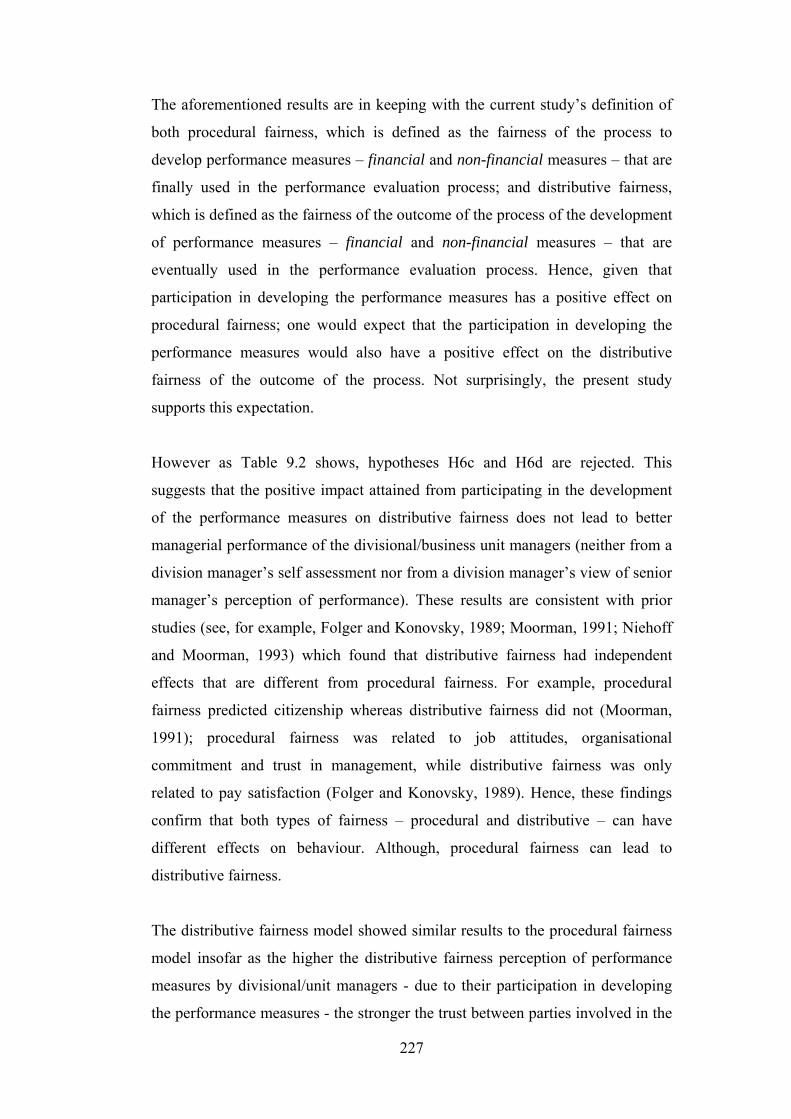
The aforementioned results are in keeping with the current study’s definition of

both procedural fairness, which is defined as the fairness of the process to

develop performance measures – financial and non-financial measures – that are

finally used in the performance evaluation process; and distributive fairness,

which is defined as the fairness of the outcome of the process of the development

of performance measures – financial and non-financial measures – that are

eventually used in the performance evaluation process. Hence, given that

participation in developing the performance measures has a positive effect on

procedural fairness; one would expect that the participation in developing the

performance measures would also have a positive effect on the distributive

fairness of the outcome of the process. Not surprisingly, the present study

supports this expectation.

However as Table 9.2 shows, hypotheses H6c and H6d are rejected. This

suggests that the positive impact attained from participating in the development

of the performance measures on distributive fairness does not lead to better

managerial performance of the divisional/business unit managers (neither from a

division manager’s self assessment nor from a division manager’s view of senior

manager’s perception of performance). These results are consistent with prior

studies (see, for example, Folger and Konovsky, 1989; Moorman, 1991; Niehoff

and Moorman, 1993) which found that distributive fairness had independent

effects that are different from procedural fairness. For example, procedural

fairness predicted citizenship whereas distributive fairness did not (Moorman,

1991); procedural fairness was related to job attitudes, organisational

commitment and trust in management, while distributive fairness was only

related to pay satisfaction (Folger and Konovsky, 1989). Hence, these findings

confirm that both types of fairness – procedural and distributive – can have

different effects on behaviour. Although, procedural fairness can lead to

distributive fairness.

The distributive fairness model showed similar results to the procedural fairness

model insofar as the higher the distributive fairness perception of performance

measures by divisional/unit managers - due to their participation in developing

the performance measures - the stronger the trust between parties involved in the

227

evaluation process. This result contradicts Folger and Konovsky’s (1989) finding

which showed that distributive fairness was not related to trust in management;

rather only procedural fairness was related to trust in management.

One possible explanation for this inconsistent result could be that the current

study’s construct of distributive fairness differed from the one employed in

Folger and Konovsky’s (1989) study, which used employees’

compensation/payment to investigate distributive fairness. Folger and Konovsky

(1989) argue that when an employees’ compensation/payment has been paid for

by the organisation they work with, there is no reason for employees to put any

further trust or commitment towards that organisation. This is why they

concluded that only procedural fairness was related to trust, while distributive

fairness was related to pay satisfaction. Unlike Folger and Konovsky (1989),

distributive fairness in this current research refers to the fairness of the outcome

of the process of the development of performance measures that were eventually

used in the performance evaluation process. Hence, when the divisional/business

unit managers perceived that the performance measures - as the outcome of the

process of development to be used in the performance evaluation process - are

fair, it is not surprising when it has a positive effect on trust between the parties

involved in the performance evaluation process. A proposition the current

research finding supports.

In line with the procedural fairness model, the distributive fairness model in this

current study also fails to support hypothesis H4. This suggests that the

participation in the development of performance measures does not directly

impact the trust between parties involved in the performance evaluation process.

However, this participation has a positive effect on trust via a higher distributive

fairness in the performance measures due to participation. This means that the

relationship between participation in developing performance measures, and the

trust between parties involved in the performance evaluation process, was

mediated by the distributive fairness of the performance measures.

Furthermore, similar to the procedural fairness model, the distributive fairness

model in the current research also fails to support hypotheses H7a and H7b. This

228

suggests that trust between parties involved in the performance evaluation

process does not have a positive impact on managerial performance of the

divisional/business unit managers. This is based on the division manager’s self-

assessment as well as from the division manager’s view of senior manager’s

perception of performance. This finding is consistent with prior research (see, for

example, Konovsky and Cropanzano, 1991; MacKenzie et al., 2001; Dirks and

Ferrin, 2002; Mayer and Gavin, 2005) which found that there is no relationship

between trust and performance as explained in Section 9.3.1.

In summary, the distributive fairness model provided strong evidence for some

of the arguments in the proposed research model. The distributive fairness model

is illustrated in Figure 9.3.

Figure 9.3: The distributive fairness model

Distributive Fairness (DFAIR)

Common- Measures Bias

(CMB)


Trust (TRST)


9.3.3 Financial vs. Non-financial Fairness From the hypotheses testing H3 was rejected. This suggests that divisional

managers perceive financial measures as being fairer in comparison to the non-

financial measures. This result is different to the results of Lau and Sholihin

(2005) who found that there were no differences between financial and non-

229

financial measures in terms of their importance in affecting job satisfaction.

Additionally, although Kaplan and Norton (1993, 2001) argue that non-financial

measures are one of the important strengths of the BSC, in the present study;

divisional managers perceived that financial measures were fairer than non-

financial measures. This might be because of the subjectivity of non-financial

measures (Ittner et al., 2003).

9.3.4 Summary of the Hypotheses Testing Findings The findings of the current research can be summarised as follows.

1. Participation (PRTCPT)

Participation in the development of performance measures positively

influences the common-measure bias as well as the fairness perception

for both procedural fairness and distributive fairness. Moreover,

participation did not have a positive effect on trust between parties

involved in the performance evaluation process.

2. Common-Measure Bias (CMB)

The positive effect of participation in the development of performance

measures reduces the common-measure bias problem, which leads to a

positive effect on managerial performance.

3. Fairness Perception (PFAIR and DFAIR)

Fairness perception of the performance measures, for both procedural

fairness and distributive fairness, positively affects the trust between

parties involved in the performance evaluation process. Additionally,

fairness perception mediates the relationship between participation and

trust. However, only procedural fairness perception has a positive

influence on managerial performance.

4. Trust (TRST)

In the present study, trust between parties involved in the performance

evaluation process does not have a positive impact on managerial

performance.

230

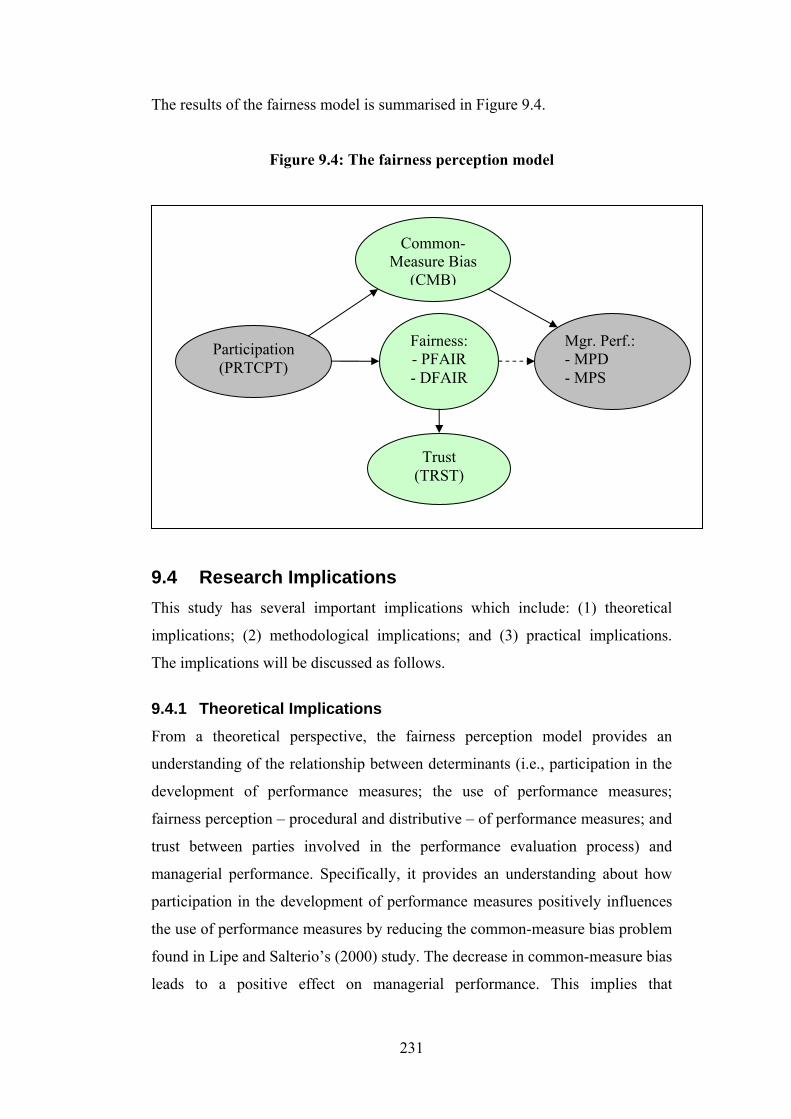
The results of the fairness model is summarised in Figure 9.4.

Figure 9.4: The fairness perception model



(CMB)


Trust (TRST)


9.4 Research Implications This study has several important implications which include: (1) theoretical

implications; (2) methodological implications; and (3) practical implications.

The implications will be discussed as follows.

9.4.1 Theoretical Implications From a theoretical perspective, the fairness perception model provides an

understanding of the relationship between determinants (i.e., participation in the

development of performance measures; the use of performance measures;

fairness perception – procedural and distributive – of performance measures; and

trust between parties involved in the performance evaluation process) and

managerial performance. Specifically, it provides an understanding about how

participation in the development of performance measures positively influences

the use of performance measures by reducing the common-measure bias problem

found in Lipe and Salterio’s (2000) study. The decrease in common-measure bias

leads to a positive effect on managerial performance. This implies that

231

participation in the development of performance measures is an effective method

to reduce the common-measure bias problem found in the BSC environment.

Furthermore, participation in the development of performance measures also

influences the fairness (i.e., procedural and distributive) perception of the

performance measures, which ultimately influences the trust between parties

involved in the performance evaluation process. This implication is in

accordance with prior research (see, for example, Thibaut and Walker, 1975;

Folger, 1977; Greenberg, 1986b, Kanfer et al., 1987; Paese et al., 1988; Lind and

Tyler, 1988; Greenberg, 1990a; Lind et al., 1990; Tyler, 1990; Tyler and Lind,

1992; Organ and Moorman, 1993; Shapiro, 1993; Korsgaard and Roberson,

1995; Muhammad, 2004) which demonstrated that participation was one of the

drivers of procedural fairness. Additionally, this current study showed that

procedural fairness can enhance distributive fairness, which is also consistent

with prior studies (see, for example, Laventhal, 1980; Folger and Greenberg,

1985; Lind and Tyler, 1988; Greenberg, 1990b; Tyler and Bies, 1990; Korsgaard

and Roberson, 1995). Furthermore, both types of fairness perception (i.e.,

procedural and distributive) were found to have similar effects on trust. This

result contradicts Folger and Konovsky’s (1989) finding which showed that only

procedural fairness is related to trust in management.

Another theoretical implication was that participation in the development of

performance measures does not directly influence the trust between parties

involved in the performance evaluation process. Rather, this participation

influences the trust via the fairness perception of either procedural fairness or

distributive fairness. Consequently, fairness perception mediates the relationship

between participation and trust.

Additionally, only procedural fairness was demonstrated to have a positive

influence on managerial performance. This finding implies that although

procedural fairness can lead to distributive fairness, both types of fairness

perception (procedural and distributive) can have different effects on behaviour.

This finding is consistent with prior studies (see, for example, Folger and

Konovsky, 1989; Moorman, 1991; Niehoff and Moorman, 1993) which found

232

that distributive fairness had independent effects that are different to procedural

fairness.

9.4.2 Methodological Implications The methodology used in this current research provides guidelines for further

research in this area of study, specifically, in the case of studying performance

measures for Australian companies. The guidelines include: the approach to

survey managers who hold very high positions; questionnaire design; data

collection procedures including survey mail-out and follow-up; and the method

used to analyse the data. These guidelines are reviewed below.

1. To reduce the response bias from a mail questionnaire survey, it is very

important to design the questionnaire carefully. Initial contact should be

made by telephone and/or e-mail to make sure that the correct address of

respondents is obtained. Furthermore, conducting a pilot test is

recommended prior to undertaking the actual survey. Additionally, to

increase the response rate, a follow-up procedure is crucial.

2. It is important to test the reliability and the validity of the data both in the

pilot testing data and in the final data.

3. Data analysis with SEM, using AMOS, to test the hypotheses proposed is

recommended for theory testing where the proposed research model has

been decided prior to the collection of the data. This is because the SEM

method has many advantages over the multi-variate method (Byrne,

2001).

4. In the case of a non-normal data distribution, the Boolen-Stine p-value

approach is recommended as a bootstrapping method.

9.4.3 Practical Implications The key findings provide significant practical implications not only for divisional

(business unit) managers within Australian public companies, but also to all of

the decision-makers that are involved in the performance evaluation process, as

well as for academics. Incorporating the findings presented in Chapters 7 and 8, a

number of practical implications can be derived. They are, the implications of

using the fairness perception model, which provides an understanding about the

relationship between participation in developing performance measures; the use

233

of performance measures (reducing common-measure bias problem); fairness

perception (procedural and distributive fairness) of the performance measures;

trust between parties involved in the performance evaluation process; and


1. Managers or decision-makers who are involved in the performance

evaluation process should consider participation in the development of

the performance measures to be used. This is important since

participation has a significant positive effect in reducing the common-

measure bias problem and increasing managerial performance.

Participation also has a significant influence on the fairness perception

(procedural and distributive) of the performance measures, which

increases the trust between parties in the performance evaluation process.

2. Managers or decision-makers should consider the importance of

procedural fairness perception of the performance measures, since it has a

positive effect on managerial performance. For instance, procedural

fairness studies (see, for example, Brownell, 1982; Dunk, 1989; Folger

and Konovsky, 1989; Moorman, 1991; Ross, 1994; Korsgaard and

Roberson, 1995; Lau et al., 1995; Lau and Tan, 1998; Lau and Lim,

2002a) have found that a procedural fairness perception of the decision-

making process will result in more positive behaviour, including better


3. Performance measures, either financial or non-financial, should be

chosen carefully in order to capture accurately the division (business unit)

strategies and its capabilities.

9.5 Limitations of the Study As with other empirical studies, the present research also has some limitations.

The limitations associated with this current study are as follows.

1. There are limitations associated with the survey questionnaire method.

Although care was taken to reduce the limitation of the method, possible

response biases may still exist.

2. The sample in this current study was selected from the top 300 companies

listed in ASX based on their equity value. Therefore, it is unclear if the

234

results are generalisable to smaller-sized companies as well as non-listed

companies. Although t-tests were performed that supported the

generalisability of the data and its results, generalising the results should

still be made with caution.

3. The current study only used divisional/business unit managers as the

respondent. Thus, data relating to questions about the agreement of the

senior managers about the divisional/business unit manager’s

performance was based on the divisional/business unit manager’s view of

the senior manager’s perception of performance. The result may have

been different had data also been obtained from the senior managers.

4. Finally, the relatively small amount of sample data reduces the power of

the statistical tests.

9.6 Suggestions for Further Research Apart from the limitations of the current study, the present research provides the

opportunity for future research, as follows.

1. Examine the fairness perception in terms of each type of the measurement

perspective in the BSC environment, ranging from the most financial

measures to the most non-financial measures (i.e., from financial,

consumer, internal business process, and learning and growth

perspectives).

2. The findings in the present research that are inconsistent with theoretical

expectations suggest that future research is still required to examine

issues in this area.

3. The findings in the present study suggested that a diversity of

performance measures is applied in each of the divisions. This provides

an opportunity to examine whether the performance measures chosen

really captures the strategy of the division and/or whether the

performance measures lead to the achievement of the organisation

objectives.

4. The use of in-depth interviews for further studies exploring the fairness

perception of performance measure issue.

235

236

5. The use of motivation and communication theories can provide the basis

for future research in examining issues in the area of trust and managerial

performance.

6. Referring to limitation number 3, the findings provide opportunity for

further study which can incorporate both divisional/business unit

managers and senior managers as the respondent.

9.7 Summary This chapter summarised the key findings in the current study, the demographic

characteristic findings as well as the hypotheses testing in accordance with the

present research’s objectives. It also provided the theoretical, methodological and

practical implications for those who are interested in investigating the effect of

fairness perception of performance measures. Finally, the limitations of the

present research were acknowledged along with the opportunity for further

research.

References Abernethy, M. A., W. F. Chua, P. F. Luckett, and F. H. Selto. 1999. Research in

managerial accounting: Learning from others’ experiences. Accounting and Finance 39 (1): 1-28.

Adams, J. S. 1965. Inequity in social exchange, in Advances in Experimental

Social Psychology, edited by L. Berkowitz, Vol. 2: 267-299. New York: Academic Press.

Adams, J. S. and S. Freedman. 1976. Equity theory revisited: Comments and

annotated bibliography, in Advances in Experimental Social Psychology, edited by L. Berkowitz, and E. Walster, Vol. 9: 43-90. New York: Academic Press.

Allison, G. T. 1971. Essence of decision: Explaining the Cuban missile issues.

Boston: Little, Brown. Amir, A., and B. Lev. 1996. Value relevance of nonfinancial information: The

wireless communications industry. Journal of Accounting and Economics 22: 3-30.

Anderson, J. C., and D. W. Gerbing. 1988. Structural equation modelling in

practice: A review and recommended two-step approach. Psychological Bulletin 103 (3): 411-423.

Andrews, F. M. 1984. Construct validity and error components of survey

measures: A structural modelling approach. Public Opinion Quarterly 48 (2): 409-442.

Aram, J. D., and P. F. Salipante, Jr. 1981. An evaluation of organisational due

process in the resolution of employee/employer conflict. Academy Management Review 6: 197-204.

Arbuckle, J. L. 2006a. AmosTM 7.0 User’s Guide. Chicago, IL, U.S.A: Amos

Development Corporation. --------. 2006b. AmosTM (Version 7.0) [Computer Program]. Chicago: SPSS. Argyris, C. 1953. Some characteristics of successful executive. The Personnel

Journal 32 (2): 50-55. --------. 1964. Integrating the individual and the organization. New York: Wiley. Arvey, R. D. 1979. Fairness in Selecting Employees. Reading MA: Addison-

Wesley. Aulakh, P. S., M. Kotabe, and A. Sahay. 1996. Trust and performance in cross-

border marketing partnerships: A behavioural approach. Journal of International Business Studies 27 (5): 1005-1032.

237

Baddeley, A. 1994. The magical number seven: still magic after all these years?

Psychological Review 101 (2): 353-356. Baird, K. M., G. L. Harrison, and R. C. Reeve, 2004. Adoption of activity

management practices: A note on the extent of adoption and the influence of organisational and cultural factors. Management Accounting Research 15 (4): 383-399.

Baier, A. 1986. Trust and antitrust. Ethics 96 (2): 231-260. Banker, R. D., G. Potter, and D. Srinivasan. 2000. An empirical investigation of

an incentive plan that includes nonfinancial performance measures. The Accounting Review 75 (1): 65-92.

Banker, R. D., H. Chang, and M. J. Pizzini. 2004. The balanced scorecard:

judgmental effects of performance measures linked to strategy. The Accounting Review 79 (1): 1-23.

Banker, R. D., and S. M. Datar. 1989. Sensitivity, precision, and linier

aggregation of signals for performance evaluation. Journal of Accounting Research 27 (1) Spring: 21-39.

Barret-Howard, E., and T. R. Tyler. 1986. Procedural justice as a criterion in

allocation decisions. Journal of Personality and Social Psychology 50 (2): 296-304.

Baron, R. M., and D. A. Kenny. 1986. The moderator-mediator variable

distinction in social psychological research: Conceptual, strategic and statistical considerations. Journal of Personality and Social Psychology 51 (6): 1173-82.

Bauner, J. S., J. J. Goodnow, and A. Austin. 1956. A Study of Thinking. New

York: Wiley. Bentler, P. M., and T. Raykov. 2000. On measures of explained variance in

nonrecursive structural equation models. Journal of Applied Psychology 85 (1): 125-131.

Berger, J., M. Zelditch, B. Anderson, and B. P. Cohen.1972. Structural aspects of

distributive justice: A status-value formulation, in Sociological Theories in Progress, edited by J. Berger, M. Zelditch, and B. Anderson, 21-45. Boston: Houghton Mifflin.

Bittlestone, R. 1994. “Just how well are we doing?” Director 47: 44-7. Blenkinsop, S. A., and N. Burns. 1992. Performance measurement revisited.

International Journal of Operations & Production Management 12 (10): 16-25.

238

Blomqvist, K. 1997. The many faces of trust. Scandinavian Journal of

Management 13 (3): 271-286. Blum, M. L., and J. C. Naylor. 1968. Industrial Psychology: Its Theoretical and

Social Foundations, New York, NY: Harper and Row. Bollen, K. A., and R. A. Stine. 1992. Bootstrapping goodness-of-fit measures in

structural equation models. Sociological Methods and Research 21 (2): 205-229.

Borman, W. C., and D. H. Brush. 1993. More progress toward a taxonomy of

managerial performance requirements. Human Performance 6 (1): 1-21. Bourne, M., J. Mills, M. Wilcox, A. Neely, and K. Platts. 2000. Designing,

implementing and updating performance measurement systems. International Journal of Operations & Production Management 20 (7): 754-771.

Bright, J., R. E. Davies, C. A. Downes, and R.C. Sweeting. 1992. The

deployment of costing techniques and practices: A UK study. Management Accounting Research 3 (3): 201-211.

Brownell, P., 1982. The role of accounting data in performance evaluation,

budgetary participation, and organisational effectiveness. Journal of Accounting Research 20 (1) Spring: 12-27.

Brownell, P., and A. S. Dunk. 1991. Task uncertainty and its interaction with

budgetary participation and budget emphasis: Some methodological issues and empirical investigation. Accounting Organisation and Society 16 (8): 693-703.

Brownell, P., and M. K. Hirst. 1986. Reliance on accounting information,

budgetary participation, and task uncertainty: Tests of a three-way interaction. Journal of Accounting Research 24 (2) (Autumn): 241-249.

Brownell, P., and M. McInnes. 1986. Budgetary participation, motivation, and

managerial performance. The Accounting Review LXI (4): 587-600. Browne, M. W. 1982. Covariance Structures, in Topics in Applied Multivariate

Analysis, edited by D.M. Hawkins. New York: Cambridge University Press.

Burgess, T. F., T. S. Ong, and N. E. Shaw. 2007. Traditional of contemporary?

The prevalence of performance measurement system types. International Journal of Productivity and Performance Management 56 (7): 583-602.

Byrman, A., and D. Cramer. 1990. Quantitative Data Analysis for Social

Scientist, London: Routledge.

239

Byrne, B. M. 2001. Structural Equation Modelling with AMOS: Basic Concepts, Applications, and Programming, Mahwah New Jersey: Lawrence Erlbaum Associates Inc.

--------. 2006. Structural Equation Modelling with EQS: Basic Concepts,

Applications, and Programming, Mahwah New Jersey: Lawrence Erlbaum Associates Inc.

Chenhall, R. H., and K. Langfield-Smith. 2003. Performance measurement and

reward systems, trust, and strategic change. Journal of Management Accounting Research 15: 117-143.

Chow, C. W., K. M. Haddad, and J. E. Williamson, 1997. Applying the balanced

scorecard to small companies. Management Accounting 79 (2): 21-27. Coakes, S. J., L. Steed, and J. Price. 2008. SPSS Version 15.0 for Windows:

Analysis Without Anguish, 1st ed. Milton, Qld: John Wiley & Sons Australia, Ltd.

Coakes, S. J., and L. Steed. 2007. SPSS Version 14.0 For Windows: Analysis

Without Anguish, Milton, Queensland: John Wiley & Sons Australia, Ltd. Cohen, J. 1988. Statistical Power Analysis for the Behavioral Sciences, 2nd ed.

Hillsdale, NJ: Lawrence Erlbaum Publishing. Cohen, R. L. 1987. Distributive justice: Theory and research. Social Justice

Research 1 (1): 19-40. Cullen, J. B., J. L. Johnson, and T. Sakano. 2000. Success through commitment

and trust: The soft side of strategic alliance management. Journal of World Business 35 (3): 223-240.

Cunningham, E. 2008. A Practical Guide to Structural Equation Modelling

Using AmosTM. Melbourne: Statsline. Cropanzano, R., and J. Greenberg. Progress in Organisational Justice: Tunneling

Through the Maze, in International Review of Industrial and Organisational Psychology, edited by Cooper, C.L., and Robertson, I.T. New York: John Willey and Sons, in press.

Crosby, F. 1976. A Model of egoistical relative deprivation. Psychological

Review 83 (2): 85-113. --------. 1984. Relative deprivation in organisational settings, in Research in

Organisational Behaviour, edited by B.M. Staw, and L.L. Cummings, 6: 51-93. Greenwich, C.T.: JAI Press.

Daniel, S. J., and W. D. Reitsperger. 1991. Linking quality strategy with

management control systems: Empirical evidence from Japanese industry. Accounting, Organizations and Society 16 (7): 601-618.

240

Daniel, S. J., W. D. Reitsperger, and T. Gregson. 1995. Quality consciousness in Japanese and US electronics manufacturers: An examination of the impact of quality strategy and management controls systems on perceptions of the importance of quality to expected management rewards. Management Accounting Research 6 (4): 367-382.

Deluga, R. J. 1995. The relation between trust in the supervisor and subordinate

organizational citizenship behaviour. Military Psychology 7 (1): 1-16. de Vaus, D. A. 1992. Surveys in Social Research, London: Allen and Unwin. Deutch, M. 1958. Trust and Suspicion. Journal of Conflict Resolution 2: 265-

279. Dilla, W. N., and P. J. Steinbart. 2005. Relative weighting of common and

unique balanced scorecard measures by knowledgeable decision makers. Behavioral Research in Accounting 17: 43-53.

Dillman, D. A. 2007. Mail and Internet Surveys: The Tailored Design Method,

2nd Edition, United States of America: John Wiley & Sons, Inc. Dirks, K. T., and D. L. Ferrin. 2002. Trust in leadership: Meta-analytic findings

and implications for research and practice. Journal of Applied Psychology 87 (4): 611-628.

Dodgson, M. 1993. Learning, trust and technological collaboration. Human

Relations 46 (1): 77-95. Drucker, P. F. 1990. The emerging theory of manufacturing. Harvard Business

Review 68 (May-June): 94-102. Drucker, P. 1974. Management: Tasks, Responsibilities, and Practice, New

York: Harper and Row. Dunk, A. S. 1989. Budget emphasis, budgetary participation and managerial

performance: A note. Accounting Organisations and Society 14 (4): 321-324.

--------. 1991. The effects of job-related tension on managerial performance in

participative budgetary settings. In Conference Proceeding of the Accounting Association of Australia and New Zealand (July): 246-249.

Durkheim, E. 1964. The division of labor in society. New York: Free Press. Earley, P. C. 1986. Trust, perceived importance of praise and criticism, and work

performance: An examination of feedback in the United States and England. Journal of Management 12 (4): 457-473.

Eccles, R. G. 1991. The performance measurement manifesto. Harvard Business

Review 69 (January-February): 131-137.

241

Fayol, H. 1916. Administration Industrielle et générale [Industrial and general administration]. Paris: Dunod.

Feltham, G. A., and J. Xie. 1994. Performance measure congruity and diversity

in multi-task principal/agent relations. The Accounting Review 69 (3): 429-453.

Folger, R. 1977. Distributive and procedural justice: Combined impact of

“voice” and improvement on experienced inequity. Journal of Personality and Social Psychology 35 (2): 108-119.

--------. 1987. Distributive and procedural justice in the workplace. Social Justice

Research 1 (2): 143-160. Folger, R., and M. A. Konovsky. 1989. Effects of procedural and distributive

justice on reactions to pay raise decisions. Academy of Management Journal 32 (1): 115-130.

Folger, R., and J. Greenberg. 1985. Procedural justice: An interpretive analysis

of personnel systems, in Research in Personnel and Human Resources Management, edited by K. Rowland, and G. Ferris, 3: 141-183. Greenwich, C.T.: JAI Press.

Foster, G., and L. Sjoblom. 1996. Quality improvement drivers in the electronics

industry. Journal of Management Accounting Research 8: 55-86. Fry, W. R., and G. Cheney. 1981. Perceptions of procedural fairness as a

functions of distributive preference. Paper presented at the meeting of the Midwestern Psychological Association, Detroit, M.I.

Fry, W. R., and G. S. Laventhal. 1979. Cross-situational procedural preferences:

A comparison of allocation preferences and equity across different settings, in. The Psychology of Procedural Justice, edited by A. Lind (Chair), symposium presented at the meeting of the American Psychological Association. Washington, D.C.

Fryxell, G. R., and M. E. Gordon.1989. Workplace justice and job satisfaction as

predictors of satisfaction with union and management. Academy of Management Journal 32 (4): 851-866.

Fryxell, G. E., R. S. Dooley, and M. Vryza. 2002. After the ink dries: The

interaction of trust and control in U.S.-based international joint ventures. Journal of Management Studies 39 (6): 865-886.

Fuller, L. 1961. The adversary system, in Talks on American Law, edited by H.

Berman, 10-22. New York: Vintage Books. Gambetta, D. 1988. Mafia: The price of distrust, in Trust – Making and Breaking

Relationships, edited by D. Gambetta, pp. 213-238. Oxford: Basil Blackwell.

242

Garson, G. D. n. d. 2008. "Path Analysis" from Statnotes: Topics in Multivariate Analysis [cited 13 May 2008]. Available from http://www2.chass.ncsu.edu/garson/pa765/statnote.htm.

Ghalayini, A. M., J. S. Noble, and T. J. Crowe. 1997. An integrated dynamic

performance measurement system for improving manufacturing competitiveness. International Journal of Production Economics 48: 207-225.

Glover, J. 1994. Profiting through trust. International Management September:

38-40. Gravetter, F., and L. Wallnau. 2000. Statistics for the Behavioural Sciences, 5th

Edition, Belmont, CA: Wadsworth. Greenberg, J., and R. L. Cohen. 1982. Why justice? Normative and instrumental

interpretations, in Equity and Justice in Social Behaviour, edited by J. Greenberg, and RL Cohen, pp. 437-469. New York: Academic Press.

Greenberg, J. 1984. On the apocryphal nature of inequity distress, in The Sense

of Injustice, edited by R. Folger, 167-188. New York: Plenum. --------. 1986a. Determinants of perceived fairness of performance evaluations.

Journal of Applied Psychology 71 (2): 340-342. --------. 1986b. The distributive justice of organisational performance

evaluations, in Justice in Social Relations, edited by H. W. Hierhoff, R. L. Cohen, and J. Greenberg, 337-351. New York: Plenum.

--------. 1987. A taxonomy of organisational justice theories. Academy of

Management Review 12 (1): 9-22. --------. 1990a. Organisational justice: Yesterday, today, and tomorrow. Journal

of Management 16 (2): 399-432. --------. 1990b. Looking fair versus being fair: Managing impressions of

organisational justice. Research in Organisational Behaviour 12: 111-157.

Greenberg, J., and G. S. Laventhal. 1976. Equity and the use of over-reward to

motive performance. Journal of Personality and Social Psychology 34 (2): 179-190.

Hair, J. F. Jr., R. E. Anderson, R. L. Tatham, and W. C. Black. 1998.

Multivariate Data Analysis, 4th Edition, Upper Saddle River, N.J.: Prentice-Hall.

Hair, J. F. Jr., W. C. Black, B. J. Babin, R. E. Anderson and R. L. Tatham. 2006.

Multivariate Data Analysis, 6th Edition, New Jersey: Prentice Hall, Pearson Education, Inc.

243

http://www2.chass.ncsu.edu/garson/pa765/statnote.htm

Hallén, L., and M. Sandström. 1991. Relationship atmosphere in international business. New Perspective on International Marketing: 108-125.

HassabElnaby, H. R., A. A. Said, and B. Wier. 2005. The retention of

nonfinancial performance measures in compensation contracts. Journal of Management Accounting Research 17: 23-42.

Hayduk, L. A. 1987. Structural Equation Modelling with LISREL: Essential and

Advances, Baltimore, Maryland: The John Hopkins University Press. Hemphill, J. K. 1959. Job descriptions for executives. Harvard Business Review

37: 55-67. Heneman, H. G. 1974. Comparison of self and superior ratings of managerial

performance. Journal of Applied Psychology 59 (5): 638-42. Heneman, R. L. 1986. The relationship between supervisory ratings and results-

oriented measures of performance: A meta-analysis. Personnel Psychology 39 (4): 811-827.

Herbig, P., and J. Milewicz. 1993. The relationship of reputation and credibility

of brand success. Journal of Consumer Marketing 10 (3): 18-24. Hibbets, A., M. R. Roberts, and T. L. Albright. 2006. Common-measures bias in

the balanced scorecard: Cognitive effort and general problem-solving ability. In MAS (Conference Paper).

Hirst, M. K. 1981. Accounting information and the evaluation of subordinate

performance: A situational approach. Accounting Review 56 (4): 771-784. --------. 1983. Reliance on accounting performance measures, task uncertainty,

and dysfunctional behaviour: Some extensions. Journal of Accounting Research 21 (2): 596-605.

Holmbeck, G. N. 1997. Toward terminological, conceptual, and statistical clarity

in the study of mediators and moderators: Examples from the child-clinical and pediatric psychology literatures. Journal of Consulting and Clinical Psychology 65 (4): 599-610.

Holmes-Smith, P., E. Cunningham, and L. Coote. 2006. Structural Equation

Modeling: From the Fundamentals to Advanced Topics. Melbourne: Statsline.

Homans, G. C. 1961. Social Behaviour: Its Elementary Forms, New York:

Harcourt, Brace, and World. Hopwood, A. G. 1972. An empirical study of the role of accounting data in

performance evaluation. Journal of Accounting Research 10. Empirical Research in Accounting: Selected Studies 1972: 156-182.

244

Horne, J. H. and T. Lupton. 1965. The work activities of middle managers: An exploratory study. Journal of Management Studies 2 (1): 14-33.

Hu, L. T., and P. M. Bentler. 1998. Fit indices in covariance structure modelling:

Sensitivity to underparameterized model misspecification. Psychological Methods 3 (4): 424-453.

Inkpen, A. C. and S. C. Currall. 1997. International joint venture trust: An

empirical examination, in Cooperative Strategies: North American Perspective, edited by P. W. Beamish, and J. P. Killing, pp. 308-334. San Francisco: New Lexington Press.

Innes, J., and F. Mitchell. 1998. A Practical Guide to Activity Based Costing,

The Chartered Institute of Management Accountants (CIMA), Kogan Page Limited, London.

Ittner, C. D., D. F. Larcker, and M. V. Rajan. 1997. The choice of performance

measures in annual bonus contracts. The Accounting Review 72 (2): 231-255.

Ittner, C. D., and D. F. Larcker. 1996. Measuring the impact of quality initiatives

on firm financial performance. Advances in the Management of Organisational Quality 1: 1-37.

-------. 1998a. Innovations in performance measurement: Trends and research

implications. Journal of Management Accounting Research 10: 205-238. -------. 1998b. Are nonfinancial measures leading indicators of financial

performance? An analysis of customer satisfaction. Journal of Accounting Research 36 (3-Supplement):1-35.

-------. 2001. Assesing empirical research in managerial accounting: A value

based management perspective. Journal of Accounting and Economics 32: 349-410.

-------. 2003. Coming up short on nonfinancial performance measurement.

Harvard Business Review 81 (11): 88-95. Ittner, C. D., D. F. Larcker, and M. Meyer. 2003. Subjectivity and the weighting

of performance measures: Evidence from a balanced scorecard. The Accounting Review 78 (3): 725-758.

Jain, D. 1994. Regression analysis for marketing decisions. In Principles of

Marketing Research, edited by R. P. Bagozzi. Cambridge, England: Blackwell Basil, 162-194.

Jasso, G. 1980. A new theory of distributive justice. American Sociological

Review 45 (1): 3-32.

245

Johnson, H. T., and R. S. Kaplan. 1987. Relevance Lost - the Rise and Fall of Management Accounting. Boston, MA: Harvard Business School Press.

Johnson, J. W., R. J. Schneider, and F. L. Oswald. 1997. Toward a taxonomy of

managerial performance profiles. Human Performance 10 (3): 227-250. Johansson, I-L., and G. Baldvinsdottir. 2003. Accounting for trust: Some

empirical evidence. Management Accounting Research 14 (3): 219-234. Jöreskog, K. G. 1969. A general approach to confirmatory maximum likelihood

factor analysis. Psychometrika 34 (2): 183-202. --------. 1993. Testing structural equation models. In B.M. Byrne (2006),

Structural Equation Modelling with EQS: Basic Concepts, Applications and Programming, 2nd Ed. Mahwah New Jersey: Lawrence Erlbaum Associates Inc.

Kalagnanam, S. S., and R. M. Lindsay. 1999. The use of organic models of

control in JIT firms: Generalizing Woodward’s findings to modern manufacturing systems. Accounting, Organizations and Society 24 (1): 1-30.

Kanfer, R., J. Sawyer, P. C. Early, and E. A. Lind. 1987. Fairness and

participation in evaluation procedures: Effects on task attitudes and performance. Social Justice Research 1 (2): 235-249.

Kaplan, S. E., and J. T. Mackey. 1992. An examination of the association

between organizational design factors and the use of accounting information for managerial performance evaluation. Journal of Management Accounting Research 4: 116-130.

Kaplan, R. S. 1983. Measuring manufacturing performance: A new challenge for

managerial accounting research. The Accounting Review LVIII (4): 686-704.

Kaplan, R. S., and A. A. Atkinson. 1998. Advanced Management Accounting, 3rd

Edition, Upper Saddle River, N. J.: Prentice Hall. Kaplan, R. S., and D. P. Norton. 1992. The balanced scorecard – measures that

drive performance. Harvard Business Review 70 (1): 71-79. -------. 1993. Putting the balanced scorecard to work. Harvard Business Review

71 (5): 134-42. -------. 1996a. Using the balanced scorecard as strategic management system.

Harvard Business Review 74 (1): 75-85. -------. 1996b. The balanced scorecard: Translating strategy into action. Boston,

MA: Harvard Business School Press.

246

-------. 2001. The strategy-focused organisation: How balanced scorecard companies thrive in the new business environment. Boston, MA: Harvard Business School Press.

Katz, R. L. 1974. Skills of an effective administrator. Harvard Business Review

52 (5): 90-102. Kenis, I. 1979. Effects of budgetary goal characteristics on managerial attitudes

and performance. Accounting Review 54 (4): 707-721. Kennedy, J. 1995. Debiasing the curse of knowledge in audit judgment. The

Accounting Review 70 (2): 249-273. Kerlinger, F. N., and H. B. Lee. 2000. Foundations of behavioral research, 4th

Edition, United States of America: Wadsworth Thomson Learning, Inc. Kerlinger, F. N. 1986. Foundations of behavioral research. New York: CBS

Publishing Japan, Ltd. Klammer, T., B. Koch, and N. Wilner. 1991. Capital budgeting practices – a

survey of corporate use. Journal of Management Accounting Research 3: 113-130.

Kline, R. B. 2005. Principle and practice of structural equation modelling.

Second Edition, New York: The Guilford Press. Konovsky, M.A., and R. Cropanzano. 1991. Perceived fairness of employee drug

testing as a predictor of employee attitudes and job performance. Journal of Applied Psychology 76 (5): 698-707.

Korsgaard, M. A., E. M.Whitener, and S. E. Brodt. 2002. Trust in the face of

conflict: The role of managerial trustworthy behaviour and organizational context. Journal of Applied Psychology 87 (2): 312-319.

Korsgaard, M. A., and L. Roberson. 1995. Procedural justice in performance

evaluation: The role of instrumental and non-instrumental voice in performance appraisal discussions. Journal of Management 21 (4): 657-669.

Kurtz, K., C. Miao, and D. Gentner. 2001. Learning by analogical bootstrapping.

Journal of the Learning Sciences 10 (4): 417-446. Laitinen, E. K. 2001. Management accounting change in small technology

companies: Towards a mathematical model of the technology firm. Management Accounting Research 12 (4): 507-541.

Lane, C. 1998. Introduction: Theories and issues in the study of trust, in Trust

Within Organizations and Between Organizations, edited by C. Lane, and R. Bachmann, pp. 1-30. Oxford, U. K.: Oxford University Press.

247

Lane, P. J., J. E. Salk, and M. A. Lyles. 2001. Absorptive capacity, learning, and performance in international joint ventures. Strategic Management Journal 22 (12): 1139-1161.

Lau, C. M., and M. Sholihin, 2005. Financial and nonfinancial performance

measures: How do they affect job satisfaction? The British Accounting Review 37: 389-413.

Lau, C. M., L. C. Low, and I. Eggleton. 1995. The impact of reliance on

accounting performance measures on job-related tension and managerial performance: Additional evidence. Accounting, Organisations and Society 20 (5): 359-381.

Lau, C. M., and J. J. Tan. 1998. The impact of budget emphasis, participation

and task difficulty on managerial performance: A cross cultural study of the financial service sector. Management Accounting Research 9 (2): 163-183.

Lau, C. M., and E. Lim. 2002a. The intervening effects of participation on the

relationship between procedural justice and managerial performance. British Accounting Review 34: 55-78.

-------. 2002b. The relationship between participation and performance: The

roles of procedural justice and evaluative styles. Working Paper. Laventhal, G. S., J. Karuza Jr., and W. R. Fry, 1980. Beyond fairness: A theory

of allocation preferences, in Justice and Social Interaction, edited by G. Mikula, 167-218. Bern, Switzerland: Hans Huber Publishers.

Laventhal, G. S. 1976a. Fairness in social relationship, in Contemporary Topics

in Social Psychology, edited by J.W. Thibaut, J.T. Spence, and R.C. Carson, 211-239. Morristown, N.J: General Learning Press.

-------. 1976b. The distribution of rewards and resources in groups and

organisations, in Advances in Experimental Social Psychology, edited by L. Berkowitz, and E. Walster, Vol. 9, 91-131. New York: Academic Press.

-------. 1980. What should be done with equity theory?: New approaches to the

study of fairness in social relationships, in Social Exchange: Advances in Theory and Research, edited by K.J. Gergen, M.S. Greenberg, and R.H. Willis, New York: Plenum Press.

Laventhal, G. S., and J. W. Michaels. 1969. Extending the equity model:

Perceptions of inputs and allocation of reward as a function of duration and quantity of performance. Journal of Personality and Social Psychology 12 (4): 303-309.

248

Lawler, E. E. III., and P. W. O’Gara. 1967. Effects of inequity produced by underpayment on work output, work quality and attitudes toward the work. Journal of Personality and Social Psychology 51 (5): 403-410.

Lerner, J., and P. E. Tetlock. 1999. Accounting for the effects of accountability.

Psychological Bulletin 125 (2): 255-275. Lerner, M. J. 1977. The justice motive: Some hypotheses as to its origins and

forms. Journal of Personality 45 (1): 1-52. --------. 1982. The justice motive in human relations and the economic model of

man: A radical analysis of facts and fictions, in Cooperation and Helping Behaviour: Theories and Research, edited by V. Darlega, and J. Grezlak, 121-145. New York: Academic Press.

Lerner, M. J., and L. A. Whitehead. 1980. Procedural justice viewed in the

context of justice motive theory, in Justice and Social Interaction, edited by G. Mikula, 219-256. New-York: Springer-Verlag.

Letza, S. R. 1996. The design and implementation of the balanced business

scorecard: An analysis of three companies in practice. Business Process Re-engineering & Management Journal 2 (3): 54-76.

Lewicki, R. J., and B. B. Bunker. 1996. Developing and maintaining trust in

work relationships, in Trust in Organizations, edited by R. M. Kramer, and T. Tyler, pp. 114-139. Thousand Oaks, C. A.: Sage Publications.

Lewis, D. J., and A. Weigert. 1985. Trust as a social reality. Social Forces 63

(4): 967-985. Libby, T., S. E. Salterio, and A. Webb. 2004. The balanced scorecard: The

effects of assurance and process accountability on managerial judgment. The Accounting Review 79 (4): 1075-1094.

Lingle, J., and W. A. Schiemann. 1996. From balanced scorecard to strategic

gauges: Is measurement worth it? Management Review 85 (3): 56-61. Lind, E. A., S. Kurtz, L. Musante, L. Walker, and J. W. Thibaut. 1980. Procedure

and outcome effects on reactions to adjudicated resolution of conflicts of interest. Journal of Personality and Social Psychology 39 (4): 643-653.

Lind, E., R. Kanfer, and P. Early. 1990. Voice, control, and procedural justice:

Instrumental and noninstrumental concerns in fairness judgment. Journal of Personality and Social Psychology 59 (5): 952-959.

Lind, E., and T. Tyler. 1988. The social psychology of procedural justice,

reviewed by P.G. Chevigny, v, 247. New York: Plenum.

249

Lind, E., and P. Early. 1991. Some thoughts on self and group interests: A parallel-processor model. Paper presented at the annual meeting of the Academy of Management, Miami.

Lindquist, T. 1995. Fairness as antecedent to participative budgeting: Examining

the effects of distributive justice, procedural justice and referent cognitions of satisfaction and performance. Journal of Management Accounting Research 7: 122-147.

Lipe, M. G., and S. E. Salterio. 2000. The balanced scorecard: Judgmental

effects of common and unique performance measures. The Accounting Review 75 (3): 283-298.

-------. 2002. A note on the judgmental effects of the balanced scorecard’s

information organisation. Accounting, Organisations and Society 27 (6): 531-540.

Little, H. T., N. R. Magner, and R. B. Welker. 2002. The fairness of formal

budgetary procedures and their enactment, relationship with managers behaviour. Group & Organisational Management June 27 (2): 209-225.

Little, R. J. A., and D. B. Rubin. 2002. Statistical Analysis with Missing Data,

2nd Edition, Hoboken, N. J.: Wiley. Lohman, C., L. Fortuin, and M. Wouters. 2004. Designing a performance

measurement system: A case study. European Journal of Operational Research 156 (2): 267-286.

Lorenz, E. H. 1988. Neither friends nor strangers: Informal networks of

subcontracting in French industry, in Trust – Making and Breaking Relationships, edited by D. Gambetta, pp. 194-210. Oxford: Basil Blackwell.

Luther, R. G., and S. Longden. 2001. Management accounting in companies

adapting to structural to structural change and volatility in transition economies: A South African study. Management Accounting Research 12 (3): 299-320.

Lyles, M. A., M. Sulaiman, J. Q. Barden, and A. R. B. A. Kechik. 1999. Factors

affecting international joint venture performance: A study of Malaysian joint venture. Journal of Asian Business 15 (2): 1-20.

MacKenzie, S. B., P. M. Podsakoff, and G.A. Rich. 2001. Transformational and

transactional leadership and salesperson performance. Journal of the Academy of Marketing Science 29 (2): 115-134.

Mahoney, T. A. 1975. Justice and equity: A recurring theme in compensation.

Personnel 52 (5): 60-66.

250

-------. 1983. Approaches to the definitions of comparable worth. Academy of Management Review 8 (1): 14-22.

Mahoney, T. A., T. H. Jerdee, and S. J. Carroll. 1965. The job(s) of management.

Industrial Relations 4 (2): 97-110. Malina, M. A., and F. H. Selto. 2001. Communicating and controlling strategy:

An empirical study of the effectiveness of the balanced scorecard. Journal of Management Accounting Research 13: 47-90.

March, J. G., and H. A. Simon. 1958. Organizations. New York: Wiley. Mardia, K. V. 1970. Measures of multivariate skewness and kurtosis with

applications. Biometrica 57 (3): 519-530. Marsh, C. 1982. The survey method, London: Goerge Allen and Unwin. Markman, A., and D. L. Medin. 1995. Similarity and alignment in choice.

Organisational Behavior and Human Decision Processes 63 (2): 117-130.

Martin, J. 1981. Relative deprivation: A theory of distributive injustice for an era

of shrinking resources, in Research in Organisational Behaviour, edited by L.L. Cummings, and B.M. Staw, Vol. 3: 53-107. Greenwich, C.T.: JAI Press.

Mayer, R. C., and M. B. Gavin. 2005. Trust in management and performance:

Who minds the shop while the employees watch the boss? Academy of Management Journal 48 (5): 874-888.

McDonald, R. P., and M. H. R. Ho. 2002. Principles and practice in reporting

structural equation analyses. Psychological Methods 7 (1): 64-82. McKenzie, F. D., and M. D., Shilling. 1998. Avoiding performance measurement

traps: Ensuring effective incentive design and implementation. Compensation and Benefits Review July-August 30 (4): 57.

Mia, L. 1989. The impact of participation in budgeting and job difficulty on

managerial performance and work motivation: A research note. Accounting Organizations and Society 14 (4): 347-357.

Miller, G. 1956. The magical number seven, plus or minus two: Some limits on

our capacity for information processing. The Psychological Review March 63: 81-97.

Miller, L. E., and K. Smith. 1983. Handling non-response issues, Journal of

Extension, On-line, 21 (5). Available at: http://www.joe.org/joe/1983september/83-5-a7.pdf.

251

http://www.joe.org/joe/1983september/83-5-a7.pdf

Mintzberg, H. 1973. The nature of managerial work. New York: Harper and Row.

-------. 1975. The manager’s job: Folklore and fact. Harvard Business Review 53:

49-61. Mintzberg, H., and J. Waters. 1982. Tracking strategy in an entrepreneurial firm.

Academy of Management Journal 25: 465-499. Moorman, R. H. 1991. The relationship between organizational justice and

organizational citizenship behaviors: Do fairness perceptions influence employee citizenship? Journal of Applied Psychology 76 (6): 845-855.

Moores, K., and S. Yuen. 2001. Management accounting systems and

organizational configuration: A life-cycle perspective. Accounting, Organizations and Society 26 (4/5): 351-389.

Morgan, R. M., and S. D. Hunt. 1994. Commitment-trust theory of relationship

marketing. Journal of Marketing 58 (July): 20-38. Morse, J. J., and F. R. Wagner. 1978. Measuring the process of managerial

effectiveness. Academy of Management Journal 21 (1): 23-35. Mossholder, K. W., N. Bennett, and C. L. Martin. 1998. A multilevel analysis of

procedural justice context. Journal of Organisational Behaviour 19 (2): 131-141.

Muhammad, A. H. 2004. Procedural justice as mediator between participation in

decision-making and organisational citizenship behaviour. International Journal of Commerce & Management 14 (3 & 4): 58-68.

Nagy, M. S. 2002. Using a single-item approach to measure facet job

satisfaction. Journal of Occupational and Organizational Psychology 75 (1): 77-86.

Nazari, J., T. Kline, and I. Herremans. 2006. Conducting survey research in

management accounting, in Methodological Issues in Accounting Research: Theories and Methods, edited by Z. Hoque, pp. 427-459. London: Spiramus Press Ltd.

Neely, A. 1999. The performance measurement revolution: Why now and what

next? International Journal of Operations & Production Management 19 (2): 205-228.

Neely, A., M. Gregory, and K. Platts. 1995. Performance measurement system design: A literature review and research agenda. International Journal of Operations & Production Management 15 (4): 80-116.

252

Newsom, J. 2005. Practical approaches to dealing with non-normal and categorical variables. http://www.ioa.pdx.edu/newsom/semclass/ho_estimate2.doc.

Niehoff, B. P., and R. H. Moorman. 1993. Justice as a mediator of the

relationship between methods of monitoring and organisational citizenship behaviour. Academy of Management Journal 36 (3): 527-556.

Nisbett, R. E., and L. Ross. 1980. Human inference. Englewood Cliffs, N. J.:

Prentice-Hall. Oakes, G. 1990. The sales process and the paradoxes of trust. Journal of

Business Ethics 9 (8): 671-679. Olsen, E. O., H. Zhou, D. M. S. Lee, Y. E. Ng, C. C. Chong, and P. Padunchwit.

2007. Performance measurement system and relationship with performance results: A case analysis of a continuous improvement approach to PMS design. International Journal of Productivity and Performance Management 56 (7): 559-582.

Olve, N. G., J. Roy, and M. Wetter. 1999. Performance drivers: A practical

guide to using the balanced scorecard, New York: John Wiley & Sons. Organ, D.W., and R. H. Moorman. 1993. Fairness and organisational citizenship

behaviour: What are the connections? Social Justice Research 6 (1): 5-18. Oshagbemi, T. 1999. Overall job satisfaction: How good are single versus

multiple-item measures? Journal of Managerial Psychology 14 (5): 388-403.

Otley, D. T. 1978. Budget use and managerial performance. Journal of

Accounting Research 16 (1) Spring: 122-149. -------. 1999. Performance management: A framework for management control

systems research. Management Accounting Research 10 (4): 363-382. -------. 2001. Extending the boundaries of management accounting research:

Developing systems for performance management. British Accounting Review 33 (3): 243-261.

Paese, P. W., E. A. Lind, and R. Kanfer. 1988. Procedural fairness and work

group responses to performance evaluation systems. Social Justice Research 2 (3): 193-205.

Pallant, J. 2005. SPSS survival manual: A step by step guide to data analysis

using SPSS, 2nd Edition, Crows Nest, NSW: Allen and Unwin. Payne, J., J. Bettman, and E. Johnson. 1993. The adaptive decision maker.

Cambrige, UK: Cambrige University Press.

253

http://www.ioa.pdx.edu/newsom/semclass/ho_estimate2.doc

Pearce, J. L. 1993. Toward an organizational behaviour of contract laborers: Their psychological involvement and effects on employee co-workers. Academy of Management Journal 36 (5): 1082-1096.

Pettit, J. D., J. R. Goris., and B.C. Vaught. 1997. An Examination of

Organizational Communication as a moderator of the relationship between job performance and job satisfaction. The Journal of Business Communication 34 (1): 81-98.

Pillai, R., C. A. Schriesheim, and E. S. Williams. 1999. Fairness perceptions and

trust as mediators for transformational and transactional leadership: A two-sample study. Journal of Management 25 (6): 897-933.

Pinsonneault, A., and K. L. Kraemer. 1993. Survey research methodology in

management information systems: An assessment. Journal of Management Information Systems 10 (2): 75-106.

Podsakoff, P. M., S. B. MacKenzie, and W. H. Bommer. 1996. Transformational

leader behaviors and substitutes for leadership as deteminants of employee satisfaction, commitment, trust, and organizational citizenship behaviors. Journal of Management 22 (2): 259-298.

Prien, E. P., and R. E. Liske. 1962. Assessments of higher-level personnel: III. A

comparative analysis of supervisor ratings and incumbent self-ratings of job performance. Personnel Psychology 15 (2): 187-194.

Principles of Human Research Ethics (http://research.vu.edu.au/ordsite/hrec.php) Pritchard, R. D., M. D. Dunnette, and D. O. Jorgenson. 1972. Effects of

perceptions of equity and inequity on worker performance and satisfaction. Journal of Applied Psychology 56 (1): 75-94.

Radhakrishna, R., and P. Doamekpor. 2008. Strategies for generalizing findings

in survey research. Journal of Extension 46 (2): 1-4. Retrieved 05/06/2008 from http://www.joe.org/joe/2008april/tt1p.shtml.

Read, W. H. 1962. Upward communication in industrial hierarchies. Human Relations 15 (1): 3-15.

Rich, G. A. 1997. The sales manager as a role model: Effects on trust, job

satisfaction, and performance of salespeople. Journal of the Academy of Marketing Science 25 (4): 319-328.

Roberts, E. S. 1999. In defence of the survey method: An illustration from a

study of user information satisfaction. Accounting and Finance 39 (1): 53-77.

Roberts, M. L., T. L. Albright, and A. R. Hibbets. 2004. Debiasing balanced

scorecard evaluations. Behavioral Research in Accounting 16: 75-88.

254

http://research.vu.edu.au/ordsite/hrec.php

http://www.joe.org/joe/2008april/tt1p.shtml

Robson, M. J., C. S. Katsikeas, and D. C. Bello. 2008. Drivers and performance outcomes of trust in international strategic alliances: The role of organizational complexity. Organization Science 19 (4): 647-665.

Ross, A. 1994. Trust as a moderator of the effect of performance evaluation style

on job related tension: A research note. Accounting, Organisations and Society 19 (7): 629-635.

Rotter, J. B. 1967. A new scale for the measurement of interpersonal trust.

Journal of Personality 35 (4): 651-665. Sabel, C. F. 1993. Studies trust: Building new forms of cooperation in a volatile

economy. Human Relations 46 (9): 1133-1170. Said, A A., H. R. HassabElnaby, and B. Wier. 2003. An empirical investigation

of the performance consequences of nonfinancial measures. Journal of Management Accounting Research 15: 193-223.

Sarkar, M. B., R. Echambadi, S. T. Cavusgil, and P. S. Aulakh. 2001. The

influence of complementarity, compatibility, and relationship capital on alliance performance. Journal of Academic Marketing Science 29 (Fall): 358-373.

Schafer, J. L. 1997. Analysis of incomplete multivariate data. London: Chapman

and Hall. Schurr, P. H., and J. L. Ozanne. 1985. Influences on exchange processes:

Buyer’s preconception of a seller’s trustworthiness and bargaining toughness. Journal of Consumer Research 11 (4): 939-953.

Schwinger, T.1980. Just allocations of goods: Decisions among three principles,

in Justice and Social Interaction, edited by G. Mikula, pp. 95-125. New York: Plenum.

Sekaran, U. 2003. Research methods for business: A skill building approach, 4th

Edition, United States of America: John Wiley and Sons, Inc. Shanteau, J. 1988. Psychological characteristics and strategies of expert decision

makers. Acta Psychologica 68 (1-3) September: 203-215. Shapiro, D. L., and J. M. Brett. 1993. Comparing three processes underlying

judgments of procedural justice: A field study of mediation and arbitration. Journal of Personality and Social Psychology 65 (6): 1167-1177.

Shapiro, D. 1993. Reconciling theoretical differences among procedural justice

research by re-evaluating what it means to have one’s views “considered”: Implications for third party managers, in Justice in the workplace: Approaching fairness in human resource management, edited by R. Cropanzano, pp. 51-78. Hillsdale, N. J.: Erlbaum.

255

Sharma, S. 1996. Applied multivariate techniques. NJ: John Wiley and Sons, Inc. Sheppard, B. H. 1984. Third-party conflict intervention: A procedural

framework, in Research in Organisational Behaviour, edited by B. M. Staw, and L. L. Cummings, Vol. 6: 141-190. Greenwich, C.T.: JAI Press.

Shields, M. D., and S. M. Young. 1993. Antecedents and consequences of

participative budgeting: Evidence of the effects of asymmetrical information. Journal of Management Accounting Research 5: 265-280.

Silk, S. 1998. Automating the balanced scorecard. Management Accounting

(May): 38-44. Sim, K. L., and L. N. Killough. 1998. The performance effects of

complementarities between manufacturing practices and management accounting systems. Journal of Management Accounting Research 10: 325-346.

Simon, H. A. 1945. Administrative behavior: A study of decision making

processes in administrative organizations. New York: Free Press. Simonson, I., and B. Staw. 1992. De-escalation strategies: A comparison of

techniques for reducing commitment to losing courses of action. Journal of Applied Psychology 77 (4): 419-427.

Singh, P. J., and A. J. R. Smith. 2001. TQM and innovation: An empirical

examination of their relationship. Paper presented to 5th International and 8th National Research Conference on Quality and Innovation Management, Victoria, Australia, retrieved 8 August 2006. http://www.eacc.unimelb.edu.au/pubs/proceedings6.pdf#search=%22TQM%20and%20Innovation%3A%20An%20Empirical%20Examination%22.

Six, F., and A. Sorge. 2008. Creating a high-trust organization: An exploration

into organization policies that stimulate interpersonal trust building. Journal of Management Studies 45 (5): 857-884.

Skinner, W. 1986. The productivity paradox. Harvard Business Review 64 (July-

August): 55-59. Slovic, P., and D. MacPhillamy, 1974. Dimensional commensurability and cue

utilisation in comparative judgment. Organisational Behavior and Human Performance 11: 172-194.

Slovic, P., and S. C. Lichtenstein. 1971. Comparison of bayesian and regression

approaches to the study of information processing in judgment. Organisational Behavior and Human Performance 6: 649-744.

Smith, P. H., E. Cunningham, and L. Coote. 2006. Structural equation modeling:

From the fundamentals to advanced topics. Melbourne: Statsline.

256

http://www.eacc.unimelb.edu.au/pubs/proceedings6.pdf#search=%22TQM%20and%20Innovation%3A%20An%20Empirical%20Examination%22



Stewart, R. 1972. Studies of managerial jobs. International Studies of Management and Organisation 2: 7-37.

--------. 1975. Management education and our knowledge of manager’s jobs.

International Studies of Management and Organisation 5: 73-89. Stryker, P. 1958. On the meaning of executive qualities. Fortune (June): 116-

119, 186, 189. Suncorp-Metway Ltd, 2006. Suncorp Annual Report, retrieved 22 March 2007.

http://www.suncorp.com.au/suncorp/personal/default.aspx?home. Swan, J. E., F. I. Trawick, and D. W. Silva. 1985. How industrial salespeople

gain customer trust. Industrial Marketing Management 14 (3): 203-211. Tetlock, P. 1985. Accountability: The neglected social context of judgment and

choice. Research in Organisational Behavior 7: 297-332. Thibaut, J., and L. Walker. 1975. Procedural justice: A psychological analysis.

Hilsdale, NJ: Erlbaum. --------. 1978. A theory of procedure. California Law Review 66: 541-566. Tomkins, C. 2001. Interdependencies, trust and information in relationships,

alliances and networks. Accounting, Organisations and Society 26 (2): 161-191.

Tornblom, K. Y. 1990. In press. The social psychology of distributive justice, in

KThe Nature and Administration of Justice: Interdisciplinary Approaches, edited by Scherer. Cambridge, England: Cambridge University Press.

Tornow, W. W., and P. R. Pinto. 1976. The development of a managerial job

taxonomy: A system for describing, classifying, and evaluating executive positions. Journal of Applied Psychology 61 (4): 410-418.

Thornton, G. C. 1968. The relationship between supervisory and self-appraisals

of executive performance. Personnel Psychology, 41: 441-456. Tyler, T. R. 1990. Why people obey the law. New Haven, CT: Yale University

Press. --------. 1994. Psychological models of the justice motive: Antecedents of

distributive and procedural justice. Journal of Personality and Social Psychology 67 (5): 850-863.

Tyler, T. R., and R. J. Bies. 1990. Beyond formal procedures: The interpersonal

context of procedural justice, in Advances in Applied Social Psychology: Business Settings, edited by J. Carrol, pp. 77-98., Hillsdale, NJ: Lawrence Erlbaum.

257

http://www.suncorp.com.au/suncorp/personal/default.aspx?home

Tyler, T., and E. Lind. 1992. A relational model of authority in groups, in Advances in Experimental Social Psychology, edited by M. Zanna, 25: 115-192. New York: Academic Press.

Van Avermaet, E., C. McClintoch, and J. Moskowitz. 1978. Alternative

approaches to equity: Dissonance reduction, pro-social motivation and strategies accommodation. European Journal of Social Psychology 8 (4): 419-437.

Van der Stede, W. A., S. M. Young, and C. X. Chen. 2005. Assessing the quality

of evidence in empirical management accounting research: The case of survey studies. Accounting, Organisations and Society 30 (7-8): 655-684.

Veal, A. J. 2005. Business research methods: A managerial approach. NSW:

Pearson Australia Group Pty Ltd. Wagner, S. L., and M. C. Rush. 2000. Altruistic organizational citizenship

behaviour: Context, Disposition, and Age. The Journal of Social Psychology 140 (3): 379-391.

Walker, L., E. A. Lind, and J. Thibaut. 1979. The relation between procedural

justice and distributive justice. Virginia Law Review 65: 1401-1420. Walster, E., E. Berscheid, and G. W. Walster. 1973. New directions in equity

research. Journal of Personality and Social Psychology 25 (2):151-176. Walton, R. W., and R. B. McKersie. 1965. A behavioural theory of labour

negotiations. New York: McGraw-Hill. Wanous, J. P., A. E. Reichers, and M. J. Hudy. 1997. Overall job satisfaction:

How good are single-item measures? Journal of Applied Psychology 82 (2): 247-252.

West, S. G., J. F. Finch, and P. J. Curran. 1995. Structural equation models with

nonnormal variables: Problems and remedies, in Structural Equation Modelling: Concepts, Issues, and Applications, edited by R.H. Hoyle, pp. 56-75. Thousand Oaks, CA: Sage.

Widener, S. K., and F. H. Selto. 1999. Management control systems and

boundaries of the firm: Why do firms outsource internal auditing activities? Journal of Management Accounting Research 11: 45-73.

Wothke, W. 1993. Nonpositive definite matrices in structural modelling, in

Testing Structural Equation Models, edited by K. A. Bollen, and J. S. Long, pp. 256-293. Newbury Park, CA: Sage.

Yim, A. T. 2001. Renegotiation and relative performance evaluation: Why an

informative signal may be useless. Review of Accounting Studies 6: 77-108.

258

Young, S. M. 1996. Survey research in management accounting: A critical assessment, in Research Methods in Accounting: Issues and Debates, edited by, A. J. Richardson. CGA Canada Research Foundation.

Young, L. C., and I. F. Wilkinson. 1989. The role of trust and co-operation in

marketing channels: A preliminary study. European Journal of Marketing 23 (2): 109-122.

Yung, Y.-F., and P. M. Bentler. 1996. Bootstrapping techniques in analysis of

mean and covariance structures, in Advanced Structural Equation Modelling: Issues and Techniques, edited by G. A. Marcoulides and R. E. Schumacker, pp. 195-226. Mahwah, NJ: Lawrence Erlbaum Associates.

Zhang, S., and A. B. Markman. 2001. Processing product unique features:

Alignability and involvement in preference construction. Journal of Consumer Psychology 11 (1): 13-27.

Zhu, W. 1997. Making bootstrap statistical inferences: A tutorial. Research

Quarterly for Exercise and Sport 68 (1): 44-55.

259

260

APPENDIX I

PART A

QUESTIONNAIRE SURVEY

QUESTIONNAIRE SURVEY A Covering Letter

School of Accounting and Finance Faculty of Business and Law

Footscray Park Campus Ballarat Road, Footscray

Victoria University, Melbourne Victoria 8001, Australia

Date: ------------- Dear Divisional Manager, I am conducting a survey of divisional/unit managers of the top 300 largest companies listed on the Australian Stock Exchange (ASX), as measured by market value of equity as of June 30, 2006 as part of my PhD program. The aim of this research project is to promote a greater understanding of the role of participation in enhancing the fairness perception of measurement, and interpersonal trust between parties in the performance evaluation process. The project has approval of the University Human Research Ethics Committee. The selection of divisional/unit managers to be asked to participate in this study was chosen from information contained in the Annual Report of the top 300 largest companies. Your response will greatly appreciated, and assist in ensuring the research results are representative and meaningful. I hope this research will be of interest to you, and to the wide academic and professional community. At your earliest convenience could you place the completed questionnaire in the reply paid envelope, and return it to me, preferably by 7 December, 2007. I assure you that all responses will be confidential. The data will be summarized and only the summarized data, with no identifying features, will be reported in the report and any subsequent publications. Should you have any queries about this research please contact my principal supervisor Dr. Albie Brooks, or myself on the details of which are below. Thank you very much for your participation. Yours Sincerely, Anni Aryani Dr. Albie Brooks PhD Candidate Senior Lecturer School of Accounting and Finance School of Accounting and Finance Victoria University – Australia Victoria University – Australia Phone: +613-9919 1451 Phone: +613-9919 4631 Email: [email protected] Email: [email protected]

261

mailto:[email protected]


SURVEY

Effects of Participation on Fairness Perception of Performance Measures

Overview This survey investigates the role of participation in enhancing the fairness perception of performance measures, and interpersonal trust between parties in the performance evaluation process. This is the first national study of its kind that aims to bring insight to organizations relating to performance measures and the performance evaluation process.

Definitions Performance Measures: All performance measures (financial and non-financial) that

are commonly used in the performance evaluation process to evaluate divisional (unit) manager performance.

Procedural Fairness: The fairness of the process to develop performance measures –

financial and non-financial measures – that are finally used in the performance evaluation process.

Distributive Fairness: The fairness of the outcome of the process of the development of

performance measures – financial and non-financial measures – that are used in the performance evaluation process (i.e. the actual measures).

Instructions for Completing this Survey

1. Please answer all the survey questions to the best of your ability. 2. We welcome any additional comments in the space provided at the end of the

survey. 3. Please place the completed survey in the enclosed reply-paid envelope and return it

at your earliest convenience. Thank you for supporting this research project

262

Part 1: Participation in Performance Measures Development The following statements relate to managers’ participation in the determination of financial and non-financial (e.g. customer satisfaction, administrative expense/total revenue (%), employee satisfaction) measures of performance; and the weighting of each measure of performance. Please circle a number for each statement to indicate the extent of your agreement.

No

Bas

is

For

Ans

wer

ing

Stro

ngly

D

isag

ree

Dis

agre

e

Neu

tral

Agr

ee

Stro

ngly

Ag

ree

1. I am allowed a high degree of influence in the determination of financial measures used to measure performance of my division (unit).

0 1 2 3 4 5

2. I am allowed a high degree of influence in the determination of non-financial measures used to measure performance of my division (unit).

0 1 2 3 4 5

3. I am allowed a high degree of influence in the determination of the weighting of the performance measures for which I am accountable in my division (unit).

0 1 2 3 4 5

4. I really have little voice in the formulation of the performance measures of my division (unit)

0 1 2 3 4 5

5. The setting of the performance measures of my division (unit) is pretty much under my control.

0 1 2 3 4 5

6. My senior manager asks for my opinions and thoughts when determining my division (unit) performance measures.

0 1 2 3 4 5

7. My division (unit) performance measures are not finalized until I am satisfied with it.

0 1 2 3 4 5

8. The division’s (unit) performance measures that are finally used in the performance evaluation process are based on the division’s (unit) manager input.

0 1 2 3 4 5

9. I am allowed a high degree of influence in the determination of the target of each of the financial measure used to measure performance of my division (unit).

0 1 2 3 4 5

10. I am allowed a high degree of influence in the determination of the target of each of the non-financial measure used to measure performance of my division (unit).

0 1 2 3 4 5

263

Part 2: Fairness of Performance Measures The following propositions relate to the perceived fairness of the development of the performance measures. Please circle a number for each statement to indicate the extent of your agreement. Part 2.1: Procedural Fairness

No

Bas

is

For

Ans

wer

ing

Stro

ngly

D

isag

ree

Dis

agre

e

Neu

tral

Agr

ee

Stro

ngly

Ag

ree

1. The procedure for preparing the financial measures to evaluate divisional (unit) performance is applied consistently among the divisions (units).

0 1 2 3 4 5

2. All units are treated similarly by respectively considering the non-financial measures of each division (unit).

0 1 2 3 4 5

3. The procedures for preparing the financial measures include provisions for an appeal process.

0 1 2 3 4 5

4. The procedures for preparing the non-financial measures include provisions for an appeal process.

0 1 2 3 4 5

5. The procedure for determining divisional (unit) financial performance measures provides sufficient opportunity for divisions (units) managers to present views and opinions before the performance measures are finalized.

0 1 2 3 4 5

6. The procedure for determining divisional (unit) non-financial performance measures provides sufficient opportunity for divisions (units) managers to present views and opinions before the performance measures are finalized.

0 1 2 3 4 5

7. The divisional (unit) performance measures are based on accurate information and informed opinion.

0 1 2 3 4 5

8. The division (unit) performance measures are determined by the senior manager in an unbiased manner.

0 1 2 3 4 5

264

Part 2.2: Distributive Fairness

No

Bas

is

For

Ans

wer

ing

Stro

ngly

D

isag

ree

Dis

agre

e

Neu

tral

Agr

ee

Stro

ngly

Ag

ree

1. The performance measures that have been used in the performance evaluation process are fair.

0 1 2 3 4 5

2. The performance measures that have been used in the performance evaluation process fairly measure my past year’s performance.

0 1 2 3 4 5

Part 2.3: Fairness of Financial vs Non-Financial

No

Bas

is

For

Ans

wer

ing

Stro

ngly

D

isag

ree

Dis

agre

e

Neu

tral

Agr

ee

Stro

ngly

Ag

ree

1. In my opinion the non-financial measures are fairer than the financial measures in the performance evaluation process of each division (unit).

0 1 2 3 4 5

2. In my opinion the non-financial measures are more realistic than the financial measures to evaluate each division (unit)’s performance.

0 1 2 3 4 5

Part 3: Interpersonal trust measures The following questions relate to interpersonal trust between parties in the performance evaluation process. Please circle a number for each statement to indicate the extent of your agreement.

No

Bas

is

For

Ans

wer

ing

Stro

ngly

D

isag

ree

Dis

agre

e

Neu

tral

Agre

e

Stro

ngly

Ag

ree

1. My senior manager takes advantage of opportunities that come up to further my interest by his/her actions and decisions.

0 1 2 3 4 5

2. I feel free to discuss with my senior manager the problems and difficulties I have in my job without jeopardizing my position or having it ‘held against’ me later on.

0 1 2 3 4 5

3. I feel confident that my senior manager keeps me fully and frankly informed about things that might concern me.

0 1 2 3 4 5

4. Senior managers at times must make decisions which seem to be against the interests of their division/unit managers.

0 1 2 3 4 5

5. When this happened to me as a division/unit manager, I believe that my senior manager’s decision is justified by other considerations.

0 1 2 3 4 5

265

Part 4: Managerial Performance Your Perception The following is a list of eight functions of managerial performance and overall effectiveness of the functions. Please rate your performance as division (unit) manager in the following functions by circling the number indicating the perception of your performance.

No

Bas

is

For

Ans

wer

ing

Ext

rem

ely

Poor

B

elow

Av

erag

e A

vera

ge

Abo

ve

Aver

age

Exce

llent

1. Planning (i.e. determining goals, policies, and courses of action) function in my division (unit) is

0 1 2 3 4 5

2. Investigating (i.e. collecting and preparing information, usually in the form of records, reports and accounts) function in my division (unit) is

0 1 2 3 4 5

3. Coordinating (i.e. exchanging information with people in the organization other than subordinates in order to relate and adjust programs) function in my division (unit) is

0 1 2 3 4 5

4. Evaluating (i.e. assessment and appraisal of proposals or of reported or observed performance) function in my division (unit) is

0 1 2 3 4 5

5. Supervising (i.e. directing, leading and developing subordinates) function in my division (unit) is

0 1 2 3 4 5

6. Staffing (i.e. maintaining the work force of a unit or of several units) function in my division (unit) is

0 1 2 3 4 5

7. Negotiating (i.e. purchasing, selling, or contracting for goods or services) function in my division (unit) is

0 1 2 3 4 5

8. Representing (i.e. advancing general organizational interests through speeches, consultation, and contacts with individuals or groups outside the organization) function in my division (unit) is

0 1 2 3 4 5

9. Overall, my performance in my division (unit) is

0 1 2 3 4 5

266

Part 5: (1) Use of Performance Measures. The following statements have been made about the use of performance measures in divisional (unit) performance evaluation. Please circle a number for each statement to indicate the extent of your agreement.

No

Bas

is

For

Ans

wer

ing

Stro

ngly

D

isag

ree

Dis

agre

e

Neu

tral

Agr

ee

Stro

ngly

Ag

ree

1. My senior manager uses all of the performance measures (financial and non-financial) to evaluate my individual performance.

0 1 2 3 4 5

2. My senior manager uses all of the performance measures (financial and non-financial) to evaluate my performance when comparing it with other divisional/unit managers.

0 1 2 3 4 5

3. My senior manager uses all of the performance measures (financial and non-financial) to evaluate my performance as divisional (unit) manager as well as the divisional (unit) performance.

0 1 2 3 4 5

4. My senior manager places more weight on financial measures to evaluate my performance.

0 1 2 3 4 5

5. My senior manager places more weight on non-financial measures to evaluate my performance.

0 1 2 3 4 5

Part 5: (2) General Perceptions Relating to Performance Measures. Please circle a number for each statement to indicate the extent of your agreement.

No

Bas

is

For

Ans

wer

ing

Stro

ngly

D

isag

ree

Dis

agre

e

Neu

tral

Agre

e

Stro

ngly

Ag

ree

1. My performance as a divisional (unit) manager and the performance of the division are one and the same thing.

0 1 2 3 4 5

2. My motivation is affected by the performance measures chosen to assess my performance.

0 1 2 3 4 5

3. The uses of performance measures I perceive as being inappropriate negatively affect my performance.

0 1 2 3 4 5

4. The uses of performance measures I perceive as being appropriate positively affect my performance.

0 1 2 3 4 5

5. I try my best to reach the targets set by the performance measures.

0 1 2 3 4 5

267

Part 6: Financial and Non-financial Measures The following are lists of financial and non-financial (i.e. customer; internal process; and learning and growth) measures commonly used to evaluate managerial and divisional (business unit) performance. Please indicate the extent of your company use of each performance measures across the four perspectives to evaluate managerial and divisional (business unit) performance by circling a number. No

Performance measures

No

Bas

is

For

Ans

wer

ing

Not

at a

ll

Ver

y Li

ttle

Littl

e

Som

ewha

t

To a

gre

at

exte

nt

1. Financial Measures Perspective

a. Net profit ($) 0 1 2 3 4 5

b. Revenues/total assets (%) 0 1 2 3 4 5

c. Return on investment (%) 0 1 2 3 4 5

d. Total expenses ($) 0 1 2 3 4 5

e. Sales growth 0 1 2 3 4 5

f. Other, please specify:

g. ……………………………………………………….. 0 1 2 3 4 5

h. ……………………………………………………….. 0 1 2 3 4 5

i. ……………………………………………………….. 0 1 2 3 4 5

j. ……………………………………………………….. 0 1 2 3 4 5

k. ……………………………………………………….. 0 1 2 3 4 5

2. Customer Measures Perspective

a. Number of customers complaints (No.) 0 1 2 3 4 5

b. Market share (%) 0 1 2 3 4 5

c. Annual sales/customer ($) 0 1 2 3 4 5

d. Customer satisfaction: survey ratings (%) 0 1 2 3 4 5

e. Customer response time 0 1 2 3 4 5


g. ……………………………………………………….. 0 1 2 3 4 5

h. ……………………………………………………….. 0 1 2 3 4 5

i. ……………………………………………………….. 0 1 2 3 4 5

j. ……………………………………………………….. 0 1 2 3 4 5

k. ……………………………………………………….. 0 1 2 3 4 5

268

No

Performance measures

No

Bas

is

For

Ans

wer

ing

Not

at a

ll

Ver

y Li

ttle

Littl

e

Som

ewha

t

To a

gre

at

exte

nt

3. Internal Business Process Perspective

a. Administrative expense/total revenue (%) 0 1 2 3 4 5

b. Length of time from order delivery 0 1 2 3 4 5

c. Inventory turnover ratio (%) 0 1 2 3 4 5

d. Rate of production capacity or resources used 0 1 2 3 4 5

e. Labour efficiency variance 0 1 2 3 4 5


g. ……………………………………………………….. 0 1 2 3 4 5

h. ……………………………………………………….. 0 1 2 3 4 5

i. ……………………………………………………….. 0 1 2 3 4 5

j. ……………………………………………………….. 0 1 2 3 4 5

k. ……………………………………………………….. 0 1 2 3 4 5

4. Learning and Growth Perspective

a. R&D expense/total expense (%) 0 1 2 3 4 5

b. Cost reduction resulting from quality product improvement

0 1 2 3 4 5

c. Investment in new product support and training ($) 0 1 2 3 4 5

d. Satisfied-employee index (No.) 0 1 2 3 4 5

e. Training expenses/total expense (%) 0 1 2 3 4 5


g. ……………………………………………………….. 0 1 2 3 4 5

h. ……………………………………………………….. 0 1 2 3 4 5

i. ……………………………………………………….. 0 1 2 3 4 5

j. ……………………………………………………….. 0 1 2 3 4 5

k. ……………………………………………………….. 0 1 2 3 4 5

269

Part 7: Your Senior Manager’s Perception The following is the statement about your senior managers’ rating of your managerial performance. Please rate your agreement to the statement by circling the number indicates which best your performance.

No

Bas

is

For

Ans

wer

ing

Ext

rem

ely

Poor

B

elow

Av

erag

e A

vera

ge

Abo

ve

Aver

age

Exce

llent

1. In my most recent performance evaluation my senior manager rated my managerial performance as:

0 1 2 3 4 5

The following are the statements of your agreement of your senior managers’ rating above. Please circle a number for each statement to indicate the extent of your agreement.

No

Bas

is

For

Ans

wer

ing

Stro

ngly

D

isag

ree

Dis

agre

e

Neu

tral

Agre

e

Stro

ngly

Ag

ree

1. I agree with the way my senior manager rated my managerial performance

0 1 2 3 4 5

2. I agree with my final rating

0 1 2 3 4 5

Part 8: General Questions (Demography) Please tick in the appropriate answer. 1. Gender?

□ Male □ Female

2. Which of the following groups represents you?

□ Less than 30 years □ 30-40 years □ 41-50 years □ 51-60 years □ More than 60 years

3. In which industry is your company involved?

□ Agricultural/mining/construction □ Banking/Finance/Insurance □ Consulting/professional service □ Education/research □ Government □ Health care □ Hospitality/travel/tourism □ Manufacturing □ Media/entertainment/publishing □ Real Estate □ Retail/wholesale/distribution □ Telecommunications □ Transportation/logistics □ Others (Please specify) ………

270

4. a) At what main activity is your division/unit involved?

□ Agricultural/mining/construction □ Banking/Finance/Insurance □ Consulting/professional service □ Education/research □ Government □ Health care □ Hospitality/travel/tourism □ Manufacturing □ Media/entertainment/publishing □ Real Estate □ Retail/wholesale/distribution □ Telecommunications □ Transportation/logistics □ Others (Please specify) ………

b) What proportion of your division’s output is transferred internally?

□ 0% □ 1 – 25% □ 26 – 50% □ 51 – 75% □ > 75%

5. How long have you held your current position in this company?


6. How long have you worked for this company?


7. How many employees are you responsible for?

□ Less than 100 employees □ 100-200 employees □ 200-500 employees □ More than 500 employees

8. Would you be agreed to be interviewed as part of a follow-up study? □ Yes □ No 9. If yes, please fill in the form below or just attach your business card.

Name: Postal Address: Email: Telephone:

10. Would you like to receive a copy of the summary report of the study?

□ Yes □ No Address: …………………………………………………….. ………………………………………………………. ………………………………………………………. ………………………………………………………. ……………………………………………………….

271

Thank you very much for taking the time to complete this questionnaire. Your help in providing this information is greatly appreciated. If there is anything else you would like to tell us about, please do so in the space provided below. …………………………………………………………………………………………………………………………………………………………………………………………………………………………………………………………………………………………………………………………………………………………………………………………………………………………………………………………………………………………………………………………………………………………………………………………………………………………………………………………………………………………………………………………………………………………………………………………………………………………………………………………………………………………………………………………………………………………………………………………………………………………………………………………………………………………………………………………………………………………………………………………………………………………………………………………………………………………………………………………………………………………………………………………………………………………………………………………………………………………………………………………………………………… ………………………………………………………………………………………………………………………………………………………………………………………………………………………………………………………………………………………………………………………………………………………………………………………………………………………………………………………………………………………………………………………………………………………………………………………………………………………………………………………………………………………………………………………………………………………………………… …………………………………………………………………………………………………………………………………………………………………………………………………………………………………………………………………………………………………………………………………………………………………………………………………………………………………………………………………………………………………………………………………………………………………………………………………………………………………………………………………………………………………………………………………………………………………………

Thank you for your cooperation in completing this questionnaire. Anni Aryani Dr. Albie Brooks PhD Candidate Senior Lecturer School of Accounting and Finance School of Accounting and Finance Victoria University – Australia Victoria University – Australia Phone: +613-9919 1451 Phone: +613-9919 4631 Email: [email protected] Email: [email protected]

272



273

--- This page is blank intentionally! ---

Feedback Questionnaire Evaluation Form Please comment on each of the following: 1 Length of questionnaire

2 Readability / difficulty of questions

3 Were there any questions you would omit?

4 Are there questions you would suggest should be included?

5 Any additional comments?

274

APPENDIX I

PART B

A CODING SHEET

275

A CODING SHEET (All in numeric except specifically defined)

Code Quest.

No. Description Values Measure

Number Case number 1-1500 Scale Prtcp1 P1.1 Allowed a high degree of influence in determining

financial measures 5-point Scale

Prtcp2 P1.2 Allowed a high degree of influence in determining non-financial measures

5-point Scale

Prtcp3 P1.3 Allowed a high degree of influence in determining weighting of performance measures

5-point Scale

Prtcp4 P1.4 Have little voice in the formulation of the performance measure

5-point Scale

Prtcp5 P1.5 The setting of the performance measures of my division is pretty much under my control

5-point Scale

Prtcp6 P1.6 My senior manager asks for my opinions and thoughts 5-point Scale Prtcp7 P1.7 My division performance measures are not finalise

until I am satisfied 5-point Scale

Prtcp8 P1.8 The final division performance measures are based on the division’s manager input

5-point Scale

Prtcp9 P1.9 Allowed a high degree of influence in determining the target of each of financial measures used

5-point Scale

Prtcp10 P1.10 Allowed a high degree of influence in determining the target of each of non-financial measures used

5-point Scale

pf1 P2.1.1 The procedure for preparing the financial measures is applied consistently among divisions

5-point Scale

pf2 P2.1.2 All units are treated similarly by respectively considering non-financial measures of each division

5-point Scale

pf3 P2.1.3 The procedure for preparing the financial measures include provisions for an appeal process

5-point Scale

pf4 P2.1.4 The procedure for preparing the non-financial measures include provisions for an appeal process

5-point Scale

pf5 P2.1.5 The procedure to determining division financial performance measures provides opportunity to present views and opinions

5-point Scale

pf6 P2.1.6 The procedure to determining division non-financial performance measures provides opportunity to present views and opinions

5-point Scale

pf7 P2.1.7 The division performance measures are based on accurate information and informed opinion

5-point Scale

pf8 P2.1.8 The division performance measures are determined by the senior manager in an unbiased manner

5-point Scale

df1 P2.2.1 The performance measures are fair 5-point Scale df2 P2.2.2 The performance measures fairly measure my past

year’s performance 5-point Scale

FFvsNF1 P2.3.1 In my opinion non-financial measures are fairer than financial measures

5-point Scale

FFvsNF2 P2.3.2 In my opinion non-financial measures are more realistic than financial measures to evaluate each division

5-point Scale

Trust1 P3.1 My senior manager takes advantage of opportunities that come up to further my interest by his/her actions and decisions.

5-point Scale

Trust2 P3.2 I feel free to discuss with my senior manager the problems and difficulties I have in my job without jeopardizing my position or having it ‘held against’ me later on.

5-point Scale

276

Trust3 P3.3 I feel confident that my senior manager keeps me fully and frankly informed about things that might concern me.

5-point Scale

Trust4 P3.4 Senior managers at times must make decisions which seem to be against the interests of their division/unit managers.

5-point Scale

Trust5 P3.5 When this happened to me as a division/unit manager, I believe that my senior manager’s decision is justified by other considerations.

5-point Scale

mpd1 P4.1 Planning 5-point Scale mpd2 P4.2 Investigating 5-point Scale mpd3 P4.3 Coordinating 5-point Scale mpd4 P4.4 Evaluating 5-point Scale mpd5 P4.5 Supervising 5-point Scale mpd6 P4.6 Staffing 5-point Scale mpd7 P4.7 Negotiating 5-point Scale mpd8 P4.8 Representing 5-point Scale mpd9 P4.9 Overall 5-point Scale upm1 P5.1.1 Senior manager uses financial and non-financial

measures to evaluate individual performance 5-point Scale

upm2 P5.1.2 Senior manager uses financial and non-financial measures in comparing among division managers

5-point Scale

upm3 P5.1.3 Senior manager uses financial and non-financial measures to evaluate manager as well as division

5-point Scale

upm4 P5.1.4 Senior manager places more weight on financial measures to evaluate performance

5-point Scale

upm5 P5.1.5 Senior manager places more weight on non-financial measures to evaluate performance

5-point Scale

GenPercpPM1 P5.2.1 Performance of divisional manager is the same of division

5-point Scale

GenPercpPM2 P5.2.2 Motivation is affected by performance measures 5-point Scale GenPercpPM3 P5.2.3 Performance measures perceived inappropriate

negatively affect performance 5-point Scale

GenPercpPM4 P5.2.4 Performance measures perceived appropriate positively affect performance

5-point Scale

GenPercpPM5 P5.2.5 I try my best to reach the targets set by the performance measures

5-point Scale

FMa P6.1.a Net profit ($) 5-point Scale FMb P6.1.b Revenues/total assets (%) 5-point Scale FMc P6.1.c Return on investment (%) 5-point Scale FMd P6.1.d Total expenses ($) 5-point Scale FMe P6.1.e Sales growth 5-point Scale FMf P6.1.f Other, please specify: (string) CMa P6.2.a Number of customers complaints (No.) 5-point Scale CMb P6.2.b Market share (%) 5-point Scale CMc P6.2.c Annual sales/customer ($) 5-point Scale CMd P6.2.d Customer satisfaction: survey ratings (%) 5-point Scale CMe P6.2.e Customer response time 5-point Scale CMf P6.2.f Other, please specify: (string) IBPa P6.3.a Administrative expense/total revenue (%) 5-point Scale IBPb P6.3.b Length of time from order delivery 5-point Scale IBPc P6.3.c Inventory turnover ratio (%) 5-point Scale IBPd P6.3.d Rate of production capacity or resource used 5-point Scale IBPe P6.3.e Labour efficiency variance 5-point Scale IBPf P6.3.f Other, please specify: (string) LandGa P6.4.a R&D expense/total expense (%) 5-point Scale LandGb P6.4.b Cost reduction resulting from quality product

improvement 5-point Scale

277

278

LandGc P6.4.c Investment in new product support and training ($) 5-point Scale LandGd P6.4.d Satisfied-employee index (No.) 5-point Scale LandGe P6.4.e Training expenses/total expense (%) 5-point Scale LandGf P6.4.f Other, please specify: (string) mps1 P7.1.1 In my most recent performance evaluation my senior

manager rated my managerial performance as: 5-point Scale

mps2 P7.2.1 I agree with the way my senior manager rated my managerial performance

5-point Scale

mps3 P7.2.2 I agree with my final rating 5-point Scale Gender P8.1 Gender 2

options Nominal

Age P8.2 Age 5 opts Nominal Company P8.3 Company industry 13 opts Nominal Divisi P8.4a Divisi main activity 13 opts Nominal Output P8.4b Proportion of division’s output transferred internally 5 opts Nominal Tenure-mgr P8.5 Period held current position in the company 5 opts Nominal Tenure-com P8.6 Period worked for this company 5 opts Nominal Employees P8.7 How many employees are you responsible for? 4 opts Nominal Interviewed P8.8 Agreed to be interviewed as follow-up study 2 opts Nominal Address P8.9 If agreed to be interviewed, provide address Summary P8.10 Would you like to receive a copy of summary report

of the study? 2 opts Nominal

APPENDIX I

PART C

DESCRIPTIVE STATISTICS

279

Descriptive Statistics

N Minimum Maximum Mean Std.

Deviation Skewness Kurtosis

Statistic Statistic Statistic Statistic Statistic Statistic Std. Error Statistic

Std. Error

Prtcp1 164 .00 5.00 3.4451 1.12011 -.789 .190 .120 .377Prtcp2 164 1.00 5.00 3.8171 .87400 -.639 .190 .157 .377Prtcp3 164 1.00 5.00 3.4451 1.01675 -.487 .190 -.500 .377Prtcp4 164 1.00 5.00 1.7866 .89144 1.065 .190 .704 .377Prtcp5 164 1.00 5.00 3.1238 .98560 -.311 .190 -.821 .377Prtcp6 164 1.00 5.00 3.6768 .89261 -.992 .190 .925 .377Prtcp7 164 1.00 5.00 3.5244 .94934 -.746 .190 .116 .377Prtcp8 164 1.00 5.00 3.5366 .86080 -.874 .190 .357 .377Prtcp9 164 .00 5.00 3.4451 .94806 -1.087 .190 1.292 .377Prtcp10 164 1.00 5.00 3.6829 .84908 -.862 .190 .932 .377PF1 164 .00 5.00 3.7124 .94468 -1.647 .190 3.917 .377PF2 164 .00 5.00 3.5122 1.04199 -1.087 .190 1.349 .377PF3 164 .00 5.00 2.8171 1.19434 -.362 .190 -.546 .377PF4 164 .00 5.00 2.9085 1.18691 -.334 .190 -.649 .377PF5 164 .00 5.00 3.5244 1.05929 -1.021 .190 .946 .377PF6 164 1.00 5.00 3.6829 .85627 -.881 .190 .890 .377PF7 164 1.00 5.00 3.8171 .76147 -.944 .190 1.407 .377PF8 164 .00 5.00 3.6220 .95468 -1.275 .190 1.902 .377DF1 164 1.00 5.00 3.7317 .78402 -1.265 .190 2.175 .377DF2 164 .00 5.00 3.5915 .89178 -1.777 .190 3.375 .377FFvsNF1 164 .00 5.00 2.9146 .90264 -.489 .190 1.090 .377FFvsNF2 164 .00 5.00 2.7439 .91760 -.047 .190 .745 .377Trust1 164 .00 5.00 3.3354 1.03484 -.879 .190 .848 .377Trust2 164 1.00 5.00 3.8354 .93518 -.622 .190 -.178 .377Trust3 164 1.00 5.00 3.5793 1.00297 -.885 .190 .263 .377Trust4 164 1.00 5.00 3.6280 .75255 -.926 .190 .768 .377Trust5 164 .00 5.00 3.3049 1.12079 -1.552 .190 2.436 .377MPD1 164 2.00 5.00 3.6890 .67896 -.595 .190 .436 .377MPD2 164 2.00 5.00 3.6585 .73006 -.518 .190 .140 .377MPD3 164 2.00 5.00 3.6768 .74254 -.308 .190 -.070 .377MPD4 164 1.00 5.00 3.6646 .71167 -.547 .190 .830 .377MPD5 164 1.00 5.00 3.7256 .71209 -.474 .190 .867 .377MPD6 164 2.00 5.00 3.6098 .68742 -.116 .190 -.139 .377MPD7 164 .00 5.00 3.6037 .92424 -.969 .190 2.722 .377MPD8 164 .00 5.00 3.4146 .96505 -.916 .190 1.511 .377MPD9 164 2.00 5.00 3.5427 .63970 -.660 .190 -.043 .377UPM1 164 1.00 5.00 3.4817 .94948 -.578 .190 -.008 .377UPM2 164 .00 5.00 3.1829 1.31651 -.931 .190 .354 .377UPM3 164 .00 5.00 3.5671 1.00996 -1.289 .190 2.194 .377UPM4 164 .00 5.00 3.5732 1.05703 -.652 .190 .063 .377UPM5 164 .00 5.00 2.6402 .91937 -.037 .190 -.218 .377MPS1 164 .00 5.00 3.7622 1.16104 -2.167 .190 4.953 .377MPS2 164 .00 5.00 3.4634 1.23044 -1.525 .190 2.077 .377MPS3 164 .00 5.00 3.5305 1.21051 -1.700 .190 2.740 .377Valid N (listwise) 164

280

281

APPENDIX I

PART D

MISSING DATA ANALYSIS

MISSING DATA ANALYSIS

UNIVARIATE STATISTICS

N Mean Std. Deviation

Missing No. of Extremes(a,b)

Count Percent Low High Part1.1 164 3.2988 1.28311 0 .0 0 0Part1.2 164 3.9085 .90543 0 .0 0 0Part1.3 164 3.4207 1.11864 0 .0 0 0Part1.4 164 1.9756 1.03290 0 .0 0 0Part1.5 163 3.0736 1.03374 1 .6 0 0Part1.6 164 3.6098 1.03623 0 .0 9 0Part1.7 164 3.3902 1.11053 0 .0 0 0Part1.8 164 3.5549 .92181 0 .0 6 0Part1.9 164 3.4085 1.06139 0 .0 8 0Part1.10 164 3.6220 1.04077 0 .0 8 0Part2.1.1 163 3.8712 .98850 1 .6 . .Part2.1.2 164 3.4756 1.16414 0 .0 12 0Part2.1.3 164 2.6524 1.24139 0 .0 0 0Part2.1.4 164 2.7805 1.25834 0 .0 0 0Part2.1.5 164 3.5305 1.14272 0 .0 10 0Part2.1.6 164 3.7622 .97113 0 .0 4 0Part2.1.7 164 3.8659 .80279 0 .0 . .Part2.1.8 164 3.5793 1.02715 0 .0 9 0Part2.2.1 164 3.7500 .82429 0 .0 . .Part2.2.2 164 3.6220 .98005 0 .0 . .Part2.3.1 164 2.7317 .87989 0 .0 3 4Part2.3.2 164 2.5976 .93808 0 .0 3 5Part3.1 164 3.3171 1.08394 0 .0 11 0Part3.2 164 3.8841 1.02364 0 .0 0 0Part3.3 164 3.4695 1.08206 0 .0 10 0Part3.4 164 3.6280 .81516 0 .0 2 0Part3.5 164 3.2744 1.19983 0 .0 15 0Part4.1.1 164 3.6646 .71167 0 .0 0 0Part4.1.2 164 3.6463 .76539 0 .0 0 0Part4.1.3 164 3.6707 .76029 0 .0 0 0Part4.1.4 164 3.6707 .76029 0 .0 2 0Part4.1.5 164 3.6585 .74668 0 .0 2 0Part4.1.6 164 3.6463 .69832 0 .0 0 0Part4.1.7 164 3.5122 1.13228 0 .0 7 0Part4.1.8 164 3.3780 1.04665 0 .0 6 0Part4.1.9 164 3.7439 .64229 0 .0 1 0Part5.1.1 164 3.6646 1.06407 0 .0 7 0Part5.1.2 164 3.0976 1.36215 0 .0 0 0Part5.1.3 164 3.6037 1.09443 0 .0 10 0Part5.1.4 164 3.5610 1.11979 0 .0 6 0Part5.1.5 164 2.4695 .86814 0 .0 0 2Part5.2.1 164 3.1524 1.19094 0 .0 0 0Part5.2.2 164 3.1402 1.13444 0 .0 0 0Part5.2.3 164 2.7500 1.13708 0 .0 0 0

282

283

Part5.2.4 164 3.7988 .85930 0 .0 0 0Part5.2.5 164 4.2744 .66762 0 .0 4 0Part7.1.1 164 3.7317 1.28749 0 .0 . .Part7.2.1 164 3.4573 1.36274 0 .0 19 0Part7.2.2 164 3.4817 1.32680 0 .0 19 0

a Number of cases outside the range (Q1 - 1.5*IQR, Q3 + 1.5*IQR). b . indicates that the inter-quartile range (IQR) is zero.

EM Missing Data Analysis

Part1

.1 Part1

.2 Part1

.3 Part1

.4 Part1

.5 Part1

.6 Part1

.7 Part1

.8 Part1

.9 Part1.10

Part2.1.1

Part2.1.2

Part2.1.3

Part2.1.4

Part2.1.5

Part2.1.6

Part2.1.7

Part2.1.8

Part2.2.1

Part2.2.2

Part2.3.1

Part2.3.2

Part3.1

P

Part1.1 1

Part1.2 .536 1

Part1.3 .698 .608 1

Part1.4 -.494 -.717 -.660 1

Part1.5 .371 .402 .461 -.539 1

Part1.6 .208 .491 .275 -.565 .326 1

Part1.7 .421 .383 .494 -.537 .529 .496 1

Part1.8 .455 .488 .552 -.701 .526 .427 .680 1

Part1.9 .761 .543 .702 -.539 .509 .296 .369 .507 1

Part1.10 .430 .777 .643 -.773 .563 .539 .489 .668 .613 1

Part2.1.1 .245 .275 .140 -.087 .088 .168 .031 -.028 .321 .067 1

Part2.1.2 .311 .181 .208 -.154 .188 .318 .273 .096 .264 .099 .423 1

Part2.1.3 .308 .108 .172 -.107 .245 -.063 .019 .180 .420 .111 .302 .242 1

Part2.1.4 .254 .208 .262 -.283 .273 -.005 .057 .285 .334 .288 .267 .088 .815 1

Part2.1.5 .690 .427 .544 -.514 .483 .311 .440 .493 .716 .453 .356 .326 .295 .265 1

Part2.1.6 .343 .554 .460 -.624 .517 .578 .547 .546 .440 .621 .270 .198 .018 .183 .689 1

284

Part2.1.7 .426 .498 .500 -.522 .377 .497 .451 .507 .432 .592 .265 .312 .187 .226 .493 .557 1

Part2.1.8 .357 .447 .422 -.357 .389 .346 .242 .255 .412 .436 .390 .302 .197 .203 .395 .428 .511 1

Part2.2.1 .355 .619 .494 -.569 .533 .359 .429 .515 .447 .633 .414 .310 .196 .290 .474 .600 .617 .650 1

Part2.2.2 .447 .500 .420 -.397 .494 .361 .277 .274 .509 .418 .414 .438 .285 .256 .421 .498 .403 .652 .604 1

Part2.3.1 -.075 .085 -.103 .114 -.055 .073 -.143 -.095 .006 .002 .018 .233 .032 -.009 -.163 -.089 -.234 -.044 -.042 .081 1

Part2.3.2 -.057 -.094 -.060 .066 .119 .115 .028 .061 .012 -.037 -.002 .221 .121 .039 .040 .069 -.113 .027 -.012 .174 .641 1

Part3.1 .161 .530 .228 -.388 .130 .411 .182 .314 .233 .466 .241 .259 .005 .020 .294 .393 .486 .385 .515 .339 .000 -.043 1

Part3.2 .279 .551 .455 -.554 .289 .489 .294 .355 .298 .534 .271 .330 -.008 .099 .410 .484 .541 .408 .613 .372 -.028 -.106 .570

Part3.3 .389 .520 .540 -.588 .437 .515 .546 .500 .409 .583 .242 .396 .040 .099 .517 .551 .546 .444 .662 .423 -.009 .072 .594 .

Part3.4 .001 -.080 -.056 .091 -.016 .016 -.089 -.018 -.064 -.116 -.096 -.142 .023 -.092 -.037 -.043 .223 -.034 .053 .007 -.131 -.053 .051 .

Part3.5 .126 .170 .183 -.188 .113 .274 .016 .155 .128 .118 .177 .187 .003 .032 .206 .262 .102 .259 .306 .282 .152 .115 .112 .

Part4.1.1 .238 .219 .194 -.195 .144 .088 .182 .220 .239 .225 .106 .090 .166 .274 .280 .212 .361 .200 .222 .081 -.105 -.066 .067 .

Part4.1.2 .271 .201 .247 -.166 .326 -.020 .264 .210 .292 .185 .079 .128 .199 .244 .146 .150 .172 .044 .238 .262 -.087 .057 .047 .

Part4.1.3 .441 .402 .460 -.323 .265 .241 .349 .367 .312 .400 -.015 .074 .073 .155 .294 .234 .410 .309 .289 .194 -.124 -.118 .269 .

Part4.1.4 .183 .179 .279 -.307 .288 .272 .306 .376 .206 .369 -.015 -.009 -.076 .039 .209 .251 .269 .230 .299 .137 -.124 -.118 .150 .

Part4.1.5 .299 .208 .254 -.329 .249 .144 .287 .250 .239 .330 -.038 .096 .143 .194 .257 .124 .373 .243 .279 .074 -.187 -.224 .233 .

Part4.1.6 .119 .036 .090 -.140 .182 .105 .187 .135 .146 .161 .091 .004 -.015 -.019 .229 .174 .145 .039 .048 .001 -.175 -.041 .190 -.

Part4.1.7 .304 .399 .299 -.351 .176 .192 .201 .302 .187 .275 .044 .084 .058 .239 .315 .284 .279 .107 .263 .115 -.046 -.024 .197 .

Part4.1.8 .231 .179 .141 -.054 .016 .182 .131 .144 .153 .115 .055 .083 .073 .073 .144 .119 .192 .200 .096 .152 .064 .075 .197 -.

Part4.1.9 .280 .287 .279 -.231 .334 .190 .236 .221 .343 .258 .162 .106 .149 .203 .211 .148 .135 .273 .168 .196 .182 .093 .153 .

285

286

Part5.1.1 .177 .369 .253 -.303 .191 .509 .361 .310 .220 .311 .334 .382 .074 .096 .329 .498 .557 .302 .484 .378 .087 .030 .609 .

Part5.1.2 .145 .311 .202 -.190 .118 .340 .250 .157 .189 .217 .372 .485 .107 .048 .187 .250 .399 .323 .366 .294 .176 .165 .606 .

Part5.1.3 .159 .366 .237 -.318 .178 .452 .320 .304 .167 .331 .164 .313 .042 .048 .218 .367 .519 .266 .393 .283 .055 .017 .727 .

Part5.1.4 .169 -.088 -.028 .054 .033 -.080 -.133 -.232 .080 -.112 .083 -.041 .141 .153 .226 .044 .118 .180 .033 .049 -.263 -.269 -.173 -.

Part5.1.5 -.110 -.054 -.141 .163 .064 .028 .216 -.036 -.243 -.088 -.017 .166 -.030 -.113 -.166 -.005 .038 -.004 .036 .080 .126 .181 -.029 -.

Part5.2.1 .159 .218 .205 -.271 .338 .044 .150 .163 .149 .200 .027 .049 .140 .276 .188 .265 .028 .273 .252 .307 .033 .094 .100 .

Part5.2.2 -.046 -.035 -.018 .129 .007 -.157 -.131 -.004 -.007 -.100 .038 -.102 .179 .155 -.124 -.053 -.269 .025 .031 .142 .235 .232 -.066 -.

Part5.2.3 -.045 -.314 -.105 .434 -.140 -.151 -.151 -.259 -.093 -.417 .122 .081 .073 -.060 -.110 -.221 -.239 -.117 -.322 -.025 .098 .216 -.294 -.

Part5.2.4 .122 .031 .050 -.089 -.030 .111 .006 .095 .192 .065 .086 -.069 .124 .175 .147 .156 -.208 -.097 -.089 .171 .050 .059 .029 -.

Part5.2.5 .133 .326 .083 -.284 .176 .280 -.087 .090 .135 .371 .062 .084 -.069 .036 .130 .300 .218 .151 .192 .272 -.010 -.048 .252 .

Part7.1.1 .138 .263 .164 -.254 .187 .248 .254 .183 .153 .263 .285 .155 -.040 .005 .110 .258 .321 .183 .277 .250 -.107 -.054 .532 .

Part7.2.1 .142 .327 .183 -.249 .227 .297 .254 .187 .226 .287 .280 .253 .026 -.038 .194 .287 .370 .252 .326 .360 .067 .044 .611 .

Part7.2.2 .203 .323 .181 -.291 .233 .263 .267 .272 .286 .288 .255 .204 .106 .012 .231 .304 .361 .190 .318 .292 .064 .083 .554 .

a Little's MCAR test: Chi-Square = 83.086, DF = 96, Sig. = .823

APPENDIX II

PART A

STANDARDISED RESIDUAL COVARIANCE AND IMPLIED CORRELATIONS FOR INVESTIGATING DISCRIMINANT

VALIDITY FOR PFAIR – MPD MODEL

287

Table 1: Standarised Residual Covariance before deleting any items (indicators) for Measurement model PFAIR-MPD Standardized Residual Covariances (Group number 1 - Default model)

mpd9 mpd8 mpd7 trust5 pf8 pf7 upm3 Prtcp10 Prtcp8 mpd1 mpd2 mpd3 mpd4 m pd9 . 00 00 mpd8 -0.175 0.000 mpd7 0.014 0.573 0.000 trust5 -1.279 -1.235 0.123 0.000 pf8 -0.485 0.638 -0.745 1.183 0.000 pf7 -0.763 0.098 0.431 -1.440 0.763 0.000 upm3 -0.760 1.226 0.003 -1.334 0.085 1.087 0.000 prtcp10 -0.166 -0.734 0.442 -1.377 -0.126 0.249 -0.123 0.000 prtcp8 -0.400 -0.962 0.157 0.387 -0.697 0.955 -0.544 -0.161 0.000 mpd1 0.049 0.043 0.339 -0.200 0.036 1.312 -1.253 -1.195 -0.535 0.000 mpd2 0.816 0.372 0.997 -1.440 -1.645 -0.333 -0.615 0.532 -0.566 0.171 0.000 mpd3 0.557 -1.005 -0.667 -0.868 -0.256 1.850 -0.228 0.914 0.054 0.234 0.574 0.000 mpd4 -0.942 -0.928 -0.429 1.258 0.570 1.312 0.745 2.183 1.192 -0.105 0.302 0.788 0.000 mpd5 -0.444 0.801 0.321 -1.241 0.320 1.158 0.602 0.143 -1.119 -0.015 -1.964 0.155 -1.077 mpd6 0.366 1.423 -0.786 -2.102 -0.464 0.739 0.601 -0.462 -0.592 -0.109 -1.221 -0.549 0.485 trust1 0.676 1.333 0.806 -1.081 1.131 0.409 3.897 0.855 -0.347 -0.579 -0.694 0.957 -0.289 trust2 -1.039 -2.191 -0.757 1.031 0.349 0.634 -0.824 -0.471 -0.028 -1.063 0.000 0.490 0.847 trust3 -0.967 0.301 -0.190 -0.064 0.357 -0.389 -0.645 -0.170 -0.422 -0.896 -0.266 1.015 0.612 pf1 1.002 -0.696 -1.138 0.667 1.604 -0.198 -0.321 -2.791 -1.287 0.118 0.429 -1.244 -1.165 pf3 -0.628 1.316 0.586 0.811 1.544 -0.238 -1.175 -0.549 -0.242 1.199 0.882 -0.332 -1.176 pf5 -0.121 -0.307 0.648 0.632 -0.877 -0.505 -1.889 -0.985 -0.048 -0.339 -0.562 -0.264 0.562 pf6 -0.205 -0.494 0.196 0.599 -0.294 -0.357 -0.508 0.328 0.257 -1.179 -0.340 -0.629 1.087 upm1 -1.523 -0.081 -1.124 -0.518 1.006 2.360 0.024 -0.822 0.507 0.313 -1.739 -0.490 -0.827 upm2 0.331 1.723 2.190 0.073 2.143 1.078 0.118 -0.40 -0.873 0.409 0.352 0.778 0.623 prtcp1 -0.478 -0.289 0.613 0.317 0.360 0.298 -1.027 -0.753 -0.456 -0.643 0.512 0.954 0.422 prtcp2 0.830 0.387 0.898 -1.461 -0.513 1.049 1.072 1.338 -0.190 0.119 -0.010 0.814 0.584 prtcp4_R -0.984 -0.751 0.944 0.108 -0.777 -0.877 0.209 0.359 -0.070 -0.552 -1.186 0.013 1.482 prtcp5 0.824 -1.615 -0.741 -0.428 0.775 0.274 -0.295 -0.545 0.928 -0.961 1.807 0.412 0.803 prtcp6 -0.585 0.040 -0.390 0.426 0.391 0.657 2.032 0.126 -0.138 -0.492 -1.015 -0.499 0.941 prtcp7 -0.276 -1.558 -0.949 -0.931 -1.218 -0.101 -0.230 -0.389 0.364 -1.691 -0.104 0.141 0.890

288

Table 1: Standarised Residual Covariance before deleting any items (indicators) for Measurement model PFAIR-MPD (Continued) Standardized Residual Covariances (Group number 1 - Default model)

mpd5 mpd6 trust1 trust2 trust3 pf1 pf3 pf5 pf6 upm1 upm2 prtcp1 prtcp2 m pd9 m pd8 m pd7 tr ust5 pf8 pf7 u pm3 prt cp10 p rtcp8 mpd1 m pd2 m pd3 m pd4 m pd5 . 00 00 mpd6 1.072 0.000 trust1 0.628 1.290 0.000 trust2 -0.749 -0.432 -0.521 0.000 trust3 1.062 0.550 -0.312 0.248 0.000 pf1 -2.352 0.988 0.297 1.124 0.219 0.000 pf3 0.887 -0.640 -0.497 -2.307 -0.472 1.574 0.000 pf5 0.103 1.101 -1.239 -0.332 -0.103 1.343 1.910 0.000 pf6 -1.356 -0.589 -0.454 0.172 0.025 -0.494 -1.574 0.426 0.000 upm1 -0.334 0.720 2.500 -0.031 0.412 1.423 -1.263 -0.767 0.072 0.000 upm2 0.660 0.048 2.954 -2.151 -0.763 1.438 1.995 -0.675 -0.701 -0.261 0.000 prtcp1 1.184 -0.432 -1.357 0.056 0.090 0.725 2.266 3.720 -0.658 -1.180 -0.922 0.000 prtcp2 0.289 0.028 0.830 -0.177 -0.602 -0.254 -0.893 -0.420 -0.319 -0.189 -0.307 0.496 0.000 prtcp4_R 1.036 -0.572 0.034 0.081 0.826 -3.256 0.045 -0.180 0.191 -0.279 -0.758 0.397 -0.201 prtcp5 0.019 -0.359 -1.377 0.132 0.563 -0.531 0.478 0.583 0.986 -0.243 -0.326 -0.595 -0.694 prtcp6 -0.322 0.211 0.546 0.981 0.087 -1.319 -2.736 -1.091 1.289 2.709 0.598 -1.249 0.079 prtcp7 0.430 -0.354 -1.825 -0.673 0.924 -1.751 -1.206 0.160 0.645 0.789 -0.207 0.051 -0.801

289

290

Table 1: Standarised Residual Covariance before deleting any items (indicators) for Measurement model PFAIR-MPD (Continued) Standardized Residual Covariances (Group number 1 - Default model)

prtcp4_R prtcp5 prtcp6 prtcp7 mpd9 mpd8 mpd7 trust5 pf8 pf7 upm3 prtcp10 prtcp8 mpd1 mpd2 mpd3 mpd4 mpd5 mpd6 trust1 trust2 trust3 pf1 pf3 pf5 pf6 upm1 upm2 prtcp1 prtcp2 prtcp4_R 0.000 prtcp5 -0.428 0.000 prtcp6 0.134 -0.735 0.000 prtcp7 0.075 0.819 1.012 0.000

Table 2: Modification Indices (MIs) of Regression Weights before deleting

any Indicators for measurement model of PFAIR-MPD

Regression Weights: (Group number 1 - Default model)

M.I. Par Change mpd8 <--- trust2 4.885 -.159 mpd7 <--- upm2 4.494 .095 trust5 <--- mpd6 5.125 -.279 pf8 <--- pf1 4.156 .138 pf8 <--- upm2 6.964 .129 pf7 <--- MPD 4.152 .319 pf7 <--- CMB 5.786 .145 pf7 <--- trust5 4.773 -.091 pf7 <--- upm3 4.028 .093 pf7 <--- mpd1 5.767 .166 pf7 <--- mpd3 6.329 .159 pf7 <--- upm1 8.609 .145 upm3 <--- trust1 10.244 .172 prtcp10 <--- pf1 7.137 -.136 prtcp10 <--- prtcp2 5.412 .128 mpd2 <--- mpd5 5.286 -.169 mpd2 <--- prtcp5 4.511 .113 mpd4 <--- trust5 4.504 .093 mpd4 <--- prtcp10 6.298 .146 mpd5 <--- mpd2 7.366 -.172 mpd5 <--- pf1 5.280 -.112 trust1 <--- CMB 21.761 .398 trust1 <--- mpd8 4.227 .142 trust1 <--- upm3 29.847 .360 trust1 <--- upm1 8.604 .206 trust1 <--- upm2 20.307 .228 trust1 <--- prtcp7 6.217 -.175 trust2 <--- mpd8 12.571 -.185 trust2 <--- pf3 8.084 -.120 trust2 <--- upm2 10.420 -.124 trust3 <--- prtcp7 6.510 .135 pf1 <--- prtcp10 8.827 -.243 pf1 <--- mpd5 6.488 -.248 pf1 <--- prtcp4_R 12.001 -.269 pf3 <--- trust2 5.715 -.236 pf3 <--- upm2 4.087 .141 pf3 <--- prtcp1 4.600 .176 pf3 <--- prtcp6 8.121 -.293 pf5 <--- CMB 5.175 -.183

291

292

Table 2: Modification Indices (MIs) of Regression Weights before deleting any Indicators for measurement model of PFAIR-MPD (continued)


M.I.Par

Changepf5 <--- upm3 6.901 -0.163pf5 <--- pf1 4.789 0.145pf5 <--- pf3 9.215 0.159pf5 <--- prtcp1 27.554 0.294pf5 <--- prtcp6 4.166 -0.143pf6 <--- mpd5 4.892 -0.154pf6 <--- pf3 6.949 -0.109pf6 <--- prtcp1 4.775 -0.097pf6 <--- prtcp6 4.085 0.112upm1 <--- mpd7 4.063 -0.121upm1 <--- pf7 4.73 0.159upm1 <--- prtcp6 4.93 0.138upm2 <--- mpd7 9.362 0.277upm2 <--- pf8 5.211 0.2upm2 <--- trust2 5.507 -0.211upm2 <--- pf3 11.359 0.236prtcp1 <--- pf1 4.575 0.163prtcp1 <--- pf3 10.55 0.196prtcp1 <--- pf5 24.752 0.339prtcp2 <--- prtcp10 4.92 0.134prtcp4_R <--- pf1 11.734 -0.183prtcp5 <--- mpd2 6.42 0.216prtcp6 <--- CMB 7.201 0.199prtcp6 <--- upm3 6.887 0.15prtcp6 <--- pf3 10.114 -0.154prtcp6 <--- upm1 11.16 0.203prtcp7 <--- trust1 6.349 -0.13

Table 3: Standarised Residual Covariance after deleting nine items (indicators) for Measurement model PFAIR-MPD Standardized Residual Covariances (Group number 1 – Default model)

mpd1 mpd2 mpd3 mpd5 mpd7 mpd9 trust2 trust3 trust5 pf5 pf6 pf7m p . 0d1 0 00 mpd2 0.064 0.000 mpd3 0.047 0.361 0.000 mpd5 0.114 -1.938 0.179 0.000 mpd7 0.329 0.922 -0.798 0.487 0.000 mpd9 -0.091 0.668 0.303 -0.444 -0.091 0.000 trust2 -0.946 0.050 0.564 -0.558 -0.625 -1.001 0.000 trust3 -0.787 -0.224 1.075 1.258 -0.062 -0.938 -0.030 0.000 trust5 -0.177 -1.435 -0.863 -1.189 0.153 -1.279 0.879 -0.248 0.000 pf5 -0.161 -0.474 -0.128 0.358 0.844 -0.043 -0.147 0.062 0.663 0.000 pf6 -1.178 -0.375 -0.696 -1.262 0.219 -0.256 0.019 -0.177 0.497 0.611 0.000 pf7 1.345 -0.343 1.824 1.277 0.483 -0.787 0.552 -0.510 -1.508 -0.270 -0.507 0.000pf8 0.161 -1.587 -0.167 0.506 -0.610 -0.435 0.470 0.459 1.197 -0.462 -0.184 0.925upm1 0.661 -1.540 -0.168 0.073 -0.776 -1.329 -0.168 0.227 -0.606 -1.046 -0.454 1.900upm3 -0.433 -0.081 0.645 1.477 0.832 -0.219 -0.153 0.050 -1.117 -1.614 -0.435 1.195Prtcp2 0.187 -0.004 0.811 0.462 0.991 0.818 -0.096 -0.550 -1.468 -0.207 -0.439 0.996Prtcp4_R -0.499 -1.192 -0.009 1.203 1.024 -1.008 0.141 0.855 0.091 0.016 0.037 -0.954Prtcp5 -1.026 1.723 0.264 0.057 -0.781 0.721 0.019 0.407 -0.504 0.584 0.658 0.034Prtcp7 -1.636 -0.107 0.123 0.599 -0.868 -0.298 -0.609 0.959 -0.946 0.365 0.494 -0.175Prtcp8 -0.549 -0.617 -0.043 -1.024 0.169 -0.471 -0.067 -0.498 0.334 0.043 -0.002 0.774Prtcp10 -1.202 0.483 0.821 0.251 0.462 -0.234 -0.499 -0.237 -1.427 -0.883 0.073 0.078

293

Table 3: Standarised Residual Covariance after deleting nine items (indicators) for Measurement model PFAIR-MPD (Continued) Standardized Residual Covariances (Group number 1 - Default model)

pf8 upm1 upm3 Prtcp2 Prtcp4_R Prtcp5 Prtcp7 Prtcp8 Prtcp10

0. 00 0 0.760 0.000 0.292 0.000 0.000

-0.371 -0.334 1.420 0.000 -0.651 -0.444 0.553 -0.078 0.000 0.749 -0.482 -0.093 -0.787 -0.553 0.000

-1.089 0.624 0.116 -0.672 0.180 0.695 0.000 -0.654 0.287 -0.270 -0.188 -0.098 0.687 0.341 0.000 -0.073 -1.037 0.168 1.354 0.343 -0.768 -0.398 -0.300 0.000

294

Table 4: Implied (for all variables) Correlations for Measurement model PFAIR - MPD Implied (for all variables) Correlations (Group number 1 - Default model)

MPD TRST PFAIR CMB PRTCPT mpd1 mpd2 mpd3 mpd5 mpd7 mpd9 trust5 trust3 M P 1D T RST . 8 10 34 PFAIR 0.436 0.718 1 CMB 0.350 0.562 0.458 1 PRTCPT 0.544 0.675 0.823 0.376 1 mpd1 0.662 0.230 0.288 0.232 0.36 1 mpd2 0.452 0.157 0.197 0.158 0.246 0.299 1 mpd3 0.757 0.264 0.330 0.265 0.412 0.501 0.342 1 mpd5 0.599 0.209 0.261 0.210 0.326 0.397 0.271 0.454 1 mpd7 0.634 0.221 0.277 0.222 0.345 0.420 0.287 0.481 0.380 1 mpd9 0.474 0.165 0.207 0.166 0.258 0.314 0.214 0.359 0.284 0.301 1 trust5 0.101 0.289 0.208 0.163 0.195 0.067 0.046 0.076 0.060 0.064 0.048 1 trust3 0.307 0.881 0.632 0.495 0.595 0.203 0.139 0.232 0.184 0.195 0.145 0.255 1 trust2 0.280 0.803 0.576 0.451 0.542 0.185 0.126 0.212 0.168 0.177 0.133 0.232 0.707 pf5 0.300 0.493 0.688 0.315 0.566 0.198 0.136 0.227 0.180 0.190 0.142 0.143 0.435 pf6 0.332 0.546 0.760 0.348 0.626 0.219 0.150 0.251 0.199 0.210 0.157 0.158 0.481 pf7 0.298 0.491 0.684 0.313 0.563 0.197 0.135 0.226 0.179 0.189 0.141 0.142 0.432 pf8 0.234 0.385 0.537 0.246 0.442 0.155 0.106 0.177 0.140 0.149 0.111 0.112 0.340 upm3 0.267 0.429 0.349 0.764 0.287 0.177 0.121 0.203 0.160 0.170 0.127 0.124 0.378 upm1 0.288 0.463 0.377 0.823 0.309 0.191 0.130 0.218 0.173 0.183 0.137 0.134 0.408 Prtcp2 0.378 0.469 0.572 0.261 0.695 0.250 0.171 0.287 0.227 0.240 0.179 0.136 0.413 Prtcp4_R 0.396 0.491 0.599 0.274 0.728 0.262 0.179 0.300 0.238 0.251 0.188 0.142 0.433 Prtcp5 0.351 0.435 0.530 0.242 0.644 0.232 0.159 0.266 0.210 0.223 0.166 0.126 0.383 Prtcp7 0.398 0.493 0.602 0.275 0.731 0.263 0.180 0.301 0.239 0.252 0.189 0.143 0.435 Prtcp8 0.390 0.484 0.590 0.269 0.717 0.258 0.176 0.296 0.234 0.248 0.185 0.140 0.426 Prtcp10 0.402 0.498 0.608 0.277 0.738 0.266 0.182 0.304 0.241 0.255 0.191 0.144 0.439

295

296

Table 4: Implied (for all variables) Correlations for Measurement model PFAIR – MPD (continued)

trust2 pf5 pf6 pf7 pf8 upm3 upm1 Prtcp2 Prtcp4_R Prtcp5 Prtcp7 Prtcp8 Prtcp10

1 0.396 1 0.438 0.523 1 0.394 0.470 0.520 1 0.310 0.369 0.408 0.367 1 0.345 0.240 0.266 0.239 0.188 1 0.371 0.259 0.286 0.257 0.202 0.628 1 0.377 0.393 0.435 0.391 0.307 0.199 0.215 1 0.395 0.412 0.456 0.410 0.322 0.209 0.225 0.506 1 0.349 0.365 0.403 0.363 0.285 0.185 0.199 0.448 0.469 1 0.396 0.414 0.458 0.411 0.323 0.210 0.226 0.508 0.532 0.471 1 0.389 0.406 0.449 0.404 0.317 0.206 0.222 0.498 0.522 0.462 0.524 1 0.400 0.418 0.462 0.416 0.326 0.212 0.228 0.513 0.538 0.476 0.540 0.529 1

APPENDIX II

PART B


VALIDITY FOR PFAIR – MPS MODEL

297

Table 1: Standardised Residual Covariance before deleting any items (indicators) for Measurement model PFAIR-MPS Standardized Residual Covariances (Group number 1 - Default model)

mps1 mps2 mps3 trust5 pf8 pf7 upm3 Prtcp10 Prtcp8 trust1 trust2 trust3 pf1 m p 1 . 0s 0 00 m ps2 . 85 . 0-0 0 0 00 mps3 0.094 -0.014 0.000 trust5 -2.231 -0.100 -0.692 0.000 pf8 -0.979 -0.615 -1.146 1.194 0.000 pf7 0.230 0.492 0.256 -1.414 0.750 0.000 upm3 0.346 0.923 -0.071 -1.362 0.074 1.099 0.000 Prtcp10 0.019 -0.459 -0.199 -1.342 -0.118 0.299 -0.190 0.000 Prtcp8 -0.330 -0.215 0.311 0.399 -0.740 0.942 -0.647 -0.155 0.000 trust1 3.457 3.747 3.043 -1.092 1.044 0.338 3.683 0.799 -0.449 0.000 trust2 -1.458 -0.466 -0.736 1.088 0.342 0.665 -0.939 -0.418 -0.036 -0.598 0.000 trust3 -1.378 0.367 -0.741 -0.006 0.345 -0.361 -0.773 -0.117 -0.436 -0.400 0.327 0.000 pf1 -0.039 0.167 -0.009 0.679 1.589 -0.188 -0.318 -2.770 -1.302 0.250 1.135 0.228 0.000 pf3 -2.118 -1.322 -0.800 0.817 1.532 -0.236 -1.176 -0.541 -0.253 -0.526 -2.304 -0.470 1.572 pf5 -1.068 -0.492 0.182 0.657 -0.899 -0.484 -1.883 -0.944 -0.071 -1.319 -0.309 -0.083 1.347 pf6 0.220 0.509 1.006 0.621 -0.324 -0.344 -0.506 0.364 0.226 -0.545 0.188 0.038 -0.496 upm1 -1.592 0.271 -1.470 -0.448 1.133 2.540 -0.039 -0.726 0.569 2.537 0.123 0.575 1.518 upm2 0.191 0.357 -0.287 0.133 2.254 1.229 0.055 -0.318 -0.822 2.984 -2.026 -0.627 1.520 Prtcp1 -0.585 -0.803 0.049 0.352 0.380 0.356 -1.073 -0.663 -0.432 -1.389 0.117 0.151 0.752 Prtcp2 -0.158 -0.569 -0.713 -1.419 -0.486 1.122 1.021 1.455 -0.155 0.795 -0.103 -0.527 -0.220 Prtcp4_R 0.432 0.144 0.483 0.133 -0.792 -0.856 0.124 0.411 -0.097 -0.043 0.108 0.851 -3.251 Prtcp5 -0.244 0.092 0.097 -0.412 0.748 0.276 -0.378 -0.522 0.881 -1.455 0.139 0.566 -0.536 Prtcp6 0.544 0.349 0.116 0.429 0.335 0.623 1.927 0.104 -0.226 0.440 0.952 0.051 -1.344 Prtcp7 0.548 0.523 0.157 -0.928 -1.283 -0.140 -0.353 -0.414 0.260 -1.946 -0.705 0.883 -1.781

298

299

Table 1: Standardised Residual Covariance before deleting any items (indicators) for Measurement model PFAIR-MPS (Continued) Standardized Residual Covariances (Group number 1 - Default model)

pf3 pf5 pf6 upm1 upm2 Prtcp1 Prtcp2 Prtcp4_R Prtcp5 Prtcp6 Prtcp7

0 . 000 1.907 0.000

-1.580 0.428 0.000 -1.212 -0.591 0.253 0.000 2.039 -0.523 -0.548 0.013 0.000 2.278 3.777 -0.611 -1.092 -0.847 0.000

-0.877 -0.355 -0.260 -0.082 -0.217 0.612 0.000 0.044 -0.167 0.197 -0.196 -0.689 0.461 -0.123 0.000 0.472 0.577 0.973 -0.181 -0.274 -0.558 -0.647 -0.435 0.000

-2.753 -1.133 1.236 2.751 0.632 -1.251 0.082 0.081 -0.797 0.000 -1.227 0.109 0.584 0.841 -0.165 0.050 -0.795 0.015 0.742 0.890 0.000

Table 2: Modification Indices (MIs) of Regression Weights before deleting any Indicators for measurement model of PFAIR-MPS Regression Weights: (Group number 1 - Default model)

M.I.Par

Changemps1 <--- trust5 11.204 -0.149mps1 <--- trust3 4.941 -0.11mps1 <--- pf3 4.678 -0.09mps2 <--- TRST 4.069 0.118mps2 <--- CMB 5.941 0.149mps2 <--- trust5 4.514 0.089mps2 <--- trust3 6.979 0.123mps2 <--- upm1 11.91 0.17mps3 <--- upm1 5.844 -0.114trust5 <--- mps1 4.554 -0.156pf8 <--- pf1 4.107 0.137pf8 <--- upm2 7.2 0.131pf7 <--- CMB 5.241 0.14pf7 <--- trust5 4.838 -0.092pf7 <--- upm3 4.274 0.096pf7 <--- upm1 8.69 0.146upm3 <--- trust1 5.674 0.124upm3 <--- pf1 4.682 -0.124upm3 <--- pf5 4.507 -0.108Prtcp10 <--- pf1 7.051 -0.137Prtcp10 <--- Prtcp2 6.253 0.139trust1 <--- MPS 24.742 0.301trust1 <--- CMB 25.273 0.432trust1 <--- mps1 28.264 0.302trust1 <--- mps2 21.442 0.248trust1 <--- mps3 18.662 0.235trust1 <--- upm3 28.669 0.349trust1 <--- upm1 8.466 0.202trust1 <--- upm2 19.724 0.222trust1 <--- Prtcp5 4.426 -0.141trust1 <--- Prtcp7 6.921 -0.183trust2 <--- trust5 4.063 0.091trust2 <--- pf3 7.763 -0.118trust2 <--- upm2 10.61 -0.126trust3 <--- mps1 4.253 -0.09trust3 <--- Prtcp7 6.671 0.138pf1 <--- Prtcp10 8.801 -0.242pf1 <--- Prtcp4_R 11.971 -0.269pf3 <--- mps1 4.286 -0.164pf3 <--- trust2 5.758 -0.237

300

301

Table 2: Modification Indices (MIs) of Regression Weights before deleting any Indicators for measurement model of PFAIR-MPS (Continued) Regression Weights: (Group number 1 - Default model)

M.I.Par

Changepf3 <--- upm2 4.144 0.142pf3 <--- Prtcp1 4.606 0.176pf3 <--- Prtcp6 8.167 -0.294pf5 <--- CMB 5.234 -0.187pf5 <--- upm3 6.529 -0.159pf5 <--- pf1 4.803 0.146pf5 <--- pf3 9.169 0.159pf5 <--- Prtcp1 27.796 0.295pf5 <--- Prtcp6 4.229 -0.145pf6 <--- pf3 7.011 -0.11pf6 <--- Prtcp1 4.699 -0.096upm1 <--- mps1 5.578 -0.114upm1 <--- pf7 6.014 0.18upm1 <--- Prtcp6 5.024 0.141upm2 <--- pf8 6.324 0.222upm2 <--- trust2 4.369 -0.189upm2 <--- pf3 12.06 0.245Prtcp1 <--- pf1 4.534 0.164Prtcp1 <--- pf3 10.938 0.201Prtcp1 <--- pf5 25.33 0.345Prtcp2 <--- Prtcp10 5.632 0.145Prtcp4_R <--- pf1 11.88 -0.185Prtcp6 <--- CMB 7.091 0.199Prtcp6 <--- upm3 6.654 0.147Prtcp6 <--- pf3 9.965 -0.152Prtcp6 <--- upm1 10.789 0.199Prtcp7 <--- trust1 7.424 -0.14

Table 3: Standarised Residual Covariance after deleting six items (indicators) for Measurement model PFAIR-MPS Standardized Residual Covariances (Group number 1 - Default model)

mps3 mps1 mps2 trust2 trust3 trust5 pf5 pf6 pf7 pf8 upm1 upm3

m p . 0s3 0 00 mps1 0.085 0.000 mps2 -0.013 -0.079 0.000 trust2 -0.114 -0.878 0.159 0.000 trust3 -0.087 -0.768 1.036 -0.031 0.000 trust5 -0.500 -2.052 0.093 0.882 -0.244 0.000 pf5 0.166 -1.081 -0.503 -0.164 0.045 0.659 0.000 pf6 0.815 0.045 0.327 -0.008 -0.204 0.489 0.553 0.000 pf7 0.141 0.124 0.383 0.600 -0.458 -1.488 -0.238 -0.482 0.000 pf8 -1.151 -0.983 -0.617 0.476 0.466 1.201 -0.475 -0.206 0.974 0.000 upm1 -1.491 -1.610 0.257 0.485 0.946 -0.359 -0.516 0.131 2.494 1.202 0.000 upm3 0.007 0.423 1.011 -0.437 -0.258 -1.222 -1.733 -0.574 1.113 0.207 0.000 0.000Prtcp2 -0.670 -0.115 -0.521 -0.029 -0.476 -1.440 -0.148 -0.382 1.122 -0.305 -0.034 1.139Prtcp4_R 0.498 0.447 0.164 0.134 0.850 0.091 -0.001 0.010 -0.906 -0.645 -0.173 0.215Prtcp5 0.015 -0.319 0.016 0.005 0.392 -0.507 0.558 0.622 0.069 0.746 -0.245 -0.397Prtcp7 0.177 0.568 0.548 -0.672 0.890 -0.968 0.287 0.400 -0.185 -1.131 0.870 -0.257Prtcp8 0.263 -0.372 -0.256 -0.111 -0.544 0.319 -0.015 -0.072 0.784 -0.680 0.538 -0.622Prtcp10 -0.231 -0.009 -0.485 -0.468 -0.201 -1.412 -0.863 0.089 0.167 -0.036 -0.744 -0.149

302

Table 3: Standarised Residual Covariance after deleting six items (indicators) for Measurement model PFAIR-MPS (Continued) Standardized Residual Covariances (Group number 1 - Default model)

Prtcp2 Prtcp4_R Prtcp5 Prtcp7 Prtcp8 Prtcp10

0.000 0.018 0.000

-0.714 -0.563 0.000 -0.647 0.108 0.616 0.000 -0.140 -0.146 0.631 0.219 0.000 1.504 0.394 -0.736 -0.422 -0.300 0.000

303

Table 4: Implied (for all variables) Correlations for Measurement model PFAIR - MPS Implied (for all variables) Correlations (Group number 1 - Default model)

MPS TRST PFAIR CMB PRTCPT mps1 mps2 mps3 trust5 trust3 trust2 pf5 pf6 M P .S 1 00 0 TRST 0.339 1.000 PFAIR 0.288 0.717 1.000 CMB 0.509 0.537 0.425 1.000 PRTCPT 0.339 0.676 0.823 0.379 1.000 mps1 0.871 0.295 0.251 0.443 0.295 1.000 mps2 0.916 0.311 0.264 0.466 0.311 0.798 1.000 mps3 0.930 0.315 0.268 0.473 0.315 0.811 0.853 1.000 trust5 0.098 0.289 0.207 0.155 0.195 0.085 0.090 0.091 1.000 trust3 0.299 0.881 0.632 0.473 0.595 0.260 0.274 0.278 0.255 1.000 trust2 0.272 0.803 0.576 0.432 0.543 0.237 0.250 0.253 0.232 0.708 1.000 pf5 0.199 0.495 0.690 0.293 0.568 0.173 0.182 0.185 0.143 0.436 0.398 1.000 pf6 0.220 0.548 0.765 0.325 0.629 0.192 0.202 0.205 0.158 0.483 0.440 0.528 1.000 pf7 0.195 0.485 0.677 0.287 0.557 0.170 0.178 0.181 0.140 0.428 0.390 0.467 0.518 pf8 0.154 0.385 0.537 0.228 0.442 0.134 0.141 0.144 0.111 0.339 0.309 0.370 0.410 upm3 0.434 0.459 0.362 0.854 0.324 0.379 0.398 0.404 0.133 0.404 0.368 0.250 0.277 upm1 0.374 0.395 0.312 0.736 0.279 0.326 0.343 0.348 0.114 0.348 0.318 0.216 0.239 Prtcp2 0.232 0.462 0.563 0.259 0.684 0.202 0.212 0.216 0.134 0.407 0.371 0.388 0.430 Prtcp4_R 0.247 0.492 0.599 0.276 0.728 0.215 0.226 0.230 0.142 0.433 0.395 0.414 0.458 Prtcp5 0.219 0.436 0.531 0.245 0.646 0.191 0.201 0.204 0.126 0.384 0.350 0.367 0.406 Prtcp7 0.251 0.500 0.609 0.281 0.740 0.219 0.230 0.233 0.145 0.440 0.402 0.420 0.466 Prtcp8 0.245 0.488 0.595 0.274 0.723 0.213 0.225 0.228 0.141 0.430 0.392 0.411 0.455 Prtcp10 0.248 0.495 0.603 0.278 0.732 0.216 0.227 0.231 0.143 0.436 0.397 0.416 0.461

304

305

Table 4: Implied (for all variables) Correlations for Measurement model PFAIR – MPS (Continued) Implied (for all variables) Correlations (Group number 1 - Default model)

pf7 pf8 upm3 upm1 Prtcp2 Prtcp4_R Prtcp5 Prtcp7 Prtcp8 Prtcp10

1. 00 0 0.363 1.000 0.245 0.195 1.000 0.211 0.168 0.628 1.000 0.381 0.302 0.221 0.191 1.000 0.406 0.322 0.236 0.203 0.498 1.000 0.360 0.285 0.209 0.180 0.441 0.470 1.000 0.412 0.327 0.240 0.207 0.506 0.539 0.478 1.000 0.403 0.319 0.234 0.202 0.494 0.526 0.467 0.535 1.000 0.408 0.323 0.237 0.204 0.501 0.533 0.473 0.542 0.529 1.000

APPENDIX II

PART C


VALIDITY FOR DFAIR – MPD MODEL

306

Table 1: Standardised Residual Covariance before deleting any items (indicators) for Measurement model DFAIR-MPD Standardized Residual Covariances (Group number 1 - Default model)

df1 df2 mpd9 mpd8 mpd7 trust5 upm3 Prtcp10 Prtcp8 mpd1 mpd2 mpd3 mpd4 df1 . 0 0 00 df2 0.000 0.000 mpd9 -0.458 -0.079 0.000 mpd8 -0.257 0.950 -0.170 0.000 mpd7 0.410 -1.355 0.015 0.583 0.000 trust5 0.592 0.604 -1.291 -1.246 0.107 0.000 upm3 -0.141 -0.362 -0.767 1.223 -0.005 -1.379 0.000 Prtcp10 -0.290 -0.611 -0.186 -0.751 0.417 -1.418 -0.156 0.000 Prtcp8 0.431 -0.385 -0.404 -0.962 0.153 0.358 -0.557 -0.205 0.000 mpd1 -0.382 -1.204 0.056 0.058 0.352 -0.215 -1.256 -1.215 -0.534 0.000 mpd2 0.133 0.970 0.814 0.375 0.995 -1.451 -0.623 0.510 -0.571 0.175 0.000 mpd3 0.747 -0.588 0.550 -1.004 -0.673 -0.888 -0.244 0.876 0.042 0.237 0.564 0.000 mpd4 1.598 0.604 -0.943 -0.923 -0.428 1.245 0.737 2.160 1.187 -0.097 0.299 0.780 0.000 mpd5 0.294 -1.806 -0.450 0.802 0.317 -1.257 0.589 0.112 -1.129 -0.012 -1.972 0.139 -1.084 mpd6 -0.619 0.471 0.369 1.434 -0.779 -2.113 0.598 -0.479 -0.593 -0.095 -1.220 -0.550 0.489 trust1 0.149 -0.444 0.658 1.317 0.783 -1.139 3.815 0.787 -0.387 -0.599 -0.712 0.926 -0.308 trust2 0.179 -0.118 -1.039 -2.187 -0.755 0.992 -0.853 -0.491 -0.017 -1.057 -0.001 0.487 0.848 trust3 -0.061 -0.150 -0.964 0.309 -0.183 -0.101 -0.667 -0.183 -0.402 -0.885 -0.264 1.016 0.617 upm1 0.255 0.922 -1.516 -0.069 -1.113 -0.547 0.015 -0.833 0.513 0.330 -1.734 -0.483 -0.819 upm2 -0.343 0.178 0.337 1.734 2.201 0.047 0.110 -0.410 -0.867 0.423 0.357 0.785 0.630 Prtcp1 0.042 0.951 -0.426 -0.227 0.687 0.336 -0.969 -0.644 -0.316 -0.563 0.561 1.033 0.481 Prtcp2 0.539 0.724 0.790 0.348 0.845 -1.516 1.013 1.196 -0.282 0.071 -0.049 0.746 0.540 Prtcp4_R -0.795 -0.646 -0.992 -0.755 0.934 0.075 0.191 0.304 -0.084 -0.556 -1.195 -0.006 1.472 Prtcp5 1.246 1.851 0.810 -1.626 -0.758 -0.461 -0.319 -0.610 0.897 -0.974 1.792 0.385 0.787 Prtcp6 -1.087 0.790 -0.567 0.064 -0.363 0.419 2.050 0.148 -0.084 -0.460 -0.999 -0.474 0.962 Prtcp7 -0.411 -0.355 -0.267 -1.542 -0.933 -0.950 -0.226 -0.398 0.396 -1.671 -0.096 0.151 0.901

307

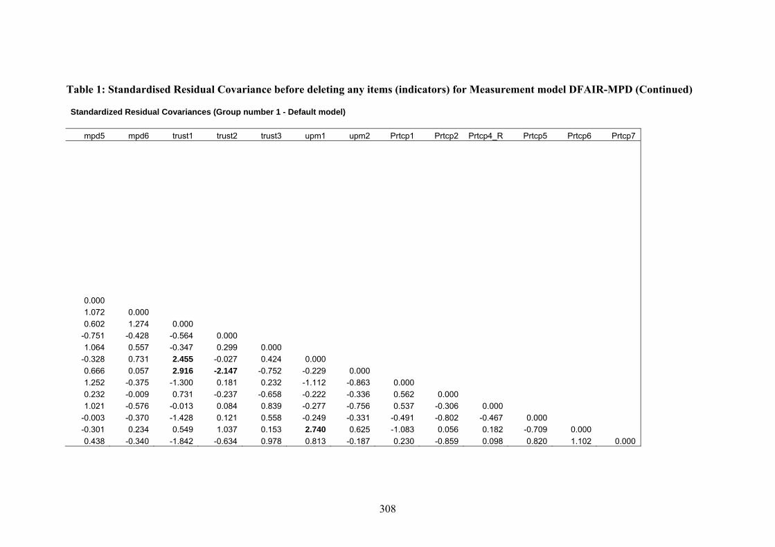
308

Table 1: Standardised Residual Covariance before deleting any items (indicators) for Measurement model DFAIR-MPD (Continued) Standardized Residual Covariances (Group number 1 - Default model)

mpd5 mpd6 trust1 trust2 trust3 upm1 upm2 Prtcp1 Prtcp2 Prtcp4_R Prtcp5 Prtcp6 Prtcp7

0 . 000 1.072 0.000 0.602 1.274 0.000

-0.751 -0.428 -0.564 0.000 1.064 0.557 -0.347 0.299 0.000

-0.328 0.731 2.455 -0.027 0.424 0.000 0.666 0.057 2.916 -2.147 -0.752 -0.229 0.000 1.252 -0.375 -1.300 0.181 0.232 -1.112 -0.863 0.000 0.232 -0.009 0.731 -0.237 -0.658 -0.222 -0.336 0.562 0.000 1.021 -0.576 -0.013 0.084 0.839 -0.277 -0.756 0.537 -0.306 0.000

-0.003 -0.370 -1.428 0.121 0.558 -0.249 -0.331 -0.491 -0.802 -0.467 0.000 -0.301 0.234 0.549 1.037 0.153 2.740 0.625 -1.083 0.056 0.182 -0.709 0.000 0.438 -0.340 -1.842 -0.634 0.978 0.813 -0.187 0.230 -0.859 0.098 0.820 1.102 0.000

Table 2: Modification Indices (MIs) of Regression Weights before deleting any Indicators for measurement model of DFAIR-MPD Regression Weights: (Group number 1 - Default model)

M.I.Par

Changedf1 <--- Prtcp6 5.193 -0.113df2 <--- mpd5 6.294 -0.2mpd8 <--- trust2 4.856 -0.159mpd7 <--- upm2 4.558 0.096trust5 <--- mpd6 5.088 -0.278upm3 <--- trust1 9.874 0.168Prtcp10 <--- Prtcp2 4.482 0.116mpd2 <--- mpd5 5.334 -0.17mpd2 <--- Prtcp5 4.531 0.113mpd4 <--- trust5 4.544 0.094mpd4 <--- Prtcp10 6.246 0.145mpd5 <--- mpd2 7.447 -0.172trust1 <--- CMB 21.34 0.392trust1 <--- mpd8 4.01 0.137trust1 <--- upm3 28.96 0.352trust1 <--- upm1 8.395 0.202trust1 <--- upm2 20.336 0.226trust1 <--- Prtcp5 4.68 -0.145trust1 <--- Prtcp7 6.29 -0.175trust2 <--- mpd8 12.861 -0.187trust2 <--- upm2 9.972 -0.121trust3 <--- mpd5 4.062 0.142trust3 <--- Prtcp7 7.16 0.141upm1 <--- Prtcp6 5.034 0.14upm2 <--- mpd7 9.417 0.278upm2 <--- trust2 5.396 -0.209Prtcp2 <--- Prtcp10 4.15 0.122Prtcp5 <--- df2 6.259 0.175Prtcp5 <--- mpd2 5.908 0.207Prtcp6 <--- CMB 7.228 0.201Prtcp6 <--- upm3 6.696 0.149Prtcp6 <--- upm1 11.522 0.208Prtcp7 <--- trust1 6.445 -0.132

309

Table 3: Standarised Residual Covariance after deleting seven items (indicators) for Measurement model DFAIR-MPD Standardized Residual Covariances (Group number 1 - Default model)

df1 df2 mpd1 mpd2 mpd3 mpd5 mpd7 mpd9 trust2 trust3 trust5 upm1

df1 . 0 0 00 df2 0.000 0.000 mpd1 -0.249 -1.082 0.000 mpd2 0.192 1.029 0.073 0.000 mpd3 0.834 -0.501 0.057 0.355 0.000 mpd5 0.505 -1.625 0.118 -1.946 0.162 0.000 mpd7 0.561 -1.221 0.348 0.924 -0.799 0.482 0.000 mpd9 -0.412 -0.031 -0.081 0.667 0.298 -0.451 -0.087 0.000 trust2 0.192 -0.072 -0.942 0.048 0.559 -0.564 -0.625 -1.002 0.000 trust3 -0.088 -0.135 -0.777 -0.222 1.075 1.256 -0.057 -0.936 -0.020 0.000 trust5 0.541 0.577 -0.193 -1.447 -0.885 -1.207 0.136 -1.292 0.815 -0.310 0.000 upm1 -0.192 0.573 0.672 -1.537 -0.166 0.073 -0.769 -1.325 -0.103 0.309 -0.616 0.000upm3 0.006 -0.219 -0.495 -0.130 0.562 1.408 0.767 -0.269 -0.227 -0.021 -1.179 0.000Prtcp2 0.539 0.756 0.128 -0.052 0.729 0.394 0.928 0.768 -0.175 -0.624 -1.534 -0.364Prtcp4_R -0.769 -0.593 -0.482 -1.186 -0.004 1.205 1.035 -1.002 0.173 0.901 0.065 -0.409Prtcp5 1.033 1.702 -1.048 1.701 0.225 0.023 -0.807 0.699 -0.007 0.387 -0.548 -0.482Prtcp7 -0.381 -0.299 -1.596 -0.085 0.155 0.622 -0.834 -0.275 -0.544 1.044 -0.958 0.681Prtcp8 0.323 -0.442 -0.543 -0.619 -0.050 -1.032 0.170 -0.473 -0.050 -0.470 0.303 0.314Prtcp10 -0.364 -0.641 -1.203 0.475 0.805 0.235 0.455 -0.242 -0.494 -0.220 -1.462 -1.017

310

Table 3: Standarised Residual Covariance after deleting seven items (indicators) for Measurement model DFAIR-MPD (Continued) Standardized Residual Covariances (Group number 1 - Default model)

upm3 Prtcp2 Prtcp4_R Prtcp5 Prtcp7 Prtcp8 Prtcp10

0.000 1.306 0.000 0.500 -0.148 0.000

-0.171 -0.917 -0.559 0.000 0.083 -0.700 0.297 0.730 0.000

-0.329 -0.276 -0.047 0.663 0.437 0.000 0.099 1.244 0.382 -0.804 -0.317 -0.282 0.000

311

Table 4: Implied (for all variables) Correlations for Measurement model DFAIR - MPD Implied (for all variables) Correlations (Group number 1 - Default model)

DFAIR MPD TRST CMB PRTCPT df1 df2 mpd1 mpd2 mpd3 mpd5 mpd7 mpd9 DF AIR . 01 00 MPD 0.368 1.000 TRST 0.796 0.348 1.000 CMB 0.493 0.355 0.563 1.000 PRTCPT 0.764 0.546 0.674 0.379 1.000 df1 0.808 0.298 0.643 0.398 0.617 1.000 df2 0.652 0.240 0.519 0.321 0.498 0.527 1.000 mpd1 0.243 0.660 0.230 0.234 0.360 0.196 0.158 1.000 mpd2 0.167 0.452 0.158 0.161 0.247 0.135 0.109 0.298 1.000 mpd3 0.279 0.758 0.264 0.269 0.414 0.226 0.182 0.500 0.343 1.000 mpd5 0.221 0.601 0.209 0.213 0.328 0.179 0.144 0.396 0.272 0.455 1.000 mpd7 0.233 0.634 0.221 0.225 0.346 0.189 0.152 0.418 0.287 0.481 0.381 1.000 mpd9 0.175 0.474 0.165 0.168 0.259 0.141 0.114 0.313 0.214 0.360 0.285 0.301 1.000 trust5 0.235 0.103 0.296 0.166 0.199 0.190 0.153 0.068 0.047 0.078 0.062 0.065 0.049 trust3 0.700 0.306 0.879 0.495 0.593 0.566 0.456 0.202 0.139 0.232 0.184 0.194 0.145 trust2 0.639 0.280 0.803 0.452 0.542 0.517 0.417 0.185 0.127 0.212 0.168 0.177 0.133 upm3 0.382 0.276 0.437 0.776 0.294 0.309 0.249 0.182 0.125 0.209 0.166 0.175 0.131 upm1 0.399 0.288 0.456 0.810 0.307 0.322 0.260 0.190 0.130 0.218 0.173 0.182 0.136 Prtcp2 0.541 0.387 0.477 0.268 0.708 0.437 0.352 0.255 0.175 0.293 0.232 0.245 0.183 Prtcp4_R 0.553 0.395 0.488 0.275 0.724 0.447 0.360 0.261 0.179 0.300 0.237 0.251 0.187 Prtcp5 0.496 0.355 0.438 0.246 0.649 0.401 0.323 0.234 0.160 0.269 0.213 0.225 0.168 Prtcp7 0.551 0.394 0.486 0.274 0.721 0.445 0.359 0.260 0.178 0.299 0.237 0.250 0.187 Prtcp8 0.546 0.391 0.482 0.271 0.715 0.441 0.356 0.258 0.177 0.296 0.235 0.248 0.185 Prtcp10 0.564 0.403 0.498 0.280 0.738 0.456 0.367 0.266 0.182 0.306 0.242 0.255 0.191

312

313

Table 4: Implied (for all variables) Correlations for Measurement model DFAIR – MPD (Continued) Implied (for all variables) Correlations (Group number 1 - Default model)

trust5 trust3 trust2 upm3 upm1 Prtcp2 Prtcp4_R Prtcp5 Prtcp7 Prtcp8 Prtcp10

1. 00 0 0.260 1.000 0.237 0.706 1.000 0.129 0.384 0.351 1.000 0.135 0.401 0.366 0.628 1.000 0.141 0.420 0.383 0.208 0.217 1.000 0.144 0.429 0.392 0.213 0.222 0.512 1.000 0.129 0.385 0.351 0.191 0.199 0.459 0.470 1.000 0.144 0.428 0.391 0.212 0.222 0.511 0.522 0.468 1.000 0.142 0.424 0.387 0.211 0.220 0.506 0.518 0.464 0.516 1.000 0.147 0.438 0.400 0.217 0.227 0.522 0.534 0.479 0.532 0.528 1.000

APPENDIX II

PART D


VALIDITY FOR DFAIR – MPS MODEL

314

Table 1: Standardised Residual Covariance before deleting any items (indicators) for Measurement model DFAIR-MPS Standardized Residual Covariances (Group number 1 - Default model)

df1 df2 mps1 mps2 mps3 trust5 upm3 Prtcp10 Prtcp8 trust1 trust2 trust3 upm1 df1 . 0 0 00 df2 0.000 0.000 mps1 -0.339 0.009 0.000 mps2 -0.445 1.194 -0.082 0.000 mps3 -0.045 0.253 0.096 -0.016 0.000 trust5 0.611 0.644 -2.265 -0.137 -0.729 0.000 upm3 -0.205 -0.373 0.318 0.891 -0.103 -1.412 0.000 Prtcp10 -0.264 -0.534 0.005 -0.475 -0.216 -1.383 -0.226 0.000 Prtcp8 0.386 -0.368 -0.327 -0.214 0.311 0.368 -0.664 -0.205 0.000 trust1 0.001 -0.513 3.383 3.667 2.963 -1.157 3.573 0.716 -0.506 0.000 trust2 0.179 -0.056 -1.481 -0.492 -0.763 1.054 -0.975 -0.436 -0.026 -0.653 0.000 trust3 -0.062 -0.084 -1.393 0.348 -0.760 -0.036 -0.799 -0.124 -0.412 -0.444 0.400 0.000 upm1 0.419 1.094 -1.576 0.287 -1.456 -0.474 -0.049 -0.730 0.581 2.484 0.135 0.599 0.000 upm2 -0.204 0.324 0.207 0.372 -0.272 0.110 0.048 -0.321 -0.812 2.938 -2.015 -0.605 0.062 Prtcp1 0.092 1.039 -0.512 -0.727 0.126 0.373 -1.008 -0.543 -0.284 -1.335 0.253 0.309 -1.017 Prtcp2 0.593 0.825 -0.193 -0.606 -0.752 -1.473 0.961 1.315 -0.251 0.682 -0.157 -0.574 -0.107 Prtcp4_R -0.801 -0.596 0.430 0.141 0.480 0.099 0.102 0.350 -0.120 -0.108 0.111 0.868 -0.189 Prtcp5 1.226 1.885 -0.251 0.084 0.088 -0.445 -0.403 -0.586 0.847 -1.517 0.132 0.569 -0.180 Prtcp6 -1.147 0.786 0.572 0.378 0.145 0.420 1.943 0.121 -0.179 0.429 1.009 0.122 2.787 Prtcp7 -0.483 -0.360 0.567 0.542 0.175 -0.949 -0.353 -0.429 0.282 -1.980 -0.666 0.940 0.869

315

316

Table 1: Standardised Residual Covariance before deleting any items (indicators) for Measurement model DFAIR-MPS (Continued) Standardized Residual Covariances (Group number 1 - Default model)

upm2 Prtcp1 Prtcp2 Prtcp4_R Prtcp5 Prtcp6 Prtcp7

0.000 -0.780 0.000 -0.237 0.691 0.000 -0.682 0.610 -0.229 0.000 -0.272 -0.443 -0.751 -0.476 0.000 0.663 -1.077 0.057 0.123 -0.773 0.000

-0.141 0.238 -0.857 0.029 0.741 0.973 0.000

Table 2: Modification Indices (MIs) of Regression Weights before deleting any Indicators for measurement model of DFAIR-MPS Regression Weights: (Group number 1 - Default model)

M.I.Par

Changedf1 <--- Prtcp6 5.472 -0.116mps1 <--- trust5 11.153 -0.148mps1 <--- trust3 4.924 -0.11mps2 <--- CMB 5.848 0.148mps2 <--- df2 4.639 0.113mps2 <--- trust5 4.516 0.089mps2 <--- trust3 6.944 0.123mps2 <--- upm1 11.892 0.17mps3 <--- upm1 5.904 -0.115trust5 <--- mps1 4.779 -0.16upm3 <--- trust1 5.259 0.119Prtcp10 <--- Prtcp2 5.295 0.128trust1 <--- MPS 24.072 0.294trust1 <--- CMB 24.588 0.423trust1 <--- mps1 27.372 0.294trust1 <--- mps2 20.995 0.243trust1 <--- mps3 18.24 0.231trust1 <--- upm3 27.547 0.34trust1 <--- upm1 8.204 0.197trust1 <--- upm2 19.757 0.221trust1 <--- Prtcp5 5.432 -0.155trust1 <--- Prtcp7 7.143 -0.184trust2 <--- upm2 10.054 -0.122trust3 <--- mps1 4.595 -0.093trust3 <--- Prtcp7 7.3 0.144upm1 <--- mps1 5.45 -0.113upm1 <--- Prtcp6 5.155 0.143upm2 <--- trust2 4.192 -0.186Prtcp2 <--- Prtcp10 4.844 0.133Prtcp5 <--- df2 5.98 0.171Prtcp6 <--- CMB 7.092 0.201Prtcp6 <--- upm3 6.486 0.146Prtcp6 <--- upm1 11.186 0.204Prtcp7 <--- trust1 7.52 -0.142

317

Table 3: Standarised Residual Covariance after deleting five items (indicators) for Measurement model DFAIR-MPS Standardized Residual Covariances (Group number 1 - Default model)

df1 df2 mps2 mps3 trust2 trust3 trust5 upm1 upm3 Prtcp2 Prtcp4_Rdf1 0.000 df2 0.000 0.000 mps2 -0.340 1.342 0.000 mps3 0.665 0.875 0.000 0.000 trust2 0.199 0.108 -0.460 0.140 0.000 trust3 -0.174 -0.018 0.297 0.149 -0.015 0.000 trust5 0.530 0.637 -0.176 -0.436 0.844 -0.326 0.000 upm1 0.062 0.892 -0.612 -1.197 0.263 0.644 -0.484 0.000 upm3 -0.195 -0.269 0.393 0.671 -0.366 -0.242 -1.242 0.000 0.000 Prtcp2 0.577 0.940 -0.297 0.139 -0.074 -0.587 -1.505 -0.198 1.154 0.000 Prtcp4_R -0.807 -0.472 0.472 1.427 0.209 0.865 0.069 -0.277 0.305 -0.053 0.000Prtcp5 0.983 1.807 0.258 0.811 0.014 0.342 -0.549 -0.371 -0.352 -0.847 -0.564Prtcp7 -0.491 -0.236 0.877 1.127 -0.572 0.935 -0.980 0.776 -0.150 -0.686 0.224Prtcp8 0.234 -0.362 0.036 1.173 -0.059 -0.553 0.289 0.420 -0.547 -0.237 -0.093Prtcp10 -0.368 -0.490 -0.197 0.678 -0.428 -0.223 -1.447 -0.868 -0.079 1.385 0.433

318

Table 3: Standarised Residual Covariance after deleting five items (indicators) for Measurement model DFAIR-MPS (Continued) Standardized Residual Covariances (Group number 1 - Default model)

Prtcp5 Prtcp7 Prtcp8 Prtcp10

0.000 0.646 0.000 0.604 0.307 0.000

-0.775 -0.351 -0.290 0.000

319

Table 4: Implied (for all variables) Correlations for Measurement model DFAIR - MPS Implied (for all variables) Correlations (Group number 1 - Default model)

DFAIR MPS TRST CMB PRTCPT df1 df2 mps2 mps3 trust5 trust3 trust2 upm3 DF AIR . 01 00 MPS 0.234 1.000 TRST 0.787 0.359 1.000 CMB 0.480 0.521 0.552 1.000 PRTCPT 0.756 0.266 0.675 0.384 1.000 df1 0.823 0.192 0.648 0.395 0.622 1.000 df2 0.640 0.150 0.504 0.307 0.484 0.527 1.000 mps2 0.245 1.047 0.376 0.546 0.279 0.201 0.157 1.000 mps3 0.190 0.813 0.292 0.424 0.216 0.156 0.122 0.851 1.000 trust5 0.232 0.106 0.295 0.163 0.199 0.191 0.149 0.111 0.086 1.000 trust3 0.697 0.318 0.886 0.489 0.598 0.573 0.446 0.333 0.259 0.261 1.000 trust2 0.627 0.287 0.797 0.440 0.538 0.516 0.402 0.300 0.233 0.235 0.706 1.000 upm3 0.396 0.429 0.455 0.824 0.316 0.326 0.253 0.450 0.349 0.134 0.403 0.363 1.000 upm1 0.366 0.398 0.421 0.763 0.293 0.301 0.235 0.416 0.323 0.124 0.373 0.336 0.628 Prtcp2 0.527 0.186 0.470 0.267 0.697 0.434 0.337 0.194 0.151 0.139 0.416 0.375 0.220 Prtcp4_R 0.547 0.193 0.488 0.278 0.723 0.450 0.350 0.202 0.157 0.144 0.432 0.389 0.229 Prtcp5 0.492 0.173 0.439 0.250 0.650 0.405 0.315 0.181 0.141 0.129 0.389 0.350 0.206 Prtcp7 0.553 0.195 0.493 0.281 0.731 0.455 0.354 0.204 0.158 0.145 0.437 0.393 0.231 Prtcp8 0.546 0.192 0.487 0.277 0.721 0.449 0.349 0.201 0.156 0.144 0.431 0.388 0.228 Prtcp10 0.554 0.195 0.494 0.281 0.733 0.456 0.355 0.204 0.159 0.146 0.438 0.394 0.232

320

321

Table 4: Implied (for all variables) Correlations for Measurement model DFAIR – MPS (Continued) Implied (for all variables) Correlations (Group number 1 - Default model)


1.000 0.204 1.000 0.212 0.504 1.000 0.190 0.453 0.470 1.000 0.214 0.509 0.529 0.475 1.000 0.211 0.503 0.522 0.469 0.527 1.000 0.214 0.511 0.530 0.476 0.536 0.529 1.000

APPENDIX III

PART A

STANDARDISED RESIDUAL COVARIANCE AND IMPLIED CORRELATIONS FOR MODEL ANALYSIS

FOR PFAIR – MPD MODEL

322

Table 1: Standardised Residual Covariance before deleting any items (indicators) for Model Analysis for PFAIR-MPD Model Standardized Residual Covariances (Group number 1 - Default model)

mpd9 trust2 trust3 trust5 pf8 pf7 pf6 pf5 mpd7 mpd5 mpd3 mpd2 mpd1 m p . 4d9 0 00 trust2 -0.832 0.000 trust3 -0.714 -0.026 0.000 trust5 -1.230 0.741 -0.318 0.000 pf8 -0.577 0.435 0.520 1.150 0.000 pf7 -0.998 0.429 -0.517 -1.595 1.034 0.000 pf6 -0.451 -0.016 -0.082 0.437 0.020 -0.353 0.000 pf5 -0.257 -0.268 0.054 0.573 -0.357 -0.227 0.771 0.000 mpd7 -0.079 -0.418 0.219 0.212 -0.817 0.174 -0.066 0.532 0.007 mpd5 -0.414 -0.352 1.540 -1.130 0.318 0.995 -1.512 0.078 0.483 0.006 mpd3 0.362 0.840 1.443 -0.784 -0.389 1.484 -0.993 -0.460 -0.776 0.231 0.010 mpd2 0.710 0.218 -0.003 -1.386 -1.717 -0.539 -0.554 -0.671 0.945 -1.901 0.432 0.004 mpd1 -0.111 -0.749 -0.516 -0.122 -0.075 0.997 -1.493 -0.504 0.257 0.072 0.025 0.057 0.008 upm3 -0.468 1.599 2.041 -0.500 0.587 1.530 -0.020 -1.294 0.474 1.148 0.252 -0.314 -0.820 upm1 -1.252 2.206 2.908 0.242 1.474 2.783 0.535 -0.202 -0.693 0.164 -0.042 -1.462 0.730 Prtcp2 1.274 -0.231 -0.577 -1.559 -0.432 0.838 -0.508 -0.360 1.578 1.025 1.537 0.433 0.769 Prtcp4_R -0.540 0.002 0.829 -0.005 -0.712 -1.106 -0.033 -0.141 1.640 1.801 0.738 -0.740 0.103 Prtcp5 1.141 -0.115 0.372 -0.592 0.684 -0.117 0.582 0.428 -0.256 0.572 0.927 2.133 -0.501 Prtcp7 0.158 -0.788 0.885 -1.058 -1.185 -0.377 0.373 0.159 -0.293 1.170 0.848 0.336 -1.069 Prtcp8 -0.020 -0.234 -0.556 0.227 -0.740 0.582 -0.106 -0.146 0.749 -0.472 0.674 -0.181 0.025 Prtcp10 0.257 -0.607 -0.230 -1.510 -0.109 -0.048 0.037 -1.007 1.097 0.863 1.612 0.962 -0.584

323

324

Table 1: Standardised Residual Covariance before deleting any items (indicators) for Model Analysis for PFAIR-MPD Model (Continued) Standardized Residual Covariances (Group number 1 - Default model)

upm3 upm1 Prtcp2 Prtcp4_R Prtcp5 Prtcp7 Prtcp8 Prtcp10

0.000 0.018 0.000 0.756 -0.448 0.000

-0.129 -0.562 -0.018 0.000 -0.701 -0.593 -0.746 -0.507 0.000 -0.593 0.476 -0.665 0.191 0.691 0.000 -0.953 0.151 -0.167 -0.073 0.697 0.312 0.000 -0.498 -1.137 1.456 0.449 -0.688 -0.349 -0.238 0.000

Table 2: Modification Indices (MIs) of Regression Weights before deleting any Indicators for Analysis Model of PFAIR-MPD Regression Weights: (Group number 1 - Default model)

M.I.Par

ChangeTRST <--- CMB 8.998 0.105CMB <--- TRST 5.71 0.449trust3 <--- CMB 5.639 0.194trust3 <--- mpd5 6.456 0.185trust3 <--- upm1 5.968 0.133trust3 <--- Prtcp7 5.228 0.125pf7 <--- CMB 6.499 0.188pf7 <--- trust5 4.188 -0.085pf7 <--- upm1 9.421 0.151pf6 <--- MPD 4.522 -0.258pf6 <--- mpd5 8.445 -0.202pf6 <--- mpd3 5.266 -0.153pf5 <--- CMB 4.078 -0.207pf5 <--- upm3 4.867 -0.141mpd5 <--- mpd2 6.719 -0.168mpd2 <--- mpd5 5.065 -0.166mpd2 <--- Prtcp5 4.583 0.114upm1 <--- TRST 4.061 0.372upm1 <--- trust3 4.752 0.125upm1 <--- pf7 5.857 0.182Prtcp2 <--- Prtcp10 5.612 0.146Prtcp5 <--- mpd2 7.453 0.23Prtcp10 <--- Prtcp2 6.438 0.141

325

Table 3: Standardised Residual Covariance after deleting one item (indicator) for Model Analysis for PFAIR-MPD Model Standardized Residual Covariances (Group number 1 - Default model)

trust2 trust3 trust5 pf8 pf7 pf6 pf5 mpd9 mpd7 mpd5 mpd3 mpd1tr us . 0t2 0 00 trust3 -0.026 0.000 trust5 0.737 -0.318 0.000 pf8 0.420 0.509 1.145 0.000 pf7 0.418 -0.523 -1.600 1.012 0.000 pf6 -0.010 -0.070 0.439 0.013 -0.352 0.000 pf5 -0.274 0.054 0.571 -0.374 -0.239 0.778 0.000 mpd9 -0.796 -0.674 -1.216 -0.564 -0.979 -0.423 -0.235 0.003 mpd7 -0.381 0.261 0.226 -0.812 0.185 -0.045 0.546 0.080 0.006 mpd5 -0.455 1.431 -1.168 0.178 0.818 -1.687 -0.094 -0.508 0.333 0.006 mpd3 0.872 1.481 -0.772 -0.395 1.480 -0.985 -0.459 0.528 -0.596 0.030 0.008 mpd1 -0.747 -0.511 -0.121 -0.108 0.958 -1.522 -0.538 -0.009 0.364 -0.170 0.118 0.007upm3 1.603 2.049 -0.498 0.587 1.534 -0.006 -1.287 -0.488 0.434 0.932 0.189 -0.908upm1 2.187 2.890 0.235 1.456 2.763 0.523 -0.219 -1.285 -0.750 -0.048 -0.123 0.626Prtcp2 -0.234 -0.575 -1.560 -0.440 0.835 -0.494 -0.358 1.293 1.589 0.865 1.535 0.735Prtcp4_R -0.005 0.828 -0.007 -0.723 -1.113 -0.022 -0.143 -0.523 1.650 1.630 0.735 0.067Prtcp5 -0.112 0.381 -0.591 0.681 -0.115 0.602 0.436 1.160 -0.242 0.428 0.929 -0.528Prtcp7 -0.790 0.889 -1.059 -1.193 -0.379 0.389 0.162 0.178 -0.281 1.001 0.847 -1.102Prtcp8 -0.237 -0.554 0.225 -0.749 0.579 -0.092 -0.144 -0.001 0.761 -0.634 0.672 -0.009Prtcp10 -0.608 -0.225 -1.510 -0.117 -0.050 0.054 -1.003 0.277 1.110 0.696 1.612 -0.617

326

327

Table 3: Standardised Residual Covariance after deleting one item (indicator) for Model Analysis for PFAIR-MPD Model (Continued) Standardized Residual Covariances (Group number 1 - Default model)

upm3 upm1 Prtcp2 Prtcp4_R Prtcp5 Prtcp7 Prtcp8 Prtcp10

0.000 0.019 0.000 0.763 -0.469 0.000

-0.125 -0.586 -0.024 0.000 -0.692 -0.609 -0.741 -0.505 0.000 -0.586 0.455 -0.666 0.187 0.699 0.000 -0.947 0.129 -0.168 -0.079 0.703 0.312 0.000 -0.490 -1.157 1.457 0.446 -0.681 -0.347 -0.237 0.000

APPENDIX III

PART B


FOR PFAIR – MPS MODEL

328

Table 1: Standardised Residual Covariance before deleting any items (indicators) for Model Analysis for PFAIR-MPS Model Standardized Residual Covariances (Group number 1 - Default model)

trust2 trust3 trust5 pf8 pf7 pf6 pf5 mps3 mps2 mps1 upm3 upm1tr us . 0t2 0 00 trust3 -0.018 0.000 trust5 0.771 -0.311 0.000 pf8 0.483 0.539 1.171 0.000 pf7 0.601 -0.379 -1.528 1.069 0.000 pf6 -0.087 -0.201 0.411 -0.177 -0.458 0.000 pf5 -0.233 0.051 0.590 -0.447 -0.213 0.488 0.000 mps3 0.567 0.701 -0.274 -1.170 0.122 0.756 0.111 0.095 mps2 0.837 1.837 0.320 -0.631 0.368 0.270 -0.557 0.086 0.092 mps1 -0.249 -0.038 -1.849 -0.998 0.107 -0.011 -1.135 0.179 0.023 0.083 upm3 1.602 2.022 -0.497 0.638 1.658 -0.024 -1.243 -0.228 0.783 0.205 0.000 upm1 2.666 3.389 0.409 1.877 3.357 1.040 0.300 -0.978 0.799 -1.123 0.009 0.000Prtcp2 -0.201 -0.584 -1.545 -0.320 1.094 -0.489 -0.243 -0.411 -0.261 0.135 0.765 0.101Prtcp4_R -0.004 0.780 -0.005 -0.626 -0.891 -0.055 -0.057 0.809 0.470 0.741 -0.145 -0.008Prtcp5 -0.103 0.348 -0.586 0.778 0.100 0.582 0.523 0.297 0.296 -0.055 -0.704 -0.091Prtcp7 -0.791 0.840 -1.057 -1.096 -0.150 0.354 0.248 0.499 0.873 0.877 -0.607 1.049Prtcp8 -0.222 -0.583 0.234 -0.640 0.826 -0.107 -0.044 0.584 0.058 -0.075 -0.957 0.716Prtcp10 -0.598 -0.261 -1.504 -0.010 0.190 0.032 -0.910 0.078 -0.180 0.286 -0.504 -0.577

329

330

Table 1: Standardised Residual Covariance before deleting any items (indicators) for Model Analysis for PFAIR-MPS Model (Continued) Standardized Residual Covariances (Group number 1 - Default model)


0.000 -0.018 0.000 -0.726 -0.527 0.000 -0.661 0.149 0.675 0.000 -0.145 -0.096 0.698 0.293 0.000 1.475 0.421 -0.691 -0.372 -0.242 0.000

Table 2: Modification Indices (MIs) of Regression Weights before deleting any Indicators for Analysis Model of PFAIR-MPS


M.I. Par Change TRST <--- CMB 8.110 .104 CMB <--- TRST 4.453 .339 trust3 <--- CMB 4.610 .184 trust3 <--- mps2 4.320 .088 trust3 <--- upm1 6.349 .137 trust3 <--- Prtcp7 4.610 .117 pf7 <--- CMB 5.401 .183 pf7 <--- trust5 4.236 -.087 pf7 <--- upm3 4.653 .101 pf7 <--- upm1 10.127 .159 pf5 <--- CMB 4.512 -.228 pf5 <--- upm3 4.742 -.139 mps3 <--- upm1 5.574 -.111 mps2 <--- CMB 4.299 .162 mps2 <--- trust3 7.672 .130 mps2 <--- trust5 4.621 .090 mps2 <--- upm1 12.409 .174 mps1 <--- TRST 4.025 -.322 mps1 <--- trust3 4.482 -.105 mps1 <--- trust5 10.951 -.147 upm1 <--- PFAIR 4.777 .187 upm1 <--- TRST 7.042 .495 upm1 <--- trust2 4.761 .135 upm1 <--- trust3 7.521 .158 upm1 <--- pf7 9.156 .230 Prtcp2 <--- Prtcp10 5.713 .147 Prtcp10 <--- Prtcp2 6.632 .144

331

Table 3: Standardised Residual Covariance after deleting one item (indicator) for Model Analysis for PFAIR-MPS Model Standardized Residual Covariances (Group number 1 - Default model)

trust2 trust3 trust5 pf8 pf6 pf5 mps3 mps2 mps1 upm3 upm1 Prtcp2tr us . 0t2 0 00 trust3 -0.009 0.000 trust5 0.804 -0.352 0.000 pf8 0.836 0.829 1.286 0.000 pf6 -0.105 -0.351 0.374 -0.079 0.000 pf5 -0.141 0.032 0.600 -0.259 0.138 0.000 mps3 0.615 0.689 -0.269 -1.109 0.571 0.004 0.068 mps2 0.886 1.826 0.325 -0.569 0.093 -0.658 0.057 0.065 mps1 -0.202 -0.047 -1.842 -0.940 -0.180 -1.231 0.147 0.000 0.059 upm3 1.699 2.062 -0.475 0.868 0.031 -1.135 -0.286 0.728 0.151 0.000 upm1 2.764 3.449 0.435 2.064 1.112 0.407 -0.965 0.814 -1.109 0.007 0.000 Prtcp2 -0.099 -0.588 -1.529 0.048 -0.467 -0.116 -0.419 -0.267 0.128 0.877 0.213 0.000Prtcp4_R 0.001 0.662 -0.029 -0.318 -0.147 -0.027 0.742 0.408 0.680 -0.099 0.061 -0.021Prtcp5 -0.057 0.288 -0.591 1.092 0.545 0.593 0.261 0.263 -0.088 -0.636 -0.010 -0.680Prtcp7 -0.762 0.746 -1.072 -0.771 0.287 0.303 0.445 0.821 0.827 -0.545 1.131 -0.636Prtcp8 -0.136 -0.609 0.242 -0.276 -0.107 0.068 0.563 0.041 -0.092 -0.859 0.823 -0.052Prtcp10 -0.534 -0.313 -1.505 0.348 0.006 -0.822 0.045 -0.209 0.255 -0.418 -0.480 1.546

332

333

Table 3: Standardised Residual Covariance after deleting one item (indicator) for Model Analysis for PFAIR-MPS Model (Continued) Standardized Residual Covariances (Group number 1 - Default model) Prtcp4_R Prtcp5 Prtcp7 Prtcp8 Prtcp10

0.000 -0.593 0.000 0.044 0.633 0.000

-0.126 0.723 0.292 0.000 0.362 -0.693 -0.402 -0.199 0.000

APPENDIX III

PART C


FOR DFAIR – MPD MODEL

334

Table 1: Standardised Residual Covariance before deleting any items (indicators) for Model Analysis for DFAIR-MPD Model Standardized Residual Covariances (Group number 1 - Default model)

mpd9 trust2 trust3 trust5 df2 df1 mpd7 mpd5 mpd3 mpd2 mpd1 upm3m p . 5d9 -0 01 trust2 -0.776 0.000 trust3 -0.636 0.071 0.000 trust5 -1.229 0.626 -0.398 0.000 df2 -0.170 -0.289 -0.186 0.408 0.000 df1 -0.593 -0.101 -0.182 0.319 1.336 0.000 mpd7 -0.138 -0.321 0.348 0.220 -1.398 0.320 -0.027 mpd5 -0.479 -0.266 1.656 -1.122 -1.781 0.290 0.449 -0.024 mpd3 0.257 0.935 1.574 -0.779 -0.703 0.561 -0.838 0.150 -0.039 mpd2 0.613 0.260 0.060 -1.389 0.888 0.009 0.857 -1.982 0.298 -0.014 mpd1 -0.119 -0.619 -0.351 -0.102 -1.258 -0.484 0.305 0.103 0.034 0.021 -0.029 upm3 -0.609 1.599 2.075 -0.536 0.574 0.969 0.313 0.987 0.040 -0.463 -0.946 0.000upm1 -1.352 2.239 2.973 0.221 1.804 1.290 -0.801 0.053 -0.193 -1.569 0.646 0.001Prtcp2 0.782 -0.361 -0.654 -1.679 0.624 0.352 0.951 0.432 0.773 -0.047 0.165 0.678Prtcp4_R -0.963 0.028 0.920 -0.067 -0.680 -0.901 1.089 1.272 0.077 -1.159 -0.413 -0.100Prtcp5 0.719 -0.165 0.375 -0.677 1.592 0.875 -0.775 0.068 0.278 1.711 -1.003 -0.724Prtcp7 -0.244 -0.700 1.046 -1.095 -0.400 -0.531 -0.789 0.680 0.224 -0.065 -1.537 -0.521Prtcp8 -0.441 -0.205 -0.466 0.166 -0.540 0.174 0.215 -0.972 0.021 -0.598 -0.483 -0.923Prtcp10 -0.195 -0.623 -0.186 -1.589 -0.715 -0.482 0.521 0.314 0.899 0.510 -1.123 -0.497

335

336

Table 1: Standardised Residual Covariance before deleting any items (indicators) for Model Analysis for DFAIR-MPD Model (Continued) Standardized Residual Covariances (Group number 1 - Default model)


0.000 -0.478 0.000 -0.497 -0.129 0.000 -0.578 -0.932 -0.522 0.000 0.582 -0.699 0.356 0.750 0.000 0.218 -0.272 0.014 0.686 0.480 0.000

-1.097 1.284 0.482 -0.750 -0.239 -0.202 0.000

Table 2: Modification Indices (MIs) of Regression Weights before deleting any Indicators for Analysis Model of DFAIR-MPD


M.I. Par Change TRST <--- CMB 4.995 .065 CMB <--- TRST 5.887 .435 trust3 <--- CMB 5.169 .185 trust3 <--- mpd5 8.676 .212 trust3 <--- upm1 5.681 .129 trust3 <--- Prtcp7 6.583 .139 df2 <--- mpd5 6.643 -.212 df1 <--- df2 4.754 .110 mpd5 <--- mpd2 7.111 -.172 mpd2 <--- mpd5 5.412 -.170 mpd2 <--- Prtcp5 4.021 .106 upm1 <--- TRST 4.094 .359 upm1 <--- trust3 4.908 .127 upm1 <--- df2 4.005 .129 Prtcp2 <--- Prtcp10 4.725 .131 Prtcp5 <--- df2 5.423 .160 Prtcp5 <--- mpd2 5.553 .198 Prtcp10 <--- Prtcp2 5.117 .126

337

Table 3: Standardised Residual Covariance after deleting one item (indicator) for Model Analysis for DFAIR-MPD Model Standardized Residual Covariances (Group number 1 - Default model)

mpd9 trust2 trust3 trust5 df2 df1 mpd7 mpd5 mpd3 mpd2 mpd1 upm3m p . 2d9 -0 01 trust2 -0.875 0.000 trust3 -0.765 -0.009 0.000 trust5 -1.258 0.690 -0.380 0.000 df2 0.031 -0.098 -0.062 0.520 0.000 df1 -0.352 0.100 -0.065 0.446 0.000 0.000 mpd7 -0.142 -0.460 0.167 0.179 -1.141 0.635 -0.022 mpd5 -0.496 -0.405 1.475 -1.164 -1.546 0.579 0.412 -0.019 mpd3 0.259 0.771 1.361 -0.826 -0.393 0.940 -0.855 0.114 -0.030 mpd2 0.622 0.165 -0.064 -1.416 1.084 0.243 0.858 -1.995 0.304 -0.011 mpd1 -0.070 -0.734 -0.506 -0.133 -0.966 -0.130 0.352 0.130 0.096 0.071 -0.023 upm3 -0.669 1.669 2.109 -0.494 0.669 1.073 0.223 0.891 -0.061 -0.519 -0.999 0.000Prtcp2 0.718 -0.328 -0.692 -1.635 0.716 0.438 0.855 0.331 0.665 -0.106 0.111 0.733Prtcp4_R -1.036 0.044 0.860 -0.029 -0.606 -0.836 0.980 1.157 -0.045 -1.227 -0.479 -0.058Prtcp5 0.673 -0.108 0.368 -0.625 1.705 0.986 -0.843 -0.008 0.201 1.669 -1.034 -0.658Prtcp7 -0.304 -0.656 1.018 -1.046 -0.299 -0.434 -0.877 0.584 0.125 -0.120 -1.583 -0.460Prtcp8 -0.496 -0.153 -0.484 0.219 -0.433 0.281 0.133 -1.060 -0.071 -0.648 -0.524 -0.857Prtcp10 -0.271 -0.608 -0.246 -1.551 -0.641 -0.418 0.410 0.197 0.773 0.439 -1.191 -0.455

338

339

Table 3: Standardised Residual Covariance after deleting one item (indicator) for Model Analysis for DFAIR-MPD Model (Continued) Standardized Residual Covariances (Group number 1 - Default model)


0.000 -0.168 0.000 -0.915 -0.525 0.000 -0.703 0.329 0.781 0.000 -0.267 -0.002 0.726 0.500 0.000 1.241 0.416 -0.754 -0.267 -0.220 0.000

APPENDIX III

PART D


FOR DFAIR – MPS MODEL

340

Table 1: Standardised Residual Covariance before deleting any items (indicators) for Model Analysis for DFAIR-MPS Model Standardized Residual Covariances (Group number 1 - Default model)

trust2 trust3 trust5 df2 df1 mps3 mps2 mps1 upm3 upm1 Prtcp2 Prtcp4_Rtr us . 0t2 0 00 trust3 -0.006 0.000 trust5 0.717 -0.370 0.000 df2 -0.085 -0.079 0.531 0.000 df1 0.134 -0.066 0.467 0.018 0.000 mps3 0.553 0.684 -0.300 0.370 0.093 0.125 mps2 0.820 1.818 0.295 1.320 -0.309 0.118 0.121 mps1 -0.265 -0.057 -1.876 0.117 -0.211 0.218 0.048 0.110 Upm3 1.555 1.969 -0.534 0.565 0.952 -0.186 0.820 0.243 0.000 Upm1 2.624 3.342 0.380 2.176 1.747 -0.962 0.812 -1.112 0.015 0.000 Prtcp2 -0.283 -0.673 -1.613 0.755 0.500 -0.310 -0.165 0.230 0.648 0.007 0.000 Prtcp4_R 0.026 0.810 -0.031 -0.625 -0.844 0.980 0.633 0.899 -0.185 -0.047 -0.086 0.000Prtcp5 -0.129 0.317 -0.630 1.681 0.972 0.419 0.413 0.057 -0.776 -0.152 -0.850 -0.528Prtcp7 -0.725 0.911 -1.069 -0.366 -0.499 0.689 1.058 1.055 -0.622 1.028 -0.686 0.269Prtcp8 -0.209 -0.573 0.201 -0.487 0.229 0.743 0.209 0.070 -1.008 0.668 -0.233 -0.046Prtcp10 -0.594 -0.260 -1.541 -0.631 -0.390 0.233 -0.032 0.429 -0.562 -0.629 1.369 0.462

341

342

Table 1: Standardised Residual Covariance before deleting any items (indicators) for Model Analysis for DFAIR-MPS Model (Continued) Standardized Residual Covariances (Group number 1 - Default model)

Prtcp5 Prtcp7 Prtcp8 Prtcp10

0.000 0.717 0.000 0.677 0.390 0.000

-0.722 -0.288 -0.224 0.000

Table 2: Modification Indices (MIs) of Regression Weights before deleting any Indicators for Analysis Model of DFAIR-MPS Regression Weights: (Group number 1 - Default model)

M.I.Par

ChangeTRST <--- CMB 6.099 0.088CMB <--- TRST 4.495 0.333trust3 <--- mps2 4 0.083trust3 <--- upm1 6.086 0.132trust3 <--- Prtcp7 5.442 0.125mps3 <--- upm1 5.533 -0.111mps2 <--- CMB 4.257 0.161mps2 <--- trust3 7.647 0.129mps2 <--- trust5 4.631 0.09mps2 <--- df2 4.49 0.111mps2 <--- upm1 12.4 0.174mps1 <--- trust3 4.527 -0.106mps1 <--- trust5 11.005 -0.147upm3 <--- Prtcp8 4.345 -0.138upm1 <--- DFAIR 4.471 0.233upm1 <--- TRST 6.67 0.472upm1 <--- trust2 4.713 0.135upm1 <--- trust3 7.438 0.157upm1 <--- df2 5.424 0.151Prtcp2 <--- Prtcp10 5.204 0.139Prtcp5 <--- df2 5.794 0.166Prtcp10 <--- Prtcp2 5.79 0.135

343

Table 3: Standardised Residual Covariance after deleting two items (indicators) for Model Analysis for DFAIR-MPS Model Standardized Residual Covariances (Group number 1 - Default model)

trust2 trust5 df2 df1 mps3 mps2 mps1 upm3 Prtcp2 Prtcp4_R Prtcp5 Prtcp7 Prtcp8 Prtcp10 tr us 2 . 0t 0 00 trust5 0.000 0.000 df2 -0.107 0.515 0.000 df1 -0.002 0.401 0.000 0.000 mps3 0.805 -0.204 0.616 0.359 -0.003 mps2 1.078 0.389 1.567 -0.035 -0.005 -0.003 mps1 -0.027 -1.778 0.348 0.038 0.054 -0.074 -0.003 upm3 1.883 -0.416 0.746 1.127 -0.449 0.570 -0.015 0.000 Prtcp2 -0.014 -1.513 0.789 0.446 -0.835 -0.672 -0.273 0.825 0.000 Prtcp4_R 0.374 0.101 -0.527 -0.820 0.464 0.143 0.415 0.040 -0.092 0.000 Prtcp5 0.147 -0.527 1.737 0.950 -0.061 -0.048 -0.391 -0.600 -0.902 -0.502 0.000 Prtcp7 -0.373 -0.934 -0.258 -0.463 0.182 0.566 0.573 -0.391 -0.678 0.367 0.756 0.000 Prtcp8 0.063 0.303 -0.457 0.170 0.189 -0.316 -0.442 -0.836 -0.329 -0.056 0.617 0.393 0.000 Prtcp10 -0.300 -1.430 -0.581 -0.425 -0.309 -0.550 -0.084 -0.371 1.294 0.479 -0.756 -0.257 -0.301 0.000

344

THE EFFECTS OF FAIRNESS PERCEPTION OF …vuir.vu.edu.au/15214/1/Aryani.pdf · THE EFFECT OF...

Documents

Transcript of THE EFFECTS OF FAIRNESS PERCEPTION OF …vuir.vu.edu.au/15214/1/Aryani.pdf · THE EFFECT OF...