The Effects of Extended Unemployment Insurance Over the Business Cycle:Evidence from Regression Discontinuity Estimates over Twenty Years∗

Johannes F. Schmieder† Till von Wachter‡ Stefan Bender§

Boston University Columbia University, Institute for Employmentand IZA NBER, CEPR, and IZA Research (IAB)

July 2011

Abstract: A goal of extending the duration of unemployment insurance (UI) in recessions isto reduce the rate of benefit exhaustion and hence increase coverage. However, such extensionspotentially come at the cost of increased nonemployment durations. If UI benefit durations varywith the business cycle, it is very difficult to estimate the effects of this policy because of reversecausality. In this paper, we exploit the fact that the duration of UI benefits in Germany is a functionof exact age that is invariant over the cycle. Using the universe of unemployment spells and careerhistories we implement a regression discontinuity design separately for twenty years and acrossindustries and correlate our estimates with measures of the business cycle. The nonemploymenteffects of UI extensions we find are at best somewhat declining in large recessions. Yet, the UI ex-haustion rate, and therefore the additional coverage provided by UI extensions, rises substantiallyduring a downturn. To help interpret these findings, we derive a new welfare formula in a modelof job search with liquidity constraints that links the net social benefits from UI extensions to theexhaustion rate and the disincentive effect of UI.

∗We would like to thank Melanie Arntz, Robert Barro, David Card, Raj Chetty, Pierre-André Chiappori, JanetCurrie, Steve Davis, Christian Dustmann, Johannes Görgen, Jennifer Hunt, Larry Katz, Kevin Lang, David Lee, LeighLinden, Bentley MacLeod, Costas Meghir, Matt Notowidigdo, Jonah Rockoff, Gary Solon, Gerard van den Berg, fouranonymous referees, as well as seminar participants at Boston University, Columbia University, University of Cal-ifornia Berkeley, Chicago Booth GSB, University of Bayreuth, University of Nuremberg, University of Mannheim,University of Munich, University of Wisconsin Maddison, Harvard University, Brown University, the NBER SummerInstitute 2010, conferences at the Philadelphia and Atlanta Federal Reserve, the European Central Bank, the RWIEssen, and the Econometric Society World Congress 2010, for helpful comments. Adrian Baron, Benedikt Hartmann,Uliana Loginova, Patrycja Scioch, and Stefan Seth provided sterling research assistance. All remaining errors are ourown.† johannes@bu.edu‡ vw2112@columbia.edu§ stefan.bender@iab.de

1 Introduction

Providing unemployment insurance (UI) benefits is one of the most common policy tools to ease

the hardship of job losers in recessions. Despite the widespread existence of UI systems, there is

remarkable heterogeneity across countries in how these systems react to the business cycle. While

in most countries, including Germany, potential UI benefit durations are constant over the business

cycle, in others, in particular the United States, potential UI durations are regularly extended during

recessions.1 Whether or not such countercyclical potential UI durations are socially beneficial is

highly debated among economists.2 One justification for increases in UI durations is that absent the

extensions a large fraction of recipients would exhaust benefits and experience significant declines

in consumption (e.g., Gruber 1997, Browning and Crossley 2001, Congressional Budget Office

2004). However, a long literature suggests that extensions in UI durations entail a cost in terms

of a reduction in individuals’ labor supply (e.g., Solon 1979, Moffitt 1985, Katz and Meyer 1990,

Meyer 1990, Hunt 1995). As of now, there is no clear consensus how this disincentive effect

changes during recessions, with some observers arguing that it is larger during a downturn (e.g.,

Ljungqvist and Sargent 1998, 2008) while others have suggested that it may be smaller (e.g.,

Krueger and Meyer 2002).3

Identifying the effect of UI extensions in recessions relative to booms is extremely difficult in

a setting where UI extensions are endogenous to the state of the labor market.4 To circumvent

1In the United States, in each major downturn since 1975 extensions of UI benefit durations occurred at the stateand federal level, reaching up to 99 weeks in 2010 (e.g., Lake 2002).

2The question of the incidence and effects of benefit exhaustion on workers and the appropriate response in UIduration dates back to the beginnings of the UI system in the United States (e.g., Myers and Maclaurin 1942). Theeconomic effects of UI durations have played an important role in the debate about additional extensions in UI benefitsstalled in congress for several months in the spring of 2010. Similar aspects played a role in evaluations of UIextensions in previous recessions (e.g., Needels and Nicholson 2004).

3The intuition for the view of stronger disincentive effects is that the incidence and cost of job loss is particularlysevere in a recession (von Wachter, Song, and Manchester 2009). In this case the effective replacement rate may risebeyond the typical replacement rate and imply stronger and possibly lasting effects on unemployment as in Ljungqvistand Sargent (1998, 2008). On the other hand, consistent with our model, in recessions higher costs of job search mayreduce the effect of UI parameters on labor supply and on the aggregate unemployment rate. In addition to the variationin incentives, aggregate factors determining nonemployment durations, such as the vacancy rate or congestion effects,could vary with the business cycle.

4In the United States, the importance of trigger-based state-level extended benefits relative to discretionary federaltemporary benefits has declined since the mid-1980s (Congressional Budget Office 2004, Figure 2), making identifi-

1

this problem, in this paper we provide new estimates of the variation of the effect of UI durations

on nonemployment and benefit durations over the business cycle using a regression discontinuity

design and exceptional data from Germany. Our strategy exploits the fact that the German UI

system implies large differences in the duration of UI benefits by exact age of the UI claimant.

This policy is invariant to the business cycle and hence allows us to circumvent the endogeneity

problem. Using exceptional day-to-day administrative data on the universe of unemployment spells

and ensuing employment outcomes in Germany from the mid-1980s to 2008, we implement the

RD approach by year and by industry, and correlate our estimates with indicators of the business

cycle.

To help clarify the potential implications of our results for the welfare effect of UI extensions

over the business cycle, we use a search model with endogenous search intensity and liquidity con-

straints (e.g., Card, Chetty, and Weber 2007a, Chetty 2008). From this model we derive a formula

that directly relates the welfare gain of UI extensions over the business cycle to increases in the

UI exhaustion rate and the welfare costs to the effect of potential UI durations on nonemployment

and program duration. As in the related literature (e.g., Kiley 2003, Sanchez 2008), our formula

also implies that optimal potential UI durations vary inversely with a summary measure of the

disincentive effect of UI extensions: the ratio of the effects of UI extensions on nonemployment

duration and UI benefit duration. This measure implicitly controls for changes in the number of

individuals ’at risk’ of exhausting benefits who are most affected by UI extensions, and is thus

ideal for comparing changes in the disincentive effects over the business cycle.

To obtain a benchmark we begin by using our RD strategy to obtain labor supply effects with

respect to UI durations in Germany for large differential expansions for mature workers with stable

labor force attachment. For this sample, our estimates imply a moderate rise in nonemployment of

about 0.1 months for each additional month of potential UI benefit duration that is robust across

many alternative specifications. The effects on labor supply we obtain are similar for different

cation based on changes in the effect of benefit duration across states for recent recessions more difficult. Card andLevine (2000) examine the effects of an extension in UI unrelated to local unemployment conditions in New Jersey,and find more moderate effects on employment than previous studies.

2

increases in UI duration, similar across demographic groups, similar for workers with weaker labor

force attachment, and somewhat larger for workers unlikely to take up extended unemployment

assistance after exhausting UI benefits.

Our analysis of variation in the effect of UI extensions over the business cycle point to mod-

erate, and for the most part statistically insignificant, declines in the disincentive effects of UI

durations in larger recessions. On the other hand, we find that the effect of UI extensions on bene-

fit durations, and thus the additional coverage provided by UI, increases significantly in recessions,

mainly due to a rise in the UI exhaustion rate. The ratio of the two estimates, our alternative mea-

sure of the disincentive effect of UI benefits that implicitly controls for changes in UI take-up over

the business cycle is clearly countercyclical, indicating that for each actual increase in UI dura-

tions, the response of labor supply to UI extensions falls in recessions. These results are robust to

considering variation by year or year-by-industry, to the use of alternative measures of the business

cycle, to reweighting to hold characteristics of UI claimants constant, to including workers with

weaker labor-force attachment, and to an extensive robustness analysis.

We contribute to several aspects of the empirical literature on the effect of UI durations on

employment of UI beneficiaries. This is the first paper to replicate regression discontinuity esti-

mates in different economic regimes to assess whether the duration of UI has stronger or weaker

employment effects in booms and recessions. This complements an earlier literature on cyclical

effects of UI durations (e.g., Moffitt 1985, Jurajda and Tannery 2003) and related recent work on

UI benefit levels (Kroft and Notowidigdo 2010) using state-level differences in unemployment and

UI parameters in the United States.5 We also are the first paper to explicitly assess changes in

potential benefits of UI extensions over the business cycle through our analysis of fluctuations in

actual benefit durations and the exhaustion rate. Our estimates also complement existing studies of

the labor supply effects of UI durations by combining large increases in UI durations and a large

5Using variation in UI rules and unemployment rates across U.S. states, Moffitt (1985) and Kroft and Notowidigdo(2010) find that the effect of UI durations and UI benefit levels, respectively, on nonemployment duration tends todecline in slack labor markets. Jurajda and Tannery (2003) examine the effect of state and federal extensions in UIduration in Pennsylvania during the early 1980s recession, and find no difference in the effect on labor supply betweenmore and less depressed regions of the state.

3

number of years and observations with a sharp regression discontinuity design (e.g., Meyer 1990,

Katz and Meyer 1990, Hunt 1995, Lalive 2008). In contrast to studies using region or time vari-

ation in UI durations, our regression-discontinuity design allows us to hold market-level factors

constant, such that we identify changes in the actual behavioral response, net of any market level

factors that may change over time or across regions.

The paper also contributes to the literature concerned with the welfare implications of parame-

ters of the current unemployment insurance system. By deriving the welfare effects of extensions

in the duration of UI benefits, we extend the existing literature focused on UI benefit levels (e.g.,

Baily 1978, Kiley 2003, Shimer and Werning 2007, Chetty 2008, Sanchez 2008, Kroft and No-

towidigdo 2010). Thereby, our formula also clarifies existing ’rules of thumb’ regarding the opti-

mal extension of UI benefits. According to our formula, the duration of UI should neither be only

extended until the exhaustion rate is constant (Corson and Nicholson 1982), nor only extended to

hold the nonemployment effect of UI constant (Moffitt 1985), but take into account both factors.

Since the welfare formula depends on the actual nonemployment and benefit response to UI dura-

tions influenced by market-level factors our estimates hold constant (e.g., Landais, Michaillat, and

Saez 2010), we do not derive direct welfare implications from our results.

The outline of the paper is as follows. In Section 2 we derive the welfare effect of extensions

in UI benefits. Section 3 describes the institutional environment in Germany, the administrative

data, and our empirical approach. Sections 4 and 5 contain our main findings regarding the effect

of extended UI on labor supply and benefit duration over the business cycle. Section 6 concludes,

relates our empirical findings to our theoretical welfare formula, and makes suggestions for future

research.

2 The Costs and Benefits of UI Extensions in a Search Model

In this section we use a model of job search with endogenous search intensity and liquidity con-

straints (Card, Chetty, and Weber 2007a, Chetty 2008) to show that the welfare costs of UI benefit

extensions rise with the adverse labor supply effect of UI durations, while the welfare benefits rise

4

with the exhaustion rate of UI benefits. We then show that, as in the literature on optimal benefit

levels, the welfare effect of UI extensions can be written as a function of a single parameter captur-

ing individuals’ labor-supply responses to UI extensions. Here, we only state the main results of

the model and their intuition, relegating derivations and further discussions to the Web Appendix.

Worker’s Problem. The model describes optimal behavior of a worker living T discrete periods

(e.g., months) who is unemployed and receiving UI benefits in period zero.6 In each period, the

worker decides how intensely to search for a job. Let st denote search intensity, which is normal-

ized to be equal to the probability of finding a job. Employment is an absorbing state and when

employed a worker receives a wage of wt and pays a tax of τ used exclusively to finance unem-

ployment insurance benefits. Furthermore, in each period the worker owns assets At , the level of

which is constrained by a lower bound. As in Chetty (2008), in our baseline case we assume that

the wage a worker can receive is fixed (such that there is no role for reservation wages), the initial

asset level A0 is fixed, and there is no heterogeneity. Relaxing these assumptions does not affect

our main conclusions (see the Web Appendix).

While unemployed, the worker receives a fixed level of UI benefits b < wt for at most a fixed

number of P periods. During this period, the worker’s flow utility function of consumption is

denoted by u(cut ), which can differ from the utility function of consumption during employment

v(cet ). After exhausting UI benefits, the worker receives a fixed baseline utility and no further

transfer payments (though this is easily generalized). The total duration of nonemployment is

D≡ ∑T−1t=0 St , where St ≡∏

tj=0(1− s j) is the survivor function at time t. Total lifetime of workers

at the time of entering unemployment is thus broken up into 3 periods: duration of receiving UI

benefits (B≡ ∑P−1t=0 St), the duration of nonemployment without receiving UI benefits (D−B), and

the duration of employment (T −D).

Welfare Effect of UI Extensions. Assuming the social planner sets taxes to achieve a balanced

6In our model UI durations do not affect the probability of jobs ending. An effect on the dismissal rate wouldprobably be most likely if workers are eligible for UI after short employment spells and if UI induces workers to takeup seasonal jobs. In our empirical analysis we do not find that longer UI durations affect the inflow rate into UI. Sinceindividuals have to work for at least 12 months in Germany to be eligible for UI this should not create incentives totake on seasonal jobs.

5

budget of the UI system and that workers respond optimally to incentives, we can derive the effects

of changes in the potential duration of UI benefits P on welfare.7 Social welfare at time t = 0 is

given as W0, the expected life-time utility of an unemployed worker.8 The budget constraint of

the social planner requires τ = BT−D b. After some algebra, we obtain our first main result. The

marginal welfare gain of increasing P is

dW0

dP=

dBdP

∣∣∣∣1

b[u′(cu

P)−E0,T−1v′(cet )]−

[dBdP

∣∣∣∣2

b+dDdP

τ

]E0,T−1v′(ce

t ) (1)

where dBdP

∣∣1≡ SP is the exhaustion rate of UI benefits, and dB

dP

∣∣2≡∑

P−1t=0

dStdP is the increase in benefit

duration due to reduced search intensity among unemployed individuals before the exhaustion

point; dDdP is the increase in the total nonemployment duration in response to a rise in potential UI

duration. The total effect of potential on actual benefit duration is dBdP ≡

dBdP

∣∣1 +

dBdP

∣∣2.

The first term in this expression states that the marginal welfare benefit (per person) of ex-

tending UI benefits is the transfer, financed by taxes, of consumption from the employed to the

unemployed at the exhaustion point times the probability of exhaustion( dB

dP

∣∣1

). This term is pos-

itive as long as the marginal utility of consumption of the unemployed in period P, u′(cuP), is

higher than the expected marginal utility of consumption of the employed, E0,T−1v′(cet ). If the two

marginal utilities are equal, then there is no rationale for unemployment insurance in this model.

In the model at hand this would be the case if the individual is not liquidity constrained.

The second term captures the costs of extending UI benefits due to the behavioral change

induced by the more generous UI system. This cost is the per capita increase in taxes levied upon

employed individuals times their marginal utility. Taxes rise because the unemployed lower their

search intensity and this will increase their receipt of UI benefits( dB

dP

∣∣2×b

). They also increase

7The solution of the worker’s decision problem follows standard principles of dynamic optimization. We followthe existing applied literature on the optimality of the UI system by focusing on a constraint optimization within theclass of typical UI systems (e.g., Baily 1978, Chetty 2008). A large theoretical literature has derived the full optimaltime-path of UI benefits (e.g., Hopenhayn and Nicolini 1997, Shimer and Werning 2007, Pavoni 2007).

8As an alternative interpretation, one can assume that at t=0 only a fraction of individuals are unemployed, or thata fraction immediately finds a job at no effort. In this case social welfare W0 represents the expected average utility ofthe employed and the unemployed. To analyze marginal changes in P we need to assume that P can be increased bya fraction of 1 (a month in our case), and that if P is not an integer number, it means a fraction of the period int(P) iscovered by the higher benefit level b.

6

because longer nonemployment durations reduce the number of periods in which individuals are

employed and pay taxes(dD

dP

).

Empirical Implementation. Potential UI durations are at an optimum if dW0dP = 0. While solving

the model laid out here for the optimal UI durations would require estimating a full structural

model - beyond the scope of this paper - equation (1) provides a framework to analyze under what

circumstances the welfare benefits of UI extensions are likely to vary over the business cycle. For

any given change in UI duration P, the welfare effect potentially varies over the business cycle with

different components of the formula.

The benefit levels b are, apart from changes in the sample composition, which we control for,

unchanged over the business cycle. As long as the government smoothes taxes over the business

cycle, which is approximately the case in most countries, the welfare cost of decreasing the tax

base by one worker month ( BT−Db times the average marginal utility of the employed individual

who is taxed E0,T−1v′(cet )), can be considered fixed from a welfare perspective.9 The components

that potentially vary over the business cycle are the increase in nonemployment durations (dDdP ), the

increase in benefit durations ( dBdP

∣∣1 and dB

dP

∣∣2) and the marginal utility of an unemployed individual

at the exhaustion point (u′(cuP)). As further discussed in Section 4.2, changes in the latter can arise

if liquidity – and hence the ability to self-insure – varies over the cycle.

The model remains agnostic as to the potential sources of cyclical variation in dDdP , dB

dP

∣∣1, and

dBdP

∣∣2. One source of variation are changes in individual incentives affecting the choice in search

intensity (the partial-equilibrium or micro effect of UI extensions). In the working paper version

of this paper, we show that an increase in search costs in recessions, due for example to a decline

in job-offer arrival rates, reduces dDdP . On the other hand, a decline in reemployment wages, pos-

9To be more precise, the marginal utility of employed individuals who are affected by a marginal increase in taxescan be considered constant from the perspective of this analysis as long as the government chooses an optimal taxpolicy that levies additional taxes in periods when the costs of taxation are lowest, rather than balancing the budgetevery period (e.g., Andersen and Svarer 2010). In practice there appears to be considerable smoothing of UI taxes overthe business cycle. For example, in Germany payroll taxes used to finance UI benefits do not vary with the businesscycle. Similarly, in the United States, the states’ UI trust funds run deficits in recessions. Such smoothing, rather thanlevying high taxes in recessions when UI expenditures are high, would be optimal as long as the marginal utility of theemployed is approximately constant over the cycle. Compared to large earnings losses in recessions for job losers, thefluctuations in earnings trajectories, and hence expected marginal utility, of the average employed worker who paysthe tax are typically weak (e.g., von Wachter, Song, and Manchester 2009).

7

sibly due to reallocation in recessions, would tend to increase dDdP . The effective exit rate from

nonemployment, and hence nonemployment duration, will also be affected by cyclical variation in

market-wide factors, such as congestion effects, vacancy rates, or the take-up of UI benefits (the

general-equilibrium or macro effect). In our empirical application, we will control for market-level

variation, and hence will identify variation in nonemployment duration mainly due to differences in

incentives. In Section 4 and the Conclusion we discuss under what circumstances this is sufficient

to sign the change in the welfare effect of UI extensions over the business cycle.

Approximate Formula. Since our data allows us to obtain estimates of the effect of UI exten-

sions on the full survivor function, in our empirical analysis we will measure the three relevant

marginal effects separately. Yet, we find that most of the cyclical variation in dBdP is driven by varia-

tion in the exhaustion rate( dB

dP

∣∣1

), whereas dB

dP

∣∣2changes little. Thus, in the discussion of our main

results we will focus on the properties of dBdP and dD

dP . For the case of a constant hazard of leaving

nonemployment (i.e., st = s), one can show that the welfare effect of extensions in potential UI

durations indeed depends only on these two parameters. In this case, the welfare effect of a change

in P is given by the alternative formula

dW0

dP=

dBdP

b[u′(cu

P)−E0,T−1v′(cet )]− dD

dPbΩ (2)

where Ω ≡ ξu′(cuP)+

BT−DE0,T−1v′(ce

t ) > 0, ξ ≡(1−Ps(1− s)P−1− (1− s)P) , and dB

dP

∣∣2 =

dDdP ξ.

This formula indexes the welfare gain by the effect of potential on actual benefit duration(dB

dP

),

and the welfare cost by the disincentive effect of UI extensions on labor supply(dD

dP

). Again, the

main source of variation over the business cycle in this formula should be the employment and

benefit effects of UI extensions. Even though the hazard in our sample is declining somewhat over

the nonemployment spell, in simulations we found that the alternative welfare formula in equation

(2) approximates the exact welfare formula in equation (1) quite well. The approximation is likely

to work even better in settings such as the United States, where the hazard has been shown to be

approximately constant (e.g., Katz and Meyer 1990).

Rescaled Formula. To determine whether optimal UI duration should change in a recession

8

the approach so far requires separately measuring the effect of UI extensions on nonemployment

and benefit duration. To express the formula in terms of a single statistic capturing the role of

disincentive effects, we can rescale the formula by the effect of UI extensions on actual benefit

duration times the benefit level (dBdP b) . The approximate welfare formula becomes

dW ∗

dP=[u′(cu

P)−E0,T−1v′(cet )]− dD

dBΩ, (3)

where dDdB =

dDdPdBdP. This equation captures the welfare gain from an extension in UI benefits expressed

in dollars relative to the additional dollar amount of expenditures on UI. The key new parameter

in this equation is the ratio of the effect of UI extensions on nonemployment and actual benefit

durations, which is the instrumental variable (IV) estimator of the effect of actual UI duration (B)

on nonemployment duration (D), using the maximum potential benefit duration (P) as instrument.

This interpretation is appealing for several reasons. First, this estimator effectively rescales the

marginal effect of the UI extension on nonemployment duration by the effective take-up of UI

benefits due to UI extensions and hence by the population ’at risk’ of being affected by the benefit

extension. This implies that if dDdP is constant over the business cycle, but dB

dP is increasing in

recessions, the effective behavioral response to UI durations is declining.10 Second, by introducing

a single measure of the disincentive effect, our welfare formula in equation (3) is similar in spirit

to those in Baily (1974) and Chetty (2008), where the elasticity of nonemployment with respect

to benefit levels is replaced by the IV estimate of actual benefit durations on nonemployment

durations.11 Hence, in parallel to the prior literature, ceteris paribus a decline in the disincentive

10The IV estimator can be interpreted as a local average treatment effect, which is the weighted sum of the effectsof an increase in actual UI duration on nonemployment duration at each duration up to the maximum duration P,weighted by the fraction of people whose benefit take up is affected by the UI extension. The weighting function isthe difference in the survivor functions in the case with and without benefit extension up to the new maximum benefitduration (Angrist and Imbens 1995). If individuals were myopic and only responded by altering search intensity atbenefit exhaustion, we would have dB

dP = SP. In this case, the IV estimator measures the effect of the benefit extensionson nonemployment durations for those exhausting benefits and we would rescale the welfare formula by the exhaustionrate times the benefit level.

11By dividing by the average duration of nonemployment, the nonemployment elasticity η ≡ ∂D∂P

PD effectively pro-

vides an alternative normalization for the number of individuals ’at risk’. Since nonemployment durations are notexclusively determined by UI benefit durations, this yields a more indirect normalization than that implicit in theformula (3).

9

effect as measured by the IV estimator implies a rise in optimal benefit duration. Finally, a key

advantage for our purposes is that we can obtain an estimate of dDdB for broader samples of workers,

for whom for reasons discussed in Section 3 we cannot obtain the rescaled marginal effects dBdP and

dDdP separately. Therefore, we will also report estimates of this ratio in our empirical analysis.

3 Institutions, Data and Methodology

Several aspects of the German UI system make it ideal for studying the costs and benefits of

UI extensions over the business cycle. Discontinuities in eligibility based on exact age allow us

to estimate the effect of extensions in UI durations using a regression discontinuity design. A

particular advantage is that the discontinuities lead to large extensions in the duration of UI at

multiple age thresholds that are stable over long stretches of time, and thus do not depend on

the business cycle. The system also provides the necessary detailed longitudinal data on UI and

employment spells for large samples needed to credibly implement the regression discontinuity

design for multiple years.

3.1 The Unemployment Insurance System in Germany

The German unemployment insurance system provides income replacement to eligible workers

who lose their job without fault at a fixed replacement rate over a fixed period of time. For an

individual without children the replacement rate is 63 percent of previous net earnings.12 From the

1980s onwards the maximum duration of benefits was tied to recipients’ exact age at the beginning

of the UI spell and to their prior labor force history. It is this difference which we exploit to estimate

the effect of extensions in duration of UI benefits on nonemployment durations. Figure 1 shows

the discontinuities in potential benefit duration by age at claiming for the group of workers who12Workers become eligible to receive UI benefits if they have worked for at least 12 months in the previous 3 years.

Workers who quit their jobs are eligible for UI benefits after a waiting period of 12 weeks. While exact data on thenumber of quits among UI recipients are not available for our time period, our own calculations show a small spike of3.5% of UI take-up 85 days after the end of a job. While receiving UI sanctions for not taking suitable jobs exist butappear to be rarely enforced (Wilke 2005). For individuals with children the replacement rate is 68 percent. There isa cap on earnings insured, but according to Hunt (1995) it affects a small number of recipients. Since they are derivedbased on net earnings, in Germany UI benefits are not taxed themselves, but can push total income into a higher incometax bracket.

10

by their employment history are entitled to the maximum durations in their respective age-group.

Between July 1987 and March 1999, the potential UI duration for workers who were younger than

42 was 12 months. For workers age 42 to 43 potential UI duration increased to 18 months; for

workers age 44 to 48 (49 to 53), the maximum duration further rose to 22 (26) months. As further

explained below, to obtain precise measures of potential UI durations, we restrict ourselves to this

sample of workers in our main analysis. At the end of the 1990s a reform occurred which was

meant to reduce potential disincentive effects of unemployment insurance. As shown in Figure 1,

starting in April 1999 the potential UI durations were lowered and the age thresholds were shifted

upwards by 3 years. Thus in order to be eligible for 18 months or 22 months of benefits a worker

had to be at least 45 or 47 on the claiming date. We will use these alternative thresholds to validate

our main research design.13

Individuals who exhaust regular UI benefits and whose net liquid wealth falls below a thresh-

old are eligible for unemployment assistance (UA), which does not have a limited duration. The

nominal replacement rate is 53%, but UA payments are reduced substantially by spousal earnings

and other sources of income. For example, for a woman whose husband earns as much as 10%

more than her the UA benefits are zero. Given that about 80% of individuals in our cohort and age

range are married, based on average earnings levels UA benefits are on average about 35% for men

and 10% for women.14 Among all new UI spells in our sample, about 10-15% end up taking UA

benefits. We study the potential effect of UA on our findings in our empirical analysis.

13The reform was enacted in 1997 but phased in gradually, so that for people in the highest experience group, whichconstitutes our analysis sample, it only took effect in April 1999 (See Arntz, Lo, and Wilke 2007). To avoid confusionwe refer to this as the 1999-regime in the text. In 2003 and 2004, the entire German social security system underwent acomprehensive series of reforms (the so-called Hartz reforms). We use the period between April 1999 and December2004 as a second sample period, thus excluding workers who became unemployed after the Hartz IV reform tookplace. The implementation of the post-1987 regime occurred stepwise between 1983-1987 and is analyzed by Hunt(1995). We do not analyze these changes here, since the sample size in each of the short periods in which the UI systemis stable is relatively small. Besides being potentially imprecisely estimated, they would not be easily compared tolabor supply effects in other years, since both the economic environment and the magnitude of the cutoffs is different.

14UI benefits are paid for by worker and employer contributions, whereas UA benefits are funded by general rev-enues. The wealth threshold is not very stringent, but given the wealth distribution in Germany it is likely to be bindingfor part of our sample. UI and UA replacement rates were reduced by one (three) percentage points in 1994 for indi-viduals with (without) children. Yet, controlling for a post-1994 dummy in the cyclical analysis below does neithershow a significant decline in labor-supply effects nor affect the main results.

11

3.2 Social Security Data

The data for this paper is the universe of social security records in Germany. For each individual

working in Germany between 1975 and 2008, the data contains day-to-day longitudinal informa-

tion on every employment spell in a job covered by social security and every spell of receipt of

unemployment insurance benefits, as well as corresponding wages and benefit levels. Compared

to many other social security data sets, this data is very detailed. We observe several demographic

characteristics, namely gender, education, birth date, nationality, place of residence and work, as

well as detailed job characteristics, such as average daily wage, occupation, industry, and charac-

teristics of the employer.15

To study the effect of extensions in duration of UI, we created our analysis sample by selecting

all nonemployment spells in this data in the age range of 40 to 49. Given changes in the institutional

framework discussed in the previous section, we consider unemployment spells starting any time

between July 1987 and December 2004, yielding over 9 million spells (Column 2 of Table A-1).

For each nonemployment spell we created variables about the previous work history (such as job

tenure, experience, wage, industry and occupation at the previous job), the duration of receipt

of UI benefits in days, the level of UI benefits, and information about the next job held after

nonemployment.

Since we do not directly observe whether individuals are unemployed we follow the previous

literature and use length of nonemployment as a measure for unemployment durations (e.g., Card,

Chetty, and Weber 2007b). The duration of nonemployment is measured as the time between the

start of receiving UI benefits and the date of the next registered employment spell. Since some

people take many years until returning to registered employment while others never do so, we cap

nonemployment durations at 36 months and set the duration of all longer spells at this cap. This

15Individual workers can be followed using a unique person identifier. Since about 80 percent of all jobs are withinthe social security system (the main exceptions are self-employed, students, and government employees) this results innearly complete work histories for the vast majority of individuals. For additional description of the data see Bender,Haas, and Klose (2000). Each employment record also has a unique establishment identifier that can be used to mergeestablishment characteristics to individual spells. Below, we will use information on occurrences of establishment-level mass-layoffs constructed, described, and analyzed further by Schmieder, von Wachter and Bender (2009).

12

has the advantage of reducing the influence of outliers and avoiding censoring due to the end of

the observation period in 2008. Our results are robust to the exact choice of the cap.

The main ’treatment’ variable we are interested in is the potential duration of unemployment

insurance benefits for any given nonemployment spell. To calculate potential UI duration for

each spell in our sample, we use information about the law in the relevant time periods together

with information on exact dates of birth and on work histories. This yields exact measures for

workers who have been employed for a long continuous time and are eligible for the maximum

potential durations for their age groups. However, the calculation is not as clear cut for workers

with intermittent unemployment spells because of complex carry-forward provisions in the law.

We thus define our core analysis sample to be all unemployment spells of workers who have been

working for at least 52 months of the last 7 years and did not receive unemployment insurance

benefits during that time period. This reduces our sample to about two million new UI spells

(Column 4 of Table A-1). Below, we show that our results are robust to broadening our sample to

include workers with weaker labor force attachment.16

Statistics for various samples are shown in the Data Appendix to the paper. As expected,

relative to a general sample of nonemployment spells in Germany in the same age-range, the

sample resulting from our restrictions on employment histories is more likely to be male, has

higher job tenure, and has higher earnings prior to nonemployment. As a result, wage losses

upon re-employment are larger and elapsed nonemployment spells are somewhat longer. Yet,

there is little difference in educational attainment, nor are there strong differences in other post-

UI career outcomes. We conclude that while our main sample is not representative for the full

sample of nonemployment spells in Germany over this time period, it is likely to be typical of

mature unemployed workers who lost a job during a recession. In our Web Appendix (Table W-

13), we also show that the degree of job stability and other characteristics of our sample before

unemployment is comparable to UI recipients in the same age-range in the United States. Hence,

our main sample also bears similar features of UI populations of the same age-range studied in part

16For workers age 42, the maximum benefit can be obtained after 36 months. We were able to replicate our mainresults for this threshold using this broader sample as well.

13

of the prior literature.

Elapsed duration in UI and nonemployment spells is large, but similar to what is found in

studies using comparable data. For example, in the Austrian case the mean duration of nonem-

ployment or time between jobs for those reemployed by three years is similar (Card, Chetty, and

Weber 2007b). The average duration of spells is larger than what is typically found in the United

States. Yet, the differences are smaller where comparable data is available. This is found for the

duration of UI spells in Card and Levine (2000), or for nonemployment durations in the Displaced

Worker Survey (DWS) we analyzed. In the DWS, among 40 to 49 year old displaced workers

who have received UI after displacement, after three years about 15 percent are still not employed,

a figure comparable to Germany, where the fraction of individuals whose spell is censored at 36

months is 23 percent.17

3.3 Methodology

The institutional structure and data allow us to estimate the causal effect of UI benefit durations

on nonemployment duration and other outcomes using a regression discontinuity design. In a first

step, we exploit the sharp age thresholds in eligibility rules for workers with previously high labor

force attachment in Germany to estimate the effect of large extensions in UI durations on labor

supply. We then replicate this approach for every year or year-by-industry in our sample, and

correlate it with indicators of the business cycle.

Throughout the paper, the analysis proceeds in two steps. We follow common practice and

show smoothed figures to visually examine discontinuities at the eligibility thresholds (Lee and

Lemieux 2010). To obtain estimates for the main causal effects, we follow standard regression

17See Appendix Table A-1 and Web Appendix Table W-14. Given the time since job displacement in the DisplacedWorker Survey is based on calendar years and the survey is either in January of February, at 36 months after displace-ment the actual number is likely to be higher (for two years after displacement, the fraction not employed is about 21percent in the DWS). The duration of unemployment is smaller in the survey data used by Katz and Meyer (1990a,b),but they discuss potential sources of measurement error due to recall problems. The average duration of spells inunemployment as defined by statistical authorities is also smaller, yet this ignores duration of time spent out of thelabor force and is affected by institutional features of the labor market (e.g., Machin and Manning 1999).

14

discontinuity methodology and estimate variants of the following regression model

yia = β0 +β1Da≥a∗+ f (a)+ εia, (4)

where yia is an outcome variable, such as nonemployment duration, of an individual i of age a.

Da≥a∗ is a dummy variable that indicates that an individual is above the age threshold a∗. For

our pooled estimates we focus on the longest period for which the UI system was stable, July

1987 - March 1999, and we use the three sharp thresholds at age 42, 44 and 49.18 We estimate

equation (4) locally around the three cutoffs and specify f (a) as a linear function while allowing

different slopes on both sides of the cutoff. In our main results we use a bandwidth of 2 years on

each side of the cutoff, but confirm the robustness of our finding to using even smaller bandwidths.

We then replicate this approach for different years, industries, demographic groups, and different

outcomes. All results are robust to an extensive sensitivity analysis summarized in Section 5.

3.4 Identification Assumptions

The identification assumption of the regression discontinuity design requires that all factors other

than the treatment variable that influence the outcome vary continuously at the age threshold. If

this holds then estimates for β1 can be interpreted as the causal effect of an increase in potential

UI durations on the outcome variable, since the flexible continuous function f (a) captures the

influence of all other factors. In our setting both the employer who lays off workers as well as

the individual have some influence on the timing of job loss and the claiming of unemployment

benefits. Our data allow us to investigate in detail whether this leads to sorting around the eligibility

cutoffs. The overall conclusion from this analysis is that our labor supply effects represent valid

regression discontinuity estimates.

One approach to assess the identification assumption is to test for discontinuities in observ-

18There is a 4th discontinuity during this period at age 54. Since at this age early retirement becomes common andvarious policies to facilitate early retirement interact with the UI system we focus on younger workers in this paper.Early retirement in the context of the German UI system has been analyzed for example in Fitzenberger and Wilke(2010).

15

able characteristics at the threshold by estimating equation (4) with observable characteristics as

outcome variables. Table 1 presents results of these regressions using 2 year bandwidths around

the cutoffs. Of the 21 coefficients in Table 1, there are only two statistically significant at the five

percent level. There is a statistically significant increase in the fraction female at the 42 year and

49 year threshold, however the magnitude of this is quite small. Examination of corresponding

regression discontinuity plots (shown in Web Appendix Figure W-1) confirms the conclusion that

pre-determined characteristics change very little at the thresholds.

A second standard way of testing the regression discontinuity (RD) assumption is to look at

the smoothness of the density of unemployment spells around the cutoffs. Figure 2 (a) shows

the number of spells in two-week age intervals. On average there are around 4300 spells in each

interval up until age 47, after which the number of spells begins to decrease. It appears that at

each cutoff there is a slight increase in the density in the bin directly on the right of the cutoff.

Implementing the test proposed by McCrary (2008), this increase is statistically significant at the

five percent level for the 42 and 49 cutoff but of very small magnitude.

Such an increase could either occur because workers wait until their birthday before claiming

UI benefits, because the probability of claiming UI rises with potential durations, or because firms

are more likely to lay off worker with higher potential UI durations. To see whether workers wait

before claiming UI until they are eligible for extended UI durations column (1) of Table 3 below

shows how the time between job loss and first take up of UI benefits varies around the threshold.

This provides no indication that people who claim UI to the right of the threshold have waited

longer before claiming than the people to the left of it. This is consistent with the quite small

change in the density right around the cutoff we found. Only individuals relatively close to the

age cutoff have economic incentives to wait until after their birthday to claim benefits. Taking

into account that an individual does not receive UI until claiming, if one ignores the possibility

of receiving UA after the end of UI and assumes zero discounting, one can show that the average

individual (i.e., for whom the survivor function of remaining in nonemployment is the same as the

empirical survivor function in the sample) could have an incentive to wait for up to 3.5 months.

16

Taking UA benefits and discounting into account reduces these incentives, and in combination with

behavioral explanations may be the reason for the small amount of waiting we observe.19

To assess whether firms selectively lay off workers eligible for higher benefit durations, in

Figure 2 (b) we show the density of spells with respect of the dates the last job prior to UI ended.

If firms are more likely to lay off workers with higher UI benefits, the discontinuity should appear

in this figure as well. Again there appear to be slight outliers right to the right of the 42 and 49

cutoffs, but less clearly as in Figure 2 (a). If anything this would indicate that firms may wait for a

short time to lay off workers until they are eligible to higher UI benefit levels. It does not appear

that firms are systematically more likely to lay off workers with higher levels of UI benefits, since

in this case the density would shift up permanently. To ascertain that the small shift in the density

of the age of layoff does not affect our results, we follow Card, Chetty, and Weber (2007a) and

replicated our findings with new UI spells that originate from employers experiencing multiple

layoffs and who hence have less scope for selectively laying off workers (Web Appendix Tables

W-17 and W-18) . All our results are robust to this extension.

Overall, it appears that the discontinuity in the density is driven by maximally a few hundred

spells shifted to the right just around the cutoffs. This is relative to around 450,000 spells in each

of the four-year intervals that we use for our RD estimation.20 As an additional conservative ap-

proach to assessing the impact of this change in density, we calculated bounds on our coefficients.

For this purpose we pick a number of workers equal to the excess mass in the density above the

threshold and reassign them to the left hand side of the threshold. To simulate the extreme case that

workers with long potential nonemployment spells selectively deferred claiming to receive higher

UI durations, we purposefully reallocate those workers with the highest nonemployment durations

in our sample. This provides very conservative lower bounds of the treatment effect. We use a

symmetrical approach to obtain upper bounds of the effect (assuming the excess mass is selected

19Taking into account presence of UA benefits approximately reduces the months it is worth waiting by one half.See Web Appendix Section 3.5 for how these numbers can be derived. To directly assess the potential impact ofwaiting, we also reestimated our models dropping UI spells with longer gaps between job ending and claiming (WebAppendix Table W-4 and Table 5), without an effect on the results.

20In smaller data sets this effect would almost certainly not be detectable.

17

based on shorter nonemployment durations). As further discussed below, this exercise yielded rel-

atively tight bounds and hence confirmed that even extreme effects of selection would not overturn

our results.

Overall, since the magnitude of the change in the density is very small (in particular relative

to the size of our nonemployment results) and there are essentially no discontinuities in other

variables we do not think this is a threat to the validity of our main estimates. As a robustness

check we estimated all our main results below excluding observations within one month of the

cutoffs (Web Appendix Tables W-2 and W-3). This has virtually no effect on the magnitude of

the coefficient at age 42 and a very small effect on the other two coefficients. Furthermore we

estimated our main specifications controlling for observables, and again obtained virtually the

same coefficients.

4 The Effect of Large UI Extensions on Labor Supply Over the Business Cycle

4.1 The Average Effect of Large Extensions of UI Durations

Our first set of results pertain to the effect of large increases in potential UI duration at the three

age thresholds on actual take up of UI and labor supply pooled over all years. Of interest in

their own right, these findings provide a benchmark for our main analysis and interpretation of

differences in the effect of UI extensions over the business cycle. Our main finding is that the

labor supply effects of potential UI duration implied by our regression discontinuity estimates are

modest, similar across age thresholds, smaller than the response of actual durations of UI benefits,

and consistent with the theoretical model outlined in Section 2.

Figure 3 (a) shows how the duration of UI receipt varies with age at the beginning of the un-

employment spell. The figure implies that a large number of individuals are substantially affected

by the increase in potential UI durations. Workers younger than 42 at the age of claiming UI, are

eligible to 12 months of UI benefits, of which they use about 6.7 months on average. At the age

42 threshold UI eligibility increases to 18 months and the average duration or UI receipt increases

to about 8.5 months. The increases in benefit receipt duration at the other cutoffs are also quite

18

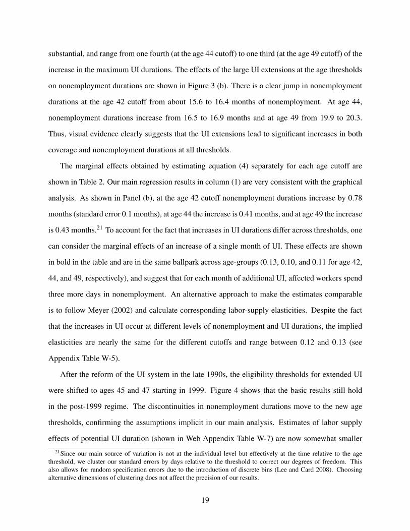
substantial, and range from one fourth (at the age 44 cutoff) to one third (at the age 49 cutoff) of the

increase in the maximum UI durations. The effects of the large UI extensions at the age thresholds

on nonemployment durations are shown in Figure 3 (b). There is a clear jump in nonemployment

durations at the age 42 cutoff from about 15.6 to 16.4 months of nonemployment. At age 44,

nonemployment durations increase from 16.5 to 16.9 months and at age 49 from 19.9 to 20.3.

Thus, visual evidence clearly suggests that the UI extensions lead to significant increases in both

coverage and nonemployment durations at all thresholds.

The marginal effects obtained by estimating equation (4) separately for each age cutoff are

shown in Table 2. Our main regression results in column (1) are very consistent with the graphical

analysis. As shown in Panel (b), at the age 42 cutoff nonemployment durations increase by 0.78

months (standard error 0.1 months), at age 44 the increase is 0.41 months, and at age 49 the increase

is 0.43 months.21 To account for the fact that increases in UI durations differ across thresholds, one

can consider the marginal effects of an increase of a single month of UI. These effects are shown

in bold in the table and are in the same ballpark across age-groups (0.13, 0.10, and 0.11 for age 42,

44, and 49, respectively), and suggest that for each month of additional UI, affected workers spend

three more days in nonemployment. An alternative approach to make the estimates comparable

is to follow Meyer (2002) and calculate corresponding labor-supply elasticities. Despite the fact

that the increases in UI occur at different levels of nonemployment and UI durations, the implied

elasticities are nearly the same for the different cutoffs and range between 0.12 and 0.13 (see

Appendix Table W-5).

After the reform of the UI system in the late 1990s, the eligibility thresholds for extended UI

were shifted to ages 45 and 47 starting in 1999. Figure 4 shows that the basic results still hold

in the post-1999 regime. The discontinuities in nonemployment durations move to the new age

thresholds, confirming the assumptions implicit in our main analysis. Estimates of labor supply

effects of potential UI duration (shown in Web Appendix Table W-7) are now somewhat smaller

21Since our main source of variation is not at the individual level but effectively at the time relative to the agethreshold, we cluster our standard errors by days relative to the threshold to correct our degrees of freedom. Thisalso allows for random specification errors due to the introduction of discrete bins (Lee and Card 2008). Choosingalternative dimensions of clustering does not affect the precision of our results.

19

than our main findings, but of the same order of magnitude and still similar across age-groups.

This reduction may partly be due to stricter monitoring of job search behavior and penalties for not

accepting suitable jobs in the new regime. When we investigate the cyclical variation of the effects

of UI in the next section we will control for this slight shift in the level of the effects.22

Our findings imply that extensions in potential UI durations lead to a significant rise in the

duration of nonemployment. They also suggest that actual UI durations respond more strongly

than nonemployment durations. For each month of potential additional UI benefits, Table 2 implies

on average individuals stay 9 to 12 days longer in UI, but only 3 days longer in nonemployment.

This means a significant fraction of workers stay in nonemployment at benefit exhaustion and

are thus directly benefiting from an extension of UI durations. For example, about 28 percent

of unemployed individuals with 12 months of potential durations exhaust their UI benefits (Web

Appendix Figures W-3). An analysis of the hazard function reveals that among exhaustees only 8

percent return to employment, while the majority enters nonemployment (Card, Chetty, and Weber

2007b).

An analysis of the hazard function also shows that the nonemployment effect we find is not

purely due to an outward shift of the spike at the benefit exhaustion point. Figure 5 displays non-

parametric regression discontinuity estimates of the survivor function (Panel a) and the hazard of

exiting nonemployment (Panel b) by duration for individuals with 12 and 18 months of UI benefits.

Panel (a) of Figure 5 illustrates how the labor supply effects are related to behavior throughout the

nonemployment spell. Integrating over the area between the two survivor functions yields the total

increase in nonemployment durations associated with the increase in the potential UI durations.

The area between the two survivor functions from month 0 to month 18 represents the increase in

actual UI durations that is due to the shift in the survivor functions, which - rescaled to marginal

changes - corresponds to dBdP

∣∣2 in the theory section. The area between months 12 and 18 under the

22 From Figure 4 it is also apparent that the duration of the average unemployment spell decreased for each age.Besides being a result from stricter monitoring, this might also be driven by an increasing incidence of temporarylow-wage jobs over this time period. Yet, the coefficient on the dummy for the post-1999 period in our regressionmodel of the annual effects of UI extensions in Section 4.2 is not statistically significant. Appendix Figure W-2 alsoshows a more visible increase in the density in the two age weeks at the two age cutoff points. Yet, the same argumentsas in Section 3.4 apply.

20

lower survivor function, represents the additional UI coverage provided when individuals do not

adjust their search behavior, which - again rescaled to marginal changes - corresponds to dBdP

∣∣1 in

the theory section.23

To better display changes in the survivor functions, Panel (b) of Figure 5. Consistent with pre-

vious studies (e.g., Meyer 2002), in Panel (b) there are clear spikes in the hazard rate at the benefit

exhaustion points for the two respective groups. However, there are also clear and statistically

significant differences well before the exhaustion point, indicating that when eligible for longer

durations, unemployed individuals adjust their search behavior a long time before running out of

UI (e.g., Card, Chetty, and Weber 2007a). These findings imply that our main effects reported in

Table 2 are averages of behavioral responses along the entire duration distribution.24

To benchmark the potential bias from sorting of individuals at the age thresholds we computed

upper and lower bounds for the employment effects using the method described in Section 3.4.

The bounds are relatively narrow, with both the lower and upper bounds being clearly statistically

significantly different from zero. For the rescaled marginal effect of actual UI durations at the

age 42 threshold, the lower bound is estimated as 0.29 while the upper bound is 0.32. For the

nonemployment effects the bounds are 0.095 and 0.17 respectively - well within the overall range

of our estimates in Table 2. Given that the economic incentives to wait are clearly stronger for

individuals with longer nonemployment duration, the true effect most likely lies between the main

estimate and the lower bound. The bounds for the other age thresholds are similar and are reported

in the Web Appendix (Table W-4).

Restriction on Labor Force Participation. To examine whether our main findings are affected

23In practice the nonemployment and UI survivor functions diverge, since individuals leave the UI system withouttaking up employment even before their benefits expire. In the Web Appendix we show the survivor functions sepa-rately (Figure W-5) and explain how we can compute the components of the welfare formula dB

dP

∣∣1 and dB

dP

∣∣2 in this

case (Figure W-6). When we analyze the cyclical variation of the two components in Section 4.2, we compute themusing the actual UI survivor functions.

24A more detailed discussion of the methodology can be found in the Web Appendix (Section 2.1). Regressiondiscontinuity estimates along different points of the duration distribution and for the other age cutoffs are shown in theWeb Appendix Table W-9. The table shows significantly negative effects on the hazard prior to the exhaustion point ofthe control group. These effects are present in the first twelve months even when potential durations increase from 22to 26 months, suggesting that individuals are forward looking over a long horizon. After the exhaustion point of thecontrol group, the difference reverses, with the hazard of the higher eligibility group exhibiting a significant increaseat the new point of exhaustion.

21

by our focus on stable workers we replicated our main RD estimates without any restriction on

labor force attachment before UI receipt. According to the law, for the full sample potential UI

durations vary between 2 and 6 months at the age thresholds, depending on the employment history.

The RD estimates for the unrestricted sample, shown in the last columns of Table 3, are smaller

than for the main sample for the durations of both UI receipt and nonemployment. Since the

underlying average changes in potential UI durations at the thresholds are also smaller, this is

consistent with the underlying true marginal effects being similar. As explained in Section 3 we

cannot calculate a rescaled marginal effect for a single month of UI extension for this group. In

order to obtain a measure comparable across samples, using the estimates in Table 2 and 3 we can

normalize our estimates of the effect of UI extensions on nonemployment duration by dividing by

the effect on actual UI duration. As discussed in Section 2, this ratio is effectively an instrumental

variables estimator of the effect of UI duration on nonemployment. This ratio is quite similar for

our main sample and the fully unrestricted sample.

Discussion. Our results are consistent with the theoretical model we discussed in Section 2.

The model predicts that a rise in the potential duration of UI benefits leads individuals to lower their

search effort (st). Consistent with our finding in Table 2, this implies a rise in the average duration

of nonemployment. Also consistent with our results, the reduction in search intensity predicts a

lower hazard of leaving unemployment for all nonemployment durations before benefit exhaustion.

Our finding that the mean duration of UI receipt increases more strongly than the nonemployment

duration implies that the increase in UI coverage is only partly due to a behavioral response. An

important part of increased coverage is due to individuals continuing to receive UI benefits, who

would otherwise have exhausted benefits while remaining in nonemployment. Our model provides

a framework for the interpretation of the effects of UI extensions on nonemployment and benefit

duration, and its implications are taken up again in Section 4.2 and the Conclusion. Finally, con-

sistent with our model, in separate work we do not find an effect of UI extensions on wages, other

measures of job quality, or long-term employment.

The labor supply responses we find are consistent with the results from previous studies in

22

Germany, Austria, and, with some qualification, the United States. Hunt (1995) evaluates the

reforms in the German UI system over the period 1983 to 1988 using a difference-in-difference

approach between age-groups over time. Hunt (1995) finds that her estimated effect on the haz-

ard rate is slightly smaller than the effect in Moffitt (1985), who reports a marginal effect of 0.16

weeks per additional week of potential UI benefits. This implies the estimates are quite comparable

despite differences in underlying samples, methodology, and measures of nonemployment dura-

tion.25 Lalive (2008) evaluates the effects of UI in Austria in a RD design that is similar to ours.

He finds that an increase of benefit durations from 30 to 209 weeks for workers age 50 increases

unemployment durations for men from 13 to 28 weeks. This implies an increase in 0.09 months

of nonemployment for each additional month of UI duration. In a different context, Card, Chetty,

and Weber (2007a) analyze increases in benefit durations in the Austrian UI system using a similar

RD design as ours but with smaller increases in potential UI durations. Their estimates point to

similarly modest labor supply effects of potential UI durations.

The marginal effects of an additional month of potential UI benefits implied by our estimates

are also in a similar range of related studies based on data from the United States. Our main

estimates of a marginal effects of around 0.1 - 0.13 are at the lower bound of United States estimates

of the effect of UI durations on labor supply surveyed in Meyer (2002). The most comparable

study to ours (Card and Levine 2000) finds similarly modest effects of exogenous extensions in

UI benefits. Other studies tend to find somewhat larger estimates (e.g., Meyer 1990, Katz and

Meyer 1990). To what extent these differences could be explained by the German institutional

environment will be discussed further in Section 5.2.25Since Hunt’s approach averages over different potential UI durations, a direct comparison with our estimates via

marginal effects or elasticities is difficult. Another paper analyzing the age-thresholds of the German UI system usingdifference-in-differences, Fitzenberger and Wilke (2010), focuses on age groups older than 50, which we excludedfrom our analysis. Note that with flexible controls for age, in our case difference-in-difference estimates would beequal to RD estimates, hence we do not pursue a direct comparison between these approaches. Caliendo, Tatsiramos,and Uhlendorf (2009) use similar data as we do from 2001-2007 to study the effect of UI extensions on job quality,but focus on individuals close to benefit exhaustion at one age threshold.

23

4.2 Variation of Labor Supply Effects with the Business Cycle

A key advantage of the institutional setting in Germany is that it provides quasi-experimental in-

creases in potential UI duration that do not vary with the business cycle. This allows us to study

variation in the effects of UI over the business cycle while holding constant potentially confound-

ing conditions in the labor market. Using the large samples in our data we replicated our regression

discontinuity estimates for our multiple age thresholds for each year and major industry, and ex-

amined whether the resulting labor supply effects and benefit durations varied systematically with

the business cycle. To do so, we could have in principle regressed the marginal effects on business

cycle indicators for the entire period during which individuals choose their search intensity, includ-

ing at the moment of benefit exhaustion. Due to high inter-temporal correlations of unemployment

rates this is unfeasible. Instead, we include a single indicator of the state of the business cycle

in our regressions. After some experimentation, as further discussed below, we have settled on a

common subset of measures capturing the current state of the labor market and the rate of new

inflows in the year of the start of a worker’s UI spell.26

Overall, the findings from this exercise suggest that the nonemployment effects of potential

UI durations are quite stable over the business cycle. At best, some of our results suggest a weak

decline in the effect of extended UI on nonemployment in recessions. In contrast, we find that the

effect of UI extensions on benefit duration, and thus the additional coverage provided, increases

significantly in recessions, mainly driven by a rise in the exhaustion rate. As a result, we show that

the nonemployment response to actual UI durations is clearly countercyclical.

The first panel of Figure 6 plots the rescaled marginal effects of a one-month increase in po-

tential UI on nonemployment duration over time. The estimates are obtained by replicating our

regression discontinuity estimates separately for each calendar year for the threshold at age 42

26As a helpful referee has pointed out, another justification for this ’reduced-form’ approach is that from the policymaker’s point of view, what matters is to optimally predict the exhaustion rate and nonemployment effect based on thecurrent state (and predicted evolution) of the economy, not to estimate the full underlying behavioral relationship. Notethat given the timing and duration of UI spells in our sample, measures of future levels and changes in unemploymentrates would also capture well the economic environment during which workers make choices. However, at the behestof the referee, we moved these results to the Web Appendix, and only include variables that are available to the policymaker in the current year.

24

(and age 45, after the 1999 reform), which yields the most precise estimates for the effects. The

unemployment rate shows how the German economy has gone through large economic swings

during our sample period, such as the dramatic boom-bust period after unification, plus an ensuing

protracted slump. Yet, while there is some variation of the estimated marginal effect over time,

from the figure there appears to be no clear systematic variation with the business cycle. In the first

panel of Figure 7 we investigate this further by plotting the marginal effect for all ages against the

change in the unemployment rate from t-1 to t, where t is the year in which the UI spell starts. As

discussed below, the change captures the flow of newly unemployed, and is an alternative measure

of the state of the labor market. There is a slight negative correlation, but overall the marginal

effect appears to be quite stable over the business cycle.

The findings from Figure 7 (a) are extended and confirmed in column (2) of Table 4. The first

four rows of the table show results from regressing the rescaled marginal effects obtained from sep-

arate RD estimates for each year and age group on different indicators of the change in economic

conditions. The first row shows that when we use a standard measure of the state of the business

cycle – GDP growth – there is a positive albeit not statistically significant correlation between the

labor-suppy effect of UI extensions and the business cycle, indicating that the disincentive effect

tends to fall when the economy contracts. The second row uses the unemployment as a more direct

measure of the state of the labor market, and finds a negative effect, also implying that the labor

supply-effect declines in recessions. Although relative to the mean labor supply effect of 0.1, a rise

in the unemployment rate of two standard-deviations (column 1) would lead to a non-negligible

decline in the effect, this is not quite statistically significant at the 10% level. One concern with

using the level of the unemployment rate is that its variation may be partly driven by the stock

of long-term unemployed and thus represent labor market conditions facing newly unemployed

workers only imperfectly. Hence, the next two rows shows two measures of the inflow rate into

unemployment. Row 3 shows the findings when we use the change in the unemployment rate as

main independent variable, whereas row 4 shows findings from using the annual mass-layoff rate

at the establishment level as calculated from our data. Again the results indicate a negative rela-

25

tionship between the state of the labor market and the effect of UI extensions on nonemployment

duration of somewhat smaller size than the unemployment rate, but the coefficients are imprecisely

estimated.

One concern with this estimates might be that they are purely based on the time-series variation

in economic conditions shown in Figure 6 (a). Hence, in the final two rows we show changes in

labor supply elasticities for workers losing their jobs in broad industries with high or low rates of

job destruction or with high or low average wage losses in their two-digit industry (as indicated

by quintiles of average industry wage loss). The job destruction rate at the industry level provides

a measure of the inflow rate. The average wage loss can be used as a proxy for the amount of

specific skill a laid-off worker is likely to lose. This is interesting because the theory predicts

unemployed workers facing higher wage losses should respond more strongly to benefit extensions.

When working at the industry level we control changes in overall labor demand by introducing

year fixed effects. The results suggest there is little significant difference in the effect of UI on

nonemployment with our measures of industry-specific economic conditions.

Figure 6 (b), Figure 7 (b) and Table 4 replicate the same analysis for the effect of potential

duration of UI benefits on the actual duration of UI benefits. Contrary to our finding for the

effect of UI extensions on nonemployment durations, it now appears that the effect on actual UI

durations is significantly countercyclical. The lower panel of Figure 6 clearly shows how there

is a substantial positive relationship between the effect of UI extensions and benefit duration and

the lead in unemployment rates. As we will see below, this correlation is driven by the cyclicality

in the UI exhaustion rate. Given potential benefit durations in our sample, it is the state of the

labor market in years t+1 or t+2 that matters. The lower panel of Figure 7 shows that there is a

positive correlation between the change in the unemployment rate, capturing a rise in the inflow

to unemployment, and actual UI benefit duration. This is not surprising, since given a high auto-

correlation of unemployment rates and relatively long unemployment durations in Germany there

is a strong correlation between current inflows and the future level unemployment.

These graphical findings are confirmed in Table 4, where we assess the correlation of the re-

26

sponse in UI duration to benefit extensions with the same range of alternative measures of the

business cycle as we did for the nonemployment effect. The table shows that the effect of UI

extensions on benefit duration tends to increase in recessions. The effect correlates strongly with

the change in unemployment rates, the mass-layoff rate, or our industry-specific measures of labor

market conditions. For these measures, a rise of two-standard deviations lead to increases in the

marginal effect of about 25-30 percent relative to the mean. While GDP growth has a smaller,

insignificant effect, the effect of the level of the unemployment rate is of the wrong sign. Given

the evidence in Figure 6 (b), it is likely that the reason is that the unemployment rate when en-

tering unemployment correlates only weakly with the labor market conditions at UI exhaustion.

That the cyclicality of the UI exhaustion rate is a key driver of the cyclicality in the response of

actual benefit durations to UI extensions is shown explicitly in two remaining columns of Table 4.

Column 5 shows how the exhaustion rate is strongly procyclical for the measures in rows 3 to 6,

while column 6 shows that the increase in benefit duration prior to the exhaustion point, which is

driven by a shift in the survivor function, varies little with the cycle. As further discussed below,

this has potentially important implications for the welfare impact of UI extensions.

In the theory section we showed that the ratio of the nonemployment effect and the effect on

effect on actual benefit durations, dD/dB = dDdP

/ dBdP represents a summary measure of the disin-

centive effect that is relevant from a welfare perspective. The ratio, which captures the effect of

an actual increase in UI benefit duration on nonemployment duration, effectively normalizes for

changes in the intensity of treatment over the business cycle, since dBdP rises with the exhaustion rate

and hence with the number of people potentially affected by UI benefit extensions. The cyclical

variation of the so ’normalized’ disincentive effect is shown in Column (4) of Table 4. Unlike

the marginal effect dDdP this normalized disincentive effect is strongly countercyclical. Out of the

6 regressions, it is statistically significantly correlated with 5 measures of the business cycle. The

effect of a worsening of our measures by two-standard deviations is substantial and in the same

range for all measures but for the level of the unemployment rate, for which it is a bit smaller.

However, the effect of the level of the unemployment rate is now of the right sign.

27

Our main findings in Table 4 are very robust and in some cases stronger when we consider

important extensions in Table 5. To save space, Table 5 only shows the results for using the level

and change of the unemployment rate as our measures of cyclical conditions, and relegate the

estimates for additional measures to the Web Appendix (Table W-16). The first column of the

table replicates our main findings in Table 4 for a bandwidth of one year. In several instances, the

negative correlation of the marginal nonemployment effect and the ratio dDdP

/ dBdP is now stronger

and statistically significant. It is worth noting that the nonemployment elasticity (shown for our

main estimates in column (7) of Table 4), is now also significantly negatively correlated with the

business cycle.27

The second column shows the lower bound discussed in Section 3.4, where we reallocate the

excess mass of spells from the right to the left of the cutoff, and assign them the highest nonem-

ployment durations in the sample. This would be the right estimator if all these workers had

purposefully waited to gain access to longer benefits because they have the longest spells. Similar

to the findings in column (1), these results tend to show somewhat stronger counter-cyclicality of

the nonemployment effect and hence the ratio. To further account for potential selection due to

voluntary quitters, who are required by law to wait 85 days before becoming eligible for UI, and

also address the issue discussed in Section 3 that voluntary quitters may have a stronger incen-

tive to wait to gain access to benefits above the threshold, column (3) drops anyone waiting more

than two weeks before taking up UI benefits. The estimates are very similar to the main results in

Table 4.

If characteristics of UI recipients change over time or vary with the business cycle and treatment

effects vary across groups, another concern could be that such changes in composition could offset

potential cyclical variation in labor supply effects of UI. We examined this possibility, and found

it not to affect our result. We analyzed cyclical variation in two summary indices of observable

characteristics in our data, the predicted propensity to receive unemployment assistance (UA) and

27This suggests that the elasticity is another possible way to rescale the marginal effect by the intensity of treatmentas suggested in Section 2. However, the counter cyclicality is considerably weaker than that of the ratio dD/dB,because the average duration of nonemployment is also determined by other factors than treatment intensity.

28

the predicted post-UI wage. Overall, relative to the mean we found at best very small variations

in observable characteristics with the business cycle. To nevertheless make sure these changes

do not affect our findings, we used the standard re-weighting procedure to hold distribution of

characteristics constant across years. This is shown in column (4) of Table 5 and confirms that

our findings are very robust to changes in characteristics of UI recipients over time or the business

cycle.

Finally, to address the concern that our findings are limited to our main sample of workers

with high employment attachment, columns (5) and (6) of Table 5 show results when we include

all workers irrespective of labor market experience. As discussed in Section 3.2, for this sample

we cannot calculate rescaled marginal effects. However, the ratio of marginal effects has the same

interpretation as for the restricted sample. The third panel of the table shows the results when using

two and one year bandwidths to generate the estimates. The point estimates for the measures in

the table are somewhat smaller compared to our more restricted sample when we use a bandwidth

of two years (though identical and precisely estimated when we use the mass-layoff rate, as shown

in Web Appendix Table W-16) and quite similar and more precisely estimated when we use a

bandwidth of two years. Hence, our main results holds for a very broad sample of unemployed

individuals and are not restricted to high-attachment workers.

Overall, we conclude that our main estimates for the effect of UI durations on labor supply

do not vary strongly with the business cycle, but that the exhaustion rate, and with it the effect on

benefit duration, is countercyclical. In several specifications we find a small decrease in the labor

supply effect of UI durations in recessions, but in most instances the correlation is not statistically

significant from zero. However, these findings show that the effect of a rise of actual benefit

duration on nonemployment duration, which effectively normalizes for the increase in the number

of workers ’at risk’ of being affected by extended UI durations in recessions, has a clear and

precisely estimated countercyclical pattern.

Discussion. To see how our empirical results relate to the theory we outlined in Section 2,

it is useful to consider a slightly modified version of our main welfare formula. To express our

29

welfare formula fully in terms of statistics that can potentially be measured empirically we follow

Chetty (2008) and normalize equation (2) by the expected marginal utility of employed workers.

The resulting rescaled welfare gain is approximately equal to

dW0

dP=

dBdP

b[−∂sP/∂aP

∂sP/∂wP

]− dD

dPbΩ (5)

where the new term in the first bracket is the ratio of the ’liquidity’ effect (∂sP/∂aP) and the ’sub-

stitution’ effect (−∂sP/∂wP) of a UI extension for workers exhausting UI benefits.28 If available,

using appropriate empirical measures of the income and substitution effects one can assess whether

at a given duration of UI benefits, an extension would be welfare improving. Changes in the wel-

fare effect of extensions in UI benefit durations over the business cycle arise from variation in three

main components, dBdP (or effectively the exhaustion rate), the nonemployment effect (dD

dP ), and the

relative strength of the liquidity vs. substitution effect of UI benefits.

As mentioned in Section 2, to relate our empirical findings to the theoretical welfare formula

it is important to realize that what is relevant for the formula is the effective exit rate from nonem-

ployment, and hence what we labeled a general-equilibrium or macro effect in Section 2. Our

empirical estimates hold variation in the macroeconomic environment constant and thus obtain the

partial-equilibrium or micro effect. Changes arising from the exhaustion rate (which is a mechani-

cal effect) suggest that the number of beneficiaries from UI extensions are rising in recessions. Yet,

as further discussed in our conclusion in the Conclusion, whether our empirical estimates imply

that the effective nonemployment effect of UI durations, and hence the efficiency cost from UI

extensions, also declines in recessions requires further information.

28We have that dW0/dP ≡ (dW0/dP)/E0,T−1v′(cet ). The result in our second formula holds as long as on average

unemployment durations are short relative to life-time employment, such that the marginal utility after unemploymentis similar to the expected marginal utility at employment in t = 0. For details see the Web Appendix Section 3.

30

5 Robustness

Our main results are very robust to many alternative specifications, which are briefly summarized

in this section. Additional details are relegated to our Web Appendix.

5.1 Robustness Analysis

Choice of Bandwidth. We investigated whether the choice of the bandwidth of the RD estimator

affects our conclusions (Table 2). Using a bandwidth of 2 years, the point estimates from the RD

regressions are very similar to what is implied by the graphical analysis. For smaller bandwidths

coefficients are very stable for the effects on UI durations, even with bandwidths as small as 0.5 or

0.2 years. For the nonemployment durations the estimates are in the same ballpark across different

bandwidths, but somewhat larger for tighter bandwidths. Investigating figures with different band-

widths revealed that this is due to under-smoothing for very small bandwidths, so that we have

most confidence in estimates with 2 year bandwidths. As discussed in Section 4.2, our estimates

in column (1) of Table 5 also imply that our results regarding cyclicality are robust to choosing a

narrower bandwidth.29

Measure of Nonemployment. We also find that the increase in nonemployment durations is

mainly due to workers taking longer until returning to a job, not due to individuals staying out of

employment forever. In order to investigate this Table 3 column (2) shows the probability of ever

returning to registered employment. There is a slight drop of one percent relative to the mean of

0.77 (Appendix Table A-1) at the age 42 cutoff, and the effect is even smaller for the other two age

thresholds. Even though it is statistically significant, the slight decline in the fraction of workers

ever returning to work accounts for a very small increase in overall nonemployment durations.

Similarly we investigated whether our estimates are affected by the choice of our nonemployment

duration measure. For example, as an alternative we replicated all of our findings with time-to-

29It should be noted that 2 years is a very narrow bandwidth in comparison to other papers with a similar RD design.For example, Card, Chetty, and Weber (2007) use a polynomial in age without a bandwidth; Lalive (2008) shows aspecification with a two-year bandwidth, but his preferred specifications use polynomials in age without bandwidth;Lemieux and Milligan (2008) use bandwidths of six years

31

next-job for workers who return to employment. Consistent with the result that the incidence of

censoring does not vary strongly at the eligibility thresholds, our results are largely unaffected by

this choice.30

Differences by Subgroups. To further examine the robustness of our main estimates, Table 6

shows our regression discontinuity estimates for several subgroups. While the table displays some

expected differences in the labor supply response to UI extensions, overall the labor supply effects

are remarkably robust throughout the population. In particular, it does not appear that our findings

are driven by any particular sub-group in our sample. The labor supply effects are slightly larger

but not significantly different for highly educated and high tenure workers, and larger and signif-

icantly different for women. Together with the similarities across age-groups, the point estimates

in Table 6 imply a common labor supply effect of an additional month of UI benefits in the range

from 0.1 to 0.18.

Robustness of Differences over Cycle. We estimated many additional specifications to those

reported in Section 4.2 to further investigate the robustness of the findings regarding the cyclical

variation of the effect of UI extensions. For example, dropping UI spells from East Germany

from our sample, or excluding temporary lay-offs (workers who return to their old employer),

did not affect the results reported in Table 4. One potential concern with our main estimates

in Table 4 is that they mask differential effects over the cycle in different parts of the duration

distribution. We compared shifts in the entire hazard function across boom and bust periods in

the Web Appendix (Figure W-4), and did not find this to be the case. We also tried several ways

to further raise precision of our estimates. For example, when we split our sample by worsening

and improving labor market conditions, the labor supply effect seems to be somewhat lower in

worsening times (Web Appendix Table W-11). Alternatively we estimated a cox-proportional

hazard model in the spirit of Meyer (1990) and find a slight decline in the predicted labor supply

elasticities when unemployment is increasing (Web Appendix Table W-12). We also estimated a

30Web Appendix Table W-5 provides a summary of the various steps in the sensitivity analysis, such as usingdifferent censoring rules. See Card, Chetty, and Weber (2007b) for further discussion of alternative measures ofunemployment spells.

32

linear and log-linear models that pool the effect of UI extensions across our different age-thresholds

while flexibly controlling for age (Web Appendix Table W-13). Again, the changes over time we

find are relatively small, with at best weakly negative coefficients on the interaction of potential UI

duration and business cycle indicators.

5.2 The Role of Unemployment Assistance

In this section we discuss to what extent our results may be affected by relatively generous UI

replacement rates and by the presence of unemployment assistance (UA). On the one hand, high

replacement rates implies that our relatively modest effects would over-predict the effect relative to

a system with lower replacement rates.31 On the other hand, the presence of UA after exhaustion

of UI benefits should lead to smaller effects, since the strength of the disincentive effect of UI

depends on the net change in replacement rates at exhaustion. In this context, the fact that women

have only somewhat higher responses than men is interesting, since as discussed in Section 3 for

the typical married woman with a working husband (which is a majority in our age-range) the

benefit provided by UA after exhaustion of UI benefits is close to zero. This suggests that presence

of UA per se may not strongly affect our estimates. To learn more about the potential role of

extended UA in explaining our findings, we replicated our main regression discontinuity estimates

for individuals with high and low propensities to receive UA. If our main estimates were mainly

driven by individuals entering UA after exhausting benefits, we should see significant disparities

here. The last rows of Table 6 shows that this is not the case. About 10-15% of UI beneficiaries and

50% of exhaustees receive UA. For each UI recipient in our sample we predicted the propensity to

receive UA based on education, demographic characteristics, and their earnings histories.32 The

31The presence of a cap on earnings implies the average replacement rate is likely to be somewhat lower than thenominal rate, but still more generous than, say, in the United States, where more stringent maximum weekly benefitsimply that nominal replacement rates of about 50 percent turn to average replacement rates of close to 40 percent.Since UI benefits in the United States are subject to income taxes, but usually taxed at a lower rate than earnings, thisis likely to somewhat understate the effective replacement rate.

32The corresponding linear probability model is shown in the Web Appendix Table W-10, and suggests our spec-ification has a good fit. The average predicted value for the probability of take up of UA at exhaustion for the fullsample is 0.54, which can be thought of as an estimate of the fraction of UI recipients who are potentially eligiblefor UA. Note that given the determination of UA benefits, ideally we would have had also access to wealth, maritalstatus, and spousal earnings to make this prediction. Wealth closely correlates with education and earnings histories.

33

rescaled marginal effect for individuals whose propensity is above and below 0.5 is 0.1 and 0.18,

respectively (the proportion of workers with with low propensity is about 30%). If we include an

interaction with the individual propensity and extrapolate linearly, for individuals with propensity

of receiving UA close to 80% the rescaled marginal effect is below 0.05. Yet, even for those whose

propensity is 20% it is 0.25, well within the overall magnitude of our main findings. Thus, we

conclude that while individuals seem to respond to the incentives inherent in UA, and hence the

presence of UA may lead to somewhat smaller overall estimates, it is unlikely to be the main source

behind the labor supply effects we find.

6 Conclusion

In this paper, we estimate how the effect of extensions in the duration of unemployment insurance

benefits (UI) on nonemployment and benefit duration varies over the business cycle. To do so, we

use the universe of unemployment spells in Germany over 20 years, where differences in potential

UI durations by age allow for the implementation of a regression discontinuity design. Since

the age discontinuities do not vary with economic conditions, they provide multiple valid quasi-

experiments throughout the business cycle, allowing us to avoid endogeneity problems arising

when parameters of UI respond to the business cycle. Our findings indicate a modest effect of

extensions in UI durations on nonemployment durations of comparable magnitude to what has

been found before. This effect is quite stable in different economic environments. At best some

specifications point to slightly smaller nonemployment effects during recessions. On the other

hand we find that the additional coverage provided by UI extensions is strongly increasing in

recessions, mainly due to a sharp increase of the fraction unemployed who otherwise would have

exhausted their UI benefits. As a result, the ratio of the effect of UI extensions on nonemployment

and benefit durations – which captures the reduction in nonemployment duration for a given rise

in UI durations and hence is a measure of the disincentive effect that controls for changes in the

take-up of UI benefits over the business cycle – is significantly counter-cyclical.

Unfortunately, we currently do not have access to marital status, and neither wealth or spousal earnings are in our data.

34

To help interpret these findings, we show in a search model with liquidity constraints that

the welfare effect of UI extensions is the sum of two components: the benefit provided by the

additional coverage for individuals who otherwise would have exhausted UI benefits, and the cost

due to the disincentive effect of UI, which leads to an increased tax burden for the employed. This

result clarifies that the optimal duration of UI benefits does not only depend on the the exhaustion

rate (Corson and Nicholson 1982) or on the nonemployment effect (Moffitt 1985) alone, but on

both. We also show that the welfare gain from UI extensions can be expressed as a function of the

ratio of the effect of UI extensions on nonemployment and benefit durations. As in prior related

literature on UI benefit levels, a decline in this ratio and hence a reduction in the effective moral

hazard of UI extensions ceteris paribus raises the optimal duration of UI benefits.

The welfare formula that we derive from our model, together with our findings of weakly

declining nonemployment effects and strongly countercyclical exhaustion rates implies that the

optimal duration of UI benefits should rise in recessions only under two conditions. First, if the

marginal utility of the unemployed is constant or increasing during recessions. Second, if the

cyclical movement of the partial-equilibrium effects identified in this paper provide a good ap-

proximation of the cyclicality of general equilibrium effects. In this case our results also suggest

that countries with constant UI durations over the cycle, such as Germany and most other European

countries, may raise welfare by moving to a system with counter-cyclical potential UI durations.

Whether these two important conditions hold are important empirical questions beyond the

scope of this paper. For example, a reduction in the ability to self-insure through a decline in

wealth in recessions would lead to a rise in the marginal utility of consumption of the unemployed

and thus in the value of insurance. Existing evidence from the United States suggests that this

"liquidity" effect does not appear to vary significantly with the business cycle. A bigger challenge,

both theoretically as well as empirically, is that UI extensions may affect nonemployment dura-

tions by affecting the overall state of the labor market. The importance of such general equilibrium

channels can not be estimated in our regression discontinuity design, which by construction com-

pares individuals with different potential UI durations in the same labor market. To what extent the

35

general equilibrium or macro effect of UI extensions is smaller or greater than the partial equilib-

rium or micro effect we measure depends on a range of factors lying outside the scope of our model

and our empirical analysis. In the presence of search externalities; if there is incomplete take up

of UI benefits; if UI extensions raise aggregate demand; or if recessions involve job rationing (as

in the model of Landais, Michaillat, and Saez 2010), then our partial equilibrium effects represent

a lower bound of the efficiency cost of UI. If on the other hand recessions involve the need for

reallocation (e.g., as in Sargent and Ljungvist 1998) or if UI extensions reduce the incentives to

create vacancies, then our estimates may represent upper bounds.

An advantage of the welfare formula we derive is that it can be fully expressed in terms of

’sufficient statistics’ that can be estimated in the data (Chetty 2008). Thus, to implement the wel-

fare formula and calculate the welfare gain from an extension in UI durations in recessions, future

research should obtain estimates of variation in both the liquidity effect of UI extensions and the

general equilibrium effect of UI extensions on nonemployment durations. Although the fact that

Card, Chetty, and Weber (2007a) report similar labor supply effects for broader age groups for

Austria with a similar RD design as ours is reassuring, a further useful extension of our work

would be to obtain similar estimates of the effect of UI extensions on nonemployment and benefit

durations over the business cycle for younger workers. Our research design also does not allow

us to directly assess the labor supply effect of indefinite unemployment assistance (UA) available

in Germany after UI is exhausted. Our results indicate that variation in the likelihood unemploy-

ment assistance has predictable effects, but assessing the labor supply effect of UA directly is an

important avenue for future research.

36

References

[1] T. ANDERSEN AND M. SVARER, State Dependent Unemployment Benefits, Journal of Riskand Insurance, 78 (2010), pp. 325–344.

[2] J. ANGRIST AND G. IMBENS, Two-Stage Least Squares Estimation of Average Causal Ef-fects in Models with Variable Treatment Intensity, Journal of the American Statistical Asso-ciation, 90 (1995), pp. 431–442.

[3] M. ARNTZ, S. LO, AND R. WILKE, Bounds Analysis of Competing Risks: A NonparametricEvaluation of the Effect of Unemployment Benefits on Imigration in Germany, ZEW Discus-sion Papers, 07-049 (2007).

[4] M. BAILY, Some Aspects of Optimal Unemployment Insurance, Journal of Public Economics,10 (1978), pp. 379–402.

[5] S. BENDER, A. HAAS, AND C. KLOSE, IAB Employment Subsample 1975-1995 Opportuni-ties for Analysis Provided by the Anonymised Subsample, IZA Discussion Paper, 117 (2000).

[6] M. BROWNING AND T. CROSSLEY, Unemployment insurance benefit levels and consump-tion changes, Journal of Public Economics, 80 (2001), pp. 1–23.

[7] M. CALIENDO, K. TATSIRAMOS, AND A. UHLENDORFF, Benefit duration, unemploymentduration and job match quality: A regression-discontinuity approach, IZA Discussion Paper,4670 (2009).

[8] D. CARD, R. CHETTY, AND A. WEBER, Cash-On-Hand and Competing Models of Intertem-poral Behavior: New Evidence from the Labor Market, Quarterly Journal of Economics, 122(2007a), pp. 1511–1560.

[9] , The spike at benefit exhaustion: Leaving the unemployment system or starting a newjob?, American Economic Review Papers and Proceedings, 97 (2007b), pp. 113–118.

[10] D. CARD AND P. LEVINE, Extended benefits and the duration of UI spells: evidence from theNew Jersey extended benefit program, Journal of Public Economics, 78 (2000), pp. 107–138.

[11] R. CHETTY, Moral hazard versus liquidity and optimal unemployment insurance, Journal ofpolitical Economy, 116 (2008), pp. 173–234.

[12] CONGRESSIONAL BUDGET OFFICE, Family Income of Unemployment Insurance Recipients,Policy Brief, March (2004).

[13] W. CORSON AND W. NICHOLSON, The Federal Supplemental Benefits Program: An Ap-praisal of Emergency Extended Unemployment Insurance Benefits, Kalamazoo, MI: W.E.Upjohn Institute for Employment Research, 1982.

[14] B. FITZENBERGER AND R. WILKE, Unemployment Durations in West Germany Before andAfter the Reform of the Unemployment Compensation System During the 1980s, GermanEconomic Review, 11 (2010), pp. 336–366.

37

[15] J. GRUBER, The consumption smoothing benefits of unemployment insurance, The AmericanEconomic Review, 87 (1997), pp. 192–205.

[16] H. HOPENHAYN AND P. NICOLINI, Optimal Unemployment Insurance, Journal of PoliticalEconomy, 105 (1997), pp. 412–438.

[17] J. HUNT, The Effect of Unemployment Compensation on Unemployment Duration in Ger-many, Journal of Labor Economics, 13 (1995), pp. 88–120.

[18] N. F. J. DINARDO AND T. LEMIEUX, Labor market institutions and the distribution ofwages, 1973-1992: A semiparametric approach, Econometrica, 64 (1997), pp. 1001–44.

[19] S. JURAJDA AND F. J. TANNERY, Unemployment durations and extended unemploymentbenefits in local labor markets, Industrial and Labor Relations Review, 56 (2003), pp. 324–348.

[20] L. KATZ AND B. D. MEYER, The Impact of Potential Duration of Unemployment Benefits onthe Duration of Unemployment Outcomes, Journal of Public Economics, (1990), pp. 45–71.

[21] M. T. KILEY, How Should Unemployment Benefits Respond to the Business Cycle?, TheB.E. Journal of Economic Analysis and Policy, (2003).

[22] K. KROFT AND M. NOTOWIDIGDO, Should unemployment insurance vary with the localunemployment rate? theory and evidence, mimeo, (2010).

[23] A. KRUEGER AND B. MEYER, Labor supply effects of social insurance, Handbook of publiceconomics, 4 (2002), pp. 2327–2392.

[24] J. LAKE, Temporary Programs to Extend Unemployment Compensation, Congressional Re-search Service Reports and Issue Briefs, 10-1 (2002).

[25] R. LALIVE, How do extended benefits affect unemployment duration? A regression disconti-nuity approach, Journal of Econometrics, 142 (2008), pp. 785–806.

[26] C. LANDAIS, P. MICHAILLAT, AND E. SAEZ, Optimal unemployment insurance over thebusiness cycle, NBER Working Paper, 16526 (2010).

[27] D. LEE AND D. CARD, Regression discontinuity inference with specification error, Journalof Econometrics, 142 (2008), pp. 655–674.

[28] D. LEE AND T. LEMIEUX, Regression discontinuity designs in economics, Journal of Eco-nomic Literature, 48 (2010), pp. 281–355.

[29] T. LEMIEUX AND K. MILLIGAN, Incentive effects of social assistance: A regression discon-tinuity approach, Journal of Econometrics, 142 (2008), pp. 807–828.

[30] R. LENTZ AND T. TRANAES, Job search and savings: Wealth effects and duration depen-dence, Journal of Labor Economics, 23 (2005), pp. 467–489.

38

[31] L. LJUNGQVIST AND T. SARGENT, The European unemployment dilemma, Journal of Po-litical Economy, 106 (1998), pp. 514–550.

[32] , Two Questions about European Unemployment, Econometrica, 76 (2008), pp. 1–29.

[33] J. MCCRARY, Manipulation of the running variable in the regression discontinuity design:A density test, Journal of Econometrics, 142 (2008), pp. 698–714.

[34] B. D. MEYER, Unemployment Duration and Unemployment Spells, Econometrica, 58(1990), pp. 757–82.

[35] , Unemployment and workers compensation programmes: rationale, design, labour sup-ply and income support, Fiscal Studies, 23 (2002), pp. 1–49.

[36] R. MOFFITT, Unemployment Insurance and the Distribution of Unemployment Spells, Jour-nal of Econometrics, 28 (1985), pp. 85–101.

[37] C. A. MYERS AND W. MACLAURIN, After Unemployment Benefits are Exhausted, Journalof Public Economics, 56 (1942), pp. 231–255.

[38] J. NEEDELS AND W. NICHOLSON, Extended Unemployment Benefits: A Review of the Lit-erature, mimeo, (2004).

[39] N. PAVONI, On Optimal Unemployment Compensation, Journal of Monetary Economics, 54(2007), pp. 1612–1630.

[40] J. M. SANCHEZ, Optimal state-contingent unemployment insurance, Economics Letters, 98(2008), pp. 348 – 357.

[41] J. F. SCHMIEDER, T. VON WACHTER, AND S. BENDER, The Long-Term Impact of Job Dis-placement in Germany During the 1982 Recession on Earnings, Income, and Employment,Columbia University, Department of Economics Discussion Paper Series, DP0910-07 (2009).

[42] R. SHIMER AND I. WERNING, Reservation Wages and Unemployment Insurance, QuarterlyJournal of Economics, 122 (2007), pp. 1145–1185.

[43] G. SOLON, Labor Supply Effects of Extended Unemployment Benefits, Journal of HumanResources, 14 (1979), pp. 247–255.

[44] T. VON WACHTER, J. SONG, AND J. MANCHESTER, Long-Term Earnings Losses due toMass-Layoffs During the 1982 Recession: An Analysis Using Longitudinal AdministrativeData from 1974 to 2004, mimeo, (2009).

[45] R. WILKE, New Estimates of the Duration and Risk of Unemployment for West-Germany,Journal of Applied Social Science Studies, 128 (2005), pp. 207–237.

39

Tables

Table 1: Regression Discontinuity Estimates of Smoothness of Predetermined Variablesaround Age Discontinuities in Potential Duration of Unemployment Insurance (UI) Ben-efits

(1) (2) (3) (4) (5) (6) (7)Years of Female Foreign Tenure Occupation Industry Wage

Education Citizen Last Job Tenure Tenure Last JobLast Job Last Job

D(age>=42) 0.027 0.0056 0.0023 -0.010 -0.038 -0.017 0.28[0.014] [0.0028]* [0.0021] [0.028] [0.036] [0.016] [0.21]

Observations 452749 452749 452749 452749 452749 452749 418667

D(age>=44) -0.0092 0.00016 -0.00088 -0.045 -0.052 -0.023 0.078[0.013] [0.0028] [0.0024] [0.029] [0.037] [0.017] [0.20]

Observations 450280 450280 450280 450280 450280 450280 413874

D(age>=49) 0.026 0.010 -0.000038 -0.0072 -0.070 -0.011 -0.12[0.014] [0.0036]** [0.0034] [0.034] [0.045] [0.021] [0.26]

Observations 329680 329680 329680 329680 329680 329680 292706

Notes: The coefficients estimate the magnitude of the change in the dependent variable at the age thresh-old. Each coefficient is estimated in a separate RD regression that controls linearly for age with differentslopes and bandwidth of two age years on each side of cutoff. Standard errors (in parentheses) are clus-tered at the day level (* P<.05, ** P<.01).The sample consists of individuals starting unemployment spells between July 1987 and March 1999, whohad worked for at least 52 months in the last 7 years without intermittent UI spell. Last job refers to thelast job prior to starting the unemployment insurance spell. Means are shown in Appendix Table A-1.

40

Table 2: Regression Discontinuity Estimates of Potential Unemployment Insurance(UI) Benefit Duration (P) on Months of Actual UI Benefit Receipt and Months ofNonemployment

(1) (2) (3) (4)Age bandwidth around age discontinuity

2 years 1 year 0.5 years 0.2 years

Panel A: Dependent Variable: Duration of UI Benefit receipt (B)

D(age>=42) 1.78 1.82 1.73 1.65[0.036]** [0.052]** [0.072]** [0.11]**

Effect of 1 add. Month of Benefits dBdP 0.30 0.30 0.29 0.28

Observations 452749 225774 112436 45301

D(age>=44) 1.04 1.16 1.13 1.24[0.047]** [0.065]** [0.092]** [0.15]**

Effect of 1 add. Month of Benefits dBdP 0.26 0.29 0.28 0.31

Observations 450280 225134 112597 45258

D(age>=49) 1.40 1.44 1.44 1.72[0.074]** [0.084]** [0.12]** [0.18]**

Effect of 1 add. Month of Benefits dBdP 0.35 0.36 0.36 0.43

Observations 329680 217942 109238 43812

Panel B: Dependent Variable: Nonemployment Duration (D)

D(age>=42) 0.78 0.92 1.04 0.79[0.086]** [0.12]** [0.17]** [0.27]**

Effect of 1 add. Month of Benefits dDdP 0.13 0.15 0.17 0.13

Observations 452749 225774 112436 45301

D(age>=44) 0.41 0.63 0.62 0.78[0.089]** [0.13]** [0.18]** [0.30]*

Effect of 1 add. Month of Benefits dDdP 0.10 0.16 0.15 0.20

Observations 450280 225134 112597 45258

D(age>=49) 0.43 0.52 0.56 0.79[0.11]** [0.13]** [0.19]** [0.29]**

Effect of 1 add. Month of Benefits dDdP 0.11 0.13 0.14 0.20

Observations 329680 217942 109238 43812

Notes: The coefficients estimate the magnitude of the change in benefit or Nonemployment du-ration at the age threshold. Each coefficient is estimated in a separate RD regression that controlslinearly for age with different slopes on each side of cutoff. Standard errors (in parentheses) areclustered at the day level (* P<.05, ** P<.01).At the age 42 discontinuity potential UI benefit durations (P) increase from 12 to 18 months,at the age 44 discontinuity from 18 to 22 months and at the age 49 discontinuity from 22 to26 months. The sample consists of individuals starting unemployment insurance spells betweenJuly 1987 and March 1999, who had worked for at least 52 months in the last 7 years withoutintermittent UI spell. For the age 49 cutoff and bandwidth 2 years column, the regression onlyincludes individuals 47 and older and younger than 50, due to the early retirement discontinuityat age 50 (see text).

41

Table 3: Regression Discontinuity Estimates of Effect Of Potential Unemployment Insur-ance (UI) Benefit Duration on Additional Employment Outcomes and Estimates Based onSample without Labor-Force Restrictions

(1) (2) (3) (4) (5) (6)Time until Ever emp. Emp. UI or UA UI Duration Nonemp DurationUI Claim again 5 years 5 years No Exp. No Exp.

later later restrictions restrictions

D(age>=42) -0.00089 -0.01 -0.0041 0.0049 0.98 0.45[0.020] [0.0022]** [0.0029] [0.0021]* [0.016]** [0.036]**

Observations 452749 452749 452749 452749 2467954 2467954

D(age>=44) 0.016 -0.0056 -0.0076 0.0051 0.46 0.21[0.021] [0.0024]* [0.0030]* [0.0023]* [0.019]** [0.036]**

Observations 450280 450280 450280 450280 2293865 2293865

D(age>=49) -0.0027 -0.0076 -0.0012 0.0047 0.76 0.40[0.025] [0.0036]* [0.0038] [0.0032] [0.032]** [0.050]**

Observations 329680 329680 329680 329680 1550099 1550099

Notes: The coefficients estimate the magnitude of the change in the dependent variable at the age thresh-old. Each coefficient is estimated in a separate regression discontinuity model that controls linearly forage with different slopes and bandwidth of two age years on each side of cutoff. Standard errors (inparentheses) are clustered at the day level (* P<.05, ** P<.01).The sample for columns (1) to (4) consists of individuals starting unemployment spells between July1987 and March 1999, who had worked for at least 52 months in the last 7 years without intermittentUI spell. The sample for columns (5) and (6) consists of all individuals starting unemployment spellsbetween July 1987 and March 1999 without restriction on employment history or UI receipt prior to thecurrent UI spell. UA refers to means tested unlimited unemployment assistance available at exhaustionof UI benefits (see text).

42

Table 4: The Correlation of Annual Regression Discontinuity Estimates of Extensions in UI Benefit Durations on Nonemployment andActual Benefit Duration with Alternative Measures of the Economic Environment

Dependent Variable (1) (2) (3) (4) (5) (6) (7)Mean & Nonemployment UI-Benefits Nonemp. Duration UI Exhaustion Rate Additional NonemploymentStandard Duration: Duration: Marg. Effect (Additional UI Beneficaries DurationDeviation Rescaled Rescaled scaled by UI Beneficiaries due only to Shift of Elasticity

Marginal Effect Marginal Effect UI-Benefits holding Survivor Survivor FunctionDuration Function constant)

Marg. EffectIndependent Variable dD

dPdBdP

dDdP /

dBdP

dBdP

∣∣∣1

dBdP

∣∣∣2

ηD,P

Dependent Variable Varies by Year and Age-Threshold

Real GDP Growth from 2.15 0.0078 -0.012 0.045 -0.011 -0.00086 0.011Year t-1 to t [1.58] [0.0065] [0.0081] [0.023]† [0.0055]† [0.0048] [0.0071]

National Unemployment Rate 9.09 -0.0099 -0.0053 -0.032 -0.00059 -0.0047 -0.011in Year t [1.64] [0.0063] [0.0084] [0.024] [0.0061] [0.0046] [0.0070]

Change in Unemployment Rate 0.13 -0.012 0.038 -0.10 0.029 0.0086 -0.019from Year t-1 to t [0.78] [0.013] [0.014]* [0.042]* [0.0093]** [0.0091] [0.014]

Fraction of Establishments with 1.31 -0.022 0.059 -0.17 0.048 0.010 -0.035Mass Layoffs in Year t [0.53] [0.020] [0.022]* [0.065]* [0.014]** [0.015] [0.022]

Dependent Variable Varies by Year and 1-digit Industry and Age-Threshold

Job Destruction Rate in 1-digit 0.090 0.52 1.39 -2.32 1.25 0.14 0.26Industry from Period t-1 to t [0.032] [0.49] [0.28]** [1.20]† [0.17]** [0.27] [0.51]

Dependent Variable Varies by Year and Quintile of Average 2-digit Industry Wage Change and Age-Threshold

Mean Change in Log Wages within -0.047 -0.033 -0.56 0.98 -0.62 0.063 0.089Quintile of 2-dig. Ind. Wage Change [0.079] [0.15] [0.093]** [0.47]* [0.047]** [0.089] [0.17]

Mean of Dep Var 0.10 0.28 0.36 0.44 -0.15 0.11

Notes: Stars indicate confidence levels: †P<.1, * P<.05, ** P<.01.Columns (2)-(7) report coeffients from a 2 step regression. In the first step the effect of Extended UI durations on nonemployment durations are estimated separately for all years andage thresholds using the regression discontinuity estimator. All RD marginal effects are computed using a 2 year bandwidth and control for linear age splines with different slopes oneach side of the cutoff. In the second step the resulting marginal effects (columns) are regressed on measures of the economic environment (rows). Each reported coefficient representsthe coefficient on those measures, given in the row names. The second step regressions also include a dummy for marginal effects measured after the 1999 reform. Standard errorsare computed to allow for a common error-component at the year level. A mass-layoff is defined as a 30A mass-layoff is defined as a 30% drop in employment over a year. The rateis calculated among all establishments with at least 50 employees in the baseline year.

43

Table 5: Alternative Specifications for the Correlation of Annual Regression Discontinuity Estimates ofExtensions in UI Benefit Durations on Nonemployment and Actual Benefit Duration with the EconomicEnvironment - Smaller Bandwidth, Reweighted, Unrestricted Sample

(1) (2) (3) (4) (5) (6)Bandwidth Lower Bound Sample Restr. Sample Full Sample: Full Sample:for RD Est. for Estimates to UI take up Reweighted to No Experience No Experience

1 Year in RD Est. within 15 Days Characteristics Restrictions Restrictionsof Job Ending of Year 2000 Bandwidth Bandwidth

2 Years 1 Year

Nonemp. Duration Marginal Effect: dDdP

National Unemployment Rate -0.019 -0.011 -0.012 -0.014 – –in Year t [0.0065]* [0.0057]† [0.0096] [0.011]

Change in Unemployment Rate -0.019 -0.022 -0.0100 -0.020 – –from Year t-1 to t [0.015] [0.011]† [0.020] [0.022]

UI-Benefit Duration Marginal Effect: dBdP

National Unemployment Rate -0.0059 -0.0044 -0.0060 -0.0049 – –in Year t [0.0093] [0.0087] [0.0092] [0.0090]

Change in Unemployment Rate 0.042 0.040 0.040 0.036 – –from Year t-1 to t [0.015]* [0.014]* [0.015]* [0.015]*

Nonemp. Duration scaled by UI-Benefit Duration Marginal Effect: dDdB = dD

dP /dBdP

National Unemployment Rate -0.059 -0.039 -0.026 -0.037 -0.00095 -0.039in Year t [0.024]* [0.026] [0.029] [0.026] [0.027] [0.027]

Change in Unemployment Rate -0.13 -0.12 -0.099 -0.12 -0.059 -0.12from Year t-1 to t [0.045]* [0.045]* [0.053]† [0.045]* [0.051] [0.047]*

Nonemp. Duration Elasticity : ηD,P

National Unemployment Rate -0.022 -0.012 -0.015 -0.014 – –in Year t [0.0077]* [0.0067]† [0.012] [0.0098]

Change in Unemployment Rate -0.029 -0.028 -0.021 -0.026 – –from Year t-1 to t [0.017] [0.013]* [0.025] [0.019]

Notes: Stars indicate confidence levels: †P<.1, * P<.05, ** P<.01.The specifications correspond to the first 4 rows in Table 4. Each coefficient is from a separate regression and based on the same 2 stepmethod as before. The unit of observation in the second stage is the RD coefficient in 51 age-threshold X year cells. Column (1) is identicalto the specifications in Table 4, but uses a 1 year bandwidth for obtaining the RD estimates. Column (2) obtains the RD estimates using thelower bound analysis described in the text. Column (3) restricts the sample to individuals who take up UI benefits within 15 days of the endof their last job. Column (4) uses a reweighting method to keep the observable characteristics constant across all years. Columns (5) and (6)show estimates for the full sample without any experience restrictions for one and two year bandwidths. The mean of the dependent variablein Columns (5) and (6) is 0.46 and 0.62, respectively. Since for the unrestricted sample the actual potential benefit duration is not known (butchanges in the fraction of workers with high labor-force attachment over the business cycle can lead to changes in treatment intensity andhence to ’spurious’ variation in the regression discontinuity effects), the rows referring to rescaled marginal effects are left empty.

44

Table 6: Regression Discontinuity Estimates of Effect of Potential UnemploymentInsurance (UI) Durations (P) on Months of Actual UI Benefit Receipt and Monthsof Nonemployment by Subgroups

UI Benefit NonemploymentDuration Duration

Education - with or without Abitur (College Entrance Exam)Less than Abitur D(age>=42) 1.83 0.75

[0.04] [0.10]Effect of 1 add. Month of Benefits dy

dP 0.31 0.12Abitur or more D(age>=42) 1.64 0.79

[0.09] [0.22]Effect of 1 add. Month of Benefits dy

dP 0.27 0.13P-Value for Equality of Effects 0.05 0.87

Job Tenure≤ 5 years D(age>=42) 1.81 0.73

[0.04] [0.11]Effect of 1 add. Month of Benefits dy

dP 0.30 0.12> 5 years D(age>=42) 1.75 0.88

[0.09] [0.22]Effect of 1 add. Month of Benefits dy

dP 0.29 0.15P-Value for Equality of Effects 0.54 0.54

GenderMen D(age>=42) 1.54 0.64

[0.05] [0.11]Effect of 1 add. Month of Benefits dy

dP 0.26 0.11Women D(age>=42) 2.27 0.94

[0.07] [0.16]Effect of 1 add. Month of Benefits dy

dP 0.38 0.16P-Value for Equality of Effects 0.00 0.12

Probability of receiving Unemployment Assistance after UI BenefitsProb > 0.5 D(age>=42) 1.58 0.62

[0.05] [0.11]Effect of 1 add. Month of Benefits dy

dP 0.26 0.10Prob≤ 0.5 D(age>=42) 1.95 1.07

[0.07] [0.16]Effect of 1 add. Month of Benefits dy

dP 0.32 0.18P-Value for Equality of Effects 0.00 0.02

Notes: The coefficients estimate the magnitude of the change in the dependent variable atthe age threshold. The two coefficients within each column of each panel are from a fullyinteracted RD regression, where the age-splines, constant and RD dummy are interacted witha dummy for the subgroup. The reported P-value corresponds to a test of equality between thetwo coefficients based on this interacted method. Standard errors (in parentheses) are clus-tered at the day relative to the threshold level (* P<.05, ** P<.01).The sample consists of individuals starting unemployment spells between July 1987 andMarch 1999, who had worked for at least 52 months in the last 7 years without intermit-tent UI spell. The probability of receiving unemployment assitance is estimated by probitusing pre-determined characteristics (see the text and Web Appendix).

45

Figure 1: Potential Unemployment Insurance Durations by Period for Workers with HighPrior Labor Force Attachment

1012

1416

1820

2224

26M

onth

s

40 41 42 43 44 45 46 47 48 49 50Age

Jul 1987 − Mar 1999 Apr 1999 − Dec 2004

Notes: The figure shows how potential unemployment insurance (UI) durations vary with age and overtime for unemployed individuals workers who had worked for at least 52 months in the last 7 years withoutintermittent UI spell.

46

Figure 2: Frequency of Spells Around Age Cutoffs for Potential Unemployment Insurance(UI) Durations - Period July 1987 to March 1999

3800

4000

4200

4400

4600

Num

ber

of S

pells

40 42 44 46 48 50Age at Start of Unemployment Spell

Number UE SpellsCellsize: 14 Days; Months worked in prev. 7 years: >= 52 and <= 72; N

(a) Age on date of UI claim

3800

4000

4200

4400

4600

Num

ber

of S

pells

40 42 44 46 48 50Age at Job Loss

Number UE SpellsCellsize: 14 Days; Months worked in prev. 7 years: >= 52 and <= 72; N

(b) Age at Job Loss

Notes: The top figure shows density of spells by age at the start of receiving unemploymentinsurance (i.e. the number of spells in 2 week interval age bins). The bottom figure showsthe density by age at the end of the last job before the UI spell. The vertical lines markage cutoffs for increases in potential UI durations at age 42 (12 to 18 months), 44 (18 to22 months) and 49 (22 to 26 months). The sample are unemployed worker claiming UIbetween July 1987 and March 1999 who had worked for at least 52 months in the last 7years without intermittent UI spell.

47

Figure 3: The Effect of Potential Duration in Unemployment Insurance (UI) Benefits onMonths of Actual UI Benefit and Months of Nonemployment by Age - Period 1987 to 1999

68

1012

14M

onth

s

40 42 44 46 48 50Age at Start of Unemployment Spell

Duration of ALG receipt (net)Cellsize: 60 Days; Months worked in prev. 7 years: >= 52 and <= 72; duralgr

(a) Actual UI Duration

1416

1820

22M

onth

s

40 42 44 46 48 50Age at Start of Unemployment Spell

Nonemployment Duration in months (cap 36 Months incl. cens.)Cellsize: 60 Days; Months worked in prev. 7 years: >= 52 and <= 72; durnonemp3

(b) Nonemployment Duration

Notes: The top figure shows average durations of receiving UI benefits by age at the startof unemployment insurance receipt. The bottom figure shows average non-employmentdurations for these workers, where non-employment duration is measured as the time untilreturn to a job and is capped at 36 months. Each dot corresponds to an average over 120days. The continuous lines represent polynomials fitted separately within the respectiveage range. The vertical lines mark age cutoffs for increases in potential UI durations atage 42 (12 to 18 months), 44 (18 to 22 months) and 49 (22 to 26 months). The sample areunemployed worker claiming UI between July 1987 and March 1999 who had worked forat least 52 months in the last 7 years without intermittent UI spell.

48

Figure 4: The Effect of Potential Duration in Unemployment Insurance (UI) Benefits onMonths of Actual UI Benefit and Months of Nonemployment by Age - Period 1999 to 2004

67

89

1011

Mon

ths

40 42 44 46 48 50Age at Start of Unemployment Spell

Sample restricted to: All, Period 1999−2004

Duration of ALG receipt (net)Cellsize: 60 Days; Months worked in prev. 7 years: >= 52 and <= 72; duralgr

(a) Actual UI Durations

1516

1718

1920

Mon

ths

40 42 44 46 48 50Age at Start of Unemployment Spell

Sample restricted to: All, Period 1999−2004

Nonemployment Duration in months (cap 36 Months incl. cens.)Cellsize: 60 Days; Months worked in prev. 7 years: >= 52 and <= 72; durnonemp3

(b) Non-employment Durations

Notes: The top figure shows average durations of receiving UI benefits by age at the startof receiving unemployment insurance. The bottom figures shows average non-employmentdurations for these workers, where non-employment duration is measured as the time untilreturn to a job and is capped at 36 months. Each dot corresponds to an average over 120days. The vertical lines mark age cutoffs for increases in potential UI durations at age 45(12 to 18 months) and 47 (18 to 22 months). The sample are unemployed worker claimingUI between April 1999 and December 2004 who had worked for at least 52 months in thelast 7 years without intermittent UI spell.

49

Figure 5: Effect of Increasing Potential Unemployment Insurance (UI) Durations from 12to 18 Months on the Survivor and Hazard Functions - Regression Discontinuity Estimateat Age 42 Discontinuity

.2.4

.6.8

1

0 5 10 15 20 25Duration in Months

12 Months Potential UI Duration 18 Months Potential UI Duration

subtitles AllSurvival Function − Slopes differing on each side of Discontinuity

(a) Survivor functions for staying in UI at the age threshold

0.0

2.0

4.0

6.0

8.1

.12

.14

0 5 10 15 20 25Duration in Months

12 Months Potential UI Duration 18 Months Potential UI Duration

1987−1999, RD Diff SlopeEmpirical Hazard

(b) Hazard functions of leaving nonemployment at the age threshold

Notes: The difference between the hazard and survivor functions is estimated pointwiseat each point of support using regression discontinuity estimation. In the bottom figure,vertical bars indicate that the hazard rates are statistically significant from each other at thefive percent level. The sample are unemployed worker claiming UI between July 1987 andMarch 1999 who had worked for at least 52 months in the last 7 years without intermittentUI spell. For details see text and Web Appendix.

50

Figure 6: Variation in Regression Discontinuity Estimates of Marginal Effects of PotentialUnemployment Insurance Duration at the Age 42 and Age 45 Discontinuities over Time

68

1012

Une

mpl

oym

ent R

ate

−.1

0.1

.2.3

Mar

gina

l Effe

ct

1985 1990 1995 2000 2005Year

dD/dP − RD Discontinuity Estimates

(a) Effect of Pot. UI Durations on Nonemployment Durations dDdP and the Unemployment

Rate

68

1012

Une

mpl

oym

ent R

ate

.15

.2.2

5.3

.35

.4M

argi

nal E

ffect

1985 1990 1995 2000 2005Year

dB/dP − RD Discontinuity Estimates

(b) Effect of Pot. UI Durations on Actual UI Durations dBdP and the Unemployment Rate

Notes: Each dot in the bottom figure corresponds to a rescaled marginal effect of one monthadditional potential UI duration estimated at an age cutoff in one year between 1987 and2004 at the age 42 (before the 1999 reform) and the age 45 (after the 1999 reform) cutoff,where pot. UI durations increased from 12 to 18 months. Since the 1999 reform occurredduring the year there are 2 estimates for 1999. The samples are described in Figures 2 and4. The line shows the German unemployment rate in each year.

51

Figure 7: Variation in Regression Discontinuity Estimates of Marginal Effects of PotentialUnemployment Insurance Duration with the Economic Environment

Age: 44

Age: 42

Age: 49

Age: 49

Age: 44

Age: 42

Age: 42

Age: 44

Age: 49

Age: 44

Age: 49

Age: 42Age: 44

Age: 42

Age: 49Age: 42Age: 49

Age: 44

Age: 49

Age: 44Age: 42Age: 42

Age: 44

Age: 49

Age: 44

Age: 49

Age: 42 Age: 42

Age: 44Age: 49Age: 42Age: 44Age: 49

Age: 49Age: 44

Age: 42

Age: 47

Age: 42

Age: 44

Age: 49

Age: 45Age: 45

Age: 47

Age: 45

Age: 47

Age: 45Age: 47

Age: 47Age: 45Age: 47

Age: 45

−.4

−.2

0.2

.4.6

Mar

gina

l Effe

ct

−1 0 1 2Change in Unemployment Rate

Correlation of dD/dP with Change in Unemployment Rate − RD Estimates

(a) Effect of Pot. UI Durations on Nonemployment Durations dDdP vs. Change in Unem-

ployment Rate

Age: 44

Age: 42Age: 49

Age: 49

Age: 44

Age: 42

Age: 42

Age: 44Age: 49

Age: 44

Age: 49

Age: 42Age: 44

Age: 42

Age: 49 Age: 42

Age: 49

Age: 44

Age: 49

Age: 44Age: 42Age: 42Age: 44

Age: 49

Age: 44

Age: 49

Age: 42

Age: 42

Age: 44

Age: 49

Age: 42

Age: 44

Age: 49

Age: 49

Age: 44

Age: 42

Age: 47Age: 42

Age: 44

Age: 49

Age: 45

Age: 45

Age: 47

Age: 45Age: 47 Age: 45

Age: 47

Age: 47Age: 45Age: 47Age: 45

0.2

.4.6

Mar

gina

l Effe

ct

−1 0 1 2Change in Unemployment Rate

Correlation of dB/dP with Change in Unemployment Rate − RD Estimates

(b) Effect of Pot. UI Durations on Actual UI Durations dBdP vs. Change in Unemployment

Rate

Notes: Each dot in the bottom figure corresponds to a rescaled marginal effect of one monthadditional potential UI duration estimated at an age cutoff in one year between 1987 and2004 at any of the available cutoffs (42, 44, 45, 47, and 49). The horizontal lines are theregression lines from a regression of the estimated marginal effects on the change in theunemployment rate from year t-1 to t. The samples are described in Figures 2 and 4.

52

Appendix

Table A-1: Means and Standard Deviations of Main Variables from German Social Security Data onUnemployment Insurance (UI) Spells from 1987 to 2004

(1) (2) (3) (4)Unemp. Insurance As Column (1) As Column (1) but As Column (2) but

Spells but only Age only max pot UI only max pot UI1987 to 2004 40 to 49 duration duration

Panel A: Unemployment VariablesMaximum UI benefit duration (imputed) . . 16.0 18.0

[5.3] [4.7]Duration of UI benefit receipt in months 6.5 6.9 8.1 9.0

[6.0] [6.4] [7.2] [7.6]Non-employment duration in months 14.5 14.7 16.7 17.3

[13.9] [13.9] [14.6] [14.5]Duration until next job (censored 2008) 13.3 12.7 14.6 14.2

[20.1] [18.3] [22.2] [19.9]Duration until next job if job within 36 months 8.0 8.1 8.4 8.9

[8.4] [8.4] [8.6] [8.8]Time between end of job and UI claim 1.6 1.4 1.5 1.4

[8.1] [8.3] [3.8] [3.5]Daily Post Unemployment Wage in Euro 54.5 53.9 62.5 62.2

[26.4] [26.2] [29.0] [29.5]Post Wage - Pre Wage in Euro -3.7 -4.4 -10.1 -11.4

[24.8] [24.3] [27.7] [27.9]Log(Post Wage) - Log(Pre Wage) -0.067 -0.079 -0.17 -0.19

[0.48] [0.47] [0.50] [0.50]Switch industry after unemployment 0.62 0.60 0.70 0.70

[0.49] [0.49] [0.46] [0.46]Switch occupation after unemployment 0.56 0.55 0.62 0.62

[0.50] [0.50] [0.49] [0.49]Ever employed again 0.85 0.84 0.78 0.77

[0.36] [0.37] [0.41] [0.42]Non-employment spell censored at 36 months 0.23 0.23 0.30 0.31

[0.42] [0.42] [0.46] [0.46]Next job is fulltime employment 0.84 0.83 0.89 0.89

[0.37] [0.37] [0.31] [0.31]Log(Wage) 5 years after start of UI 4.01 3.97 4.15 4.12

[0.49] [0.48] [0.49] [0.49]Employed 5 years after start of UI 0.38 0.36 0.41 0.38

[0.49] [0.48] [0.49] [0.49]Unemployed 5 years after start of UI 0.14 0.15 0.10 0.11

[0.34] [0.35] [0.30] [0.32]

Panel B: Pre-Determined VariablesDaily Wage in Euro (Pre-UI for Col 2-4) 59.2 58.9 74.1 74.5

[29.4] [29.8] [32.4] [33.5]Education years 10.9 10.8 11.0 10.9

[2.30] [2.20] [2.31] [2.32]Female 0.42 0.43 0.35 0.34

[0.49] [0.49] [0.48] [0.47]Non-German 0.082 0.078 0.089 0.096

[0.27] [0.27] [0.28] [0.29]Actual experience (censored 1975) 10.7 10.6 12.2 13.5

[8.49] [8.49] [5.64] [6.15]Years of firm tenure 2.58 2.58 6.14 6.65

[4.60] [4.60] [5.29] [5.72]Years of occupation tenure (1-digit) 5.44 8.27 9.07 5.56

[6.28] [6.28] [5.64] [6.12]Years of industry tenure (1-digit) 2.17 6.65 7.16 2.28

[2.71] [2.71] [5.76] [6.29]

Number of Spells 24593548 9315548 4983468 1990812

Notes: The table shows means and standard deviations (in brackets) for the main variables used in the analysis. The first column showscharacteristics of all UI spells age 30 to 52 that started between July 1987 and December 2004 (witht the observation window runninguntil December 2008). The second column restricts the sample to individuals age 40 to 49. Column (3) restricts the UI sample toindividuals who have worked for at least 52 months since their last UI spell within the last 7 years without intermittent UI spell andthus are, with certainty, eligible for the maximum potential benefit durations. Column (4) restricts this sample further to Age 40 to 49,which is the sample used in the regression analysis. Wages are in prices of 2000.

53