AD-A140 013 THE EFFECTS OF DIELECTRIC AND SOIL NONLINERRITIES ON i/iTHE EMP RESPONSE OF..(U) ELECTRO MAGNETIC APPLICATIONSINC ALBUQUERQUE NK R A PERALA ET AL. FEB B3

U LRSIFIED HDL-CR-83-132- DG9-78-C-8i32 F/ 2/4 NL

Ehmh ON iMENOhMONEuMMmmhhhhMhmmuMMMMhhhmhhhMMlMMEMMhMhhhhEIM

1111 14 1.

MICROCOPY RESOLUTION TEST CHART

siTiomAL munfIW OF STAIIARDS - 1963 -A

ft<21

PNDA1400O13HDL-CR-83-132-1

February 19830

The Effects of Dielectric and Soil Nonlinearities on the EMP

Response of Cables Lying on the Surface of the Earth

R. A. PeralaR. B. Cook

Prepared by

Electro Magnetic Applications, Inc.105Hermosa Blvd., SE, P.O. Box 8482

Albuquerque, NM 87198

Under contract4

DAAG39-78-C-O1 32

U.S. Army Electronics Researchand Development Command

Harry Diamond LaboratoriesLLaJ Adeiphi. MD 20783

Aproe for public relae, distribution unlimited. ~-

*, -. 4

84 04 09 022

U'A

,~4. $j *'* *t

"B

Vsh 4 t ,

t~I" '. 0

Th.4~mpb tdstpsfl men *t.owma - at often oqasnent/ ci Wwh!wnItui iSIS*ASS by ashy adhgelusd decants.

A'

@flqt SF S~NuflnW p ns. nuns sass 'toe osmose at acid~~1

'B

* , .- .~ - 'B.

* . B . tU W IrEESI Inf5~gjfflffwets

r

"'B.-B' -. .

'A N

f- - -

~,. .~'~'*

kA.V WI

* ('s'-.

4-- 4~~B

4.

- V..

@4

StB. BJ

B B. B~ * *~ - 222tee * . - .~2.*.'. - B. B4 ,-,-%%t;%....%. .. *. .....

SECURITY CLASSIFICATION OF THIS PAGE (tem Data Entered)

PAGE READ INSTRUCTIONSREPRT OCUENATIN PGEBEFORE COMPLETINI'G FORM

1. REPORT NUMBER 2. GOVT ACCESSION NO 3. RECIPIENT'S CATALOG NUMBER

HDL-CR-83-132-1 b A -d"-':.4. TITLE (an Subtitl) 5. TYPE OF REPORT & PERIOD COVERED

The Effects of Dielectric and Soil Nonlinearities on the EMP Contractor ReportResponse of Cables Lying on the Surface of the Earth _ _-__'_ _

6. PERFORMING ORG. REPORT NUMBER %

7. AUTHOR(a) B. CONTRACT OR GRANT NUMBER(a)

R. A. Perala HDL Contact: DAAG39-78-C-0132R. B. Cook William Scharf

9. PERFORMING ORGANIZATION NAME AND ADDRESS 10. PROGRAM ELEMENT. PROJECT. TASKElectro Magnetic Applications, Inc. AREA & WORK UNIT NUMBERS

1025 Hermosa Blvd., SE, P.O. Box 8482 Program Element: 62704H

Albuquerque, NM 87198II. CONTROLLING OFFICE NAME AND ADDRESS 12. REPORT DATE

Harry Diamond Laboratories February 19832800 Powder Mill Road II. NUMBER OF PAGES

Adelphi, Maryland 20783 65 ;-'-

14. MONITORING AGENCY NAME & ADDRESS(If dlifferet frotm C ntolling Office) IS. SECURITY CLASS. (of this report)

UNCLASSIFIED

leo, DECLASSIFICATION/DOWNGRADINGSCHEDULE

II. DISTRIBUTION STATEMENT (of this R po t)

A PApproved for public release; distribution unlimited.

17. DISTRIBUTION STATEMENT (of the abst act eitered In Block 20. It different fiom Report)

l~m

IS. SUPPLEMENTARY NOTES

HDL Project: E050E3DRCMS Code: 36AA.6000.62704 "0

It0. KEY WORDS (ContIwe ml revr.s side if naccomy aid identify by block nutbor) "

EMPSource regionCouplingDielectric breakdown %

21 ABSTRACT (C1 -1 revee afdN n mp mn idenify by block mmber)

-0 Analytic evaluation of '"typical" Army cables demonstrates that coupling due to nuclearsource-region EMP is sufficient to cause dielectric breakdown of the cable jacket dielectric, theair surrounding the cable, and, in some cases, the soil itself. The result of these nonlinearities isto greatly increase the late-time current that can be coupled into systems. The report presents

Is the current waveforms induced on RG-8 and RG-58 cables exposed to high-altitude and source-region EMP environments over lengths of 100, 600, and 280 m. Experiments are suggested forvalidating some of the code assumptions.,

JA J 43 UNCLASSIFIED

1 SECUmTY CLASSIFICATION OF THIS PAGE f(tbo, Data Entere)

4 .0

.*.5

V .

%°

z z. • - o • .o.*. .°*.

TABLE OF CONTENTS

SECTION 1. INTRODUCTION . ............... 9

SECTION 2. MODIFICATIONS OF BLINE TO COMPUTE SURFACECABLE RESPONSE .. .. .. .. . .. . 11

2.1 Background . . . . . . . . . . . . . . . . . . 112.2 Modifications of BLINE to HandTe Surface

Cables . . . . . . . . . . . . . . . . . 14

SECTION 3. RESULTS OF SURFACE CABLE COMPUTATIONS . . . 21

3.1 Background . . . . . . . . . . . . . . . . . . 21

3.2 Computations for the High Altitude Burst (HAB) 24

3.3 Computations for a Tactical Environment . . . 29

SECTION 4. EXPERIMENT FEASIBILITY .. . . 43

4.1 Background . . . . . . . . . . . . . . . . . . 43

4.2 The AESOP Field Model ........... .45

4.3 Results for the Ground Stake Experiment . . . 5o

4.4 Bare Conduit Experiment ...... . . . . .52

4.5 "U" Cable Experiment . . . . . . . . . . . . . 54

SECTION 5. CONCLUSIONS .. .. .. .... . . .. . 58

REFERENCES . . . . . . . . . . . . . . . . . . . . . . . 60

DISTRIBUTION ....... ..................... . 63

Accession ForN-TTS GRA& I 7P

PTIC TABU,'nneunced QJastification

By

Di stribution/Avilrbi.ity Codes

Avnil and/or

t SPecia.

Mits4.4 3

', -"-P-.

: "" . 4,' 4 " ' *" ., , , ., , .r ,--., . -. . % %..-. .,- -,,-

,,- ',, -- %--. ., ,, -,,,. .. . ,. . .

. - %r,,- % % .,, .,.,. -,, -- ". .,%*\,'\ .'. a'.,.' .'..'..'.. 4. .. ." ." .,", ,",, .", "%..-.- " " ,'e;', %* , " ' v V, . .

LIST OF ILLUSTRATIONS

Figure No. Page No.

2.1 Modeling Buried Conductor Problem . . . . . . . .. 12

2.2 Geometry Used to Calculate Soil Per Unit LengthImpedances and Admittances, and Cable DielectricAdmittance for Conducting Air . . . . . . ... . . 16

2.3 Geometry Used to Calculate Cable DielectricAdmittance for HAB Case . . . . . . . . . . . . . . 16

2.4 Illustration of Surface Cable Soil Breakdown andIncorporation into TEN Transmission Line Model . * 19

3.1 Geometry for Definitions of Radial Electric Fields 22

3.2 Total HAB Electric Field at Earth's Surface . . . . 24

3.3 HAB Short Circuit Current on 100 m RG 58 Cable . . 26

3.4 HAB Soil Voltage on Open End for 100 m RG 58 Cable 27

3.5 HAB Dielectric Voltage on Open End for 100 m RG 58Cable . . . . . . . . .. .. . . .. . .. . . . . 27

3.6 HAB Short Circuit Current for 100 m RG 8 Cable.Linear and Nonlinear . . . . . . . . . . . .... 28

3.7 HAB Soil Voltage on Open End of 100 m RG 8. Linearand Nonlinear . . . . . . . . . . . . . . . . *. . 28

3.8 HAB Dielectric Voltage on Open End of 100 m RG 8.Linear and Nonlinear . . . . . . . .. . . . . . 29

3.9 Tactical Radial Electric Field at 1000 m Range . . 30

3.10 Tactical Air Conductivity at 1000 m Range . . . . . 30

3.11 Tactical Short Circuit Current for 100 m RG 58Cable . . . . . . . . . . . . . . . . . . . . . . . 32

3.12 Tactical Short Circuit Current for 100 m RG 8Cable . . . . . . . . . . . . . . . . . . . . . . . 32

4

%S~ '.V '.%* sS

Figure No. Page No.

3.13 Tactical Soil Voltage for 100 m RG 58 Cable . . . . 33

3.14 Tactical Soil Voltage for 100 m RG 8 Cable . . . . 33

3.15 Tactical Dielectric Voltage for 100 m RG 58Cable . . . . . . . . . . . . . . . . . . . . .. . 34

3.16 Tactical Dielectric Voltage for 100 m RG 8Cable . . . . . . . . . . . . . . . . . . . . . . . 34

3.17 Tactical Short Circuit Current for 600 m RG 58 ,able . . . . . .. .. .. .. .. .. .. .. .. 35 ,

3.18 Tactical Short Circuit Current for 600 m RG 8Cable . . . . . . . . ... . . . . . . . . . . . . 35

3.19 Tactical Soil Voltage for 600 m RG 58 Cable .... 36

3.20 Tactical Soil Voltage for 600 m RG 8 Cable .... 36

3.21 Tactical Dielectric Voltage for 600 m RG 58 Cable . 37

3.22 Tactical Dielectric Voltage for 600 m RG 8 Cable . 37

3.23 Tactical Short Circuit Current for 2800 m RG 58Cable . . . . . . . . . .. . .. . . .. .. . .. 39i

3.24 Tactical Short Circuit Current for 2800 m RG 8Cable.. .. . . .. . . . . . .R. . . . . . . . . 39

3.25 Tactical Soil Voltage for 2800 m RG 58 Cable . . . 40

3.26 Tactical Soil Voltage for 2800 m RG 8 Cable . . . . 40

3.27 Tactical Dielectric Voltage for 2800 mn RG 58 Cable 41

3.28 Tactical Dielectric Voltage for 2800 m RG 8 Cable . 41

3.29 Short Circuit Current at the Far End of the 2800 mRG 58 Cable. Ground Conductivity is .01 mho/m . . 42

4.1 Cable Dielectric Breakdown and Soil Nonlinearity VExperiments for Surface Cable Studies ... . . . . 44

4.2 Three-Dimensional View of AESOP with CoordinateSystem . . . . . . . . . . . . . . . . . .. . .. 46" "

5

%,,, "---- .,2" .' ?, ' .',- " . . "S.' '7 .'C _', - --' "." •,. •-'. . . . . '.." "..',(...., _ . .. .. -. .- .. . . . . . . . . . ." ."' ''. ::,,w & ; ' ,,i .,,., , '.',',; .l'.;.' : .:,, : .';' ..%,... ,-... -.:.-.,......-,.--..'t,.,.:, , ... ,S,

Figure No. Page No.

4.3 AESOP Incident Electric Field at (-20, 50, 0) . . . 48

r 4.4 Spectral Content of AESOP Field ..... . .. . . 48

4.5 AESOP Total Electric Field at (-20, 3, 0) .. . . . 49

4.6 Stake Current . ................. 50

4.7 Dielectric Voltage at End of the Insulated Cable . 51

4.8 Conduit Center Current . se...... .... 52

4.9 Voltage on Left End of Condult . . . . ..... . 53

4.10 Voltage on Right End of Conduit . ......... 53

4.11 Current at Corner of "U" Cable . . . . . ..... 54

4.12 Current Midway Between Corner and End of "U" Cable 55

4.13 Current 1.3 Meters from the End of the "U" Cable . 55

4.14 "U" Cable Corner Dielectric Voltage . . * * * 0 56

4.15 "U" Cable Center Dielectric Voltage . . . . * . . . 56

4.16 "U" Cable End Dielectric Voltage . . . . o . • . • 57

b-"

0t e

j ..

_-=, , r,, , g ,, ., ,', ',, , ,,. ,,,,",", ,,~.-,_, ,'.'.,.,." . .. ..,."; /,.., ,,." ...,6..., ..,............

LIST OF TABLES

Table No. Page No.

3.1 Surface Cables for Paramieter Study . . . . . . 21

3.2 Dimensions of Cables Used in the Study . . . . 22

3.3 Constants Used to Multiply the DielectricVoltage to Obtain the Radial Electric Field atthe Points Defined in Figure 3.1 . . . . . . . 22

3.4 Summnary of PVC and PE Dielectric Strength Datafromi Various Sources. Units are volts/mu * 23

4P .0

- .-. *

SECTION 1

INTRODUCTION

When a cable lying on the surface of the earth is exposed to

an electromagnetic pulse from a nuclear burst, currents are induced onthe cable. These currents can be on the order of a few hundred to a few

thousand amperes, depending upon such things as soil conductivity, cable

dimensions, terminations, and angle of incidence. Surface cables are used

to connect various types of tactical equipment, and cable responses of

this magnitude may possibly upset or damage electronic circuits in these

equipments.

Linear analysis [1-4) of surface cable response to both highV J, altitude and tactical EMP environments predict voltage levels that may be

sufficient to break down cable dielectrics. In addition, the predicted

potential gradient across the soil surface is large enough to cause soil

breakdown. The significance of the effect nonlinearities have on the

current coupled to surface cables must be determined and, if found to besignificant, must be Incorporated into the coupling codes used for surface

system EMP studies.

Nonlinear cable analysis tools have recently been developed for

buried cables L5-71. One such tool is the computer code BLINE which was

written and used to predict these effects. The BLINE results for buried

cables have shown that the breakdown of soil and cable dielectric can have

an effect on the induced cable currents. The general intent of this study,

therefore, is to do a similar investigation into the effects of nonlinearities

on surface cable response.

9I

...-

Specifically, the study has the following three objectives:

(1) Identify and document all nonlinear parameters associated

with the coupling of EMP energy to Army system-type

cables when they are exposed to "close-in" tactical

nuclear environments.

(2) Determine and document the importance of these nonlinear

parameters in terms of their significance to the magnitude

of energy delivered to system electronics for "close-in"

EMP coupling situations.

(3) Consider and document simple experiments that may be used

to illustrate the nonlinear effects of voltage on cable

and soil parameters used in calculating the coupling of

EMP fields to surface cables exposed to "close-in"

tactical EMP environments.

In view of the above objectives, four different tasks were

addressed:

(1) Modification of BLINE to compute surface cable response.

(2) Computation of linear and nonlinear responses for

specific cables.

(3) Determination of the need for treatment of nonlinear

air conductivity.

(4) Determination of the feasibility of using high level EMP

simulators, such as AESOP or TEMPS to demonstrate the

expected nonlinear response of standard cables.

In the remainder of the report, modifications of BLINE will

first be addressed. Then the computational results for the linear and

nonlinear cases will be discussed. Then the feasibility of certain

experiments will be demonstrated. Finally, conclusions will be made

along with recommendations for further investigations.

10

% . % V V .... .. * **.* ; * ... *. .$;

Ow,.. ,',,, ' A S. S ' % . ' . ". " ." , .,',% ' ." .'.-".. .'J

• *I , ,4 ,#. " ,. ' P,, C- P .,w'TPC*r S'.% -. " ". .-. ."' .- " -. ' -, -.-. -.- , "- " • •" ,:-w ',,"_. -.- .. - . .,- , t,, ,. , , t,-. ,-' - *' , * , a,. % .* .* * , *-. ". .... •.. • .,.-. .. " " " .. ."."."..* --.------ - --" S.. S. , V y.'-' '- -.- : ,., . .'...''..'- .'......V ..-.. ',,.:''

SECTION 2

MODIFICATIONS OF BLINE TO COMPUTE SURFACE CABLE RESPONSE

2.1 Background

BLINE is a computer code developed by EMA personnel which

solves the nonlinear response of cables buried in the earth. A complete

description of BLINE can be found in Reference 5, but a summary will be

given here to provide enough background in order to help the reader under-

stand the modifications necessary to make it a surface cable code.

There are several analysis tools used to predict the response

of buried cables to EMP. All of the models used reduce the problem to

an equivalent transmission line (Figure 2.1). In the equivalent trans-

mission line model the current I flowing on the metal conductor is

related to the voltage V between the conductor and a distant reference

point by the telegraphers' equations:

aV(z,) -Z(w)I(zw) + Einc (z,w) (2.1)~az - z

and

-Y( ) V(z,W) + Is(ZW). (2.2)"; az =

Here w is the fourier transform variable, Z(w) and Y(w) are the incre-'eq.. mental impedance and admittance of the equivalent line, and Einc and Is

are the incident electric fields and impressed current density (as from

a lightning stroke). Because these parameters account for the presence

of both the cable dielectric and the soil, any simple equivalent (Figure2.1b) must have elements that are complex functions of frequency. For the

more accurate frequency domain treatment, the incremental parameters are

determined from the characteristic impedance and propagation constant of

the TM0 mode aslin0

117

Ll %."

Iq

I-urs t .

Air

t]

a. Original Buried Cable Problem

RcRz LAZ EinCAz I

Zload load

Lloadt

b. Two-Equation Transmission Line Equivalent

R AZ LAz Einc Az

Zload Zload• J Ys Az -..

c. Three-Equation Transmission Line Equivalent

Figure 2.1 Modeling Buried Conductor Problem

I 12• . . . ,-

, " " " " . ". , , ../... ... . ... .. . K.. , .., .-..........-. ,............-.-- .-. --. . .....-... , ,..=

I . * - % " "-% -" '- -' ', """' - "". "" " ," ," ," " "' • -' " "- -" " " "" "" "" ""- "" -' -""- '. '- " '" ".-""- % %

4.'"

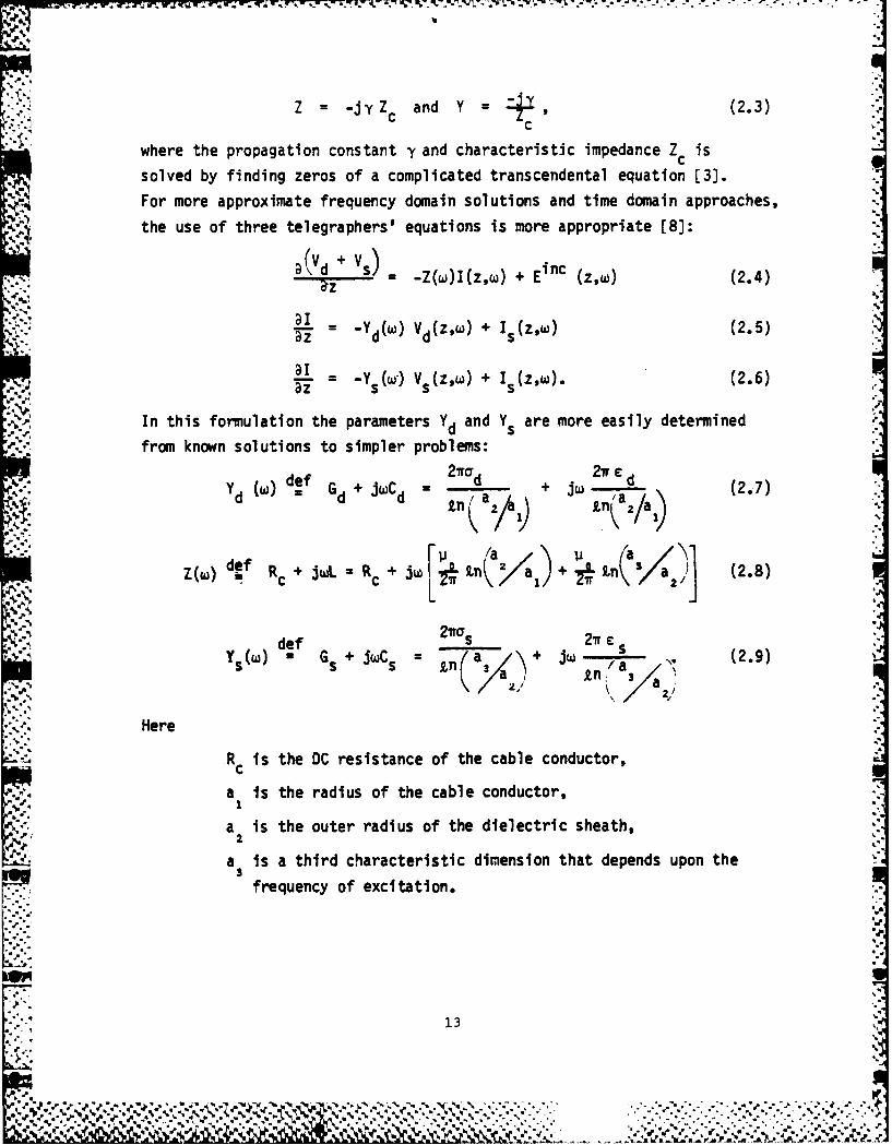
Z = -jy Z and Y - , (2.3)C Cl

" where the propagation constant y and characteristic impedance Zc is

solved by finding zeros of a complicated transcendental equation [3].

For more approximate frequency domain solutions and time domain approaches,

the use of three telegraphers' equations is more appropriate [8]:

a\ d + s -Z(w)I(z,w) + Einc (z,w) (2.4)

- -Y d(w) Vd(Zw) + is(zw) (2.5)

al --Y (W') V (z,W) + I (z,w). (2.6)

rzs s s

In this formulation the parameters Yd and Y are more easily determined

from known solutions to simpler problems:-- 21ra 2w

Y (w) def G + JdC + 21rd (2.7)

dd"d Zn a a2;7

Z(w)def Rc + iL Rc + ;/ + in 3/a 2 ; (2.8)

def s Cna(W) = G JWC5 y L.\+ (2.9)S ~~~~£ S. s n(aa +jw- aatn ~ta: aa, %f

Here

R is the DC resistance of the cable conductor,c

.4, a is the radius of the cable conductor,

a is the outer radius of the dielectric sheath,2S

a is a third characteristic dimension that depends upon the

frequency of excitation.

13

00a

v l R P .

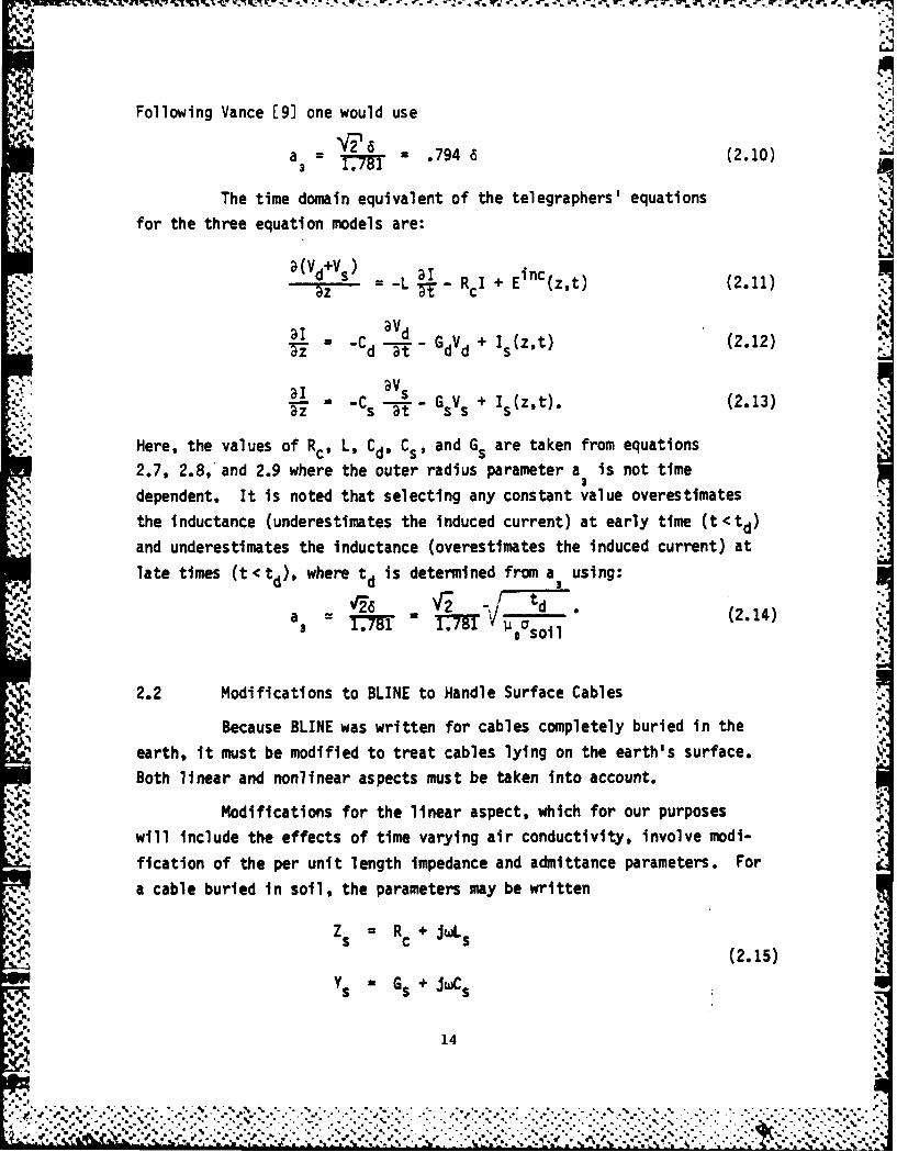
Following Vance [9] one would use

a = = .794 6 (2.10)

The time domain equivalent of the telegraphers' equations

for the three equation models are:

a(Vd+Vs) a_az-L -t RcI + EinC(z,t) (2.11)

D- lat

= C " GdVd + I (z.t) (2.12)

= -= -Cs - GsV s + Is(z,t). (2.13)

Here, the values of Rc, L, Cd, Cs, and Gs are taken from equations

2.7, 2.8, and 2.9 where the outer radius parameter a is not time

dependent. It is noted that selecting any constant value overestimates

the inductance (underestimates the induced current) at early time (t<td)

and underestimates the inductance (overestimates the induced current) at

late times (t <td) where td is determined from a using:

a __os (2.14)r~r . soilI

2.2 Modifications to BLINE to Handle Surface Cables

Because BLINE was written for cables completely buried in the

earth, it must be modified to treat cables lying on the earth's surface.

Both linear and nonlinear aspects must be taken into account.

Modifications for the linear aspect, which for our purposes

will include the effects of time varying air conductivity, involve modi-

fication of the per unit length impedance and admittance parameters. For

.- a cable buried in soil, the parameters may be written

- Zs Rc + JwL s

(2.15)

Y s GS + JWC s

14

% %%

• * "9.. - . - .- . - . . . . , o . • • .- , . - . , , , - . - . - . . . , - , . . . . . . • . . -

.4o .4... .e . ... . .. " .,.o..o " ° . - . / .. j . . ". ° "° " - "-" "° °° " ". "° " "o

", W , • , •%.• ••., . .,.* •, .•,% . ••••° °. ." , ' ." °" % " ,% % , - , % - "- ",-%

, . .. M ',V . , , , ,., . . ,.. ... .. , . ,,. . . . .- , , _.. . ,.... o,. -,. .- - . .. ,- , - , .,

Where11 .7946

" s In - aS

21T e (2.16),C 2 s I'SS C./ CS " .794 6- G CS :'G n a

In the above, the subscript s refers to the soil medium, and s is the

skin depth in the soil given by

6s(w) = - ia5 (2.17)os WUiIn order to convert to the time domain, the approximation is made that

t = 2/f [5), so that

6(t t (2.18)

4 Here, t is measured from the time that an excitation arrives at the

location of interest.

In an infinite time varying conducting air medium having con-

ductivity aA(t), formulas analagous to those for soil above can be obtained

merely by replacing the subscript s by A.

The final result for a cable on the surface is then the combina-

tion of the above results:z- 2Z A(t)Zs(t) .Zsurface ZA('t)Zs(t)

ZA(t)4 Z5(t(2.19)

Ysurface IT (YA(t)+ Ys(t)) .

These formulas then define the equivalent surface cable per unit length

impedance and admittance including the effects of time varying air con-

ductivity. They can also be applied to the case aAO, for which the limiti "s15

%

, ."., ,:'

!?:.'. 2Zs WtZsurface t

and (2.20)

Ysurface Y Y(t)

It is noted that this results in the propagation constant of the surfacecable (In the presence of nonconducting air) being equal to that of aburied cable, and the characteristic impedance of the surface cable beingtwice that of a buried cable.

In addition to modifying the soil parameters for the linearcase, the dielectric admittance must also be modified. For the buriedcable, the dielectric capacitance is simply that of a coaxial cable

formed by the soil and conductor boundaries. The same is true if thecable is at the interface between two conducting media such as conductingair and soil. However, as the air conductivity approaches zero, the radial i

electric field lines on the conductor all terminate on the soil and arenot azimuthally uniform about the conductor.

SOIL SOIL

Figure 2.2 Geometry Used to Calculate Figure 2.3 Geometry Used to ISoil Per Unit Length Im- Calculate Cablepedances and Admittances, Dielectric Admittanceand Cable Dielectric Admit- for HAB Case.tance for Conducting Air.

Thus, for the time varying conducting air medium above the soil,

p. the geometry of Figure 2.2 can be used to compute all cable parameters. U,.

;'

16

00 N:V" " " % "' " . ', .' - " " .",'.'.'',".' -' - ., ---*.,- -. -** ' -,"-"." " .- -. ,,.. .

9MCF.M, . -. . .TV .. .. ij

However, for no air conductivity (the HAB case), the situation

is somewhat different. A surface cable would not be deployed in the

manner of Figure 2.2, although that is the correct model for source

region computations. (In the presence of conducting air, the radial

field lines should be azimuthally uniform, even if deployed like Figure

2.3.) A surface cable would be more nearly deployed in the manner of

Figure 2.3. It is clear that in this case, the dielectric capacitance

is determined by the geometry of a wire over a ground plane. This also

means that the radial electric field is not simply that given by coaxial

geometry as in the BLINE case, but is given by the wire over a ground

plane geometry, Figure 2.3. The electric field is therefore a maximum

on the soil side of the conductor, and minimum on the top.

The nonlinear aspect of BLINE to be modified for surface cables

involves the treatment of soil breakdown, whereas the dielectric break-

down is unmodified, that is, dielectric breakdown is treated as a hard

short.

For a cable buried in the soil, the ionized soil region is r.

roughly spherical (except for a bicone coaxial with the cable) and the

radius is determined.by the soi l breakdown electric field, which is 1-2MV/m.

For a cable on the surface of the earth, an arc to the earth will form a :-':

region roughly the shape of a thin disc, because the surface breakdown of

soil (250-500 kV/m) is much less than that of the bulk soil medium. There-

fore, the ionized region tends to extend along the earth's surface instead

of into it [10.

The ionized region is treated as a thin disc of radius rarc,

where rarc increases until the electric field at the edge of the disc

is equal to the surface breakdown field EBR. For a current I flowing

into the disc, rarc is determined by

arc c

17

." %*..*.***.. * . . . .. .V .~~~ . q; -.-.. , .; . -. ..-. .-.:. ...,.....:..>..- .:.. ...*..*.. ......:,*......* . -* * * .**... . ..- ,..,.. .. . .,:..

from which one obtains

rarc V sE (2.22)

The disc then has a conductance Garc and capacitance Carc

given by

Garc = 4as rarc

(2.23)Carc 4srarc:

The relationship of the conducting disc to the TEM transmission

line surface cable code is Illustrated in Figure 2.4. In order to ensure

that rarc is never greater than one-half the spatial increment Az, rarc

is set equal to the smaller of Az/2 or rarce

It is noted that the soil may break down before the cable

dielectric does. When the dielectric punctures, current flows through

the puncture into the soil forming a disc as previously described. How-

ever, when the soil breaks down and the dielectric does not, the concept

of the disc does not apply because the current flowing into the soil is

distributed along the cable length and does not flow from a discrete

point. In this case, the soil nonlinearity is treated differently as

discussed in the following.

The cable geometry of Figure 2.2 is assumed. The ionized soil

region will then extend into the soil a radius of a until the electric

field is equal to the bulk breakdown field of the soil. This breakdown

field is then given by

VsoilnR (2.24)

a

18

% %S

o,,

cablesoi I

L -

+ R, Az .surface.

Cable DielectricD Capacitance and

Dielectric Break-down Switch

r (Az-2 rC), -surfacesurfac

- (Az-2 r arc)surface r arc

Disc Admittance

.-2....

Soil Admittance /

Figure 2.4 Illustration of Surface Cable Soil Breakdown andIncorporation into TEM Transmission Line Model.

%% % %. .. -19 q

This equation can then be solved for the new radius a'. However,2

because it is a transcendental equation which must be solved at every

time step (a time consuming process) an approximate solution is used:

1 'soila = (2.25)

2 ELn aEBR a

al

2

where a' on the left hand side is the new value and a' on the right handz

2side is the value obtained from the previous time step. The solution isstarted by letting a' initially be equal to a

2 2

The computation of the electric field is also necessary in order

to determine dielectric breakdown. For the coaxial case. the maximum

electric field E in the dielectric having a potential V across it is

given by

V (2.26)Emax "a

a Ln *i32, a

for the wire over the ground plane case, it is given by

E max 1(2.27)Emax cosh- 1 a .'

a

where X= a -a

!d aZ Ka i211a a5

a

-.

02

'20

A

- ........k 'N L , Y,: , ,, '. ':, " : : .,', ;' €;*,*. .K'.:'';',-L -;. ";; . ;-'- '"':'"'.''.-' .'.-'

SECTION 3

RESULTS OF SURFACE CABLE COMPUTATIONS

3.1 Background

One of the goals of the study was to perform surface cable

computations for several cases, with and without including the nonlinear

effects. Table 3.1 summarizes the cables studied, the soil conductivities,and the environments used for the parameter study. Both linear and non-

linear predictions were made in order to ascertain the effects of including

nonlinearities.

Table 3.1 Surface Cables for Parameter Study

Length Environment Soil Conductivity (mho/m)

100 m HAB Overhead .005HAB Overhead .01Tactical EMP .005Tactical EMP .01

600 m HAB Overhead .005HAB Overhead .01Tactical EMP .005Tactical EMP .01

2800 m HAB Overhead .00 5HAB Overhead .01Direct Hit at End of Cable .005Direct Hit at End of Cable .01

The surface cables studied are formed by the shield and outerdielectric jacket of RG 58 and RG 8 cables, whose dimensions are indicated

in Table 3.2.

21

°a

V, "..'... : -.,s% .- :.. :.:- . .,- . .. .•. ".' . ,"" %.." ,- - - '. - . "" ''" " " " ' .

Table 3.2 Dimensions of Cables Used in the Study [11].

Cable a (m) a (mm) Dielectric Thickness (mm)

RG 58 4.276 4.95 .674

RG 8 9.209 10.29 1.081

II ,I ! / _ _ _ __ _ .

a. wire over a ground plane b. wire in conducting medium

Figure 3.1 Geometry for Definitions of Radial ElectricFields.

Table 3.3 Constants Used to Multiply the Dielectric

Voltage to Obtain the Radial Electric Fieldat the Points Defined in Figure 3.1

Cable Ea Eb Ec Ed Ee Ef

RG 58 187 262 1670 1408 1276 1752

RG 8 92 118 1006 888 824 1043 %Z

The radial electric fields are computed by a constant which

multiplies the dielectric voltages. Figure 3.1 and Table 3.3 define the

constants at the locations indicated. When this constant is multiplied

by the dielectric voltage, the result is the electric field at thatlocation in volts/meter.

The cable jacket material Is polyvinyl-chloride (PVC). In

order to do the nonlinear computations, it was necessary to determine ',

what the dielectric strength of PVC is. Several values were found in

the literature and are summarized in Table 3.4. It is clear that values

vary widely and depend upon the types of material, thickness tested, and

test waveform. Values for polyethylene (PE) are included for reference

22

--

, . . - . - .. . -. - . - , . # .. ..- .% . . . .

4,. • . ,.. : ... . .... . , ... . , . ....... ...*. - *.*..

-- -3-1 W- *S7 - -

purposes. It is troublesome that the relative dielectric strength of

PE and PVC varies considerably from source to source. The problem is

compounded by the fact that for the purposes at hand, it is desireable

to have a value which applies to a voltage which rises in a few hundred

nanoseconds and is gone nominally within one or several microseconds, and

probably none of the data in Table 3.4 applies to this time regime.

Table 3.4 Summary of PVC and PE Dielectric Strength

Data from Various Sources. Units are volts/mil.

Source PVC PE

Reference 12 375 420-550

Reference 13 400

Reference 14 600-1000 iflexible) 460700-1300 (rigid)

Reference 15 800-1000 460Reference 16 800 (AC) 1200 (AC)

2000 (DC) 3000 (DC)

Extensive data has been taken on PE breakdown and is summarized

in Reference 17. This data shows that for lightning type pulses (1h x

40 usec), a conservative value to use is 2000 V/mil. It should be noted

that some data exists for even shorter pulses (1 x 5 psec) which yield a

5000 V/mil value [18J. A value of 2000 V/mtl was used in other buried cable

studies [5). If one assumes PVC behaves similarly to PE and uses the data

from Reference 16, one obtains a value of 1330 volts/mil for PVC. It is

admitted that this is a guess based on conflicting data, and if one is

going to perform some experiments involving cable breakdown, one should

first obtain the dielectric strength data for the time regime of interest.

It is noted that cable manufacturers were called, but they have no data onthe jacket dielectric strength.

23

nea .,'• . .,, -. ... ..

3.2 Computations for the High Altitude Burst (HAB)

The threat for the HAB predictions was taken to be a plane wave

normally incident upon the earth and polarized parallel to the cable.

Previous work which investigated angle of incidence effects showed that

end-on incidence results in only one-half the response of normal incidence

" ~*[3], and responses for other angles of incidence yields values within one

percent of the normal incident case, so it is felt that normal incidence.JI

is the appropriate case to study. The temporal behavior of the plane

wave is the familiar double exponential

Einc z 52 (e" 4x 1 - e" 4.76 08t ) kV/m (3.1)

Standard plane wave reflection coefficients were used to obtain the total

field at the earth's surface, which is shown in Figure 3.2 for the two*values of conductivity used in the study. The cables studied were shorted

on one end and open on the other.

24

a 0.005

S18

-- " -- '-- - - - -_12

6 .0.0i

4~. 0.

0 40 80 120 160ns

'p...I!-SFigure 3.2 Total HAB Electric Field at Earth's Surface S

24

* * % I

.'i ,", " "" "-" "." "" """, ."" ,''- "" ". " -""' "" '"" "*"-" " "-"5". . .- .- .".-*-"-* - -'t.' \-. -"-5- -" -. V-"'"

HAB results are summarized in Figures 3.3 through 3.8. Some

general remarks can be made about the HAB results. First, it was found

that the results for lengths 100 m or greater were independent of length,

within 1%. That is, the spectral content of the HAB input is of suffi-

ciently high frequency so that signals propagating from one end toward

the other attenuate rapidly and are not discernible at the far end. This

is evident in Figure 3.3 which shows the short circuit current. The

response from the other end should be arriving at about 700-800 ns assuming

a nominal propagation velocity of one-half that of light, and it is clear

that no such signal is there.

The second observation is that the voltage induced on the RG 8

dielectric is insufficient to cause breakdown (52 kV is required), and

RG 58 breaks down only for the case a = .005 mho/m.

From Figure 3.3 it is evident that the nonlinearities (both

soil and dielectric) do not make a significant difference in the shortcircuit current response. For this case, only the three cells closestto the open end broke down, and this effect is not felt at the shorted

end nearly 100 m away. The three cells closest to the open end broke

down at 267, 172, and 270 ns, ordered in the direction from the shorted

end to the open end, respectively. '-

It is also evident that the soil nonlinearities (which occur

even if the dielectric does not break down) are unimportant in the

current response as evidenced in Figures 3.3 and 3.6. It also makes

little difference in the soil and dielectric voltages as evidenced in

the RG 8 responses of Figures 3.7 and 3.8, which show essentially the

same response for linear and soil nonlinear cases.

For the case in which the RG 58 dielectric breaks down, the

voltages across the soil and dielectric are quite different from the

linear case as one would expect, and this difference is evidenced in

Figures 3.4 and 3.5. It is noted the end of the cable was artificially 1.

forced to be open, which is why the dielectric voltage of Figure 3.5 does

not go to zero. -.

25

25°-.

2 s i,.-..'.

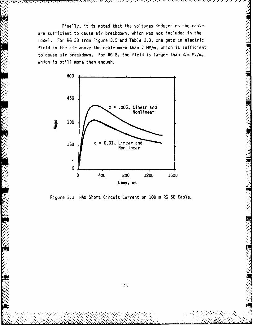
.5- Finally, it is noted that the voltages induced on the cable

are sufficient to cause air breakdown, which was not included in the

model. For RG 58 from Figure 3.5 and Table 3.3, one gets an electric

field in the air above the cable more than 7 MV/m, which is sufficientto cause air breakdown. For RG 8, the field is larger than 3.6 MV/m,

which is still more than enough.

600.

- 450

.. oa .005, Linear and.... Nonlinear

,..' 300

NE

150 a = 0.01, Linear and"*-'" Nonl inear

0 400 800 1200 1600

time, ns

Figure 3.3 HAB Short Circuit Current on 100 m RG 58 Cable.

.".

26X4..

S . . . . . . .* - .-.. . .

20~

40

I~C 0.00005Liea

-404

0 100 200 300 40

ns

Figure 3.4 HAB Soil Voltage on Open End for 100 m RG 58 Cable.40

a =0.005, Linear

CY~U 0.0

.4 ~30o0 0Linear &

0.0 Nonlinear

Nonlinear20

a10

10

Fiue0 0 460 860 1200 160

Figur 3.5HAB Dielectric Voltage on Open End for 100 mn RG 58

800.

600.

z 04000

0

0 400 800 1200 1600ns

Figure 3.6 HAB Short Circuit Current for 100 m RG 8 Cable.Linear and Nonlinear.

40.aI

a=0.00530

,..2 0.

Jr

Figure 3.1 HAB Soil Voltage on Open End of 100 m RG 8.. . . . . . .. . . . . . . . . . . . . . . . . . . . . . . . . . . .

440

/ x*5N aO0.005

'4 .~20 .

10'

0~0

0 400 800 120 1600

ns

Figure 3.8 NAB Dielectric Voltage on Open End of 100 m RG 8. .Linear and Nonlinear.

3.3 Computations for a Tactical Environment

The tactical environment which excites and influences the cableresponse is the radial electric field and the air conductivity. HDL sup-

plied waveforms for these variables at ranges from 50 to 2800 meters which

were used in the computations. Typical waveforms are shown in Figures

3.9 and 3.10 which are for a range of 1000 m. Cables of 100, 600, and2800 m length were studied. In all cases, they are oriented radially to

the source, and the end closest to the source is a perfect short and the

end farthest away from the source is open circuited (except for one 2800 mcase, discussed later). Responses computed are the short circuit current

at the shorted end, and the dielectric voltage and soil voltage at the

open end.

.P

29

p.b

5,. . . . . p ., ,.5,, , .*....-. ,r . ," ,.. A ,S." ., , , . .. 'v ,.. .'S .,_.-- * .S.,? ', ,...,..-.-, .- ,..-....-.-,.....] .

3000

2500"

2000.

-. 4., 1500.

" ~ ~1000./'.'

N1 500 1

Soo,

04............................ ..

10 10- 10 101Seconds

Figure 3.9 Tactical Radial Electric Field at 1000 m Range. .0

20

16 I.

J,12

4

0 ,.. . . .... .. .. "10"-1 " 10" 6 10"-1

Seconds

Figure 3.10 Tactical Air Conductivity at 1000 m Range.

30

V.

*4.''' . , , . C ,, .. . , " """ . . . ."."."."-"- '. . , .-. ", , ,- ,",-. * , ... ' ' ' .' ' ' -. ,. ' ' .: . ' .. ; '. .,"

..... , ..,.,., ,... ... .... ...... ...... .., . .. ., .... . .,. ..... .., .... .._ ,. ... .,.. .,.. .-..... ...-, ....,:..

Results for the 100 m cable are shown in Figures 3.11 through

3.16. The cable is located between the ranges of 900 and 1000 m. The

effect of the nonlinearities is to greatly increase the short circuit

current, as shown in Figures 3.11 and 3.12. The late time ,:4ponse is

also greatly extended. The effect of nonlinearities on the soil voltageis to reduce it and significantly alter the spectral content as evidencedin Figures 3.13 and 3.14. Of course, as one would expect, the effect of

the nonlinearity is to greatly decrease the dielectric voltage.The propagation of dielectric breakdowns for the 100 m cable

is interesting. For example, for the RG 58 at a - .005, the dielectric

breakdowns begin at the open end at t - 1.63 usec and propagate a distance

of 38.7 meters toward the source, at which point breakdown occurs at 7.95

usec. It appears likely that if the computation were extended in time,

the punctures would propagate even further.

Results for the 600 m cables are shown in Figures 3.17 through

3.22. One end is at a range of 400 m and the other is at 1000 m. Results

are similar in character to those of the 100 m cables except that the

responses are much larger. The propagation of dielectric breakdowns is

more complex in this case than for the 100 m case. For RG 58 at a - .005,

the first puncture occurs at 92 meters from the shorted end at 3.23 usec

and propagates both directions; inward to 74 meters at 3.3 usec, and then

outward every 6.6 meters (approximately). In addition, breakdown occurs

at the far end at 3.37 isec and propagates inward a distance of 66 meterswhere breakdown occurs at 12.6 usec. The end result is a complex pattern

of punctures which is non-uniformly distributed along the cable. Thereare no punctures at distances closer than 74 meters to the source end of

the cable.

31

-r w ............... . .-...... ......... -

*0.0

Nonlnea

0 3 0

3.00a~~~.0 Li.0nNnlnerar00

Nonlnea0Linear Lna

-4 1

0 9

-3.0..1

0~~~ 3 9 1

%4

4.-3.0

'3 12'

Sd. ~ . ~ ~ ~ N. ~ **l*,*u.s*

6. . . . . . . . . . .

a 0.005, Linear

0_

~;s y 0.01, Non~ ear

-8

-16 __ _ _ _ _ _ _ _ _ _ _ _ _ _ _ _

usec

Figure 3.13 Tactical Soil Voltage for 100 mn RG 58 Cable.

204 =0.005, Linear

a = 0.01, Linea-

j ~ ~ Non inea r0 _ _

Nonlinea-10

0 39 12jisec

Figure 3.14 Tactical Soil Voltage for 100 mn RG 8 Cable.

33

200wa0.01,

Li neara0.005,

150 Linear

100

V a *0.005, Nonlinear

50

a *0.01, Nonlinear

%p. 0,

0 3 6 912

wisec

Figure* 3.15 Tactical Dielectric Voltage for 100 miRG 58 Cable.

200 0 0 , L n a

a 0.05 0.0neLnea

150.-=005,Lna

100

50-a 0.01, Nonlinear

0p

0 3 6' 9 12'

Figure 3.16 Tactical Dielectric Voltage for 100 mRG 8 Cable.

34

5,, II-.5.~Il , - *.

5....6.

12.

,-S.

a 0.01, Nonlinear--

*1 4

a .- 0.00. Non-

"

,.( li near

8 a=0.01, 0= .005,i ~ Linear Linear ..

0 4 8 12 16

I.'Sec

Figure 3.17 Tactical Short Circuit Current for 600 m RG 58.

16 m ';

1 6 0.01, Nonlinear

12 a= 0.005, ton-0 = 3.01, linear

Linear a=0.005,LinearLinear

-8 .

4a4

0 12 16

vi sec S..

V Figure 3.18 Tactical Short Circuit Current for 600 m RG 8.

35

ki .:.%

- - =0.005,

'Oe 00, N \Linear

10 l a 0.01, LinearV 10-

* 0.005, Non near

91,pS 0,

a 0. 01 , Nonln

-10

-20 ____________________

pisec

Figure 3.19 Tactical Soil Voltage for 600 m RG 58.

20

~ \ Linear

a0.01, Linear~fl

lv av100,1

0.01 0,lie

-20a

ii Sec

Figure 3.20 Tactical Soil Voltage for 600 m RG 8.

36

e %

% a%

'400-

a=0.01 & 0.005,Linear

300-I,

100- a 0.005, Nonlinear

0 a 0.01, Nonlinear

0 4 8 12 16

iisec

Figure 3.21 Tactical Dielectric Voltage for 600 m RG 58.

400a*0.01, Linear

300-

a=0.005,

100. a =0.005, Nonlinear

a =0.01, Nonlinear 6.

0 4 8 12 16

iusec

Figure 3.22 Tactical Dielectric Voltage for 600 m RG 8.

7W 7 7

Results for the 2800 m cable are given in Figures 3.23 through

3.28. Cable currents are similar in character and in amplitude to those

for the 600 m cable. The effect of the nonlinearities is to greatly

increase the late time response. Also, the nonlinearities greatly reduce

the dielectric voltages and significantly alter the amplitude and wave-

shape of the soil voltages.

The pattern of dielectric punctures is quite complex for this

case also. For the RG 58 with a = .005, the first puncture occurs at

280 m at 3.18 usec. The puncture closest to the source is at 60 m and

occurs at 3.3 usec. The far end breaks down at 13.8 usec, but this is

the only puncture in the last 500 meters of the cable. The remainder of

the cable has a complex distribution of punctures.

For all of the tactical computations, voltage levels are

higher than those obtained for the HAB case. Thus it is clear that the

air will break down also, an effect not included in these computations

but which should be considered in the future.

Because there is some interest in knowing what the short

circuit current at the far end of the 2800 m cable is, it was also

calculated (with both ends shorted) and is shown in Figure 3.29. It

is noted that the linear and nonlinear cases agree. This is because

there is no dielectric breakdown in the last 500 meters of the cable,

and the effects of breakdown are not significant by the time they

propagate to the far end.

,V-.1111l38

i -;t"''-,,'. :'. .'."-';" ' .:-,; ,";"..-;"-.,;;.*..;,.-, ",- ." . . . ,' -*- •-.-; , ,,,.-;-;."

i .•:'K<."j > *vv -V -" l.*~ . . -.' * -i -/l , ~

. t a * ~ . . . - . . .- a a a.. . + . : - . ' . .- . - . ' : 2 - " ' . -'- ' -

, ' % oL .

-- ,-. . 77

16 ' 16'

12 0.01, Nonlinear

aZ 0.05 •Nn

s12.

cF .. 0L

58 ~ a0.00005Liea

.. : .0 id 26J 36)

jisec

Figure 3.23 Tactical Short Circuit Current for 2800 m, .. : RG 58 Cable.

!"12 Nonl nea = 1 a" ( 0.005, Nonl i... ..

NNonline"~ - 0.01, Linear

-~12.005

-dL i near.-,J

"8.

-...

0 10 20 30 40

isec

Figure 3.24 Tactical Short Circuit Current for 2800 mq RG 8 Cable.

54

.. . . . . . . . . . . . . .. . . . . . . . . . .p * V a a / . K * . a. . . . , .• . . . . . . . . . . .

a -+,, . i, . .. a.,, , ,: . . . . - . . . . .r',, .,. - .- a , .: %*>,,,. ": .. ,,. . ,,,, ' ,- -v -...- .. '-.--

10.

y = 0.005, Linear

5 a = 0.01, Linear

~~0

= 0.01, Nonlinear

a = 0.005, Nonlinear

-10 __ _ _ _ _ _ _ _ _ _ _ _ _ _ _ _ _

0 10 2d 30 40

usec:Figure 3.25 Tactical Soil Voltage for 2800 m RG 58 Cable.

:'-4";. 20pI, .

'ph.. 20'

10a.= 0.005, Linear

a'=, = 0.02, Linear

-> a

.%. a = 0.005, Nonlinear

-10

1/ :,

-20 "_"

0 10 20 30 40

Slsec

Figure 3.26 Tactical Soil Voltage for 2800 m RG 8 Cable.

a,,* 40

a-'

60'

a=0.01 & 0.00O5Linear

45

~30

a 0.005, Nonlinear

15 a, 00.01, Nonlinear

0 10 20 30 40

lusec

Figure 3.27 Tactical Dielectric Voltage for 2800 m3' RG 58 Cable.

60 =0.01 & 0.005,Linear

40 0. OC 5

40 INonlinear

50.01,20 Nonlinea

0

. W.

-200 1 0 20 30 40

i.secFigure 3.28 Tactical Dielectric Voltage for 2800 m

RG 8 Cable.

41

_ , I~000 ,,i €

'.. 750"

SLinear andNonlinear

250 _.

0'.

0 10 20 30 40

Fu 3 So C usecFigure 3.29 Short Circuit Current at the Far End of the 2800 m

RG 58 Cable. Ground Conductivity is .01 mho/m.

4?42

?.,. r "

a.-9,..,

-9.9- -V,'-.-.%

-V.

- 42,..:::: .

".% .- " %. .". '- - " % %' %i.-.%.",,'. . " *.%.% %.% '. % % %".."% ' % . - -. • - .. . . -. , . , ., • - . ,. - % ..a . ' , . • . " W "-.- "1% ' . " % ' . • " % % % % * ' . * . . • " " * •

--V. -- ", " . " , * , " . "- - . " " % % , % ,%"a,% . " . " . ", " ' . - - ' . -"." - ".'9.4 ' ,-. . ' ' ' -< :-.,. _:..,' . . - . ' * . , ...... ,-..-i'.'.......,-'-.,,,'

SECTION 4

EXPERIMENT FEASIBILITY

C-.4.1 Background

One of the goals of this study was to determine the feasibility

of using existing simulators to investigate nonlinear cable response.

v Computations were done using AESOP, which has the same electromagneticcharacteristics as TEMPS, as the source of EMP fields to illumine the

cables into their nonlinear response regimes-. It was found that AESOP

can indeed be used to perform these experiments. In order to do this

study, the electromagnetic field model of AESOP had to be determined. 'C

Then some experimental concepts are given, and then some computational

4..,

results are shown.

For the purposes of this section, three cable responses were

computed, both with and without nonlinear effects included. Figure 4.1

illustrat~is the type of cable configurations that were studied. A smallcoaxial cable like RG 58 would make a reasonable test cable for theinsulated cable and 1/2" electrical conduit would suffice for the uninsu-

lated conduit.

The three experiments include most of the interesting effects.

The U-shaped insulated cable will exhibit a voltage maximum at the base

of the U. If breakdown occurs, it will begin in the U-shaped region.Several punctures of the dielectric are likely to occur. The principal

question is at what minimum field intensity will a puncture of the

insulating jacket be obtained. Additionally, one would like to know theperiodicity of breakdowns along the cable in the case where a very high

* field intensity pulse is applied to an undamaged cable.

43

z .

.-

*~~' ... '-

4 ,.-.,"I - ..-

• 1...

2 0

SSa

i.4 EUT

1 go

_ ___ -.-._

L "I

LA..

keU

44 0

• • . • . '. . . . -' . ) ...' . o - .' . . . . . % ' " . . .. . "% , % ' . % " " .% " * % % • .. " . . " . . • • . " .' . . . . . .. . . .' ' " a -. "

..., -. ,.,.',,..',.- ., ,,;',' -, -j _, ,,.,. - -,:, ,,," . ,, ,,., .. .. .. . , ,. , .. , ... ... ..U. • . . ..U.

The uninsulated conduit will be a test of our understanding

of the nonlinear response of soil, unconfused by the mixing of dielectric

breakdown and soil breakdown.

The ground stake experiment will examine the ground stake,. response as a termination impedance. This tests directly the model of

nonlinear incremental soil parameters without including distributed

parameters and distributed sources in the analysis.

4.2 The AESOP Field Model

The model used to predict the fields is the same as that of

Reference 19. The electromagnetic fields produced by AESOP are much

more complicated than the high altitude burst plane waves. For AESOP,

the amplitude, angle of incidence, and the wave polarization are a

function of position, whereas they are not for HAB.

Figure 4.2 shows an oblique view of AESOP and the coordinate

system. The antenna is on the z axis at y - x = 0. It is 20 meters abovethe earth. If one draws a vector from the origin at (0, 0, 0) to another

point (x, y, z) where the fields are to be defined, it is useful to define

the angles a and 0 according to the following: '.Z

cos 0 z

;2+ y2 + Z

(4.1)cos *4* -fit + y 2'1

The radiated fields are found from the formulas of Jordon [20)

for fields near a dipole and are expanded in a power series to obtain%5"

the fields before reflection from the ends take place. This is equivalent

to making the antenna infinitely long, or else having a long antenna withperfectly matched terminations on each end. Iq

45

. . - , " " ", . , " "', . . . . - - --N

%U.

* 'r *-2 ~ e, -e e%~~.'p p%. .'%

-0o -. . -

A 4Ar_

46)

S.or.

1.7:

The resultant total electric and magnetic fields areV0 'Et 0

Sand -E (4.2)

H t

0

where V0 is the pulser voltage and Vip s a constant, and are chosen to .*

normalize the incident electric field to 50 kV/m at the earth at theScoordinate y = 50 m. The field and its spectral content are shown in

Figure 4.3 and 4.4, respectively.ia A

The unit vector U perpendicular to the plane of incidence isp '

wiu' given by

A rA A.4- 2 U z (sin$ cos) - Uy (cos0) (4.3)P Vs insco + Cos

Then the incident horizontally polarized and vertically polarized inci-

dent fields are given by

K Etcos A-

IN4C (sinas cos*+ cos20)l/2

E HyEt sin cos.".(.4HVPINC n0 (sin 2 cOs 20 + cosz8)l/ 2 U /

An approximation is made that the plane wave reflection co-efficlents [21] for the earth can be used. The total field parallel to

the surface cables is then computed and used as the excitation source

which drives them. The earth is assumed to have constitutive parameters

9 = 10s and a = .005 mho/m. The risetime of the AESOP field can be in

the range of 4-12 ns., and a nominal value of 8 ns was used in the compu- '.:

tations.

"° 4

li 47

. . .. .. .. . . ..

50

90.5

90.4

0.2.

0.

o~ns

0.540.43

0.32

4 48

On 0.

ME

4%

Figure 4.5 shows the total electric field at (-20, 3, 0). It

was found that along a line from this point to (-20, 3, 37), the total

electric field did not noticeably change waveshape and the peak amplitude

decreased nearly linearly (within 3%) to a minimum of 45.2 kV/m. This

line is the line upon which all of the cables to be studied were placed.

60

50

*40

30

10

b LU

0 -%-

0 250 500 750 1000

ns

al'

Figure 4.5 AESOP Total Electric Field at (-20, 3, 0).OS

all

49

L x.

0 250 50 750 100...--

. . . . . . . . . . . . . . . . . . . . . . . . . . . .

4.3 Results for the Ground Stake Experiment "-"-"' The ground stake experiment consisted of 37 meters of RG 58

with its shield terminated to a 1" OD ground stake of length 2 meters

and the other end open circuited. The ground stake impedance is 98 -r%.,

according to the formulas of Sunde [10]. Figure 4.6 shows the stake

current and Figure 4.7 shows the dielectric voltage at the other end of

the cable for linear and nonlinear cases.

The current shows a small nonlinear effect, but it would benoticeable on a measurement. If one could measure the dielectric voltage,

a marked difference could be observed.

400 ~L inea r

300.... $:

~Nonl inear"."

200 .

100.

l0

0 200 400 600 800•

ns

Figure 4.6 Stake Current.

505

r '.,- ,- .,-.-,o ..* .. .- *...-.- ".- -... : . . -- .. -.. -... -. - . - -..-. - .-- - - - -- ,- -- . -F : . -. -. : -',: -'..'-,-,'-.--.-.-. " - .-. -. '.. -'-. . -. -.-..5*J %-. ,', ,-,'-v..,% %- .;, ,-,-,.,' ,,,

P' .. . .. *. ' I ' ' '

,-W ° " % ,". ," " _ % " _" " ' - ' .• .

, _" . " - "..= , _

q -

.

47 - -

80--o-

Linear !';l

60 R*..

40- Nonlinear

2~ 0

20

0 200 4do 600 800n sFigure 4.7 Dielectric Voltage at End of the Insulated Cable.

The computations indicate that the 7 meters of cable closest to the open

end would experience multiple punctures. The first puncture occurs at -

the open end at 84 ns and the punctures propagate 7 meters and the last

one occurs at 330 ns.

Because punctures occur only at the end away from the stake,

their effect on the stake current is rather small. A shorter cable wouldprobably cause a bigger difference in stake current, but even that in

Figure 4.6 is discernible. From Figure 4.7, one may conclude that if onereduced the simulator output by a factor of 2, the nonlinearities would

just be at the threshold of occurrence.

IAN

51

-I% --

.*. 1* * -. * **. .~F.'.. . . .

4.4 Bare Conduit Experiment

Figures 4.8 through 4.10 present the results for the 37 meter

long bare conduit computations. These results are consistent with pre-

vious results in that only small effects in cable response are causedby soil nonlinearities. The results shown are computed from a much

S'... reduced value of bulk soil breakdown voltage: 375 kV/m. This was done

because if one used 2 MV/m, the results nearly overlayed each other and

it was desirous to ascertain the importance of the soil breakdown field.

It appears that the non-sensitivity of response to soil breakdown above

can be readily checked by this experiment.

.°

_. = 800 !I

600.," -. Lia ear

1-400

200

',' 0

0 200 400 600 800

ns

Figure 4.8 Conduit Center Current.

5, 52

.-''.....

4

%" .o .S

*-5o• , . , • ,5 ° , . , . o o .o . • . o ,. \ o,. . . .,' , ,- --, .- . .. . ...... . .' - .o' * *',W -,*5., ft ,"-.. • " "-"" " "" "" S '' F

" ' '-

'

80

Li near60

40 NonlinearN.

20

2 200 400 600 800'ns

Figure 4.9 Voltage on Left End of Conduit.

80 .

4

60 Linear

20

0 200 400 600 800

nsFigure 4.10 Voltage on Right End of Conduit.

53 4.

4.5 "U" Cable Experiment

The "U" cable is 37 meters long on each side and the joining

part is 6 meters long. The cable is open on the ends. Its response is

predicted to show the most dramatic nonlinear effects. Results are

presented in Figures 4.11 through 4.16.

The current response (Figures 4.11 through 4.13) should be

easily measurable. The effect of the nonlinearities is to greatly increase

the peak value and late time currents as shown. From the voltage waveforms,

one can estimate that nonlinearities would begin to occur at about 50% of

simulator output.

300.:. ' Nonl inear

200.

100Li near

.! 0

0 200 400 600 800

nsFigure 4.11 Current at Corner of "U" Cable.

4-

..

.5. , 54- , " .=. . # . . . , . .

e% .-.%*C *..:: ,...;.--/:,.:.-..%........5 -.-..... ... .*.....,....,... . ... ;

800 4

600-

Noliea

400-

200-

0

0 200 400 600 800 Li

Figure 4.12 Current Midway Between Corner and Endof "U" Cable.

-I 400

4 300.

200.*41

N 100

0

-100I:0 200 400 600 800

ns

Figure 4.13 Current 1.3 Meters from the End of the"U" Cable.

55

%i 0

80

60 Linear** ':

Ac40-ea

-*' 5

20Nonlinear

0.200 400 600 800

ns

Ficure 4.14 "U" Cable Corner Dielectric Voltage.

:. ." 80 ,

q '::60. Linear

S40-

20- NonlInear

-..

0 200 400 600 800

ns

Figure 4.15 "U" Cable Center Dielectric Voltage.

561

• , ,. ,,... ,,.,.. .... . .. -. . J,, . . . . .. " ." .. . . . . . . . . . " ." - -. -" -- -" ..... .", -' c-" . - , ,

...- 'L ' " , y .,' x

Sr , *, , _ .a _ - . ; , . -- . . . . . : ...S. .:o .

S.,

Linear

60-

.. 40 - Nonlinear

20-

0

0 200 400 600 800

ns

Figure 4.16 "U" Cable End Dielectric Voltage.

For the "U" cable, the punctures are in the vicinity of the

corners and at the open ends. At each open end, a puncture occurs at

155 ns and punctures propagate away from the end a distance of 2.6 m,

where the last puncture occurs at 491 ns, (time measured from when the

incident wave arrives at the corner of the "U"). In the cable region

between the two corners there are numerous punctures which occur between

153 ns and 177 ns. It is interesting to note that no punctures propagate

away from the corners towards the open ends.

*-p. .pj

U 57

%.. ..... .. . ...... .. . ............. .... ........

SECTION 5

CONCLUSIONS

This Is the first known attempt to estimate the effects of

soil and dielectric breakdown upon surface cable transient response,

and the results need to be subjected to careful experimental comparisons.

However, the analytical results indicate several interesting conclusions:

1) The effect of nonlinearities is principally to greatly

increase the late time currents and reduce the voltage delivered by a

cable (for the tactical case). This means that the effect of nonline-

arities on system response is to reduce the voltage on high impedance

systems and to increase the current on low impedance systems. Of course,

a high impedance system may itself break down and become a low impedance

system.

2) HAB results were not greatly affected by nonlinearities,

at least for the cables studied. More dramatic effects might be observed

on wires with thinner insulation, such as field wire.

3) The most important nonlinearity is cable dielectric break-

down, whereas soil breakdown is of minor, and sometimes negligible,

importance.

4) The results clearly show that nonlinear air breakdown will

occur in the vicinity of the cable for both HAB and tactical excitations.

This effect should be evaluated as a next step, especially before performing

experiments in TEMPS or AESOP.

5) One of the most important unknowns is the dielectric break-

down of cable insulations in the appropriate time regime. Data from the

literature and handbooks is incomplete and conflicting. It is felt that

the parties concerned should take their own data in order to have confidence

in it.

58

1

4 5~ 4~, ~ 4, ' - .....

4 .. . . .4 -, , . , w . , , .. ,. . . . - - . . .,. . . . . . . . . . L " . . . . ." . ._

6) AESOP or TEMPS can be used to validate the nonlinear

analysis tools used in this study. Computations show that the important

features of nonlinear cable response, such as the late time large current

and the relative importance of the soil/dielectric breakdown, can be

determined.

7) It is noted that results were presented for a cable "ideally"

located at the earth's surface. In reality, a cable will perhaps be

touching the earth's surface at only randomly selected points, and will be

slightly elevated for random intervals. Results should be computed for

other representative geometries.

It should be pointed out that there are several assumptions in

the model which may require further research or verifications. Among". these are:

1. The value for the soil breakdown fields.

2. The temporal behavior of soil breakdown (that is, itwas assumed that the soil broke down without timedelay, once the field exceeded the breakdown value).

3. The validity of the "disc model".4. The "disc" radius was limited to be one-half of a

spatial finite difference increment.

5. The value of the cable dielectric breakdown fieldsand their temporal dependence.

6. The validity of the model used for soil breakdownwhen the dielectric did not. (Surface flashoverwas not assumed.)

7. The accuracy of replacing f by 2/t in the skin depthformulas (Equation 2.18).

P~qS 59

I!v

4 . 4. *4** ~*..4 • 4

5. . .. *"-.**". .

.. . '-.....-./.....,'-.... -....-..... .'.-..2 -.-.A . -..- .-. -.. . -i--n... .-.-. . - . . . . . . . .,

o ..

REFERENCES

1. Hill, J. R. and Wilson, M. R., "Buried Cable Transmission LineParameters: A Comparison of Two Theoretical Models," Mission ResearchCorporation, AMRC-N5, March, 1973.

2. Wilson, M. R. and Merewether, D. E., "Transient Currents on SurfaceCables: 2-D Finite Difference Calculations," Mission ResearchCorpcration, AMRC-R-9, May, 1973.

3. Wilson, M. R., "Transient Current Estimate for Finite Length Surface -.\Cables," Mission Research Corporation, AMRC-R-12, May, 1973.

. 4. Marston, D. R., and Graham, W. R., "Currents Induced in Cables in theEarth by a CW Electromagnetic Field," AFWL EMP Interaction Note No. 24,Vol. 2, 1966.

5. Merewether, D. E., "The Effects of Dielectric Breakdown and Soil Non-linearities on the Response of Buried Cables to Intense ElectromagneticPulses," Electro Magnetic Applications, Inc., EMA-78-R-1, February 1,1978.

6. Merewether, D. E., "Analytical Model for Buried Cable Soil BreakdownParameters," Electro Magnetic Applications, Inc., EMA-77-N-1, November,1977.

7. Fisher, R., "BRKDWN3 Three-Dimensional Nonlinear Cable Breakdown CodeDocunentation and Results," Electro Magnetic Applications, Inc.,EMA-78-R-4, July 21, 1978.

8. Hill, J. R. and Holland, R., "Models for EMP Coupling to Buried CablesIncluding Dielectric Breakdown," Mission Research Corporation, AMRC-R-44,April, 1975.

9. Vance, E. F., Electromagnetic Pulse Handbook for Electric Power Systems,Defense Nuclear Agency, DNA 3466F, 4 February, 1975.

10. Sunde, E. D., Earth Conduction Effects in Transmission Systems, Dover,N.Y., 1968.

11. Belden Electronic Wire and Cable, 1978 Catalog, Belden Corporation,

Richmond, Indiana.

12. Fink, Donald G., Electronics Engineers Handbook, McGraw-Hill, 1975.

13. Reference Data for Radio Engineers, Howard Sams Publications, 1978.

14. Handbook of Tables for Applied Engineering Science, 2nd Edition, ChemicalRubber Corporation Press, Cleveland, Ohio, 1973.

60

-- . ' iA. -. . . .**.5 . .. . . . . . . -. . . . . 5

75. Buschbaum, W. H., Buschbaum's Complete Handbook of Practical ElectronicReference Data, Prentice-Hall, Englewood Cliffs, N.J., 1973.

16. Von Hippel, Arthur R., Ed., Dielectric Materials and Applications, TechologyPress of M.I.T. and John Wiley & Jones, New York, 1954.

17. Perala, R. A., "Further Considerations on the Lightning Susceptibilityof Seafarer TAR and JSS Candidate Antenna Cables," Mission Research

. Corporation, AMRC-N-54 (Revised), May, 1978.

. 18. Newman, M. M., and Robb, J. D., "High Voltage Pulse Characteristics ofCoaxial Cables," Lightning and Transient Research Institute, Minneapolis,Minnesota, L&T No. 490, July, 1968.

19. Leib, J., and Perala, R. A., "Alternative EMP Test Techniques for Under-ground Facilities," EG&G, Albuquerque, N.M., AL-1240, 20 September, 1976.

20. Jordan, E. C., and Balmain, K. G., Electromagnetic Waves and RadiatingSystems, Prentice-Hall, N.J., 2nd Edition, 1968.

21. Stratton, J. A., Electromagnetic Theory, McGraw-Hill, New York, 1941.

61o

i6A

i'a

-.,

.4.?

-.

.-,4

-.'4

* __44* , .: . : .; - : : ' - ' . . - .. . . . . . . . . . . . . , . . . . , . , , . . .. .

',I'4, ' . .. . % ., ,. ,, ,:, ,, . ., . . . . . ..- ,. . . . .• ,. . ' . . . ,, 4.,,. - . , . .

DISTRIBUTIONr. "

ASSISTANT TO THE SECRETARY OF DEFENSE DIRECTOR

ATOMIC ENERGY NATIONAL SECURITY AGENCY

ATTN MILITARY APPLICATIONS ATTN TDL

ATTN EXECUTIVE ASSISTANT ATTN R-52, 0. VAN GUNTENWASHINGTON, DC 20301 ATTN S-232, D. VINCENT

FT GEORGE G. MEADE, MD 20755

DIRECTOR

DEFENSE COMMUNICATIONS AGENCY COMMANDERATTN CODE 312 BMD SYSTEMS COMMANDATTN CODE C313 DEPARTMENT OF THE ARMYATTN CODE 430, PARKER ATTN BMDSC-AOLIB

WASHINGTON, DC 20305 ATTN BMDSC-HLE, R. WEBB

PO BOX 1500

DEFENSE COMMUNICATIONS ENGINEER CENTER HUNTSVILLE, AL 35807

1860 WIEHLE AVEATTN CODE R400 DIVISION ENGINEER

ATTN CODE R123, TECH LIB US ARMY ENGR. DIV. HUNTSVILLE

RESTON, VA 22090 ATTN T. BOLTPO BOX 1600, WEST STATION

DIRECTOR HUNTSVILLE, AL 35807

DEFENSE INTELLIGENCE AGENCY

ATTN DB 4C2, D. SPOHN DIRECTORATTN RTS-2A, TECH LIB US ARMY BALLISTIC RESEARCH LABS

WASHINGTON, DC 20301 ATTN DRDAR-BLB, W. VAN ANTWERPATTN DRDAR-BLE

DIRECTOR ABERDEEN PROVING GROUND, MD 21005

DEFENSE NUCLEAR AGENCYATTN NATA COMMANDERATTN TITL (4 COPIES) US ARMY COMMUNICATIONS COMMAND

ATTN RAEV ATTN CC-LOG-LEO

ATTN RAEE, G. BAKER (10 COPIES) ATTN CC-OPS-WS, CONNELL

ATTN STNA ATTN CC-OPS-PD

WASHINGTON, DC 20305 ATTN CC-OPS-OS "

ATTN ATSI-CD-MD

ADMINISTRATOR FT HUACHUCA, AZ 85613DEFENSE TECHNICAL INFORMATION CENTER

ATTN DTIC-DDA (12 COPIES) CHIEF

CAMERON STATION US ARMY COMMUNICATIONS SYS AGENCY

ALEXANDRIA, VA 22314 DEPARTMENT OF THE ARMY

ATTN CCM-AD-SV

JOINT CHIEFS OF STAFF ATTN CCM-RD-T

ATTN J-3'RM 2D874 FT MONMOUTH, NJ 07703.-.WASHINGTON, DC 20301

COMMANDERNATIONAL COMMUNICATIONS SYSTEM US ARMY NUCLEAR & CHEMICAL AGENCYOFFICE OF THE MANAGER ATTN MONA-WE

DEPARTMENT OF DEFENSE ATTN DR. BERBERET

ATTN NCS-TS 7500 BACKLICK ROAD

WASHINGTON, DC 20305 BUILDING 2073

SPRINGFIELD, VA 22150

63

OR. .T

.- .. , -,, . /, ,- , ,/,. ,, ,. ,.,'.,, . ., .. .. ,.- .. . . .. . .- . ... .. .. .. .. . . -. .. • . .,. ,,, ,, ,, , ,, . -. ,_ . , , ,, ,_ , o ... ,,. . . % . ..- ,/,... .." ... .,.,..,, . ... .-. .- - ...- .- % .. " ..J-

,I.-

DISTRIBUTION (Cont' d)

COMMANDER IIT RESEARCH INSTITUTE jUS ARMY TRAINING AND DOCTRINE COMMAND ATTN I. MINDEL

ATTN ATCD-Z 10 W 35TH ST

FT MONROE, VA 23651 CHICAGO, IL 60616

BMD CORP IRT CORP.ATTN CORPORATE LIBRARY ATTN J. KNIGHTON7915 JONES BRANCH DRIVE PO BOX 81087MCLEAN, VA 22101 SAN DIEGO, CA 92138

BENDIX CORP LUTECH, INC.

COMMUNICATION DIVISION ATTN F. TESCHEATTN DOCUMENT CONTROL PO BOX 1263E JOPPA ROAD BERKELEY, CA 94701BALTIMORE, MD 21204

MARTIN MARIETTA CORPDIKEWOOD CORPORATION ATTN M. GRIFFITH (2 COPIES) .

ATTN TECHNICAL LIBRARY ATTN J. CASALESE1613 UNIVERSITY BLVD, NE ATTN B. BROULIKALBUQUERQUE, NM 87102 PO BOX 5837

ORLANDO, FL 32855ELECTRO-MAGNETIC APPLICATIONS, INC.ATTN D. MEREWETHER MCDONNELL DOUGLAS CORP

PO BOX 8482 ATTN S. SCHNEIDERALBUQUERQUE, NM 87198 ATTN TECHNICAL LIBRARY SERVICES

5301 BOLSA AVEGENERAL ELECTRIC CO. HUNTINGTON BEACH, CA 92647SPACE DIVISION

VALLEY FORGE SPACE CENTER MISSION RESEARCH CORPORATIONATTN Jo ANDREWS ATTN J, RAYMONDPO BOX 8555 ATTN J. CHERVENAK .

PHILADELPHIA, PA 19101 5434 RUFFIN ROADSAN DIEGO, CA 92123

GTE/SYLVANIAATTN J. KILLIAN MISSION RESEARCH CORP1 RESEARCH DRIVE ATTN We CREVIERWESTBORO, MA 01581 ATTN C. LONGMIRE

ATTN EMP GROUPHONEYWELL, INC. PO DRAWER 719AEROSPACE & DEFENSE GROUP SANTA BARBARA, CA 93102ATTN S, GRAFF

ATTN We STEWART MISSION RESEARCH CORPORATION13350 US HIGHWAY 19 SOUTH ATTN W. STARK

CLEARWATER, FL 33516 ATTN J. LUBELL

ATTN W. WAREIIT RESEARCH INSTITUTE PO BOX 7816ELECTROMAG COMPATIBILITY ANAL CTR COLORADO SPRINGS, CO 80933ATTN ACOATN SEVERN RICHARD L. MONROE ASSOCIATESANNAPOLIS, MD 21402 1911 R STREET NW

SUITE 203WASHINGTON, DC 20009

64

%*4..e • q t Q . , la ° • . . o . . . . • , . •o % . - .

:''- ., ,': :- , ''- V " ' "."-' '. .' "- '- ."" "'. -". ' '-°. -, -;---- '," ." ." ..." " ". " ."'- ," --Me"*

- - - - - - - - - - - - -... °. . . . . . . . .

DISTRIBUTION (Cont'd)%°.'

NORTHROP CORP. TRW ELECTRONICS AND DEFENSE SYSTEMS GROUPELECTRONIC DIVISION ATTN W. GARGARO

ATTN LEW SMITH ATTN L. MAGNOLIA

ATTN RAD EFFECTS GRP ATTN R. PLEBUCHATTN B. AHLPORT ATTN C. ADAMS

2301 W 120TH ST ATTN H. HOLLOWAYHAWTHORNE, CA 90250 ATTN E. HORGAN

ATTN J. PENARR&D ASSOCIATES ONE SPACE PARKATTN DOCUMENT CONTROL REDONDO BEACH, CA 90278

ATTN W. GRAHAMATTN C. MO HARRY DIAMOND LABORATORIESATTN M. GROVER ATTN CO/TD/TSO/DIVISION DIRECTORSPO BOX 9695 ATTN RECORD COPY, 81200MARINA DEL REY, CA 90291 ATTN HDL LIBRARY, 81100 (3 COPIES)

ATTN HDL LIBRARY, 81100 (WOODBRIDGE)RAYTHEON CO ATTN TECHNICAL REPORTS BRANCH, 81300ATTN G. JOSHI ATTN CHAIRMAN, EDITORIAL COMMITTEEATTN H. FLESCHER ATTN LEGAL OFFICE, 97000

HARTWELL ROAD ATTN BRANCH 20000BEDFORD, MA 01730 ATTN BRANCH 20240 (10 COPIES)

ATTN BRANCH 21100ROCKWELL INTERNATIONAL ATTN BRANCH 21200ATTN B-1 DIV TIC (BAOB) ATTN BRANCH 21300 (10 COPIES)

PO BOX 92098 ATTN BRANCH 21400LOS ANGELES, CA 90009 ATTN BRANCH 21500

ATTN BRANCH 21000SEA ATTN BRANCH 22000

MARINER SQUARE ATTN BRANCH 22300 (2 COPIES)ATTN W. HUTCHINSON 2800 POWDER MILL RD

SUITE 127 ADELPHI, MD 207831900 N. NORTHLAKE WAY

PO BOX 31819SEATTLE, WA 98103

SRI INTERNATIONAL

ATTN E. VANCEATTN A. WHITSON

333 RAVENSWOOD AVEMENLO PARK, CA 94025

TELEDYNE-BROWN ENGINEERINGATTN D. GUICE

CUMMINGS RESEARCH PARKHUNTSVILLE, AL 35807

65

.*k°

% "

i 'loe.- 7L

- * I * *

* ,* -. - -, * J . , ~ * *~f .~ * . * * * f~. * * Y - * - * * * -

*'%A ,* ~tf*

~ 1'

A ~ ~i ft /~C

* '1 * *~it

YR'~ ii A

~;\ ~4*

'~'1[4

1~ -'p

El) i )ibL' ~1

'lx,. F' ft.

g %~

)f 1I%~$*

'; .

~, - 1~ K- ~

A

' 44

r

* M

.~ g'$s~ * S

~i*s~AThst,. / At " -

*' iC ~~WIA'-4 ~ .4. 'f

. .f -

~ #4 ''

'~\ i' 'i' -

i ,b 4ft

tA'1

.1.-. A *~' *'~ ii 1 ;4t . I I

1 1 '-'- f~'1 I' /

~' ~ ,, :1L ~1

~ '2~ff 4 4

e~ittIr~u '

f..fa. -~-- L.. -

t4%

* "3.24 -

If

14,.%$~W ~ -~I 4.~*-~' U L' 'S-

K ~& -- La* £4.IIW.~JThuu1.f.

a I

1

.,.~. g ' A-'I

* T~"'it I -, alt- fti>

~ "~ 2 a

~44 a~r ~ ~$~'

r' ,.

.iA ~ ,ytvPfAfif& ~aC~

lj)' ~: j. 9

I I