THE EFFECTS OF DIAMOND INJECTOR ANGLES ON FLOW STRUCTURES

AT VARIOUS MACH NUMBERS

A Thesis

by

JUSTIN WALTER MCLELLAN

Submitted to the Office of Graduate Studies of Texas A&M University

in partial fulfillment of the requirements for the degree of

MASTER OF SCIENCE

August 2005

Major Subject: Aerospace Engineering

THE EFFECTS OF DIAMOND INJECTOR ANGLES ON FLOW STRUCTURES

AT VARIOUS MACH NUMBERS

A Thesis

by

JUSTIN WALTER MCLELLAN

Submitted to the Office of Graduate Studies of Texas A&M University

in partial fulfillment of the requirements for the degree of

MASTER OF SCIENCE

Approved by:

Chair of Committee, Rodney D.W. Bowersox Committee Members, Othon K. Rediniotis Simon W. North Head of Department, Helen L. Reed

August 2005

Major Subject: Aerospace Engineering

iii

ABSTRACT

The Effects of Diamond Injector Angles on Flow Structures at Various Mach Numbers.

(August 2005)

Justin Walter McLellan, B.S., The State University of New York at Buffalo

Chair of Advisory Committee: Dr. Rodney Bowersox

Numerical simulations of a three dimensional diamond jet interaction flowfield at

various diamond injector half angles into a supersonic crossflow were presented in this

thesis. The numerical study was performed to improve the understanding of the flame

holding potential by extending the numerical database envelop to include different

injector half angles and examine the flow at Mach 2 and Mach 5. The configuration of a

diamond injector shape was found to reduce the flow separation upstream, and produce

an attached shock at the initial freestream interaction and the injection fluid has an

increased field penetration as compared to circular injectors. The CFD studies were also

aimed at providing additional information on the uses of multiple injectors for flow

control.

The numerical runs were performed with diamond injectors at half angles of 10° and

20° at a freestream Mach number of 5. The transverse counter-rotating pair of vortices

found in the 15° does not form within the 10° and 20° cases at freestream Mach number

5. The 10° case had a barrel shock that became streamlined in the lateral direction. The

20° barrel shock had a very large spanwise expansion and became streamlined in the

transverse direction. In both cases the trailing edge of their barrel shocks did not form

iv

the flat “V” shape, as found in the baseline case. At Mach 2 the 10° and 15° cases both

formed the flat “V” shape at the trailing edge of the barrel shocks, and formed the

transverse counter rotating vortex pairs.

The 10° multiple injector case successfully showed the interaction shocks forming

into a larger planer shock downstream of the injectors. The swept 15° case produced

interaction shocks that were too weak to properly form a planar shock downstream. This

planar shock has potential for flow control. Depending on the angle of incidence of the

injector fluid with the freestream flow and the half angle of the diamond injector, the

planar shocks will form further upstream or downstream of the injector.

v

ACKNOWLEDGMENTS

I wish to express sincere gratitude to my advisor, Dr. Rodney D. W. Bowersox, and

to Ravi Srinivasan, for their guidance and support, without which this work would not

have been possible. I thank Dr. Othon Rediniotis, and Dr. Simon North for serving as

members of my committee, and for their advice and support. I am also grateful to my

parents for their support during my study, especially my father who has always been a

source of strength and inspiration for me throughout my entire life.

vi

NOMENCLATURE

A = anisotropy coefficient

κ = turbulent kinetic energy

µ = laminar (molecular) viscosity

0µ = reference viscosity

T = temperature

T0 = reference temperature

t = time

S = Sutherland constant

ρ = density

, ,x y z = Cartesian coordinates

, ,u v w = , ,x y z velocity components

, ,U V W = , ,x y z mean velocity components

a = speed of sound = RTγ

M = Mach number

e0 = total energy

τ = shear stress

vC = specific volume

ijτ = ji kij

j i k

uu ux x x

µ λ δ ∂∂ ∂+ + ∂ ∂ ∂

k = turbulent kinetic energy

ω = turbulent frequency

vii

Superscripts

“ = fluctuating Favre-averaged variable

= time average

= mean value of Favre-averaged variable

viii

TABLE OF CONTENTS

Page

ABSTRACT .................................................................................................................... iii

ACKNOWLEDGMENTS............................................................................................... v

NOMENCLATURE........................................................................................................ vi

LIST OF TABLES .......................................................................................................... xi

LIST OF FIGURES......................................................................................................... xii

CHAPTER I INTRODUCTION ..................................................................................... 1

1.1 Motivation .................................................................................................. 1 1.2 Research Opportunity................................................................................. 1 1.3 Objectives................................................................................................... 2 1.4 Approach .................................................................................................... 3 1.5 Summary of Research Contributions ......................................................... 3 1.6 Overview of Thesis .................................................................................... 3

CHAPTER II BACKGROUND...................................................................................... 5

2.1 Injection into a Low-Speed Crossflow....................................................... 5 2.2 Injection into a High-Speed Crossflow ...................................................... 6 2.2.1 Circular Jet Injection from a Flat Plate into Supersonic Freestream ......................................................................................... 7 2.2.2 Jet Injection with Various Injector Shapes and Angles..................... 8

CHAPTER III NUMERICAL SOLVERS AND GOVERNING EQUATIONS............ 12

3.1 GASP Code Description............................................................................. 12 3.2 Governing Equations.................................................................................. 14 3.3 The Reynolds Averaged and Favre-Averaged Form of the Governing

Equations .................................................................................................... 15 3.4 k-w Turbulence Model ............................................................................... 16 3.5 Roe Solver .................................................................................................. 17 3.6 Harten Correction ....................................................................................... 21 3.7 Grid Generation.......................................................................................... 22 3.8 Computational Facilities ............................................................................ 22

CHAPTER IV COMPUTATIONAL METHODOLOGIES........................................... 23

ix

Page

4.1 Boundary Conditions.................................................................................. 23 4.1.1 Wall ................................................................................................... 23 4.1.2 Jet ...................................................................................................... 24 4.1.3 Inlet.................................................................................................... 24 4.1.4 Plane of Symmetry ............................................................................ 24 4.1.5 Extrapolation ..................................................................................... 24 4.1.6 Tangency ........................................................................................... 25 4.2 Gridgen....................................................................................................... 25 4.3 Tecplot........................................................................................................ 28 4.4 GASP.......................................................................................................... 29

CHAPTER V RESULTS ................................................................................................ 32

5.1 Overview of Considered Cases .................................................................. 32 5.2 Sources of Error in the Numerical Simulations ......................................... 32 5.2.1 Iterative Convergence of the Numerical Solutions ........................... 33 5.2.2 Grid Convergence ............................................................................. 34 5.3 Various Half Angles at Mach 5 Freestream ............................................... 34 5.3.1 10º Half Angle................................................................................... 34 5.3.2 20º Half Angle................................................................................... 36 5.3.3 10º-15º Half Angle ............................................................................ 37 5.4 Multiple Injectors with Various Half Angles at Mach 5 Freestream ......... 38 5.4.1 15º Half Angle................................................................................... 38 5.4.2 10º Half Angle................................................................................... 38

CHAPTER VI CONCLUSION....................................................................................... 39

6.1 Summary and Conclusion .......................................................................... 39 6.2 Recommendations for Future Work........................................................... 40

REFERENCES................................................................................................................ 42

APPENDIX A TABLES ................................................................................................. 45

APPENDIX B FIGURES................................................................................................ 46

APPENDIX C DIAMOND INJECTIONS IN MACH 2 FREESTREAM ..................... 69

C.1 10º Half Angle............................................................................................ 69 C.2 15º Half Angle............................................................................................ 69

x

Page

APPENDIX D ADDITIONAL FIGURES...................................................................... 70

VITA ............................................................................................................................... 72

xi

LIST OF TABLES

Page

Table 1 Parameters for Simulations .............................................................................. 45

Table 2 Freestream and Jet Total Conditions................................................................ 45

Table 3 Grid Dimensions .............................................................................................. 45

xii

LIST OF FIGURES

Page

Figure 1 The three-dimensional view of the counter rotating vortices due to a single circular jet normally injecting into a crossflow as described by Cortelezzi and Karagozian.............................................................................................. 46

Figure 2 The view of the jet interaction with a single circular jet normally injecting

into a crossflow as proposed by Fric and Roshko. ........................................ 46 Figure 3 The key features of a supersonic jet interaction with a circular injected on

a flat plate. ..................................................................................................... 47 Figure 4 The flow structures of a jet injected normal to a supersonic flowfield. ........ 47 Figure 5 The barrel shock resulting from a 15° half angle diamond injector, injected

normally into a supersonic flowfield............................................................. 48 Figure 6 The barrel shock from a 15° half angle diamond injector with the resulting

pressure field displayed on the floor ............................................................. 48 Figure 7 The barrel shock from a 15° half angle diamond injector with the “V”

shaped trailing edge....................................................................................... 49 Figure 8 The barrel shock from a 15° half angle diamond injector displaying the

interaction, recompression, and lambda shocks ............................................ 49 Figure 9 Vortex cores from a 15° half angle diamond injector ................................... 50 Figure 10 Figure 10 Horseshoe vortex interaction around a 15° half angle diamond

injector........................................................................................................... 50 Figure 11 The transverse counter rotation vortex pair forming at the trailing edge of

a 15° diamond injector .................................................................................. 51 Figure 12 The transverse counter rotation vortex pair................................................... 51 Figure 13 Computational domain schematic and dimensions ....................................... 52 Figure 14 Schematic view of the x-axis ........................................................................ 53 Figure 15 Schematic of the diamond injector................................................................ 53 Figure 16 The meshed domain of the diamond injector ................................................ 54

xiii

Page

Figure 17 Schematic side view of the diamond injector................................................ 54 Figure 18 Meshed side domain of the diamond injector ............................................... 55 Figure 19 The schematic layout of the model floor....................................................... 55 Figure 20 Final meshed domain of the model floor ...................................................... 56 Figure 21 The schematic layout of the model symmetric wall...................................... 56 Figure 22 Final grid form of the model test section ...................................................... 57 Figure 23 Solution convergence plot ............................................................................. 57 Figure 24 The barrel shock for diamond injectors, displaying the pressure fields on

the floor, at the following half angles: (a) 15°, (b) 10°, (c) 20°, (d) 10°-15°..................................................................................................... 58 Figure 25 Trailing edge of the barrel shock for diamond injectors, displaying the

pressure fields on the floor, at the following half angles: (a) 15°, (b) 10°, (c) 20°, (d) 10°-15°........................................................................................ 59 Figure 26 The streamlines of the outer boundary layer flowing around diamond

injectors for the following half angles: (a) 15°, (b) 10°, (c) 20°, (d) 10°-15°..................................................................................................... 60 Figure 27 Mixing of the boundary layer flow at the trailing edge of the diamond

injectors, at the following half angles: (a) 15°, (b) 10°, (c) 20°, (d) 10°-15°..................................................................................................... 61 Figure 28 The side view of the diamond injectors displaying Mach numbers, at the

following half angles: (a) 15°, (b) 10°, (c) 20°, (d) 10°-15° ......................... 62 Figure 29 The Mach number of various diamond injectors indicating shape and size

of the interaction shock, at half angles of: (a) 10°, (b) 20°, (c) 10°-15° ....... 63 Figure 30 The vortex cores of various diamond injector, with the following half

angles: (a) 15°, (b) 10°, (c) 20°, (d) 10°-15° ................................................. 64 Figure 31 The boundary layer interaction with the horseshoe vortex in front of

different diamond injectors, with the following half angles: (a) 15°, (b) 10°, (c) 20°, (d) 10°-15° ................................................................................ 65

xiv

Page

Figure 32 The shadow graph of various diamond injectors, at half angles of: (a) 10°, (b) 20°, (c) 10°-15°........................................................................................ 66

Figure 33 The dual 15° injector Mach numbers displayed at the following distances

downstream from the center of the diamond injector: (a) x/d = 0, (b) x/d = 2, (c) x/d =5 ................................................................................................... 67

Figure 34 The dual 10° injector Mach numbers displayed at the following distances

downstream from the center of the diamond injector: (a) x/d = 0, (b) x/d = 2, (c) x/d = 5 .................................................................................................. 68

Figure 35 Barrel shock formation of various diamond injectors, at the following half

angles: (a) the leading edge of a 10° half angle, (b) the trailing edge of a 10° half angle, (c) the leading edge of a 15° half angle, (d) the trailing edge of a 15° half angle................................................................................. 70

Figure 36 Transverse counter rotating vortex pair formation at the trailing edge of

the following diamond injectors: (a) 10°, (b) 15° ......................................... 71

1

CHAPTER I

INTRODUCTION

1.1 Motivation

Hypersonic flight is of current national interest. Important applications include

commercial travel, satellite orbit launching, missile defense, and fighter/bomber

advancements.1 For sustained hypersonic flight within the atmosphere, efficient

propulsion systems are needed. The supersonic combustion ramjet (scramjet) is a front

running engine candidate for hypersonic flight within the atmosphere.2, 3 The

development of this propulsion system requires overcoming important technical

challenges. Even under ideal conditions, scramjets powered hypersonic vehicles have

relatively small thrust margins. Thus, a key goal in scramjet design is efficient fuel-air

mixing. The challenges associated with this goal are:

1. The injection into the supersonic flow produces shock waves, which create

drag.

2. The resident time of the fuel within the combustor is on the order of 1-2

milliseconds.4

3. Compressibility hinders mixing.

4. Low-drag flame holding is difficult.

1.2 Research Opportunity

In an effort to develop low-drag, high mixing rate injectors, researchers have

_____________ This thesis follows the style of AIAA Journal.

2

examined various injector port shapes. Fan and Bowersox5 performed experimental

analyses of diamond injectors with multiple incidence angles in a Mach 5.0 freestream.

The results were compared to a circular injector at an angle of 90 degrees. The diamond

injector shape was found to reduce the upstream flow separation, and produce a weaker

attached interaction shock, compared to circular injector cases. Also; the injection fluid

had increased far field penetration as compared to circular injectors. 6, 7

Additional CFD analyses of the diamond injectors with a half angle of 15 degrees was

pursued by Srinivasan and Bowersox.8, 9, 10 In addition to the experimentally understood

improvement in shock strength reduction, and injection penetration, a new set of vortex

cores in the flow field were identified as the Transverse Counter Rotating Vortex Pair

(TCVP) at this half angle. Specifically, low momentum boundary layer fluid that is

moving around the injector along the flow was drawn into a region behind the barrel

shock. It was also observed that part of the fluid from the leading and trail edges of the

injector enter the TCVP, suggesting that it would be an ideal flame holder. Key

advantages of this aerodynamic flame holder are:

1. Low-drag because of the elimination of a physical device.

2. Reduced heat transverse because it is located away from the combustor walls.

1.3 Objectives

The objective the presented research is to improve the understanding of the flame

holding potential, identified by Srinivasan and Bowersox.8, 9, 10, by extending the

numerical database envelop to include different injector half angles and to examine the

flow control properties with multiple injectors.

3

1.4 Approach

Jet injection into hypersonic crossflow flow fields are characterized by an abundance

three dimensional vortex elements, turbulence, and thermal gradients. These features

make the flow field very complicated and difficult to describe and model.11 Because of

this, full, 3-D Reynolds Averaged Navier Stokes (RANS) simulations were performed

with the General Aerodynamic Simulation Program (GASP) by Aerosoft Inc. The

parameters for the present simulation are listed in Table 1, and the freestream flow

conditions are given in Table 2.

1.5 Summary of Research Contributions

The specific contribution of this research was the numerical parametric study to

characterize the jet injector half angle effects on jet penetration, boundary layer

separation distance, shock wave position, recompression processes, and surface pressure

distributions.

1.6 Overview of Thesis

The research concept, current challenges, and the research methodologies are briefly

discussed above. An extensive literature review was performed over the flow field

characterization of the crossflow injection; Chapter II summarizes the results from this

review. The numerical solver and governing equations that were employed to perform the

current research are presented in Chapter III. Chapter IV details the computational

methodologies. The computational results are described in Chapter V. Finally, Chapter

4

VI summarizes the findings, draws conclusions, and presents recommendations for future

research needs.

5

CHAPTER II

BACKGROUND

This chapter presents a summary of the process leading to the understanding of a jet

injection into a crossflow. The review starts with injection flows. Following this, high-

speed flows are covered.

2.1 Injection into a Low-Speed Crossflow

Considerably more research has been accomplished in low-speed flow fields as

compared to high-speed flows. Much of our low-speed attention due is to the numerous

applications in military and commercial roles. As an example over 300 papers are

reviewed by Margason summarizing the advancement of using jet injectors in crossflow

research from 1932 to 1993.11

Numerous studies have been performed documenting the flow structures caused by

transverse jets into low-speed crossflows providing a broad knowledge base of flow

features. Many of the mean flow features of jet in high-speed crossflow are similar to

those found in low-speed crossflow. This relationship is a rational starting point for

understanding the flow structures of jet injection into hypersonic flow.

As the jet emerges into the free-stream flow it is bowed downstream by the crossflow.

Four vortex systems have been identified during this interaction. The jet flow obstructs

the crossflow, causing a pressure gradient that in turn creates a horseshoe vortex that

wraps around the front of the injector which is the first vortex system. The second is the

counter rotating vortex pair which is responsible for shaping the initial cylindrical shape

6

of the injector into a kidney shape.8 The counter rotating pair rises within the jet plum

into the freestream due to the initial impulse from the jet injector as shown in Figure 1.

As the jet exits into the mean flow a pressure drop is created immediately downstream of

the injector. This pressure gradient, along with the shearing forces from the interactions

of the injector flow with the freestream are mechanisms directly responsible for the

counter rotating vortex pair.12,13 The third structure is the an unsteady jet shear layer

vortex. This unsteady vortex is a result from the unsteady shear layer forming at the edge

of the jet entrance into the crossflow forming vortices in the injector boundary layer.

Fourth is the unsteady wake vortex system that forms downstream of the injector.13 There

is still some dispute on the mechanism of the wake vortex structures. Comparisons have

been made between these vortex structures and the wake vortex shedding from a cylinder.

Fric and Roshko14 suggest that the wake vortex structures originate from the jet injector

wall boundary layers. Here the boundary layer fluid travels around the jet, and separates

on the downstream side of the jet forming vortices. These vortices continue down stream,

turning up and become wake structures as shown in Figure 2. These vortex systems form

the basis of understanding jet in crossflow structures.

2.2 Injection into a High-Speed Crossflow

With high-speed crossflow, the added effect of compressibility creates additional

complications to the flow characteristics. Because of the added impediment, an extensive

literature review was performed to better prepare for understanding the effects on flow

structures. Many of the papers discuss different ways of creating turbulent mixing

7

structures using surface curvature, injector shape, Mach number, and jet to freestream

pressure ratios.

2.2.1 Circular Jet Injection from a Flat Plate into Supersonic Freestream

Many of the flow characteristics described in the low-speed crossflow can be found in

the high-speed flow. However, the turbulent flow structure is more complex with

supersonic injection and less understood. For example, the mixing is suppressed by the

compressibility. The general character of the flow structure of a jet injected into a

supersonic crossflow is well documented.15, 16, 17 An under expanded jet flow interacting

with a high-speed crossflow has certain key features. The features are as follows: the

interaction shock, the Mach disk, and the separation region as shown in Figure 3. The

interaction shock, or bow shock, is created with the contact of the jet plume with the

faster moving crossflow which acts like a cylindrical body.16 This interaction shock

creates an adverse pressure gradient separating the incoming boundary layer. The

separation region is found in the area ahead of the interaction shock, usually where a

lambda shock occurs. The Mach disk is caused by the recompression of the expanding

jet. The jet experiences a Prandtl-Meyer expansion where it recompresses through a

barrel shock coming to a close at a normal shock called the Mach disk. A horseshoe

vortex is created which wraps around the jet and then trails downstream with the other

wake vortices due to the lateral shearing along the plume edges. A strong pair of counter

rotating vortices forms inside the jet plume similar to the low-speed cases. Again the

plume takes on the shape of a kidney-bean due to the turning of the vortex pair depicted

in Figure 4. Directly behind the injector the flow becomes separated and then

8

immediately after the separation, the flow reattaches creating a recompression shock.

Chenault, Beran and Bowersox18 show that the recompression shock results in the

production of an additional vortex pair which joins together with the counter rotating

vertices within the jet plume.

McCann and Bowersox15 documented the influence of the counter rotating vortex

pair, found in the jet plume, had on the turbulent flow structures. Below each of the

counter rotating vortex there was a high point in turbulent kinetic energy. This indicated

that the increased production of turbulence is directly related to the effects of the strain

rates and entrainment of the turbulent boundary layer fluid. Compressibility was also

found to control the turbulence levels, accounting for 67-75% of the Reynolds shear

stress.

2.2.2 Jet Injection with Various Injector Shapes and Angles

Several experimental studies have determined the structure of a jet into a supersonic

flow with various injector shapes and their effects.

Downstream ramps were investigated by Wilson, Bowersox, and Glawe.19 In an effort

to further enhance downstream penetration and plume expansion compression ramps

were utilized along with low angled jet injection. Experiments were performed using

seven different compression ramp configurations located immediately down stream of the

injectors. It was found the ramp increased the injection penetration up to 22% and the

plume expansion increased up to 39%.

Barber, Schetz, and Roe20 performed experimental comparisons of a circular injector

to a wedge shaped injector. Both geometries were used as sonic injectors with no other

9

differences in flow condition to isolate the effects of injector geometry. The wedge

shaped injector had a higher penetration into the freestream resulting in increased mixing

when compared to the circular injector. The circular inject created a larger separation area

when interacting with the freestream. Overall the wedge shaped injectors performed

better as fuel injectors than the circular injectors.

Further investigation of the effects on characteristics of flow field led to the

experiments on diamond shaped injectors.6, 21, Fan and Bowersox5 performed analysis of

diamond injectors with angles of 10, 27.3, 45, 90, and 135 degrees to the Mach 5.0

freestream. The results were compared to a circular injector at an angle of 90 degrees.

The diamond injector shape was chosen to reduce the flow separation upstream, and

produce an attached shock at the initial freestream interaction. With incidence angles of

45 degrees or less, the interaction shock attaches to the leading edge of the diamond

injector, reducing drag and upstream separation. As seen in other experiments, the size

and penetration of the plume increased as the incidence angle increased, but it was also

shown that diamond injectors had an increased far field penetration as compared to

circular injectors. The turbulent structures were shown to be directly related to the size of

the injector angle and total jet pressure. Specifically the counter rotation vortex pair

within the plume increased in strength as the injector angle and the total jet pressure

increased, this resulted in the other turbulent structures increasing in intensity.

To further characterize the flow structures in the 15° half angle injection into a Mach

5.0 flow, Srinivasan and Bowersox7, 8 numerically investigated the flows with Detached-

Eddy-Simulations (DES) and RANS. The resulting flowfield analysis showed that the

barrel shock no longer had its namesake shape, as shown in Figure 5. As the fluid from

10

the injector underwent a Prandtl-Meyer expansion, it terminated in a barrel shock, which

was similar to a wedge exhibited in Figure 6. The barrel shock expanded more in the

lateral direction than in the axial direction. Figure 7 shows the “V” shaped trailing edge

of the barrel shock due to the axis-switching, which had additional effects on the flow

structures. This Figure 6 shows the normalized pressure contours along the tunnel floor,

the interaction shock generated at the leading edge of the diamond injector was not as

strong as the one generated by circular injectors. Both Figure 6 and 7 show the high

pressure region downstream of the shock and the low pressure region immediately behind

the injector similar to a bluff body. Although the interaction shock was relatively weak, it

still managed to separate the flow upstream the diamond injector causing the lambda

shock to form, as shown in Figure 8. The secondary shock was formed by the freestream

flowing over the top surface of the barrel shock. When this freestream encountered the

shear layer it generates the secondary shock. This shear layer, which was the interaction

of the freestream and jet fluid, combines with the recompression shock.

The streamlines around the barrel shock, showed the results of a number of flow

structures. The upstream separation that caused the lambda shock also created a

horseshoe shaped vortex that wrapped around the injector. The vortex cores, in Figure 9,

clearly show this horseshoe shape. These vortices cause the boundary layer along the

floor to “swoop” down behind the horseshoe shape and flow around the barrel shock, as

shown in Figure 10. Because of the low pressure region immediately downstream the

injector, the fluid that was flowing around the barrel shock got swept up off the floor and

drawn behind the injector, as depicted in Figure 11. The swept fluid met with the jet fluid

and turned downstream in the freestream direction. The shearing action between the jet

11

fluid and the boundary layer fluid resulted in a pair of vortices that were connected where

the fluid flows in pattern similar to an “8” as indicated by Figure 12. These vortices were

labeled as the Transverse Counter Rotating Vortex Pair (TCVP). It was observed that part

of the fluid from the leading and trail edges of the injector enter the TCVP, suggesting

that it would be an ideal flame holder. The advantage of this flame holder has the

advantage of being away from the wall. This avoids the thermal challenges given by

cavity flame holders. This new transverse counter rotation vortex pair has the potential to

serve as a gas dynamic flame holder; further analyses are needed to better understand this

potential.

12

CHAPTER III

NUMERICAL SOLVERS AND GOVERNING EQUATIONS

The CFD software and computational facilities that were used to facilitate the

described research are described in this chapter.

3.1 GASP Code Description

The CFD code, General Aerodynamic Simulation Program (GASP), was developed

by Aerosoft, Inc. GASP is a 3-D finite volume Navier-Stokes code with non-equilibrium

chemistry and thermodynamics and numerous turbulence models. The GASP User

Manual22 has a detailed description of the algorithms used. Gasp is capable of solving the

Reynolds-averaged Navier-Stokes equations. The code requires multi-block structured

grids. The inviscid fluxes are computed using the flux-differencing splitting of Roe. The

Monotonic Upstream-centered Scheme for Conservation Laws (MUSCL) scheme, by

Van Leer, is used to interpolate the primitive variables at cells interfaces. Through the

MUSCL scheme, the spatial accuracy is selected to be first order during the coarse grid

runs, and third order for the additional medium and fine grid runs. The limiter chosen is

min-mod in all three spatial directions. The min-mod limiter clips reconstructions on the

cell faces outside the bounds of a cell-face’s neighbor, and can cause residual limit

cycles. The viscous terms are discretized using a standard 2nd order accurate central

differencing scheme. A constant turbulent Prantel number is used in the run which is set

to 0.5.

13

In the finite volume method, values are stored in the cell center. These primitive

variables have to extrapolate to the cell faces while substituting in numerical equations.

The accuracy of the extrapolation is determined using the MUSCL method. Van Leer

devised this concept with an important parameter of κ . The value of κ determines the 2nd

order scheme used. A selection of 1−=κ will set the upwind scheme to be used.

Choosing 0=κ then Fromm’s method is used, where a linear interpolation between

upstream and downstream cells is performed. A choice of 1=κ then the central

difference method is used where an arithmetic mean of the adjacent cells with no upwind

information propagation occurs. Finally if 31=κ then a 3rd order upwind scheme is used

at the cell faces. The best flow fidelity for global calculations occurs with31=κ ,

therefore this was used.

Viscosity is solved for within GASP using Sutherland’s Law. Sutherland’s law

approximates viscosity from a kinetic theory, using idealized intermolecular force

potential. The formula used:

STST

TT

++

≈ 0

2/3

00µµ

where S is effective temperature called Sutherland constant which is a function of the

gas. This formula only applies to single component gases; air works with this equation

because the two main components of air, oxygen and nitrogen, are very similar diatomic

molecules.

14

3.2 Governing Equations

The flow of a viscous, single species, compressible fluid can be described using the

mass of continuity equation, the conservation of momentum equation, and the

conservation of energy equation. The combined system of equation is generally referred

to as the Navier-Stokes equation. The integral form of the Navier-Stokes equations for a

viscous, compressible fluid are listed below.

Conservation of Mass:

( )ˆ 0V S

ddV V n dS

dtρη ρη+ ⋅ =

(1)

Conservation of Momentum:

( ) ( )1

ˆ ˆSN

b n nnV S S V

dVdV VV ndS ndS f Y dV

dtρ ρ ρ

=

+ ⋅ = Π ⋅ +

(2)

Conservation of Energy:

( ) ( ) ( )( )

0 0

1

ˆ ˆ

S

V S S

N

b n n nnV

de dV e V ndS q V ndS

dt

q f Y V V dV

ρ ρ

ρ=

+ ⋅ = − + Π ⋅ ⋅

+ + ⋅ +

(3)

Turbulence modeling starts with the differential form of the conservation law equations.

Thus using Gauss’s divergence theorem written as

ˆv s

AdV A ndS∇ ⋅ = ⋅

(4)

The above equations are put into differential form.

Conservation of Mass:

( ) 0Vtρ ρ∂ + ∇ ⋅ =

∂

(5)

15

Conservation of Momentum:

( ) ( ) ( ) ( )

1

0SN

b n nn

VV V f Y

t

ρρ ρ

=

∂+ ∇ ⋅ − ∇ ⋅Π − =

∂

(6)

Conservation of Energy:

( ) ( ) ( ) ( ) ( ) ( )( )0

01

SN

b n n nn

ee V V q V q f Y V V

tρ

ρ ρ ρ=

∂+ ∇ ⋅ = ∇ ⋅ − + Π ⋅ + + ⋅ +

∂

(7)

3.3 The Reynolds Averaged and Favre-Averaged Form of the Governing

Equations

The Reynolds Averaged Navier-Stokes equations are numerically integrated by most

CFD codes. The equations can additionally be written using a Reynolds averaged value

of the density, pressure, and mass-weighted averages for velocity and temperature. The

Reynolds averaged values are defined as:

∆+

∆≡

tt

t

fdtt

f0

0

1 (8)

The randomly changing flow variables can be replaced by the Reynolds average plus the

fluctuation around the average, which is written as:

fff ′+= (9)

where f is the instantaneous flow variable, f ′ is the fluctuation about the average, and

f is the Reynolds average value of the flow variable. The Favre-averaged values are

defined by:

16

ρρf

f ≡~ (10)

Using this definition the Reynolds Averaged Navier-Stokes equations become:

Conservation of mass:

( )

0=∂

∂+

∂∂

i

i

xu

tρρ

(11)

Conservation of momentum:

( ) ( ) ( )jii

ijiji

ijiii

i uuxx

puuxt

u ′′′′∂∂−′′+

∂∂=+

∂∂+

∂∂ ρττδρρ ~~~

~ (12)

Conservation of energy:

( ) ( )i

ijij

iiii

i xq

ux

ueupuext

e∂

′′∂−

∂∂=′′′′++

∂∂+

∂∂ τρρρ

000 ~~

~ (13)

where iiiiv uuuuTCe ′′′′++=21~~

21~~

0

3.4 k-w Turbulence Model

The two-equation k-w turbulence model, involves the solution of transport equations

for the turbulent kinetic energy KE and the turbulence frequency F, where F is the ratio

of the dissipation rate of Kinetic Energy to Kinetic Energy itself. Several different and

improved versions of Kolmogrov's original k-w model have been proposed, including

those by Saiy, Spalding, and Wilcox. The k-w model used in this study is the Wilcox

1998 in Gasp. This model was chosen mainly because it is the most extensively tested.

The equations governing this turbulence model are:

Eddy Viscosity:

17

ω

µ kT = (14)

Turbulent Kinetic Energy:

( )

∂∂+

∂∂+−

∂∂

=∂∂+

∂∂

jT

jj

iij

jj x

kx

kxU

xk

Utk µσµωβτ ** (15)

Specific Dissipation Rate:

( )

∂∂+

∂∂+−

∂∂

=∂∂+

∂∂

jT

jj

iij

jj xxx

Ukx

Ut

ωσµµβωτωαωω 2 (16)

Where: βββ f*0

* = , βββ f0=

ω

ωβ χ

χ801701

++

=f , ( )3*0ωβ

χωkijkij SΩΩ

= (17)

≥++

≤= 0,

40016801

0,1

2

2*

kk

k

k

f χχχ

χ

β , jj

k xxk

∂∂

∂∂≡ ω

ωχ 3

1 (18)

The coefficients for Wilcox 1998 model are:

52.0=α , 09.0*0 =β , 072.00 =β , 5.0=σ , 5.0* =σ

3.5 Roe Solver

The Riemann solver implemented in GASP gives a direct estimation of the interface-

fluxes following the algorithm proposed by Roe. Roe's algorithm solves exactly a

linearized problem, instead of looking for an iterative solution of the exact original

Riemann problem. The approximate solver proposed by Roe is much less expensive in

terms of computational effort than the exact one, because the exact solution of a linear

18

Riemann problem can be more easily built. Let uF

∂∂=β be the Jacobian matrix associated

with the flux F of the original system, and let u be the vector of the unknowns. Then,

the locally constant matrix β~ , depending on Lu and Ru , which are the left and the right

states defining the local Riemann problem, must have the given properties as stated by

Roe:

1. The matrix constitutes a linear mapping from the vector space u to the vector

space F .

2. As uuu RL →→ , ( ) ( )uuu RL ββ →,~

.

3. For any Lu , Ru , ( )( ) ( ) ( )LRLRRL uFuFuuuu −=−,~β .

4. The eigenvectors of β~ are linearly independent.

The above first two conditions are necessary to create a completely smooth linearized

algorithm from a nonlinear algorithm. Condition three and four ensure the linearized

algorithm recognizes shock waves or other such discontinuities at the interface. The Roe

average values are calculated using the following equations:

RL

RRLL uuu

ρρρρ

++

=~ (19)

RL

RRLL vvv

ρρρρ

++

=~ (20)

RL

RRLL www

ρρρρ

++

=~ (21)

19

RL

RRLL HHH

ρρρρ

++

=~ (22)

( ) 21

2~21~

1~

−−= VHa γ (23)

where 222 ~~u~~

wvV ++= .

The eigenvalues are calculated by the following:

au ~~~1 −=λ (24)

u~~~~

432 === λλλ (25)

au ~~~5 +=λ (26)

The right eigenvectors are calculated by the following:

( )

−

−=

auH

w

v

auK

~~~~~

~~1

~ 1 (27)

( )

=

2

2

~21

~~~1

~

V

w

v

u

K (28)

20

( )

=

v

K

~0100

~ 3 (29)

( )

=

w

K

~1000

~ 4 (30)

( )

+

+=

auH

w

v

auK

~~~~~

~~1

~ 5 (31)

The wave strengths are calculated by the following:

( )[ ]2211~~~~

~21~ αα auauua

−∆−−∆= (32)

( ) ( )[ ]52

2122

~~~~~

1~ uuuuHua

∆−∆−−∆−= γα (33)

133~~ uvu ∆−∆=α (34)

144~~ uwu ∆−∆=α (35)

( )2115~~~ ααα +−∆= u (36)

21

where ( ) ( )wuwuvuvuuu ~~~~141355 ∆−∆−∆−∆−∆=∆ .

Once the matrix β~ is created, satisfying Roe’s given conditions, it can be applied to

every numerical interface where computing the numerical fluxes is done by solving the

locally linear system. Roe’s numerical flux is given as

( ) ( ) ( )( ) =+−+= m

i

iiiRL

iKuFuFF

121

~~~21 λα (37)

where m goes from 1 to the number of equations of the system.

3.6 Harten Correction

Roe’s scheme is based on characteristic wave disturbances and by design can capture

stationary discontinuities like shock waves accurately. The Roe flux splitting scheme is

and ideal choice for boundary layer flows, but has been known to have the “carbuncle”

problem. The “carbuncle” problem is where a fake protrusion seems to form ahead of the

detached bow shock around a blunt body. This can cause shock instabilities, can lead to

significant pressure drag reduction for blunt bodies, and prevent the peak of wall heat

transfer to occur. The Harten correction is created to prevent this phenomenon from

happening.

Harten’s entropy fix modifies the quasi one-dimensional flux function when it is

applied to the eigenvalue associated with the linear vorticity mode in Roe’s method. This

results in more viscosity in the transverse direction, instead of being in the waves which

22

Roe’s scheme originally uses. This leads to a loss of accuracy and no longer exactly

preserves the steady shear waves.

The eignenvalues of the Roe matrix are modified as:

( )

≤±+±>±±

=±ε

εε

ε

auforau

auforauau ~~

2

~~~~~~

~~ 2 (38)

where ε is a small positive number.

3.7 Grid Generation

Structured grid generation for the computational domain was done using Gridgen

version 15.04. The structure grid domain is shown in Figure 13. All of the zones were

sequenced so that every other point was removed to create a medium grid and again

every other point was removed for a coarse grid. Clustering of points around key

segments of the injector and flat plate surface was done with a relaxation factor. The

details of this process are described in Chapter IV.

3.8 Computational Facilities

GASP was complied on the supercomputers located at Texas A&M Supercomputing

Facilities. Specifically the SGI Altix 3700 supercomputing nodes called Cosmos were

used, which were first installed in February of 2004. This set of computing components

has 128 Intel Itanium 2 64-bit processors running at 1.3 gigahertz each. At Cosmos’ peak

performance the supercomputer is able to carry out 665.6 gigaflops a second, with 256

gigabytes of memory, and 10 terabytes of disk space.

23

CHAPTER IV

COMPUTATIONAL METHODOLOGIES

The methods used in developing and setting up the software for the current research,

included gridding and meshing models within Gridgen, setting boundary conditions, and

compiling the models within GASP. The following is a detailed description of the

methodologies.

4.1 Boundary Conditions

The computational domain of for the flat plate with diamond injector consisted of a

six sided box. The lower plane was considered the flat plate and simulated a solid

surface. The longitudinal plane opposite of the plane of symmetry was also considered a

solid surface, yet was given slip conditions. The upper plane, and exit plane were not

considered solid surfaces. The entrance plane defined the boundary layer and freestream

conditions entering the domain. The following is a general description of the applied

boundary conditions as shown in Figure 13.

4.1.1 Wall

The no slip condition and the adiabatic wall condition are applied on the flat plate

with 0=== wvu , 0=∂∂

yp

, and 0=∂∂

yT

. The surface is also assumed to be smooth.

24

4.1.2 Jet

The jet injector is imbedded into flat plate. The origins of the references within the model

are set to the center of the injector. The sonic conditions were set assuming there would

be no boundary layer within the nozzle. The jet was also cut in half by the symmetry

plane. For each case the initial conditions of the jet were know.

4.1.3 Inlet

The flow upstream of the injector was supersonic. The initial freestream quantities

defined were Mach number, density, and temperature. An inlet boundary layer was

simulated using a flat plate and allowing the boundary layer to achieve a height of 1/3”.

The known parameters of the boundary layer at this thickness were then used at the inlet

conditions.

4.1.4 Plane of Symmetry

The three dimensional domain simulates only half of the actually full setup. Assuming no

asymmetries are present within the flow field, the system can be assumed symmetric

about the centerline of the flat plate. The symmetry plan is represented by the x-y plane.

4.1.5 Extrapolation

The exit plane and the top surface plane are set not to represent any physical surface.

Since these planes were set to be a distance far enough away from the injector as to have

minimal wall effects on the flow, these planes can be neglected. The boundary condition

25

on these planes is a first order extrapolation at the boundary cells to the first and second

ghost cells.

4.1.6 Tangency

The plane opposite of the x-y symmetry plane was set with slip conditions as to reduce

wall effects during the simulation.

4.2 Gridgen

The construction of the test section was performed using the program Gridgen by

Pointwise. As shown in Figure 13 chamber dimensions are 76.2 mm by 266.7 mm by

76.2 mm. The diamond injector was situated within this rectangular chamber. The

leading edge of the diamond injector was 71.4 mm from the chamber entrance. The

overall test section was set so that the point of origin was the center of the diamond,

everything from here out will be referenced from the diamond injector. Each diamond

injector had different dimensions according to the respective half angles, but the diamond

injector constantly had a depth of 5.1 mm. Only one half of the actual chamber was

created because of the assumption of symmetric properties along the x-axis.

While populating the model, the number of grid points was constrained to numerical

values of 13 n+ equal to an odd number, where n is the number of grid points on a

segment. This was done to allow proper grid sequencing of the model within GASP. It

was also very important to make sure the grid point space distribution between line

segments is continuous. That prevented additional problems when running in GASP. The

floor length wise had 321 points, depth and height wise the chamber had 129 points

26

respectively. Since most of the flow gradients were around the diamond injector, the grid

point distribution was always concentrated in this area. At each end of test section the in

the z direction the grid was distributed with the TanH function. The point at the x-y

symmetry wall had a S of 1.984E-4. This is depicted in Figure 14.

The diamond injector sides were split in such a way that each of the three lines

making up the half diamond was broken into additional halves at their midpoints.

Therefore, the diamond injector was separated into six sides rather than three, as shown

in Figure 15. Each of the six segments of the diamond injector had 33 grid points

populated on it. The grid points on the two segments of the longest side of the triangle of

the diamond injector, labeled A and B, had a linear distribution with S at the opposing

two corners set to 1E-5. The remaining four segments that made up the 2 shorter sides,

labeled C, D, E, and F, had a linear distribution of the grid points. At both ends of each

segment the S was set to 1E-5. Once the domain was created, the domain structured

solver was run. The resulting domain is shown in Figure 16. This was done for the

bottom of the diamond injector, where the injector inlet was found.

The vertical segments leading from the jet injector inlet to the floor of the test section,

depicted in Figure 17, had 65 grid points populated on each of them. The individual

segments had a linear distribution function. The S nearest to the test section floor was

set to 1E-6. Between the line segments A, B, C, D, E, and F, an additional line segment

traveling from the middle split points to the streamwise line segment were created. Figure

17 displays these described line segments as H, I, and J. All of the line segments

including G and K had 33 grid points each. All of the line segments had linear

27

distributions, were S at the point touching the diamond injector was set to 1E-5. The

final mesh is shown in Figure 18.

The floor of the test section was split lengthwise into two segments. The split was

made 1.27m from the x-y symmetry side. This division is labeled M in Figure 19. Two

perpendicular lines were created intersecting the x-y symmetry wall and the lengthwise

split on the floor. The lines, labeled N and O in Figure 19, were 24.8 mm from the tip and

the trailing edge of the diamond injector respectively. The segments had 65 grid points on

them, with a TanH distribution. In the middle of the line segments N and O,

approximately 6.35E-3m from the x-y symmetry wall, another set of line segments which

extended to the middle of the diamond injector were created. These line segments are

labeled P and Q. Both P and Q had 65 grid points each with a linear distribution, and the

end of the lines touching the diamond injector had the S set to 1E-5. Finally line

segments R and S were created to connect the diamond inject sides to the line segment

M. The end of the line segments touching the injector had S set to 1E-5 with a linear

distribution. A final image of these line segments meshed can be seen in Figure 20.

Two line segments were created vertically along the x-y symmetry wall of the test

section. The line segments, labeled T and U in Figure 21, connect where line segments N

and O touch the x-y symmetry wall. Therefore, T and U were 24.8 mm from the leading

edge and trailing edge of the diamond injector respectively. These line segments

extended along the wall of symmetry to a length of 1E-2m each. Each line had 95 grid

points with a TanH distribution and the S at the points touching the floor of test section

set to 5E-7. Two additional line segments continued from where the T and U lines

terminated. The lines W and X extended the rest of the way to the ceiling of the test

28

section. Each of the line segments had 35 grid points with a TanH distribution at the

connection between W, X, T, and U. Between the intersected points, the line segment

labeled R, had 193 grid points. Figure 22 shows the fully meshed test section.

Domains from all of the segments were created and then used to create blocks. Two

blocks were used in this model. The first block created was the main chamber, and the

second block created was the injector. After the blocks were created, both blocks needed

to have right handed orientation where the x axis is , the y axis is , and the z axis is .

Finally the grid points needed to be exported.

4.3 Tecplot

In order to properly set up the boundary conditions within GASP, an incoming

boundary layer must be created at the entrance of the simulation chamber. This boundary

layer initial condition was created by running a simulated flow over a flat plate with a

mean flow of Mach 5 along with the other initial conditions for Mach 5 flow found in

Table 1. Once GASP converged to a solution for the flat plate model, the data was

outputted and needed to be read in Tecplot. A boundary layer thickness of 1/3” or

0.0084667m was the required height for the boundary layer. Once the data was loaded

into Tecplot, all of the contour levels were deleted, and only one contour level was added.

The contour level added was the boundary layer edge which was ∞U99. . The displayed

plot showed the thickness of the boundary layer which then can was searched for the

appropriate boundary layer height. Once the approximate place on the boundary layer

was found, the point probe was used to place a point on the graph. Next a subzone was

created with only have one I cell, and the full range of J cells. Tecplot was then used to

29

write a data file of the subzone. All the variables listed except the X, Y, and Z

coordinates were written from the subzone. While writing the data file, the data from the

nodes needed to be selected, rather than the cell centers. The binary file created by

Tecplot was the boundary layer raw data input file needed by GASP.

4.4 GASP

The plot 3d file was imported into GASP from the file created by Gridgen. After the

file was imported, all the surfaces needed had Pt2PtZB computed. This function was

found within the Zonal Bounds section. Once the surfaces of the model were created,

definitions were made of the undefined segments. Within the left most column, six new

untitled boundary conditions were created. The boundary conditions were then renamed

as the following: Inlet, Extrapolation, Adiabatic Wall, Symmetry XY, Tangency, and Jet

Inlet. The undefined model segments, found in the undefined folder, needed to be sorted

into their respective boundary condition folders. The inlet, jet injector floor, the

symmetric wall of the test section, and symmetric wall of the injector were easily defined

into their particular folders. The ceiling and outlet of the test section were placed in the

extrapolation folder. The test section floor and the wall of the injector were moved into

the adiabatic wall folder. The wall opposite of the symmetry wall was put in the tangency

folder. These boundary conditions were then turned on by clicking the BC button next to

each folder.

The three different sequences were created next. The initial default sequence was

renamed Fine. A second sequence was created and named Medium. Once the new

sequence was created, the auto sequence function was performed followed up with the

30

create grid option. Both of these functions were found in the Zones section under the tab

titled Sequencing. One additional sequence, renamed Coarse, was created using the same

process described for the Medium grid.

Within the physical models section of GASP, the default name was renamed to Roe-

Harten 3rd Order. The Qspec’s were next then edited. The default name, qspec, was

renamed to freestream. Here the temperature, density and Mach number were edited to

the freestream specs given in Table 2. Next, a new Qspec was created and renamed to jet.

Again the temperature, density and Mach number were edited to the jet specs in Table 2.

The flow angle of the jet was changed into y direction by setting v=1, and u=w=0. Within

the pointwise tab displayed, the raw input file created from Tecplot was loaded.

The actually boundary layer values were given within the boundary layer tab. The

inlet was set to fix at Q (not turbulent) with the Q source set to pointwise. The

extrapolation was set to be the 1st order extrapolation. The adiabatic wall was set to no

slip adiabatic. The symmetry x-y boundary condition was set to x-y symmetry plane.

Similarly, the tangency boundary condition was set to tangency. Finally the jet inlet was

set to fixed at Q (not turbulent) with the Q source set as Q spec specified as jet.

Continuing with setting the other options, within the inviscid tab, global iteration was

chosen for the global/marching strategy. Additionally Roe with Harten Scheme was

selected in all three directions, I, J, and K, with the 3rd order up bias accuracy and the

modified ENO limiter. In the viscous tab, the viscous flux mode was set to turbulent. All

of the thin-layer terms and cross-derivative terms were enabled. The turbulent model was

set to the K-omega model, with K-w type set to Wilcox 1998 and K-w limiting set to <

2000 x viscosity.

31

Back within the physical models panel, the Roe-Harten 3rd order file was copied,

pasted and renamed to the Roe-Harten 1st order. The 1st order accuracy was chosen with

no limiter for the I, J, and K direction, within the inviscid tab.

Next, the run definitions were set. Within the definitions section, a new definition was

created and renamed Coarse1. The run setting within the main tab was set to re-initialize

the solution. The convergence information with the maximum # of cycles was set to

1000. Within the sweep tab, the current physical model was set to Roe-Harten 1st order.

The time integration model had the max inner iteration to 10. The Dt/CFL min was set to

0.01 and the Dt/CFL Max was set to 1. Finally the physical resources were set according

to the available computing power. The run was auto decomposition and then the

computer decomposition function was initiated. Five additional run definitions were

created by copying and pasting the previously created runs. The re-initialize solution

option was unchecked for the rest of the run definitions. Of the 6 total run definitions,

two runs were set for each grid: Coarse, Medium and Fine. The Dt/CFL Min was set to

.01 for the initial runs of each grid sequence. In the second run of each grid sequence, i.e.

Coarse2, the Dt/CFL Min was set to 1. The current physical model was set to Roe-Harten

1st order for the two coarse grid sequence runs. Within the remaining four runs, the

current physical model was set to Roe-Harten 3rd order. Every run definition had to have

auto decomposition and then the computer decomposition function had to be used. Once

this was completed, the file was saved and submitted to the computing facility.

32

CHAPTER V

RESULTS

5.1 Overview of Considered Cases

In this section the results of the computational work are presented in detail. The

results are presented in logical order starting from the simplest jet interaction cases with

single perpendicular jet interaction and ending with the most complicated jet interaction

cases with multiple injectors.

The freestream flow had supersonic conditions in all of these calculations. The jet

injectors were diamond in shape with various half angles, injected perpendicular to the

surface floor and had supersonic conditions.

5.2 Sources of Error in the Numerical Simulations

With today’s technology and Computational Fluid Dynamic simulations, there will

always be a level of uncertainty in CFD solution. The credibility of numerical simulations

is necessary to increase the confidence of the results. Therefore, it is important to perform

careful and thorough studies of the accuracy of the numerical solution. This discussion is

a review of the analysis presented by Roy,23 Neel, et al.,24 and Hosder, et al.25

The uncertainty, of CFD simulations can be classified into two different areas,

specifically verification and validation. Verification deals with the mathematics of a set

of equations, and can be though of as “solving the equations right.” Validation works

with comparison of the simulated data to experimental data, and entails “solving the right

equations.”23 Errors included within the verification classification are iterative

33

convergence errors, grid convergence errors, simulation rounding errors, and errors

within program codes. Errors because of inaccurate models, inaccurate boundary

conditions, and inaccurate initial conditions are classified into validation errors. Typically

it is very difficult to separate the two types of uncertainties; this is very much the case

with jet in cross flow interactions. In the current work, the verification and validation

errors associated with the CFD results were analyzed and estimated. It is difficult

estimating the experimental uncertainty, and the errors in the physical modeling are only

discussed without any attempt to quantify them. The methods used in this study to reduce

the numerical uncertainty of the CFD results are presented in this section.

5.2.1 Iterative Convergence of the Numerical Solutions

The convergent of the calculations was determined by the change of several flow

parameters over a period of time. The normalization of the change of these parameters

can be described as the 2L norm. An approximate convergence of the solution can be

viewed as the decrease in the residual value when plotted against the iteration number. In

the present steady-state simulations, the iteration number does not correspond to a

specific physical time. It is an indication of the number of advancement steps in the

iterative process. The speed of the convergence is dependent on the speed of the CPU and

the settings of the residual error limit. GASP residual error limit was set to 1E-8, but the

solution convergence was observed when the 2L norm was reduced by 5 or 6 orders of

magnitude.

34

5.2.2 Grid Convergence

Three different grid sequences were used in the calculation process for the solution.

Each grid had progressively smaller spacing of the connectors forming the grid refining

the grid from Coarse, to Medium, to Fine. Srinivasan9 performed grid convergence

studies of the grid sequences he used, which are very similar to the grids used in this

thesis’ CFD calculation. Srinivasan proved grid convergence through two methods. The

structure in the flow for both the fine and medium grid were compared side by side to see

if there were any significant differences between them. By plotting the centerline

pressures on the floor of the test section, the grid convergence can also be indicated. The

solution was considered converged when the change in the centerline pressure was

negligible. Figure 23 displays a representative plot of the centerline pressure for a

diamond injector case at the final iterations for the coarse, medium and fine grids.

5.3 Various Half Angles at Mach 5 Freestream

In order to uniformly discuss each CFD case performed the results will be compared

to the 15° half angle case Srinivasan and Bowersox8 originally studied as described in

Chapter II. This case serves as the baseline for the present discussion.

5.3.1 10° Half Angle

The 10° half angle injector developed the same barrel shock as the 15° baseline. The

difference is that the barrel shock for the 10° injection was much sharper and longer.

Since the injector itself was longer and thinner the barrel shock took on a similar shape as

depicted in Figure 24b. The leading edge of the diamond injector has a sharper tip

35

allowing for the interaction shock to attach even closer to the leading edge of the

diamond injector, reducing drag and upstream separation. Although the general wedge

shape remained, the trailing edge did not form the “V” shape found in the 15° half angle

case. In place of this “V” shape, the barrel shock forms a cavity in the center of the

trailing edge section as shown in Figure 25b. It may be assumed that the injector fluid has

the same amount of mass flow as all the other cases since the total area of each injector

was maintained. Because of the smaller area at the trailing edge, the fluid may have been

squeezed too much when exiting the injector preventing sufficient span wise expansion of

the barrel shock directly at the trailing edge. Instead the barrel shock expands a smaller

amount and at a much earlier point along the injector. The barrel shock becomes more

streamlined in the lateral direction. The lack of the flat, “V” shaped trailing edge of the

barrel shock does not allow for the transverse pair of counter rotating vortexes to form, as

found by Srinivasan and Bowersox8 in the 15° case. Instead only one vortex is formed at

the trailing edge of the injector, as showing in Figure 26b and Figure 27b. The angle of

injection of the injector fluid leading edge is 29° which can be seen in the Mach number

profile in Figure 28b. The interaction shock angle was not the only thing affected by the

sharpness of the leading tip of the injector. The when looking at a segment of the flow

field in both the x and y planes the interaction shock does not expand spanwise as much

as the larger half angle case in Figure 29. The horseshoe vortex also did not expand

spanwise as much as the baseline case, shown in Figure 30b. The horseshoe vortex still

works in pulling down the outer boundary layer fluid to the floor and sending it around

the outside of the injector fluid, depicted in Figure 31b. The decrease in injector half

36

angle also decreased the lambda shock significantly as shown in the shadow graph of

Figure 32b.

5.3.2 20° Half Angle

The barrel shock of the 20° case, as shown in Figure 24c and Figure 25c, has the

same pie wedge shape as the baseline case. The half angle of the injector was actually

larger than the 15° degree case. It was found that the injector fluid was not as compressed

as much and was able to expand more in the lateral direction than in the axial direction,

similarly to the 15° degree case. Figure 25c shows the “V” shaped trailing edge of the

barrel shock due to the axis-switching, yet the shape still was not the same as the baseline

case. Instead of the expected flat “V” shape, the 20° case produced a concaved “V” shape

that was tilted upstream. It seemed the barrel shock had expanded to the point where the

flat “V” surface would form but the barrel shock started to become more streamlined in

the transverse direction. Since the 20° half angle had a blunter tip than all the other cases

viewed, the flow was disturbed more than any other case. The shearing motion does form

one transverse vortex to form a the trailing edge shown in Figure 26c and Figure 27c, but

just like the 10° case, the second vortex does not form to make the pair. Figure 28c shows

the angle of injection of the injector fluid leading edge is 29°. In the x-y axis view of

Figure 29b, the interaction shock can be seen to spread more spanwise than the other

cases compared. The horseshoe vortex also was spread more spanwise than the other

cases, as shown in Figure 30c. Figure 31c shows how the horseshoe vortex still causes

the boundary layer to pull downward toward the floor and travel around the barrel shock

to the trailing edge where it gets pulled upward and turned down stream. Due to the

37

increase in flow disturbance the lambda shock had become more pronounced in the

shadow graph, shown in Figure 32b.

5.3.3 10°-15° Half Angle

In another attempt to achieve the formation of the transverse counter rotation pair of

vortexes at the trailing edge of the injector a hybrid diamond injector was modeled. The

leading edge of the injector is 10° and the trailing edge of the injector is 15°. The barrel

shock again has the wedge shape as shown in Figure 24d. Despite the efforts to create the

flat “V” shape at the trailing edge of the injector, Figure 25d clearly shows that this is not

formed. Instead a formation similar to that of the 10° injector where the trailing edge area

is small and concaved. Again, the barrel shock was becoming streamlined in the lateral

direction. A single transverse counter rotation vortex also forms at the trailing edge of the

injector, depicted in Figure 25d and Figure 26d. The leading edge does successfully cause

a decrease in flow disturbance. Figure 28d shows the angle of injection of the injector

fluid leading edge is 35°. Viewing the interaction shock, in both the x and y axis views in

Figure 29c, revels the interaction shock to have a very similar shape to the 10° case. This

indicates that the leading edge of the hybrid injector successfully creates flow structures

similar to that found in the 10° case. Figure 30d shows the vortex cores have been

pushed outward, comparable to the 10° case. Again the interaction between the outer

boundary layer and the horseshoe vortex still occurs, as shown in Figure 29d. The

shadow graph, in Figure 32d, shows the lambda shock again has decrease significantly.

38

5.4 Multiple Injectors with Various Half Angles at Mach 5 Freestream

In an effort to create flow control, two symmetrically spaced injectors were modeled.

The goal was to achieve a planer surface by combining the shocks from each of the

injectors downstream of the initial interaction shocks. The two cases were chosen to

minimize shock strength at the leading edge of the injectors.

5.4.1 15° Half Angle

The set of two 15° diamond injectors are swept in the downstream direction at an

angle of 27.5° with the freestream. As these shocks grow, it is evident that the initial

interaction shock is too weak to expand downstream and form into a proper planar shock.

The downstream sweeping of the injector angle causes the interaction shock to become

too weak. Figure 33 show the development of the shocks as they travel downstream from

the center of the diamond injector.

5.4.2 10° Half Angle

The set of two 10° diamond injectors both develop the same barrel and initial

interaction shocks as the single 10° diamond injector. In this case, the interaction shock

continues to grow in size and height downstream. As these shocks grow, they combine

and start to form a planer shock. Although the incidence shocks do not fully develop into

a completely flat shock down stream, they do approach the planar shape with additional

waves on the planar surface. Figure 34 show the development of the shocks as they travel

downstream from the center of the diamond injector.

39

CHAPTER VI

CONCLUSION

6.1 Summary and Conclusion

Numerical simulations of a three dimensional diamond jet interaction flowfield at

various diamond injector half angles into a supersonic crossflow were presented. The

calculations solve the compressible Reynolds Averaged Navier-Stokes equations using

the General Aerodynamic Simulation Program. The CFD study is a numerical study to

improve the understanding of the flame holding potential by extending the numerical

database envelop to include different injector half angles and examine the flow at Mach

2. The configuration of a diamond injector shape was found to reduce the flow separation

upstream, and produce an attached shock at the initial freestream interaction and the

injection fluid has an increased field penetration as compared to circular injectors. The

numerical studies were also aimed at providing additional information on the uses of

multiple injectors for flow control.

The numerical study was performed in a methodical order with the starting point for

understanding the flow structures of jet injection at the previously performed simulations

on the 15° diamond injectors. Important experience was acquired about the meshing

process and node clustering to improve grid resolution and the quality of the solution.

This knowledge was then applied to the required numerical simulations outline in the

objectives of this thesis.

The numerical runs were performed with diamond injectors at half angles of 10° and

20° at a freestream Mach number of 5. The results from these runs is that the transverse

40

counter rotating pair found in the 15° does not form within the 10° and 20° case at

freestream Mach number 5. The 10° case did not have as large of an expansion in the

spanwise direction, and the expansion that does takes place, occurs before the trailing

edge. The 10° case starts to take on the shape of a diamond. The 20° barrel shock had a

very large spanwise expansion, which occurs at the trailing edge. The expansion was

greater than the 15° case, causing the barrel shock’s flat “V” shape to become concave,

where the edges of the barrel shock start wrapping around the trailing edge area. It seems

the 15° case is currently the only case that achieves the ideal balance of expansion at the

trailing edge of the diamond injector, therefore allowing the transverse counter rotating

pair to form.

One multiple injector simulations successfully showed the interaction shocks forming

into a larger planer shock downstream of the injectors. The swept 15° case produced

interaction shocks that were too weak to properly form a planar shock downstream. The

10° case was successful in forming a planar shock. This planar shock has potential for

flow control. Depending on the angle of incidence of the injector fluid with the

freestream flow and the half angle of the diamond injector, the planar shocks will form

further upstream or downstream of the injector.

6.2 Recommendations for Future Work

The conclusion taken from this analysis is how we can use CFD in conjunction with

experiments to better understand the important physical factors in designing supersonic

combustors. Verification needs be performed on the accuracy of the computational runs

to compare the experimental results to numerical solutions.

41

Additional computational or experimental runs should be performed to continue to

expand the database on diamond injector half angles. Diamond injector half angle has

direct impact on the shape and size of the barrel shock that forms. This barrel shock has

very strong influences on the other flow structures throughout the flow. Proper

knowledge on the effects of injector incidence angle and shape could allow for highly

controlled flows within scramjet vehicles.

Further investigation should also be done on the effects of spacing on the multiple

injector planar shock. Additionally, experiments should be performed to verify the planar

shock formation.

42

REFERENCES

1“NASA Hyper-X Hypersonic Aircraft Program.” Technical Report, NASA Langley

Research Center, Edwards, CA, www.dfrc.nasa.gov/Research/HyperX/index.html, 1998. 2Maclin, H. and Krause, F., “Propulsion Technology for Future Commercial

Aircraft,” AIAA/ICAS International Air and Space Symposium and Exposition: The Next 100 Years, AIAA 2003-2544, Dayton, OH, July 2003, pp. 1–10.

3Payne, M. D., Chrissis, J. W., Pohl, E. A., Bowersox, R. D. W., Gruber, M.R., and

Fuller, R. P., “Optimizing Scramjet Fuel Injection Array Design,” 35th AIAA/ASME/SAE/ASEE Joint Propulsion Conference, AIAA 99-2251, Dayton, OH, 1999, pp. 1–18.

4Srinivasan, R., and Bowersox, R. D., “Numerical Analyses of Gaseous Injection into a Mach 5.0 Freestream Through Diamond Orifices,” 39th AIAA/ASME/SAE/ASEE Joint Propulsion Conference and Exhibit, AIAA 2003-5188, Huntsville, AL, 2003, pp. 1–16.

5Fan, H., and Bowersox, R. D. W., “Gaseous Injection Through Diamond Orifices at

Various Incidence Angles into a Hypersonic Freestream,” 39th AIAA Aerospace Sciences Meeting & Exhibit, AIAA 2001-1050, Reno, NV, 2001, pp. 1–15.

6Tomioka, S., Jacobsen, L. S., and Schetz, J. A., “Angled Injection Through

Diamond-Shaped Orifices into a Supersonic Stream,” 10th AIAA/NAL-NASDA-ISAS International Space Planes and Hypersonic Systems and Technologies Conference, AIAA 2001-1762, Kyoto, Japan, 2001, pp. 1–12.

7Srinivasan, R., and Bowersox, R. D., “Characterization of Flow Structures and

Turbulence in Hypersonic Jet Interaction Flowfields,” 43rd AIAA Aerospace Sciences Meeting and Exhibit, AIAA 2005-895, Reno, NV, 2005, pp. 1–16.

8Srinivasan, R., and Bowersox, R. D., “Role of the Barrel Shock as Control Element for Hypersonic Transverse Jet Injection Flows,” 2nd AIAA Flow Control Conference, AIAA 2004-2698, Portland, OR, 2004, pp. 1–14

9Srinivasan, R., “Numerical Characterization of Flow Structures Generated by

Transverse Injection Through Diamond Orifices into Hypersonic Flow,” Ph.D. Dissertation, Aerospace Engineering Dept., Texas A&M University., College Station, TX, 2005.

10Viti, V., “Numerical Studies of the Jet Interaction Flowfield with a Main Jet and an

Array of Smaller Jets,” Ph.D. Dissertation, Aerospace Engineering Dept., Virginia Polytechnic Institute and State University., Blacksburg, VA, 2002.

43

11Margason, R. J., “Fifty Years of Jet in Cross Flow Research,” AGARD Conference Proceedings 534 Computational and Experimental Assessment of Jets in Cross Flow, AGARD CP-534, Neuilly Sur Seine, France, 1993, pp. 1.1–1.41.

12Cortelezzi, L. and Karagozian, A. R., “On the Formation of the Counter-Rotating

Vortex Pair in Transverse Jets,” Journal of Fluid Mechanics, Vol. 446, 2001, pp. 347-373.

13Smith, S. H. and Mungal, M. G., “Mixing, Structure and Scaling of the Jet in

Crossflow,” Journal of Fluid Mechanics, Vol. 357, 1998, pp. 83-122.

14Fric, T. and Roshko, A., “Vortical Structure in the Wake of a Transverse Jet,” Journal of Fluid Mechanics, Vol. 279, 1994, pp. 1-47.

15McCann, G. J. and Bowersox, R. D. W., “Experimental Investigation of Supersonic

Gaseous Injection into a Supersonic Freestream,” AIAA Journal, Vol. 34, No. 2, 1996, pp. 1-26.

16McClure, T. H. and Ervin, E., “Computational Fluid Dynamic Analysis of Circular

Transverse Injector for Scramjet Combustor,” AIAA 1996-729, 1996, pp. 1-26. 17Santiago, J. G. and Dutton, J. C., “Velocity Measurements of a Jet Injected into a

Supersonic Crossflow,” Journal of Propulsion and Power, Vol. 13, No. 2, April 1997, pp. 264-273.

18Chenault, C. F., Beran, P. S., and Bowersox, R. D. W., “Second-Order Reynolds

Stress Turbulence Modeling of Three-Dimensional Oblique Supersonic Injection,” AIAA 1998-3425, 1998, pp. 1-16.

19Wilson, M. P., Bowersox, R. D. W., and Glawe, D. D., “Experimental Investigation

of the Role of Downstream Ramps on a Supersonic Injection Plume,” Journal of Propulsion and Power, Vol. 15, No. 3, 1999, pp. 432-439.

20Barber, M. J., Schetz, J. A., and Roe, L. A., “Normal, Sonic Helium Injection

Through a Wedge-Shaped Orifice into Supersonic Flow,” Journal of Propulsion and Power, Vol. 13, No. 2, 1997, pp. 257-263.

21Tomioka, S., Jacobsen, L. S., and Schetz, J. A., “Sonic Injection from Diamond-Shaped Orifices into a Supersonic Crossflow,” Journal of Propulsion and Power, Vol. 19, No. 1, 2003, pp. 104-114.

22GASP, General Aerodynamic Simulation Program, Software Package, Ver. 1.0, E. S.

Microware, Hamilton, OH, 1992.

23Roy, C. J., “Grid Convergence Error Analysis For Mixed-Order Numerical Schemes,” 15th AIAA Computational Fluid Dynamics Conference, AIAA 2001-31090, Anaheim, CA, 2001, pp. 1–17.

44

24Neel, R. E., Godfrey, A. G., and Slack, D. C., “Turbulence Model Validation in

GASP Version 4,” 33rd AIAA Fluid Dynamics Conference and Exhibit, AIAA 2003-3740, Orlando, FL, 2003, pp. 1–16.

25Hosder, S., Grossman, B., Haftka, R. T., Mason, W. H., and Watson, L. T.,

“Observations on CFD Simulation Uncertainties,” 9th AIAA/ISSMO Symposium on Multidisciplinary Analysis and Optimization, AIAA 2002-5531, Atlanta, GA, 2002, pp. 1–18.

45

APPENDIX A

TABLES

Table 1 Parameters for Simulations

Diamond Injector Half Angle Freestream Mach Jet Mach

10° 5.0 1.0

10° 2.0 1.0

15° 2.0 1.0

20° 5.0 1.0

Double 15° 5.0 1.0

Double 10° 5.0 1.0

10°-15° Hybrid 5.0 1.0

Table 2 Freestream and Jet Total Conditions Mach (kg/m3) T (K)

Freestream 5.0 or 2.0 .28146 59.65

Jet 1.0 .7771 294.09

Table 3 Grid Dimensions

Blocks Fine Grid Medium Grid Coarse Grid

1 321 x 129 x 129 161 x 65 x 65 81 x 33 x 33

2 65 x 65 x 33 33 x 33 x17 17 x 17 x 9

Total Cells 5481186 698738 90810

46

APPENDIX B

FIGURES

Figure 1 The three-dimensional view of the counter rotating vortices due to a single circular jet normally injecting into a crossflow as described by Cortelezzi and Karagozian.12

Figure 2 The view of the jet interaction with a single circular jet normally injecting into a crossflow as proposed by Fric and Roshko.13

47

Figure 3 The key features of a supersonic jet interaction with a circular injected on a flat plate.16

Figure 4 The flow structures of a jet injected normal to a supersonic flowfield.18

48

Figure 5 The barrel shock resulting from a 15° half angle diamond injector, injected normally into a supersonic flowfield.10

Figure 6 The barrel shock from a 15° half angle diamond injector with the resulting pressure field displayed on the floor.10

49

Figure 7 The barrel shock from a 15° half angle diamond injector with the “V” shaped trailing edge.10

Figure 8 The barrel shock from a 15° half angle diamond injector displaying the interaction, recompression, and lambda shocks.10

50

Figure 9 Vortex cores from a 15° half angle diamond injector.10

Figure 10 Horseshoe vortex interaction around a 15° half angle diamond injector.10

51

Figure 11 The transverse counter rotation vortex pair forming at the trailing edge of a 15° diamond injector.10

Figure 12 The transverse counter rotation vortex pair.10

52

(a)

(b) Figure 13 Computational domain schematic and dimensions. 9

53

Figure 14 Schematic view of the x-axis.

Figure 15 Schematic of the diamond injector.

x-y Symmetric Wall

54

Figure 16 The meshed domain of the diamond injector.

Figure 17 Schematic side view of the diamond injector.

55

Figure 18 Meshed side domain of the diamond injector.

Figure 19 The schematic layout of the model floor.

56

Figure 20 Final meshed domain of the model floor.

Figure 21 The schematic layout of the model symmetric wall.

57

Figure 22 Final grid form of the model test section.

X vs. Pressure

-10000

0

10000

20000

30000

40000

50000

60000

-0.1 -0.08 -0.06 -0.04 -0.02 0 0.02 0.04 0.06 0.08 0.1

CoarseMediumFine

Figure 23 Solution convergence plot.

58

(a) (b)

(c) (d) Figure 24 The barrel shock for diamond injectors, displaying the pressure fields on the floor, at the following half angles: (a) 15°, (b) 10°, (c) 20°, (d) 10°-15°.

59

(a) (b)

(c) (d) Figure 25 Trailing edge of the barrel shock for diamond injectors, displaying the pressure fields on the floor, at the following half angles: (a) 15°, (b) 10°, (c) 20°, (d) 10°-15°.

60

(a) (b)

(c) (d) Figure 26 The streamlines of the outer boundary layer flowing around diamond injectors for the following half angles: (a) 15°, (b) 10°, (c) 20°, (d) 10°-15°.

61

(a) (b)

(c) (d) Figure 27 Mixing of the boundary layer flow at the trailing edge of the diamond injectors, at the following half angles: (a) 15°, (b) 10°, (c) 20°, (d) 10°-15°.

62

(a)

(b)

(c)

(d)

Figure 28 The side view of the diamond injectors displaying Mach numbers, at the following half angles: (a) 15°, (b) 10°, (c) 20°, (d) 10°-15°.

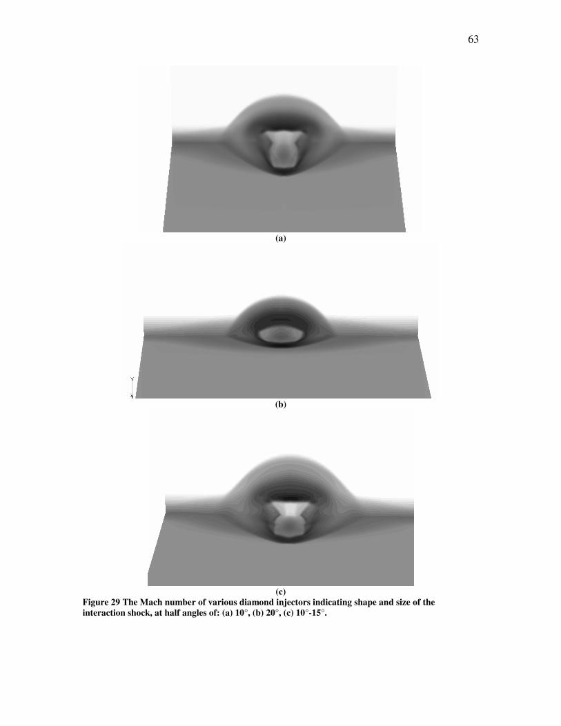
63

(a)

(b)

(c)

Figure 29 The Mach number of various diamond injectors indicating shape and size of the interaction shock, at half angles of: (a) 10°, (b) 20°, (c) 10°-15°.

64

(a) (b)

(c) (d) Figure 30 The vortex cores of various diamond injector, with the following half angles: (a) 15°, (b) 10°, (c) 20°, (d) 10°-15°.

65

(a) (b)

(c) (d) Figure 31 The boundary layer interaction with the horseshoe vortex in front of different diamond injectors, with the following half angles: (a) 15°, (b) 10°, (c) 20°, (d) 10°-15°.

66

(a)

(b)

(c)

Figure 32 The shadow graph of various diamond injectors, at half angles of: (a) 10°, (b) 20°, (c) 10°-15°.

67

(a)

(b)

(c)

Figure 33 The dual 15° injector Mach numbers displayed at the following distances downstream from the center of the diamond injector: (a) x/d = 0, (b) x/d = 2, (c) x/d =5.

68

(a)

(b)

(d)

Figure 34 The dual 10° injector Mach numbers displayed at the following distances downstream from the center of the diamond injector: (a) x/d = 0, (b) x/d = 2, (c) x/d = 5.

69

APPENDIX C

DIAMOND INJECTORS IN MACH 2 FREESTREAM

In order to further expand the database for diamond injectors. Two additional cases

were performed for diamond injectors with half angles of 10° and 15° at a freestream of

Mach 2. Each CFD case performed was investigated for the transverse counter rotating

vortex pair, as found in the 15° half angle case Srinivasan and Bowersox18 originally

studied described in Chapter II. This case serves as the baseline for the present

discussion.

C.1 10° Half Angle

The 10° half angle injector developed the same barrel shock at Mach 2 as the 15°

baseline at Mach 5. The trailing edge formed a flat “V” shaped plane. The transverse

counter rotating vortex pair formed at the trailing edge of the injector.

C.2 15° Half Angle

The 15° half angle injector developed the same barrel shock at Mach 2 as the 15°

baseline. The barrel shock created the flat “V” shape at the trailing edge, similar to all the

cases containing the TCVP. The TCVP does form at the trailing edge of the diamond

injector.

70

APPENDIX D

ADDITIONAL FIGURES

(a) (b)

(c) (d)

Figure 35 Barrel shock formation of various diamond injectors, at the following half angles: (a) the leading edge of a 10° half angle, (b) the trailing edge of a 10° half angle, (c) the leading edge of a 15° half angle, (d) the trailing edge of a 15° half angle.

71

(a)

(b)

Figure 36 Transverse counter rotating vortex pair formation at the trailing edge of the following diamond injectors: (a) 10°, (b) 15°.

72

VITA

Justin Walter McLellan received his Bachelor of Science degree in aerospace

engineering from The State University of New York at Buffalo in 2003. He entered the

Aerospace Engineering program at Texas A&M University in September 2003, where he

received his Master of Science degree in August 2005. His research interests include

computational fluid dynamics in both compressible and incompressible flow, specifically

diamond injector performances as fuel injectors for scramjet propulsion. He will be

publishing a paper on jet in supersonic crossflow interaction through the American

Institute of Aeronautics and Astronautics journal this December.

Mr. McLellan may be reached at SAIC, 2111 Eisenhower, Suite 303, Alexandria, VA

22314. His email address is jwmclellan@gmail.com.