The Effects of Default Risk and Liquidity Risk on Implied Cost of Capital

Yang Yang

yyang44@tigers.lsu.edu

Louisiana State University

Department of Finance

Abstract

It has been common knowledge that liquidity risk and default risk play a role in a firm’s cost of equity

capital. However, two latent issues have yet to be solved: 1. What’s the relative importance of default and

liquidity effects in equity return? 2. Is realized stock return a good proxy for cost of equity capital on the

left hand side? This paper uses implied cost of capital (ICC) to proxy for stock returns and examines the

two risks together. I find that, while default risk still plays the major role in general, the contribution of

liquidity risk varies among different proxies of expected returns. I use the approaches in Hou et al (2012)

to estimate ICC. I model liquidity measures using the method developed in Amihud (2002) and Liu

(2006). Merton (1974), Bharath and Shumway (2004), and Vassalou and Xing (2004) give the guideline

to estimate default measure.

1. Introduction

It seems to be a tradition that ex post realized stock returns have been used to estimate firm’s expected

stock return (or cost of equity capital), and further studies have revealed the relation between firm

characteristics and expected returns. However, realized stock returns are ex post whereas expected stock

returns are ex ante. Moreover, many researchers have proved that realized returns are a noisy proxy for

expected returns.

Recent accounting and finance studies including Gordon and Gordon, 1997; Claus and Thomas, 2001;

Gebhardt et al., 2001; Easton, 2004; and Ohlson and Juetttner-Nauroth, 2005 have proposed an alternative

approach to estimate expected returns: the implied cost of Capital (ICC). The ICC of a firm is the internal

rate of return that equates the firm’s stock price to the present value of expected future cash flows. In

other words, the ICC is the discount rate that the market uses to discount the expected cash flows of the

firm. The main advantage of the ICC is that it’s much less noisy than realized returns and it does not rely

on any specific asset pricing model. The estimation of ICC only requires stock prices and cash flow

forecasts.

There are two most common approaches in estimating ICC literatures: Analyst forecast based models and

Regression based models. The former uses analysts’ earnings forecasts to proxy for cash flow

expectations. The latter uses regression based on historical accounting data to generate/predict future

earnings. However, recent empirical papers have provided evidence that analyst-based ICC doesn’t have

superior predictive power on realized returns. Furthermore, a large body of research (Francis and

Philbrick, 1993; Dugar and Nathan, 1995; McNichols and O’Brien, 1997; Lin and McNichols. 1998)

documents that analysts tend to be overly optimistic in their forecasts. Another concern is the IBES

analyst data are only available after the late 1970s and small firms and financially distressed firms are

underrepresented. As a result, the analyst-based ICC has limited both cross-sectional and time-series

coverage. In this paper, I use analyst-based ICC first because of quicker data generating process. I also

include model based ICC. The advantage of the model-based approach is that it’s not limited by the small

population covered by IBES. The first records can be traced to as early as 1968 and small and distressed

firms are not lost. The larger sample size will improve the robustness of the model and the estimating

results.

Liquidity risk has been proved to be a risk factor in expected stock returns. There are, however, numerous

ways to model liquidity risk. One prominent measure is constructed by Pastor and Stambaugh (2003), in

which paper they find significant cross-sectional relation between expected stock returns and the

sensitivities of returns to fluctuations in aggregate liquidity. Another important measure of liquidity risk is

constructed by Liu (2006), where he finds a two-factor (market and liquidity) model well explains the

cross-section of stock returns. In this paper I adopt the methodology proposed in Liu (2006) to measure

liquidity risk because this measure highlights four dimensions to liquidity: trading quantity, trading speed,

trading cost and price impact. This method should serve as a more comprehensive measure of liquidity

risk compared to the measure constructed by Pastor and Stambaugh (2003). I also separate NASDAQ

stocks from the NYSE/AMEX/NASDAQ stock universe because NASDAQ stocks (liquidity) are inflated

relative to NYSE/AMEX stocks due to interdealer trades.

Until last decade, one of the most common proxies for default risk is default spread. The default spread is

usually defined as the yield or return differential between long-term BAA corporate bonds and long-term

AAA or U.S. Treasury bonds. Elton et al. (2001), however, shows that much of the information in the

default spread is unrelated to default risk. The most referenced option pricing model to compute default

measures is Merton’s (1974) option pricing model. The first study that uses Merton (1974) option pricing

model to compute default measures for individual firms and assess the effect of default risk on equity

returns is Vassalou and Xing (2004). By modeling default risk using Merton’s model, Vassalou and Xing

(2004) finds that default risk is intimately related to the size and book-to-market (BM) characteristics of a

firm. They conclude that both the size and BM effects can be viewed as default effects. They also find

that, under some conditions, high-default-risk firms earn higher returns than low default risk firms and

they further examine that default risk is a systematic risk.

As discussed in Vassalou and Xing (2004), one major concern of using accounting models in estimating

the default risk of equities are accounting information are derived from firm’s financial statements which

are inherently backward looking. An alternative source of information for calculating default risk

measures is the bonds market. However, a key assumption of using bond rating history is that all assets

within a rating category share the same default risk and that this default risk is equal to the historical

average default risk, thus a firm can’t experience a change in its default probability without experiencing

a rating change. In real life, typically, the change in the probability of default is observed with a lag, and

usually bond rating agencies tend to be very reluctant to adjust ratings upward.

Vassalou, Chen and Zhou (2006) suggests that the inclusion of default and liquidity variables in popular

asset pricing specifications improves a model’s performance and the improvement is much larger when

the included variable is default, rather than liquidity. This paper, however, finds that the contribution of

liquidity risk varies among different proxies of expected returns, for example, implied cost of capital.

While default effect is still a higher order effect than liquidity in general, using single proxy of expected

stock return is not a safe way to reach the conclusion that default risk dominates liquidity risk or the other

way around. Furthermore, different measures of implied cost of capital may contain different information

that may have different weights between default risk and liquidity risk by nature. This also suggests that

the refinement of existing ICC measures may be necessary. Implied cost of capital is the discount rate that

equates the firm’s stock price to the present value of expected future cash flows. Implied cost of capital is

an internal rate of return by formula. Default risk playing the major role in implied cost of capital (in

general) suggests that it is a more persistent risk than liquidity risk.

The remainder of the paper is organized as follows. Section 2 introduces the data and the sample selection.

Section 3 discusses the estimation of the ICC. Section 4 estimates firm’s default risk using Merton’s

model and Vassalou and Xing’s approach. Section 5 estimates liquidity measures using Illiquidity ratio by

Amihud (2002) and liquidity measure (LM12) in Liu (2005). Section 6 discusses the relation between a

firm’s ICC and the two risks. I conclude in Section 7 with a summary of my results.

2. Data and sample selection

To be consistent with Hou et al. (2012), my sample includes all NYSE, Amex, and Nasdaq listed

securities with sharecodes 10 or 11 (i.e., excluding ADEs, closed-end funds, and REITs) that are at the

intersection of the CRSP monthly returns file from July 1963 to June 2012, the Compustat fundamentals

annual file from 1963 to 2012 and IBES earning forcast from 1975 to 2012. Variable definitions are as

follows. Earning is income before extraordinary items from Compustat. Book equity is Compustat

stockholder’s equity. Total assets and dividends are also from Compustat. Prior to 1988, accruals are

calculated using the balance sheet method as the change in non-cash current assets less the change in

current liabilities excluding the change in short-term debt and the change in taxes payable minus

depreciation and amortization expense. Starting in 1988, I use the cash flow statement method to calculate

accruals as the difference between earnings and cash flows from operations.

3. Estimation of ICC

In this paper, I adopt three ways to construct ICC: 1. Analysts based approach; 2. Regression based

approach; 3. Price Multiple (Naïve) approach. In the end, I also generate predicted stock returns based on

Fama French three factor model. Table 1 reports the summary statistics of all the ICC measures, including

predict stock return.

[Table 1. Summery Statistics of Various Measures of ICC and predicted stock returns]

3.1. Analysts based cross-sectional earnings model

I use analysts’ forecasts of earnings per share to proxy for cash flow expectations. I estimate analysts-

based earnings forecasts for up to 3 years into the future and then use those earnings forecasts to compute

the ICC for all the firm-year observations covered by both COMPUSTAT and CRSP. I scale the

regression-based earnings forecasts using a firm’s end-of-June market equity and analysts’ per share

earnings forecasts using the end-of-June stock price to report them all in the same units. All earnings and

growth rate data are from IBES database.

Having the forecasted earnings, ICC can be estimated. In this paper ICC is calculated using MPEG

method in Easton (2004).

𝑀𝑡 =Et[Et+2]+R∗Et[Dt+1]−Et[Et+1]

R2 (1)

Where Mt is the market equity in year t,

R is the implied cost of capital (ICC),

Et[ ] denotes market expectations based on information available in year t. Et+1 and Et+2 are the

earnings in years t+1 and t+2, respectively.

Dt+1 is the dividend in year t+1, computed using the current dividend payout ratio for firms with

positive earnings. If a firm has negative earnings, the current dividend payout ratio is estimated by

(current dividends) / (0.06 * total assets). Every month IBES updates analysts’ forecasts, so that ICC can

be computed on monthly basis.

The summery statistics and correlations between all measures of ICC can be found in Table 1. Analysts

based ICC has an average of 10.3% for NYSE and AMEX stocks, and 11.9% for NASDAQ stocks. The

correlation between analysts based ICC and regression based ICC is 0.30 for NYSE and AMEX stocks,

and 0.05 for NASDAQ stocks. The correlation between analysts based ICC and price multiple ICC is 0.13

for NYSE and AMEX stocks, and 0.16 for NASDAQ stocks. The correlation between analysts based ICC

and predicted stock return is very marginal for all the stocks.

3.2 Regression based cross-sectional earnings model

For each year between 1975 and 2012, I estimate the following pooled cross-sectional regressions using

the previous ten years of data:

Ei,t+τ = α0 + α1Ai,t + α2Di,t + α3DDi.t + α4Ei,t + α5NegEi,t + α6ACi,t + εi,t+ τ, (2)

Where Ei,t+τ is forecast earnings of firm i in year t + τ (τ = 1 to 3),

Ai,t is the total assets,

Di,t is the dividend payment,

DDi.t is a dummy variable that equals 1 for dividend papers and 0 otherwise,

NegEi,t is a dummy cariable that equals 1 for firms having negative earnings and 0 otherwise,

ACi,t is accruals. Before 1982, Accruals are calculated by balance sheet method; after 1982 they

are calculated by cash flow method.

The variables on the right hand side are based on a combination of the cross-sectional profitability models

in Fama and French (2000, 2006), Hou and Robinson (2006), and Hou and van Dijk (2011). All

explanatory variables are measured as of year t.

Every month I compute the regression-based earning forecast for subsequent three future years by

applying historically estimated coefficients from equation (2) to the most recent set of publicly available

accounting data. This is to ensure that the earnings forecasts are strictly out of sample. In addition, the

survivorship bias is kept to a minimum because earnings forecasts can be estimated by simple firm

characteristics. After constructing the regression-based earnings forecasts for subsequent three future

years (Ei,t+1, Ei,t+2, and Ei,t+3), I calculate the long-term growth rates for individual firms as Ltg = (Ei,t+3

/Ei,t+2 + Ei,t+2 /Ei,t+1)/2 -1. Regression-based ICC can be calculated then by applying equation (1).

The summery statistics and correlations between all measures of ICC can be found in Table 1. Regression

based ICC has an average of 3.28% for NYSE and AMEX stocks, and 3.16% for NASDAQ stocks. The

correlation between regression based ICC and price multiple ICC is 0.03 for NYSE and AMEX stocks,

and 0.004 for NASDAQ stocks. The correlation between regression based ICC and predicted stock return

ICC is marginal for all the stocks.

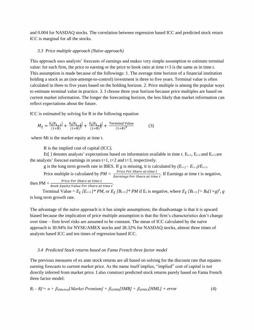
3.3 Price multiple approach (Naïve approach)

This approach uses analysts’ forecasts of earnings and makes very simple assumption to estimate terminal

value: for each firm, the price to earning or the price to book ratio at time t+3 is the same as in time t.

This assumption is made because of the followings: 1. The average time horizon of a financial institution

holding a stock as an (not-attempt-to-control) investment is three to five years. Terminal value is often

calculated in three to five years based on the holding horizon. 2. Price multiple is among the popular ways

to estimate terminal value in practice. 3. I choose three year horizon because price multiples are based on

current market information. The longer the forecasting horizon, the less likely that market information can

reflect expectations about the future.

ICC is estimated by solving for R in the following equation

𝑀𝑡 =Et[Et+1]

(1+R)+

Et[Et+2]

(1+R)2 + Et[Et+3]

(1+R)3 + Terminal Value

(1+R)3 (3)

where Mt is the market equity at time t.

R is the implied cost of capital (ICC).

Et[ ] denotes analysts’ expectations based on information available in time t. Et+1, Et+2 and Et+3 are

the analysts’ forecast earnings in years t+1, t+2 and t+3, respectively.

g is the long term growth rate in IBES. If g is missing, it is calculated by (Et+2 – Et+1)/Et+1.

Price multiple is calculated by PM = 𝑃𝑟𝑖𝑐𝑒 𝑃𝑒𝑟 𝑆ℎ𝑎𝑟𝑒 𝑎𝑡 𝑡𝑖𝑚𝑒 𝑡

𝐸𝑎𝑟𝑛𝑖𝑛𝑔𝑠 𝑃𝑒𝑟 𝑆ℎ𝑎𝑟𝑒 𝑎𝑡 𝑡𝑖𝑚𝑒 𝑡. If Earnings at time t is negative,

then PM = 𝑃𝑟𝑖𝑐𝑒 𝑃𝑒𝑟 𝑆ℎ𝑎𝑟𝑒 𝑎𝑡 𝑡𝑖𝑚𝑒 𝑡

𝐵𝑜𝑜𝑘 𝐸𝑞𝑢𝑖𝑡𝑦 𝑉𝑎𝑙𝑢𝑒 𝑃𝑒𝑟 𝑆ℎ𝑎𝑟𝑒 𝑎𝑡 𝑡𝑖𝑚𝑒 𝑡.

Terminal Value = 𝐸𝑡 [Et+3 ]* PM, or 𝐸𝑡 [Bt+3 ]* PM if Et is negative, where 𝐸𝑡 [Bt+3 ]= B0(1+g)3, g

is long term growth rate.

The advantage of the naïve approach is it has simple assumptions; the disadvantage is that it is upward

biased because the implication of price multiple assumption is that the firm’s characteristics don’t change

over time – firm level risks are assumed to be constant. The mean of ICC calculated by the naïve

approach is 30.94% for NYSE/AMEX stocks and 38.32% for NASDAQ stocks, almost three times of

analysts based ICC and ten times of regression based ICC.

3.4 Predicted Stock returns based on Fama French three factor model

The previous measures of ex ante stock returns are all based on solving for the discount rate that equates

earning forecasts to current market price. As the name itself implies, “implied” cost of capital is not

directly inferred from market price. I also construct predicted stock returns purely based on Fama French

three factor model:

Ri – Rf = α + βi(Market)[Market Premium] + βi(SMB)[SMB] + βi(HML)[HML] + error (4)

Where Ri is a firm’s stock return at time t.

Rft is risk-free interest rate (one month Treasury bill rate).

Market Premium is the excess return on the market. It is calculated as the value-weight return on all

NYSE, AMEX, and NASDAQ stocks minus the one-month Treasury bill rate.

SMB (Small Minus Big) is the average return on the three small portfolios minus the average return

on the three big portfolios.

HML (High Minus Low) is the average return on the two value portfolios minus the average returns

on the two growth portfolios.

βi Is the Fama-French factor.

All the risk premium data and risk free rate are from WRDS Fama French factors database. This data can

also be found on Kenneth French’s website at Dartmouth.edu.

I first run pooled regressions on 12 consecutive monthly data of a firm and generate the firm specific

coefficients (βs). Then I multiply the generated coefficients by according risk premiums in the 13th month

on the right hand side. After adding risk free rate, I get the predicted (firm specific) stock returns based on

the past 12 months. The mean predicted stock return is 1.37% for NYSE/AMEX stocks, and 2.09% for

NASDAQ stocks. The correlations between predicted stock return and all the measures of ICC are

relatively marginal. In whatever measures, the average ICC of NASDAQ stocks are higher than that of

NYSE/AMEX stocks.

3.4 The appropriate proxy of ex ante expected stock return

Generally speaking, the higher a project’s internal rate of return, the more desirable it is to undertake the

project. Internal rate of return can also been viewed as the rate of growth a project is expected to generate.

Internal rate of return can be compared against prevailing rates of return in the securities market. Ideally

ICC (or IRR) shouldn’t be lower than (stock) market return. If a firm can’t find any projects with internal

rate of returns greater than the returns that can be generated in the financial markets, it may simply choose

to invest its retained earnings into the market. Firms shouldn’t adopt projects whose IRR is even lower

than the percentage change of gross domestic product (GDP). Gross domestic product (GDP), the featured

measure of U.S. output, is the market value of the goods and services produced by labor and property

located in the United States. Table 2 reports the annual means of all measures of ICC, predict stock

returns and the U.S. GDP growth rate. Figure 1 and Figure 2 plot the trends of all measures of ICC

including predict stock returns and GDP annual growth rate over 1982 to 2012 period. In the three

measures of ICC above, analysts based ICC and price multiple based ICC are significantly higher than

annual percentage change of GDP. Regression based ICC is very stable, but is lower than the annual

percentage change of GDP. I treat NYSE/AMEX and NASDAQ stocks as different sample, because the

liquidity measure is twisted in NASDAQ stocks and will be discussed later in section 5. GDP data can be

found on Federal Reserve Bank of St. Louis website. Regression based ICC is apparently too low and

price multiple based ICC seems to be too high. Analysts’ based ICC shares the similar trend as GDP, yet

it is less volatile than price multiple based ICC.

[Table 2. Annual Means of All Measures of ICC, Predict Stock Returns and The U.S. GDP Growth

Rate]

[Figure 1] Trends of Implied Cost of Capital for NYSE/AMEX stocks

[Figure 2] Trends of Implied Cost of Capital for NASDAQ stocks

-0.05

0

0.05

0.1

0.15

0.2

0.25

0.3

0.35

0.4

ICC Trends (NYSE/AMEX)

Analysts Based ICC

Regression Based ICC

Price Multiple ICC

Predicted Stock Returns

GDP annual pctg change

-0.1

0

0.1

0.2

0.3

0.4

0.5

0.6

ICC Trends (NASDAQ)

Analysts Based ICC

Regression Based ICC

Price Multiple ICC

Predicted Stock Returns

GDP annual pctg change

4. Estimation of firm’s default risk

Forecasting corporate defaults has always been an interesting topic in both practice and academic. Default

risk is the uncertainty of a firm’s ability to service its debts and obligations. Before the first application of

Merton’s model in Vassalou and Xing (2004), default risk was usually measured by default spread. The

argument is that lenders require different premiums to compensate different level of risk in case of default.

Fama and Schwert (1977), Keim and Stambaugh (1986), Campbell (1987), and Fama and French (1989)

have shown that the yield spread between investment grade and non-investment grade corporate bond can

predict expected returns in stocks and bonds. However, Elton et al. (2001) finds that default spread is a

noisy measure in the sense that it contains too much information that is unrelated to default risk and is

hard to distangle.

Default seems to be a rare event. The probability of a firm that actually ends up into default is only

around 2% in any year. However, there is considerable variation in default probabilities across firms.

Furthermore, for two firms with an identical default probability, the loss in the event of default (loss given

default) can vary widely depending on their nature (security, collateral, seniority, etc.). Credit risk can be

categorized into two groups: 1. Standalone Risk. 2. Portfolio Risk. The first category includes three types

of risk: default probability, loss given default, migration risk. Migration risk is the probability and value

impact of changes in default probability. The second category includes two types of risk: default

correlations, and exposure. The default correlations measure the degree to which the default risks of the

borrowers and counterparties in the portfolio that are related. The exposure is the size, or proportion, of

the portfolio exposed to the default risk of each counterparty and borrower. Due to the focus of the study

and the limitation of database, this paper only concentrates on default risk measured by default probability.

The other types of credit risk are not studied here.

Today the most widely applied default probability forecasting model is a particular application of

Merton’s model (Merton, 1974) that was developed by the KMV Corporation, which is referred to the

KMV-Merton model here. The first papers discussed Merton’s model are Saunders and Allen (2002) and

Duffie and Singleton (2003). Application of the model in Vassalou and Xing (2004) made it well known

and widely accepted in practice. The KMV-Merton model is a no trivial development of Merton’s model,

so the full name, as referred in Bharath and Shumway (2004), is referred to the same here. The complete

KMV-Merton model uses a more complicated method to assess the asset volatility, which incorporates

Bayesian adjustments for the country, industry, and size of the firm. It also allows for convertibles and

preferred stocks in the capital structure of the firm. Due to limited database, however, neither Vassalou

and Xing (2004) or Bharath and Shumway (2004) could adopt the full model. Because of database

limitations, the default measure came up in their paper are given different names to indicate that it is not

the exact default probabilities derived from KMV-Merton model, even though the procedure is almost the

same. Vassalou and Xing (2004) calls it Default Likelyhood Indicators (DLI), and Bharath and Shumway

(2004) calls it Expected Default Frequency (EDF). In this paper, due to the same reason in the two papers

mentioned above, I replicate Bharath and Shumway (2004)’s procedure to construct EDF.

4.1 The KMV-Merton Model

Equity holders have residual claims on a firm’s assets after all other obligations have been met, thus the

equity of a firm can be seen as a call option on the firm’s assets. The strike price of the call option is the

book value of the firm’s liabilities. The equity is of no value if the value of the firm’s assets is less than

the strike price, i.e., the book value of the firm’s liabilities.

The KMV-Merton default forecasting model generates a probability of default for each firm at any given

point of time. The two major steps in very simple terms are: 1. Calculate a z-score, which is often referred

to as the distance to default. 2. Substitute the z-score (or distance to default) into a cumulative density

function to calculate the default probability. In the first step, the model subtracts the face value of the

firm’s debt from an estimate of the market value of the firm and then divides this difference by an

estimate of the volatility of the firm (scaled to reflect the horizon of the forecast). The default probability

is defined as the probability that the value of the firm is less than the face value of debt at the forecasting

horizon.

Market value of debt is a crucial input in KMV-Merton model, however unlike market value of equity,

market value of debt is not easy to observe in public market. The KMV-Merton model estimates the

market value of debt by applying the Merton (1974) bond pricing model. Except a few others, there are

two particularly important assumptions in Merton model. The first is that the total value of a firm is

assumed to follow geometric Brownian motion,

𝑑𝑉 = 𝜇𝑉𝑑𝑡 + 𝜎𝑉𝑉𝑑𝑊 (5)

Where V is the total value of the firm, µ is the expected continuously compounded return on V, σV is the

volatility of firm value and dW is a standard Weiner process. The second important assumption of the

Merton model is that the firm has issued just one discount bond maturing in T periods. With all the

assumptions and by put-call parity, the equity value of a firm can be expressed as

𝐸 = 𝑉𝑁(𝑑1) − 𝑒−𝑟𝑇𝐹𝑁(𝑑2), (6)

where E is the market value of the firm’s equity, F is the face value of the firm’s debt, r is the

instantaneous risk-free rate, N(·) is the cumulative standard normal distribution function, d1 is given by

𝑑1 = ln(𝑉 𝐹⁄ )+(𝑟+0.5𝜎𝑉

2)𝑇

𝜎𝑉√𝑇, (7)

and

𝑑2 = 𝑑1 − 𝜎𝑉√𝑇, (8)

The rationale behind the expressions above is that the value of the firm’s debt is equal to the value of a

risk-free discount bond minus the value of a put option written on the firm, again with a strike price equal

to the face value of debt and a time-to-maturity of T.

In the KMV-Merton model, E (total value of the firm’s equity) is easy to observe by multiplying the

firm’s current stock price by its shares outstanding, but V (the total value of the firm) must be inferred. In

that sense, the volatility of equity, σE can be estimated but σV, the volatility of the firm, must be inferred

too. Following Bharath and Shumway (2004), I adopt an iterative procedure to calculate σV. I use daily

data from the past 12 months to obtain an estimate of the volatility of equity σE, which is then used as an

input in σV = σE [ E / ( E + F ) ]. The resulting σV would be the input of equation (6). Then I can

compute V for each trading day of the past 12 months based on the E of that day. With the daily (trading

day) estimation of V, I can estimate the standard deviation of V, which is used as the value of σV, for the

next iteration. This procedure is repeated until the values of σV from two consecutive iterations converge.

The tolerance level for convergence is 10E-3. It takes only a few iterations for σV to converge. Once the

converged value of σV is obtained, I use it to back out V through equation (7). This process is repeated at

the end of every month, so I will have monthly values of σV. The risk-free rate used for the process is

monthly annualized yield calculated from nominal price (KYTREASNOX) in CRSP treasuries monthly

time series database.

Once σV and σ are calculated, the distance to default (DD) can be calculated as

𝐷𝐷 = ln(𝑉 𝐹⁄ )+(𝜇−0.5𝜎𝑉

2)𝑇)

𝜎𝑉√𝑇, (9)

where µ is an estimate of the expected annual return of the firm’s assets. Equation (9) can be seen as a z-

score. Based on z-score, we can find corresponding implied probability of default, sometimes called the

expected default frequency (or EDF), to be

𝐸𝐷𝐹 = 𝜋𝐾𝑀𝑉 = 𝑁 (− (ln(𝑉 𝐹⁄ )+(𝜇−0.5𝜎𝑉

2)𝑇)

𝜎𝑉√𝑇)) = 𝑁(−𝐷𝐷). (10)

4.2 Data

The sample includes all firms in the intersection of the Compustat Industrial file – Quarterly data and

CRSP daily stock return for NYSE, AMEX and NASDAQ stocks between 1960 and 2012. Financial

firms are excluded. The risk-free rate is monthly annualized yield calculated from nominal price

(KYTREASNOX) in CRSP treasuries monthly time series database. E is calculated from CRSP as the

product of share price at the end of the month and the number of shares outstanding. Consistent with

Vassalou and Xing (2003), F, the face value of debt, is debt in current liabilities (DLCQ in Compustat)

plus one half of long term debt (DLTTQ in Compustat). Following Shumway (2001) and Bharath and

Shumway (2004), I measure each firm’s past excess return in year t as the return of the firm in year t-1

minus the value-weighted CRSP NYSE/AMEX index return in year t-1 (rit-1 – rmt-1). Each firm’s annual

returns are calculated by cumulating monthly returns. The observations are winsorized on 1% level. The

resulting EDF is a monthly measure. Table 3 Panel A gives the summary statistics of monthly estimation

of EDFs. Table 3 Panel B reports the annual means of EDF from 1982 to 2012. Figure 3 plots the overall

trend according to Table 3 Panel B. Interestingly, the overall expected default frequency of NASDAQ

stocks is higher than that of NYSE/AMEX stocks.

[Table 3] Summary Statistics of Expected Default Frequency and Annual Means of EDF

Panel A: Summary Statistics of EDF

NYSE/AMEX Nasdaq

OBS 201181 155401

Mean 14.92% 18.52%

Std.Dev. 28.69% 30.92%

Median 0.08% 0.50%

Panel B: Annual Means of EDF

year NYSE/AMEX Nasdaq

1982 29.71% 20.32%

1983 5.44% 6.99%

1984 13.99% 22.37%

1985 9.02% 15.90%

1986 6.17% 13.06%

1987 10.41% 19.51%

1988 21.77% 31.10%

1989 10.20% 14.89%

1990 23.64% 27.58%

1991 16.09% 23.29%

1992 10.21% 15.56%

1993 8.83% 13.85%

1994 14.72% 14.49%

1995 13.95% 16.22%

1996 11.54% 17.39%

1997 11.28% 15.71%

1998 17.27% 21.25%

1999 29.29% 31.58%

2000 34.72% 29.90%

2001 21.24% 28.96%

2002 16.72% 18.22%

2003 15.59% 17.23%

2004 5.47% 5.62%

2005 10.07% 14.32%

2006 9.14% 12.40%

2007 8.42% 15.35%

2008 20.92% 29.79%

2009 31.44% 31.12%

2010 4.99% 8.29%

2011 5.29% 6.96%

2012 10.86% 10.98%

[Figure 3] Annual Means of Expected Default Frequency

5. Estimation of Market Liquidity

Liquidity is a broad concept that generally denotes the ability to trade large quantities quickly, at low cost,

and without moving the price. There are three dimensions of liquidity: security level, market level and

financial institution level. In terms of security, liquidity denotes the ease with which the security can be at

low cost and even in large amounts on a secondary market. In terms of market, it denotes the liquidity of

the securities traded in the market, measured by proxies such as volume and bid-ask spread etc. In terms

of financial institution, liquidity denotes the ability to fund increases in assets and meet obligations as

they come due, without incurring high losses. The difference between the liquidity of assets and that of

liabilities is a general proxy.

There are two types of liquidity risk. The first is funding risk, a risk that a financial institution may not be

able to face efficiently any expected or unexpected cash outflows. The second is market liquidity risk, a

risk that the liquidation of a sizable amount of assets will have great (negative) impact on market price.

The two types of risk are connected, however, this paper focuses on market liquidity risk.

To accurately measure market liquidity, four dimensions should be simultaneously taken into

consideration: trading quantity, trading speed, trading cost, and price impact. The bid-ask spread measure

in Amihud and Mendelson (1986) relates to the trading cost dimension, the turnover measure of Datar et

al (1998) relates to the trading quantity dimension. The later widely accepted liquidity measures in

Amihud (2002) and Pastor and Stambaugh (2003) incorporate price impact. Pastor and Stambugh also

provides empirical evidence that market wide liquidity is a state variable important for asset pricing.

Finally Liu (2006) integrates all the four dimensions (including trading speed) into one liquidity measure

and shows that (market) liquidity is an important source of priced risk. Liu (2006) also finds a two-factor

(market and liquidity) model well explains the cross-section of stock returns, describing the liquidity

0

0.05

0.1

0.15

0.2

0.25

0.3

0.35

0.4

1982198419861988199019921994199619982000200220042006200820102012

Annual Means of Expected Default Frequency

NYSE/AMEX

Nasdaq

premium, subsuming documented anomalies associated with size, long-term contrarian investment, and

fundamental (cashflow, earnings, and dividend) to price ratios. In particular, his two-factor model

accounts for the book-to-market effect, which the Fama-French three-factor model fails to explain. Given

the nature of liquidity, one single measure is unlikely to adequately capture or describe all the dimensions

it may have. For this reason, I employ two alternative liquidity measures. They are Amihud’s (2002)

illiquidity ratio and and Liu’s liquidity measure (LM12).

My results show that the two alternative liquidity measures are very marginally correlated with each other

(negatively), which suggest that either one of them captures different information.

5.1 Amihud (2002) Illiquidity Measure

Amihud (2002) suggests that expected stock excess return partly represents an illiquidity premium, by

showing that expected market illiquidity positively affects ex ante stock excess return over time. He

defines stock illiquidity as the average ratio of the daily absolute returns to the (dollar) trading volume on

that day, │Riyd│/VOLDiyd. Riyd is the return on stock i on day d of year y and VOLDiyd is the respective

daily volume in dollars. The rationale behind the illiquidity measure is Kyle’s concept of illiquidity - the

response of price to order flow – and Silber’s (1975) measure of thinness. The details can be found in

Amihud (2002).

In order to make all the variables consistent in the same frequency (which is monthly), the cross-sectional

study employs for each stock i the monthly average

𝐼𝐿𝐿𝐼𝑄𝑖𝑦𝑚 = 1/𝐷𝑖𝑚 ∑|𝑅𝑖𝑚𝑑|

𝑉𝑂𝐿𝐷𝑖𝑣𝑚𝑑,𝐷𝑖𝑚𝑡=1 (11)

where Dim is the number of days for which data are available for stock i in year y and month t. Table 4

reports the summary statistics of both measures of liquidity (illiquidity).

5.2 Liu (2006) liquidity measure

This paper follows Liu (2006)’s way of constructing liquidity measure. The liquidity measure of a

security, LMx, as the standardized turnover-adjusted number of zero daily trading volumes over the prior

x months ( x = 1, 6, 12), that is,

𝐿𝑀𝑥 = [ 𝑁𝑢𝑚𝑏𝑒𝑟 𝑜𝑓 𝑧𝑒𝑟𝑜 𝑑𝑎𝑖𝑙𝑦 𝑣𝑜𝑙𝑢𝑚𝑒𝑠 𝑖𝑛 𝑝𝑟𝑖𝑜𝑟 𝑥 𝑚𝑜𝑛𝑡ℎ𝑠 + 1

𝑥 𝑚𝑜𝑛𝑡ℎ 𝑡𝑢𝑟𝑛𝑜𝑣𝑒𝑟

𝐷𝑒𝑓𝑙𝑎𝑡𝑜𝑟] ∗ 21𝑥/𝑁𝑜𝑇𝐷 (12)

where x-month turnover is turnover over the prior x months, calculated as the sum of daily turnover over

the prior x periods, daily turnover is the ratio of the number of shares traded on a day to the number of

shares outstanding at the end of the day, NoTD is the total number of trading days in the market over the

prior x months, and Deflator is chosen such that

0 <

1𝑥 𝑚𝑜𝑛𝑡ℎ 𝑡𝑢𝑟𝑛𝑜𝑣𝑒𝑟

𝐷𝑒𝑓𝑙𝑎𝑡𝑜𝑟< 1

for all sample stocks. Following Liu (2006), I use a deflator of 11,000 in constructing LM12.

Equation (12) contains necessary information from all four dimensions of market liquidity, emphasizing

particularly on trading speed. For the same reason argued in Liu (2006) that both LM1 and LM6 fail to

distinguish some illiquid securities in NASDAQ ordinary common stocks, I adopt LM12 as the liquidity

measure in this paper, that is LMx = LM12. Because all the variables are to be controlled within the same

frequency, I aggregate (daily) LM12 on monthly level: summation of the past one month LM12s. In order

to differentiate from the original LM12 in Liu (2006), the summation of the past 1-month LM12 is called

LM12M.

5.3 Data

The sample comprises all NYSE/AMEX/NASDAQ ordinary common stocks over the period January

1960 to December 2012. Because market makers inflate the trading volumes for NASDAQ stocks, the

liquidity effect is examined separately for NYSE/AMEX stocks and NASDAQ stocks. All the necessary

data are from CRSP daily data. Because trading volumes for NASDAQ stocks are inflated relative to

NYSE/AMEX stocks due to interdealer trades, I examine the liquidity measure (and other measures in

this paper) separately for NYSE/AMEX stocks and NASDAQ stocks. Table 4 Panel A gives the

summary statistics of daily measure of LM12M. Panel B gives the correlations between the two measures.

Table 5 reports the annual means of illiquidity ratio and LM12M from 1982 to 2012 for both

NYSE/AMEX and NASDAQ stocks. I exclude the first two years of NASDAQ LM12M because they

were too large compared to later averages (also suggesting that NASDAQ stocks were very illiquid at the

time when NASDAQ just entered the business). The average LM12M of NASDAQ stocks is 7310.6 and

3895.2 in 1982 and 1983, respectively. Since 1984, the average LM12M has dropped down gradually,

compared to the drastic change in 1982 and 1983. The correlation between the two measures being

negative is as expected: larger LM12M means worse liquidity whereas larger Amihud (2002) ratio means

better liquidity. Figure 4 and Figure 5 plot the trend of annual means of liquidity measures from 1982 to

2012.

5.4 Default risk and Liquidity (Illiquidity) measure

Many literatures have found that default risk is associated with equity returns and so is liquidity risk. One

would expect default risk and liquidity risk to be interrelated. Vassalou, Chen and Zhou (2006) uses three

liquidity measures (except Liu (2006)’s measure) and default probability based on Merton’s (1974). They

find that, consistent with previous literatures, the inclusion of default and liquidity variables in popular

asset pricing specifications improves a model’s performance. However, improvement is much larger

when the included variable is default rather than liquidity. The robustness of these relations remains

unaltered when they take into account the correlation of the default and liquidity measures with aggregate

stock market volatility.

Table 6 gives the correlation between EDF and the two liquidity measures. In Table 6 we can see that for

both NYSE/AMEX and NASDAQ stocks, the correlation between LM12M and EDF are marginal:

correlation for NYSE/AMEX is 0.1812 and that for NASDAQ is 0.07. The correlation between Amihud

illiquidity measure and EDF is -0.06 for NYSE and AMEX stocks, and -0.07 for NASDAQ stocks. The

correlation coefficient signals the reasonable relation between the two variables: default probability is a

[Table 4] Summery Statistics of Liquidity Measures and Correlations

Panel A: Summery Statistics of Liquidity Measures

NYSE/AMEX NASDAQ

Illiquidity Ratio LM12M

Illiquidity Ratio LM12M

Obs 230967 145277 Obs 222270 71189

Mean 127.18 49.69 Mean 61.65 299.17

Std.Dev. 448.14 332.9 Std.Dev. 556.74 890

Median 14.41 0.00002 Median 2.14 0.00002

Panel B: Correlations between Liquidity Measures

NYSE/AMEX NASDAQ

Illiquidity Ratio LM12M

Illiquidity Ratio LM12M

Illiquidity

Ratio 1

Illiquidity

Ratio 1

LM12M -0.0423 1 LM12M -0.0354 1

decreasing function of liquidity – the higher the probability that a firm is going to default, the lower the

liquidity the firm has.

6. The relation between a firm’s ICC and default and liquidity effect

Even though liquidity itself is an ambiguous concept and hard to use one single number to capture all the

dimensions it contains, it is widely accepted that liquidity risk is a systematic risk and important source of

priced risk. Investors require a premium for stocks that have low liquidity compared to high ones.

Whether default risk is a systematic or idiosyncratic risk is still at debate. It is not appropriate to directly

categorize default risk into either type of risk because they are referring to stock market. Default as an

event, however, involves both bond and stock market. When overall economy is good, fewer firms are

going to default; when overall economy is bad, more firms tend to default. This pattern obviously signals

that default risk has some systematic features. On the other hand, on average only 2% of (public) firms

really end up into default every year. It is hard to determine that whether investors require “default

premium” per se or the premium is just a result of different firm characteristics. Actually the picture can

be revealed if we take the firm’s perspective, instead of equity investors’ perspective. Managers would

love to please firm’s shareholders if they could, but before that, the firm has to “survive” and meet their

debt obligations at the first place. Adopting projects that can generate positive NPV and IRR higher than

market rate (so that debt holders can be paid at first then equity holders later) is of the top priority task to

the managers. Improvement or deterioration of liquidity of the company’s stock is based on both the

market expectation and the actual results of those risky projects, so that liquidity risk should be less of

concern to firm’s management, compared to whether a project can earn positive NPV (or at least earn

higher-than-market internal rate of return). Furthermore, a firm’s default risk should persist longer than its

liquidity risk. For example, it takes years for a firm to climb up credit ratings, but may take only a few

months to improve its stock liquidity significantly. Previous literature have demonstrated the relative

importance of default and liquidity risks in equity returns and shows that liquidity risk does not affect the

[Table 5] Annual means of Liquidity Measures

NYSE/AMEX NASDAQ

Year Illiquidity Ratio LM12M Illiquidity Ratio LM12M

1982 3.21 117.75 1.69

1983 4.97 106.59 1.99

1984 7.16 73.86 1.19 281.96

1985 12.73 69.40 1.88 210.18

1986 15.96 44.23 2.36 200.04

1987 20.21 46.68 2.82 240.12

1988 16.97 60.34 3.00 306.97

1989 23.55 102.06 4.50 387.95

1990 18.89 109.26 4.13 365.67

1991 21.37 112.92 5.66 490.37

1992 22.64 81.45 6.98 390.58

1993 23.51 64.80 10.12 313.69

1994 22.84 54.18 10.58 268.13

1995 29.51 59.48 15.90 251.01

1996 33.30 62.86 17.55 236.56

1997 39.23 49.46 23.64 204.18

1998 43.30 44.33 20.69 179.07

1999 51.21 43.47 33.07 161.70

2000 54.82 33.65 50.73 201.02

2001 86.48 29.45 41.49 200.65

2002 91.05 42.65 45.41 189.24

2003 115.61 34.81 70.14 112.51

2004 154.88 24.58 88.94 75.62

2005 205.78 23.50 99.97 60.35

2006 256.99 31.33 97.91 60.11

2007 339.58 28.72 125.73 65.07

2008 244.59 28.80 83.65 53.72

2009 226.85 21.26 97.07 90.21

2010 321.77 18.16 139.63 50.62

2011 303.15 33.44 139.78 58.21

2012 317.86 37.60 161.45 90.65

[Figure 4] Trend of Annual Means of Liquidity Measures for NYSE/AMEX stocks

[Figure 5] Trend of Annual Means of Liquidity Measures for NASDAQ stocks

[Table 6] Correlation between EDF and the Two Liquidity Measures

Correlation between Expected Default Frequency and Liquidity measures

Illiquidity Ratio LM12M

EDF (NYSE/AMEX) -0.0628 0.1812

EDF (NASDAQ) -0.07 0.07

0.00

50.00

100.00

150.00

200.00

250.00

300.00

350.00

400.00

1982 1984 1986 1988 1990 1992 1994 1996 1998 2000 2002 2004 2006 2008 2010 2012

Annual Means of Liquidity Measures (NYSE/AMEX)

Illiquidity Ratio LM12M

0.00

100.00

200.00

300.00

400.00

500.00

600.00

1982 1984 1986 1988 1990 1992 1994 1996 1998 2000 2002 2004 2006 2008 2010 2012

Annual Means of Liquidity Measures (NASDAQ)

Illiquidity Ratio LM12M

future path of stock market returns and thus have (much) less impact on firm’s equity returns, when

default risk has come into play. I expected to see similar pattern using ICC as a proxy for ex ante

expected stock return, however the cross section regressions are not strictly consistent with what was

expected.

To examine the relation between ICC and default/liquidity effect, I run the following cross section

regressions:

𝐼𝐶𝐶𝑖𝑡 = 𝛼𝑖 + 𝛽𝑋𝑖𝑡 + 𝑢𝑖𝑡 (13)

where xit is expected default frequency, or Amihud’s illiquidity ratio, or Liu’s LM12M.

And,

𝐼𝐶𝐶𝑖𝑡 = 𝛼𝑖 + 𝛽1𝐸𝐷𝐹𝑖𝑡 + 𝛽2𝑍𝑖𝑡 + 𝑢𝑖𝑡 (14)

where Zit is Amihud’s illiquidity ratio, or Liu’s LM12M.

The results in Table 7 and Table 8 present conflicting implications. Table 7 reports the regression

coefficients in equation 13. When analysts based ICC is the dependent variable on the left hand side, in

single variate fixed effect regression, NYSE/AMEX and NASDAQ presents somewhat different picture.

For NYSE/AMEX stocks, Amihud’s illiquidity ratio is significant at 0.001 level and Liu’s LM12M is

significant at 0.05 level, while default probability is not significant at all. However, for all other ICC

measures used as dependent variable, default probability is very significant. For NASDAQ stocks, when

regression based ICC is dependent variable, Amihud’s illiquidity ratio is significant at 0.001 level, while

default probability is not significant. However, for all other ICC measures used as dependent variable,

default probability is very significant.

Multivariate regression seems to present a similar picture with a little difference. Table 8 reports the

regression coefficients in equation 14. For NYSE/AMEX stocks, when analysts based ICC is the

dependent variable, Amihud’s illiquidity ratio is very significant, LM12M is marginally significant and

default probability is not significant. For all other ICC measure in NYSE/AMEX, default probability is

very significant. For NASDAQ stocks, default probability is significant in any scenario except when

regression based ICC is the dependent variable. Amihud illiquidity ratio is significant in every scenario.

Interestingly, LM12M is overall insignificant in any case.

What’s new here is for NYSE/AMEX stocks, the sign changes in different measures of ICC. For ICC that

is heavily affected by stock price (price multiple based ICC in this case), the sign is negative. This is

expected because we already know high default risk stocks earn higher returns than low default risk

stocks, independently of their liquidity level. However, For ICCs that are less affected by stock price

(Analysts based and regression based ICC in this case), the sign is positive, or insignificant. However for

NASDAQ stocks, the sign is mostly negative (or insignificant) as expected. Do NYSE/AMEX stocks

have something fundamentally different? Or the existing measures of ICC are not good enough? Or

simply, ICC has some flaws to function as the proxy for ex ante expected stock return? I would expect the

middle one is true – the existing measures of ICC need refinement. This can be studied in future studies.

[Table 7] Coefficients Report of Single Variate Cross Section Regression

[Table 8] Coefficients Report of Multivariate Cross Section Regression

AICC AICC RICC RICC PMICC PMICC

Expected Default Frequency

(NYSE/AMEX) 0.000731 0.00268 0.00663*** 0.00697*** 0.09193*** 0.05747***

-0.00141 -0.00157 -0.00153 -0.00169 -0.01113 -0.01423

Expected Default Frequency (NASDAQ) -0.00887*** -0.00505* 0.00357 0.00454 -0.1132*** -0.1149***

(0.00142) (0.00253) (0.00213) (0.00260) (0.01351) (0.01740)

Amihud Illiquidity Ratio (NYSE/AMEX) 0.0000119***

-0.000000186

-0.00103

-0.00000138

-0.000000326

-0.000591

Amihud Illiquidity Ratio (NASDAQ) 0.0000140***

-0.00000135*

0.00519***

(0.00000194)

(0.000000582)

(0.00132)

LM12M (NYSE/AMEX)

-

0.00000521*

0.00000223

0.00367*

-0.00000221

-0.00000148

-0.00187

LM12M (NASDAQ)

-

0.000000315

-0.00000112

-0.000319

(0.00000104)

(0.000000584)

(0.000678)

_cons 0.101*** 0.0966*** 0.0319*** 0.0317*** 0.3255*** 0.2937***

-0.000294 -0.000241 -0.000229 -0.000231 -0.188 -0.208

_cons (NASDAQ) 0.123*** 0.119*** 0.0321*** 0.0330*** 0.4037*** 0.374***

(0.000281) (0.000535) (0.000376) (0.000436) (0.258) (0.325)

N 199939 127852 115686 74250 199951 127864

N (NASDAQ) 154866 52930 88163 30303 154932 52964

Standard errors in parentheses

* p<0.05 ** p<0.01 *** p<0.001"

The regressions also reveal that the significance of relative contributions of default risk and liquidity risk

is dependent on different proxies of expected stock return. Even though for most of the ICC measures (to

proxy for ex ante expected stock returns) default measure is significant, the switch of the significance

between the default risk and liquidity risk should not be ignored.

7. Summary

This paper demonstrates the relative importance of default and liquidity risks in equity returns. A few

measures of implied cost of capital are used to proxy for ex ante expected stock return. I considered three

ICC measures: analysts based ICC, regression based ICC, and price multiple based ICC. I also considered

two alternative liquidity measures: Amihud illiquidity ratio measure and Liu’s LM12 measure. The

default measure is based on Merton’s (1974) contingent claims approach. Previous literature suggests that

the inclusion of default and liquidity variables in popular asset pricing specifications improves a model’s

performance and the improvement is much larger when the included variable is default, rather than

liquidity. This paper, however, finds that the contribution of liquidity risk varies among different proxies

of expected returns, for example, implied cost of capital. While default effect is still a higher order effect

than liquidity in general, using single proxy of expected stock return is not safe enough to reach the

conclusion that default risk dominates liquidity risk or the other way around. Furthermore, different

measures of implied cost of capital may contain different information that may have different weights

between default risk and liquidity risk. This also suggests that the refinement of existing ICC measures

may be necessary. Implied cost of capital is the discount rate that equates the firm’s stock price to the

present value of expected future cash flows. It is internal rate of return by formula. Default risk playing

the major role in implied cost of capital (in general) suggests that it is a more persistent risk than liquidity

risk.

References

Arellano, Cristina. 2008. "Default Risk and Income Fluctuations in Emerging Economies." American

Economic Review, 98(3): 690-712.

Arturo Estrella and Frederic S. Mishkin. 1998. Predicting U.S. Recessions: Financial Variables as

Leading Indicators. Review of Economics and Statistics, Vol. 80, No. 1. (1 February 1998), pp. 45-61

Andreas Blöchlinger (2012). Validation of Default Probabilities. Journal of Financial and Quantitative

Analysis, 47, pp 1089-1123. doi:10.1017/S0022109012000324.

Bharath, Sreedhar T. and Shumway, Tyler, Forecasting Default with the KMV-Merton Model (December

17, 2004). AFA 2006 Boston Meetings Paper. Available at SSRN: http://ssrn.com/abstract=637342 or

http://dx.doi.org/10.2139/ssrn.637342

Fischer Black and Myron Scholes. 1973. The Pricing of Options and Corporate Liabilities. Journal of

Political Economy. Vol. 81, No. 3 (May - Jun., 1973), pp. 637-654

Gebhardt, W. R., Lee, C. M. C. and Swaminathan, B. (2001), Toward an Implied Cost of Capital. Journal

of Accounting Research, 39: 135–176. doi: 10.1111/1475-679X.00007

Hou, Kewei, Van Dijk, Mathijs A. and Zhang, Yinglei, The Implied Cost of Capital: A New Approach

(December 14, 2011). Charles A. Dice Center Working Paper No. 2010-4; Journal of Accounting &

Economics (JAE), Forthcoming. Available at SSRN: http://ssrn.com/abstract=1561682

Jan Ericsson and Olivier Renault. 2006. Liquidity and Credit Risk. The Journal of Finance. Vol. 61, No. 5

(Oct., 2006), pp. 2219-2250

Liu, Weimin, Liquidity and Asset Pricing: Evidence from Daily Data over 1926 to 2005 (February 18,

2009). Nottingham University Business School Research Paper No. 2009-03.

Li, Yan, Ng, David T. and Swaminathan, Bhaskaran, Predicting Market Returns Using Aggregate Implied

Cost of Capital (March 18, 2013). Journal of Financial Economics (JFE), Forthcoming. Available at

SSRN: http://ssrn.com/abstract=1787285 or http://dx.doi.org/10.2139/ssrn.1787285

Lubos Pastor; Robert F Stambaugh. Liquidity risk and expected stock returns. The Journal of Political

Economy; Jun 2003; 111, 3; ABI/INFORM Global pg. 642

Merton, R. C. (1974), ON THE PRICING OF CORPORATE DEBT: THE RISK STRUCTURE OF

INTEREST RATES. The Journal of Finance, 29: 449–470. doi: 10.1111/j.1540-6261.1974.tb03058.x

Mo, Haitao, Implied Economic Risk Premiums (July 26, 2013). Available at SSRN:

http://ssrn.com/abstract=2302872 or http://dx.doi.org/10.2139/ssrn.2302872

PÁSTOR, Ľ., SINHA, M. and SWAMINATHAN, B. (2008), Estimating the Intertemporal Risk–Return

Tradeoff Using the Implied Cost of Capital. The Journal of Finance, 63: 2859–2897.

Peter Crosbie and Jeff Bohn. 2003. Modeling Default Risk. Moody’s KMV Compnay.

Sudheer Chava. 2010. Is Default Risk Negatively Related to Stock Returns? Rev. Financ. Stud. (2010) 23

(6): 2523-2559.

Spiegel, Matthew I. and Wang, Xiaotong, Cross-sectional Variation in Stock Returns: Liquidity and

Idiosyncratic Risk (September 8, 2005). Yale ICF Working Paper No. 05-13; EFA 2005 Moscow

Meetings Paper.

Vassalou, M. and Xing, Y. (2004), Default Risk in Equity Returns. The Journal of Finance, 59: 831–868.

doi: 10.1111/j.1540-6261.2004.00650.x

Weimin Liu, A liquidity-augmented capital asset pricing model, Journal of Financial Economics, Volume

82, Issue 3, December 2006, Pages 631-671, ISSN 0304-405X.

Yakov Amihud. 2002. Illiquidity and Stock Returns: Cross-section and Time-series Effects. Journal of

Financial Markets 5 (2002) 31–56