The Effects of Brazilian Second (Winter) Corn Crop on ... · The Effects of Brazilian Second...

The Effects of Brazilian Second (Winter) Corn Crop on Price Seasonality, Basis Behavior and

Integration to International Market

by

Fabio Mattos and Rodrigo L. F. Silveira

Suggested citation format:

Mattos, F., and R. L. F. Silveira. 2015. “The Effects of Brazilian Second (Winter) Corn Crop on Price Seasonality, Basis Behavior and Integration to International Market.” Proceedings of the NCCC-134 Conference on Applied Commodity Price Analysis, Forecasting, and Market Risk Management. St. Louis, MO. [http://www.farmdoc.illinois.edu/nccc134].

THE EFFECTS OF BRAZILIAN SECOND (WINTER) CORN CROP ON PRICE

SEASONALITY, BASIS BEHAVIOR AND INTEGRATION TO INTERNATIONAL MARKET

Fabio L. Mattos

Department of Agricultural Economics University of Nebraska - Lincoln

E-mail: [email protected]

Rodrigo Lanna F. da Silveira Department of Economics

University of Campinas, Brazil E-mail: [email protected]

The second author thanks FAPESP (São Paulo Research Foundation) for the financial support of this research.

Selected Paper prepared for presentation at the NCCC-134 Conference on Applied Commodity Price Analysis, Forecasting, and Market Risk Management, St. Louis,

Missouri, April 20-21, 2015

Copyright 2015 by Fabio Mattos and Rodrigo L. F. Silveira. All rights reserved. Readers may make verbatim copies of this document for non-commercial purposes by any

means, provided that this copyright notice appears on all such copies.

1

THE EFFECTS OF BRAZILIAN SECOND (WINTER) CORN CROP ON PRICE

SEASONALITY, BASIS BEHAVIOR AND INTEGRATION TO

INTERNATIONAL MARKET

ABSTRACT

The purpose of this study is to analyze the impact of the growth of Brazilian winter corn

crop on spot price seasonality, basis patterns, and the integration to international market. A

moving average method and regression analysis were used to test for seasonal variations,

while econometric time-series methods tests were applied to verify the market integration.

Results indicated that the expansion of the winter corn crop has changed the seasonality of

prices and basis and increased the level of integration with the international market.

Keywords: corn, seasonality, basis, market integration.

INTRODUCTION

Commodity producers typically grow one crop per year. Brazil, however, has become an

exception in the corn market due to its ability to harvest two crops per year. The first one

(“summer crop”), planted in September-December and harvested in January-April, is

concentrated in Southern and Southeastern Brazil and is generally used to meet domestic

demand for feed. The second crop (“winter crop”), planted in January-March and harvested

in May-August, is concentrated in the center-west and south and is primarily used to supply

the international market. The winter crop was introduced in southern Brazil in the 1980’s

and has traditionally accounted only for a minor portion of Brazilian corn production. Only

in the 2000’s, when it was adopted by producers in the fast-growing Brazilian center-west,

the winter crop expanded rapidly from approximately 100 million bushels in the 1990’s to

2 billion bushels in 2014. As a result, total Brazilian corn production (summer and winter)

increased around threefold between 1990 and 2014, reaching about 3 billion bushels in 2014

(10% of the world production).

The expansion of the winter crop in Brazil was followed by three events. First, there

was a shift in the supply and demand balance throughout the year. New crop used to come

to the market only in the first half of the year, but now it comes to the market all year long

and specially in the second half of the year. Another effect is the increasing participation of

2

Brazil in the international market. During 2011-2014 annual exports exceeded 800 million

bushels (close to 20% of world exports), compared to about zero in the 1990’s.

Consequently, a higher demand for marketing and risk management tools has been

occurring in Brazilian corn market. Trading volume in the Brazilian corn futures market, for

example, reached almost 1.1 million contracts in 2014, compared to an annual average of

25 thousand contracts in the early 2000’s.

Despite these changes in the Brazilian corn market in the last 10-15 years, no study

has comprehensively explored how these factors have affected corn price dynamics. The

objective of this paper is to analyze the impact of Brazilian winter crop growth on spot price

seasonality, basis patterns, and price transmission with the international market. We

hypothesize that the expansion of the winter crop has affected spot price seasonality within

the year, basis behavior, and price relationships with the international market.

This study will provide a comprehensive analysis of how the growth in Brazilian

winter crop has impacted corn price dynamics. Results should offer useful insights for

marketing, risk management and trading strategies adopted by producers, processors and

merchandisers in Brazil. In addition, findings might also be relevant for market players in

the U.S., Europe and Asia, since Brazilian corn has become increasingly present in

international trade. Finally, results can provide interesting points for academic discussion

regarding how changes in market structure affect price dynamics and hence marketing and

risk management strategies adopted by their participants.

BRAZILIAN CORN MARKET: CHARACTERISTICS AND EVOLUTION

Figure 1 shows that the Brazilian corn production increased from 840 million bushels in

1980/81 to 3.1 billion bushels in 2014/15, registering a compound annual growth rate

(CAGR) of 4% during this period. While the planted area rose from around 30 million acres

to 39 million acres, productivity increased from 28 to around 82 bushels/acre. This is

explained by the strong growth of the winter corn crop associated with technological

advances in agriculture. The winter crop accounts for around 60% of total production and

planted area in Brazil, with 22 million acres and 1.9 billion bushels, compared to about zero

in the beginning of 1980’s.

3

Figure 1: Brazilian corn production (in billion bushels) between 1980/81 and 2014/15.

Source: Conab (Brazilian Food Supply Company)1

The growth of Brazilian corn production has occurred especially in the center-west

area (Table 1). While in 1980’s this area accounted for 14% of Brazilian corn production,

this share has increased to around 42% in 2010-2014. In addition, around 90% of center-

west corn production comes from winter crop. The expansion of winter corn crop in the

Brazilian center-west is associated with productivity growth and increase in planted area.

Winter crop productivity has increased from 15 and 29 bushels/acre in 1980’s and 1990’s,

respectively, to 80 bushels/acre between 2010/11 and 2014/15, reaching a similar level of

summer crop productivity. The winter crop planted area in the center-west has reached 33%

of the country’s planted area, whereas in 1980’s its share was close to zero (Table 2).

1 CONAB is a public agency under the Brazilian Ministry of Agriculture. Livestock and Supply (MAPA), responsible for the execution of Brazilian agricultural policies related to price support, public storage, market supply and foreign trade. In addition, CONAB participates in the formulation of Brazilian government agricultural policy.

0%

10%

20%

30%

40%

50%

60%

70%

0

1

2

3

4

1980/81

1982/83

1984/85

1986/87

1988/89

1990/91

1992/93

1994/95

1996/97

1998/99

2000/01

2002/03

2004/05

2006/07

2008/09

2010/11

2012/13

2014/15*

Winter crop share

Production (in billion bushels)

* projectionSummer crop Winter crop Share

4

Table 1: Brazilian corn production (annual average) by regions between 1980’s and 2010’s

(in million bushels).

Crop Decade Northern North-eastern Center- West

South-eastern Southern Total

Summer crop

1980 16.29 43.59 125.90 256.27 428.89 870.95 1990 34.21 77.03 182.76 285.95 536.78 1.116.732000 41.50 114.57 167.21 361.70 631.83 1.316.82 2010a 43.59 164.16 154.67 373.26 560.98 1.296.66

Winter crop

1980 0.00 4.66 0.05 1.05 9.18 14.951990 0.00 6.37 46.42 29.47 49.11 131.36 2000 2.70 15.16 282.27 38.11 162.41 500.65 2010a 22.25 80.22 1.063.65 85.05 372.09 1.623.26

Total

1980 16.29 48.25 125.95 257.33 438.07 885.90 1990 34.21 83.39 229.17 315.42 585.90 1.248.092000 44.20 129.73 449.49 399.82 794.24 1.817.47 2010a 65.84 244.39 1.218.32 458.31 933.06 2.919.92

Source: Conab (Brazilian Food Supply Company) a The 2010’s considers the harvest seasons between 2010/11 and 2014/15.

Table 2: Brazilian corn planted area (annual average) by regions between 1980’s and 2010’s

(in million acres).

Crop Decade Northern North-eastern

Center- West

South-eastern

Southern Total

Summer crop

1980 0.77 6.68 3.42 7.27 12.23 30.37 1990 1.37 6.41 3.05 6.09 11.31 28.23 2000 1.15 6.15 2.00 5.06 8.71 23.20 2010a 0.98 5.15 1.27 4.10 5.68 17.19

Winter crop

1980 0.00 0.60 0.00 0.04 0.35 0.99 1990 0.00 0.58 1.40 0.93 1.62 4.53 2000 0.06 0.84 4.82 0.81 3.00 9.53

2010a 0.35 1.66 12.38 1.18 4.80 20.36

Total

1980 0.77 7.28 3.42 7.31 12.57 31.36 1990 1.37 6.99 4.44 7.02 12.94 32.76 2000 1.34 6.98 6.82 5.87 11.71 32.73

2010a 1.33 6.80 13.65 5.28 10.48 37.55 Source: Conab (Brazilian Food Supply Company) a The 2010’s considers the harvest seasons between 2010/11 and 2014/15.

While Brazilian summer crop comes to the market in the first half of the year and is

primarily used to supply domestic meat industries, winter crop sales usually occur during

the second half of the year and in general meet the international market demand. Brazilian

corn exports rose from 5% of the global market share in the beginning of 2000’s to almost

5

20% in 2014. In recent years the majority of corn shipments has occurred in the second

semester since 2007 (Figure 2).

Figure 2: Brazilian corn exports (in million bushels) and world market share between 1997 and 2014.

Source: SECEX (Brazil's Foreign Trade Bureau) and USDA.

The incentive to plant the winter corn crop in Brazil is related to two main points.

The first one is associated with the use of early maturing soybean (usually harvested in

December-January), especially in the center-west, motivated by the possibility of applying

less fungicide and insecticide (given the lower incidence of Asian soybean rust) and

obtaining a price premium for exporting soybeans in the beginning of the year2. This has

allowed for the planting of winter corn crop following the soybean harvest, which also

benefited farmers due to the dilution of fixed costs and the optimization of machinery, labor

and land use generated by this soybean-corn rotation.

2 Brazilian soybean production increased sixfold during 1980-2014 (Figure 3). In recent years, Brazil has trailed the United States in soybean production and exports, reaching 30% of the world’s production and 40% of world’s exports.

0%

5%

10%

15%

20%

25%

0

200

400

600

800

1000

1200

1997

1998

1999

2000

2001

2002

2003

2004

2005

2006

2007

2008

2009

2010

2011

2012

2013

2014

Brazil m

arket share (%

)

Corn exports (in m

illion bushels)

First semester exports Second semester exports Market share

6

The second factor is the strong expansion of poultry and pork industries, stimulated

by domestic income growth and the insertion of Brazil in the international meat market.

During 2001-2013, Brazilian producers increased corn consumption for animal feed at a

CAGR of 4.7 per cent, reaching 1.8 billion bushels in 2013. In particular, corn consumption

by poultry industry increased about twofold between 2001 and 2013, reaching around 1.05

billion bushels.

The changes in the Brazilian corn market in recent years are likely affecting corn

price dynamics. On one hand, in the first semester, domestic supply and demand conditions

tend to influence corn prices, since around 60% of Brazilian summer crop meets the demand

for animal feed. On the other hand, in the second semester, with the great increase of

Brazilian corn exports, the domestic price formation is likely to present different dynamics

with a higher integration to international prices. In addition, the decrease of summer corn

crop and the strong growth of winter crop in recent years have likely modified price

seasonality.

PREVIOUS STUDIES

Previous work analyzed price and basis seasonality in commodity markets. Sorensen (2002),

for example, provided a framework for estimating seasonal patterns in agricultural

commodities prices, which explores time-series and cross-sectional characteristics of these

series. In addition, the author estimated the seasonal patterns for soybeans, corn, and wheat

in U.S. markets during 1972-1997. Crain and Lee (1996), using regression analysis, showed

that the seasonal patterns in wheat price volatility changed due to the introduction of

government programs in U.S. during 1950-1993. Sarfo and German (2012) examined the

seasonality for cocoa markets during 1980-2009, conducting a two-state variable model.

Focusing on basis variability, Jiang and Hayenga (1997) applied regression analysis to study

basis behavior in U.S. grain markets during 1985 and mid-1990’s. Results suggested the

existence of seasonality in basis for both corn and soybean markets. Sander et al. (2003)

researched basis patterns and hedging effectiveness for the Minneapolis Grain Exchange’s

cash-settled corn contract. They also found evidence seasonality in basis between 1997 and

2002. Seamon et al. (2001) explored basis patterns for cotton across U.S. regions. Using the

nonparametric Friedman test, the authors found a significant seasonal basis pattern for

regions that supplies most of their cotton to domestic textile mills, but not for exporting

regions.

7

Additionally, several studies evaluated price transmission between the international

market and regional markets in several countries. Zakari, Ying and Song (2014) found a

long-run relationship between Niger grain markets and international and regional markets.

Esposti and Listori (2013) investigated price transmission between Italian and international

commodity markets during the price bubble period (2006-2010) and found evidence of

cross-market linkages. Fossati, Lorenzo and Rodriguez (2009) conducted a cointegration

analysis of commodity prices between international and regional prices in Uruguay.

Rapsomanikis, Hallam and Conforti (2006) found evidence of integration with the world

market for Ethiopian and Ugandan coffee, but not for Rwandan coffee and Egyptian wheat.

Information transmission mechanism between different countries was also studied for corn

(Booth and Ciner, 1997), wheat (Booth, Brockman, and Tse, 1998; Goychuk and Meyers,

2011), soybean and copper (Liu and An, 2011). Balcombe, Bailey and Brooks (2007)

verified price transmission of wheat, maize and soya between U.S., Argentina and Brazil

during the end of 1980’s and beginning of 1990’s, generally with causality flowing from

U.S. and Argentina toward Brazil.

In the next sections, it will be discussed how the present research will explore the

impact of the growth of Brazilian winter corn crop on seasonality, basis behavior, and price

relationships with the international market, shedding more light on the discussion about the

Brazilian corn prices dynamics.

RESEARCH METHOD

The empirical analysis of this work is conducted in two steps. The first one is based on the

evaluation of the impact of Brazilian winter crop on seasonality of spot price and basis. The

second step consists on the study of market integration between Brazilian and international

corn markets.

Seasonality procedures

The seasonal analysis considers the classical multiplicative model, in which prices for year

i (i = 1, …, n) and month j (j = 1, …, 12), Pij, are modeled by the product of trend (Tt),

cyclical component (Ct), seasonal term (St), and a random disturbance (Rt) – equation 1

(Goetz and Weber, 1986).

(1)

8

Where, t = 12 × (i – 1) + j.

The moving average method is used to calculate the seasonal index. First, we obtain

a 12-month centered geometric moving average for monthly corn prices, Gt (equation 2).

Next, we calculate seasonal-irregular ratios Pij/Gij and then compute the geometric average

of these ratios for each month j across years (equation 3) to obtain 12 average seasonal

indexes SIj (one for each month). Finally, a seasonal adjusted index (SAIj) is calculated for

each month by dividing each monthly SIj by the geometric average of all SIj (equation 4).

. … … . (2)

61

127

1

1

2

1

1

1

1

jifG

P

jifG

P

SIn

n

iij

ij

nn

iij

ij

j (3)

∏

(4)

Since the winter corn crop has increased strongly and continuously since 2005, the

study considers two different periods: 1995-2004 and 2005-2014. Thus, two series of

seasonal index, one for each period, are constructed and compared.

In addition, in order to test the change of monthly seasonality over time, a simple

regression analysis is conducted, with SAIj as the dependent variable and a time trend as the

independent variable (equation 6).

ttj tSAI (6)

where t = 1,…, 20 represents the 20-year period (1995-2014) in the sample. This equation

is estimated for each month j individually.

The same analysis is applied to the basis. However, since the moving average

method to identify seasonality requires positive input values, we use the ratio between local

cash price and the nearby futures price instead of the difference between the two prices.

9

Market integration procedures

Market integration is studied using time series approaches. First, Augmented Dickey-Fuller

(ADF) and Phillips-Perron tests are performed to check the presence of unit root (non-

stationarity) in the corn price series. In the presence of non-stationarity, long-run

relationships between prices are tested with the cointegration methods by Engle and Granger

(1987) and Johansen (1988).

If the price series are found to be cointegrated, then vector error correction models

(VECM) are estimated (equation 11).

∆ ̂ ∑ ∆ ∑ ∆ (11)

∆ ̂ ∑ ∆ ∑ ∆

where p1t and p2t are price series and et is the error correction term. The coefficients α1y and

α2y represent the speed of adjustment, i.e. how rapidly p1t and p2t adjust to re-establish the

long-run equilibrium. Speed of adjustment parameter close to 1 (in absolute value) means

the existence of fast adjustment, suggesting rapid reaction and high information flow

(Schroeder, 1997).

While the long run causality between the two price series is conducted by evaluating

the statistical significance of cointegrating parameters (α1y and α2y), the short run causality

(immediate effect) is tested by analyzing the statistical significance of the lagged dynamic

terms. Wald tests are used to test the joint significance of a set of coefficients associated

with lags of endogenous variable. For example, the rejection of H0: α12(1) = α12(2) = … =

α12(k) = 0 indicates that there is a short run causality that runs from p2t to p1t.

DATA

A dataset of daily corn spot and futures prices is used in this research. Spot prices refer to

four important producing areas in Brazil: Cascavel-PR, Chapecó-SC, Mogiana-SP, and Rio

Verde-GO. The first two areas, Cascavel and Chapecó, are located in southern Brazil, while

Mogiana is in the south-east and Rio Verde is in the center-west. Futures prices refer to corn

contracts traded both in the CME Group and BM&FBOVESPA (Brazilian futures

exchange). All prices are quoted in Brazilian Reals (BRL) per bushel and expressed in

logarithms. The sample period is from June 1995 to December 2014 (4,765 observations),

except for BM&FBOVESPA prices because they started trading only in June 1997.

10

Descriptive statistics for corn prices and returns are reported in Table 1. Mean prices

were in the 1.17-2.02 BRL/bushel range. We also can verify a slight higher volatility in the

corn futures markets compared to spot markets. Corn futures returns had a daily standard

deviation of 1.77% per day for Brazilian exchange and 1.90% per day for CME Group,

while the standard deviation of Brazilian spot returns were in the 1.05%-1.68% range.

Table 3: Descriptive statistics of daily log prices (Pt) and percentage daily returns (Rt) (June

1995-December 2014).

Spot markets Futures markets Cascavel Chapecó Rio Verde Mogiana BM&F(a) CME Pt Rt Pt Rt Pt Rt Pt Rt Pt Rt Pt Rt

Observ. (n) 4,765 4,764 4,765 4,764 4,765 4,764 4,765 4,764 4,396 4,395 4,765 4,764 Mean 1.71 0.03 1.81 0.03 1.67 0.03 1.75 0.03 2.02 0.03 1.17 0.01 Median 1.80 0.000 1.92 0.00 1.76 0.00 1.82 0.00 2.12 0.00 1.07 0.00 Maximum 2.47 12.50 2.55 10.01 2.45 32.55 2.56 11.86 2.79 16.28 2.12 12.76 Minimum 0.81 -16.24 0.87 -7.93 0.63 -33.45 0.75 -13.80 0.97 -31.18 0.56 -27.62 Std. Dev. 0.42 1.05 0.44 1.13 0.47 1.68 0.44 1.65 0.43 1.77 0.42 1.90 Skewness -0.36 -0.56 -0.40 -0.04 -0.37 -0.21 -0.28 0.10 -0.59 -1.52 0.58 -1.16 Kurtosis 1.96 23.47 1.94 10.74 1.94 67.39 1.98 12.57 2.29 46.65 2.13 22.77

(a) Corn futures prices in Brazil are available only from June 1997.

RESULTS

Seasonality analysis

Table 4 and Figure 1 (Appendix A) present seasonal indexes for spot prices in four

producing areas in Brazil and for futures prices (BM&FBOVESPA and CME Group) during

1995-2004 and 2005-2014. Results for spot prices show that the range between lowest and

highest prices within the year has decreased in the second period compared to the first one.

In addition, there appears to be changes in the seasonal price pattern. Spot prices in the first

quarter were generally above the annual average in 2005-2014, while they used to be below

the annual average in 1995-2004. During 1995-2004, February and March were

characterized by lower prices – the seasonal index for the four Brazilian producing areas in

these two months was, on average, around 2.4% and 4.5% below the average, respectively.

In 2005-2014 period, the seasonal components for February and March reached levels

around 3.6% and 2.3% above the average, respectively. Further, spot prices still reach their

lowest levels in July-August and then increase in September-November in both periods.

However, this price increase in September-November in 2005-2014 was not as strong as it

used to be in 1995-2004. The 1995-2004 period presented average seasonal index around

5.3% and 9% above the average for October and November, respectively, while during

11

2005-2014 these levels were 0.2% below the average in October and almost 3% above the

average in November.

In futures markets, the seasonal price index for BM&FBOVESPA prices presented

changes similar to what was discussed for spot prices, reflecting the impact of the winter

corn crop in Brazil in the recent years. Conversely, the results for the CME seasonal price

index show changes only during the second semester, when the U.S. corn harvest occurs.

During 1995-2004, the seasonal index for U.S. futures prices in August-October was around

1% below the average, while during 2005-2014 it was almost 4.5% below the average. In

addition, the seasonal index in December-January became higher during 2005-2014

compared to the previous period.

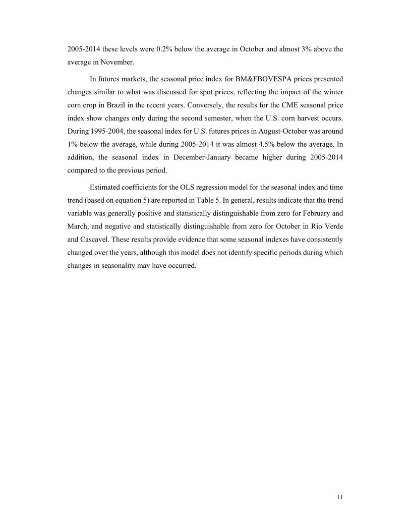
Estimated coefficients for the OLS regression model for the seasonal index and time

trend (based on equation 5) are reported in Table 5. In general, results indicate that the trend

variable was generally positive and statistically distinguishable from zero for February and

March, and negative and statistically distinguishable from zero for October in Rio Verde

and Cascavel. These results provide evidence that some seasonal indexes have consistently

changed over the years, although this model does not identify specific periods during which

changes in seasonality may have occurred.

12

Table 4: Seasonal corn price index during 1995-2004 and 2005-2014. Area Period Jan Feb Mar Apr May June July Aug Sept Oct Nov Dec Std Dev. Ampl.

Cascavel 1995-2004 99.87 97.87 96.34 99.87 101.35 97.78 95.91 98.63 100.71 103.74 106.66 101.80 3.10 10.742005-2014 101.99 104.40 101.91 99.53 99.44 99.71 97.69 96.06 98.23 97.43 101.90 102.03 2.45 8.34

Chapecó 1995-2004 100.85 95.71 95.08 97.59 99.55 96.77 95.22 98.03 102.80 105.41 108.99 105.13 4.58 13.922005-2014 102.83 102.26 99.97 97.01 97.08 97.17 96.39 97.04 101.32 101.38 104.78 103.26 2.98 8.39

Rio Verde 1995-2004 102.84 98.68 95.50 98.01 98.34 95.80 93.30 95.45 100.76 106.42 110.21 106.17 5.26 16.912005-2014 106.54 106.11 105.04 100.81 96.60 95.20 93.32 93.14 98.17 98.81 101.60 106.04 5.01 13.40

Mogiana 1995-2004 104.66 98.36 95.18 96.72 97.98 94.58 93.44 97.51 101.85 105.64 109.97 105.62 5.28 16.532005-2014 103.83 101.76 102.12 97.76 95.86 95.99 96.46 97.66 100.58 101.42 103.13 103.97 3.11 8.10

BM&F 1995-2004 96.11 91.94 93.78 98.14 98.86 95.82 96.16 99.23 106.56 111.04 110.74 103.81 6.40 19.102005-2014 101.12 99.37 98.37 96.63 98.09 97.17 96.31 98.25 102.54 101.35 105.11 106.28 3.27 9.97

CME 1995-2004 98.88 102.91 104.16 102.56 103.98 101.88 97.45 97.79 98.91 99.49 96.79 95.68 2.93 8.482005-2014 102.66 102.37 104.83 102.51 103.09 102.90 98.60 94.87 95.83 95.99 97.22 99.78 3.44 9.96

Spot Average

1995-2004 102.05 97.65 95.52 98.05 99.30 96.23 94.47 97.41 101.53 105.31 108.96 104.68 4.55 14.532005-2014 103.80 103.63 102.26 98.77 97.25 97.02 95.96 95.97 99.58 99.76 102.85 103.83 3.39 9.56

Table 5: Estimated regression model for corn price index considering each separated month (June 1995 – December 2014). Area Coeffic. Jan Feb Mar Apr May June July Aug Sept Oct Nov Dec

Cascavel c -0.017 -0.057 -0.069 -0.008 0.030 -0.005 -0.014 0.008 0.024 0.053 0.061 0.005

Trend 0.003 0.008 ** 0.007 ** 0.001 -0.003 -0.001 -0.001 -0.004 -0.003 -0.006 *** -0.003 0.001

Chapecó c 0.003 -0.063 *** -0.066 ** -0.029 0.015 -0.012 -0.021 -0.008 0.027 0.057 *** 0.076 0.044

Trend 0.002 0.006 *** 0.005 ** 0.001 -0.003 -0.002 -0.002 -0.002 -0.000 -0.003 -0.002 -0.001

Rio Verde

c 0.009 -0.042 -0.084 ** -0.048 -0.014 -0.028 -0.029 -0.017 0.020 0.079 ** 0.091 0.049

Trend 0.004 0.007 *** 0.010 * 0.005 -0.001 -0.002 -0.003 -0.004 -0.002 -0.007 ** -0.005 0.000

Mogiana c 0.049 -0.043 -0.097 ** -0.067 -0.018 -0.049 -0.042 -0.007 0.036 0.081 ** 0.098 ** 0.058

Trend -0.000 0.005 0.009 * 0.005 -0.001 0.000 -0.000 -0.002 -0.002 -0.006 -0.005 -0.002

BM&F c -0.054 -0.133 * -0.108 ** -0.027 0.004 -0.013 -0.025 -0.002 0.074 *** 0.122 ** 0.094 0.035

Trend 0.004 0.009 ** 0.007 0.000 -0.002 -0.002 -0.001 -0.001 -0.003 -0.008 -0.003 0.001

CME c -0.007 0.038 0.054 0.042 0.054 0.033 -0.011 -0.034 -0.032 -0.017 -0.047 -0.054

Trend 0.002 -0.001 -0.001 -0.001 -0.002 -0.001 -0.000 -0.000 0.001 -0.001 0.002 0.003

Note: ∗, ∗∗ and ∗∗∗ denote significance at the 1%, 5%, and 10% levels, respectively.

13

The seasonal index for BM&FBOVESPA basis is reported in Table 6 and Figure 2 (Appendix

A). Overall, the difference between highest and lowest indexes within the year was smaller in 2005-

2014 compared to 1995-2004 in all four regions. In particular, in all regions the seasonal indexes in

January-February were not as high in 2005-2014 as they used to be in 1995-2004. While January-

February in 1995-2004 presented an average seasonal index for BM&FBOVESPA basis around 8%

over the annual average, these values were around 3% over the annual average in 2005-2014. Further,

in 1995-2004 the seasonal indexes reached their lowest points in September-October in all regions.

But in 2005-2014 this behavior was observed only in Cascavel and Rio Verde. In the other two regions

(Chapecó and Mogiana), the seasonal indexes reached the lowest levels in May and then remained

within a narrow range until the end of the year.

Table 7 shows estimated coefficients for OLS regression model with the seasonal index and

time trend. Findings are mixed across regions and months, and no clear pattern emerges from

regression results. Overall, estimates were statistically distinguishable from zero for Cascavel in

February (negative) and June (positive), for Chapecó in February (negative) and September-October

(positive), for Rio Verde in April (positive) and November (negative), and for Mogiana in April

(positive) and November-December (negative).

14

Table 6: Seasonal index for BM&FBOVESPA basis during 1995-2004 and 2005-2014.

Area Period Jan Feb Mar Apr May June July Aug Sept Oct Nov Dec Std Dev. Ampl

Cascavel 1995-2004 106.60 110.04 104.42 101.18 101.01 100.74 98.02 97.55 92.88 92.58 96.73 99.71 5.16 17.46

2005-2014 100.92 105.08 103.65 102.98 101.38 102.59 101.43 97.76 95.80 96.15 96.90 95.97 3.34 9.29

Chapecó 1995-2004 106.21 106.46 102.93 99.63 99.11 99.86 97.67 97.71 95.86 94.42 98.60 102.33 3.77 12.04

2005-2014 101.71 102.91 101.66 100.35 98.96 100.00 100.13 98.74 98.82 100.06 99.66 97.13 1.56 5.78

Rio Verde 1995-2004 109.17 108.25 101.87 99.66 98.38 99.43 95.77 94.83 94.05 95.85 100.43 103.63 4.95 15.11

2005-2014 105.41 106.79 106.88 104.27 98.47 97.95 96.89 94.75 95.73 97.54 96.65 99.76 4.47 12.13

Mogiana 1995-2004 110.07 108.16 102.15 99.01 97.93 98.43 95.85 96.70 94.91 94.94 100.25 102.91 4.94 15.16

2005-2014 102.68 102.38 103.90 101.11 97.73 98.78 100.18 99.37 98.10 100.10 98.10 97.81 2.10 6.17

Average 1995-2004 108.01 108.23 102.84 99.87 99.11 99.61 96.83 96.70 94.42 94.45 99.00 102.14 4.70 14.942005-2014 102.68 104.29 104.02 102.18 99.13 99.83 99.66 97.65 97.11 98.46 97.83 97.67 2.87 8.34

Table 7: Estimated regression model for corn BM&FBOVESPA basis index considering each separated month (June 1995 – December 2014). Area Coeffic. Jan Feb Mar Apr May June July Aug Sept Oct Nov Dec

Cascavel c 0.065 *** 0.110 * 0.049 ** 0.005 0.003 -0.010 -0.012 -0.019 -0.075 * -0.078 * -0.027 -0.009

Trend -0.004 -0.005 *** -0.001 0.002 0.001 0.003 *** 0.002 -0.000 0.002 0.003 -0.001 -0.002

Chapecó c 0.064 *** 0.087 * 0.051 ** -0.005 -0.014 -0.017 -0.015 -0.024 -0.057 * -0.070 * -0.018 0.017

Trend -0.003 -0.005 *** -0.003 0.000 0.000 0.001 0.001 0.001 0.003 *** 0.005 ** 0.001 -0.003

Rio Verde c 0.085 *** 0.085 ** 0.011 -0.029 -0.035 ** -0.022 -0.019 -0.035 *** -0.060 ** -0.037 *** 0.006 0.028

Trend -0.002 -0.002 0.004 0.006 ** 0.002 0.001 -0.001 -0.002 0.001 0.001 -0.003 *** -0.002

Mogiana c 0.107 * 0.084 * 0.002 -0.041 ** -0.042 ** -0.039 ** -0.034 -0.030 -0.047 ** -0.037 0.017 0.035 ***

Trend -0.006 -0.004 0.003 0.005 ** 0.002 0.002 0.002 0.001 0.001 0.002 -0.003 *** -0.004 ***


15

Seasonal analysis for CME basis shows distinct results than for BM&FBOVESPA basis. In

2005-2014 seasonal indexes for CME basis were higher in the first quarter and lower in the last

quarter compared to what they used to be in 1995-2004. For example, in 1995-2004 the average

seasonal index for CME basis in March was almost 8% below the annual average, while in 2005-

2014 this index was almost at the annual average. In October, the seasonal index was around 12%

above the annual average during 1995-2004, but around 4% above the annual average during 2005-

2014. Further, the overall behavior within the year is similar in both periods, but the seasonal curve

seems to be shifted to the right during 2005-2014. Consequently, the lowest values for the seasonal

index were observed around June in 2005-2014, as opposed to April in 1995-2004.

Regression results for the OLS model with seasonal index and time trend have little to show.

Only for Rio Verde there are estimates that are statistically distinguishable from zero, for March

(positive) and October (negative).

16

Table 8: Seasonal index for CME basis during 1995-2004 and 2005-2014.

Area Period Jan Feb Mar Apr May June July Aug Sept Oct Nov Dec Std Dev. Ampl.

Cascavel 1995-2004 99.05 98.77 93.08 92.83 94.64 94.89 97.46 101.80 104.67 110.16 111.19 103.56 6.24 18.36

2005-2014 103.09 102.81 98.57 94.75 94.28 94.74 95.48 98.66 101.82 101.47 107.09 108.52 4.84 14.24

Chapecó 1995-2004 99.99 96.61 91.87 90.75 92.95 93.91 96.73 101.17 106.85 111.93 113.62 106.97 7.89 22.88

2005-2014 103.91 100.69 96.69 92.34 92.03 92.32 94.28 99.64 105.01 105.62 110.12 109.80 6.71 18.09

Rio Verde 1995-2004 101.95 99.57 92.30 91.16 91.80 92.98 94.80 98.51 104.70 113.00 114.90 108.05 8.33 23.74

2005-2014 107.69 104.51 101.59 95.95 91.58 90.46 91.22 95.63 101.74 102.95 106.81 112.74 7.24 22.27

Mogiana 1995-2004 103.79 99.25 92.03 89.92 91.47 91.78 94.97 100.63 105.81 112.18 114.65 107.45 8.51 24.73

2005-2014 104.95 100.19 98.78 93.04 90.88 91.22 94.35 100.30 104.23 105.65 108.39 110.51 6.72 19.63

Average 1995-2004 101.20 98.55 92.32 91.16 92.71 93.39 95.99 100.52 105.51 111.82 113.59 106.51 7.74 22.432005-2014 104.91 102.05 98.91 94.02 92.19 92.19 93.83 98.56 103.20 103.93 108.10 110.39 6.38 18.56

Table 9: Estimated regression model for corn CME basis index considering each separated month (June 1995 – December 2014).

Area Coeffic. Jan Feb Mar Apr May June July Aug Sept Oct Nov Dec

Cascavel c -0.029 -0.043 -0.093 *** -0.072 *** -0.043 -0.047 -0.005 0.047 0.072 0.114 ** 0.096 0.006

Trend 0.004 0.005 0.005 0.001 -0.002 -0.001 -0.002 -0.005 -0.004 -0.007 -0.002 0.004

Chapecó c -0.009 -0.049 -0.089 *** -0.093 ** -0.058 -0.055 -0.013 0.030 0.075 0.119 ** 0.110 *** 0.046

Trend 0.003 0.003 0.003 0.001 -0.002 -0.002 -0.003 -0.002 -0.002 -0.004 -0.001 0.003

Rio Verde c -0.003 -0.028 -0.107 ** -0.112 ** -0.088 ** -0.070 -0.021 0.021 0.067 0.141 * 0.125 *** 0.050

Trend 0.005 0.005 0.008 *** 0.005 0.000 -0.001 -0.005 -0.005 -0.004 -0.008 *** -0.004 0.004

Mogiana c 0.037 -0.029 -0.119 ** -0.131 * -0.092 ** -0.092 *** -0.033 0.031 0.083 0.143 ** 0.133 ** 0.060

Trend 0.001 0.003 0.008 0.004 0.000 0.000 -0.002 -0.002 -0.003 -0.007 -0.004 0.002


17

Market integration analysis

Unit root tests suggest that all price series were non-stationary in levels and stationary in

first-differences at the 1% significance level (Appendix B). Therefore, all series were

integrated of order one, I(1).

Results of the Engle-Granger bivariate cointegration procedure and Johansen

cointegration test generally indicate the presence of long-run relationship between Brazilian

spot and CME futures prices in the recent period (2005-2014), but not during 1995-2004

(Appendix B). Similar findings were observed for Brazilian and U.S. futures prices. On the

other hand, test results for Brazilian spot and futures prices showed evidence of

cointegration in both periods.

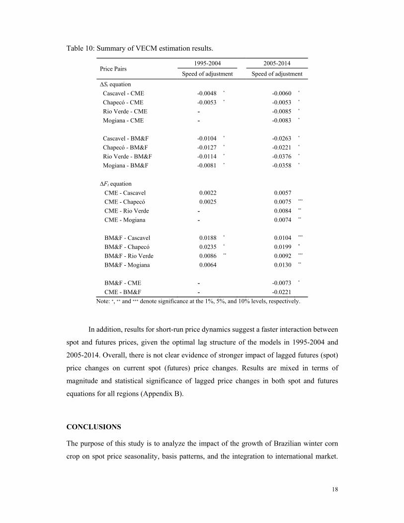
Next, VEC models were estimated for both periods, 1995-2004 and 2005-2014,

separately for each pair of spot and futures prices. Results for the spot-CME futures models

show that speed-of-adjustment coefficients were statistically significant and negative in the

∆St equations for all areas in both periods, but statistically significant and positive in three

∆Ft equations only in the second period (Table 10). These findings suggest that spot prices

always made the adjustment towards the long-run equilibrium, while CME futures prices

only started contributing to this adjustment process in the second period. The half-life

period3 of spot price responses to a random shock during 2004-2015 was 115, 130, 81, and

83 days for Cascavel, Chapecó, Rio Verde, and Mogiana, respectively, indicating a slow

adjustment process.

Table 10 also presents the results of speed-of-adjustment coefficients for spot-

BM&FBOVESPA futures price pairs. Speed-of-adjustment parameters were statistically

significant and negative in the ∆St equations and statistically significant and positive in the

∆Ft equations for both periods (except for Mogiana in the first period). Results show

evidence of a faster speed of adjustment for spot prices in 2005-2014 compared to 1995-

2004, with half-life decreasing around 60% from the first to the second period (from 67 days

to 24 days, on average).4

3 The half-life is the expected time for a shock to decay by 50%. It is a measure of speed of adjustment and is calculated using ln(0.5)/ln(1 – α).

4 Changes in the futures contracts, from physical delivery to cash settlement, may have also contributed to faster speed of adjustment.

18

Table 10: Summary of VECM estimation results.

Price Pairs 1995-2004 2005-2014

Speed of adjustment Speed of adjustment

∆St equation

Cascavel - CME -0.0048 * -0.0060 *

Chapecó - CME -0.0053 * -0.0053 *

Rio Verde - CME - -0.0085 *

Mogiana - CME - -0.0083 *

Cascavel - BM&F -0.0104 * -0.0263 *

Chapecó - BM&F -0.0127 * -0.0221 *

Rio Verde - BM&F -0.0114 * -0.0376 *

Mogiana - BM&F -0.0081 * -0.0358 *

∆Ft equation

CME - Cascavel 0.0022 0.0057

CME - Chapecó 0.0025 0.0075 ***

CME - Rio Verde - 0.0084 **

CME - Mogiana - 0.0074 **

BM&F - Cascavel 0.0188 * 0.0104 ***

BM&F - Chapecó 0.0235 * 0.0199 *

BM&F - Rio Verde 0.0086 ** 0.0092 ***

BM&F - Mogiana 0.0064 0.0130 **

BM&F - CME - -0.0073 *

CME - BM&F - -0.0221


In addition, results for short-run price dynamics suggest a faster interaction between

spot and futures prices, given the optimal lag structure of the models in 1995-2004 and

2005-2014. Overall, there is not clear evidence of stronger impact of lagged futures (spot)

price changes on current spot (futures) price changes. Results are mixed in terms of

magnitude and statistical significance of lagged price changes in both spot and futures

equations for all regions (Appendix B).

CONCLUSIONS

The purpose of this study is to analyze the impact of the growth of Brazilian winter corn

crop on spot price seasonality, basis patterns, and the integration to international market.

19

Four distinct spot markets in Brazil are investigated, along with two futures markets (Brazil

and US) to explore basis behavior.

Results from seasonality analysis for spot prices show that prices have been

oscillating within a narrower range in 2005-2014 compared to 1995-2004, in addition to

changes in seasonal patterns between the two periods. In the first quarter, spot prices are

now generally above the annual average, while they used to be below the annual average in

1995-2004. Further, spot prices still reach their lowest levels in July-August and then

increase in September-November in both periods. However, this price increase in

September-November in 2005-2014 is not as strong as it used to be in 1995-2004.

Seasonal analysis for BM&FBOVESPA basis also indicates a narrower range within

the year for 2005-2014 compared to the previous period. In all regions, the seasonal indexes

in January-February are not as high in 2005-2014 as they used to be in 1995-2004. In

addition, seasonal indexes reached their lowest points in September-October in all regions

in 1995-2004. However, in 2005-2014 this behavior was observed only in Cascavel and Rio

Verde. In the other two regions (Chapecó and Mogiana), the seasonal indexes reached the

lowest levels in May and then remained within a tight range until the end of the year. With

respect to the CME basis, results are distinct from findings for BM&FBOVESPA basis. The

overall behavior of the CME basis within the year is mostly similar in both periods, with

two distinctions. Seasonal indexes in the first and last quarter are respectively higher and

lower in 2005-2014 compared to 1995-2004. Further, seasonal curves seem to be shifted to

the right during 2005-2014, i.e. the lowest values for the seasonal indexes are now observed

around June, as opposed to April in 1995-2004.

The findings described above appear to be stronger in southern and south-eastern

Brazil. In the center-west area (Rio Verde), there is a relatively smaller change in basis range

within the year. This suggests greater unpredictability for Rio Verde-BM&FBOVESPA

basis (i.e. higher basis risk) compared to other areas, which may impact hedging

effectiveness in BM&FBOVESPA futures market.

With respect to market integration, overall results suggest that Brazilian corn prices are

experiencing higher integration to international prices in the more recent period. In general,

cointegration tests indicate that Brazilian corn prices and CME futures prices have shared

common long-run information since mid-2000’s, which coincides with a large increase of

Brazilian production and exports stimulated by the expansion of winter corn crop. Thus,

both spot and CME futures prices now adjust to reestablish their long-run equilibrium

20

relationship, whereas only spot prices used to make the adjustment in 1995-2004. Regarding

spot and BM&FBOVESPA futures prices, both prices participate in the adjustment to their

long-run equilibrium in both periods. Finally, comparison of speed-of-adjustment

coefficients for spot-CME futures and spot-BM&FBOVESPA futures prices pair reveals

faster adjustment in the relationship spot-BM&FBOVESPA futures price. The half-life

period of shocks associated to spot-BM&FBOVESPA futures prices (24 days, on average)

was lower than the result obtained in the spot-CME futures prices pair (102 days, on

average).

These changes in seasonal patterns and spot-futures prices relationships have

implications to marketing and risk management strategies. In principle, stronger relationship

between spot and futures markets suggest more effective opportunities for futures hedging.

The next steps of this research are to explore current effectiveness of marketing strategies

used in the past compared to what it used to be in 1995-2004, and to investigate new

strategies taking into account new price and basis patterns.

REFERENCES

Baffes, J. and B. Gardner (2003). The transmission of world commodity prices to domestic

markets under policy reforms in developing countries. The Journal of Policy Reform,

6, 159-180.

Balcombe, K., A. Bailey, and J. Brooks (2007). Threshold effects in price transmission: the

case of Brazilian wheat, maize, and soya prices. American Journal of Agricultural

Economics, 89, 308-323.

Bekkerman, A. and D. Pelletier (2009). Basis volatilities in corn and soybeans in spatially

separated markets: the effect of ethanol demand. Proceedings of the AAEA & ACCI

Annual Meeting, Milwaukee, WI.

Booth, G. G. and C. Ciner (1997). International transmission on information in corn futures

markets. Journal of Multinational Financial Management, 7, 175-187.

Booth, G. G., P. Brockman, and Y. Tse (1998). The relationship between US and Canadian

wheat futures. Applied Financial Economics, 8, 73-80.

Cheung, Y-W and L.K. Ng (1996). A causality in variance test and its application to

financial market prices. Journal of Econometrics, 72, 33-48.

21

Crain, S. J. and J. H. Lee (1996). Volatility in wheat spot and futures markets, 1950–1993:

government farm programs, seasonality, and causality. The Journal of Finance, 51, 325-

343.

Esposti, R. and Listorti, G. (2013). Agricultural price transmission across space and

commodities during price bubbles. Agricultural Economics, 44, 125-139.

Fossati, S., F. Lorenzo, and C. M. Rodriguez (2007). Regional and international market

integration of a small open economy. Journal of Applied Economics, 10, 77-98.

Goetz, S. and M. Weber (1986). Fundamentals of price analysis in developing countries.

Food systems: A training manual to accompany the microcomputer software program

MSTAT. MSU International Development Papers. Working Paper 29, Department of

Agricultural Economics, Michigan State University.

Goychuk, K. and W. H. Meyers (2011). Black sea wheat market integration with the

international wheat markets: some evidence from co-integration analysis. Proceedings

of Agricultural and Applied Economics Association Annual Meeting, July 24-26, 2011,

Pittsburgh, Pennsylvania.

Jiang, B., and M. Hayenga (1997). Corn and soybean basis behavior and forecasting:

fundamental and alternative approaches. Proceedings of the NCR-134 Conference on

Applied Commodity Price Analysis, Forecasting, and Market Risk Management,

Chicago, IL.

Liu, Q. and Y, An (2011). Information transmission in informationally linked markets:

Evidence from US and Chinese commodity futures markets. Journal of International

Money and Finance, 30, 778-795

Mundlak, Y. and D. F. Larson (1992). On the transmission of world agricultural prices.

World Bank Economic Review, 6, 399-422.

Nazlioglu. S., C. Erdem, and U. Soytas (2013). Volatility spillover between oil and

agricultural commodity markets. Energy Economics, 36, 658-665.

Rapsomanikis, G., D. Hallam, and P. Conforti (2006). Market integration transmission in

selected food and cash crop markets of developing countries: review and applications.

In: Sarris, A. and Hallam, D. Agricultural Commodity Markets and Trade: New

Approaches to Analyzing Market Structure and Instability.

22

Sanders, D. R., and T. D. Greer (2003). Hedging spot corn: an examination of the

Minneapolis grain exchange’s cash settled corn contract. Journal of Agribusiness, 21,

65-81.

Sarfo, S. and H. Geman (2012). Seasonality in cocoa spot and forward markets: empirical

evidence. Journal of Agricultural Extension and Rural Development, 4, 164-180.

Schroeder, T.C. (1997). Fed cattle spatial transactions price relationships. Journal of

Agricultural and Applied Economics, 29, 347–62.

Seamon, V. F., K. H. Kahl, and C. E. Curtis Jr (2001). Regional and seasonal differences in

the cotton basis. Journal of Agribusiness, 19, 147-161.

Sorensen, C. (2002). Modelling seasonality in agricultural commodity futures. Journal of

Futures Markets, 22, 393-426.

Yang. J., J. Zhang, and D. J. Leatham (2003). Price and volatility transmission in

international wheat futures markets. Annals of Economics and Finance, 4, 37-50.

Zakari, S., L. Ying, and B. Song. (2014). Market integration and spatial price transmission

in Niger grain markets. African Development Review, 26, 264-273.

23

Appendix A. Figures

Figure A1: Seasonal price index during 1995-2004 and 2005-2014.

(a) Cascavel (b) Chapecó

(a) Rio Verde (b) Mogiana

(a) BM&FBOVESPA (b) CME

24

Figure A2: Seasonal BM&FBOVESPA basis index during 1995-2004 and 2005-2014.


(c) Rio Verde (d) Mogiana

Figure A3: Seasonal CME basis index during 1995-2004 and 2005-2014.


(c) Rio Verde (d) Mogiana

25

Appendix B. Tables

Table B1: Unit root tests for daily corn log-prices during 1995-2004 and 2005-2014.

Level Prices 1st Difference of Prices

With Trend Without Trend With Trend Without Trend

ADF(a) PP(b) ADF(a) PP(b) ADF(a) PP(b) ADF(a) PP(b)

1995-2004 period

Cascavel -2.09 -2.20 -2.09 -1.66 -13.39 * -61.35 * -13.38 * -61.39 *

Chapecó -2.29 -2.20 -2.29 -1.51 -12.49 * -62.31 * -12.49 * -62.44 *

R.Verde -2.36 -2.06 -2.36 -1.71 -10.69 * -61.11 * -10.66 * -61.14 *

Mogiana -2.46 -2.15 -2.46 -1.81 -13.09 * -62.18 * -13.07 * -62.22 *

BM&F -2.18 -2.45 -2.18 -1.50 -44.32 * -44.47 * -44.33 * -44.48 *

CME -2.02 -2.08 -2.02 -1.67 -44.00 * -44.06 * -44.00 * -44.07 *

2005-2014 period

Cascavel -2.84 -2.82 -2.84 -2.37 -19.82 * -41.53 * -19.82 * -41.53 *

Chapecó -2.92 -2.57 -2.92 -2.04 -14.37 * -51.32 * -14.37 * -51.34 *

R. Verde -2.36 -2.81 -2.36 -2.44 -21.99 * -52.41 * -21.99 * -52.41 *

Mogiana -2.00 -2.55 -2.00 -2.22 -54.33 * -54.60 * -54.33 * -54.61 *

BM&F -2.90 -3.26 -2.90 -2.47 -44.35 * -45.02 * -44.36 * -45.03 *

CME -2.38 -2.38 -2.38 -1.76 -48.70 * -48.71 * -48.71 * -48.72 *

a Unit root test developed by Dickey and Fuller (1981). The optimal lags selected in the test were based on the Schwartz criterion. b Unit root test developed by Phillips and Perron (1988). Note: ∗, ∗∗ and ∗∗∗ denote significance at the 1%, 5%, and 10% levels, respectively.

Table B2: Engle-Granger tests for cointegration between corn price pairs.

Price Pair 1995-2004 2005-2014

CRADF CRADF

Cascavel – CME -2.76 -3.49 **

Chapecó – CME -2.57 -3.49 **

R.Verde – CME -2.51 -4.16 *

Mogiana – CME -2.50 -3.72 **

BM&F – CME -2.80 -3.79 **

Cascavel – BM&F -5.03 * -6.86 *

Chapecó – BM&F -5.61 * -6.61 *

R.Verde – BM&F -4.37 * -7.22 *

Mogiana – BM&F -4.15 * -7.59 *

CME – BM&F -2.75 -3.67 **


26

Table B3: Johansen tests for cointegration between corn price pairs.

Price Pairs Null

Hypothesis

1995-2004 2005-2014

Max-Eigen Stat.

Trace Stat. Max-Eigen

Stat. Trace Stat.

Cascavel - CME r = 1 15.32 ** 18.11 ** 16.65 ** 19.56 **

r ≤ 1 2.79 *** 2.79 *** 2.90 *** 2.90 ***

Chapecó - CME r = 1 13.02 *** 15.39 *** 14.33 ** 17.52 **

r ≤ 1 2.38 2.38 3.18 *** 3.18 ***

R.Verde - CME r = 1 12.16 14.73 *** 15.48 ** 19.20 **

r ≤ 1 2.57 2.57 3.72 *** 3.72 ***

Mogiana - CME r = 1 10.19 13.00 16.10 ** 19.82 *

r ≤ 1 2.81 2.81 3.71 *** 3.71 **

BM&F - CME r = 1 10.91 12.80 16.81 ** 19.70 **

r ≤ 1 1.89 1.89 2.89 *** 2.89 ***

Cascavel - BM&F r = 1 27.21 * 30.04 * 79.17 * 15.49 *

r ≤ 1 2.83 *** 2.83 *** 6.19 ** 6.19 **

Chapecó - BM&F r = 1 33.22 * 35.53 * 85.46 * 91.03 *

r ≤ 1 2.32 2.32 5.57 ** 5.57 **

R.Verde - BM&F r = 1 17.89 ** 21.55 * 66.82 * 73.17 *

r ≤ 1 3.66 *** 3.66 *** 6.35 ** 6.35 **

Mogiana - BM&F r = 1 21.59 * 24.31 * 52.78 * 58.61 *

r ≤ 1 2.81 *** 2.81 *** 5.88 ** 5.88 **

CME - BM&F r = 1 10.91 12.81 16.81 ** 19.70 **

r ≤ 1 1.89 1.89 2.89 *** 2.89 ***


27

Table B4: Error-correction model parameter estimates for Cascavel.

Cascavel-CME CME-Cascavel Cascavel-BM&F BM&F-Cascavel

∆St 1995-2004

∆St 2005-2014

∆Ft

1995-2004 ∆Ft

2005-2014

∆St 1995-2004

∆St 2005-2014

∆Ft

1995-2004 ∆Ft

2005-2014

C 0.0002 0,0001 0.0002 0.0003 0.0001 0.0001 0.0003 0.0001

Coint. Eq. -0.0048 * -0.0060 * 0.0022 0.0057 -0.0104 * -0.0262 * 0.0188 * 0.0104 ***

∆St-1 -0.1593 * 0.2045 * 0.0416 -0.0179 *** -0.1286 * 0.1829 * 0.1094 ** 0.0736 **

∆St-2 0.1124 * 0.1390 * -0.0083 -0.0770 ** 0.1166 * 0.1159 * 0.0494 0.0389

∆St-3 0.1797 * 0.0937 * 0.0362 0.1135 0.1312 * 0.0671 * 0.0333 0.0679 ***

∆St-4 0.0913 * 0.0561 * -0.0967 ** -0.0076 0.0613 * 0.0365 ** 0.0976 **

∆St-5 0.0748 * 0.0067 0.0629 * 0.0996 **

∆St-6 0.0574 * -0.0302 0.0794 * 0.0461

∆St-7 0.0607 * 0.0396 0.0502 ** 0.0328

∆St-8 0.0428 ** 0.0328 0.0254 0.0155

∆St-9 0.0214 0.1017 **

∆St-10 0.0106 0.0148

∆Ft-1 0.0171 0.0545 * 0.0998 * 0.0140 0.0194 *** 0.0676 * -0.0005 0.0326

∆Ft-2 0.0130 0.0437 * -0.0184 -0.0170 0.0143 0.0326 * 0.0469 ** 0.0984 *

∆Ft-3 0.0344 * 0.0150 0.0076 0.0068 0.0198 *** 0.0188 0.0060 0.0124

∆Ft-4 0.0087 0.0061 0.0121 0.0107 0.0344 * 0.0148 -0.0255 0.0248

∆Ft-5 0.0083 0.0132 0.0101 0.0333 0.0063

∆Ft-6 0.0016 0.0014 0.0117 0.0482 **

∆Ft-7 0.0061 -0.0116 0.0091 -0.0334

∆Ft-8 -0.0019 0.0394 *** 0.0111 0.0007

∆Ft-9 -0.0067 0.0421 **

∆Ft-10 -0.0041 -0.0448 **

Wald F stat. 1.2967 6.3253 * 1.7263 *** 2.5856 *** 0.5504 4.1355 * 0.5674 0.2989


28

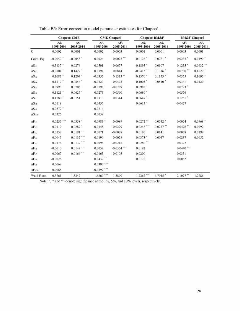
Table B5: Error-correction model parameter estimates for Chapecó.

Chapecó-CME CME-Chapecó Chapecó-BM&F BM&F-Chapecó

∆St 1995-2004

∆St 2005-2014

∆Ft

1995-2004 ∆Ft

2005-2014

∆St 1995-2004

∆St 2005-2014

∆Ft

1995-2004 ∆Ft

2005-2014

C 0.0002 0.0001 0.0002 0.0003 0.0001 0.0001 0.0003 0.0001

Coint. Eq. -0.0052 * -0.0053 * 0.0024 0.0075 *** -0.0126 * -0.0221 * 0.0235 * 0.0199 *

∆St-1 -0.3137 * 0.0274 0.0501 0.0677 -0.1895 * 0.0107 0.1235 * 0.0932 **

∆St-2 -0.0804 * 0.1429 * 0.0194 0.0814 -0.0413 *** 0.1316 * 0.0730 *** 0.1629 *

∆St-3 0.1083 * 0.1204 * -0.0355 0.1313 ** 0.1370 * 0.1153 * 0.0355 0.1095 *

∆St-4 0.1217 * 0.0856 * -0.0320 0.0475 0.1005 * 0.0810 * 0.0361 0.0420

∆St-5 0.0993 * 0.0703 * -0.0798 * -0.0789 0.0982 * 0.0793 **

∆St-6 0.1121 * 0.0627 * 0.0273 -0.0560 0.0680 * 0.0576

∆St-7 0.1580 * -0.0151 0.0313 0.0344 0.0647 * 0.1261 *

∆St-8 0.0118 0.0457 0.0613 * -0.0427

∆St-9 0.0572 * -0.0214

∆St-10 0.0326 0.0039

∆Ft-1 0.0255 *** 0.0358 * 0.0983 * 0.0089 0.0272 ** 0.0542 * 0.0024 0.0968 *

∆Ft-2 0.0119 0.0287 * -0.0148 -0.0229 0.0248 *** 0.0237 ** 0.0476 ** 0.0092

∆Ft-3 0.0158 0.0191 ** 0.0071 -0.0028 0.0186 0.0141 0.0078 0.0199

∆Ft-4 0.0045 0.0132 *** 0.0190 0.0028 0.0373 * 0.0047 -0.0237 0.0052

∆Ft-5 0.0176 0.0139 *** 0.0098 -0.0245 0.0280 ** 0.0322

∆Ft-6 -0.0010 0.0147 *** 0.0058 -0.0354 *** 0.0192 0.0440 ***

∆Ft-7 0.0067 0.0164 ** -0.0163 0.0105 -0.0200 -0.0331

∆Ft-8 -0.0026 0.0432 ** 0.0178 0.0062

∆Ft-9 0.0069 0.0390 ***

∆Ft-10 0.0088 -0.0397 ***

Wald F stat. 0.3761 1.3247 1.6860 *** 1.5899 1.7262 *** 4.7045 * 2.1077 ** 1.2786


29

Table B6: Error-correction model parameter estimates for Rio Verde.

RV-CME CME-RV RV-BM&F BM&F-RV

∆St 2005-2014 ∆Ft

2005-2014 ∆St

1995-2004 ∆St

2005-2014 ∆Ft

1995-2004 ∆Ft

2005-2014

C 0.0001 0.0003 0.0001 0.0002 0.0003 0.0001

Coint. Eq. -0.0085 * 0.0084 ** -0.0113 * -0.0376 * 0.0086 ** 0.0092 ***

∆St-1 -0.0644 * -0.0022 -0.1669 * -0.0764 * 0.0561 *** 0.0013

∆St-2 0.0176 0.0216 -0.0592 * 0.0049 0.0531 *** 0.0228

∆St-3 0.0425 ** 0.0490 *** 0.0209 0.0276 0.0577 *** 0.0187

∆St-4 0.0474 ** -0.0069 0.0417 *** 0.0303 0.0403 -0.0006

∆St-5 -0.0897 * -0.0072 0.0741 * -0.1059 * 0.0734 ** 0.0189

∆St-6 0.0185 0.0068 0.0926 * -0.0017 0.1386 * -0.0024

∆St-7 0.0698 * 0.0270 0.0978 * 0.0512 * 0.0550 *** 0.0138

∆St-8 0.0446 ** 0.0047 0.0496 ** 0.0289 0.0555 *** -0.0046

∆St-9 0.0594 * 0.0546 ** 0.0629 * 0.0442 ** -0.0429 -0.0055

∆St-10 0.0170 0.0136 0.0268 0.0055 -0.0805 * 0.0115

∆St-11 0.0419 *** 0.0028

∆St-12 0.0570 ** 0.0128

∆St-13 0.0071 -0.0008

∆Ft-1 0.0082 0.0105 0.0099 0.0336 -0.0090 0.1081 *

∆Ft-2 0.0356 ** -0.0216 0.0433 ** 0.0118 0.0441 *** 0.0234

∆Ft-3 0.0499 * -0.0001 0.0232 -0.0018 0.0047 0.0384 ***

∆Ft-4 0.0390 ** 0.0107 0.0223 0.0131 -0.0263 0.0203

∆Ft-5 0.0310 ** -0.0174 0.0219 0.0399 *** 0.0286 0.0332

∆Ft-6 0.0315 ** -0.0347 *** -0.0075 0.0440 ** 0.0429 *** 0.0099

∆Ft-7 0.0216 0.0106 0.0115 0.0269 -0.0350 -0.0180

∆Ft-8 0.0375 ** -0.0066 0.0250 0.0200 -0.0013 0.0317

∆Ft-9 -0.0097 0.0010 0.0266 -0.0251 -0.0089 -0.0244

∆Ft-10 0.0206 0.0168 -0.0019 0.0436 ** 0.0012 0.0651 *

∆Ft-11 0.0400 ** 0.0006

∆Ft-12 0.0363 ** -0.0013

∆Ft-13 -0.0089 -0.0128

Wald F stat. 1.2411 0.7418 0.9923 1.1686 2.4686 * 3.3158 *


30

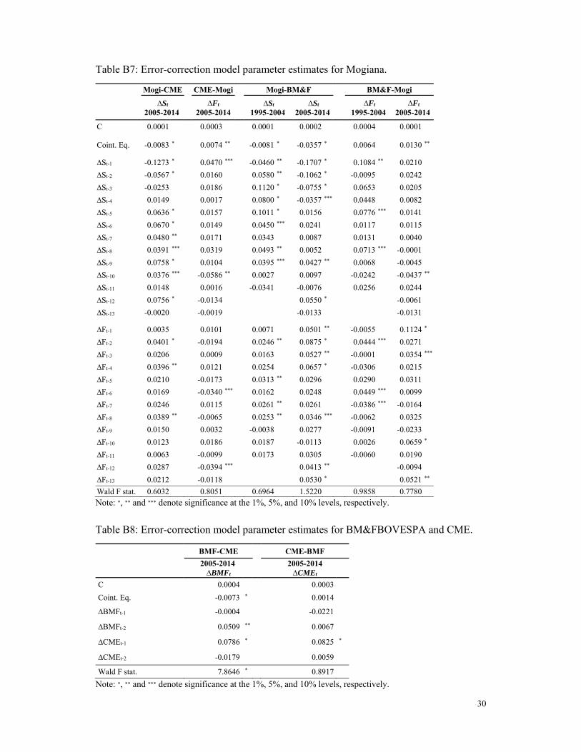
Table B7: Error-correction model parameter estimates for Mogiana.

Mogi-CME CME-Mogi Mogi-BM&F BM&F-Mogi

∆St 2005-2014

∆Ft

2005-2014

∆St 1995-2004

∆St 2005-2014

∆Ft

1995-2004 ∆Ft

2005-2014

C 0.0001 0.0003 0.0001 0.0002 0.0004 0.0001

Coint. Eq. -0.0083 * 0.0074 ** -0.0081 * -0.0357 * 0.0064 0.0130 **

∆St-1 -0.1273 * 0.0470 *** -0.0460 ** -0.1707 * 0.1084 ** 0.0210

∆St-2 -0.0567 * 0.0160 0.0580 ** -0.1062 * -0.0095 0.0242

∆St-3 -0.0253 0.0186 0.1120 * -0.0755 * 0.0653 0.0205

∆St-4 0.0149 0.0017 0.0800 * -0.0357 *** 0.0448 0.0082

∆St-5 0.0636 * 0.0157 0.1011 * 0.0156 0.0776 *** 0.0141

∆St-6 0.0670 * 0.0149 0.0450 *** 0.0241 0.0117 0.0115

∆St-7 0.0480 ** 0.0171 0.0343 0.0087 0.0131 0.0040

∆St-8 0.0391 *** 0.0319 0.0493 ** 0.0052 0.0713 *** -0.0001

∆St-9 0.0758 * 0.0104 0.0395 *** 0.0427 ** 0.0068 -0.0045

∆St-10 0.0376 *** -0.0586 ** 0.0027 0.0097 -0.0242 -0.0437 **

∆St-11 0.0148 0.0016 -0.0341 -0.0076 0.0256 0.0244

∆St-12 0.0756 * -0.0134 0.0550 * -0.0061

∆St-13 -0.0020 -0.0019 -0.0133 -0.0131

∆Ft-1 0.0035 0.0101 0.0071 0.0501 ** -0.0055 0.1124 *

∆Ft-2 0.0401 * -0.0194 0.0246 ** 0.0875 * 0.0444 *** 0.0271

∆Ft-3 0.0206 0.0009 0.0163 0.0527 ** -0.0001 0.0354 ***

∆Ft-4 0.0396 ** 0.0121 0.0254 0.0657 * -0.0306 0.0215

∆Ft-5 0.0210 -0.0173 0.0313 ** 0.0296 0.0290 0.0311

∆Ft-6 0.0169 -0.0340 *** 0.0162 0.0248 0.0449 *** 0.0099

∆Ft-7 0.0246 0.0115 0.0261 ** 0.0261 -0.0386 *** -0.0164

∆Ft-8 0.0389 ** -0.0065 0.0253 ** 0.0346 *** -0.0062 0.0325

∆Ft-9 0.0150 0.0032 -0.0038 0.0277 -0.0091 -0.0233

∆Ft-10 0.0123 0.0186 0.0187 -0.0113 0.0026 0.0659 *

∆Ft-11 0.0063 -0.0099 0.0173 0.0305 -0.0060 0.0190

∆Ft-12 0.0287 -0.0394 *** 0.0413 ** -0.0094

∆Ft-13 0.0212 -0.0118 0.0530 * 0.0521 **

Wald F stat. 0.6032 0.8051 0.6964 1.5220 0.9858 0.7780


Table B8: Error-correction model parameter estimates for BM&FBOVESPA and CME.

BMF-CME CME-BMF

2005-2014 ∆BMFt

2005-2014 ∆CMEt

C 0.0004 0.0003

Coint. Eq. -0.0073 * 0.0014

∆BMFt-1 -0.0004 -0.0221

∆BMFt-2 0.0509 ** 0.0067

∆CMEt-1 0.0786 * 0.0825 *

∆CMEt-2 -0.0179 0.0059

Wald F stat. 7.8646 * 0.8917


The Effects of Brazilian Second (Winter) Corn Crop on ... · The Effects of Brazilian Second...

Documents

Transcript of The Effects of Brazilian Second (Winter) Corn Crop on ... · The Effects of Brazilian Second...