The Effective Theory of Inflationand Dark Matter in the Standard

Model of the UniverseH. J. de Vega

LPTHE, CNRS/Universit e Paris VI

Pennsylvannia State University, University Park, March 31 , 2010

– p. 1

The History of the UniverseIt is a history of EXPANSION and cooling down.

EXPANSION: the space itself expands with the time.

ds2 = dt2 − a 2(t) d~x2 , a(t) = scale factor.

FRW: Homogeneous, isotropic and spatially flat geometry.

Cooling: temperature decreases as 1/a(t): T (t) ∼ 1/a(t).

The Universe underwent a succesion of phase transitionstowards the less symmetric phases.

Wavelenghts redshift as a(t) : λ(t) = a(t) λ(t0)a(t0)

Redshift z : z + 1 = a(today)a(t) , a(today) ≡ 1

The deeper you go in the past, the larger is the redshift andthe smaller is a(t).

– p. 2

Standard Cosmological Model:ΛCDM

ΛCDM = Cold Dark Matter + Cosmological Constant

Begins by the inflationary era. Slow-Roll inflationexplains horizon and flatness.

Gravity is described by Einstein’s General Relativity.

Particle Physics described by the Standard Model ofParticle Physics: SU(3) ⊗ SU(2) ⊗ U(1) =qcd+electroweak model.

CDM: dark matter is cold (non-relativistic) during thematter dominated era where structure formationhappens. DM is outside the SM of particle physics.

Dark energy described by the cosmological constant Λ.

– p. 3

Standard Cosmological Model:ΛCDM

ΛCDM = Cold Dark Matter + Cosmological Constantbegins by the Inflationary Era. Explains the Observations:

Seven years WMAP data and further CMB data

Light Elements Abundances

Large Scale Structures (LSS) Observations. BAO.

Acceleration of the Universe expansion:Supernova Luminosity/Distance and Radio Galaxies.

Gravitational Lensing Observations

Lyman α Forest Observations

Hubble Constant (H0) Measurements

Properties of Clusters of Galaxies

Measurements of the Age of the Universe

– p. 4

Standard Cosmological Model: Concordance Model

ds2 = dt2 − a2(t) d~x 2: spatially flat geometry.

The Universe starts by an INFLATIONARY ERA .Inflation = Accelerated Expansion: d2a

dt2 > 0.During inflation the universe expands by at least sixtyefolds: e62 ≃ 1027. Inflation lasts ≃ 10−36 sec and ends byz ∼ 1029 followed by a radiation dominated era.Energy scale when inflation starts ∼ 1016 GeV ( ⇐= CMBanisotropies) which coincides with the GUT scale.Matter can be effectively described during inflation by aScalar Field φ(t,x): the Inflaton.

Lagrangean: L = a3(t)[

φ2

2 − (∇φ)2

2 a2(t) − V (φ)]

.

Friedmann eq.: H2(t) = 13 M2

Pl

[

φ2

2 + V (φ)]

, H(t) ≡ a(t)/a(t)

– p. 5

Inflation Evolution Equations

Evolution equation for the Inflaton:φ+ 3H(t) φ− 1

a2(t) ∇2φ+ V ′(φ) = 0 , H(t) ≡ a(t)a(t) = Hubble.

energy density = ρ = 12

[

φ2 + 1a2(t) (∇φ)2

]

+ V (φ)

pressure = p = 12

[

φ2 − 13 a2(t) (∇φ)2

]

− V (φ)

The scale factor grows exponentially during inflation andsuppresses spatial gradient terms.

The inflaton field is therefore homogeneous: φ = φ(t).φ+ 3H(t) φ+ V ′(φ) = 0 (1)

The Einstein equations reduce to a single equation: theFriedmann equation:

H2(t) = 13 M2

Pl

ρ = 13 M2

Pl

[

φ2

2 + V (φ)]

(2)

– p. 6

Physics during InflationOut of equilibrium evolution in a fastly expandinggeometry. Vacuum energy DOMINATED (De Sitter)universe a(t) ≃ eH t.

Explosive particle production due to spinodal orparametric instabilities. Quantum non-linearphenomena eventually shut-off the instabilities and stopinflation. Radiation dominated era follows: a(t) =

√t .

Huge redshift classicalizes the dynamics: an assemblyof (superhorizon) quantum modes behave as a classicaland homogeneous inflaton field. Inflaton slow-roll.

D. Boyanovsky, C. Destri, H. J. de Vega, N. G. Sánchez,The Effective Theory of Inflation in the Standard Model ofthe Universe and the CMB+LSS data analysis (reviewarticle), arXiv:0901.0549, Int.J.Mod.Phys.A 24, 3669-3864(2009).

– p. 7

The Theory of Inflation

The inflaton is an effective field in the Ginsburg-Landausense.

Relevant effective theories in physics:

Ginsburg-Landau theory of superconductivity. It is aneffective theory for Cooper pairs in the microscopicBCS theory of superconductivity.

The O(4) sigma model for pions, the sigma and photonsat energies . 1 GeV. The microscopic theory is QCD:quarks and gluons. π ≃ qq , σ ≃ qq .

The theory of second order phase transitions à laLandau-Kadanoff-Wilson... (ferromagnetic,antiferromagnetic, liquid-gas, Helium 3 and 4, ...)

Fermi Theory of Weak Interactions (current-current).

– p. 8

Slow Roll Inflation

The field evolves towards the minimum of the potential.

V (Min) = V ′(Min) = 0 : inflation ends after a finite numberof efolds. Slow-roll is needed to produce enough efolds ofinflation (≥ 62) to explain the part of todays’s entropy in theuniverse having a primordial origin.=⇒ the slope of the potential V (φ) must be small.

– p. 9

Slow-roll evolution of the InflatonDuring slow-roll the inflaton derivatives are small and theevolution equations (1) and (2) can be approximated by:

3H(t) φ+ V ′(φ) = 0 , H2(t) = V (φ)3M2

Pl

These first order equations can be solved in closed from as:

M2Pl N [φ] = −

∫ φend

φ V (ϕ)dϕdV

dϕ .

N [φ] = the number of e-folds since the field φ exits thehorizon till the end of inflation. N ∼ 60.φend = absolute minimum of V (φ).

Therefore, φ2 = scales as N M2Pl. We define:

χ ≡ φ√N MPl

dimensionless and slow field.

Universal form of the slow-roll inflaton potential:V (φ) = N M4 w(χ) , M = energy scale of inflation.

– p. 10

Primordial Power Spectrum

Adiabatic Scalar Perturbations: P (k) = |∆(S)k ad|2 kns−1 .

To dominant order in slow-roll:

|∆(S)k ad|2 = N2

12 π2

(

MMPl

)4w3(χ)w′2(χ) .

Hence, for all slow-roll inflation models:

|∆(S)k ad| ∼ N

2 π√

3

(

MMPl

)2

The WMAP7 result: |∆(S)k ad| = (0.494 ± 0.01) × 10−4

determines the scale of inflation M (using N ≃ 60)(

MMPl

)2= 0.85 × 10−5 −→ M = 0.70 × 1016 GeV

The inflation energy scale turns to be the grand unificationenergy scale !! We find the scale of inflation withoutknowing the tensor/scalar ratio r !!The scale M is independent of the shape of w(χ).

– p. 11

spectral indexns and the ratio r

r ≡ ratio of tensor to scalar fluctuations.tensor fluctuations = primordial gravitons.

ns − 1 = − 3

N

[

w′(χ)

w(χ)

]2

+2

N

w′′(χ)

w(χ), r =

8

N

[

w′(χ)

w(χ)

]2

dns

d ln k= − 2

N2

w′(χ) w′′′(χ)

w2(χ)− 6

N2

[w′(χ)]4

w4(χ)+

8

N2

[w′(χ)]2 w′′(χ)

w3(χ),

χ is the inflaton field at horizon exit.ns−1 and r are always of order 1/N ∼ 0.02 (model indep.)Running of ns of order 1/N2 ∼ 0.0003 (model independent).

D. Boyanovsky, H. J. de Vega, N. G. Sanchez,Phys. Rev. D 73, 023008 (2006), astro-ph/0507595.

– p. 12

Ginsburg-Landau ApproachGinsburg-Landau potentials:polynomials in the field starting by a constant term.

Linear terms can always be eliminated by a constant shift ofthe inflaton field.

The quadratic term can have a positive or a negative sign:

w′′(0) > 0 → single well potential → large field (chaotic) inflation

w′′(0) < 0 → double well potential → small field (new) inflation

The inflaton potential must be bounded from below =⇒highest order term must be even with a positive coefficient.

Renormalizability =⇒ degree of the inflaton potential ≤ 4.

The theory of inflation is an effective theory =⇒higher degree potentials are acceptable

– p. 13

Fourth order Ginsburg-Landau inflationary models

w(χ) = wo ± χ2

2 +G3 χ3 +G4 χ

4 , G3 = O(1) = G4

V (φ) = N M4 w(

φ√N MPl

)

= Vo ± m2

2 φ2 + g φ3 + λ φ4 .

m = M2

MPl, g = m√

N

(

MMPl

)2G3 , λ = G4

N

(

MMPl

)4

Notice that(

MMPl

)2≃ 10−5 ,

(

MMPl

)4≃ 10−10 , N ≃ 60 .

Small couplings arise naturally as ratio of two energyscales: inflation and Planck.

The inflaton is a light particle:m = M2

MPl≃ 0.003 M , m = 2.5 × 1013 GeV

H ∼√N m ≃ 2 × 1014 GeV.

– p. 14

WMAP 5 years data set plus other CMB data

Theory and observations nicely agree except for the lowestmultipoles: the quadrupole suppression.

– p. 15

MCMC Results for the double–well inflaton potential

ns

r

0.9 0.92 0.94 0.96 0.98 1 1.02 1.040

0.05

0.1

0.15

0.2

0.25

0.3

Solid line for N = 50 and dashed line for N = 60White dots: z = 0.01 + 0.11 ∗ n, n = 0, 1, . . . , 9,y increases from the uppermost dot y = 0, z = 1.

– p. 16

MCMC Results for double–well inflaton potential

Bounds: r > 0.023 (95% CL) , r > 0.046 (68% CL)Most probable values: ns ≃ 0.964, r ≃ 0.051 ⇐measurable!!The most probable double–well inflaton potential has amoderate nonlinearity with the quartic coupling y ≃ 1.26 . . ..The χ→ −χ symmetry is here spontaneously brokensince the absolute minimum of the potential is at χ 6= 0

w(χ) = y32

(

χ2 − 8y

)2

MCMC analysis calls for w′′(χ) < 0 at horizon exit=⇒ double well potential favoured.

C. Destri, H. J. de Vega, N. Sanchez, MCMC analysis ofWMAP3 data points to broken symmetry inflaton potentialsand provides a lower bound on the tensor to scalar ratio,Phys. Rev. D77, 043509 (2008), astro-ph/0703417.Similar results from WMAP5 data.Acbar08 data slightly increases ns < 1 and r.

– p. 17

Quantum Fluctuations During Inflation and afterThe Universe is homogeneous and isotropic after inflationthanks to the fast and gigantic expansion stretching lenghtsby a factor e62 ≃ 1027. By the end of inflation: T ∼ 1014 GeV.Quantum fluctuations around the classical inflaton andFRW geometry were of course present.These inflationary quantum fluctuations are the seeds ofthe structure formation and of the CMB anisotropies today:galaxies, clusters, stars, planets, ...That is, our present universe was built out of inflationaryquantum fluctuations. CMB anisotropies spectrum:3 × 10−32cm < λbegin inflation < 3 × 10−28cmMPlanck & 1018 GeV > λ−1

begin inflation > 1014 GeV.

total redshift since inflation begins till today = 1056:

0.1 Mpc < λtoday < 1 Gpc , 1 pc = 3 × 1018 cm = 200000 AUUniverse expansion classicalizes the physics: decoherence

– p. 18

Dark Matter

DM must be non-relativistic by structure formation (z < 30)in order to reproduce the observed small structures at∼ 2 − 3 kpc.DM particles can decouple being ultrarelativistic (UR) atTd ≫ m or non-relativistic Td ≪ m.Consider particles that decouple at or out of LTE(LTE = local thermal equilibrium).Distribution function: Fd[pc] freezes out at decoupling.pc = comoving momentum.Pf (t) = pc/a(t) = Physical momentum,

Velocity fluctuations: y = Pf (t)/Td(t) = pc/Td

〈~V 2(t)〉 = 〈~P 2

f (t)m2 〉 =

[

Td

m a(t)

]2 R

∞

0y4Fd(y)dy

R

∞

0y2Fd(y)dy

.

– p. 19

Dark Matter density and DM velocity dispersion

Energy Density: ρDM (t) = m g2π2

T 3

d

a3(t)

∫∞0 y2 Fd(y) dy ,

g : # of internal degrees of freedom of the DM particle,1 ≤ g ≤ 4. For z . 30 ⇒ DM particles are non-relativistic:

Using entropy conservation: Td =(

2gd

)1

3

Tcmb,

gd = effective # of UR degrees of freedom at decoupling,Tcmb = 0.2348 10−3 eV, and

ρDM (today) = m gπ2 gd

T 3cmb

∫∞0 y2 Fd(y) dy = 1.107 keV

cm3 (1)

We obtain for the primordial velocity dispersion:

σprim(z) =√

13 〈~V 2〉(z) = 0.05124 1+z

g13

d

[R

∞

0y4 Fd(y) dy

R

∞

0y2 Fd(y) dy

]

1

2 keVm

kms

Goal: determine m and gd. We need TWO constraints.

– p. 20

The Phase-space densityρ/σ3 and its decrease factorZThe phase-space density ρ/σ3 is invariant under thecosmological expansion and can only decrease underself-gravity interactions (gravitational clustering).

The phase-space density today follows observing dwarfspheroidal satellite galaxies of the Milky Way (dSphs)

ρs

σ3s∼ 5 × 103 keV/cm3

(km/s)3= (0.18 keV)4 Gilmore et al. 07 and 08.

During structure formation (z . 30), ρ/σ3 decreases by afactor that we call Z.

ρs

σ3s

=1

Z

ρprim

σ3prim

(2)

The spherical model and N -body simulations indicate:10000 > Z > 1. Z is galaxy dependent.

Constraints: First ρDM (today), Second ρ/σ3(today) = ρs/σ3s

– p. 21

Mass Estimates for DM particles

Combining the previous expressions lead to generalformulas for m and gd:m =

0.2504 keV(

Zg

)1

4

[∫ ∞

0y4 Fd(y) dy

]3

8

[∫ ∞

0y2 Fd(y) dy

]− 5

8

,

gd = 35.96Z1

4 g3

4

[∫∞0 y4 Fd(y) dy

∫∞0 y2 Fd(y) dy

]3

8

These formulas yield for relics decoupling UR at LTE:

m =(

Zg

)1

4

keV

0.568

0.484, gd = g

3

4 Z1

4

155 Fermions

180 Bosons.

Since g = 1 − 4, we see that gd & 100 ⇒ Td & 100 GeV.

1 < Z1

4 < 10 for 1 < Z < 10000. Example: for DM Majoranafermions (g = 2) m ≃ 0.85 keV.

– p. 22

Out of thermal equilibrium decouplingResults for m and gd on the same scales for DM particlesdecoupling UR out of thermal equilibrium.Particle physics candidates for UR decoupling in the keVscale: sterile neutrinos, gravitinos, ...Relics decoupling non-relativistic:similar bounds: keV . m . MeVD. Boyanovsky, H. J. de Vega, N. Sanchez,Phys. Rev. D 77, 043518 (2008), arXiv:0710.5180.H. J. de Vega, N. G. Sanchez, arXiv:0901.0922 to appear inMon. Not. Royal Astronomical Society and 0907.0006All direct searches of DM particles look for m & 1 GeV.Our results explain why nothing has been found ...e+ and p excess in cosmic rays explained by astrophysics:P.L. Biermann, et al., PRL 103:061101 (2009).P. Blasi, P. D. Serpico, PRL 103:051104 and 081103 (2009).

– p. 23

GalaxiesPhysical variables in galaxies:a) Nonuniversal quantities: mass, size, luminosity, fractionof DM, DM core radius r0, central DM density ρ0, ...b) Universal quantities: surface density µ0 ≡ r0 ρ0 and DMdensity profiles.The galaxy variables are related by universal empiricalrelations. Only one free variable.

Universal DM density profile in Galaxies:

ρ(r) = ρ0 F

(

r

r0

)

, F (0) = 1 , x ≡ r

r0, r0 = DM core radius.

Empirical cored profiles: FBurkert(x) = 1(1+x)(1+x2) .

Long distance tail reproduce galaxy rotation curves.

Cored profiles do reproduce the astronomical observations.

– p. 24

The constant surface density in DM and luminous galaxies

The Surface density for dark matter (DM) halos and forluminous matter galaxies defined as: µ0D ≡ r0 ρ0,

r0 = halo core radius, ρ0 = central density for DM galaxies

µ0D ≃ 120 M⊙

pc2 = 5500 (MeV)3 = (17.6 Mev)3

5 kpc < r0 < 100 kpc. For luminous galaxies ρ0 = ρ(r0).Donato et al. 09, Gentile et al. 09

Universal value for µ0D: independent of galaxy luminosityfor a large number of galactic systems (spirals, dwarfirregular and spheroidals, elliptics) spanning over 14magnitudes in luminosity and of different Hubble types.

Similar values µ0D ≃ 80 M⊙

pc2 in interstellar molecular cloudsof size r0 of different type and composition over scales0.001 pc < r0 < 100 pc (Larson laws, 1981).

– p. 25

DM surface density from linear Boltzmann-Vlasov eq

The distribution function of the decoupled DM particles:

f(~x, ~p; t) = g f0(p) + F1(~x, ~p; t)

f0(p) = thermal equilibrium function at temperature Td.

We evolve the distribution function F1(~x, ~p; t) according tothe linearized Boltzmann-Vlasov equation since the end ofinflation where the primordial inflationary fluctuations are:

|φk| =√

2 π |∆0|(

kk0

)ns/2−2where

|∆0| ≃ 4.94 10−5, ns ≃ 0.964, k0 = 2 Gpc−1.

The linear approximation turns to improve for largergalaxies r0 > 70 kpc (i. e. more diluted).

Therefore, universal quantities can be reproduced by thelinear approximation.

– p. 26

The distribution function Today

We obtain solving the linearized Boltzmann-Vlasov sincethe end of inflation:

ρlin(r) = ρlin(0) F (r/rlin)

Characteristic scale for the density profile decrease:

rlin ≡√

2kfs

= 58.1(

100Z

)

1

3 kpc ∼ free streaming length.

Recall,

m ≃ Z1

4 keV for UR decoupling

and m ≃ Z1

3 keV for NR decoupling.

H. J. de Vega, N. G. Sanchez,On the constant surface density in dark matter galaxies andinterstellar molecular clouds, arXiv:0907.0006

– p. 27

Density profiles in the linear approximation

0

0.1

0.2

0.3

0.4

0.5

0.6

0.7

0.8

0.9

1

0 0.5 1 1.5 2 2.5 3 3.5 4 4.5 5

Profiles ρlin(r)/ρlin(0) vs. x ≡ r/rlin. These are universalprofiles as functions of x. rlin depends on the galaxy.Fermions and Bosons decoupling ultrarelativistically andparticles decoupling non-relativistically (Maxwell-Boltzmannstatistics) – p. 28

Density profiles in the linear approximationParticle Statistics µ0D = rlin ρlin(0) , ns/6 = 0.16

Bose-Einstein (18.9 Mev)3 (Z/100)0.16

Fermi-Dirac (17.7 Mev)3 (Z/100)0.16

Maxwell-Boltzmann (16.7 Mev)3 (Z/100)0.16

Observed value: µ0D ≃ (17.6 Mev)3 ⇒ Z ∼ 10 − 1000

The linear profiles obtained are cored at the scale rlinρlin(r) scales with the primordial spectral index ns:

ρlin(r)r≫rlin= r−1−ns/2 = r−1.482 ,

in agreement with the universal empirical behaviourr−1.6±0.4: M. G. Walker et al. (2009) (observations), I. M.Vass et al. (2009) (simulations).The agreement between the linear theory and theobservations is remarkable.

– p. 29

Summary: keV scale DM particles

Reproduce the phase-space density observed in dwarfsatellite galaxies and spiral galaxies

Provide cored universal galaxy profiles in agreementwith observations

Reproduce the universal surface density of DMdominated galaxies.

Alleviate the satellite problem which appears whenwimps are used (Avila-Reese et al. 2000, Götz &Sommer-Larsen 2002)

Alleviate the voids problem which appears when wimpsare used (Tikhonov et al. 2009).

Explain why direct searches of wimps are so farunsuccessfull.

– p. 30

Dark Energy

76 ± 5% of the present energy of the Universe is Dark !Current observed value:ρΛ = ΩΛ ρc = (2.39 meV)4 , 1 meV = 10−3 eV.Equation of state pΛ = −ρΛ within observational errors.Quantum zero point energy. Renormalized value is finite.Bosons (fermions) give positive (negative) contributions.Mass of the lightest particles ∼ 1 meV is in the right scale.Spontaneous symmetry breaking of continuous symmetriesproduces massless scalars as Goldstone bosons. A smallsymmetry breaking provide light scalars: axions,majorons...Observational Axion window 10−3 meV . Maxion . 10 meV.Dark energy can be a cosmological zero point effect. (Asthe Casimir effect in Minkowski with non-trivial boundaries).We need to learn the physics of light particles (< 1 MeV),also to understand dark matter !!

– p. 31

The Universe is made of radiation, matter and dark energy

0

0.1

0.2

0.3

0.4

0.5

0.6

0.7

0.8

0.9

1

12 10 8 6 4 2 0

ρΛ

ρ vs. log(1 + z)

ρMat

ρ vs. log(1 + z)ρrad

ρ vs. log(1 + z)

End of inflation: z ∼ 1029, Treh . 1016 GeV, t ∼ 10−36 sec.E-W phase transition: z ∼ 1015, TEW ∼ 100 GeV, t ∼ 10−11 s.QCD conf. transition: z ∼ 1012, TQCD ∼ 170 MeV, t ∼ 10−5 s.BBN: z ∼ 109 , T ≃ 0.1 MeV, t ∼ 20 sec.Rad-Mat equality: z ≃ 3200, T ≃ 0.7 eV, t ∼ 57000 yr.CMB last scattering: z ≃ 1100, T ≃ 0.25 eV , t ∼ 370000 yr.Mat-DE equality: z ≃ 0.47, T ≃ 0.345 meV , t ∼ 8.9 Gyr.Today: z = 0, T = 2.725K = 0.2348 meV t = 13.72 Gyr.

– p. 32

Summary and ConclusionsWe formulate inflation as an effective field theory in theGinsburg-Landau spirit with energy scaleM ∼MGUT ∼ 1016 GeV ≪MPl. Inflaton mass small:m ∼ H/

√N ∼M2/MPl ≪M . Infrared regime !!

For all slow-roll models ns − 1 and r are 1/N, N ∼ 60.

MCMC analysis of WMAP+LSS data plus this theoryinput indicates a spontaneously broken inflaton

potential: w(χ) = y32

(

χ2 − 8y

)2, y ≃ 1.26.

Lower Bounds: r > 0.023 (95% CL) , r > 0.046 (68% CL).The most probable values are r ≃ 0.051(⇐ measurable!!) ns ≃ 0.964 .

CMB quadrupole suppression may be explained by theeffect of fast-roll inflation provided the today’s horizonsize modes exited by the end of fast-roll inflation.

– p. 33

Summary and Conclusions 2Model independent analysis of dark matter points to aparticle mass at the keV scale. Td may be > 100 GeV.DM is cold.

Universal Surface density in DM galaxies[µ0D ≃ (18 MeV)3] explained by keV mass scale DM.Density profile scales and decreases for intermediatescales with the spectral index ns : ρ(r) ∼ r−1−ns/2.

Quantum (loop) corrections in the effective theory ofinflation are of the order (H/MPl)

2 ∼ 10−9. Same orderof magnitude as loop graviton corrections.

D. Boyanovsky, H. J. de Vega, N. G. Sanchez, Quantumcorrections to the inflaton potential and the power spectrafrom superhorizon modes and trace anomalies, PRD72,103006 (2005), Quantum corrections to slow roll inflationand new scaling of superhorizon fluctuations. Nucl. Phys. B747, 25 (2006), astro-ph/0503669.

– p. 34

Future PerspectivesThe Golden Age of Cosmology and Astrophysics continues.

A wealth of data from Planck, Atacama Cosmology Tel andfurther experiments are coming.

Galaxy and Star formation. DM properties from galaxyobservations. Better upper bounds on DM cross-sections.

DM in planets and the earth. Flyby and Pioneer anomalies?

The Dark Ages...Reionisation...the 21cm line...

Nature of Dark Energy? 76% of the energy of the universe.

Nature of Dark Matter? 83% of the matter in the universe.

Light DM particles are strongly favoured mDM ∼ keV.

Sterile neutrinos? Some unknown light particle ??

Need to learn about the physics of light particles (< 1 MeV).

– p. 35

t ~ 10-39 sec

Fast roll inflation 10-39 sec ~< t ~< 10-38 secSlow roll in flation 10-38 sec ~< t ~< 10-36 sec

Planck time: t ~ 10-44 sec

COSMIC HISTORY AND CMB QUADRUPOLE SUPPRESSION

Fast roll inflation producesthe CMB quadrupole

suppression

– p. 36

The Universe is our ultimate physics laboratory

THANK YOU VERY MUCH

FOR YOUR ATTENTION!!

– p. 37

Forthcoming Chalonge Conferences

Ecole Internationale Daniel Chalongehttp://chalonge.obspm.fr/

a) 14th Paris Cosmology Colloquium 2010

THE STANDARD MODEL OF THE UNIVERSE: THEORYAND OBSERVATIONS

Observatoire de Paris, Paris campus,Thursday 22 , Friday 23 and Saturday 24 July 2010

b) Dark Matter Workshop Meudon 2010

DARK MATTER IN THE UNIVERSE AND UNIVERSALPROPERTIES OF GALAXIES: THEORY ANDOBSERVATIONS

Observatoire de Paris, Château de Meudon,8, 9, 10 and 11 June 2010

– p. 38

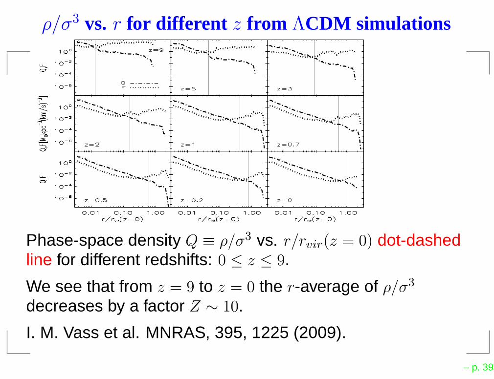
ρ/σ3 vs. r for different z from ΛCDM simulations

Phase-space density Q ≡ ρ/σ3 vs. r/rvir(z = 0) dot-dashedline for different redshifts: 0 ≤ z ≤ 9.

We see that from z = 9 to z = 0 the r-average of ρ/σ3

decreases by a factor Z ∼ 10.

I. M. Vass et al. MNRAS, 395, 1225 (2009).

– p. 39

Relics decoupling non-relativistic

FNRd (pc) = 2

52 π

72

45 gd Y∞(

Td

m

)

3

2 e− p2

c2 m Td = 2

52 π

72

45gd Y∞

x32

e−y2

2 x

Y (t) = n(t)/s(t), n(t) number of DM particles per unitvolume, s(t) entropy per unit volume, x ≡ m/Td, Td < m.

Y∞ = 1π

√

458

1√gd Td σ0 MPl

late time limit of Boltzmann.

σ0: thermally averaged total annihilation cross-section timesthe velocity.

From our previous general equations for m and gd:

m = 454 π2

ΩDM ρc

g T 3γ Y∞

= 0.748g Y∞

eV and m5

2 T3

2

d = 452 π2

1g gd Y∞

Z ρs

σ3s

Finally:√m Td = 1.47

(

Zgd

)1

3

keV

We used ρDM today and the decrease of the phase spacedensity by a factor Z.

– p. 40

Relics decoupling non-relativistic 2

Allowed ranges for m and Td.

m > Td > b eV where b > 1 or b≫ 1 for DM decoupling inthe RD era(

Zgd

)1

3

1.47 keV < m < 2.16b MeV

(

Zgd

)2

3

gd ≃ 3 for 1 eV < Td < 100 keV and 1 < Z < 103

1.02 keV < m < 104b MeV , Td < 10.2 keV.

Only using ρDM today (ignoring the phase space densityinformation) gives one equation with three unknowns:m, Td and σ0,

σ0 = 0.16 pbarng√gd

m

Tdhttp://pdg.lbl.gov

WIMPS with m = 100 GeV and Td = 5 GeV require Z ∼ 1023.

– p. 41

Exact Inflaton Dynamics: w(χ) = y32

(χ2 − 8

y)2

0

10

20

30

40

50

60

70

0 0.5 1 1.5 2 2.5 3 3.5 4

log a(τ) vs. τ

0

0.1

0.2

0.3

0.4

0.5

0.6

0.7

0.8

0 0.5 1 1.5 2 2.5 3 3.5 4

H(τ) vs. τ

– p. 42

Exact Inflaton Dynamics: w(χ) = y32

(χ2 − 8

y)2

-1

0

1

2

3

4

5

6

7

8

0 0.5 1 1.5 2 2.5 3 3.5 4

χ(τ) vs. τ

χ(τ) vs. τ

In these plots y = 1.26 and χmin =√

8y = 2.52.

We choose χ(0) = 0.73587, 12 N χ(0)2 = w(χ(0)) ,

=⇒ χ(0) = 12.624 which ensure Ntot ≃ 66.

We have here neglected spatial gradient terms:

(∇φ)2

2 a2(t)since a(t) grows exponentially during inflation.

– p. 43

Higher Order Inflaton PotentialsTill here we considered fourth degree inflaton potentials.Can higher order terms modify the physical results and theobservable predictions?

We systematically study the effects produced by higherorder terms (n > 4) in the inflationary potential on theobservables ns and r.All coefficients in the potential w become order one usingthe field χ within the Ginsburg-Landau approach:w(χ) = c0 − 1

2 χ2 +

∑∞n=2

cn

n χ2 n , cn = O(1) .

All r = r(ns) curves for double–well potentials of arbitraryhigh order fall inside a universal banana-shaped region B.Moreover, the r = r(ns) curves for double–well potentialseven for arbitrary positive higher order terms lie inside thebanana region B.C. Destri, H. J. de Vega, N. G. Sanchez, arXiv:0906.4102.

– p. 44

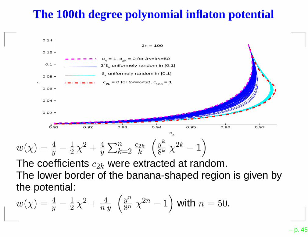
The 100th degree polynomial inflaton potential

0.91 0.92 0.93 0.94 0.95 0.96 0.970

0.02

0.04

0.06

0.08

0.1

0.12

0.14

ns

r2n = 100

c4 = 1, c

2k = 0 for 3<=k<=50

c2k

= 0 for 2<=k<50, c100

= 1

2kξk uniformely random in [0,1]

ξk uniformely random in [0,1]

w(χ) = 4y − 1

2 χ2 + 4

y

∑nk=2

c2k

k

(

yk

8k χ2k − 1

)

The coefficients c2k were extracted at random.The lower border of the banana-shaped region is given bythe potential:

w(χ) = 4y − 1

2 χ2 + 4

n y

(

yn

8n χ2n − 1)

with n = 50.

– p. 45

The inflaton potential from a fermion condensateInflaton coupled to Dirac fermions Ψ during inflation:

L = Ψ[

i γµ Dµ −mf − gY φ]

Ψ

gY = Yukawa coupling, γµ = curved space-time γ-matrices.Hubble parameter H = constant. Effective potential ≡fermions energy for a constant inflaton φ during inflation.Dynamically generated inflaton potential:

Vf (φ) = V0 + 12 µ

2 φ2 + 14 λ φ

4 +H4Q(

gYφH

)

, where

µ2 = −m2 < 0 mass squared, λ = quartic coupling,

Q(x) = x2

8 π2

(1 + x2) [γ + Reψ(1 + i x)] − ζ(3)x2

=

= x4

8 π2

[

(1 + x2)∑∞

n=1

1

n (n2 + x2)− ζ(3)

]

, x ≡ gYφH

Q(x)x→∞= x4

8 π2

[

log x+ γ − ζ(3) + O(

1x

)]

Minkowski limit (Coleman-Weinberg potential)

– p. 46

Effective fermionic inflaton potential and r vs.ns

0

0.2

0.4

0.6

0.8

1

1.2

0 0.2 0.4 0.6 0.8 1 1.2 1.4 1.6 1.8

0

0.02

0.04

0.06

0.08

0.1

0.12

0.14

0.92 0.925 0.93 0.935 0.94 0.945 0.95 0.955 0.96 0.965 0.97

y V (φ)/[8N M4] vs. φ/φmin for 0 < gY < 500 H/φmin

r vs. ns for 0 < gY < 800 H/φmin– p. 47

The universal banana region

0

0.02

0.04

0.06

0.08

0.1

0.12

0.14

0.92 0.93 0.94 0.95 0.96 0.97 0.98

We find that all r = r(ns) curves for double–well inflatonpotentials in the Ginsburg-Landau spirit fall inside theuniversal banana region B.The lower border of B corresponds to the limiting potential:

w(χ) = 4y − 1

2 χ2 for χ <

√

8y , w(χ) = +∞ for χ >

√

8y

This gives a lower bound for r for all potentials in theGinsburg-Landau class: r > 0.021 for the current best valueof the spectral index ns = 0.964.

– p. 48

The Energy Scale of Inflation

Grand Unification Idea (GUT)

Renormalization group running of electromagnetic,weak and strong couplings shows that they all meet atEGUT ≃ 2 × 1016 GeV

Neutrino masses are explained by the see-saw

mechanism: mν ∼ M2

Fermi

MRwith MR ∼ 1016 GeV.

Inflation energy scale: M ≃ 1016 GeV.

Conclusion: the GUT energy scale appears in at least threeindependent ways.

Moreover, moduli potentials: Vmoduli = M4SUSY v

(

φMPl

)

ressemble inflation potentials provided MSUSY ∼ 1016 GeV.First observation of SUSY in nature??

– p. 49

The number of efolds in Slow-roll

The number of e-folds N [χ] since the field χ exits thehorizon till the end of inflation is:

N [χ] = N∫ χχend

w(χ)w′(χ) dχ. We choose then N = N [χ].

The spontaneously broken symmetric potential:

w(χ) = y32

(

χ2 − 8y

)2

produces inflation with 0 <√y χinitial ≪ 1 and χend =

√

8y .

This is small field inflation.

From the above integral: y = z − 1 − log z

where z ≡ y χ2/8 and we have 0 < y <∞ for 1 > z > 0.Spectral index ns and the ratio r as functions of y:ns = 1 − y

N3 z+1(z−1)2 , r = 16 y

Nz

(z−1)2

– p. 50

Binomial New Inflation: ( y = coupling).r decreases monotonically with y :(strong coupling) 0 < r < 8

N = 0.16 (zero coupling).

-0.1

-0.05

0

0.05

0.1

0.15

0.2

0 0.5 1 1.5 2 2.5 3 3.5 4 4.5 5

(ns - 1) vs. y

r vs. y

ns first grows with y, reaches a maximum valuens,maximum = 0.96139 . . . at y = 0.2387 . . . and then ns

decreases monotonically with y.

– p. 51

Binomial New Inflation

0

0.02

0.04

0.06

0.08

0.1

0.12

0.14

0.16

0.93 0.935 0.94 0.945 0.95 0.955 0.96 0.965

r vs. ns

r = 8N = 0.16 and ns = 1 − 2

N = 0.96 at y = 0.

r is a double valued function of ns.

– p. 52

Quadrupole suppression and Fast-roll Inflation

The observed CMB-quadrupole (COBE,WMAP5) is sixtimes smaller than the ΛCDM model value.In the best ΛCDM fit the probability that the quadrupole isas low or lower than the observed value is 3%.It is hence relevant to find a cosmological explanation of thequadrupole suppression.

Generically, the classical evolution of the inflaton has a brieffast-roll stage that precedes the slow-roll regime.In case the quadrupole CMB mode leaves the horizonduring fast-roll, before slow-roll starts, we find that thequadrupole mode gets suppressed.

P (k) = |∆(S)k ad|2 (k/k0)

ns−1[1 +D(k)]

The transfer function D(k) changes the primordial power.1 +D(0) = 0, D(∞) = 0

– p. 53

The Fast-Roll Transfer Function

0

0.2

0.4

0.6

0.8

1

1.2

1.4

0 10 20 30 40 50 60 70 80 90 100

D(k) vs. k/m

kQ = 11.5 m, kfastroll→slowroll = 14 m, kpivot = 96.7 m,

m = 1.21 1013GeV, ktodayQ = 0.238 Gpc−1 =⇒ redshift at the

beginning of inflation = 0.9 × 1056 ≃ e129.– p. 54

Comparison, with the experimental WMAP5 dataof the theoretical CTT

ℓ multipoles

0.5 1 1.5 2 2.5 3 3.5 4 4.5 5 5.50

1000

2000

3000

4000

5000

6000

7000

log(multipole index)

l(l+1

)Cl/2

π

2 3 4 5 6 7 8

200

400

600

800

1000

1200

1400WMAP5 data

ΛCDM+r

BNI+sharpcut

BNI+fastroll

– p. 55

Comparison, with the experimental WMAP5 dataof the theoretical CTE

ℓ multipoles

0.5 1 1.5 2 2.5 3 3.5

−15

−10

−5

0

5

10

15

20

log(multipole index)

l(l+1

)Cl/2

π

WMAP5 data

ΛCDM+r

BNI+sharpcut

BNI+fastroll

– p. 56

Comparison, with the experimental WMAP-5 dataof the theoretical CEE

ℓ multipoles

2 3 4 5 6 7

0

0.1

0.2

0.3

0.4

0.5

multipole index l

l(l+1

)Cl/2

π

WMAP5 dataΛCDM+rBNI+sharpcutBNI+fastroll

– p. 57

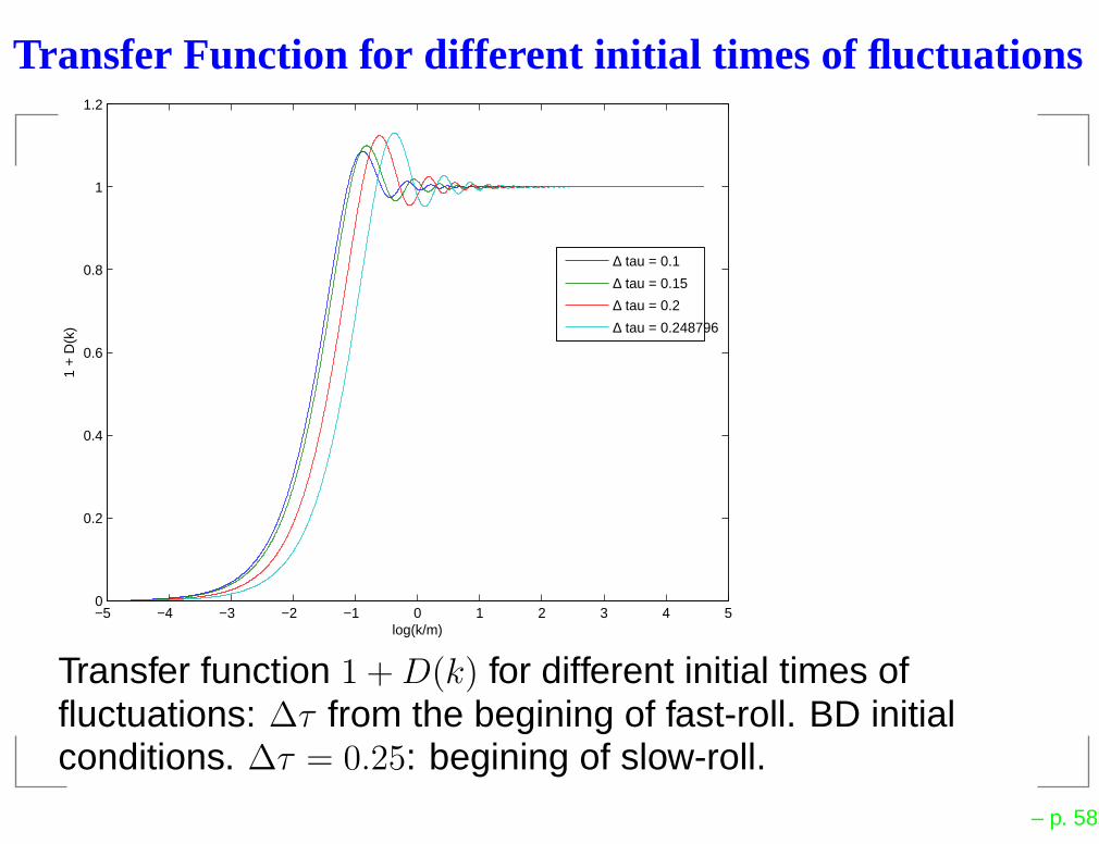
Transfer Function for different initial times of fluctuations

−5 −4 −3 −2 −1 0 1 2 3 4 50

0.2

0.4

0.6

0.8

1

1.2

log(k/m)

1 +

D(k

)

∆ tau = 0.1

∆ tau = 0.15

∆ tau = 0.2

∆ tau = 0.248796

Transfer function 1 +D(k) for different initial times offluctuations: ∆τ from the begining of fast-roll. BD initialconditions. ∆τ = 0.25: begining of slow-roll.

– p. 58

∆CTT

ℓ vs. initial time of fluctuations

-1

-0.8

-0.6

-0.4

-0.2

0

0.2

0.4

0 0.05 0.1 0.15 0.2 0.25

∆C1 vs. ∆τ∆C2 vs. ∆τ∆C3 vs. ∆τ

Changes on the dipole, quadrupole and octupoleamplitudes according to the starting time ∆τ chosen for thefluctuations from the begining of fast-roll. BD initialconditions. ∆τ = 0.25: begining of slow-roll.

– p. 59

Loop Quantum Corrections to Slow-Roll Inflation

φ(~x, t) = Φ0(t)+ϕ(~x, t), Φ0(t) ≡< φ(~x, t) >, < ϕ(~x, t) >= 0

ϕ(~x, t) = 1a(η)

∫

d3k(2 π)3

[

a~kχk(η) e

i~k·~x + h.c.]

,

a†~k, a~k

are creation/annihilation operators,

χk(η) are mode functions. η = conformal time.To one loop order the equation of motion for the inflaton is

Φ0(t) + 3H Φ0(t) + V ′(Φ0) + g(Φ0) 〈[ϕ(x, t)]2〉 = 0

where g(Φ0) = 12 V

′′′

(Φ0).The mode functions obey:

χ′′

k(η) +

[

k2 +M2(Φ0) a2(η) − a

′′

(η)a(η)

]

χk(η) = 0

where M2(Φ0) = V ′′(Φ0) = 3 H20 ηV + O(1/N2)

– p. 60

Quantum Corrections to the Friedmann Equation

The mode functions equations for slow-roll become,

χ′′

k(η)+[

k2 − ν2− 1

4

η2

]

χk(η) = 0 , ν = 32 + ǫV −ηV +O(1/N2).

The scale factor during slow roll is a(η) = − 1H0 η (1−ǫV ) .

Scale invariant case: ν = 32 . ∆ ≡ 3

2 − ν = ηV − ǫV controlsthe departure from scale invariance.Explicit solutions in slow-roll:

χk(η) = 12

√−πη iν+ 1

2 H(1)ν (−kη), H

(1)ν (z) = Hankel function

Quantum fluctuations: 〈[ϕ(x, t)]2〉 = 1a2(η)

∫

d3k(2π)3 |χk(η)|2

12〈[ϕ(x, t)]2〉 =

(

H0

4 π

)2 [Λp

2 + ln Λ2p + 1

∆ + 2 γ − 4 + O(∆)]

UV cutoff Λp = physical cutoff/H, 1∆ = infrared pole.

⟨

ϕ2⟩

,⟨

(∇ϕ)2⟩

are infrared finite

– p. 61

Quantum Corrections to the Inflaton Potential

Upon UV renormalization the Friedmann equation results

H2 = 13 M2

Pl

[

12 Φ0

2+ VR(Φ0) +

(

H0

4 π

)2 V′′

R (Φ0)∆ + O

(

1N

)

]

Quantum corrections are proportional to(

HMPl

)2∼ 10−9 !!

The Friedmann equation gives for the effective potential:

Veff (Φ0) = VR(Φ0) +(

H0

4 π

)2 V′′

R (Φ0)∆

Veff (Φ0) = VR(Φ0)

[

1 +(

H0

4 π MPl

)2ηV

ηV −ǫV

]

in terms of slow-roll parameters

Very DIFFERENT from the one-loop effective potential inMinkowski space-time:

Veff (Φ0) = VR(Φ0) + [V′′

R (Φ0)]2

64 π2 ln V′′

R (Φ0)M2

– p. 62

Quantum Fluctuations:Scalar Curvature, Tensor, Fermion, Light Scalar.All these quantum fluctuations contribute to the inflatonpotential and to the primordial power spectra.

In de Sitter space-time: < Tµ ν >= 14 gµ ν < Tα

α >

Hence, Veff = VR+ < T 00 >= VR + 1

4 < Tαα >

Sub-horizon (Ultraviolet) contributions appear through thetrace anomaly and only depend on the spin of the particle.Superhorizon (Infrared) contributions are of the order N0

and can be expressed in terms of the slow-roll parameters.

Veff (Φ0) = V (Φ0)

[

1 + H20

3 (4π)2 M2

Pl

(

ηv−4 ǫv

ηv−3 ǫv+ 3 ησ

ησ−ǫv+ T

)]

T = TΦ + Ts + Tt + TF = −290320 is the total trace anomaly.

TΦ = Ts = −2930 , Tt = −717

5 , TF = 1160

−→ the graviton (t) dominates.– p. 63

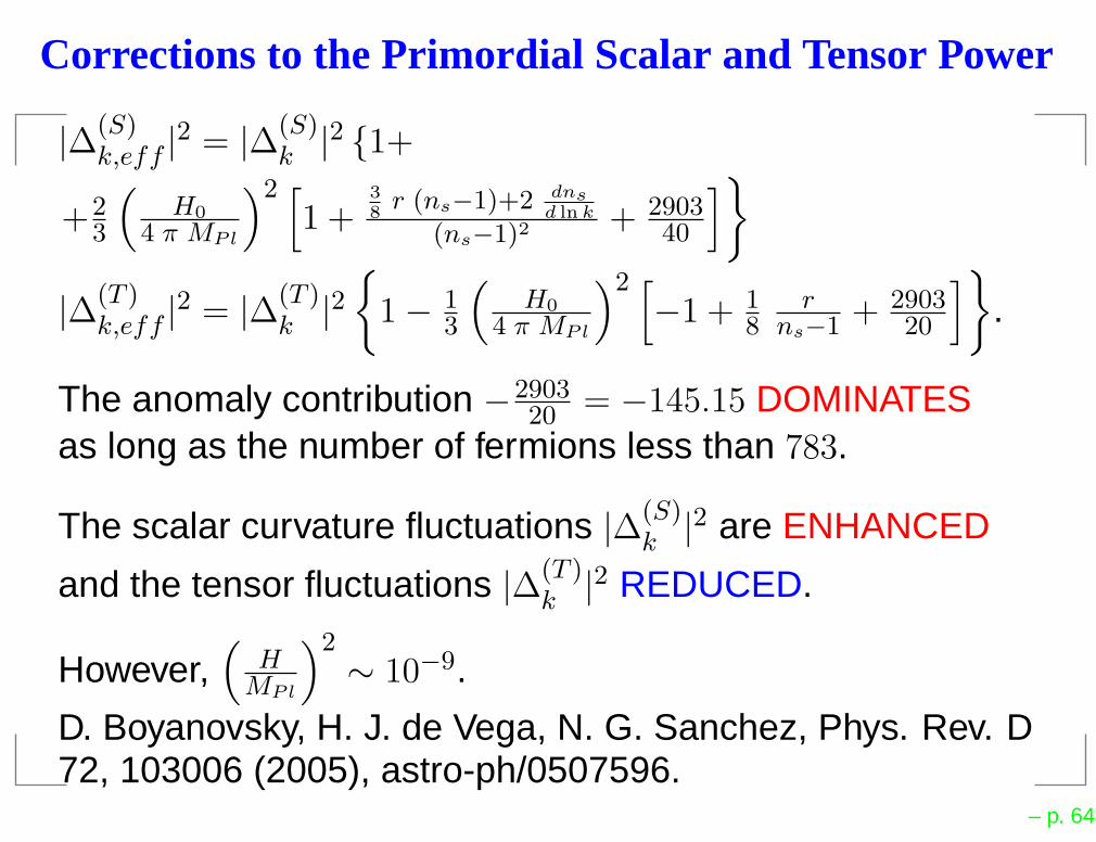
Corrections to the Primordial Scalar and Tensor Power

|∆(S)k,eff |2 = |∆(S)

k |2 1+

+23

(

H0

4 π MPl

)2 [

1 +3

8r (ns−1)+2 dns

d ln k

(ns−1)2 + 290340

]

|∆(T )k,eff |2 = |∆(T )

k |2

1 − 13

(

H0

4 π MPl

)2 [

−1 + 18

rns−1 + 2903

20

]

.

The anomaly contribution −290320 = −145.15 DOMINATES

as long as the number of fermions less than 783.

The scalar curvature fluctuations |∆(S)k |2 are ENHANCED

and the tensor fluctuations |∆(T )k |2 REDUCED.

However,(

HMPl

)2∼ 10−9.

D. Boyanovsky, H. J. de Vega, N. G. Sanchez, Phys. Rev. D72, 103006 (2005), astro-ph/0507596.

– p. 64

Linear results for µ0D and the profile vs. observations

Since the surface density r0 ρ(0) should be universal, wecan identify rlin ρlin(0) from a spherically symmetric solutionof the linearized Boltzmann-Vlasov equation.

The comparison of our theoretical values for µ0D and theobservational value indicates that Z ∼ 10 − 1000. Recallingthe DM particle mass:

m = 0.568(

Zg

)1

4

keV for Fermions.

This implies that the DM particle mass is in the keV range.

Remarks:1) For larger scales nonlinear effects from small k shouldgive the customary r−3 tail in the density profile.2) The linear approximation describe the limit of very largegalaxies with typical inner size rlin ∼ 100 kpc.

– p. 65