The Effect of Zoning on Housing Prices - Amazon S3 · Phone: +61 2 9551 9830 Facsimile: +61 2 9551...

The Effect of Zoning on Housing Prices

Ross Kendall and Peter Tulip

Research Discussion Paper

R D P 2018- 03

Figures in this publication were generated using Mathematica.

The contents of this publication shall not be reproduced, sold or distributed without the prior consent of the Reserve Bank of Australia and, where applicable, the prior consent of the external source concerned. Requests for consent should be sent to the Secretary of the Bank at the email address shown above.

ISSN 1448-5109 (Online)

The Discussion Paper series is intended to make the results of the current economic research within the Reserve Bank available to other economists. Its aim is to present preliminary results of research so as to encourage discussion and comment. Views expressed in this paper are those of the authors and not necessarily those of the Reserve Bank. Use of any results from this paper should clearly attribute the work to the authors and not to the Reserve Bank of Australia.

Enquiries:

Phone: +61 2 9551 9830 Facsimile: +61 2 9551 8033 Email: [email protected] Website: http://www.rba.gov.au

The Effect of Zoning on Housing Prices

Ross Kendall and Peter Tulip

Research Discussion Paper 2018-03

March 2018

Economic Research Department Reserve Bank of Australia

The authors would like to thank Paul Chudleigh, Brendan Coates, Luci Ellis, Jonathan Kearns,

Gianni La Cava, Kirdan Lees, Phil Manners, David Norman, Anthony Richards, Tom Rosewall,

John Simon, Trent Wiltshire and seminar participants at the Reserve Bank of Australia, New South

Wales Department of Planning and Environment, and New South Wales Treasury for useful

feedback and discussions. The RBA’s Regional and Industry Analysis section provided valuable

assistance. The views expressed in this paper are those of the authors and do not necessarily

reflect the views of the Reserve Bank of Australia. The authors are solely responsible for any

errors.

An additional Online Appendix, Stata programs and data are available at

<https://www.rba.gov.au/publications/rdp/2018/2018-03/supplementary-information.html>.

Author: tulipp at domain rba.gov.au

Media Office: [email protected]

Abstract

Zoning regulations provide benefits, but they also restrict housing supply and hence raise prices.

This paper quantifies their importance by comparing prices to the marginal costs of supply at

different points in time. For detached houses, marginal costs comprise the dwelling structure and

the land that other home owners need to forego. Relative to our estimates of these costs, we find

that, as of 2016, zoning raised detached house prices 73 per cent above marginal costs in Sydney,

69 per cent in Melbourne, 42 per cent in Brisbane and 54 per cent in Perth. Zoning has also raised

the price of apartments well above the marginal cost of supply, especially in Sydney. We

emphasise that this is not the amount that housing prices would fall in the absence of zoning. The

effect of zoning has increased dramatically over the past two decades, likely due to existing

restrictions binding more tightly as demand has risen.

JEL Classification Numbers: R31, R52

Keywords: housing, housing prices, land prices, zoning, land use

Table of Contents

1. Introduction 1

2. Related Research 3

3. Decomposing Property Values into Dwelling Structure and Land 4

4. Estimating the Physical Value of Land 8

5. Zoning Effect Estimates 10

5.1 Robustness of Our Hedonic Estimates 12

5.2 Sensitivity of Our Zoning Effect Estimates to Inputs 13

5.3 Other Issues 14

6. Decomposing Average House Prices over Time 15

7. Geographic Distribution of Zoning Effects within Cities 16

8. Apartment Prices and Marginal Costs 19

9. Discussion 22

Appendix A : Examples of Zoning Effects on Land and Property Values 24

Appendix B : Detailed 2016 Detached Housing Regression Results 25

References 29

Copyright and Disclaimer Notices 34

1. Introduction

Some government policies, which we will refer to as zoning, restrict the supply of housing.

Examples include minimum lot sizes, maximum building heights and planning approval processes.

Although these restrictions may confer benefits, they also raise the price of housing. This paper

attempts to quantify the effect of zoning on housing prices in Australia’s four largest cities.

Anecdotal evidence suggests that zoning can have a huge effect on land values. For example, a

363 hectare site in Wyndam Vale (40 km west of Melbourne) increased in value from $120 million

to $400 million following its rezoning from rural to residential (Schlesinger and Tan 2017).

Examples like this are common – Appendix A provides more. Such large increases in values as a

result of zoning changes are inconsistent with the view that a physical shortage of land itself is the

main cause of high land values and housing prices – and instead point towards a high ‘shadow

price’ of government permission to build dwellings as a likely explanation. It is difficult, however,

to gauge how representative these anecdotes are, or to analyse how they change over time or

place.

A natural approach to this issue might be to examine the effects of differences in zoning

regulations. However, for reasons we discuss in Section 2, that approach is not appropriate for

estimating zoning’s overall effect on prices. Instead, we follow the approach of Glaeser and

Gyourko (2003) and Glaeser, Gyourko and Saks (2005), which involves comparing property prices

to the marginal cost of supply. For detached houses, this means decomposing property values into

the cost of the structure and the value of physical land at that location, with the remainder being

attributable to zoning restrictions.

To illustrate, and to preview our results, we estimate that the average Sydney house, valued at

$1.16 million in 2016, represents a $395 000 structure on a $765 000 block of land.1 However, the

reason land is expensive is not because it is physically scarce. Hedonic regressions indicate that

home owners do not value it, as land, especially highly. Specifically, they value land as worth

about $400 a square metre on the margin, or $277 000 for the average Sydney block. This

‘marginal’ or ‘physical’ value of land represents the opportunity cost of extra land, as judged by

what people are prepared to pay for it.2 This is $489 000 less than its market value. This

difference represents what home owners need to pay for the right to have a dwelling at that

location, or the cost of ‘administrative’ scarcity. The academic literature refers to this difference as

the ‘zoning tax’ because the wedge between prices and costs is induced by government-

determined scarcity and to draw an analogy with a Pigouvian welfare tax. We, however, use the

less-loaded term ‘zoning effect’, which avoids implying that government revenue is involved.

The difference between the average (or market) price and the marginal (or physical) value of land

represents an arbitrage opportunity. In the absence of zoning, an investor could purchase

properties where the marginal value of land is lower than the average value, subdivide them to

create multiple smaller properties, and make a profit. More concretely, excluding the effect of

1 To provide context for international readers, the mean annual household disposable income in Australia was $97 000

in 2015/16 (based on the ABS Survey of Income and Housing). Fox and Finlay (2012) discuss internationally

consistent comparisons of housing prices and incomes.

2 Although the value of physical land is low relative to the sale price, it is high in Sydney relative to other Australian

cities. Moreover, physical land values in Australian cities are higher than in some overseas cities, a point we discuss

in Section 4.

2

zoning, the marginal Sydney house buyer could have been supplied with an average house for

$671 000 – it would have cost $395 000 to build the structure and landowners (existing or

potential) would have been prepared to forego the land for $277 000. Instead, buyers needed to

pay $1.16 million. The extra $489 000 reflects administrative restrictions. That is, zoning

restrictions raised prices 73 per cent above the cost of supply.

This effect is similar but smaller in other cities. We estimate that zoning restrictions raised the

average price of detached houses, relative to supply costs, by 69 per cent in Melbourne, 42 per

cent in Brisbane and 54 per cent in Perth. As a share of the total price, these contributions are

42 per cent (Sydney), 41 per cent (Melbourne), 29 per cent (Brisbane) and 35 per cent (Perth).

Higher-density dwellings require a slightly different approach. As discussed in Section 8, we

estimate that zoning restrictions raised average apartment prices, relative to marginal cost, by

85 per cent in Sydney, 30 per cent in Melbourne and 26 per cent in Brisbane.

Figure 1, a standard supply-demand diagram, may help to interpret our estimates. Point A

represents a frictionless market, with the number of dwellings equal to QE supplied and demanded

at price PE. However, if restrictions limit supply to QMax, the price would rise to PZoning as QMax

intersects the demand curve at point B. The gap between what home buyers pay (PZoning) and the

marginal cost of supply (PSupply) is our estimate of the zoning effect. This zoning effect or ‘shadow

price’ can be thought of as the price a developer would be willing to pay for permission to build

one more dwelling at a given location.

Figure 1: Stylised Housing Market with a Binding Quantitative Zoning Constraint

As this diagram indicates, our focus is narrow and partial equilibrium in nature: specifically, we

focus on the effect of zoning on prices under current conditions. While this allows us to answer

some important questions about the effect of zoning regulations, there are others that we cannot

address. In particular, we do not examine effects on quantities, incomes or other measures. Nor

do we examine the benefits of zoning, such as the externalities of congestion and

Price

Number of

dwellings

Supply

Demand

QMax

Zoning

effect

A

B

QE

PSupply

PZoning

PE

3

overdevelopment. Our approach does not allow us to estimate the difference in house prices

compared with a counterfactual of no zoning restrictions (PE in Figure 1). Estimating this difference

would require estimating the slope of demand and supply curves, together with general

equilibrium effects. This would be an important exercise for a calculation of welfare costs, but it is

beyond the scope of this paper. Kulish, Richards and Gillitzer (2011) address this issue.

Another limitation of our approach is that because we estimate the effect of zoning indirectly, as a

residual, any errors in our estimates of the other components of marginal costs will flow through

to our estimated zoning effect. This matters because our estimates of costs rest on some

assumptions that strike us as reasonable, but are difficult to quantify.

2. Related Research

Several government, academic and private sector studies have pointed to restrictive zoning as

being an important factor in Australia’s high and rising housing prices. These include OECD (2010);

Kulish et al (2011); Productivity Commission (2011, 2017); HSAR Working Party (2012);

RBA (2014); Senate Economics References Committee (2015); CEDA (2017); Stevens (2017) and

Daley, Coates and Wiltshire (2018), among others. Most of those papers that make policy

recommendations call for increases in land supply and changes to zoning rules to allow for greater

housing density. A problem with that recommendation is that it implicitly weighs benefits against

costs, but these are not based on quantitative evidence. This paper tries to partially fill that gap by

quantifying the effect of zoning restrictions on housing prices.

Several previous studies have focused on variations in zoning regulations. McIntosh, Trubka and

Hendriks (2016, p 52) regress Sydney land values on zoning regulations and numerous other

controls, including suburb and distance to transport. They find that rezoning a property from

detached housing (a floor space to land area ratio of 0.5) to a 5- to 10-storey apartment block (a

floor space to land area ratio of 4) would, on average, increase the value of land by 167 per cent.

In an earlier, simpler study, the Centre for International Economics (CIE and ARUP 2012;

CIE 2013) finds effects from a number of different types of zoning restrictions. In total, these

restrictions are conservatively estimated as imposing a cost of $8 to $16 billion in Sydney, which is

small relative to the value of the housing stock. There have been many international studies of

variations in regulations; these often find large effects on prices. Gyourko and Molloy (2015),

Furman (2015) and Hilber and Vermeulen (2016) provide overviews of this research.

In contrast, Ong et al (2017) examine variations in the number and types of planning controls

used by local councils and find they have little effect on housing supply. This may be because, as

they discuss (p 50), their planning controls do not reflect variations in zoning or density measures.

Instead, their estimates place substantial weight on the number of controls used, including a

variety of controls that we would not expect to have a material effect on supply or prices – for

example, relating to caravan parks, native vegetation and so on.

In addition to study-specific issues, there are some general limitations with a focus on variations in

regulations. First, most of the papers cited above estimate the effects of differences in regulations,

whereas we are interested in their overall effect. It is often not the variations in zoning that

matter, but their average level. As Kulish et al (2011) discuss, a uniform restriction (for example, a

height limit) will have a much larger effect in the city centre than in outlying suburbs. And

4

unchanged restrictions will bind more tightly as demand grows. Second, regulations vary from one

jurisdiction to the next, which makes it difficult to compare, aggregate or extend estimates. Third,

variations in zoning are often a function of variations in prices, as well as a cause, an issue

emphasised by Saiz (2010).

In their literature survey, Gyourko and Molloy (2015) suggest that these difficulties can be avoided

by comparing prices to the marginal cost of supply. This is the approach taken by Glaeser and

Gyourko (2003) and Glaeser et al (2005), who examine single-family detached dwellings in

US metropolitan areas. They find that the wedge between marginal costs and prices is large in

markets where narrative evidence suggests zoning restrictions bind tightly (typically big coastal

cities) and negligible in others where restrictions are thought to be loose, such as in the south and

mid-west. We discuss this approach and apply it to Australia’s largest cities in Sections 3, 4 and 5.

Others have already applied this approach elsewhere. Lees (2018) studies cities in New Zealand.

Cheung, Ihlanfeldt and Mayock (2009) look at metropolitan areas in Florida and Sunding and

Swoboda (2010) examine southern California. In an undergraduate essay, Turnbull (2005)

examines the Sydney housing market. These studies all find large effects of zoning for some cities.

As we discuss below, we have better data than was available to these researchers. Nevertheless,

our estimates are similar.

High-density housing raises different issues and calls for a slightly modified approach. Glaeser

et al (2005) compare the market price of apartments in Manhattan to the marginal cost of adding

an additional floor to a development. They find a large gap between prices and marginal cost,

from which they conclude that regulatory restrictions were responsible for at least half of the price

of apartments in Manhattan in the early 2000s. Cheshire and Hilber (2008) apply this approach to

commercial property in Europe and find that restrictions on supply increase office rents several

fold. We apply this approach to Australia in Section 8.

3. Decomposing Property Values into Dwelling Structure and Land

To estimate the effect of zoning, we consider the cost of a marginal increase in the number and

density of dwellings for a given area and given population (hence a reduction in average

household size). This means that we do not include the costs involved in increasing the footprint

or size of a city, such as provision of extra roads and utilities, as a cost of supplying housing.

We first decompose property values into contributions from land and structures. We have three

main sources of information on this, each of which gives broadly similar results (Table 1). Readers

who are not interested in the strengths and limitations or calculation of the various measures can

take our baseline estimates as given and skip ahead to the next section. Further details are in the

Online Appendix (Section 1), available in the supplementary information provided with this paper

on the RBA’s website.

Perhaps the simplest and most direct approach to splitting land and structure values is to use

estimates of land values from state valuers general, who collect estimates for tax purposes. In

Australia, land taxes are levied by state and (especially) local governments. These estimates are

constructed using sales of vacant lots and improved properties, with the latter adjusted to remove

the value of the improvements.

5

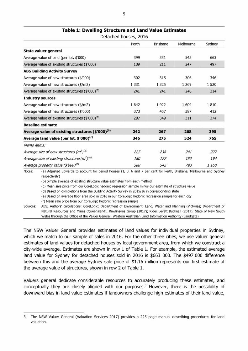
Table 1: Dwelling Structure and Land Value Estimates

Detached houses, 2016

Perth Brisbane Melbourne Sydney

State valuer general

Average value of land (per lot, $’000) 399 331 545 663

Average value of existing structures ($’000) 189 211 247 497

ABS Building Activity Survey

Average value of new structures ($’000) 302 315 306 346

Average value of new structures ($/m2) 1 331 1 325 1 269 1 520

Average value of existing structures ($’000)(a) 241 241 246 314

Industry sources

Average value of new structures ($/m2) 1 642 1 922 1 604 1 810

Average value of new structures ($’000) 373 457 387 412

Average value of existing structures ($’000)(a) 297 349 311 374

Baseline estimate

Average value of existing structures ($’000)(b) 242 267 268 395

Average land value (per lot, $’000)(c) 346 275 524 765

Memo items:

Average size of new structures (m2) (d) 227 238 241 227

Average size of existing structures(m2) (e) 180 177 183 194

Average property value ($’000) (f) 588 542 793 1 160

Notes: (a) Adjusted upwards to account for period houses (1, 3, 6 and 7 per cent for Perth, Brisbane, Melbourne and Sydney

respectively)

(b) Simple average of existing structure value estimates from each method

(c) Mean sale price from our CoreLogic hedonic regression sample minus our estimate of structure value

(d) Based on completions from the Building Activity Survey in 2015/16 in corresponding state

(e) Based on average floor area sold in 2016 in our CoreLogic hedonic regression sample for each city

(f) Mean sale price from our CoreLogic hedonic regression sample

Sources: ABS; Authors’ calculations; CoreLogic; Department of Environment, Land, Water and Planning (Victoria); Department of

Natural Resources and Mines (Queensland); Rawlinsons Group (2017); Rider Levett Bucknall (2017); State of New South

Wales through the Office of the Valuer General; Western Australian Land Information Authority (Landgate)

The NSW Valuer General provides estimates of land values for individual properties in Sydney,

which we match to our sample of sales in 2016. For the other three cities, we use valuer general

estimates of land values for detached houses by local government area, from which we construct a

city-wide average. Estimates are shown in row 1 of Table 1. For example, the estimated average

land value for Sydney for detached houses sold in 2016 is $663 000. The $497 000 difference

between this and the average Sydney sale price of $1.16 million represents our first estimate of

the average value of structures, shown in row 2 of Table 1.

Valuers general dedicate considerable resources to accurately producing these estimates, and

conceptually they are closely aligned with our purposes.3 However, there is the possibility of

downward bias in land value estimates if landowners challenge high estimates of their land value,

3 The NSW Valuer General (Valuation Services 2017) provides a 225 page manual describing procedures for land

valuation.

6

but not low estimates.4 Anecdotal reports suggest this bias may be significant. In addition, there

are likely to be some small differences in how the estimates are constructed in different states.

One advantage of the valuer general estimates is that they are disaggregated by local government

area, which we examine in Section 7.

The ABS’s Building Activity Survey (BAS) provides estimates of the value of new detached dwelling

structures by state. For example, as shown in row 3 of Table 1, our estimate from the BAS of the

average cost of building a new house in NSW in 2016 was $346 000.5 However, we need estimates

of the value of existing structures, which will tend to be smaller than the value of new structures,

given that house size has increased over time. We account for this by adjusting construction costs

in proportion. The average house built in NSW in 2016 was 227 square metres, implying an

average construction cost of $1 520 per square metre (row 4). We multiply this construction cost

by the average floor space of existing houses (194 square metres) and add a 7 per cent upward

adjustment for period houses (discussed in the Online Appendix) to estimate the value of existing

house structures of about $314 000 (row 5).

A third source of information on construction costs is provided by Rawlinsons Construction Cost

Guide (Rawlinsons Group 2017) and Rider Levett Bucknall’s (RLB) ‘Riders Digest 2017’ (Rider

Levett Bucknall 2017). These are widely used references in the construction industry that provide

estimates for different types of construction projects in different cities. Rawlinsons and RLB report

estimates on a cost per square metre basis. As shown in row 6, our estimates from these sources

suggest that in Sydney a new house would cost $1 810 per square metre to build. As shown in

row 7, this would imply that a new Sydney house would cost $412 000 to build, while replacing the

average established Sydney house with one the same size would cost $374 000 (row 8). This

method is similar to the approach used by Glaeser et al (2005), who use industry-sourced

estimates of construction costs to derive estimates of structure value.

Two difficulties in inferring the value of existing dwellings from new construction costs are allowing

for depreciation and renovations and dealing with ‘period houses’. We discuss these in the Online

Appendix, Section 1.

The three estimates of construction costs discussed above each have their strengths and

weaknesses. However, for our purposes the similarity of the estimates is more important. They

range from 27 per cent to 43 per cent of the average Sydney sale price, from 31 to 39 per cent for

Melbourne, from 39 to 64 per cent for Brisbane, and from 32 to 51 per cent for Perth. None of the

three approaches consistently generates the highest or the lowest estimate. Our estimates contain

some outliers. For example, the structure value in Sydney based on valuer general estimates is

high relative to other cities and other approaches. The industry-based structure estimate in

Brisbane is high relative to the other estimates. We expect that closer examination of the

underlying data would narrow these ranges, but this would have little effect on our conclusions

and is left for further work.

4 A 2005 report (NSW Ombudsman 2005) documented cases of conservative valuations being applied in some areas,

but these issues may have since been addressed.

5 Industry sources suggest that construction costs are typically higher outside of capital cities. Building approvals data

are available at a more disaggregated regional level, but are likely to be more volatile (Hodges 2015).

7

For purposes of a baseline, we take a simple average of the structure value estimates from each

method, shown in Table 1. For Sydney, this means an average structure cost of $395 000 and an

average land value of $765 000 given the average sale price of $1.16 million.

The estimates in Table 1 can be compared with other estimates. The annual national accounts

estimate that the value of residential land in Australia is approximately twice the value of

residential dwelling structures. This is similar to the results in Table 1. Unfortunately, however, the

national accounts estimates do not distinguish between detached and high-density dwellings.

Moreover, estimates are available at the state but not city level. That said, these data can be

useful for evaluating national trends (e.g. Lowe 2015).

The UDIA (2017) report that vacant lots of land sold for an average of $465 000 in Sydney and

$237 000 in Melbourne in 2016. These estimates are far below the prices of land in Table 1. This is

because most undeveloped land is located on the outskirts of cities and these vacant lots tend to

be relatively small.

Urbis (2011) estimates development costs for detached housing on greenfield sites and for

apartment blocks on infill sites. These estimates have been emphasised by Hsieh, Norman and

Orsmond (2012) and RBA (2014). After allowing for inflation and differences in house size, the

Urbis construction cost estimates for detached housing are similar to those in Table 1, which is

unsurprising given that they are sourced from Rider Levett Bucknall. Urbis estimates of land costs

for detached housing are much lower, reflecting their focus on greenfield developments in outlying

suburbs (and the rapid growth in land prices subsequent to their study).

Urbis make explicit allowance for some additional costs that we exclude, most importantly

subdivision and infrastructure costs. This reflects their different focus. Whereas they are interested

in the cost of converting more land to residential use, we are interested in more intensive use of

residential land that is already serviced.6 A liberalisation of zoning would not directly increase the

population or area of a city, so the costs of urban growth are appropriately excluded from our

estimates of marginal cost.7 In any case, these costs are not large, relative to our estimates, and

would not change our conclusions. An upper bound on these costs is provided by Urbis’s estimates

of average costs per dwelling for Sydney greenfield sites: subdivision construction costs were

estimated at $47 000 and infrastructure costs (including Section 94 contributions) were $44 000 in

2011. Together these amounted to about 13 per cent of the average Sydney sale price. The

Housing Industry Association (2011) and Centre for International Economics (CIE 2011) argue that

a large part of the ‘infrastructure charge’ does not reflect genuine costs. These costs are much

lower on infill sites and in other cities. The Online Appendix (Section 1) discusses these costs and

charges in more detail.

6 In technical terms, they hold density or factor proportions constant and vary the scale of production. For an

examination of the effect of zoning, it is appropriate to hold the scale constant and vary density.

7 Of course, increased housing supply in one locality would encourage migration to that area. But changes in zoning

policy would not directly affect national population so there would be offsetting infrastructure savings elsewhere. For

a given population, average infrastructure costs often decrease as density rises, in which case these ‘costs’ would be

negative.

8

4. Estimating the Physical Value of Land

Having estimated that property prices (particularly in Sydney and Melbourne) largely reflect the

high value of land, we turn to the question of why land is so expensive. Our results in this section

indicate that home buyers are not prepared to pay an especially large amount for additional land –

suggesting that land’s scarcity as a physical commodity (at that location) does not account for the

high prices we observe. This can be seen from a hedonic regression of house sale prices as

follows.

log logsale price c b land area a e X

Our focus is on the coefficient b, which represents the marginal value of land (sometimes called

the ‘intensive margin’ or the value of physical land), while c is a constant, X is a vector of controls

for other characteristics of each property, such as location, number of bedrooms, number of

bathrooms and so on and e is a residual. We emphasise that what we call the value of physical

land is location-specific, and should be interpreted as what home buyers are prepared to pay for

an additional piece of land at a given location. The log-log specification means that physical land is

more expensive, on the margin, in locations where prices are high.8

We estimate our equation using unit record data of residential property sales. The data are

available for purchase from CoreLogic and are discussed in the Online Appendix (Section 2). In

brief, we restrict our sample to detached dwellings, and include only the most recent sale of each

property. We allocate property sales according to the Greater Capital City Statistical Areas defined

by the ABS, which correspond to a very broad area around each city. For example, our Sydney

sample extends to the Blue Mountains and Gosford. Our Melbourne sample includes the

Mornington Peninsula and Mitchell. Before estimating our equations, we make a number of

adjustments to clean the data and remove outliers.9

Our regressions control for local geographic characteristics using dummies corresponding to the

suburb of each property as provided by CoreLogic. As might be expected, these controls account

for a large proportion of the variance in sale prices.10 We also include quarterly time dummies. We

report standard errors allowing for clustering at the local government area level, as there may be

geographical correlation within the model residuals due to regional characteristics that we do not

control for. White standard errors are much smaller.

We report the results of regressions including different sets of additional control variables. Our

small regression includes only a small number of property characteristics that are likely to be the

most important, are commonly used in the hedonic house price literature, and have few or no

missing values in our sample. Our medium regression includes a number of extra control variables

which have few or no missing values in our sample and category dummies in place of the number

of bedrooms and bathrooms. Our large regression includes additional control variables for which

8 We will later demonstrate that our results are robust to a range of plausible alternative hedonic regression

specifications.

9 For example, we exclude houses with more than 2 acres of land in line with Glaeser et al (2005) in order to reduce a

possible source of downward bias in our hedonic estimate of land value.

10 Hill and Scholz (2014) find postcode dummies can account for the vast majority of geospatial variance in the data,

due to the relatively narrow definition of postcodes in Australian cities. We use CoreLogic’s suburb classifications,

which are more narrowly defined than postcodes, but this choice has minimal quantitive effect on our results.

9

we do not have data for a substantial portion of our observations. Rather than excluding

observations which have missing values for one of these extra variables (around half in 2016, and

substantially more for earlier years), we include an indicator dummy for whether an observation

has a value recorded or not to control for potential compositional differences between sales with

more or less information recorded.11

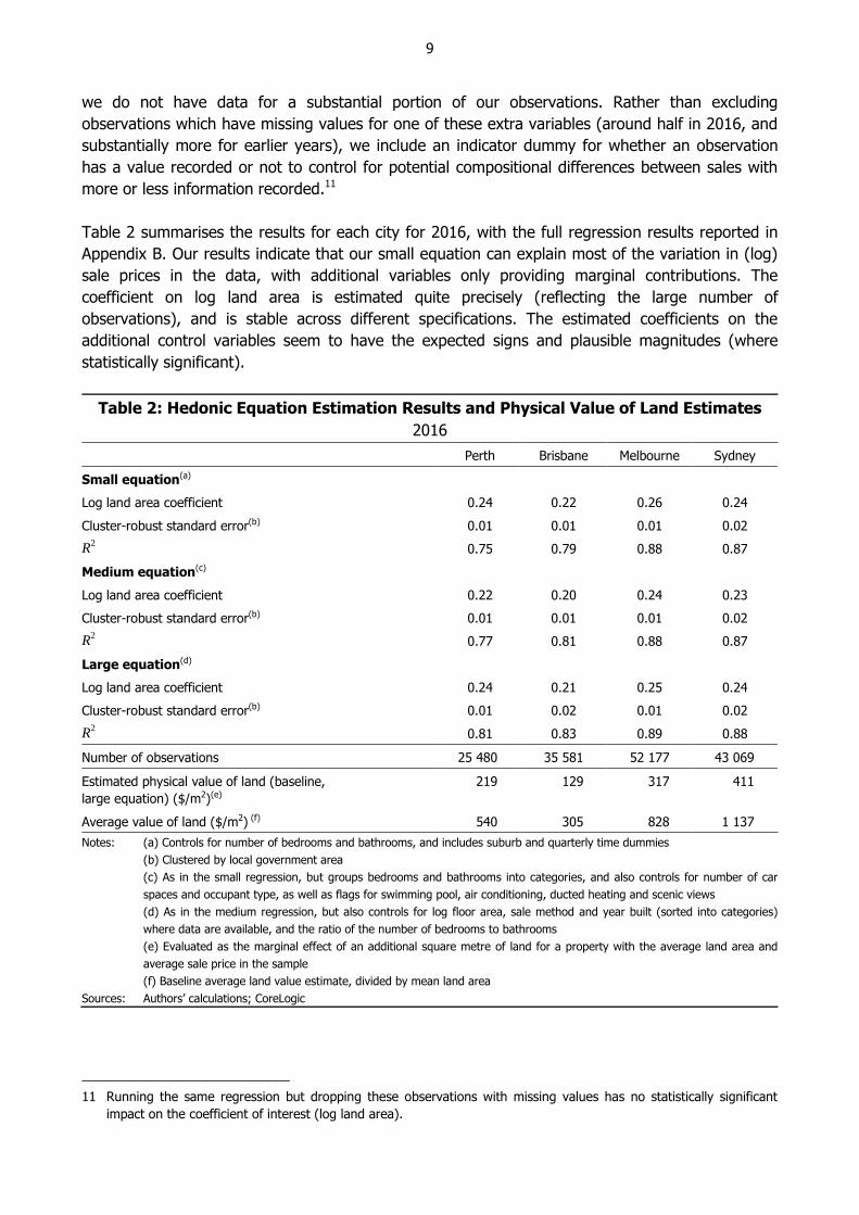
Table 2 summarises the results for each city for 2016, with the full regression results reported in

Appendix B. Our results indicate that our small equation can explain most of the variation in (log)

sale prices in the data, with additional variables only providing marginal contributions. The

coefficient on log land area is estimated quite precisely (reflecting the large number of

observations), and is stable across different specifications. The estimated coefficients on the

additional control variables seem to have the expected signs and plausible magnitudes (where

statistically significant).

Table 2: Hedonic Equation Estimation Results and Physical Value of Land Estimates

2016


Small equation(a)

Log land area coefficient 0.24 0.22 0.26 0.24

Cluster-robust standard error(b) 0.01 0.01 0.01 0.02

R2 0.75 0.79 0.88 0.87

Medium equation(c)



R2 0.77 0.81 0.88 0.87

Large equation(d)



R2 0.81 0.83 0.89 0.88

Number of observations 25 480 35 581 52 177 43 069

Estimated physical value of land (baseline,

large equation) ($/m2)(e)

219 129 317 411

Average value of land ($/m2) (f) 540 305 828 1 137

Notes: (a) Controls for number of bedrooms and bathrooms, and includes suburb and quarterly time dummies

(b) Clustered by local government area

(c) As in the small regression, but groups bedrooms and bathrooms into categories, and also controls for number of car

spaces and occupant type, as well as flags for swimming pool, air conditioning, ducted heating and scenic views

(d) As in the medium regression, but also controls for log floor area, sale method and year built (sorted into categories)

where data are available, and the ratio of the number of bedrooms to bathrooms

(e) Evaluated as the marginal effect of an additional square metre of land for a property with the average land area and

average sale price in the sample

(f) Baseline average land value estimate, divided by mean land area

Sources: Authors’ calculations; CoreLogic

11 Running the same regression but dropping these observations with missing values has no statistically significant

impact on the coefficient of interest (log land area).

10

To interpret our results, consider the estimated coefficient on log land area in our large equation

for Sydney of 0.24. This means that, holding other characteristics constant, house prices in a given

suburb would be bid up by approximately 0.24 per cent for every 1 per cent increase in land area.

For the average Sydney property, with a land area of 673 square metres and a value of

$1.16 million, that means an extra 6.73 square metres raises the property value by $2 764

(= $1 160 000 0.0024) or $411 a square metre.12 This contrasts with the average cost of land of

$1 137 per square metre. Equivalently, the marginal value to home owners of 673 square metres

of land is $276 000, but the block of land costs $765 000.13 Administrative scarcity means that

people have to pay the extra $489 000 above marginal cost for the right to have a structure on

that land. As shown in Table 2, similar calculations imply that in Brisbane, Melbourne and Perth the

physical value of land is also much less than the average value of land, although the difference is

smaller than in Sydney.

5. Zoning Effect Estimates

We now use our estimates to show that zoning restrictions are a major contributor to the cost of

housing, and the largest proximate cause of cross-city differences in average house prices.

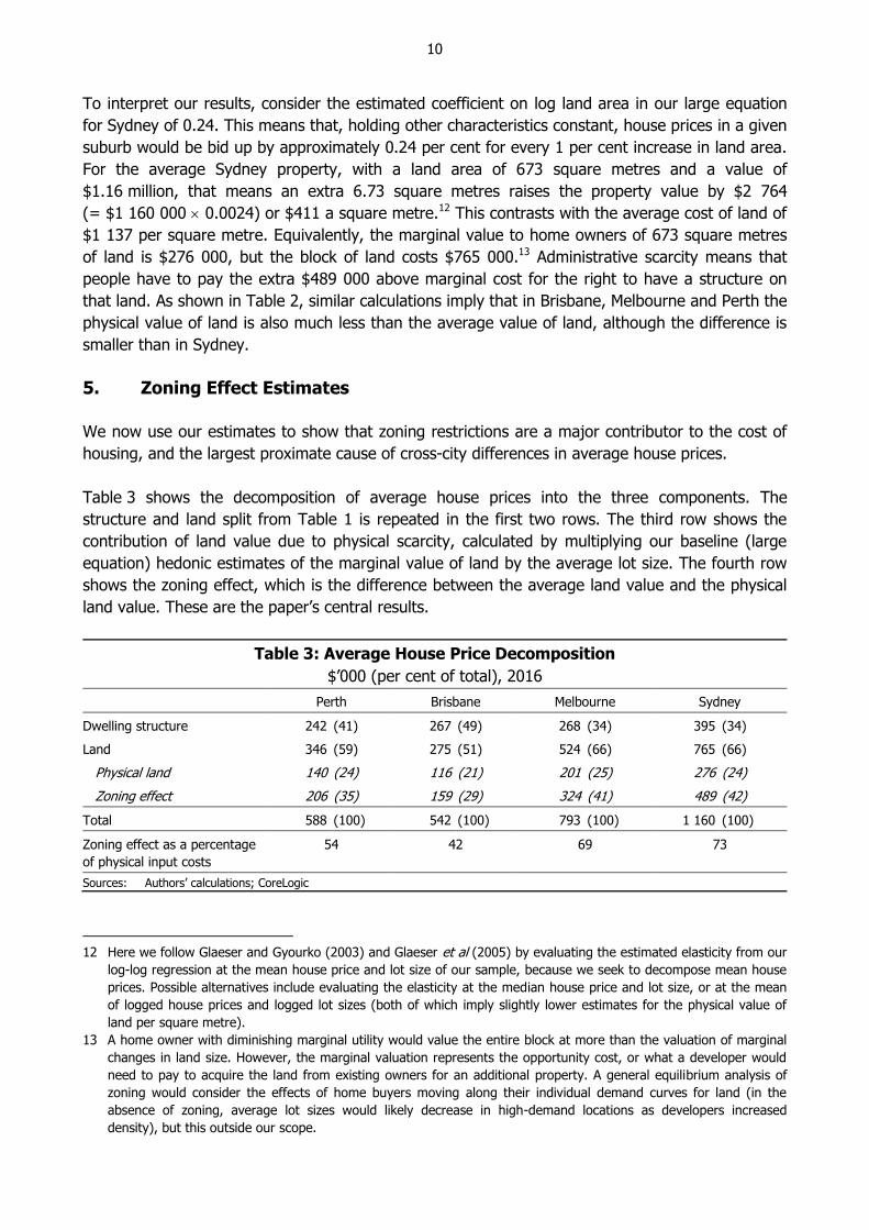
Table 3 shows the decomposition of average house prices into the three components. The

structure and land split from Table 1 is repeated in the first two rows. The third row shows the

contribution of land value due to physical scarcity, calculated by multiplying our baseline (large

equation) hedonic estimates of the marginal value of land by the average lot size. The fourth row

shows the zoning effect, which is the difference between the average land value and the physical

land value. These are the paper’s central results.

Table 3: Average House Price Decomposition

$’000 (per cent of total), 2016


Dwelling structure 242 (41) 267 (49) 268 (34) 395 (34)

Land 346 (59) 275 (51) 524 (66) 765 (66)

Physical land 140 (24) 116 (21) 201 (25) 276 (24)

Zoning effect 206 (35) 159 (29) 324 (41) 489 (42)

Total 588 (100) 542 (100) 793 (100) 1 160 (100)

Zoning effect as a percentage

of physical input costs

54 42 69 73


12 Here we follow Glaeser and Gyourko (2003) and Glaeser et al (2005) by evaluating the estimated elasticity from our

log-log regression at the mean house price and lot size of our sample, because we seek to decompose mean house

prices. Possible alternatives include evaluating the elasticity at the median house price and lot size, or at the mean

of logged house prices and logged lot sizes (both of which imply slightly lower estimates for the physical value of

land per square metre).

13 A home owner with diminishing marginal utility would value the entire block at more than the valuation of marginal

changes in land size. However, the marginal valuation represents the opportunity cost, or what a developer would

need to pay to acquire the land from existing owners for an additional property. A general equilibrium analysis of

zoning would consider the effects of home buyers moving along their individual demand curves for land (in the

absence of zoning, average lot sizes would likely decrease in high-demand locations as developers increased

density), but this outside our scope.

11

The zoning effect can be expressed as a percentage of the costs of the physical inputs or of the

total price. We alternate between the two, depending on the context. We estimate that zoning

restrictions raise the price of the average house in Sydney by 73 per cent above the value of the

physical inputs (structure and physical land) required to provide it. Corresponding effects are

69 per cent for Melbourne, 42 per cent for Brisbane and 54 per cent for Perth. As a share of total

property value, the contribution from zoning is 42 per cent in Sydney, 41 per cent in Melbourne,

29 per cent in Brisbane and 35 per cent in Perth. There are substantial differences between cities,

especially in dollar terms, with zoning restrictions adding only $159 000 to the cost of the average

house in Brisbane, compared with $489 000 in Sydney.

Estimates of the zoning effect in other countries span a wide range. The effect is estimated to be

large in cities with tight restrictions and negligible where building is unrestricted. Our estimates are

similar to estimated effects in cities with tight restrictions. For example, Glaeser et al (2005)

estimate zoning effects, as a share of total price, for 1998–99 of 53 per cent in San Francisco,

47 per cent in San Jose and 34 per cent in Los Angeles. Cheung et al (2009) estimate zoning

effects for 2005 of around 40 per cent for Miami and Orlando, 30 per cent for Tampa and 25 per

cent for Jacksonville. Lees (2018) estimates effects of 56 per cent in Auckland, 48 per cent in

Wellington and 32 per cent in Christchurch.

In important ways, our estimates are based on better data than was available to these earlier

studies. Where other estimates often rely on small samples, our regressions have sample sizes in

the tens of thousands. Where some other studies use self-assessed property values to estimate

the hedonic value of land, we use actual sale prices. Where other studies only have industry

construction cost estimates, we are able to use valuer general and ABS estimates also.

In contrast to the effect of zoning restrictions, differences in dwelling structure values across cities

account for relatively little of the variation in average sale prices. Our estimates of average

structure value for Australia are broadly similar (at 2017 exchange rates) to estimates for

New Zealand in Lees (2018), but almost 50 per cent higher than estimates for the United States

from Glaeser and Gyourko (2018) (see the Online Appendix, Section 1).

We estimate that the value of physical land for the average house in Sydney is higher than for

Melbourne, and substantially higher than for Brisbane or Perth. However, as a share of average

house prices these estimates are similar (between 21 and 25 per cent), and high compared with

overseas estimates. Physical land accounted for between 4 and 9 per cent of average house value

in Auckland, Wellington and Christchurch based on the numbers reported in Lees (2018).

Estimates in Glaeser and Gyourko (2003) imply that physical land accounted for between 3 and

12 per cent of total land value in the six cities with the highest average house prices in their study.

The relatively high physical land value that we find for Australian cities may reflect geographical

constraints facing the expansion of these cities (e.g. coasts and national parks), combined with

high demand reflecting population growth and low real interest rates.

In decomposing property values into the structure, physical land and zoning, some readers have

asked whether ‘location’ – as, for example, measured by our suburb dummies – should also be

allowed for, given that this is an attribute that buyers pay highly for. To the extent that land at a

location is physically scarce, the value of location will already be captured in our physical land

12

term. To the extent that land at a location is scarce because of administrative restrictions, it shows

up in the zoning effect.

5.1 Robustness of Our Hedonic Estimates

A central feature of our results is that the marginal value of land is less than the average value.

Our method for estimating the contribution of zoning restrictions to house prices is based on this

difference between marginal and average value, so sensitivity of our marginal land value estimates

to the functional form of our hedonic regression would be a concern.

Our baseline logarithmic specification is simple, but fits our data well. It is fairly common in the

literature, being used by previous hedonic house price applications, in both Australia

(e.g. Hansen 2006; CoreLogic 2017) and overseas (e.g. Glaeser et al 2005). Our estimates of the

log land area coefficient are not sensitive to the inclusion of control variables (as shown in Table 2

above) and are stable across time.

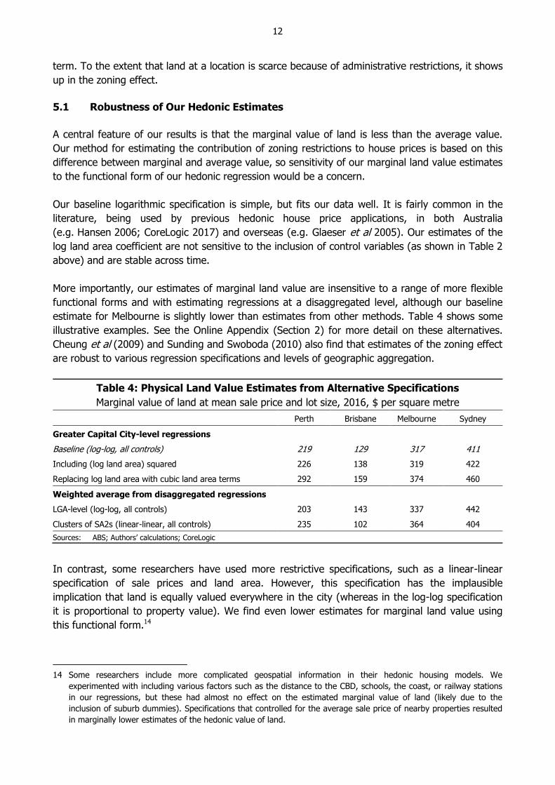
More importantly, our estimates of marginal land value are insensitive to a range of more flexible

functional forms and with estimating regressions at a disaggregated level, although our baseline

estimate for Melbourne is slightly lower than estimates from other methods. Table 4 shows some

illustrative examples. See the Online Appendix (Section 2) for more detail on these alternatives.

Cheung et al (2009) and Sunding and Swoboda (2010) also find that estimates of the zoning effect

are robust to various regression specifications and levels of geographic aggregation.

Table 4: Physical Land Value Estimates from Alternative Specifications

Marginal value of land at mean sale price and lot size, 2016, $ per square metre


Greater Capital City-level regressions

Baseline (log-log, all controls) 219 129 317 411

Including (log land area) squared 226 138 319 422

Replacing log land area with cubic land area terms 292 159 374 460

Weighted average from disaggregated regressions

LGA-level (log-log, all controls) 203 143 337 442

Clusters of SA2s (linear-linear, all controls) 235 102 364 404

Sources: ABS; Authors’ calculations; CoreLogic

In contrast, some researchers have used more restrictive specifications, such as a linear-linear

specification of sale prices and land area. However, this specification has the implausible

implication that land is equally valued everywhere in the city (whereas in the log-log specification

it is proportional to property value). We find even lower estimates for marginal land value using

this functional form.14

14 Some researchers include more complicated geospatial information in their hedonic housing models. We

experimented with including various factors such as the distance to the CBD, schools, the coast, or railway stations

in our regressions, but these had almost no effect on the estimated marginal value of land (likely due to the

inclusion of suburb dummies). Specifications that controlled for the average sale price of nearby properties resulted

in marginally lower estimates of the hedonic value of land.

13

Our hedonic estimates of the marginal value of land are similar to other hedonic housing studies of

Australian cities.

Hansen (2006, p 16) reports regressions of log house prices using Australian Property Monitors

data. His coefficient estimates on log land area are similar to ours for Sydney (0.28) and

Melbourne (0.19). However, he reports a much larger coefficient of 0.39 for Brisbane. One cause

of this difference could be that Hansen’s regressions are run on only a sub-sample of 1 per cent of

Brisbane sales due to missing values for a range of characteristics. In addition, Hansen’s sample

includes townhouses as well as detached houses, and controls for property zoning.

Syed, Hill and Melser (2008) construct hedonic house price indices for different regions of Sydney

from 2001 to 2006 using regressions of logged sale prices on a range of characteristics including

quadratic terms for lot size, and lot size interacted with a number of other variables. Their

estimated quadratic lot size coefficients for 2006 (p 57) imply that a 1 per cent increase in lot size

(for a property with a lot size of 635 square metres – the mean in our sample of sales in 2006)

would increase sale prices by 0.21 per cent, similar to our estimate of 0.24.

Frino et al (2010) report regressions of log house prices in Australian cities for the period 2005 to

2009. They report coefficients on log land area that are substantially lower than our findings:

0.10 for Sydney, 0.08 for Melbourne, 0.13 for Brisbane, and 0.16 for Perth. This appears to be

because they control for location at a much less granular level than we do (our coefficient

estimates are similar if we include dummies for the ABS Statistical Area Level 4 of each property

instead of the suburb).

5.2 Sensitivity of Our Zoning Effect Estimates to Inputs

Our zoning effect estimates are calculated indirectly, and so depend on our estimates of the other

components of the cost of housing. We now consider how sensitive our zoning effect estimates are

to changes in our estimates of structure value and physical land value. Overall, our baseline

estimates are reasonably robust.

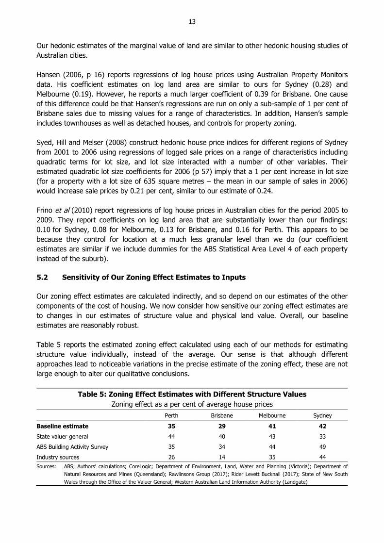
Table 5 reports the estimated zoning effect calculated using each of our methods for estimating

structure value individually, instead of the average. Our sense is that although different

approaches lead to noticeable variations in the precise estimate of the zoning effect, these are not

large enough to alter our qualitative conclusions.

Table 5: Zoning Effect Estimates with Different Structure Values

Zoning effect as a per cent of average house prices


Baseline estimate 35 29 41 42

State valuer general 44 40 43 33

ABS Building Activity Survey 35 34 44 49

Industry sources 26 14 35 44

Sources: ABS; Authors’ calculations; CoreLogic; Department of Environment, Land, Water and Planning (Victoria); Department of

Natural Resources and Mines (Queensland); Rawlinsons Group (2017); Rider Levett Bucknall (2017); State of New South

Wales through the Office of the Valuer General; Western Australian Land Information Authority (Landgate)

14

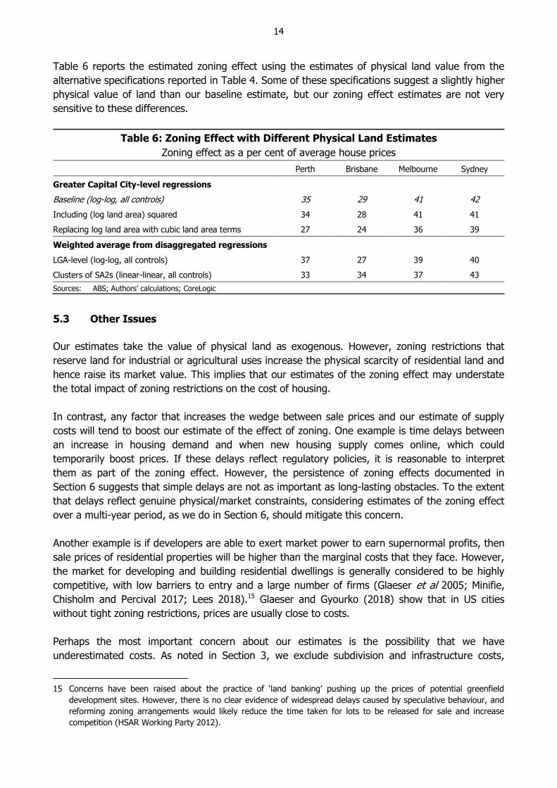
Table 6 reports the estimated zoning effect using the estimates of physical land value from the

alternative specifications reported in Table 4. Some of these specifications suggest a slightly higher

physical value of land than our baseline estimate, but our zoning effect estimates are not very

sensitive to these differences.

Table 6: Zoning Effect with Different Physical Land Estimates

Zoning effect as a per cent of average house prices


Greater Capital City-level regressions

Baseline (log-log, all controls) 35 29 41 42

Including (log land area) squared 34 28 41 41

Replacing log land area with cubic land area terms 27 24 36 39

Weighted average from disaggregated regressions

LGA-level (log-log, all controls) 37 27 39 40

Clusters of SA2s (linear-linear, all controls) 33 34 37 43


5.3 Other Issues

Our estimates take the value of physical land as exogenous. However, zoning restrictions that

reserve land for industrial or agricultural uses increase the physical scarcity of residential land and

hence raise its market value. This implies that our estimates of the zoning effect may understate

the total impact of zoning restrictions on the cost of housing.

In contrast, any factor that increases the wedge between sale prices and our estimate of supply

costs will tend to boost our estimate of the effect of zoning. One example is time delays between

an increase in housing demand and when new housing supply comes online, which could

temporarily boost prices. If these delays reflect regulatory policies, it is reasonable to interpret

them as part of the zoning effect. However, the persistence of zoning effects documented in

Section 6 suggests that simple delays are not as important as long-lasting obstacles. To the extent

that delays reflect genuine physical/market constraints, considering estimates of the zoning effect

over a multi-year period, as we do in Section 6, should mitigate this concern.

Another example is if developers are able to exert market power to earn supernormal profits, then

sale prices of residential properties will be higher than the marginal costs that they face. However,

the market for developing and building residential dwellings is generally considered to be highly

competitive, with low barriers to entry and a large number of firms (Glaeser et al 2005; Minifie,

Chisholm and Percival 2017; Lees 2018).15 Glaeser and Gyourko (2018) show that in US cities

without tight zoning restrictions, prices are usually close to costs.

Perhaps the most important concern about our estimates is the possibility that we have

underestimated costs. As noted in Section 3, we exclude subdivision and infrastructure costs,

15 Concerns have been raised about the practice of ‘land banking’ pushing up the prices of potential greenfield

development sites. However, there is no clear evidence of widespread delays caused by speculative behaviour, and

reforming zoning arrangements would likely reduce the time taken for lots to be released for sale and increase

competition (HSAR Working Party 2012).

15

which are substantial for greenfield developments but not for increasing housing density. We also

exclude adjustment costs, specifically when demolition of old structures is necessary for a change

in land use. When demolition is necessary, the cost of supply is not only the cost of land and new

structures, but also includes the acquisition cost of partially-depreciated structures.

We have excluded adjustment costs for two reasons. First, they are highly variable and difficult to

quantify. Second, house prices are determined on the margin, and marginal adjustment costs are

often low. Australia’s cities have low average density and heterogeneous housing stocks.16 So

underdeveloped blocks of land and heavily depreciated structures, for which adjustment costs are

low, are widespread. Substantial increases in density – for example, from large-lot detached

dwellings to high-rise apartments – reduce adjustment costs by spreading them across many new

dwellings. Moreover, increasing the density of new developments does not incur a marginal

adjustment cost. Adjustment costs are more likely to be material in already developed areas, and it

is possible that this (along with the cost of consolidating land parcels for high-rise development)

may further contribute to higher property values in inner-city areas, relative to the city fringe.

6. Decomposing Average House Prices over Time

Figure 2 shows a decomposition of property prices back to 1999. To extend our estimates of

structure value back in time, we adjust the estimates from Table 1 by movements in the producer

price index (PPI) – output of house construction series for each city’s corresponding state, and by

movements in the average floor area of houses sold in each city.17 To estimate the value of

physical land over time, we estimate separate regressions for each year back to 1999.

Given that housing supply takes time to respond to developments in demand (even in the absence

of zoning restrictions), looking at the zoning effect over a period of a few years may reduce

concerns that a gap between prices and costs reflects temporary supply shortages or delays.18

In all four cities, our estimate of the zoning effect increased rapidly as a share of average house

value over the early 2000s, alongside rapidly rising house prices. Subsequent to this initial rise, the

patterns across cities diverged somewhat. The increase in our zoning effect estimates over this

time period are likely due to existing zoning restrictions becoming more binding as demand has

risen, rather than a meaningful change in the restrictions themselves.

Our estimates suggest that while structure values have increased in all four cities since the early

2000s, they have declined substantially as a share of average house prices. Estimated physical

land values have increased more rapidly over time in Melbourne and Sydney than in Brisbane and

Perth, but have accounted for a relatively small share of the divergence in average house prices

between the four cities over the period.

16 As noted by Ellis (2013), Australian cities are less dense than the cities of any other sizeable country.

17 Changes in these state PPI series are almost identical to changes in the corresponding capital city CPI new dwelling

series, but for technical and conceptual reasons are slightly more appropriate for our use here. We also adjust for

the introduction of GST.

18 Although if the housing market (as an asset market) is forward looking, then expectations of a supply response

should offset this to a large degree.

16

Figure 2: House Price Decomposition

By city, mean


Our data extend earlier in time than shown in Figure 2. However, the contribution of land becomes

so small that property values fall within the range of our estimates of construction costs in

Brisbane and Melbourne. Estimates for early years would be decomposing measurement error.

Indeed, our earliest estimates of the zoning effect in Brisbane and Melbourne are slightly negative.

We suspect this arises because the industry-based approach to estimating structure value is too

high for these cities. Notwithstanding this, our decomposition suggests that zoning restrictions

were not a material constraint on housing development in these cities at this time – unlike in

Sydney, where the zoning effect is estimated to have been around 20 per cent of average sale

prices, even in 2000. This also shows that our methodology does not result in substantial

estimates of the zoning effect in every place and at every point in time.

7. Geographic Distribution of Zoning Effects within Cities

Figures 3–6 show estimates of the zoning effect for the average property in local government

areas (LGAs). We split property prices into structure values and land values in each LGA, using the

CoreLogic data on property prices and the valuer general estimates for land values for each LGA

(as this allows structure value to vary across LGAs for reasons other than just floor area).19 We

then estimate physical land values by running separate hedonic regressions for each LGA of the

form of our large regression in Section 4.20 Our estimate of the zoning effect by LGA is then the

remaining portion of land value not accounted for by the physical value.

19 As shown in Table 5, valuer general structure estimates imply a higher zoning effect estimate for Brisbane and Perth

and lower for Sydney than would an average of the three valuation approaches.

20 One difference is that we include sales from both 2015 and 2016 to estimate our hedonic equation, as the sample

size for some LGAs was very small using a single year, making estimation of the coefficients difficult. However, we

apply the estimated log land area coefficient only to the average sale price and land area of houses sold in 2016.

SydneySydney

20102004

250

500

750

1 000

$’000

250

500

750

1 000

$’000

Sale price

MelbourneMelbourne

20102004 2016

250

500

750

1 000

$’000

250

500

750

1 000

$’000

Zoning effect

BrisbaneBrisbane

2011200620010

250

500

750

1 000

$’000

0

250

500

750

1 000

$’000

Structure

PerthPerth

201120062001 20160

250

500

750

1 000

$’000

0

250

500

750

1 000

$’000

Physical land

17

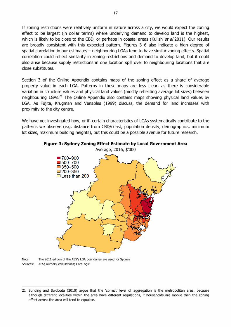
If zoning restrictions were relatively uniform in nature across a city, we would expect the zoning

effect to be largest (in dollar terms) where underlying demand to develop land is the highest,

which is likely to be close to the CBD, or perhaps in coastal areas (Kulish et al 2011). Our results

are broadly consistent with this expected pattern. Figures 3–6 also indicate a high degree of

spatial correlation in our estimates – neighbouring LGAs tend to have similar zoning effects. Spatial

correlation could reflect similarity in zoning restrictions and demand to develop land, but it could

also arise because supply restrictions in one location spill over to neighbouring locations that are

close substitutes.

Section 3 of the Online Appendix contains maps of the zoning effect as a share of average

property value in each LGA. Patterns in these maps are less clear, as there is considerable

variation in structure values and physical land values (mostly reflecting average lot sizes) between

neighbouring LGAs.21 The Online Appendix also contains maps showing physical land values by

LGA. As Fujita, Krugman and Venables (1999) discuss, the demand for land increases with

proximity to the city centre.

We have not investigated how, or if, certain characteristics of LGAs systematically contribute to the

patterns we observe (e.g. distance from CBD/coast, population density, demographics, minimum

lot sizes, maximum building heights), but this could be a possible avenue for future research.

Figure 3: Sydney Zoning Effect Estimate by Local Government Area

Average, 2016, $’000

Note: The 2011 edition of the ABS’s LGA boundaries are used for Sydney


21 Sunding and Swoboda (2010) argue that the ‘correct’ level of aggregation is the metropolitan area, because

although different localities within the area have different regulations, if households are mobile then the zoning

effect across the area will tend to equalise.

18

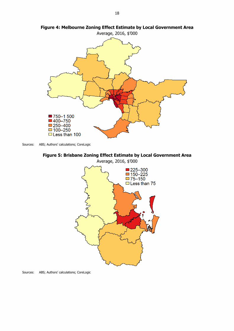
Figure 4: Melbourne Zoning Effect Estimate by Local Government Area

Average, 2016, $’000


Figure 5: Brisbane Zoning Effect Estimate by Local Government Area

Average, 2016, $’000


19

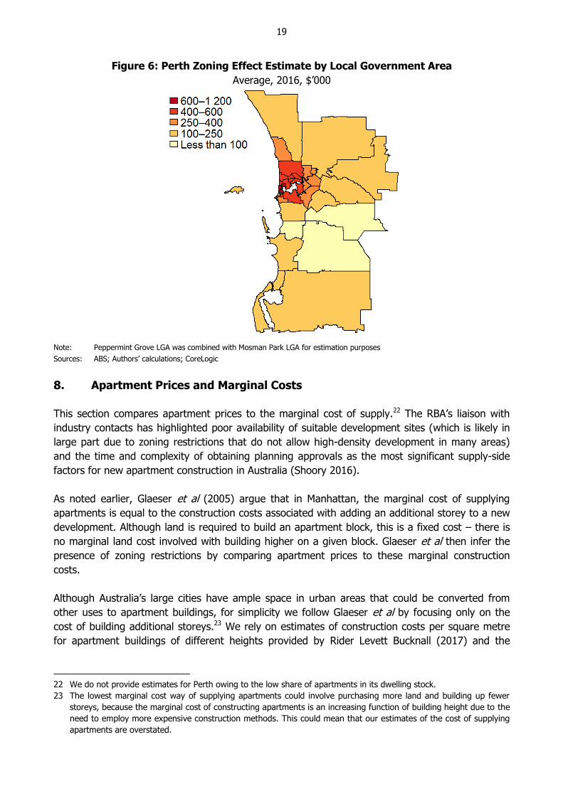
Figure 6: Perth Zoning Effect Estimate by Local Government Area

Average, 2016, $’000

Note: Peppermint Grove LGA was combined with Mosman Park LGA for estimation purposes


8. Apartment Prices and Marginal Costs

This section compares apartment prices to the marginal cost of supply.22 The RBA’s liaison with

industry contacts has highlighted poor availability of suitable development sites (which is likely in

large part due to zoning restrictions that do not allow high-density development in many areas)

and the time and complexity of obtaining planning approvals as the most significant supply-side

factors for new apartment construction in Australia (Shoory 2016).

As noted earlier, Glaeser et al (2005) argue that in Manhattan, the marginal cost of supplying

apartments is equal to the construction costs associated with adding an additional storey to a new

development. Although land is required to build an apartment block, this is a fixed cost – there is

no marginal land cost involved with building higher on a given block. Glaeser et al then infer the

presence of zoning restrictions by comparing apartment prices to these marginal construction

costs.

Although Australia’s large cities have ample space in urban areas that could be converted from

other uses to apartment buildings, for simplicity we follow Glaeser et al by focusing only on the

cost of building additional storeys.23 We rely on estimates of construction costs per square metre

for apartment buildings of different heights provided by Rider Levett Bucknall (2017) and the

22 We do not provide estimates for Perth owing to the low share of apartments in its dwelling stock.

23 The lowest marginal cost way of supplying apartments could involve purchasing more land and building up fewer

storeys, because the marginal cost of constructing apartments is an increasing function of building height due to the

need to employ more expensive construction methods. This could mean that our estimates of the cost of supplying

apartments are overstated.

20

CoreLogic unit record dataset to calculate average sale prices. A detailed discussion of our data

and methodology is in the Online Appendix (Section 4).

For this exercise, we consider the marginal cost of constructing a 20-storey apartment building

relative to a 10-storey building. RBA liaison evidence and Daley et al (2018, p 50) indicate that

buildings in this range are representative of a large share of the apartment market in major cities.

We make an allowance for other marginal costs associated with increasing the size of an

apartment project, such as providing common areas, professional fees and an entrepreneurial

return. Finally, we adjust costs for earlier time periods using the corresponding state PPI – output

of other residential building construction series, and scale to the average size of apartments sold in

each city during the corresponding period (e.g. 79 square metres in Sydney in 2016).

Our analysis of the Rider Levett Bucknall estimates suggests that, on average, it would cost about

$470 000 to add an extra apartment to a 10–20 storey building in Sydney in 2016. This is the

marginal cost; the average variable cost is $435 000. Although comparison can be difficult,

alternative data sources point to similar, or somewhat smaller, estimates. For example, estimates

by the CIE (2011) suggest a typical 100 square metre Sydney apartment costs $438 000 to build

(adjusted to 2016 dollars using the appropriate PPI), whereas our estimates imply that such an

apartment would cost $552 000 (average cost in a 10–20 storey building). Discussions with

industry participants tend to suggest average construction costs cluster around $300 000 to

$500 000, with more dispersion in estimates of fees, margins and overheads.

Our analysis of the CoreLogic dataset indicates that the average Sydney apartment sold for

$870 000 in 2016.24 This is about $400 000 (85 per cent) more than our estimate of marginal cost,

representing 46 per cent of the sale price. As with detached houses, this $400 000 wedge

represents an arbitrage opportunity. The reason that builders do not exploit it is that they are

prohibited from doing so by zoning regulations.25 See Moore (2012) for an example. Similar

analysis, summarised in Table 7, implies that zoning restrictions added $120 000 to the cost of

apartments in Melbourne and $110 000 in Brisbane. Our estimate of the zoning contribution for

Sydney is broadly in line with the findings of Glaeser et al (2005), who found that zoning

accounted for around half of the cost of apartments in Manhattan in 2002, but smaller than

Lees (2018), who found that zoning accounted for around 70 per cent of the cost of apartments in

Auckland.

24 New apartments sold for somewhat more. Because we are using construction costs, we are likely to be overstating

replacement value for apartments due to depreciation (renovations are less likely to provide a positive offset than in

the case of detached dwellings).

25 To the extent that planning regulations increase construction costs (rather than creating a wedge between costs and

prices), for instance through prescriptive building design and materials requirements, then this effect of regulation

on prices will not be captured in our estimates.

21

Table 7: Apartment Cost and Prices

2016

Brisbane Melbourne Sydney

Marginal cost, per square metre of floor area ($/m2) 4 953 5 731 5 985

Average floor area of apartments sold (m2) 87 68 79

Marginal cost, per apartment ($’000) 429 390 471

Average apartment sale price ($’000) 539 510 870

Zoning effect ($’000) 110 120 399

Zoning effect (% of marginal cost) 26 30 85

Sources: ABS; Authors’ calculations; CoreLogic; Rider Levett Bucknall (2017)

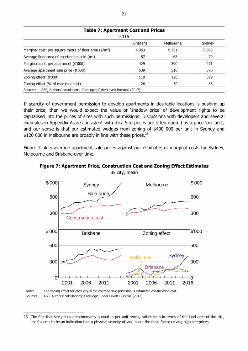
If scarcity of government permission to develop apartments in desirable locations is pushing up

their price, then we would expect the value or ‘shadow price’ of development rights to be

capitalised into the prices of sites with such permissions. Discussions with developers and several

examples in Appendix A are consistent with this. Site prices are often quoted as a price ‘per unit’,

and our sense is that our estimated wedges from zoning of $400 000 per unit in Sydney and

$120 000 in Melbourne are broadly in line with these prices.26

Figure 7 plots average apartment sale prices against our estimates of marginal costs for Sydney,

Melbourne and Brisbane over time.

Figure 7: Apartment Price, Construction Cost and Zoning Effect Estimates

By city, mean

Note: The zoning effect for each city is the average sale price minus estimated construction cost

Sources: ABS; Authors’ calculations; CoreLogic; Rider Levett Bucknall (2017)

26 The fact that site prices are commonly quoted in per unit terms, rather than in terms of the land area of the site,

itself seems to be an indication that a physical scarcity of land is not the main factor driving high site prices.

Sydney

300

600

$’000

Sale price

Construction cost

Melbourne

300

600

$’000

Brisbane

2011200620010

300

600

$’000 Zoning effect

201120062001 20160

300

600

$’000

SydneyMelbourne

Brisbane

22

Over the period from 1999 to 2006, we estimate that the gap between sale prices and marginal

costs was low and broadly stable in all three cities, although the gap was slightly larger on average

in Sydney ($121 000 versus $60 000 in Brisbane and $47 000 in Melbourne). This analysis

suggests that zoning was not an important constraint on apartment development in Brisbane or

Melbourne over this period.

In both Melbourne and Brisbane, marginal costs were broadly unchanged over the period from

2006 to 2016. However, average sale prices rose slightly, and so the gap between sale prices and

costs has been somewhat higher in recent years. In Sydney, costs rose slightly over the same

period, but apartment sales prices increased much more sharply. As a result, the gap between

prices and costs – the zoning effect – has increased substantially in Sydney over the past decade.

Our estimates of apartment costs involve several assumptions and are somewhat uncertain. They

are not comprehensive, but we believe they are representative of a large share of the apartment

market. Moreover, the RBA’s discussions with developers suggest that our overall numbers are in

line with widely used rules of thumb in the industry. The results do not seem to be sensitive to

moderate variations in the assumptions. More direct data would be useful. However, we would be

surprised if it were to indicate a very different contribution of zoning to apartment prices.

9. Discussion

Overall, our results suggest that development restrictions (interacting with increasing demand)

have contributed materially to the significant rise in housing prices in Australia’s largest cities since

the late 1990s, pushing prices substantially above the supply costs of their physical inputs.

Although we find that differences in the value of dwelling structures and the physical value of land

account for some of the variation in average housing prices across the four cities we examine, our

zoning effect estimates account for the majority of the differences. We also find evidence of a

large gap opening up between apartment sale prices and construction costs over recent years,

especially in Sydney. This suggests that zoning constraints are also important in the market for

high-density dwellings.

We estimate that zoning restrictions raise detached house prices by 73 per cent of marginal costs

in Sydney, for example. We emphasise that this is not the amount that house prices would fall in

the absence of zoning. As discussed in our introduction, that would require estimating supply and

demand responses, which is beyond our scope. We also note that physical land costs are higher in

Australian cities (particularly Sydney) than overseas. So even if zoning restrictions were relaxed,

housing in Australia would remain expensive relative to cities where zoning is permissive and land

is less physically scarce.

Ideally, policy with respect to zoning would reflect a weighing of the benefits and costs. Our

analysis contributes to such a decision by quantifying some important costs. These should be

offset against the benefits from zoning, such as offsetting the negative externalities of intensified

or uncoordinated development. Gyourko and Molloy (2015) discuss the evidence on these issues

and conclude that the overall efficiency losses from constraints on residential development may be

large, with costs outweighing benefits by a substantial margin. Subsequent research (Albouy and

Ehrlich 2017) supports this conclusion. However, both these studies note that the benefits of most

forms of zoning regulations are difficult to quantify.

23

As Furman (2015) discusses, zoning regulations have some important effects that go beyond those

we quantify. As they become more binding and contribute to increases in property prices, they

represent a wealth transfer from future home buyers to current home owners (see, for example,

the discussion in Lowe (2015)). They also result in higher rents as the supply of housing is

constricted. Both of these factors may increase inequality. La Cava (2016) and Glaeser and

Gyourko (2018) emphasise rising house values in supply constrained markets as a driver of

changes in the distribution of wealth and income in the United States. Murray and Frijters (2015)

argue that many of the benefits seem to accrue to those with political connections and can be

dissipated in rent-seeking.

Development restrictions also reduce the responsiveness of the housing stock to changes in

preferences and relative prices. This can ‘lock in’ an increasingly obsolete urban structure (Kelly,

Weidmann and Walsh 2011). Cheshire, Hilber and Koster (2018) find that planning restrictions lead

to a substantial misallocation of housing resources in England. Perhaps more importantly, these

restrictions prevent labour from being allocated to where it is most productive. Estimates for the

United States suggest these effects are large (Hseih and Moretti 2015; Glaeser and Gyourko 2018;

Herkenhoff, Ohanian and Prescott 2018). Zoning restrictions reduce the elasticity of housing

supply, making housing prices more responsive to changes in underlying demand. As Glaeser,

Gyourko and Saiz (2008) document, this means that house prices are more variable than

otherwise, with potentially negative consequences for financial and price stability.

If housing demand continues to grow, as seems likely, then existing zoning restrictions will bind

more tightly and place continuing upward pressure on housing prices. Policy changes that make

zoning restrictions less binding, whether directly (e.g. increasing building height limits) or

indirectly, via reducing underlying demand for land in areas where restrictions are binding

(e.g. improving transport infrastructure), could reduce this upward pressure on housing prices.

24

Appendix A: Examples of Zoning Effects on Land and Property Values

Some examples of reports of large effects from zoning changes, compiled from a few hours

googling:

Michael Coco, a real estate agent, estimates that properties on the south side of Derby St,

Penrith, zoned for two-storey developments, are worth $600 000 while those on the north side,

zoned for six storeys, are worth $1 million (Jones 2016). Some properties on the north side

reportedly doubled in value overnight when the rezoning was announced.

Kulish et al (2011, p 30) cite estimates that the inclusion of agricultural land with the urban

growth boundary of Melbourne raises its value from below $35 000 a hectare to above

$300 000 a hectare. They also describe (fn 23) how the relaxation of zoning restrictions on

property in St Leonards in Sydney raised the land value from $3 million to $14 million.

According to Moran (2005, p 26), ‘Soon after the [Melbourne’s] Urban Growth Boundary was

introduced, land brought inside it, say, around Whittlesea, was selling at some $600,000 per

hectare where previously before the Boundary de facto rezoned it as housing it cost $150,000–

200,000 per hectare’.

Inner West Council (2016, p 27) report that rezoning a 1 000 square metre block of land in

Sydney’s inner west from industrial to eight-storey apartments changes the land value from

$2 million to $10.7 million.

Murray and Frijters (2015) report that the rezoning of 13 000 hectares in south-east

Queensland from rural to residential between 2008 and 2010 raised land values by $700 million.

Wallace Zagoridis, a developer, estimates that the value of his $8 million site was halved when

Ku-ring-gai Council reduced the permitted height of his project from seven to five storeys

(Moore 2012).

Chong (2015) lists large profits being made on former industrial sites that have been rezoned

for residential development in Sydney. For example, the Goodman group made profits of

$400 million to $600 million; the Dexus Property group expected profits of $90 million. A

6.9 hectare site near Erskineville, purchased for $16 million was sold for $350 million after

rezoning. Two sites in Rosebery initially valued at $96 million were sold for $190 million.

Consolidating nine houses in St Leonards, valued at up to $18 million, in a site for

200 apartments, raised the land value to $55 million.

Land prices doubled in the Montague precinct of Fishermans Bend in Melbourne after the

industrial area was rezoned to allow for residential development without mandatory height

limits (Johanson 2012).

Zhou (2017) reports that sites in Melbourne with approved plans and permits for medium-

density development are selling for a significant premium, with approvals adding several

hundreds of thousands of dollars to property values.

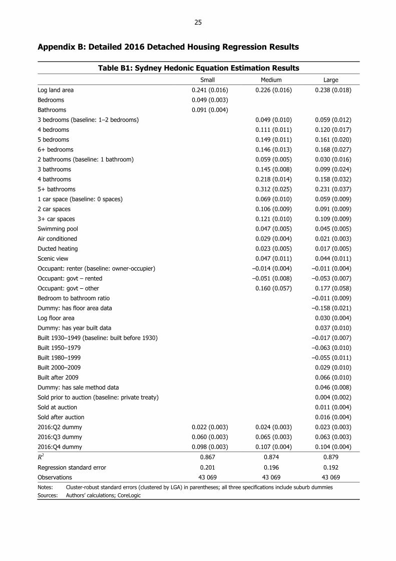
25

Appendix B: Detailed 2016 Detached Housing Regression Results

Table B1: Sydney Hedonic Equation Estimation Results

Small Medium Large

Log land area 0.241 (0.016) 0.226 (0.016) 0.238 (0.018)

Bedrooms 0.049 (0.003)

Bathrooms 0.091 (0.004)

3 bedrooms (baseline: 1–2 bedrooms) 0.049 (0.010) 0.059 (0.012)

4 bedrooms 0.111 (0.011) 0.120 (0.017)

5 bedrooms 0.149 (0.011) 0.161 (0.020)

6+ bedrooms 0.146 (0.013) 0.168 (0.027)

2 bathrooms (baseline: 1 bathroom) 0.059 (0.005) 0.030 (0.016)

3 bathrooms 0.145 (0.008) 0.099 (0.024)

4 bathrooms 0.218 (0.014) 0.158 (0.032)

5+ bathrooms 0.312 (0.025) 0.231 (0.037)

1 car space (baseline: 0 spaces) 0.069 (0.010) 0.059 (0.009)

2 car spaces 0.106 (0.009) 0.091 (0.009)

3+ car spaces 0.121 (0.010) 0.109 (0.009)

Swimming pool 0.047 (0.005) 0.045 (0.005)

Air conditioned 0.029 (0.004) 0.021 (0.003)

Ducted heating 0.023 (0.005) 0.017 (0.005)

Scenic view 0.047 (0.011) 0.044 (0.011)

Occupant: renter (baseline: owner-occupier) –0.014 (0.004) –0.011 (0.004)

Occupant: govt – rented –0.051 (0.008) –0.053 (0.007)

Occupant: govt – other 0.160 (0.057) 0.177 (0.058)

Bedroom to bathroom ratio –0.011 (0.009)

Dummy: has floor area data –0.158 (0.021)

Log floor area 0.030 (0.004)

Dummy: has year built data 0.037 (0.010)

Built 1930–1949 (baseline: built before 1930) –0.017 (0.007)

Built 1950–1979 –0.063 (0.010)

Built 1980–1999 –0.055 (0.011)

Built 2000–2009 0.029 (0.010)

Built after 2009 0.066 (0.010)

Dummy: has sale method data 0.046 (0.008)

Sold prior to auction (baseline: private treaty) 0.004 (0.002)

Sold at auction 0.011 (0.004)

Sold after auction 0.016 (0.004)

2016:Q2 dummy 0.022 (0.003) 0.024 (0.003) 0.023 (0.003)

2016:Q3 dummy 0.060 (0.003) 0.065 (0.003) 0.063 (0.003)

2016:Q4 dummy 0.098 (0.003) 0.107 (0.004) 0.104 (0.004)

R2 0.867 0.874 0.879

Regression standard error 0.201 0.196 0.192

Observations 43 069 43 069 43 069

Notes: Cluster-robust standard errors (clustered by LGA) in parentheses; all three specifications include suburb dummies


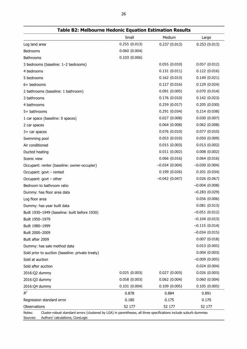
26

Table B2: Melbourne Hedonic Equation Estimation Results

Small Medium Large

Log land area 0.255 (0.013) 0.237 (0.013) 0.253 (0.013)

Bedrooms 0.060 (0.004)

Bathrooms 0.103 (0.006)


4 bedrooms 0.131 (0.011) 0.122 (0.016)

5 bedrooms 0.162 (0.013) 0.149 (0.021)

6+ bedrooms 0.127 (0.016) 0.129 (0.024)


3 bathrooms 0.176 (0.010) 0.142 (0.023)

4 bathrooms 0.259 (0.017) 0.205 (0.030)

5+ bathrooms 0.291 (0.034) 0.214 (0.038)

1 car space (baseline: 0 spaces) 0.027 (0.008) 0.030 (0.007)

2 car spaces 0.064 (0.008) 0.062 (0.008)

3+ car spaces 0.076 (0.010) 0.077 (0.010)

Swimming pool 0.053 (0.010) 0.050 (0.009)

Air conditioned 0.015 (0.003) 0.013 (0.002)

Ducted heating 0.011 (0.002) 0.008 (0.002)

Scenic view 0.066 (0.016) 0.064 (0.016)


Occupant: govt – rented 0.199 (0.026) 0.201 (0.034)

Occupant: govt – other –0.042 (0.047) 0.026 (0.067)






Built 1950–1979 –0.104 (0.013)

Built 1980–1999 –0.115 (0.014)

Built 2000–2009 –0.034 (0.015)

Built after 2009 0.007 (0.018)



Sold at auction –0.009 (0.005)


2016:Q2 dummy 0.025 (0.003) 0.027 (0.003) 0.026 (0.003)

2016:Q3 dummy 0.058 (0.003) 0.062 (0.004) 0.060 (0.004)

2016:Q4 dummy 0.101 (0.004) 0.109 (0.005) 0.105 (0.005)

R2 0.878 0.884 0.891


Observations 52 177 52 177 52 177



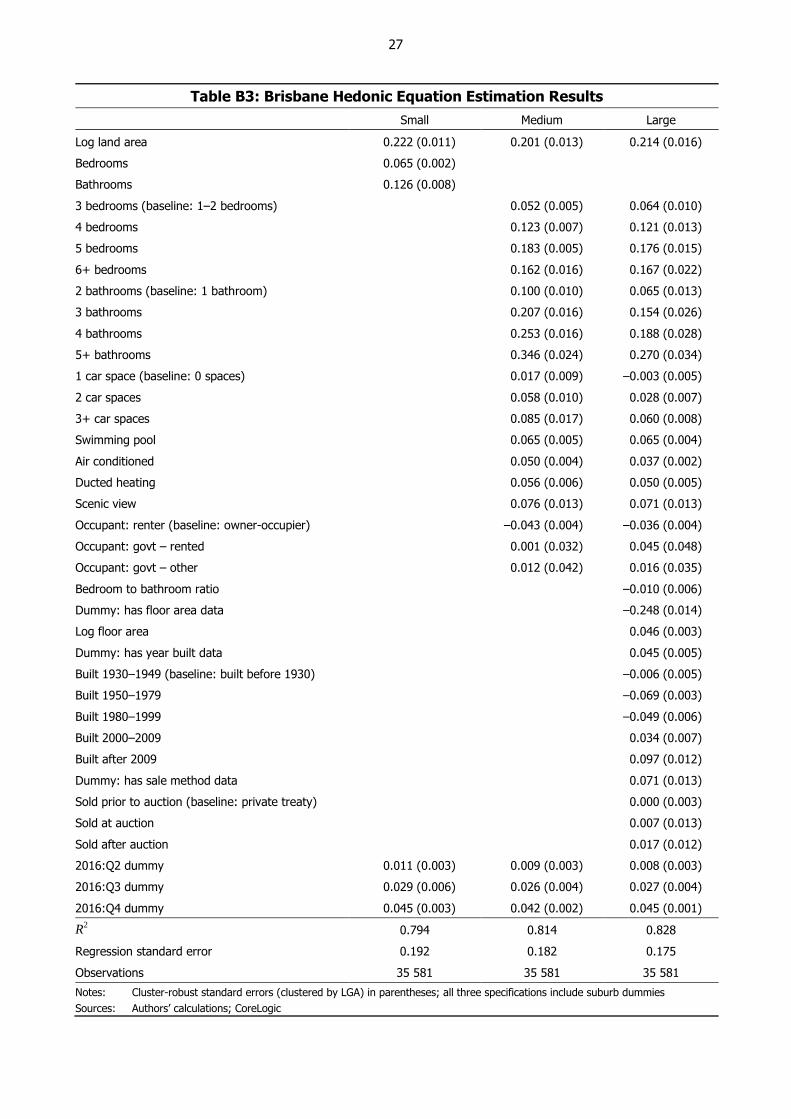
27

Table B3: Brisbane Hedonic Equation Estimation Results

Small Medium Large

Log land area 0.222 (0.011) 0.201 (0.013) 0.214 (0.016)

Bedrooms 0.065 (0.002)

Bathrooms 0.126 (0.008)


4 bedrooms 0.123 (0.007) 0.121 (0.013)

5 bedrooms 0.183 (0.005) 0.176 (0.015)

6+ bedrooms 0.162 (0.016) 0.167 (0.022)


3 bathrooms 0.207 (0.016) 0.154 (0.026)

4 bathrooms 0.253 (0.016) 0.188 (0.028)

5+ bathrooms 0.346 (0.024) 0.270 (0.034)

1 car space (baseline: 0 spaces) 0.017 (0.009) –0.003 (0.005)

2 car spaces 0.058 (0.010) 0.028 (0.007)

3+ car spaces 0.085 (0.017) 0.060 (0.008)

Swimming pool 0.065 (0.005) 0.065 (0.004)

Air conditioned 0.050 (0.004) 0.037 (0.002)

Ducted heating 0.056 (0.006) 0.050 (0.005)

Scenic view 0.076 (0.013) 0.071 (0.013)


Occupant: govt – rented 0.001 (0.032) 0.045 (0.048)

Occupant: govt – other 0.012 (0.042) 0.016 (0.035)






Built 1950–1979 –0.069 (0.003)

Built 1980–1999 –0.049 (0.006)

Built 2000–2009 0.034 (0.007)

Built after 2009 0.097 (0.012)





2016:Q2 dummy 0.011 (0.003) 0.009 (0.003) 0.008 (0.003)

2016:Q3 dummy 0.029 (0.006) 0.026 (0.004) 0.027 (0.004)

2016:Q4 dummy 0.045 (0.003) 0.042 (0.002) 0.045 (0.001)

R2 0.794 0.814 0.828


Observations 35 581 35 581 35 581



28

Table B4: Perth Hedonic Equation Estimation Results

Small Medium Large

Log land area 0.243 (0.008) 0.224 (0.009) 0.238 (0.010)

Bedrooms 0.061 (0.005)

Bathrooms 0.156 (0.009)


4 bedrooms 0.106 (0.014) 0.075 (0.028)

5 bedrooms 0.160 (0.013) 0.128 (0.034)

6+ bedrooms 0.081 (0.022) 0.072 (0.043)


3 bathrooms 0.273 (0.014) 0.168 (0.038)

4 bathrooms 0.316 (0.035) 0.200 (0.057)

5+ bathrooms 0.149 (0.113) 0.037 (0.110)

1 car space (baseline: 0 spaces) –0.025 (0.016) –0.046 (0.014)

2 car spaces 0.042 (0.017) –0.012 (0.015)

3+ car spaces 0.076 (0.018) 0.022 (0.015)

Swimming pool 0.064 (0.005) 0.065 (0.004)

Air conditioned 0.048 (0.008) 0.021 (0.005)

Ducted heating –0.005 (0.005) –0.001 (0.005)

Scenic view 0.110 (0.023) 0.101 (0.021)


Occupant: govt – rented –0.027 (0.022) 0.027 (0.024)

Occupant: govt – other –0.142 (0.028) –0.149 (0.031)






Built 1950–1979 –0.107 (0.022)

Built 1980–1999 –0.100 (0.022)

Built 2000–2009 0.015 (0.026)

Built after 2009 0.080 (0.026)





2016:Q2 dummy –0.012 (0.005) –0.011 (0.005) –0.015 (0.004)

2016:Q3 dummy –0.020 (0.005) –0.017 (0.005) –0.025 (0.005)

2016:Q4 dummy –0.028 (0.006) –0.019 (0.006) –0.027 (0.005)

R2 0.751 0.773 0.812


Observations 25 480 25 480 25 480



29

References

Albouy D and G Ehrlich (2017), ‘Housing Productivity and the Social Cost of Land-Use Restrictions’, NBER

Working Paper No 18110, rev December.

CEDA (Committee for Economic Development of Australia) (2017), Housing Australia, Research

report, Committee for Economic Development of Australia, Melbourne.

Cheshire PC and CAL Hilber (2008), ‘Office Space Supply Restrictions in Britain: The Political Economy of

Market Revenge’, The Economic Journal, 118(529), pp F185–F221.

Cheshire PC, CAL Hilber and HRA Koster (2018), ‘Empty Homes, Longer Commutes: The Unintended

Consequences of More Restrictive Local Planning’, Journal of Public Economics, 158, pp 126–151.

Cheung R, K Ihlanfeldt and T Mayock (2009), ‘The Regulatory Tax and House Price Appreciation in

Florida’, Journal of Housing Economics, 18(1), pp 34–48.

Chong F (2015), ‘The Property Players Cashing in on Sydney’s Rezoned Land’, The Australian online,

15 April, viewed January 2018. Available at <http://www.theaustralian.com.au/business/

business-spectator/the-property-players-cashing-in-on-sydneys-rezoned-land/news-story/

a76e65f878b8fd2fc17e55f1039b4174>.

CIE (Centre for International Economics) (2011), ‘Taxation of the Housing Sector’, Final report

prepared for the Housing Industry Association, September.

CIE (2013), ‘Reform of the NSW Planning System’, Final report prepared for NSW Planning and

Infrastructure, October.

CIE and ARUP (2012), ‘Costs and Benefits of Alternative Growth Scenarios for Sydney’, Final report

prepared for NSW Planning and Infrastructure, August.

CoreLogic (2017), ‘Residential Property Index Series’, August, viewed January 2018. Available at

<https://www.corelogic.com.au/sites/default/files/2017-09/CoreLogicHPISeriesMethodologyAug2017.pdf>.

Daley J, B Coates and T Wiltshire (2018), Housing Affordability: Re-imagining the Australian Dream,

Grattan Institute, Melbourne.

Ellis L (2013), ‘Housing and Mortgage Markets: The Long Run, the Short Run and the Uncertainty in

Between’, Address to the Citibank Property Conference, Sydney, 23 April.

Fox R and R Finlay (2012), ‘Dwelling Prices and Household Income’, RBA Bulletin, December, pp 13–22.

Frino A, A Lepone, V Mollica and A Vassallo (2010), ‘The Impact of Auctions on Residential Sale

Prices: Australian Evidence’, Australasian Accounting, Business and Finance Journal, 4(3), pp 3–22.

Fujita M, P Krugman and AJ Venables (1999), The Spatial Economy: Cities, Regions, and International

Trade, The MIT Press, Cambridge.

30

Furman J (2015), ‘Barriers to Shared Growth: The Case of Land Use Regulation and Economic Rents’,

Keynote address given at ‘Data, Demand and Demographics: A Symposium on Housing Finance’, Co-hosted

by the Urban Institute and CoreLogic, Washington DC, 20 November.

Glaeser EL and J Gyourko (2003), ‘The Impact of Building Restrictions on Housing Affordability’,

Economic Policy Review, 9(2), pp 21–39.

Glaeser EL and J Gyourko (2018), ‘The Economic Implications of Housing Supply’, Journal of Economic

Perspectives, 32(1), pp 3–30.

Glaeser EL, J Gyourko and A Saiz (2008), ‘Housing Supply and Housing Bubbles’, Journal of Urban

Economics, 64(2), pp 198–217.

Glaeser EL, J Gyourko and R Saks (2005), ‘Why is Manhattan So Expensive? Regulation and the Rise in

Housing Prices’, The Journal of Law & Economics, 48(2), pp 331–369.

Gyourko J and R Molloy (2015), ‘Regulation and Housing Supply’, in G Duranton, JV Henderson and

W Strange (eds), Handbook of Regional and Urban Economics: Volume 5B, Handbooks in Economics, North-

Holland, Amsterdam, pp 1289–1337.

Hansen J (2006), ‘Australian House Prices: A Comparison of Hedonic and Repeat-Sales Measures’, RBA

Research Discussion Paper No 2006-03.

Herkenhoff KF, LE Ohanian and EC Prescott (2018), ‘Tarnishing the Golden and Empire States: Land-

Use Restrictions and the U.S. Economic Slowdown’, Journal of Monetary Economics, 93, pp 89–109.

Hilber CAL and W Vermeulen (2016), ‘The Impact of Supply Constraints on House Prices in England’,

The Economic Journal, 126(591), pp 358–405.

Hill RJ and M Scholz (2014), ‘Incorporating Geospatial Data in House Price Indexes: A Hedonic

Imputation Approach with Splines’, University of Graz, Graz Economics Papers 2014-05.

Hodges J (2015), ‘Questions on Notice following Australian Bureau of Statistics’ Submission to the House

of Representatives Home Ownership Inquiry’, 5.2 Supplementary to Submission 5, Submission to the House

of Representatives Standing Committee on Economics Inquiry into Home Ownership, 24 July. Available at

<https://www.aph.gov.au/DocumentStore.ashx?id=652af284-b3ee-4840-9833-de62a89bdf8d&subId

=353206>.

Housing Industry Association (2011), ‘The Taxation Burden on the Australian New Housing Sector’,

Summary. Available at <https://hia.com.au/-/media/HIA-Website/Files/Media-Centre/Submissions/2011/Tax-

Forum-Submission-Background.ashx?la=en&hash=A0A2DFB9CB843F967A696F4DFB81238C01FC07AC>.

HSAR (Housing Supply and Affordability Reform) Working Party (2012), ‘Housing Supply and

Affordability Reform’, Report to the Council of Australian Governments, September.

Hseih C-T and E Moretti (2015), ‘Housing Constraints and Spatial Misallocation’, NBER Working Paper

No 21154, rev May 2017.

Hsieh W, D Norman and D Orsmond (2012), ‘Supply-Side Issues in the Housing Sector’, RBA Bulletin,

September, pp 11–19.

31

Inner West Council (2016), ‘Position Paper: Best Practice in Value Capture’, rev March 2017. Available at

<https://www.innerwest.nsw.gov.au/ArticleDocuments/296/Best%20Practice%20in%20Value%

20Capture.pdf.aspx>.

Johanson S (2012), ‘Developers in the Zone on New Industrial Landscape’, The Sydney Morning Herald

online, 5 December, viewed January 2018. Available at <http://www.smh.com.au/business/property/

developers-in-the-zone-on-new-industrial-landscape-20121204-2at78.html>.

Jones M (2016), ‘Council’s Decision Makes Some Families Richer Overnight’, The Daily Telegraph online,

10 November, viewed January 2018. Available at <http://www.dailytelegraph.com.au/newslocal/

penrith-press/councils-decision-makes-some-families-richer-overnight/news-story/

017a15215e95003a0bb319a32f47cc54>.

Kelly J-F, B Weidmann and M Walsh (2011), The Housing We’d Choose, Grattan Institute Report

No 2011-5, Gratton Institute, Melbourne.

Kulish M, A Richards and C Gillitzer (2011), ‘Urban Structure and Housing Prices: Some Evidence from

Australian Cities’, RBA Research Discussion Paper No 2011-03.

La Cava G (2016), ‘Housing Prices, Mortgage Interest Rates and the Rising Share of Capital Income in the

United States’, RBA Research Discussion Paper No 2016-04.

Lees K (2018), ‘Quantifying the Costs of Land Use Regulation: Evidence from New Zealand’, University of

Canterbury Department of Economics and Finance Working Paper No 1/2018.

Lowe P (2015), ‘National Wealth, Land Values and Monetary Policy’, 54th Shann Memorial Lecture, Perth,

12 August.

McIntosh J, R Trubka and B Hendriks (2016), ‘Transit and Urban Renewal Value Creation: Hedonic

Price Modelling Assessment of Sydney’s Key Transit and Transit-Oriented Urban Renewal Investments

(2000–2014)’, May, LUTI Consulting and Mecone Planning.

Minifie J, C Chisholm and L Percival (2017), Competition in Australia: Too Little of a Good Thing?,

Grattan Institute Report No 2017-12, Gratton Institute, Melbourne.

Moore M (2012), ‘Fury at Council’s Timely Rezoning Plan’, The Sydney Morning Herald online, 10 August,

viewed January 2018. Available at <http://www.smh.com.au/nsw/fury-at-councils-timely-rezoning-plan-

20120809-23x5a.html>.

Moran A (2005), ‘Prices and Planning: The State of the Housing Industry’, Institute of Public Affairs

Review, 57(3), pp 24–27.

Murray CK and P Frijters (2015), ‘Clean Money in a Dirty System: Relationship Networks and Land

Rezoning in Queensland’, Institute for the Study of Labor, IZA Discussion Paper No 9028.

NSW Ombudsman (2005), Improving the Quality of Land Valuations Issued by the Valuer General: A

Special Report to Parliament under s31 and s 26 of the Ombudsman Act 1974, NSW Ombudsman, Sydney.

OECD (Organisation for Economic Co-operation and Development) (2010), OECD Economic

Surveys: Australia 2010, OECD Publishing, Paris.

32

Ong R, T Dalton, N Gurran, C Phelps, S Rowley and G Wood (2017), Housing Supply Responsiveness

in Australia: Distribution, Drivers and Institutional Settings, AHURI Final Report No 281, Australian Housing

and Urban Research Institute Limited, Melbourne.

Productivity Commission (2011), Performance Benchmarking of Australian Business Regulation:

Planning, Zoning and Development Assessments, Volume 1, Research Report, Productivity Commission,

Canberra.

Productivity Commission (2017), Shifting the Dial: 5 Year Productivity Review, Inquiry Report No 84,

Productivity Commission, Canberra.

Rawlinsons Group (2017), Rawlinsons Construction Cost Guide For Housing, Small Commercial and

Industrial Buildings Edition 25, Rawlhouse Publishing, Perth.

RBA (Reserve Bank of Australia) (2014), ‘Submission to the Inquiry into Affordable Housing’,

Submission to the Senate Economics References Committee Inquiry into Affordable Housing, February.

Rider Levett Bucknall (2017), ‘Riders Digest 2017: Sydney, Australia’, 45th Edition.

Saiz A (2010), ‘The Geographic Determinants of Housing Supply’, The Quarterly Journal of Economics,

125(3), pp 1253–1296.

Schlesinger L and S-L Tan (2017), ‘China’s Country Garden Pays $400m for Future Melbourne Suburb’,

Australian Financial Review online, 10 July, viewed January 2018. Available at <http://www.afr.com/real-

estate/residential/vic/chinas-country-garden-pays-400m-for-future-melbourne-suburb-20170710-gx85mq>.

Senate Economics References Committee (2015), Out of Reach? The Australian Housing Affordability

Challenge, (Chairs, M Bishop December 2013–June 2014; S Dastyari July 2014–May 2015), Senate

Economics References Committee, Canberra.

Shoory M (2016), ‘The Growth of Apartment Construction in Australia’, RBA Bulletin, June, pp 19–26.

Stevens G (2017), ‘Housing Affordability: Report to the Premier’, 22 May. Available at

<https://www.nsw.gov.au/improving-nsw/projects-and-initiatives/first-home-buyers/housing-affordability-

report-to-the-premier/>.

Sunding DL and AM Swoboda (2010), ‘Hedonic Analysis With Locally Weighted Regression: An

Application to the Shadow Cost of Housing Regulation in Southern California’, Regional Science & Urban

Economics, 40(6), pp 550–573.

Syed I, RJ Hill and D Melser (2008), ‘Flexible Spatial and Temporal Hedonic Price Indexes for Housing in

the Presence of Missing Data’, University of New South Wales School of Economics Discussion Paper

No 2008/14.

Turnbull A (2005), ‘Why is Housing so Expensive in Sydney?’, Honors Thesis (Economics), Harvard

University, March.

UDIA (Urban Development Institute of Australia) (2017), ‘State of the Land 2017’, April. Available at

<http://www.udia.com.au/news/2017-state-of-the-land>.

33

Urbis (2011), ‘National Dwelling Cost Study: Prepared for the National Housing Supply Council’,

Commissioned by the Department of Sustainability, Environment, Water, Population, and Communities.

Available at <https://treasury.gov.au/publication/national-dwelling-costs-study/>.

Valuation Services (2017), ‘Rating and Taxing Valuation Procedures Manual’, Version 7.1.1,

Property NSW.

Zhou C (2017), ‘Home Owners Boost Their Property Values without Doing Anything but Paperwork’,

domain.com.au, 1 April, viewed January 2018. Available at <https://www.domain.com.au/news/home-

owners-boost-their-property-values-without-doing-anything-but-paperwork-20170330-gv8740/>.

34

Copyright and Disclaimer Notices

CoreLogic Disclaimers

This Report contains data, analytics, statistics and other information supplied by RP Data Pty Ltd

trading as CoreLogic Asia Pacific (CoreLogic) and its third party/licensors (CoreLogic Data).

© Copyright 2017. RP Data Pty Ltd trading as CoreLogic Asia Pacific (CoreLogic) and its licensors

are the sole and exclusive owners of all rights, title and interest (including intellectual property

rights) subsisting in the CoreLogic Data. All rights reserved.

The CoreLogic Data provided in this publication is of a general nature and should not be construed

as specific advice or relied upon in lieu of appropriate professional advice.

While CoreLogic uses commercially reasonable efforts to ensure the CoreLogic Data is current,

CoreLogic does not warrant the accuracy, currency or completeness of the CoreLogic Data and to

the full extent permitted by law excludes all loss or damage howsoever arising (including through

negligence) in connection with the CoreLogic Data.

Australian State Disclaimers

Where the CoreLogic Data has been compiled with data supplied under licence from an Australian

State government supplier, the following State disclaimers apply in conjunction with CoreLogic

Disclaimers:

Queensland Data

Based on or contains data provided by the State of Queensland (Department of Natural Resources

and Mines) 2017. In consideration of the State permitting use of this data you acknowledge and

agree that the State gives no warranty in relation to the data (including accuracy, reliability,

completeness, currency or suitability) and accepts no liability (including without limitation, liability

in negligence) for any loss, damage or costs (including consequential damage) relating to any use

of the data. Data must not be used for direct marketing or be used in breach of the privacy laws.

South Australian Data

A 2017 Copyright in this information belongs to the South Australian Government and the

South Australian Government does not accept any responsibility for the accuracy or completeness

of the information or its suitability for purpose.

New South Wales Data

Contains property sales information provided under licence from the Land and Property

Information (‘LPI’). RP Data Pty Ltd trading as CoreLogic is authorised as a Property Sales

information provider by the LPl.

35

Victorian Data

The State of Victoria owns the copyright in the Property Sales Data and reproduction of that data

in any way without the consent of the State of Victoria will constitute a breach of the Copyright Act

1968 (Cth). The State of Victoria does not warrant the accuracy or completeness of the Property

Sales Data and any person using or relying upon such information does so on the basis that the

State of Victoria accepts no responsibility or liability whatsoever for any errors, faults, defects or

omissions in the information supplied.

Western Australian Data

Based on information provided by and with the permission of the Western Australian Land

lnformation Authority (2017) trading as Landgate.

Australian Capital Territory Data

The Territory Data is the property of the Australian Capital Territory. No part of it may in any form

or by any means (electronic, mechanical, microcopying, photocopying, recording or otherwise) be

reproduced, stored in a retrieval system or transmitted without prior written permission. Enquiries

should be directed to:

Director, Customer Services ACT Planning and Land Authority GPO Box 1908 Canberra ACT 2601.

Tasmanian Data

This product incorporates data that is copyright owned by the Crown in Right of Tasmania. The

data has been used in the product with the permission of the Crown in Right of Tasmania. The

Crown in Right of Tasmania and its employees and agents:

a. give no warranty regarding the data’s accuracy, completeness, currency or suitability for any

particular purpose; and

b. do not accept liability howsoever arising, including but not limited to negligence for any loss

resulting from the use of or reliance upon the data.

Base data from the List © State of Tasmania http://www.thelist.tas.gov.au

The Effect of Zoning on Housing Prices - Amazon S3 · Phone: +61 2 9551 9830 Facsimile: +61 2 9551...

Documents

Transcript of The Effect of Zoning on Housing Prices - Amazon S3 · Phone: +61 2 9551 9830 Facsimile: +61 2 9551...