Featured Species-associated Karst Cave Habitats: Entrance Zone ...
The effect of two different habitats on speciestraits of the two invasive Ponto-Caspian gobyspecies Neogobius melanostomus andPonticola kessleri in the Lower Rhine
Michael Hohenadler
Degree project in biology, Master of science (2 years), 2012Examensarbete i biologi 45 hp till masterexamen, 2012Biology Education Centre, Uppsala University, and Zoological Institute, University of Cologne,Research Centre Grietherbusch, 46459 Rees-Grietherbusch, GermanySupervisors: PD Dr. Jost Borcherding and Dr. Anna BrunbergExternal opponent: Merce Berga

1
Abbreviations
AF Anal fin
AGSI Accessory gland somatic index
CPUE Catch per unit effort
DT Digestive tract
GSI Gonadosomatic index
MBW Maximum body width
MHW Maximum head width
MO Mouth opening
MVerF Middle of vertical fin
Nm Neogobius melanostomus
Ns Not significant
Op Operculum
PCA Principal component analyses
PF Pectoral fin
Pk Ponticola kessleri
PLS-DA Partial least squares Discriminant Analysis
Po Praeoperculum
IUCN International Union for Conservation of Nature
SC Size class
SL Standard length
SPS Six point scale
TL Total length
VerF Vertical fin
VF Ventral fin
1D First dorsal fin
2D Second dorsal fin
2
Summary
With an increase in global travel and trade many more pathways for species to establish themselves in
new environments were created. These species, called invasive species, can become a potential threat
to their new environment by e.g. reducing the existing food and space resources.
Due to a broad diet spectrum, territorial aggressiveness, multiple spawning events throughout the
season, a wide tolerance range for environmental factors, and a lack of natural predators the two Ponto-
Caspian goby species Neogobius melanostomus and Ponticola kessleri are considered as successful
invasive species in many areas throughout the world. Native in the shores of the Black Sea the two
species spread rapidly in the Danube River and occur nowadays in high abundances along the whole
river. Since the early 90s they are also found in the River Rhine where in some parts of the river their
abundance regularly exceeds 80% of the fish community.
In the past years the quantity of research that focused on N. melanostomus and P. kessleri that invaded
the Lower Rhine increased continuously. In the context of an increased knowledge about the effect that
different biotic and abiotic conditions have on N. melanostomus and P. kessleri, the question “how far
do two different habitats within the Lower Rhine affect or influence different species traits of Neogobius
melanostomus and Ponticola kessleri?” became of particular interest.
Based on previous research it was expected that two different habitats would have an effect on certain
species traits. Therefore two habitats (sand and riprap structures) within the Lower Rhine (Rhine km 842
/ Germany) were analyzed for their potential influence on changes in the species morphology, feeding
patterns, parasite infection, and gonad development.
P. kessleri only occured in one of the two sampling habitats (riprap), therefore N. melanostomus was the
only species that was compared for changes between the two habitats. N. melanostomus and P. kessleri
were tested for interspecific changes in the same traits (not morphology) within the habitat riprap.
The statistical analysis of changes in species morphology however did not show any significant changes
in the morphology of N. melanostomus between the two habitats and at different sampling dates, which
was related to similar biotic and abiotic factors in both habitats due to small distance between them.
Gastrointestinal analysis showed that the two different habitats did not cause a change in feeding
patterns of N. melanostomus. High competition for food resources between the different size classes of
N. melanostomus and between N. melanostomus and P. kessleri was determined.
Parasite infection did not significantly differ in the two habitats but both species could be considered as
suitable hosts for a number of parasites found in different habitats in the Lower Rhine.
Gonad development was not influenced by the two different habitats. However, sampling date had a
potential influence on the development of gonads in N. melanostomus as well as in P. kessleri. With
higher values in early July and low to very low values in late July and September.
Overall, the two different habitats studied in this research did not have a significant influence on the
analyzed species traits.

3
Contents Abbreviations ................................................................................................................................................ 1
Summary ....................................................................................................................................................... 2
1 Introduction ............................................................................................................................................... 5
2 Hypotheses and Objectives ........................................................................................................................ 7
3 Material & Methods ................................................................................................................................... 9
3.1 Morphology analysis ......................................................................................................................... 10
3.2 Gastrointestinal analysis ................................................................................................................... 11
3.3 Analysis of Parasite infection ............................................................................................................ 13
3.3 Analysis of Gonad development ....................................................................................................... 13
4 Results ...................................................................................................................................................... 14
4.1 Regression analysis ........................................................................................................................... 14
4.2 Morphology analysis ......................................................................................................................... 15
4.3 Gastrointestinal analysis ................................................................................................................... 16
Frequency of occurrence .................................................................................................................... 16
Dietary overlap ................................................................................................................................... 17
Stomach Fullness Index ...................................................................................................................... 18
4.4 Analysis of Parasite infection ............................................................................................................ 19
Infected and non-infected individuals ................................................................................................ 20
Number of parasites and intermediate hosts ..................................................................................... 20
4.5 Analysis of Gonad development ....................................................................................................... 20
5 Conclusion and Discussion ....................................................................................................................... 21
5.1 Regression analysis ........................................................................................................................... 21
5.2 Morphology analysis ......................................................................................................................... 21
5.3 Gastrointestinal analysis ................................................................................................................... 21
5.4 Analysis of Parasite infection ............................................................................................................ 23
5.5 Analysis of gonad development ........................................................................................................ 24
6 Final conclusion ........................................................................................................................................ 25
Acknowledgements ..................................................................................................................................... 26
References .................................................................................................................................................. 26

4
Appendix ..................................................................................................................................................... 32
Appendix 1: Sampling spots .................................................................................................................... 32
Appendix 2: Raw Data ............................................................................................................................. 33
Appendix 3 Regression analysis of habitat RipRap ................................................................................. 43
Appendix 4: Regression analysis Neogobius melanostomus (sand) ....................................................... 75
Appendix 5: PCA, PLS-DA and Permutation test for Neogobius melanostomus .................................... 77
Appendix 6: PCA for Ponticola kessleri ................................................................................................... 78
Appendix 7: Frequency of occurrence (macroinvertebrates) ................................................................. 79
Appendix 8: Raw data Stomach Fullness Inex ........................................................................................ 80
Appendix 9: Stomach fullness index (ANOVA for significance) .............................................................. 84
Appendix 10: Correlation Stomach Fullness / Number of Parasites ....................................................... 85
Appendix 11: Statistical analysis (correlation between number of parasites and fish) ......................... 87
Appendix 12: GSI values .......................................................................................................................... 88
Appendix 13: Parasite infection per individual ....................................................................................... 94
Appendix 14: Morphology (ANOVA for significance) .............................................................................. 97

5
1 Introduction
Since global travel and trade increased dramatically in the past decades, many new pathways for species
to establish themselves in new environments were created (www.natureserve.org). For many years
people were not aware of the problems that the invasion of these “invasive” species created in their
new environments. This changed especially in the past 20 years when authorities and scientist paid
more and more attention to the “invasive species issue”. Nowadays dealing with it causes the United
States, the United Kingdom, Australia, South Africa, India, and Brazil more than US$ 314 billion per year
in damages (Pimentel et al. 2001). Pursuant to the International Union for Conservation of Nature
(IUCN), invasive species are “animals, plants or other organisms introduced by man into places out of
their natural range of distribution, where they become established and disperse, generating a negative
impact on the local ecosystem and species” (www.issg.org). The IUCN even reports that “invasive
species are the second most significant threat to biodiversity”, after habitat loss (www.ec.gc.ca).
But not all non-native species that are introduced to a new environment succeed in populating it. In fact
most of the species that are introduced to a new potential habitat fail in establishing a sustainable
population (www.marinebio.org). But even if the population establishment is successful it does not
necessarily mean that it becomes a high risk. Invasive species greatly differ with respect to their
population growth rates, their speed of spreading and in the impact that they have on the invaded
ecosystem when compared with native species. While some species become a nuisance, others remain
completely harmless to native biota (Kolar and Lodge 2002). Invasive species can destabilize native
ecosystems by changing the food web and energy flow through the system (Sponta 2004), reduce the
existing food and space resources (Carman et al. 2006) that can as a final consequence lead to the
extinction of native species and probably an overall decline in the biodiversity of the system (Dubs and
Corkum 1996, Sapota 2004).
It has been shown that the Ponto-Caspian gobies (family: Gobiidae) are successful invasive species that
became a threat to most environments that they invaded. The most successful invaders within their
family are Neogobius melanostomus (round goby) and Ponticola kessleri (bighead goby). Both goby
species are native to the brackish waters of the northern and western shores of the Black Sea and to the
lower parts of the rivers entering the Black Sea. Additional is the round goby also found in the Caspian,
Marmara, Azov, and Aral Seas, where it inhabits rather shallow inshore areas. Both species are bottom-
dwelling fishes. P. kessleri is slightly smaller than N. melanostomus. As compared to N. melanostomus,
which is a very successful invader over a short period (months to years), P. kessleri is considered
successful over a longer period (years to decades) (Kovac et al. 2009; Walsh et al. 2007; Kovac and
Siryova 2005; Sapota 2004; Corkum et al. 2004; Belanger and Corkum 2003; Vanderploeg et al. 2002;
Ray and Corkum 2001).
The different aspects that characterize N. melanostomus and P. kessleri as successful invaders are
summarized by Gertzen (2010). These characteristics are a broad diet spectrum (Adamek et al. 2007),
territorial aggressiveness (Dubs and Corkum 1996), multiple spawning events throughout the season
and high fecundity (Kovac et al. 2009), a wide tolerance range for environmental factors (Reid and
Orlova 2002), and parental care by the male (Dubs and Corkum 1996). A lack of natural predators and
6
the co-invasion of other Ponto-Caspian species, such as the zebra mussels (Dreissena polymorpha), that
is considered as one of the major food source for larger gobies, may also contribute to the successful
invasion of N. melanostomus and P. kessleri to new environments (Corkum et al. 2004; Vanderploeg et
al. 2002). The two species are also considered to have the potential to seriously impact aquatic
ecosystems since the adults are superior competitors regarding food and habitat utilization compared to
native species (Copp et al. 2008; Karlson et al. 2007; Dubs and Corkum 1996).
So far N. melanostomus has predominantly invaded all 5 Great Lakes in North America within no less
than five years (Kornis et al. 2011; Corkum et al. 2004; Ricciardi et al. 2000). In Europe it was first
recorded in the Baltic Sea near the Port of Hel in Puck Bay in the Gulf of Gdansk, Poland, in 1990 (Skora
and Stolarski 1993). By 1994, the species had begun to spread to basically all coastal areas of the Gulf of
Gdansk, where it is now a dominating fish species (Sapota and Skora 2005; Wandzel 2003). In 1999 it
was found near the Rugia Island in Germany (Sapota and Skora 2005). Both, round and bighead goby,
spread rapidly in the Danube River and occur nowadays in high abundances along the whole river (Copp
et al. 2009; Kovac et al. 2009; Kovac and Siryova 2005). With the opening of the Rhine-Main-Danube
canal in 1992, the rapidly spreading gobies had the chance to invade the River Rhine directly from the
Danube. Therefore, it was only a matter of time until the first gobiid invaders could also be found in the
River Rhine. The first individuals of P. kessleri were found in the Lower Rhine in 2006 (Borcherding et al.
2011). N. melanostomus appeared in the same area for the first time in 2008 (Borcherding et al. 2011).
Van Beek indicated in his publication of 2006 that N. melanostomus had already been found in more
downstream regions in the Dutch Rhine delta in 2004, which gives the evidence of an unnatural
spreading mechanism by ship transportation in ballast waters (Wiesner 2005).
Nowadays the abundance of the invasive Gobiids that have established in the Lower Rhine regularly
exceeds 80% of the fish communi ty (Borcherding et al. 2012). In the past years the quantity of research
on N. melanostomus and P. kessleri that invaded the Lower Rhine increased continuously. In the context
of an increased knowledge about the effect that different biotic and abiotic conditions have on
Neogobius melanostomus and Ponticola kessleri, the question “how far do different habitats within the
Lower Rhine affect or influence the two Gobiid species?” became of particular interest.
In 2010 a research in the Bay of Gdansk pointed out that, different habitats can result in a shifting of the
morphology of its inhabitants (N. melanostomus) (Björklund et al. 2010). Terlinden (2011) concluded
that head morphology acts as a particularly important factor in detecting changes in morphology of N.
melanostomus in the Bay of Gdansk. This observation can be related to previous researches that
expected head morphology to be strongly influenced by feeding competition, as the fish’s mouth size
has to adapt to the prey that is present in its environment (Forseth et al. (not published yet); Keeley et
al. 2007; Smith et al. 1996).
As a result of changes in an environment alterations in a species phenotype (phenotypic plasticity) can
occur over a short period of time (Price et al. 2003). Research on perch showed changes in the species
morphology already after 6 weeks of feeding on different food sources (Heermann et al. 2007; Olsson et
al. 2005). Based on these studies changes in the morphology of N. melanostomus in two different
habitats are expected to happen due to possible differences in food composition.

7
Furthermore, differences in environmental conditions (e.g. water temperature, current velocities, food
supply etc.) that are offered by different habitats can cause a possible influence in parasite infection and
gonad development of the two species.
This research focused therefore on investigating the effects of two different habitats on species traits
such as morphology, feeding patterns, parasite affection, and gonad development of N. melanostomus
and P. kessleri. Since N. melanostomus and P. kessleri normally occur in high densities along gravel
beach and artificial riprap habitats (Capova et al. 2008; Eros et al. 2005; Ahnelt et al. 1998), fishes caught
in these habitats were chosen to be compared with each other.
The hypotheses and explicit objectives of this research are detailed in the next chapter.
2 Hypotheses and Objectives
This research investigates if two habitats, that offer different environmental conditions (sand/riprap),
can significantly change the following characteristics of P. kessleri and N. melanostomus:
Morphology
Feeding characteristics
Parasite affection
Gonad development
Various hypotheses with their individual objective were formulated for each of these characteristics.
Morphology
Hypothesis: Based on former research an isometric growth of the fish can be expected which
indicates that the growth has no influence on the body form and can therefore
be ignored for later analysis.
Objective: Identify through regression analysis and F-test if the body growth of each
individual approaches isometric or gradual allometric.
Hypothesis: Several researches have shown that different habitats can result in changes of
morphology in N. melanostomus. Therefore a significant change in the
morphology of N. melanostomus is expected from the two habitats.
Objective: Identify if the two habitats (riprap and sand) have a significant influence on the
morphology of N. melanostomus when compared with each other.
8
Predation and feeding
Hypothesis: Depending on the abundance and availability of different prey items, the food
composition of N. melanostomus will be different in both habitats.
Objective: Determine the most important food items for both species and in how far they
differ in abundance in the diet of N. melanostomus in each habitat.
Hypothesis: According to former empirical researches, the index of stomach fullness (ISF)
usually differs significantly between N. melanostomus and P. kessleri. The same
observations are expected from this research.
Objective: Investigate if the ISF differs significantly between the two species, and for N.
melanostomus within the two habitats, on different sampling dates.
Parasite infection
Hypothesis: N. melanostomus and P. kessleri are known to be used as intermediate hosts for
a number of parasites that occur in the River Rhine. It is also reported that some
parasites enter the species digestive tracts through ingestion.It is therefore
expected that several parasites will be found in the intestines of the two
species.
Objective: Determine through liver-, stomach-, and digestive tract analysis of N.
melanostomus and P. kessleri which parasites are present in the intestines of
the two species.
Hypothesis: Several parasites are known to use certain prey items that occur in the diet of N.
melanostomus and P. kessleri as their intermediate hosts. Since the two species
feed on these particular preys it is expected that they are infected by these
parasites.
Objective: Identify if individuals of N. melanostomus and P. kessleri are infected by a
certain parasite because they feed on a particular prey.
Hypothesis: Because of different environmental conditions and a possible different prey
composition in the two habitats, the parasite infection is expected to be
different in the two habitats.
Objective: Analyze if the two different habitats have an effect on parasite infection by
answering the question: Does the composition of parasites differ between the
two habitats?

9
Sexual reproduction
Hypothesis: The level of gonad development is expected to be different between the two
habitats because of certain environmental conditions (e.g. water temperature)
that can affect the gonad development of N. melanostomus and P. kessleri.
Objective: Measure and weigh the gonads and calculate the gonadosomatic index (GSI) of
each caught individual and then compare the results of the two different
habitats using one-way ANOVA. The analysis should be done for each individual
sampling date.
Hypothesis: Since the gonad development of N. melanostomus and P. kessleri follows a well-
known cycle, the gonad development and therefore the number of mature
individuals is expected to significantly differ for each sampling date.
Objective: Using the results of the previous objective, determine which sampling date had
the highest influence on the GSI values.
3 Material & Methods
Angling has been proven to be an effective technique in catching gobies (Johnson et al. 2005). However
it can also state levels of feeding activity, since for this sampling method to be successful the fish has to
be active. Because of that, angling was the method of choice for catching the fish used for this survey
(all catches and preservation of samples conducted by Svenja Gertzen and collaborators, University of
Cologne, cf. Gertzen, 2010). Angling trials were conducted on the 22nd of July 2010, the 14th of
September 2010 and the 5th of July 2011 at a groin at Rhine km 842. Starting at noon four anglers fished
continuously for eight to nine hours, respectively, whereby two angling rods were positioned in the
riprap embankment (A; Appendix 1) of the groin and two angling rods were casted 15-20 m away from
the embankment onto sandy areas close to the main stream (B; Appendix 1). Angling was restricted to
the last 20 m of the groin, wherein anglers had to keep their position and angling type (riprap/sand).
“Riprap” angling was conducted by simply hanging the hook with the bait between the stones (1-2 m
distance from bank) with a float as a bite indicator, whereas for far angling a lead weight was used to
ensure the bait position on the ground after casting. For both fishing types maggots or worms were used
as bait randomly. Whenever a fish was caught the hook was carefully dislodged and total length (TL) was
measured to the nearest 1mm and noted together with species, sex, exact time and position
(riprap/sand).
For this research a total number of 246 N. melanostomus and 37 P. kessleri, caught during these angling
trials, was analyzed (cf. Table 1).

10
Table 1. Number of fishes (n), with their median length, min. length and max length in mm for the two different habitats and species on all three sampling days
Date Species Habitat N Median (TL in mm)
Min (TL in mm)
Max (TL in mm)
22.07.2010
N. melanostomus
Sand 13 88 68 108 Riprap 12 90 72 124
P. kessleri Riprap 3 118 108 131 14.09.2010
N. melanostomus
Sand 68 94 67 134
Riprap 94 92 67 141
P. kessleri Riprap 33 102 65 144
05.07.2011
N. melanostomus
Sand 22 95 66 118
Riprap 37 88 65 119
P. kessleri Riprap 1 66 - -
Since all fish samples were kept on ice and stored frozen immediately after fishing, the fishes had to be defrosted first. Afterwards the single individuals were again measured for total length (TL, nearest 1 mm), and wet weighted (nearest 0.01 g). Finally the sex of the fish was determined by inspecting the urogenital papillae which is pointed and narrow in males and broad and square in females (Miller, 1984).
3.1 Morphology analysis
Maximum head width (MHW), maximum body width (MBW) and mouth opening (MO) were measured
by a caliper to the nearest 1mm. The fish was then fixated on a floral sponge and difficult to recognize
body marks were marked with orange color. Afterwards a picture of the left body site of the fish was
taken. The pictures were taken with a Fuji Finepix S602Zoom. To display the body form, body-mark-
configurations are done for all fishes as the x and y coordinates of 19 homologous land marks have been
digitalized with the software tpsUtil (ver. 1.46) and tpsDig2 (ver. 2.16). Figure 1 shows the spots of the
19 different land marks on each fish.
Data analysis (morphology)
Variations between the individual samples of N. melanostomus that were not based on differences in
body form were minimized through Partial Procrust Superimposition by the IMP computer software
Figure 1. The 19 land marks that represent the body form of the fish: upper lip (1); eye (2); contact points of first dorsal fin (3/4); contact points of the second dorsal fin (5/6); contact points of vertical tail fin (7/8/9); contact points of anal fin (10/11); contact point of ventral fin (12); end of lip (13); contact point of the upper and lower lip (14); highest point of the Praeoperculum/ Operculum (15/16); dorsal/ventral contact point of the pectoral fin (17/18); ventral contact point of Praeoperculum and Operculum (19);
11
CoordGen6h. Next, the x and y coordinates of the landmarks were used for the interpretation of the
body form (Adams et al. 2004). The software PCAGen6n was used to display the results of the analysis.
To detect further discrepancies in body form, Principal Component Analysis (PCA) and Partial least
squares Discriminant Analysis (PLS-DA) were carried out using the computer software SIMCA.
One-way ANOVAs were calculated to investigate possible significant differences between the maximal head length (MHL) and the maximal body width (MBW) in the two habitats on different sampling dates. To evaluate the influence of the fish’s body growth on its body form a regression analysis and an F-test
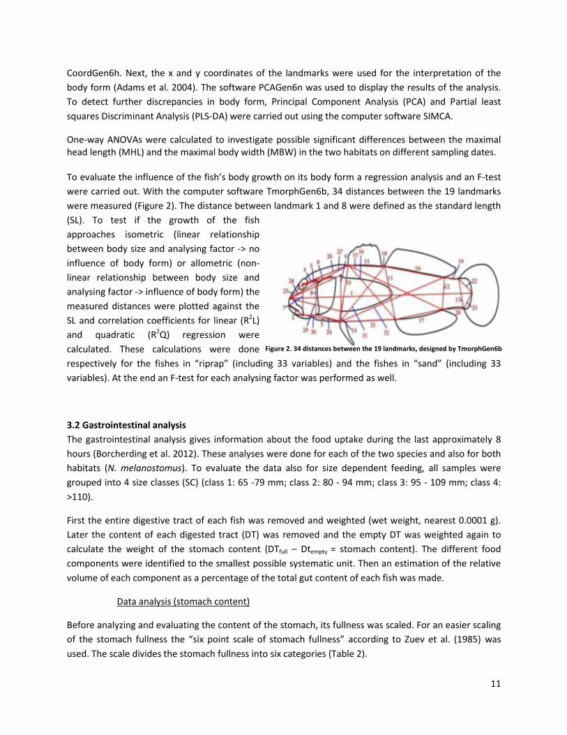
were carried out. With the computer software TmorphGen6b, 34 distances between the 19 landmarks
were measured (Figure 2). The distance between landmark 1 and 8 were defined as the standard length
(SL). To test if the growth of the fish
approaches isometric (linear relationship
between body size and analysing factor -> no
influence of body form) or allometric (non-
linear relationship between body size and
analysing factor -> influence of body form) the
measured distances were plotted against the
SL and correlation coefficients for linear (R2L)
and quadratic (R2Q) regression were
calculated. These calculations were done
respectively for the fishes in “riprap” (including 33 variables) and the fishes in “sand” (including 33
variables). At the end an F-test for each analysing factor was performed as well.
3.2 Gastrointestinal analysis
The gastrointestinal analysis gives information about the food uptake during the last approximately 8
hours (Borcherding et al. 2012). These analyses were done for each of the two species and also for both
habitats (N. melanostomus). To evaluate the data also for size dependent feeding, all samples were
grouped into 4 size classes (SC) (class 1: 65 -79 mm; class 2: 80 - 94 mm; class 3: 95 - 109 mm; class 4:
>110).
First the entire digestive tract of each fish was removed and weighted (wet weight, nearest 0.0001 g).
Later the content of each digested tract (DT) was removed and the empty DT was weighted again to
calculate the weight of the stomach content (DTfull – Dtempty = stomach content). The different food
components were identified to the smallest possible systematic unit. Then an estimation of the relative
volume of each component as a percentage of the total gut content of each fish was made.
Data analysis (stomach content)
Before analyzing and evaluating the content of the stomach, its fullness was scaled. For an easier scaling
of the stomach fullness the “six point scale of stomach fullness” according to Zuev et al. (1985) was
used. The scale divides the stomach fullness into six categories (Table 2).
Figure 2. 34 distances between the 19 landmarks, designed by TmorphGen6b

12
Table 2. Six point scale of stomach fullness according to Zuev et al. (1985)
Category Description
0* Empty
1 Traces of food
2 Filled less than half
3 Filled more than half
4 Full
5 Exclusively cramped *All fishes that were scaled with a 0 and had therefore empty alimentary tracts were not considered in further analysis.
After estimating of the relative volume (in percent) of the different food components the frequency of
occurrence for each component was calculated with the following formula:
F(%) = (fx / f) x 100
F(%) - frequency of occurrence of component x in the studied fish sample
fx - number of fish with component x in food
f - number of all studied fish with full digestive tracts
Next, a one-way ANOVA was done to test if the ratio of each component in the diet of Neogobius
melanostomus differed significantly between the two habitats.
To evaluate the feeding activity of the fish the stomach fullness index (ISF) was calculated:
ISF = (weight of stomach content / weight of the fish) x 100
Schoener’s index was used for calculating the inter- and intraspecific dietary overlap for different
species (N. melanostomus and P. kessleri) and size classes in different habitats (sand; riprap):
S = 1 – ((0.5 ∑|pa - pb|) / 100)
Pa – percentage of food item in species/size class a
Pb – percentage of food item in species /size class b
A Schoener’s diet overlap index above 0.6 is considered as significant (Davis and Todd; 1996).

13
3.3 Analysis of Parasite infection
After the removal of the food content from the digestive tract the content was checked for parasite
infection. If parasites were detected they were identified to the smallest possible systematic unit and
their abundance (individuals) was noted.
Data analysis (parasites)
In the beginning it was tested if the different habitats had an effect on the parasite infection rate of N.
melanostomus (P. kessleri only appeared in one of the two habitats and was therefore excluded from
this analysis). Based on the number of parasites in each individual (Appendix13) a comparison between
the two different habitats (for each sampling date) was done by a one-way ANOVA.
All following analyses were done for both species again.
These analyses started with a grouping of parasites that was based on the transmition of parasites to
the fish by the same invertebrate species. Afterwards the density of the intermediate host in the gut of
infected and non-infected fish was compared by a Mann-Whitney U-test (for all groups of parasites).
This method gives an answer to the question if the fishes are infected because they feed on particular
prey species.
It was also tested if there was a correlation between the number of parasites and the number of intermediate hosts in the diet. This correlation test was done with the help of a one-way ANOVA. This was only done for intermediate hosts which had a significant different density in the stomachs of infected and non-infected fishes.
3.3 Analysis of Gonad development
Finally the gonad somatic index (GSI) was calculated. The GSI can be used to measure the sexual
maturity of fish, describes the relative size of the gonads and is particularly helpful in identifying days
and seasons of spawning (Shaikh et al. 2011; Wootton 1990). According to Belanger (Belanger et al.;
2006) a GSI value below 1% (in males) and below 8% (in females) indicates a non-reproductive status in
N. melanostomus (same values for P. kessleri).
The gonad mass was determined by carefully lifting the gonads with forceps and cutting them out of the
body cavity as close as possible to the origin. Gonads were then weighted to the nearest 0.0001g. It is
important to note that gonads in unmature males are difficult to detect due to their small sizes and they
often weigh less than 0.001g, in this case the gonad somatic index (GSI) is considered 0%.
Data analysis (gonads)
The calculation of the GSI was done as follows:
Body mass – total gonad mass = somatic mass
GSI = (gonad mass / somatic mass) * 100%

14
A one-way ANOVA was done in order to test if the values differed significantly between the two
habitats.
4 Results
4.1 Regression analysis
The regression analysis and the F-test for the individuals of N. melanostomus (sand; riprap) showned
that 20 of the measured variables (61%) can be explained better through linear regression and 13 of the
measured variables (39%) through quadratic regression (Table 3). In both habitats, N. melanostomus
showed the same differentiations (Appendix 4).
Table 3. Regression analysis of 33 different measuring variables (calculated with TmorphGen6b) for N.melanostomus (riprap) plotted against standard length (SL). Correlation coefficient for linear regression (R2L), quadratic regression (R2Q), and best explanation for growth (Q=quadratic; L=linear), n=141.
Number (Fig.2)
Measured variable R2L R2Q F-test Q/L P Best explanation
2 Mouthdepth 0.592 0.595 3.11 ns L 3 Mouth end -VF 0.871 0.872 3.97 ns L 4 Eye –highest spot Po 0.523 0.523 0 ns L 5 Eye –highest spot Op 0.754 0.754 0 ns L 6 Highest spot Po – highest
spot Op 0.580 0.585 5.80 <0.05 Q
7 Eye – mouthend 0.904 0.910 34.52 <0.01 Q 8 Hight Po 0.931 0.936 36.98 <0.01 Q 9 Contact spot VF 0.947 0.947 0 ns L
10 Begin 1D - VF 0.869 0.869 0 ns L 11 Begin 2D – begin AF 0.915 0.917 11.51 <0.01 Q 12 End 2D – end AF 0.928 0.929 6.01 <0.05 Q 13 Contact point VerF 0.921 0.922 5.75 <0.05 Q 14 Contact point PF 0.497 0.497 0 ns L 15 Length 1D 0.815 0.818 7.76 <0.05 Q 16 Length 2D 0.943 0.944 7.99 <0.05 Q 17 Length AF 0.892 0.892 0 ns L 18 End 1D – begin 2D 0.008 0.022 6.65 <0.05 Q
19 End 2D – dorsal contact point VerF
0.447 0.444 2.61 ns L
20 End AF – ventral contact point VerF
0.629 0.639 13.61 <0.01 Q
21 VF – begin AF 0.831 0.834 8.28 <0.05 Q
22 Dorsal contact point VerF - MVerF
0.887 0.888 4.16 ns L
23 Ventral contact point VerF - MVerF
0.879 0.881 8.06 <0.05 Q
15
24 VF – contact point Po/Op 0.804 0.804 0 ns L
25 Upper lip - eye 0.762 0.764 3.89 ns L
26 Eye – begin 1D 0.938 0.938 0 ns L
27 Upper lip – 1D 0.949 0.949 0 ns L
28 Upper lip – dorsal contact point PF
0.888 0.888 0 ns L
29 Upper lip – ventral contact point PF
0.832 0.832 0 ns L
30 Mouth end – contact point Po/Op
0.666 0.667 1.42 ns L
31 Begin 2D - VF 0.889 0.890 4.35 ns L
32 End 2D -VF 0.969 0.969 0 ns L
33 Begin 1D – end AF 0.982 0.982 0 ns L
34 Begin 1D – begin AF 0.947 0.949 15.82 <0.01 Q
The following abbreviations are used: ns (not significant), 1D (first dorsal fin), 2D (second dorsal fin), AF (anal fin), MVerF (middle of vertical
fin), Op (Operculum), PF (Pectoral fin), Po (Praeoperculum), VerF (vertical fin), VF (ventral fin).
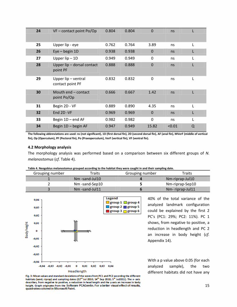
4.2 Morphology analysis
The morphology analysis was performed based on a comparison between six different groups of N.
melanostomus (cf. Table 4).
Table 4. Neogobius melanostomus grouped according to the habitat they were caught in and their sampling date.
Grouping number Traits Grouping number Traits
1 Nm -sand-Jul10 4 Nm-riprap-Jul10 2 Nm -sand-Sep10 5 Nm-riprap-Sep10 3 Nm -sand-Jul11 6 Nm- riprap-Jul11
40% of the total variance of the
analyzed landmark configuration
could be explained by the first 2
PC’s (PC1: 29%; PC2: 11%). PC 1
shows, from negative to positive, a
reduction in headlength and PC 2
an increase in body height (cf.
Appendix 14).
With a p value above 0.05 (for each
analyzed sample), the two
different habitats did not have any
16
0
20
40
60
80
100
1 2 3 4
Fre
qu
en
cy o
f o
ccu
ren
ce in
%
Size classes
Figure 5. Major food categories Nm Sand
Unidentified
Rest
Crustacea
Fish
Chironomidae
Mollusca
0
20
40
60
80
100
1 2 3 4
Fre
qu
en
cy o
f o
ccu
ren
ce in
%
Size classes
Figure 6. Major food categories Nm RipRap
Unidentified
Rest
Crustacea
Fish
Chironomidae
Mollusca
significant influence on changes in the morphology of N. melanostomus (cf. Figure 3). All sample groups
were clustered together with no significant distinguishable differences. The same results were shown by
a Principal component analysis (PCA-X). Partial least squares Discriminant Analysis (PLS-DA) and a
permutation test even showed a random distribution (Appendix 5).
4.3 Gastrointestinal analysis
No sex-dependent differences in condition and stomach fullness were observed within the whole
sample group (Jost Borcherding, pers. comm., August 2012). Therefore, analysis of the condition and
stomach fullness could be made independent of gender.
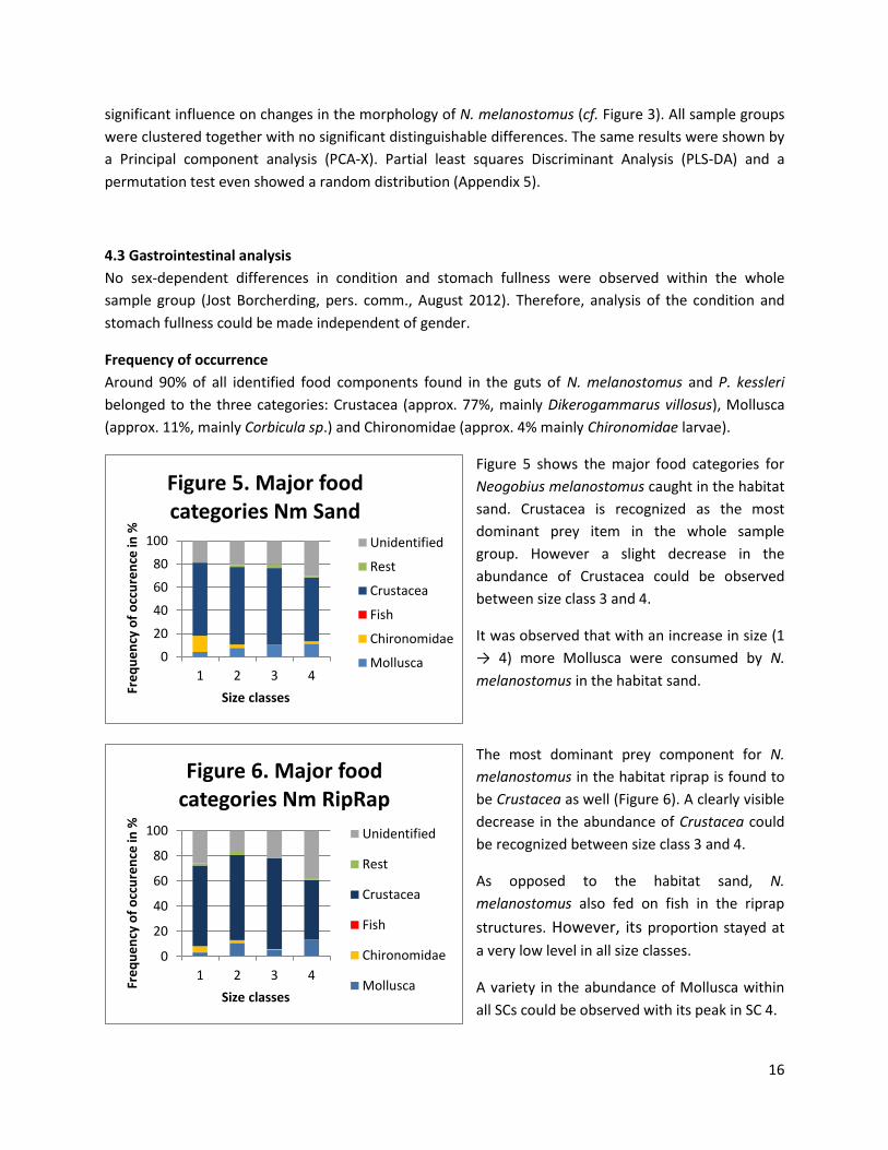
Frequency of occurrence
Around 90% of all identified food components found in the guts of N. melanostomus and P. kessleri
belonged to the three categories: Crustacea (approx. 77%, mainly Dikerogammarus villosus), Mollusca
(approx. 11%, mainly Corbicula sp.) and Chironomidae (approx. 4% mainly Chironomidae larvae).
Figure 5 shows the major food categories for
Neogobius melanostomus caught in the habitat
sand. Crustacea is recognized as the most
dominant prey item in the whole sample
group. However a slight decrease in the
abundance of Crustacea could be observed
between size class 3 and 4.
It was observed that with an increase in size (1
→ 4) more Mollusca were consumed by N.
melanostomus in the habitat sand.
The most dominant prey component for N.
melanostomus in the habitat riprap is found to
be Crustacea as well (Figure 6). A clearly visible
decrease in the abundance of Crustacea could
be recognized between size class 3 and 4.
As opposed to the habitat sand, N.
melanostomus also fed on fish in the riprap
structures. However, its proportion stayed at
a very low level in all size classes.
A variety in the abundance of Mollusca within
all SCs could be observed with its peak in SC 4.
17
0
20
40
60
80
100
1 2 3 4Fre
qu
en
cy o
f o
ccu
ren
ce in
%
Size classes
Figure 7. Major food categories Pk RipRap
Unidentified
Crustacea
Fish
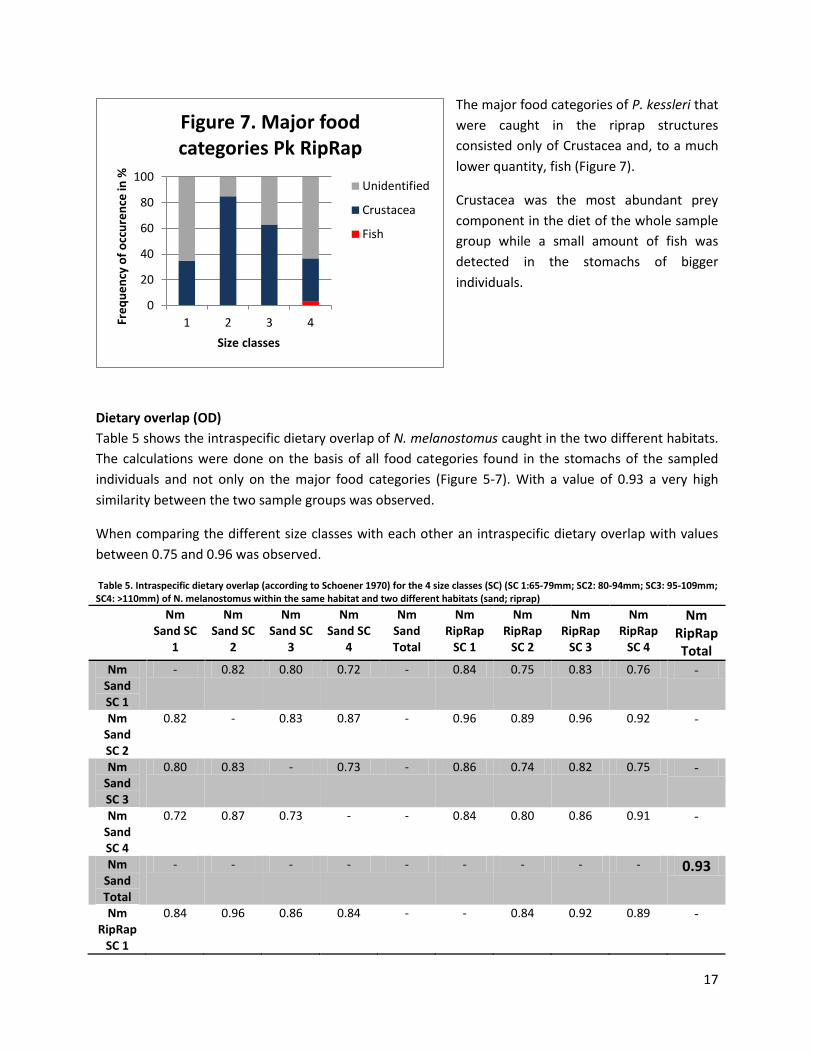
The major food categories of P. kessleri that
were caught in the riprap structures
consisted only of Crustacea and, to a much
lower quantity, fish (Figure 7).
Crustacea was the most abundant prey
component in the diet of the whole sample
group while a small amount of fish was
detected in the stomachs of bigger
individuals.
Dietary overlap (OD)
Table 5 shows the intraspecific dietary overlap of N. melanostomus caught in the two different habitats.
The calculations were done on the basis of all food categories found in the stomachs of the sampled
individuals and not only on the major food categories (Figure 5-7). With a value of 0.93 a very high
similarity between the two sample groups was observed.
When comparing the different size classes with each other an intraspecific dietary overlap with values
between 0.75 and 0.96 was observed.
Table 5. Intraspecific dietary overlap (according to Schoener 1970) for the 4 size classes (SC) (SC 1:65-79mm; SC2: 80-94mm; SC3: 95-109mm; SC4: >110mm) of N. melanostomus within the same habitat and two different habitats (sand; riprap)
Nm
Sand SC 1
Nm Sand SC
2
Nm Sand SC
3
Nm Sand SC
4
Nm Sand Total
Nm RipRap
SC 1
Nm RipRap
SC 2
Nm RipRap
SC 3
Nm RipRap
SC 4
Nm RipRap Total
Nm Sand SC 1
- 0.82 0.80 0.72 - 0.84 0.75 0.83 0.76 -
Nm Sand SC 2
0.82 - 0.83 0.87 - 0.96 0.89 0.96 0.92 -
Nm Sand SC 3
0.80 0.83 - 0.73 - 0.86 0.74 0.82 0.75 -
Nm Sand SC 4
0.72 0.87 0.73 - - 0.84 0.80 0.86 0.91 -
Nm Sand Total
- - - - - - - - - 0.93
Nm RipRap
SC 1
0.84 0.96 0.86 0.84 - - 0.84 0.92 0.89 -

18
Nm RipRap
SC 2
0.75 0.89 0.96 0.92 - 0.84 - 0.90 0.84 -
Nm RipRap
SC 3
0.83 0.96 0.82 0.86 - 0.92 0.90 - 0.91 -
Nm RipRap
SC 4
0.76 0.92 0.75 0.91 - 0.89 0.84 0.91 - -
Nm RipRap Toatl
- - - - 0.93 - - - - -
An interspecific dietary overlap of 0.80 was observed in the riprap structures between N. melanostomus
and P. kessleri (Table 6). Dikerogammarus villosus was the most important prey for both species.
Table 6. Interspecific dieatary overlap (according to Schoener 1970) for P. kessleri and N. Melanostomus (riprap structures)
Stomach Fullness Index (ISF)
The ISF of N. melanostomus did not significantly differ between different sampling dates (p>0.05). These
patterns were observed in both habitats (Table 7).
There were no significant changes observed between the ISF values of N. melanostomus and P. kessleri
(riprap) in September 2010 (p>0.05). Since the sampling size of P. kessleri was very low on the other two
sampling dates, an ANOVA analysis was not made for July 2010 and 2011. A significant higher ISF was
observed in P. kessleri (p<0.05) compared to N. melanostomus in the riprap.
Table 7. Mean, maximum, minimum indexes of stomach fullness (ISF) for N. melanostomus caught in both habitats (riprap; sand) and P. kessleri (riprap) for all sampling dates. n=283.
Date Mean Min Max SD
N. melanostomus Sand
Jul 2010 1.48 0.70 2.56 0.53 Sep 2010 1.52 0.08 4.22 0.79 Jul 2011 2.03 1.13 3.40 0.63
N. melanostomus RipRap
Jul 2010 1.73 0.98 3.20 0.67 Sep 2010 1.79 0.44 4.92 0.88 Jul 2011 1.39 0.85 1.75 0.49
P. kessleri RipRap Jul 2010 2.79 0.48 5.49 1.40 Sep 2010 1.62 0.37 3.14 0.76 Jul 2011 3.15 - - -
Dietary Overlap 0.80
Sum 40.17 Fish 0.83 2.7 1.87 Cladocera 3.33 0 0.38 Dikerogammarus villosus 95 78.37 16.63 Dipteralarve 4.17 0 4.17 Corbicula 12.5 0 12.5 Oligochaeta 1.67 0 1.67

19
4.4 Analysis of Parasite infection
The parasites that were found in the guts of N. melanostomus and P. kessleri in both habitats were
Pomphorhynchus (laevis), Streptocara crassicauda, and Raphidascaris acus.
When comparing the total number of parasites that infected individuals of N. melanostomus in each
habitat the values (cf. Table 8; mean values) were generally higher in the habitat sand than in the riprap
structures on every sampling date. However with a p value above 0.05 for each sampling date, statistical
analyses have shown that the differences between the two habitats were not significant.
Table 8. Number (N) of N. melanostomus infected by Pomphorhynchus (laevis), Streptocara crassicauda, and Raphidascaris acus in each habitat (sand; riprap) for all sampling dates (Jul 2010; Sep 2010; Jul 2011). Furthermore the minimum (min), maximum (max) and mean numbers of parasites (with standard deviation (StDev) for each sampling group.
Sand RipRap
July 2010 N infected individuals 16 8 Min Nparasites 1 1 Max Nparasites 16 9 Mean Nparasites 5.3 3.4
StDev 4.9 0.9
September 2010 N infected individuals 74 74 Min Nparasites 1 1 Max Nparasites 36 35 Mean Nparasites 9.3 8.0
StDev 6.9 7.5
July 2011 N infected individuals 23 35 Min Nparasites 1 1 Max Nparasites 24 32 Mean Nparasites 5.8 4.9
StDev 6.3 5.3
Since it was important for further statistical analysis, possible intermediate hosts for all parasites were
listed. Evaluation had shown that Dikerogammarus villosus can be an intermediate host for either
Pomphorhynchus (laevis) and/or Streptocara crassicauda, while Raphidascaris acus can be transmitted
via several Diptera larvaes and different fishes (cf. Table 9).
Table 9. Evaluation of different macroinvertebrates (as part of the diet of N. melanostomus and P. kessleri) as potential intermediate hosts for Pomphorhynchus (laevis), Streptocara crassicauda, and Raphidascaris acus.
Transmitted parasite
Pomphorhynchus laevis
Streptocara crassicauda
Raphidascaris acus
Intermediate host Oligochaeta No No No Gastropoda No No No Gammarus pulex/ Dikerogammarus villosus
Yes(1) Yes(2) No
Fish No No Yes(3) Diptera (Larvae) No No Yes(4) Corbicula No No No Cladocera No No No
20
(1) Cornet et al. 2009; Choi 2008; (2) Garskavi 1950; (3) Moravec 1994; (4) Moravec 1970
Infected and non-infected individuals
The results for Dikerogammarus villosus showed that there was no significant difference observed
between the density of Dikerogammarus villosus in the stomachs of fishes that were affected by
Pomphorhynchus laevis and/or Streptocara crassicauda (p>0.05). When comparing the density of fish in
the stomachs between the two groups a significant difference was measurable. Individuals that were
infected had a significant higher density of fish in their stomachs than non-infected fish (p<0.01). A
significant difference between infected and non-infected fishes that fed on diptera larvae was not
observed (p>0.05).
Number of parasites and intermediate hosts
Since a significant difference was only measured in the density of fish in the stomachs of infected and
non-infected fishes, this group was the only one tested for a correlation between the number of
parasites and the number of intermediate hosts in their stomachs. There was no correlation between
the number of parasites and the number of intermediate hosts in the fish’s gut (p>0.05).
The highest number of parasites (N=36) in a single stomach was detected in a fish with a stomach that
was filled less than half (category 2). With 15% of all individuals in a single group there were the most
fishes that had more than 20 parasites in their stomachs detected in category 3 (filled more than half).
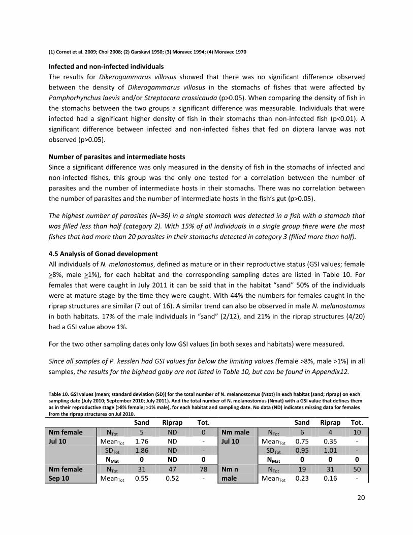
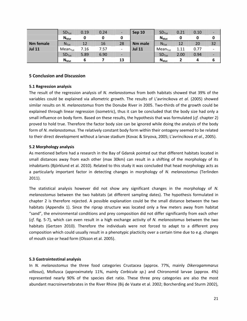
4.5 Analysis of Gonad development
All individuals of N. melanostomus, defined as mature or in their reproductive status (GSI values; female
>8%, male >1%), for each habitat and the corresponding sampling dates are listed in Table 10. For
females that were caught in July 2011 it can be said that in the habitat “sand” 50% of the individuals
were at mature stage by the time they were caught. With 44% the numbers for females caught in the
riprap structures are similar (7 out of 16). A similar trend can also be observed in male N. melanostomus
in both habitats. 17% of the male individuals in “sand” (2/12), and 21% in the riprap structures (4/20)
had a GSI value above 1%.
For the two other sampling dates only low GSI values (in both sexes and habitats) were measured.
Since all samples of P. kessleri had GSI values far below the limiting values (female >8%, male >1%) in all
samples, the results for the bighead goby are not listed in Table 10, but can be found in Appendix12.
Table 10. GSI values (mean; standard deviation (SD)) for the total number of N. melanostomus (Ntot) in each habitat (sand; riprap) on each sampling date (July 2010; September 2010; July 2011). And the total number of N. melanostomus (Nmat) with a GSI value that defines them as in their reproductive stage (>8% female; >1% male), for each habitat and sampling date. No data (ND) indicates missing data for females from the riprap structures on Jul 2010.
Sand Riprap Tot. Sand Riprap Tot.
Nm female Jul 10
NTot 5 ND 0 Nm male Jul 10
NTot 6 4 10 MeanTot 1.76 ND - MeanTot 0.75 0.35 -
SDTot 1.86 ND - SDTot 0.95 1.01 - NMat 0 ND 0 NMat 0 0 0
Nm female Sep 10
NTot 31 47 78 Nm n male
NTot 19 31 50 MeanTot 0.55 0.52 - MeanTot 0.23 0.16 -
21
SDTot 0.19 0.24 - Sep 10 SDTot 0.21 0.10 - NMat 0 0 0 NMat 0 0 0
Nm female Jul 11
NTot 12 16 28 Nm male Jul 11
NTot 12 20 32 MeanTot 7.16 7.57 - MeanTot 1.11 0.77 -
SDTot 5.89 6.90 - SDTot 2.00 0.94 - NMat 6 7 13 NMat 2 4 6
5 Conclusion and Discussion
5.1 Regression analysis
The result of the regression analysis of N. melanostomus from both habitats showed that 39% of the
variables could be explained via allometric growth. The results of L'avrincikova et al. (2005) showed
similar results on N. melanostomus from the Donube River in 2005. Two-thirds of the growth could be
explained through linear regression (isometric), thus it can be concluded that the body size had only a
small influence on body form. Based on these results, the hypothesis that was formulated (cf. chapter 2)
proved to hold true. Therefore the factor body size can be ignored while doing the analysis of the body
form of N. melanostomus. The relatively constant body form within their ontogeny seemed to be related
to their direct development without a larvae stadium (Kovac & Siryova, 2005; L'avrincikova et al., 2005).
5.2 Morphology analysis
As mentioned before had a research in the Bay of Gdansk pointed out that different habitats located in
small distances away from each other (max 30km) can result in a shifting of the morphology of its
inhabitants (Björklund et al. 2010). Related to this study it was concluded that head morphology acts as
a particularly important factor in detecting changes in morphology of N. melanostomus (Terlinden
2011).
The statistical analysis however did not show any significant changes in the morphology of N.
melanostomus between the two habitats (at different sampling dates). The hypothesis formulated in
chapter 2 is therefore rejected. A possible explanation could be the small distance between the two
habitats (Appendix 1). Since the riprap structure was located only a few meters away from habitat
“sand”, the environmental conditions and prey composition did not differ significantly from each other
(cf. fig. 5-7), which can even result in a high exchange activity of N. melanostomus between the two
habitats (Gertzen 2010). Therefore the individuals were not forced to adapt to a different prey
composition which could usually result in a phenotypic placticity over a certain time due to e.g. changes
of mouth size or head form (Olsson et al. 2005).
5.3 Gastrointestinal analysis
In N. melanostomus the three food categories Crustacea (approx. 77%, mainly Dikerogammarus
villosus), Mollusca (approximately 11%, mainly Corbicula sp.) and Chironomid larvae (approx. 4%)
represented nearly 90% of the species diet ratio. These three prey categories are also the most
abundant macroinvertebrates in the River Rhine (Bij de Vaate et al. 2002; Borcherding and Sturm 2002),
22
which illustrates the ability of N. melanostomus to adapt easily to new environments (opportunistic
feeding strategy).
Crustacea was by far the most abundant prey for N. melanostomus in both habitats. It was observed
that towards bigger fishes Mollusca became more important in the species diet. Fish was only part of
the diet of N. melanostomus that were caught in the riprap structures. The differences of food uptake in
the different size classes reflect the results from previous research in the same geographic area
(Borcherding et al. 2012). The overall diet spectrum of N. melanostomus detected in this study
corresponds with observations that were reported before (Polacik et al. 2009; Barton et al. 2005).
The diet of P. kessleri (riprap) consisted mainly of Crustacea and in bigger individuals (>110mm) of an
increased fraction of fish. The observed diet spectrum of P. kessleri in the riprap structures reflected
previous observations made by Borza et al. (2009).
With 93% the intraspecific dietary overlap (according to Schoener 1970) of N. melanostomus in the two
habitats was higher than the interspecific dietary overlap measured between N. melanostomus and P.
kessleri (mean 80%). However both values are very high and as such describe a strong competition for
food sources between the analyzed sample groups (Borcherding et al. 2012; Borza et al. 2009).
According to Salgado et al. (2004) a high dietary overlap between the two species is usually measurable
when they occur together in the same habitat. The highest similarities in the diet of round- and bighead
goby are reported for summer, since high abundances of macro invertebrates in combination with
morphological constraints between both species creates same initial conditions (Borcherding et al. 2012;
Borza et al 2009). Since all samples were taken during summer (July and September) the high dietary
overlap can be related to these results.
The index of stomach fullness (ISF) in N. melanostomus did not show any significant difference between
the two habitats. Since the ISF gives a solid estimation on the quantities of ingested food (Borcherding et
al. 2012), N. melanostomus seemed to have a similar feeding strategy in both habitats due to a similar
proportion of the food components available in the different habitats. Therefore the hypothesis
formulated in chapter 2 can be rejected.
Since the numbers of observations for P. kessleri per sample were not sufficient, statistical comparison
between the two species was not possible for each sampling day individually but only for the September
sample. This analysis did not show a significant difference between ISF values of the two species (Tab.
7). However an overall comparison between ISF values (all sampling dates together) of P. kessleri and N.
melanostomus indicated a significant difference between the two species. P. kessleri had, in nearly every
sample, higher ISF values than N. melanostomus. This fact leads to the conclusion that the hypothesis
formulated in chapter 2 is proved to be correct.
Borcherding et al. (2012) reported that the ISF values in P. kessleri were, without exception, double as
high as in N. melanostomus (over different seasons). However since there were two different methods
used for taking the samples (beach seining (Borcherding et al. 2012); angling) the results reported from
Borcherding et al. are just used to highlight a general trend in the feeding strategy of P. kessleri.
23
ISF values in individuals caught by angling are expected to be low since the fish that is biting the hook is
usually foraging, indicating a stomach that is not completely filled (Gertzen, personal communication
May 2012). However the study has shown that P. kessleri in general had higher ISF values. That could
probably be related to a laboratory experiment on the behavior of the two species that showed that P.
kessleri had always a higher interest in food than N. melanostomus (Borcherding, Hertel, Breiden,
unpublished data).
The results of the gastrointestinal analysis showed that there was a high competition for food resources
between the different size classes of N. melanostomus in both habitats. For the two different species it
can be concluded that a higher demand for food resources of P. kessleri and an interspecific diet overlap
between N. melanostomus and P. kessleri highlighted the competition for food for the two species
(Borza et al., 2009).
5.4 Analysis of Parasite infection
N. melanostomus was infected by three parasite species: larval acanthocephalan Pomphorhynchus laevis
and the larval nematodes Raphidascaris acus and Streptocara crassicauda. Streptocara crassicauda was
only found in N. melanostomus that were caught in the riprap structures. P. kessleri was only infected by
Pomphoryhynchus laevis and Raphidascaris acus.
Statistical analysis of the total abundance of parasites in the two different habitats did not show any
significant difference in the infection rate between sand and the riprap structures. This comparision was
only made for N. melanostomus since P. kessleri only appeared in one of the two habitats.
Since Pomphoryhynchus laevis occur in high densities in main river channels the fact that it was the most
dominant parasite in N. melanostomus and P. kessleri in both habitats is not surprising and matches also
with observations made for the two species in other fresh water habitats (Ondrackova et al. 2009; Kvach
at al. 2007; Molnar 2006; Ondrackova et al. 2006; Kakacheva-Avramova 1983).
This study did not show any significant correlation between parasite infection and a certain prey item.
The only exception was the parasite Raphidascaris acus. Its occurrence was correlated to individuals that
fed on fish. A link between the amount of fish that was consumed and the number of parasites found in
the gut of N. melanostomus and P. kessleri was not detected.
Streptocara crassicauda was found sporadically only in N. melanostomus that was caught in the riprap
structures. S. crassicauda normally affects ducks and other aquatic birds but in its larvae stadium it is
also reported to use N. melanostomus as a reservoir host (Kovalenko 1960;
www.wildpro.twycrosszoo.org). Since all samples were taken during the summer (July; September) and
S. crassicauda is usually found in high densities only in winter (Boughton 1969), a small infection rate in
N. melanostomus by S. crassicauda was not surprising. Next to other abiotic conditions the water
temperature is the constitutive factor for S. crassicauda to be active (Bano et al. 2005). Since the abiotic
conditions that are important for S. crassicauda to be active are the same or really similar the fact that it
was only found in the riprap structure cannot be explained. It seems that the limiting factor was

24
probably sampling size since there were only a few individuals of S. crassicauda. We assume that a
bigger sampling size would also disclose individuals in the sand habitat that were infected by S.
crassicauda.
For the parasite infection in both species, it can finally be concluded that N. melanostomus as well as P.
kessleri can be considered as suitable hosts for a number of parasites found in different habitats in the
Lower Rhine. The importance for the local parasite community can be proved by the fact that most of
the parasites found in the two goby species were in their larvae status, and therefore depended on N.
melanostomus and P. kessleri as an intermediate or paratenic host (Ondračková et al. 2009). This
conclusion shows that the hypothesis that was formulated in chapter 2 is correct.
5.5 Analysis of gonad development
This study showed that the habitat does not have a distinct influence on the reproductive status of N.
melanostomus. The hypothesis formulated in chapter 2 can therefore be rejected. Since the 5th of July
2011 was the only sampling date in which mature individuals were found, special attention has been
paid to this sampling group.
The possible reason why the gonad-development was in a similar progress stage in the two habitats
could be that both, the “sand” and the “riprap” habitat, are located close to each other and offer
therefore similar abiotic factors that are decisive for reproduction. Spawning in N. melanostomus usually
appears in water temperatures from 9 to 26°C (Charlebois et al. 1997). The average water temperature
of the Rhine in July 2011 was 22.5°C (measured in Bad Honnef; www.luadb.lds.nrw.de), which leads to
the conclusion that both habitats offered ideal conditions for reproduction for N. melanostomus.
Low to very low GSI values were detected on the two other sampling dates (22nd July 2010; 14th
September 2010), with maximum individual values around 4 (females) and 0.2 (males) in July 2010 and
values around 0 in both sexes in September 2010.
As batch spawners, females of N. melanostomus release their eggs in portions throughout the spawning
season (2-4 times a year) and not only at one time which gives them an ecological advantage over other
species (Tomczak et al. 2006; www biokids.umich.edu). The reproductive season can last from April until
October (www.caspianenvironment.org) and in general the percentage of reproductive active females
declines in July and increases in October for a short time again (Macinnis et al. 2000). Macinnis et al.
(2000) studied the Upper Detroit River and reported that most females of the round goby have high GSI
values in May, June and early July. Later in July the mean GSI values decrease normally and reach
seldom more than 5% by the end of July. In September the GSI values usually even out around 0%. The
observations made in the Upper Detroit River match with the results of this study regarding all sample
dates. Females with increased GSI values around 4% were found in the samples taken in July 2010. In
September 2010 all GSI values of female N. melanostomus were around 0.

25
The reproduction cycle of male N. melanostomus lasts from early March until early September (Tomczak
et al. 2006). Males with high GSI values are normally observed in April until May, June until early July
and August, depending on the water temperature. In late July and September values are normally very
low (cf. females). The same observation was made in this study. Males had low GSI values in July 2010
and in September many individuals were detected that had values close to or equal 0%.
A possible answer to the question why only half of the female population and 1/5th of the male
population of N. melanostomus were mature in 2011 could be related to another study made in the
middle Danube that was published in early 2012 by Grula et al. . The results of this study pointed out
that all specimens of N. melanostomus bigger than 61mm (SL) and older than 2.5 years can be
considered as mature. Regarding the size of the fishes that were analyzed can be said that around 25%
of females (7/28) and around 10% of males (3/32) had a body size equal or below this value and were
therefore not mature. Another explanation could be that the fishes in the sample with GSI values below
8% (female) respectively 1% (male) had already spawned or were shortly before the stage of being
defined as mature.
6 Final conclusion
In this study we compared two habitats that offered different environmental conditions. The goal was to
determine if differences in soil structure (sand and gravel; riprap structures) have an influence on the
two Gobiid species Ponticola kessleri and Neogobius melanostomus regarding changes in their
morphology, feeding characteristics, gonad development and/or parasite infection.
The study showed that the two different habitats did not have any significant influence on any of the
studied traits. This could probably be related to a high similarity in the biotic (e.g. dietary overlap of 80%
and more) and abiotic (water temperature, etc.) conditions in both habitats due to only a small distance
between the two habitats. The morphology analysis indicated that N. melanostomus regularly moves
within the two habitats. A high dietary overlap did not only indicate same food sources in both habitats
but also a high competition between N. melanostomus and P. kessleri for these food items.

26
Acknowledgements
I would like to express special thanks to:
…PD Dr. Jost Borcherding for providing this thesis, his useful feedbacks and extensive support … Anna Brunberg and Philipp Hirsch for their support and forging the links between Cologne and
Uppsala
… Peter Eklöv who helped me to enjoy statistics the way he does
… Sebastian Sobek for sharing his knowledge according PCA analysis with me
… PH Dr. Pavel and Mgr. Marketa Ondrackova who taught me how nice it can be to work with parasites
… Svenja Gertzen and Sylvia Breiden who supported me during this research with their knowledge and
made the time of my research so unforgettable for me
… Jovanna Kovacic for supporting me with her knowledge and experience
… Elke Hohenadler und Luise Jagemann who always motivated and supported me unconditionally during my entire studies … and last but not least a special thanks goes to David John Yabis who became my personal tower of
strength with his continuous support, motivation and help during the past two years.
References
Adams, D. C., F. J. Rohlf, and D. E. Slice (2004). "Geometric morphometrics: ten years of progress
following the 'revolution'." Italian Journal of Zoology 71 (1), pp. 5-16.
Adamek, Z., Andreji, J., and Gallardo, J. M. (2007). "Food habits of four bottom-dwelling gobiid species at
the confluence of the Danube and hron rivers (South slovakia)." International Review of Hydrobiology,
92(4-5), pp. 554-563.
Ahnelt, H., Banarescu, P., Spolwind, R., Harka, A., and Waidbacher, H. (1998). "Occurrence and
distribution of three gobiid species (Pisces, Gobiidae) in the middle and upper Danube region - examples
of different dispersal patterns?" Biologia, 53(5), pp. 665-678.
Barton, D.R., Johnson, R.A., Campbell, L., Petruniak, J., Patterson, M. (2005). „Effects of round gobies
(Neogobius melanostomus) on dreissenid mussels and other invertebrates in eastern Lake Erie, 2002–
2004.“ J. Great Lakes Res. 31, pp. 252–261.
Belanger, R.M., and Corkum, L.D., (2003). „Susceptibility of tethered round gobies (Neogobius melanostomus) to predation in habitats with and without Shelters.“ J. Great Lakes Res. 29 (4), pp. 588-593.

27
Belanger, R. M., Corkum, L. D., Li, W. & Zielinski, B. S. (2006). ”Olfactory sensory input increases gill ventilation in male round gobies (Neogobius melanostomus) during exposure to steroids.” Comparative Biochemistry and Physiology A 144, pp. 196–202. Bij de Vaate, A., Jazdzewski, K., Ketelaars, H.A.M., Gollasch, S., Van der Velde, G. ( 2002). ”Geographical patterns in range extension of Ponto-Caspian macroinvertebrate species in Europe.” Can. J. Fish. Aquat. Sci. 59, pp. 1159–1174.
Björklund, M. and G. Almqvist (2010) "Rapid spatial genetic differentiation in an invasive species, the round goby Neogobius melanostomus in the Baltic Sea." Biological Invasions 12 (8), pp. 2609-18. Borcherding, J., Dolina, M., Heermann, L., Knutzen, P., Krüger, S., Treeck v., R., Gertzen, S. (accepted 2012, in press). “Feeding and niche differentiation in three invasive gobies in the Lower Rhine, Germany”. Borcherding, J., Staas, S., Krüger, S., Ondračková, M., Šlapanský, L., Jurajda, P. (2011). “Non-native Gobiid species in the lower River Rhine (Germany): recent range extensions and densities.” Journal of Applied Ichthyology 27(1), pp. 153–155. Borcherding, J., Sturm, W. (2002). „The seasonal succession of macroinvertebrates, in particular the zebra mussel (Dreissena polymorpha), in the River Rhine and two neighbouring gravel-pit lakes monitored using artificial substrates.“ Int. Rev. Hydrobiol. 87, pp. 165–181. Borza, P., Erös, T., Oertel, N. (2009). „Food resource partitioning between two invasive Gobiid species (Pisces, Gobiidae) in the littoral zone of the River Danube, Hungary.“ Int. Rev. Hydrobiol. 94, pp. 609–621. Boughton, E. (1969). „On the Occurrence of Oesophageal Worms, Streptocara crassicauda, in
Ornamental Ducks in Hampshire“. Journal of Helminthology / Volume 43 / Issue 34, pp. 273 280.
Capova, M., Zlatnicka, I., Kovac, V., and Katina, S. (2008). "Ontogenetic variability in the external
morphology of monkey goby, Neogobius fluviatilis (Pallas, 1814) and its relevance to invasion potential."
Hydrobiologia, 607, pp. 17-26.
Carman, S.M., Janssen, J., Jude, D. J., Berg, M. B. (2006). „Diel interactions between prey behaviour and feeding in an invasive fish, the round goby, in a North American river.“ Freshwater Biology 51, pp. 742–755. Copp, G. H., Kovac, V., Zweimüller, I., Dias, A., Nascimento, M., and Balazova, M. (2008). "Preliminary
study of dietary interactions between invading Ponto-Caspian gobies and some native fish species in the
River Danube near Bratislava (Slovakia)." Aquat. Invas., 3(2), pp. 193-200.
Corkum, L.D., Sapota, M. R., Skora, K. E. (2004). „The round goby, Neogobius melanostomus, a fish invader on both sides of the Atlantic Ocean.“ Biological Invasions 6,pp. 173-181. Cornet, S., Franceschi, N., Bollache, L., Rigaud, L., Sorci, G. (2009). „Variation and covariation in infectivity, virulence and immunodepression in the host–parasite association Gammarus
28
pulex–Pomphorhynchus laevis“. Proc. R. Soc. B 2009 276, pp. 4229-4236. Davis BM, Todd TN (1996). “Competition between larval lake herring (Coregonus artedi) and lake whitefish (Coregonus clupeaformis) for zooplankton.” Can. J. Fish. Aqaut. Sci. 55, pp. 1140-1148.
Dubs, D. O. L., and Corkum, L. D., (1996). "Behavioral interactions between round gobies (Neogobius
melanostomus) and mottled sculpins (Cottus bairdi)." Journal of Great Lakes Research, 22(4), pp. 838-
844.
Eros, T., Sevcsik, A., and Toth, B. (2005). "Abundance and night-time habitat use patterns of Ponto-
Caspian gobiid species (Pisces, Gobiidae) in the littoral zone of the River Danube, Hungary." Journal of
Applied Ichthyology, 21(4), pp. 350-357.
Forseth, T., Helland, I. P., Eklöv, P., Fiske, P., Ugedal, O., Hindar, K., Karlsson, St, Einum, S., Diserud, O.,
Fleming, I. A. (not published yet). „Character Divergence in Brown Trout (Salmo trutta) due to
Competition from Atlantic Salmon (Salmo salar)“
Garkavi, B. L. (1950). „Reservoir hosts of Streptocara crassicauda (Creplin, 1829) Skryabin, 1915, a
parasite of domestic ducks.“ , Trudy Vsesoyuznogo Instituta Gel'mintologii Imeni Akademika K. I.
Skryabina. 1950 Vol. 4, pp. 5-7.
Gertzen, S. (2010). “Habitat partitioning in three invasive gobiid species in the Lower Rhine.” Master
thesis University of Cologne, Germany, p. 3
Gruľa, D., Balážová, M., Copp, G.H., Kováč, V. (2012) “Age and growth of invasive round goby Neogobius
melanostomus from middle Danube.” Central European Journal of Biology, 7(3), pp. 448-459
Heermann, L., Eriksson, L. O., Magnhagen, C., Borcherding, J. (2009). “Size-dependent energy storage and winter mortality of perch”. Ecology of Freshwater Fish, 18: pp. 560–571.
Johnson, T. B., Allen, M., Corkum, L. D., and Lee, V. A. (2005). "Comparison of methods needed to
estimate population size of round gobies (Neogobius melanostomus) in western Lake Erie." Journal of
Great Lakes Research, 31(1), pp. 78-86.
Kakacheva-Avramova, D., (1983). “Helminths of freshwater fishes in Bulgaria.” Publishing House of the
Bulgarian Academy of Sciences, Sofia.
Karlson, A. M. L., Almqvist, G., Skora, K. E., and Appelberg, M. (2007). "Indications of competition
between non-indigenous round goby and native flounder in the Baltic Sea." Ices Journal of Marine
Science, 64(3), pp. 479-486.
Keeley, E. R., Parkinson, E. A., Taylor, E. B: (2007). „The origins of ecotypic variation of rainbow trout: a
test of environmental vs genetically based differences in morphology.“ J. Evol. Biol. 20, pp. 725-36
Kolar, C. S. and Lodge, D. M. (2002). „Ecological predictions and risk assessment for alien fishes in North America.“ Science 298, pp. 1233-1236.

29
Kornis, M. S., Mercado-Silva, N., Vander Zanden, M. J. (2011). ”Twenty years of invasion: a review of round goby.” Journal of Fish Biology (2012) 80, pp. 235–285. Kovac, V., Copp, G. H., and Sousa, R. P. (2009). "Life-history traits of invasive bighead goby Neogobius
kessleri (Gunther, 1861) from the middle Danube River, with a reflection on which goby species may win
the competition." Journal of Applied Ichthyology, 25(1), pp. 33-37.
Kovac, V., Siryova, S. (2005). „Ontogenetic variability in external morphology of bighead goby Neogobius kessleri from the Middle Danube, Slovakia.“ J. Appl. Ichthyol. 21, pp. 312-315. Kovalenko, I., I. ( 1960). "Study of the life cycle of some helminths of domestic ducks from farms on the Azov coast." Dokl. Akad. Nauk S.S.S.R., 133, pp. 1259-1261. Kvach, Y., Skora, K. E. (2007). „Metazoa parasites of the invasive round goby Apollonia melanostoma (Neogobius melanostomus) (Pallas) (Gobiidae: Osteichthyes) in the Gulf of Gdansk, Baltic Sea, Poland: a comparison with the Black Sea.“ Parasitol Res 100, pp.767–774. L'avrincikova, M., Kovac, V.,Katina, S. (2005). "Ontogenetic variability in external morphology of round goby Neogobius melanostomus from Middle Danube, Slovakia." Journal of Applied Ichthyology 21 (4), pp. 328-34. Macinnis, A.J., Corkum, L.D. (2000). „Fecundity and Reproductive Season of the Round Goby Neogobius melanostomus in the Upper Detroit River.“ Transactions of the American Fisheries Society 129, pp.136–144. Miller, P.J., (1984). The tokology of gobioid fishes. In: Potts, G.W., Wootton, R.J. (Eds.), Fish
reproduction: strategies and tactics. Wootton Academic Press, London, pp. 119–153.
Molnar, K. (2006). “Some remarks on parasitic infections of the invasive Neogobius spp. (Pisces) in the
Hungarian reaches of the Danube River, with a description of Goussia szekelyi sp.n. (Apicomplexa:
Eimeriidae).” J Appl Ichthyol 22, pp.395–400.
Moravec, F. (1994). “Parasitic nematodes of freshwater fishes of Europe.” Academia, Prague.
Moravec, F. (1970). “Studies on the development of Raphidascaris acus (Bloch, 1779) (Nematoda:
Heterocheilidae).” Vestnik Ceskoslovenske Spolecnosti Zoologicke Vol. 34 No. 1, pp. 33-49.
Olsson, J., Eklöv, P. (2005). „Habitat structure, prey type and morphological reversibility: factors
influencing phenotypic plasticity in perch“. Evolutionary Ecology and Research2 7: pp. 1-15.
Ondrackova, M., Trichkova, T., Jurajda, P. (2006). “Present and historical occurrence of metazoan
parasites in Neogobius kessleri (Gobiidae) in the Bulgarian section of the Danube River.” Acta Zool Bulg
58, pp. 399–406.
Ondrackova, M., Davidova, M., Blazek, R., Gelnar, M., Jurajda, P. (2009). ”The interaction between an
introduced fish host and local parasite fauna: Neogobius kessleri in the middle Danube River”. Parasitol
Res 105, pp.201–208.

30
Polacik, M., Janac, M., Jurajda, P., Adamek, Z., Ondrackova, M., Trichkova, T., Vassilev, M. (2009).
”Invasive gobies in the Danube: invasion success facilitated by availability and selection of superior food
resources.” Ecol. Freshwat. Fish 18, pp. 640–649.
Pimentel, D., McNair, S., Janecka, J., Wightman, J., Simmonds, C., O’Connell, C., Wong, E., Russel, L., Zern, J., Aquino, T., Tsomondo, T. (2001). “Economic and environmental threats of alien plant, animal, and microbe invasions.” Agriculture, Ecosystems & Environment, Volume 84, Issue 1, pp. 1-20. Price, D. T., Qvamström, A., Irwin, D. E. (2003). „The role of phenotypic plasticity in driving genetic evolution.“ Proc Biol Sci volume 270, pp. 1433-39. Ray, W.J. and Corkum, L.D. (2001). „Habitat and site affinity of the round goby.“ J. Great Lakes Res. 27 (3), pp. 329-334. Reid, D., and Orlova, M. (2002). "Geological and evolutionary underpinnings for the success of Ponto-
Caspian species invasions in the Baltic Sea and North American Great Lakes." Canadian Journal of
Fisheries and Aquatic Sciences, 59(7), pp. 1144-1158.
Ricciardi, A., MacIsaac, H.J. (2000).” Recent mass invasion of the North American Great Lakes by Ponto–Caspian species.” TREE vol. 15, no. 2 February 2000, pp. 62-65 Salgado, J.P., Cabral, H.N., Costa, M.J. (2004). “Feeding ecology of the gobies Pomatoschistus minutus (Pallas 1770) and Pomatoschistus microps (Kroyer, 1838) in the upper Tagus estuary, Portugal.” Sci. Mar. 68, pp. 425–434. Sapota, M.R. (2004). „The round goby (Neogobius melanostomus) in the Gulf of Gdańsk – a species introduction into the Baltic Sea.“ Hydrobiologia 514, pp. 219-224. Schoener, T.W. (1970). “Nonsynchronous spatial overlap of lizards in patchy habitats.” Ecology 51, pp. 408–418. Shaikh A. S., Prakash S. L. (2011). “Biochemical Composition and Gonadosomatic Index of Three Major Carps in Hatnoor Reservoir, Maharashtra, India.” Journal of Ecobiotechnology 2011, 3(6), pp.01-04
Smith, T. B., Skulason, S. (1996) ”Evolutionary significance of resource polymorphisms in fishes,
amphibians, and birds” Annu. Rev. Ecol. Syst. 27, 00. 111-33
Strayer, D. L., Eviner, V. T., Jeschke, J. M., and Pace, M. L. (2006). "Understanding the long-term
effects of species invasions." Trends in Ecology & Evolution, 21(11), pp. 645-651.
Tomczak M., T., Sapota, M.R. (2006). ”The fecundity and gonad development cycle of the round goby
(Neogobius melanostomus Pallas 1811) from the Gulf of Gdańsk.” Oce.Hydr.Stud. Vol. XXXV, No.4, pp.
353-367
Terlinden, C. (2011). ” Morphologische Untersuchungen an der invasiven Schwarzmaulgrundel
(Neogobius melanostomus Pallas, 1811) in unterschiedlichen Habitaten der Danziger Bucht.” Master
thesis University of Cologne, Germany

31
van Beek, G. C. W. (2006). "The round goby Neogobius melanostomus first recorded in the
Netherlands." Aquat. Invas., 1(1), pp. 42-43.
Vanderploeg, H.A., Nalepa, T. F., Jude, D. J., Mills, E. L., Holeck, K. T., Liebig, J. R., Grigorovich, I. A., Ojaveer, H. (2002). „Dispersal and emerging ecological impacts of Ponto- Caspian species in the Laurentian Great Lakes.“ Can. J. Fish. Aquat. Sci. 59, pp. 1209-1228.
Walsh, M.G., Dittman, D. E., O’Gorman, R. (2007). „Occurrence and food habits of the round goby in the profundal zone of southwestern Lake Ontario.“ J. Great Lakes Res. 33, pp. 83-92. Wiesner, C. (2005). "New records of non-indigenous gobies (Neogobius spp.) in the Austrian Danube."
Journal of Applied Ichthyology, 21(4), pp. 324-327.
Wootton, R.J. (1990). „Ecology of teleost fishes.“ Chapman & Hall, London
Zuev, G.V., Nigmatullin, C. M., Nikolsky, V. N. (1985). „Nektonic oceanic squids (Genus
Sthenoteuthis)“, Agropromizdat Publishing House, Moscow, p. 224
Websites:
Environment Canada; https://www.ec.gc.ca/eee-ias/default.asp?lang=En&n=4612AC81-1; 4.08.2012
Invasive Species Specialist Group ©2008; http://www.issg.org/is_what_are_their_impacts.htm;
2.08.2012
Landesamt fuer Natur, Umwelt und Verbraucherschutz Nordrhein Westfalen;
http://luadb.lds.nrw.de/LUA/wiski/pegel.php; 3.07.2012
MarineBio ©1998-2012; http://marinebio.org/Oceans/Conservation/Moyle/ch10.asp; 3.08.2012
Natureserve ©2010; http://www.natureserve.org/consIssues/invasivespecies.jsp; 2.08.2012
Stepanova T.G., CaspNIRKh, Astrakhan, Russia;
http://www.caspianenvironment.org/biodb/eng/fishes/Neogobius%20melanostomus/main.htm;
4.09.2012
University of Michigan; http://www.biokids.umich.edu/critters/Neogobius_melanostomus/; 4.09.2012
US-CGNET; http://www.fishbase.us/summary/Neogobius-kessleri.html; 2.09.2012
Wildpro;
http://wildpro.twycrosszoo.org/S/0zANe_Secernente/Spir_Acua_Streptocara/Streptocara_crassicauda.h
tm; 2.08.2012
Articles:
Choi, C. Q. (2007). “Parasitic Worms Alter Hosts' Sense of Smell to Better Its Lot in Life”, Fox News, Life
Science. Retrieved 2008-07-03

32
Appendix
Appendix 1: Sampling spots
Habitat Riprap (A) and Riprap (B)
Fig. A1: Map of river Rhine (km 842) with the two different angling spots (Riprap, A; Sand,B) Fig. A2: Map of Germany, angling spot
marked (http://weltkarte.com)

33
Appendix 2: Raw Data Tab. A: Raw data of the two species N. melanostomus (Nm) and P. kessleri (Pk) caught in two different habitats (sand; riprap) in the Lower Rhine, Germany on the 22nd July 2010
Fish ID
Date Habitat Spezies Sex TL (mm)
Fish weight
(g)
Stomach full (g)
Stomach empty
(g)
MHW (mm)
MBW (mm)
Mouth (mm)
S.content Weight (g)
Corrected Condition
(K)
96 22.07.10 RipRap Nm f 122 27,88 0,92 0,65 21,03 20,14 8,34 0,27 1,52
100 22.07.10 RipRap Nm f 76 6,97 0,28 0,15 11,01 10,11 5,53 0,13 1,56
101 22.07.10 RipRap Nm m 75 6,65 0,15 0,06 10,82 9,87 5,43 0,09 1,55
102 22.07.10 RipRap Nm f 76 6,10 0,15 0,06 10,88 9,57 5,38 0,09 1,37
103 22.07.10 RipRap Nm m 85 9,18 0,27 0,17 11,08 10,72 6,74 0,10 1,48
106 22.07.10 RipRap Nm m 110 24,69 0,95 0,65 20,8 18,43 8,72 0,31 1,83
107 22.07.10 RipRap Nm m 75 6,88 0,30 0,07 10,5 9,89 6,76 0,23 1,58
108 22.07.10 RipRap Nm m 85 8,91 0,34 0,18 12,15 10,74 6,88 0,16 1,42
196 22.07.10 RipRap Nm f 79 9,23 0,27 0,05 12,03 11,09 7,76 0,22 1,83
197 22.07.10 RipRap Nm f 124 35,83 1,54 0,45 21,84 19,52 10,3 1,09 1,82
198 22.07.10 RipRap Nm m 97 14,80 0,45 0,27 15,83 14,37 8,43 0,18 1,60
199 22.07.10 RipRap Nm f 72 7,51 0,20 0,03 11,92 10,98 7,65 0,17 1,97
91 22.07.10 RipRap Pk f 131 32,05 1,42 1,15 22,55 20,16 9,83 0,27 1,41
92 22.07.10 RipRap Pk m 116 19,11 0,72 0,38 19,23 16,99 7,34 0,33 1,20
109 22.07.10 Riprap Pk f 108 15,55 0,49 0,34 17,35 16,19 8,35 0,15 1,22
89 22.07.10 Sand Nm f 88 9,89 0,25 0,11 12,03 10,76 4,47 0,15 1,43
90 22.07.10 Sand Nm m 103 17,42 0,93 0,47 16,77 15,96 6,53 0,46 1,55
93 22.07.10 Sand Nm m 94 12,38 0,47 0,25 12,89 12,03 6,99 0,22 1,46
94 22.07.10 Sand Nm 80 7,85 0,27 0,14 11,93 11,07 5,42 0,13 1,51
95 22.07.10 Sand Nm f 72 5,15 0,16 0,10 9,95 8,75 5,71 0,06 1,36
97 22.07.10 Sand Nm m 79 6,84 0,23 0,14 10,32 8,98 5,54 0,08 1,37
98 22.07.10 Sand Nm m 97 13,89 0,47 0,21 14,41 12,27 7,28 0,27 1,49
99 22.07.10 Sand Nm f 84 8,66 0,32 0,19 11,43 10,84 5,69 0,13 1,44
104 22.07.10 Sand Nm m 81 8,37 0,23 0,09 12,01 11,22 5,61 0,15 1,55
105 22.07.10 Sand Nm m 107 19,70 0,67 0,41 17,59 15,77 8,12 0,26 1,59
110 22.07.10 Sand Nm f 68 5,39 0,17 0,11 9,93 8,73 5,73 0,06 1,70
111 22.07.10 Sand Nm f 70 6,37 0,28 0,13 10,32 9,65 6,01 0,15 1,81
112 22.07.10 Sand Nm m 119 35,20 0,77 0,52 21,27 20,28 12 0,24 2,07
Tab. B: Raw data of the two species N. melanostomus (Nm) and P. kessleri (Pk) caught in two different habitats (sand; riprap) in the Lower Rhine, Germany on the 14th September 2010
Fish ID
Date Habitat Spezies Sex TL (mm)
Fish weight (g)
Stomach full (g)
Stomach empty
(g)
MHW (mm)
MBW (mm)
Mouth (mm)
S.content Weight
(g)
Corrected Condition
(K)
26 14.09.10 RipRap Nm f 91 11,00 0,57 0,31 14,32 13,53 4,51 0,26 1,43
27 14.09.10 RipRap Nm m 85 8,60 0,27 0,13 12,58 11,94 4,48 0,14 1,38
41 14.09.10 RipRap Nm m 96 17,60 0,76 0,44 16,12 14,88 7,69 0,32 1,95
43 14.09.10 RipRap Nm m 109 25,55 0,45 0,32 19,72 17,84 6,74 0,13 1,96

34
Fish ID
Date Habitat Spezies Sex TL (mm)
Fish weight (g)
Stomach full (g)
Stomach empty
(g)
MHW (mm)
MBW (mm)
Mouth (mm)
S.content Weight
(g)
Corrected Condition
(K)
44 14.09.10 RipRap Nm m 103 20,69 0,88 0,47 18,25 17,04 7,77 0,41 1,86
45 14.09.10 RipRap Nm m 94 14,14 0,49 0,29 16,06 15,88 6,34 0,20 1,68
46 14.09.10 RipRap Nm m 91 12,04 0,51 0,27 14,78 13,41 5,37 0,24 1,57
47 14.09.10 RipRap Nm m 99 15,53 0,53 0,37 15,93 15,23 6,22 0,16 1,58
48 14.09.10 RipRap Nm m 90 10,82 0,27 0,18 14,49 13,58 6,13 0,09 1,47
50 14.09.10 RipRap Nm m 86 9,89 0,43 0,19 13,15 12,88 6,13 0,23 1,52
53 14.09.10 RipRap Nm f 79 7,66 0,19 0,08 12,75 11,38 4,68 0,10 1,53
54 14.09.10 RipRap Nm f 75 6,96 0,20 0,10 10,71 10,16 5,03 0,10 1,63
55 14.09.10 RipRap Nm f 85 9,06 0,22 0,11 13,26 11,73 5,64 0,11 1,46
56 14.09.10 RipRap Nm m 90 11,20 0,37 0,19 13,83 12,79 5,55 0,18 1,51
57 14.09.10 RipRap Nm m 120 27,84 0,92 0,43 21,29 17,59 8,46 0,49 1,58
58 14.09.10 RipRap Nm f 99 14,55 0,39 0,19 16,98 13,68 6,42 0,20 1,48
59 14.09.10 RipRap Nm m 102 19,64 0,85 0,58 17,8 15,32 7,63 0,27 1,83
60 14.09.10 RipRap Nm f 128 29,39 1,37 0,70 20,87 19,7 8,67 0,67 1,37
62 14.09.10 RipRap Nm m 100 14,82 0,62 0,19 15,22 14,66 6,76 0,43 1,44
65 14.09.10 RipRap Nm m 110 21,38 0,56 0,29 17,63 16,81 6,11 0,28 1,59
69 14.09.10 RipRap Nm m 95 14,15 0,31 0,16 14,39 13,11 5,52 0,15 1,63
70 14.09.10 RipRap Nm f 88 9,57 0,17 0,10 12,55 11,01 4,89 0,07 1,39
71 14.09.10 RipRap Nm m 84 8,52 0,36 0,12 11,43 10,88 4,33 0,24 1,40
72 14.09.10 RipRap Nm m 78 6,41 0,20 0,10 10,83 9,93 4,25 0,11 1,33
73 14.09.10 RipRap Nm f 89 11,95 0,24 0,12 14,39 13,14 4,87 0,12 1,68
74 14.09.10 RipRap Nm m 91 10,86 0,25 0,10 14,71 13,19 5,59 0,15 1,42
75 14.09.10 RipRap Nm f 79 6,50 0,10 0,06 10,96 10,17 5 0,04 1,31
113 14.09.10 RipRap Nm f 96 18,83 0,40 0,30 15,89 14,55 7,03 0,10 2,12
113 14.09.10 RipRap Nm f 72 5,60 0,26 0,12 10,81 10,2 5,09 0,14 1,46
114 14.09.10 RipRap Nm m 112 25,23 0,76 0,41 19,03 17,76 6,94 0,35 1,77
115 14.09.10 RipRap Nm f 78 7,64 0,16 0,11 11,28 10,4 6,98 0,05 1,60
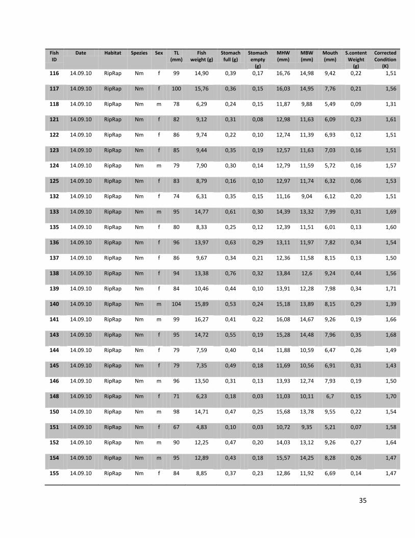
35
Fish ID
Date Habitat Spezies Sex TL (mm)
Fish weight (g)
Stomach full (g)
Stomach empty
(g)
MHW (mm)
MBW (mm)
Mouth (mm)
S.content Weight
(g)
Corrected Condition
(K)
116 14.09.10 RipRap Nm f 99 14,90 0,39 0,17 16,76 14,98 9,42 0,22 1,51
117 14.09.10 RipRap Nm f 100 15,76 0,36 0,15 16,03 14,95 7,76 0,21 1,56
118 14.09.10 RipRap Nm m 78 6,29 0,24 0,15 11,87 9,88 5,49 0,09 1,31
121 14.09.10 RipRap Nm f 82 9,12 0,31 0,08 12,98 11,63 6,09 0,23 1,61
122 14.09.10 RipRap Nm f 86 9,74 0,22 0,10 12,74 11,39 6,93 0,12 1,51
123 14.09.10 RipRap Nm f 85 9,44 0,35 0,19 12,57 11,63 7,03 0,16 1,51
124 14.09.10 RipRap Nm m 79 7,90 0,30 0,14 12,79 11,59 5,72 0,16 1,57
125 14.09.10 RipRap Nm f 83 8,79 0,16 0,10 12,97 11,74 6,32 0,06 1,53
132 14.09.10 RipRap Nm f 74 6,31 0,35 0,15 11,16 9,04 6,12 0,20 1,51
133 14.09.10 RipRap Nm m 95 14,77 0,61 0,30 14,39 13,32 7,99 0,31 1,69
135 14.09.10 RipRap Nm f 80 8,33 0,25 0,12 12,39 11,51 6,01 0,13 1,60
136 14.09.10 RipRap Nm f 96 13,97 0,63 0,29 13,11 11,97 7,82 0,34 1,54
137 14.09.10 RipRap Nm f 86 9,67 0,34 0,21 12,36 11,58 8,15 0,13 1,50
138 14.09.10 RipRap Nm f 94 13,38 0,76 0,32 13,84 12,6 9,24 0,44 1,56
139 14.09.10 RipRap Nm f 84 10,46 0,44 0,10 13,91 12,28 7,98 0,34 1,71
140 14.09.10 RipRap Nm m 104 15,89 0,53 0,24 15,18 13,89 8,15 0,29 1,39
141 14.09.10 RipRap Nm m 99 16,27 0,41 0,22 16,08 14,67 9,26 0,19 1,66
143 14.09.10 RipRap Nm f 95 14,72 0,55 0,19 15,28 14,48 7,96 0,35 1,68
144 14.09.10 RipRap Nm f 79 7,59 0,40 0,14 11,88 10,59 6,47 0,26 1,49
145 14.09.10 RipRap Nm f 79 7,35 0,49 0,18 11,69 10,56 6,91 0,31 1,43
146 14.09.10 RipRap Nm m 96 13,50 0,31 0,13 13,93 12,74 7,93 0,19 1,50
148 14.09.10 RipRap Nm f 71 6,23 0,18 0,03 11,03 10,11 6,7 0,15 1,70
150 14.09.10 RipRap Nm m 98 14,71 0,47 0,25 15,68 13,78 9,55 0,22 1,54
151 14.09.10 RipRap Nm f 67 4,83 0,10 0,03 10,72 9,35 5,21 0,07 1,58
152 14.09.10 RipRap Nm m 90 12,25 0,47 0,20 14,03 13,12 9,26 0,27 1,64
154 14.09.10 RipRap Nm m 95 12,89 0,43 0,18 15,57 14,25 8,28 0,26 1,47
155 14.09.10 RipRap Nm f 84 8,85 0,37 0,23 12,86 11,92 6,69 0,14 1,47
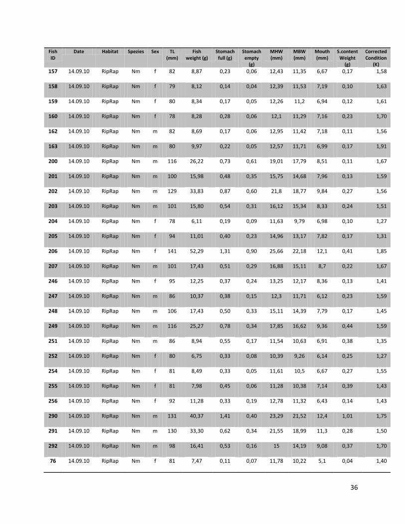
36
Fish ID
Date Habitat Spezies Sex TL (mm)
Fish weight (g)
Stomach full (g)
Stomach empty
(g)
MHW (mm)
MBW (mm)
Mouth (mm)
S.content Weight
(g)
Corrected Condition
(K)
157 14.09.10 RipRap Nm f 82 8,87 0,23 0,06 12,43 11,35 6,67 0,17 1,58
158 14.09.10 RipRap Nm f 79 8,12 0,14 0,04 12,39 11,53 7,19 0,10 1,63
159 14.09.10 RipRap Nm f 80 8,34 0,17 0,05 12,26 11,2 6,94 0,12 1,61
160 14.09.10 RipRap Nm f 78 8,28 0,28 0,06 12,1 11,29 7,16 0,23 1,70
162 14.09.10 RipRap Nm m 82 8,69 0,17 0,06 12,95 11,42 7,18 0,11 1,56
163 14.09.10 RipRap Nm m 80 9,97 0,22 0,05 12,57 11,71 6,99 0,17 1,91
200 14.09.10 RipRap Nm m 116 26,22 0,73 0,61 19,01 17,79 8,51 0,11 1,67
201 14.09.10 RipRap Nm m 100 15,98 0,48 0,35 15,75 14,68 7,96 0,13 1,59
202 14.09.10 RipRap Nm m 129 33,83 0,87 0,60 21,8 18,77 9,84 0,27 1,56
203 14.09.10 RipRap Nm m 101 15,80 0,54 0,31 16,12 15,34 8,33 0,24 1,51
204 14.09.10 RipRap Nm f 78 6,11 0,19 0,09 11,63 9,79 6,98 0,10 1,27
205 14.09.10 RipRap Nm f 94 11,01 0,40 0,23 14,96 13,17 7,82 0,17 1,31
206 14.09.10 RipRap Nm f 141 52,29 1,31 0,90 25,66 22,18 12,1 0,41 1,85
207 14.09.10 RipRap Nm m 101 17,43 0,51 0,29 16,88 15,11 8,7 0,22 1,67
246 14.09.10 RipRap Nm f 95 12,25 0,37 0,24 13,25 12,17 8,36 0,13 1,41
247 14.09.10 RipRap Nm m 86 10,37 0,38 0,15 12,3 11,71 6,12 0,23 1,59
248 14.09.10 RipRap Nm m 106 17,43 0,50 0,33 15,11 14,39 7,79 0,17 1,45
249 14.09.10 RipRap Nm m 116 25,27 0,78 0,34 17,85 16,62 9,36 0,44 1,59
251 14.09.10 RipRap Nm m 86 8,94 0,55 0,17 11,54 10,63 6,91 0,38 1,35
252 14.09.10 RipRap Nm f 80 6,75 0,33 0,08 10,39 9,26 6,14 0,25 1,27
254 14.09.10 RipRap Nm f 81 8,49 0,33 0,05 11,61 10,5 6,67 0,27 1,55
255 14.09.10 RipRap Nm f 81 7,98 0,45 0,06 11,28 10,38 7,14 0,39 1,43
256 14.09.10 RipRap Nm f 92 11,28 0,33 0,19 12,78 11,32 6,43 0,14 1,43
290 14.09.10 RipRap Nm m 131 40,37 1,41 0,40 23,29 21,52 12,4 1,01 1,75
291 14.09.10 RipRap Nm m 130 33,30 0,62 0,34 21,55 18,99 11,3 0,28 1,50
292 14.09.10 RipRap Nm m 98 16,41 0,53 0,16 15 14,19 9,08 0,37 1,70
76 14.09.10 RipRap Nm f 81 7,47 0,11 0,07 11,78 10,22 5,1 0,04 1,40

37
Fish ID
Date Habitat Spezies Sex TL (mm)
Fish weight (g)
Stomach full (g)
Stomach empty
(g)
MHW (mm)
MBW (mm)
Mouth (mm)
S.content Weight
(g)
Corrected Condition
(K)
78 14.09.10 RipRap Nm f 98 13,69 0,45 0,19 14,68 13,96 5,92 0,26 1,43
79 14.09.10 RipRap Nm m 100 15,25 0,49 0,18 15,41 14,24 5,34 0,32 1,49
80 14.09.10 RipRap Nm f 85 9,95 0,37 0,17 14,43 12,92 4,62 0,20 1,59
81 14.09.10 RipRap Nm f 86 9,42 0,42 0,10 13,39 11,97 5,59 0,32 1,43
82 14.09.10 RipRap Nm f 77 6,58 0,14 0,05 11,92 10,02 4,81 0,09 1,42
83 14.09.10 RipRap Nm m 120 30,44 0,90 0,38 21,98 20,68 8,79 0,51 1,73
86 14.09.10 RipRap Nm m 70 4,99 0,10 0,02 10,07 7,97 4,14 0,08 1,43
128 14.09.10 RipRap Nm f 115 23,91 1,08 0,54 18,24 15,83 9,02 0,54 1,54
130 14.09.10 RipRap Nm m 77 6,17 0,20 0,12 10,63 10,18 6,24 0,07 1,34
14 14.09.10 RipRap Pk f 84 7,22 0,25 0,20 14,04 13,46 5,23 0,05 1,21
18 14.09.10 RipRap Pk f 102 15,70 0,67 0,41 18,48 17,35 6,69 0,26 1,45
21 14.09.10 RipRap Pk m 114 18,38 0,48 0,38 19,06 19,07 6,54 0,09 1,23
25 14.09.10 RipRap Pk m 106 17,54 0,63 0,25 21,98 17,31 7,83 0,39 1,44
40 14.09.10 RipRap Pk m 79 6,44 0,35 0,17 13,36 11,33 5,88 0,18 1,27
42 14.09.10 RipRap Pk m 121 28,30 0,94 0,83 23,71 20,8 8,81 0,10 1,59
49 14.09.10 RipRap Pk f 116 20,99 0,56 0,27 21,47 19,7 7,94 0,29 1,33
51 14.09.10 RipRap Pk f 111 19,12 0,64 0,46 20,34 18,99 7,52 0,17 1,39
52 14.09.10 RipRap Pk f 107 16,76 0,65 0,41 18,89 17,69 7,79 0,25 1,35
61 14.09.10 RipRap Pk f 116 23,95 1,10 0,48 23 20,74 7,44 0,62 1,49
63 14.09.10 RipRap Pk m 111 21,45 0,87 0,39 20,58 19,9 6,88 0,48 1,53
64 14.09.10 RipRap Pk f 119 23,14 0,58 0,39 21,66 18,74 7,15 0,19 1,36
66 14.09.10 RipRap Pk m 123 26,80 1,07 0,51 22,27 20,95 7,99 0,56 1,41
67 14.09.10 RipRap Pk f 130 32,17 0,96 0,69 25,77 23,28 8,54 0,28 1,45
68 14.09.10 RipRap Pk f 121 25,89 0,78 0,56 29,02 20,88 8,52 0,22 1,45
77 14.09.10 RipRap Pk m 133 34,03 1,20 0,75 23,56 21,59 8,81 0,45 1,43
84 14.09.10 RipRap Pk f 110 18,13 0,51 0,31 18,53 17,62 7,28 0,21 1,35
85 14.09.10 RipRap Pk m 65 3,41 0,05 0,02 9,72 8,04 4,36 0,03 1,23

38
Fish ID
Date Habitat Spezies Sex TL (mm)
Fish weight (g)
Stomach full (g)
Stomach empty
(g)
MHW (mm)
MBW (mm)
Mouth (mm)
S.content Weight
(g)
Corrected Condition
(K)
87 14.09.10 RipRap Pk m 78 5,80 0,26 0,08 11,74 9,65 5,41 0,18 1,18
88 14.09.10 RipRap Pk m 67 3,80 0,07 0,02 10,02 8,33 4,87 0,05 1,25
120 14.09.10 RipRap Pk f 100 16,64 0,58 0,33 19,56 17,11 8,77 0,26 1,64
129 14.09.10 RipRap Pk m 72 4,79 0,21 0,16 11,78 10,16 6,82 0,05 1,27
131 14.09.10 RipRap Pk m 126 30,71 1,28 0,91 29,12 18,73 10,8 0,37 1,52
134 14.09.10 RipRap Pk f 60 2,46 0,08 0,02 9,19 6,74 5,44 0,06 1,11
142 14.09.10 RipRap Pk f 79 7,02 0,28 0,14 11,79 10,76 6,95 0,14 1,40
147 14.09.10 RipRap Pk f 144 44,74 1,86 1,18 27,02 25,86 10,7 0,68 1,48
149 14.09.10 RipRap Pk m 124 27,96 1,41 0,53 22,46 20,85 10,1 0,88 1,42
153 14.09.10 RipRap Pk m 76 5,84 0,16 0,07 11,56 10,51 5,61 0,09 1,31
156 14.09.10 RipRap Pk f 84 8,23 0,24 0,14 13,16 12,08 7,48 0,10 1,37
161 14.09.10 RipRap Pk f 77 6,48 0,22 0,11 12,72 11,24 6,95 0,11 1,40
250 14.09.10 RipRap Pk f 68 3,87 0,18 0,11 9,83 7,56 6,22 0,07 1,21
253 14.09.10 RipRap Pk f 120 24,05 0,98 0,45 19,71 17,89 11 0,53 1,36
285 14.09.10 RipRap Pk f 112 21,73 0,91 0,30 21,45 17,46 9,11 0,61 1,50
1 14.09.10 Sand Nm m 92 13,07 0,44 0,23 15,62 14,98 6,32 0,21 1,65
2 14.09.10 Sand Nm m 107 20,34 0,65 0,49 18,27 16,39 7,29 0,16 1,65
3 14.09.10 Sand Nm f 94 12,53 0,42 0,31 15,32 14,04 6,09 0,11 1,50
4 14.09.10 Sand Nm m 92 12,31 0,48 0,18 15,39 14 5,64 0,30 1,54
5 14.09.10 Sand Nm f 97 15,24 0,54 0,39 16,24 15,12 7,34 0,15 1,65
6 14.09.10 Sand Nm f 88 9,78 0,58 0,16 14,91 13,18 5,31 0,41 1,37
7 14.09.10 Sand Nm m 110 20,19 0,90 0,41 18,56 17,51 7,55 0,49 1,48
8 14.09.10 Sand Nm f 87 9,51 0,39 0,13 14,18 13,6 4,84 0,26 1,40
9 14.09.10 Sand Nm m 94 12,73 0,43 0,37 15,66 14,84 5,96 0,06 1,53
11 14.09.10 Sand Nm f 85 9,61 0,29 0,17 12,54 11,92 4,68 0,12 1,55
12 14.09.10 Sand Nm f 83 8,93 0,21 0,17 13,44 11,73 4,76 0,04 1,55
13 14.09.10 Sand Nm f 88 9,86 0,32 0,18 14,01 13,18 5,36 0,13 1,43

39
Fish ID
Date Habitat Spezies Sex TL (mm)
Fish weight (g)
Stomach full (g)
Stomach empty
(g)
MHW (mm)
MBW (mm)
Mouth (mm)
S.content Weight
(g)
Corrected Condition
(K)
15 14.09.10 Sand Nm m 87 9,13 0,29 0,15 13,81 13,21 5,59 0,14 1,37
16 14.09.10 Sand Nm m 134 48,37 1,42 1,02 25,53 23,79 7,46 0,40 1,99
17 14.09.10 Sand Nm m 111 21,51 0,53 0,51 17,82 17,24 6,96 0,02 1,57
19 14.09.10 Sand Nm f 95 14,80 0,50 0,42 16,19 15,84 5,74 0,08 1,72
20 14.09.10 Sand Nm m 96 13,57 0,62 0,35 16,91 15,77 6,71 0,27 1,50
22 14.09.10 Sand Nm f 87 11,13 0,51 0,43 14,1 12,39 5,41 0,08 1,68
23 14.09.10 Sand Nm m 98 15,11 0,53 0,34 15,78 15,42 6,99 0,19 1,59
24 14.09.10 Sand Nm f 84 8,30 0,33 0,15 11,53 10,68 6,2 0,19 1,37
28 14.09.10 Sand Nm f 106 19,12 0,52 0,38 16,88 16,03 7,3 0,14 1,59
29 14.09.10 Sand Nm m 116 26,22 0,77 0,56 19,3 18,57 7,77 0,21 1,67
30 14.09.10 Sand Nm m 95 13,31 0,28 0,18 15,18 14,46 5,99 0,10 1,54
31 14.09.10 Sand Nm f 87 11,31 0,29 0,15 14,58 13,66 5,47 0,14 1,70
32 14.09.10 Sand Nm m 96 12,69 0,39 0,25 15,55 14,16 5,87 0,14 1,42
33 14.09.10 Sand Nm f 89 11,00 0,41 0,16 15,51 15,24 4,73 0,25 1,52
34 14.09.10 Sand Nm f 85 9,90 0,34 0,13 14,52 13,58 5,57 0,21 1,58
35 14.09.10 Sand Nm f 80 7,97 0,21 0,14 11,75 11,09 5,43 0,07 1,54
36 14.09.10 Sand Nm f 83 8,05 0,26 0,13 12,26 11,86 5,56 0,13 1,39
37 14.09.10 Sand Nm m 90 11,92 0,45 0,28 15,92 15,24 5,65 0,16 1,61
38 14.09.10 Sand Nm f 90 11,68 0,38 0,20 15,44 14,92 5,84 0,18 1,58
39 14.09.10 Sand Nm m 89 10,08 0,22 0,10 13,98 13,14 5,77 0,12 1,41
164 14.09.10 Sand Nm m 103 17,92 0,76 0,35 15,67 13,74 8,13 0,41 1,60
165 14.09.10 Sand Nm m 91 11,54 0,30 0,23 13,92 12,71 7,59 0,08 1,52
166 14.09.10 Sand Nm f 73 6,38 0,19 0,13 11,14 10,06 6,97 0,06 1,62
167 14.09.10 Sand Nm f 91 13,01 0,65 0,32 14,11 12,88 8,44 0,32 1,68
168 14.09.10 Sand Nm f 94 14,35 0,44 0,29 15,77 14,31 8,62 0,15 1,71
169 14.09.10 Sand Nm f 88 10,15 0,60 0,24 13,43 11,89 6,24 0,36 1,44
170 14.09.10 Sand Nm f 95 13,81 0,30 0,23 14,81 13,65 7,95 0,07 1,60

40
Fish ID
Date Habitat Spezies Sex TL (mm)
Fish weight (g)
Stomach full (g)
Stomach empty
(g)
MHW (mm)
MBW (mm)
Mouth (mm)
S.content Weight
(g)
Corrected Condition
(K)
171 14.09.10 Sand Nm f 79 9,08 0,20 0,14 12,59 11,67 7,99 0,06 1,83
172 14.09.10 Sand Nm f 101 16,41 0,39 0,18 16,53 15,22 8,49 0,21 1,57
173 14.09.10 Sand Nm m 79 7,58 0,24 0,05 12,02 10,93 6,71 0,19 1,50
174 14.09.10 Sand Nm f 81 9,16 0,23 0,06 11,84 10,92 7,32 0,17 1,69
175 14.09.10 Sand Nm m 91 11,99 0,41 0,23 13,58 11,93 7,93 0,19 1,57
176 14.09.10 Sand Nm f 84 10,46 0,24 0,13 14,01 13,17 7,13 0,10 1,75
177 14.09.10 Sand Nm f 91 12,52 0,31 0,11 14,46 12,39 7,38 0,20 1,63
178 14.09.10 Sand Nm m 82 9,41 0,17 0,06 11,93 11,02 7,54 0,11 1,69
179 14.09.10 Sand Nm f 81 9,23 0,11 0,07 11,01 10,09 7,03 0,04 1,73
180 14.09.10 Sand Nm m 109 20,61 0,68 0,46 16,12 14,77 9,07 0,22 1,57
182 14.09.10 Sand Nm m 67 4,53 0,13 0,08 8,56 7,55 6,49 0,05 1,49
183 14.09.10 Sand Nm f 105 18,03 1,04 0,51 16,27 15,02 7,65 0,53 1,51
184 14.09.10 Sand Nm m 127 33,19 0,71 0,62 21,28 19,38 11,1 0,09 1,62
185 14.09.10 Sand Nm f 92 12,44 0,31 0,13 14,77 13,21 8,77 0,18 1,57
186 14.09.10 Sand Nm f 99 17,05 0,58 0,31 16,04 14,79 7,54 0,28 1,73
187 14.09.10 Sand Nm f 85 10,05 0,35 0,19 14,09 13,17 7,11 0,16 1,61
188 14.09.10 Sand Nm m 82 8,02 0,25 0,06 12 10,86 6,44 0,19 1,42
189 14.09.10 Sand Nm m 103 17,91 0,79 0,37 16,87 15,69 9,16 0,42 1,60
190 14.09.10 Sand Nm f 87 10,87 0,35 0,21 12,57 11,34 8,32 0,14 1,63
191 14.09.10 Sand Nm m 104 18,66 0,54 0,24 16,06 15,23 9,49 0,31 1,63
192 14.09.10 Sand Nm f 81 8,98 0,30 0,07 11,24 10,65 7,05 0,23 1,65
193 14.09.10 Sand Nm f 98 16,14 0,39 0,17 16,4 14,97 8,52 0,22 1,69
194 14.09.10 Sand Nm f 92 12,77 0,58 0,32 14,86 12,69 7,48 0,27 1,61
195 14.09.10 Sand Nm m 90 11,98 0,40 0,15 13,28 11,73 7,87 0,25 1,61
282 14.09.10 Sand Nm m 119 27,75 0,68 0,32 18,5 17,77 10,3 0,36 1,63
284 14.09.10 Sand Nm m 126 35,36 0,95 0,44 21,94 20,39 10,1 0,51 1,74
286 14.09.10 Sand Nm m 101 17,12 0,50 0,16 16,12 15,37 8,07 0,34 1,63

41
Fish ID
Date Habitat Spezies Sex TL (mm)
Fish weight (g)
Stomach full (g)
Stomach empty
(g)
MHW (mm)
MBW (mm)
Mouth (mm)
S.content Weight
(g)
Corrected Condition
(K)
287 14.09.10 Sand Nm m 100 15,21 0,52 0,18 15,63 14,01 7,92 0,34 1,49
288 14.09.10 Sand Nm m 92 12,90 0,45 0,18 14,96 14,01 8,02 0,27 1,62
Tab. C: Raw data of the two species N. melanostomus (Nm) and P. kessleri (Pk) caught in two different habitats (sand; riprap) in the Lower Rhine, Germany on the 5th July 2011
Fish ID
Date Habitat Spezies Sex TL (mm)
Fish weight
(g)
Stomach full (g)
Stomach empty
(g)
MHW (mm)
MBW (mm)
Mouth (mm)
S.content Weight
(g)
Corrected Condition
(K)
208 5.07.11 Riprap Nm m 107 20,60 0,99 0,60 17,62 15,29 10,4 0,39 1,65
209 5.07.11 Riprap Nm m 102 17,14 1,28 0,34 16,41 15,14 8,78 0,94 1,53
210 5.07.11 Riprap Nm f 73 5,81 0,34 0,22 9,61 8,32 6,64 0,12 1,46
211 5.07.11 Riprap Nm f 100 17,45 0,61 0,19 15,21 14,11 9,85 0,42 1,70
212 5.07.11 Riprap Nm m 90 10,93 0,63 0,11 11,42 10,38 7,81 0,52 1,43
213 5.07.11 Riprap Nm m 77 6,38 0,15 0,09 9,58 8,75 5,25 0,06 1,38
214 5.07.11 Riprap Nm m 95 12,48 0,85 0,20 12,61 11,53 6,94 0,65 1,38
215 5.07.11 Riprap Nm f 78 6,47 0,23 0,12 10,27 9,2 5,26 0,11 1,34
216 5.07.11 Riprap Nm f 81 8,18 0,45 0,09 10,78 9,59 6,47 0,36 1,47
218 5.07.11 Riprap Nm m 112 22,96 0,36 0,26 17,65 16,32 10,3 0,10 1,63
219 5.07.11 Riprap Nm f 70 5,76 0,27 0,07 9,38 8,41 6,65 0,20 1,62
220 5.07.11 Riprap Nm m 71 5,09 0,36 0,08 8,79 7,77 5,67 0,28 1,34
221 5.07.11 Riprap Nm f 65 4,20 0,07 0,04 8,51 7,6 5,21 0,04 1,51
222 5.07.11 Riprap Nm f 68 4,70 0,17 0,05 9,1 7,97 5,63 0,11 1,46
223 5.07.11 Riprap Nm f 65 3,79 0,20 0,06 8,42 7,37 5,36 0,14 1,33
224 5.07.11 Riprap Nm m 92 10,42 0,39 0,14 11,79 10,83 6,72 0,25 1,31
225 5.07.11 Riprap Nm f 101 17,29 1,12 0,30 15,65 14,27 7,68 0,82 1,60
226 5.07.11 Riprap Nm m 101 15,28 0,89 0,21 15,27 13,98 7,91 0,68 1,42
227 5.07.11 Riprap Nm f 85 8,77 0,37 0,11 11,53 10,17 6,02 0,27 1,38
228 5.07.11 Riprap Nm m 109 20,15 0,67 0,28 16,79 15,03 9,81 0,39 1,53
229 5.07.11 Riprap Nm f 67 3,47 0,06 0,05 8,43 7,13 5,11 0,01 1,15
230 5.07.11 Riprap Nm f 79 7,28 0,25 0,16 11,05 9,79 6,66 0,10 1,46
231 5.07.11 Riprap Nm m 70 5,18 0,17 0,07 8,57 7,79 6,13 0,10 1,48
257 5.07.11 Riprap Nm m 119 28,89 0,65 0,43 17,76 16,46 10,7 0,22 1,70
258 5.07.11 Riprap Nm m 92 12,89 0,62 0,20 13,21 11,84 7,37 0,42 1,60
259 5.07.11 Riprap Nm f 69 4,51 0,28 0,06 8,32 7,07 4,78 0,21 1,31
260 5.07.11 Riprap Nm f 106 20,07 0,93 0,49 17,14 16,04 9,53 0,44 1,65
261 5.07.11 Riprap Nm m 118 27,99 1,25 0,48 18,81 17,32 8,84 0,76 1,66
262 5.07.11 Riprap Nm m 98 13,49 0,72 0,26 14,06 13,34 7,29 0,46 1,38
263 5.07.11 Riprap Nm m 88 9,59 0,42 0,12 11,51 10,48 6,58 0,30 1,36
264 5.07.11 Riprap Nm m 96 13,57 0,42 0,20 14,35 13,19 9,74 0,22 1,51
265 5.07.11 Riprap Nm m 81 8,19 0,42 0,14 11,24 10,4 6,11 0,28 1,49
266 5.07.11 Riprap Nm f 75 7,35 0,26 0,08 10,24 9,6 6,55 0,17 1,70

42
Fish ID
Date Habitat Spezies Sex TL (mm)
Fish weight
(g)
Stomach full (g)
Stomach empty
(g)
MHW (mm)
MBW (mm)
Mouth (mm)
S.content Weight
(g)
Corrected Condition
(K)
278 5.07.11 Riprap Nm f 107 18,01 0,85 0,35 16,73 15,35 8,28 0,50 1,43
279 5.07.11 Riprap Nm f 75 6,74 0,22 0,09 10,3 9,33 6,28 0,13 1,57
280 5.07.11 Riprap Nm m 90 10,73 0,52 0,19 12,96 11,77 8,01 0,32 1,43
281 5.07.11 Riprap Nm m 78 7,03 0,31 0,15 11,08 9,73 5,81 0,16 1,45
271 5.07.11 Riprap Pk f 66 5,09 0,13 0,05 8,89 7,94 6,41 0,08 1,74
232 5.07.11 Sand Nm m 91 11,56 0,46 0,33 13,18 12,46 7,26 0,13 1,52
233 5.07.11 Sand Nm m 99 15,98 0,88 0,34 16,19 14,79 8,41 0,54 1,59
234 5.07.11 Sand Nm f 78 7,87 0,35 0,17 10,89 9,96 5,43 0,18 1,62
235 5.07.11 Sand Nm f 71 6,09 0,22 0,12 9,84 9,14 5,11 0,10 1,67
236 5.07.11 Sand Nm m 90 12,23 0,56 0,21 13,06 12,41 6,83 0,35 1,63
237 5.07.11 Sand Nm f 74 6,02 0,18 0,09 9,58 8,62 5,3 0,08 1,47
238 5.07.11 Sand Nm f 97 15,79 0,63 0,20 14,96 13,9 8,34 0,43 1,68
239 5.07.11 Sand Nm f 80 7,48 0,24 0,05 10,85 9,51 5,32 0,19 1,42
240 5.07.11 Sand Nm f 84 10,38 0,43 0,27 12,88 11,61 7,51 0,16 1,72
241 5.07.11 Sand Nm m 88 10,75 0,26 0,10 13,54 12,35 7,57 0,16 1,55
242 5.07.11 Sand Nm m 92 12,35 0,49 0,32 13,39 12,69 7,58 0,18 1,56
243 5.07.11 Sand Nm m 90 11,54 0,33 0,20 13 12,12 7,44 0,13 1,57
244 5.07.11 Sand Nm m 86 9,55 0,38 0,18 11,87 10,91 6,66 0,20 1,47
245 5.07.11 Sand Nm m 100 17,61 0,47 0,21 15,28 13,91 9,21 0,26 1,74
268 5.07.11 Sand Nm f 108 20,76 0,77 0,42 16,98 15,75 9 0,36 1,62
269 5.07.11 Sand Nm m 90 11,31 0,43 0,21 12,66 11,44 7,27 0,22 1,52
270 5.07.11 Sand Nm f 118 22,89 1,01 0,47 17,41 16,22 10,3 0,54 1,36
272 5.07.11 Sand Nm f 99 14,10 0,50 0,25 14,06 12,83 8,03 0,25 1,43
273 5.07.11 Sand Nm m 79 8,04 0,41 0,16 10,79 9,98 6,86 0,25 1,58
274 5.07.11 Sand Nm m 81 9,28 0,36 0,16 11,57 10,61 7,62 0,20 1,71
275 5.07.11 Sand Nm m 79 7,60 0,28 0,13 11,08 10,41 5,61 0,15 1,51
277 5.07.11 Sand Nm f 66 4,45 0,16 0,05 8,71 7,53 5,29 0,11 1,51

43
Appendix 3 Regression analysis of habitat RipRap
(statistical calculations created in SPSS)
Raw data for comparision between linear and quadratic regression
FOR Number 1 (according Tab. 3)
Linear

44
For Number 2 (according Tab. 3)
Linear
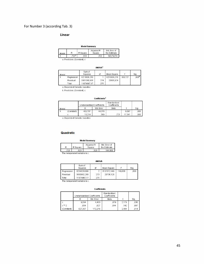
45
For Number 3 (according Tab. 3)
Linear
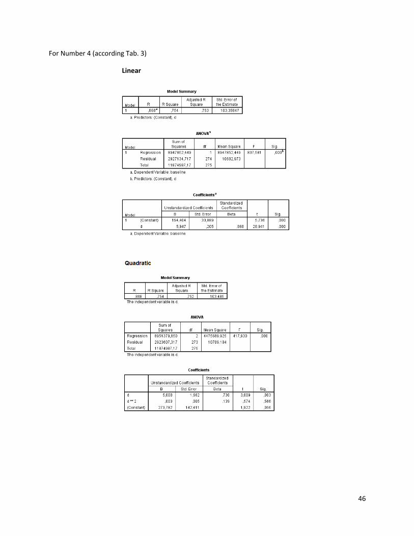
46
For Number 4 (according Tab. 3)
Linear

47
For Number 5 (according Tab. 3)
Linear
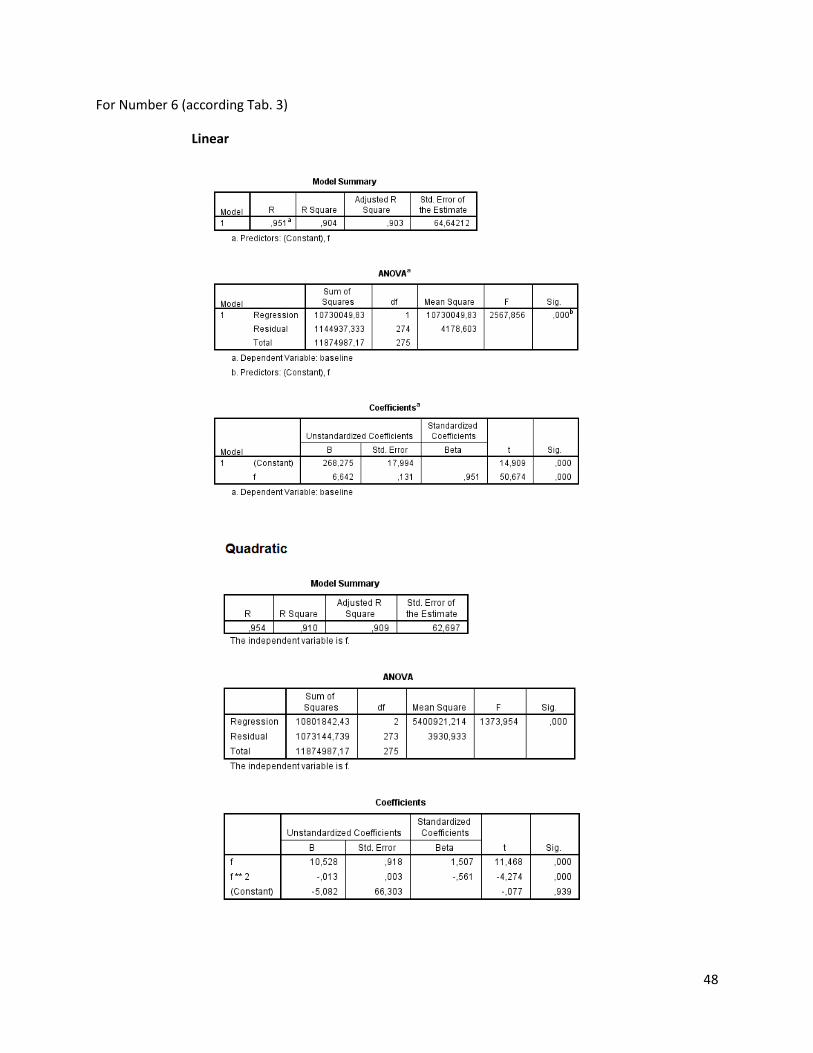
48
For Number 6 (according Tab. 3)
Linear
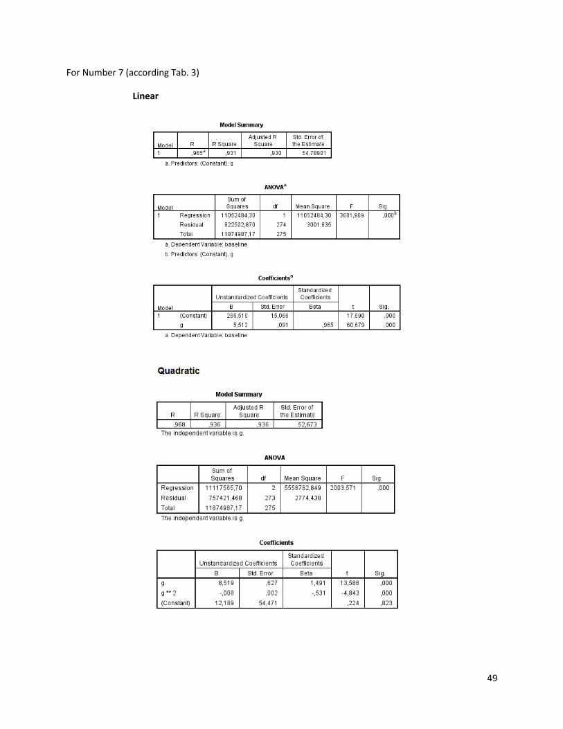
49
For Number 7 (according Tab. 3)
Linear

50
For Number 8 (according Tab. 3)
Linear
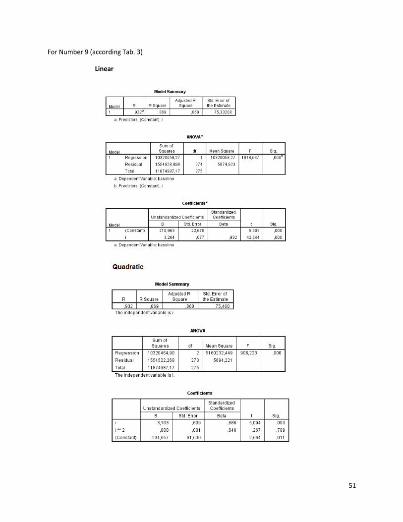
51
For Number 9 (according Tab. 3)
Linear

52
For Number 10 (according Tab. 3)
Linear
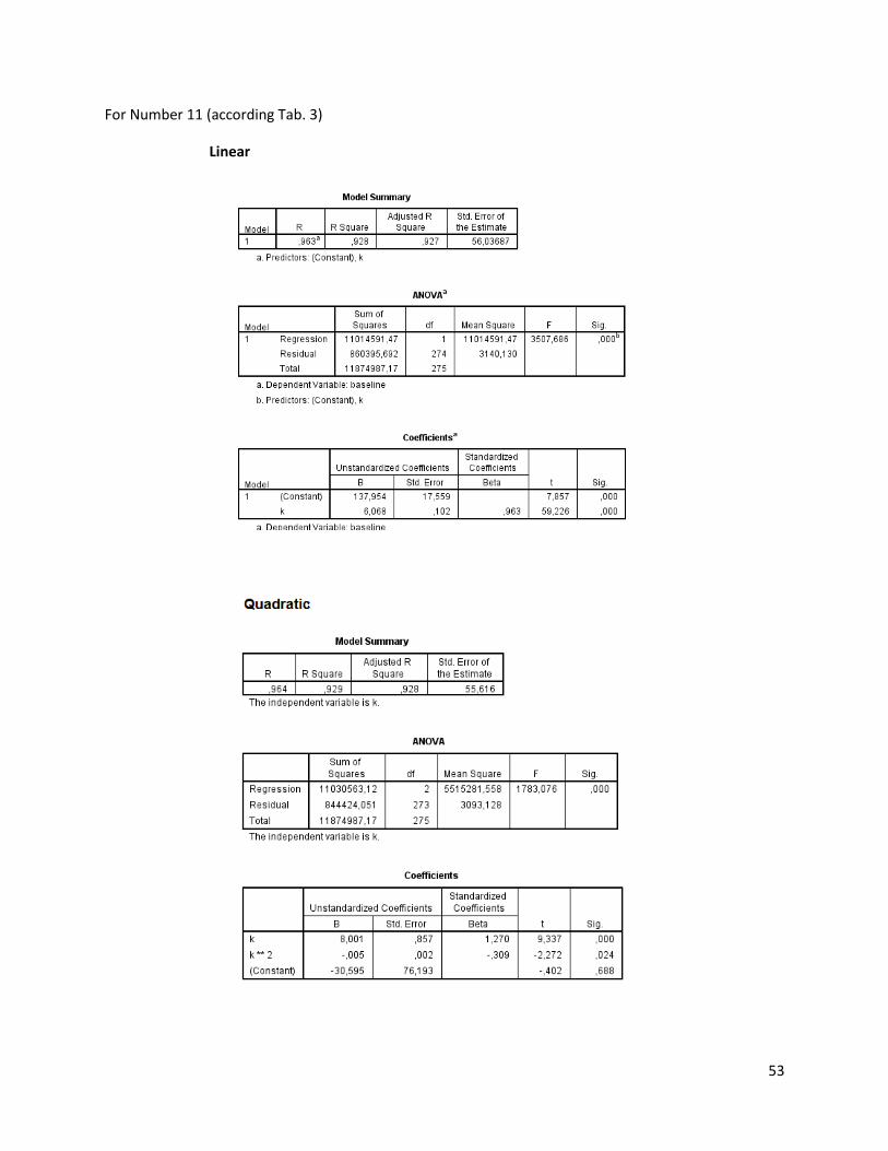
53
For Number 11 (according Tab. 3)
Linear
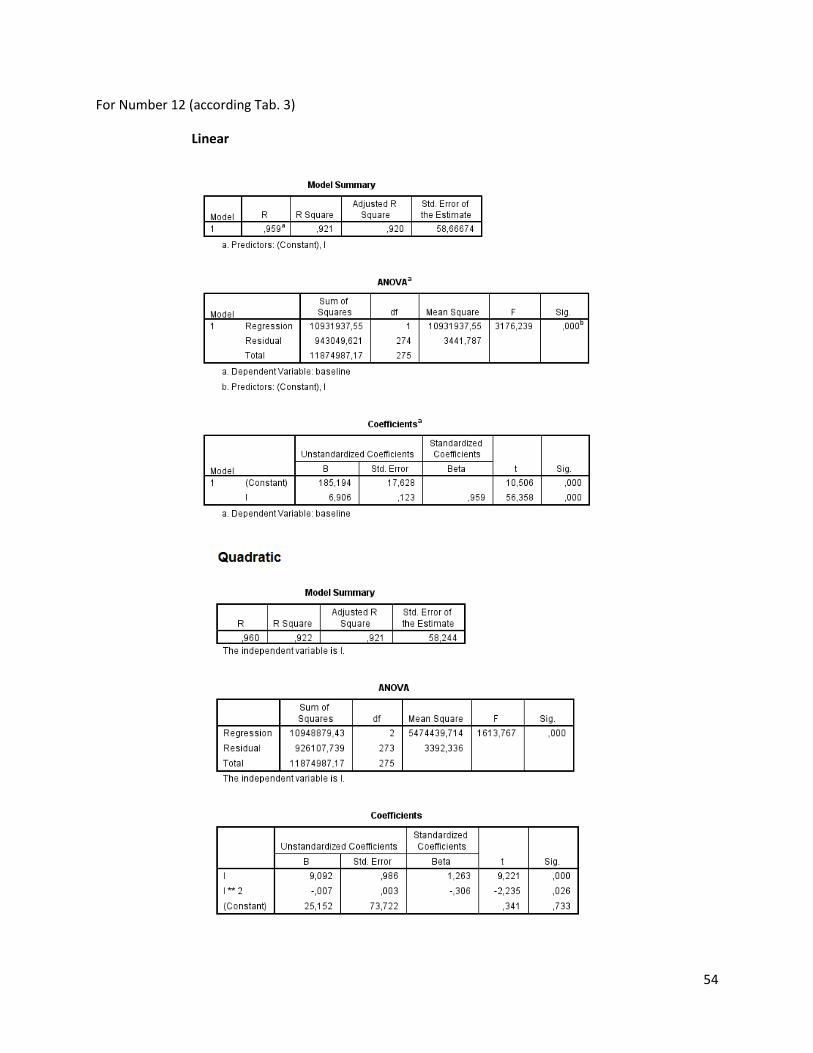
54
For Number 12 (according Tab. 3)
Linear

55
For Number 13 (according Tab. 3)
Linear

56
For Number 14 (according Tab. 3)
Linear

57
For Number 15 (according Tab. 3)
Linear
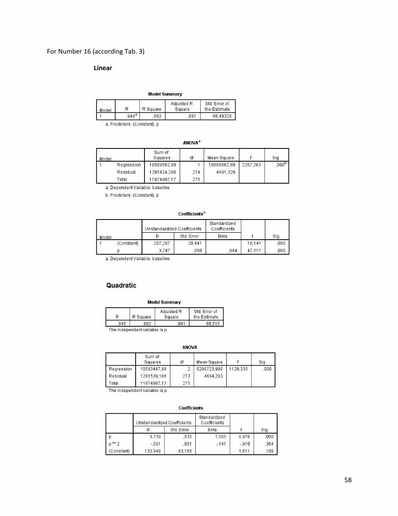
58
For Number 16 (according Tab. 3)
Linear
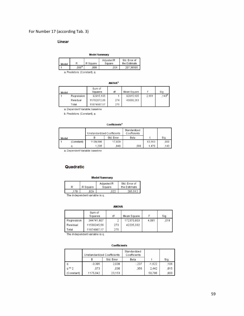
59
For Number 17 (according Tab. 3)
Linear
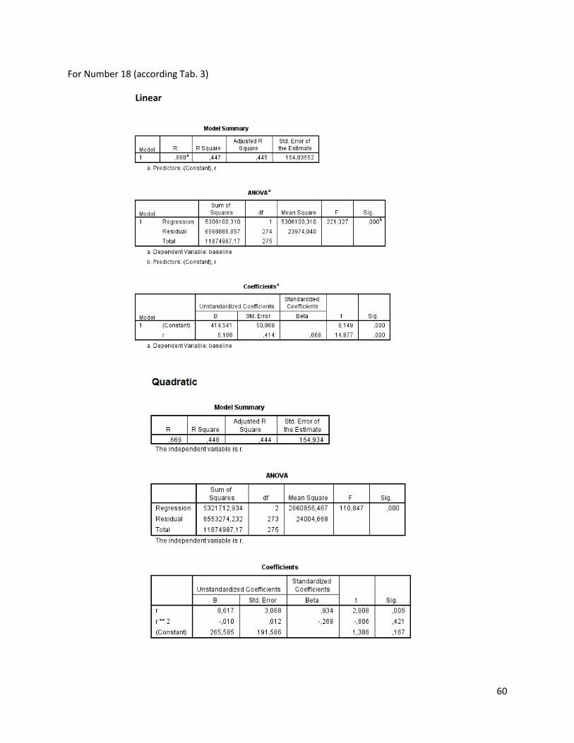
60
For Number 18 (according Tab. 3)
Linear
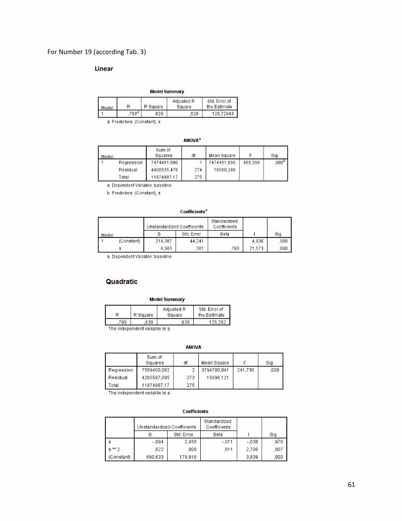
61
For Number 19 (according Tab. 3)
Linear

62
For Number 20 (according Tab. 3)
Linear

63
For Number 21 (according Tab. 3)
Linear

64
For Number 22 (according Tab. 3)
Linear

65
For Number 23 (according Tab. 3)
Linear
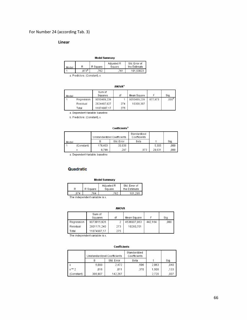
66
For Number 24 (according Tab. 3)
Linear
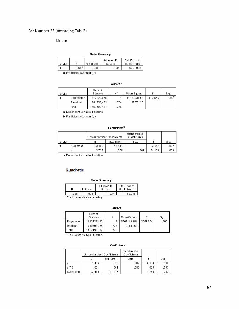
67
For Number 25 (according Tab. 3)
Linear

68
For Number 26 (according Tab. 3)
Linear
69
For Number 27 (according Tab. 3)
Linear

70
For Number 28 (according Tab. 3)
Linear

71
For Number 29 (according Tab. 3)
Linear

72
For Number 30 (according Tab. 3)
Linear

73
For Number 31 (according Tab. 3)
Linear

74
For Number 32 (according Tab. 3)
Linear

75
Appendix 4: Regression analysis N. melanostomus (sand) Tab. D: Regression analysis of 33 different measuring variables (calculated with TmorphGen6b) for N.melanostomus (sand) plotted against standard length (SL). Correlation coefficient for linear regression (R2L) and quadratic regression (R2Q), n=103.
Number (Fig.2)
Measured variable R2L R2Q F-test Q/L P Best explanation
2 Mouthdepth 0.589 0.593 4.68 ns - 3 Mouth end -VF 0.871 0.872 3.97 ns - 4 Eye –highest spot Po 0.517 0.518 0,92 ns - 5 Eye –highest spot Op 0.755 0.755 0 ns - 6 Highest spot Po – highest
spot Op 0.583 0.588 5.80 <0.05 Q
7 Eye – mouthend 0.904 0.909 28.76 <0.01 Q 8 Hight Po 0.931 0.937 43.14 <0.01 Q 9 Contact spot VF 0.945 0.945 0 ns -
10 Begin 1D - VF 0.869 0.869 0 ns - 11 Begin 2D – begin AF 0.913 0.916 17.13 <0.01 Q 12 End 2D – end AF 0.928 0.929 6.01 <0.05 Q 13 Contact point VerF 0.923 0.924 5.83 <0.05 Q 14 Contact point PF 0.495 0.495 0 ns - 15 Length 1D 0.816 0.818 5.17 <0.05 Q 16 Length 2D 0.944 0.945 8.11 <0.05 Q 17 Length AF 0.890 0.890 0 ns - 18 End 1D – begin 2D 0.010 0.023 6.40 <0.05 Q
19 End 2D – dorsal contact point VerF
0.450 0.446 3.48 ns -
20 End AF – ventral contact point VerF
0.629 0.639 13.61 <0.01 Q
21 VF – begin AF 0.830 0.833 8.19 <0.05 Q
22 Dorsal contact point VerF - MVerF
0.888 0.889 4.23 ns -
23 Ventral contact point VerF - MVerF
0.881 0.883 8.26 <0.05 Q
24 VF – contact point Po/Op 0.804 0.804 0 ns -
25 Upper lip - eye 0.762 0.764 3.89 ns -
26 Eye – begin 1D 0.940 0.940 0 ns -
27 Upper lip – 1D 0.949 0.949 0 ns -
28 Upper lip – dorsal contact point PF
0.886 0.886 0 ns -
29 Upper lip – ventral contact point PF
0.832 0.832 0 ns -

76
30 Mouth end – contact point Po/Op
0.666 0.667 1.42 ns -
31 Begin 2D - VF 0.892 0.893 4.88 ns -
32 End 2D -VF 0.966 0.966 0 ns -
33 Begin 1D – end AF 0.981 0.981 0 ns -
34 Begin 1D – begin AF 0.947 0.948 10.54 <0.01 Q
The following abbreviations are used: ns (not significant), 1D (first dorsal fin), 2D (second dorsal fin), AF (anal fin), MVerF (middle of vertical
fin), Op (Operculum), PF (Pectoral fin), Po (Praeoperculum), VerF (vertical fin), VF (ventral fin).
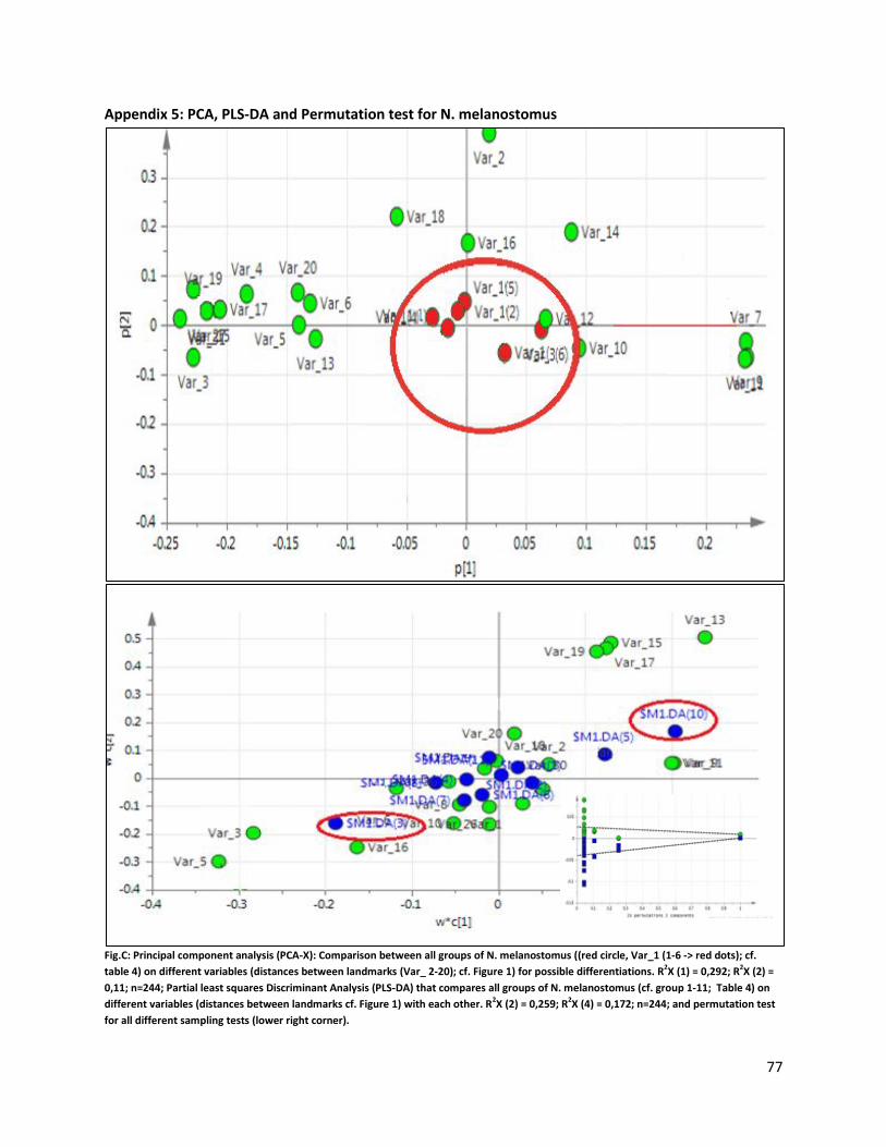
77
Appendix 5: PCA, PLS-DA and Permutation test for N. melanostomus
Fig.C: Principal component analysis (PCA-X): Comparison between all groups of N. melanostomus ((red circle, Var_1 (1-6 -> red dots); cf.
table 4) on different variables (distances between landmarks (Var_ 2-20); cf. Figure 1) for possible differentiations. R2X (1) = 0,292; R2X (2) =
0,11; n=244; Partial least squares Discriminant Analysis (PLS-DA) that compares all groups of N. melanostomus (cf. group 1-11; Table 4) on
different variables (distances between landmarks cf. Figure 1) with each other. R2X (2) = 0,259; R2X (4) = 0,172; n=244; and permutation test
for all different sampling tests (lower right corner).
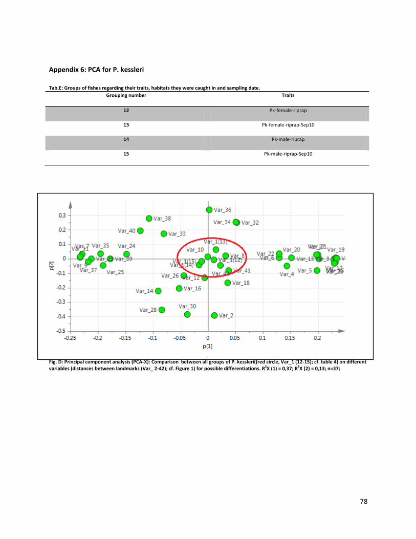
78
Appendix 6: PCA for P. kessleri
Tab.E: Groups of fishes regarding their traits, habitats they were caught in and sampling date.
Grouping number Traits
12 Pk-female-riprap
13 Pk-female-riprap-Sep10
14 Pk-male-riprap
15 Pk-male-riprap-Sep10
Fig. D: Principal component analysis (PCA-X): Comparison between all groups of P. kessleri((red circle, Var_1 (12-15); cf. table 4) on different variables (distances between landmarks (Var_ 2-42); cf. Figure 1) for possible differentiations. R2X (1) = 0,37; R2X (2) = 0,13; n=37;
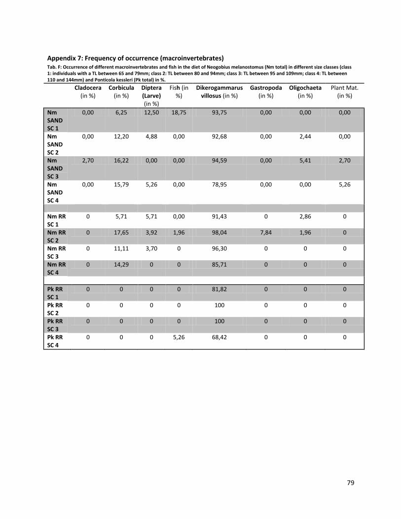
79
Appendix 7: Frequency of occurrence (macroinvertebrates) Tab. F: Occurrence of different macroinvertebrates and fish in the diet of Neogobius melanostomus (Nm total) in different size classes (class 1: individuals with a TL between 65 and 79mm; class 2: TL between 80 and 94mm; class 3: TL between 95 and 109mm; class 4: TL between 110 and 144mm) and Ponticola kessleri (Pk total) in %.
Cladocera (in %)
Corbicula (in %)
Diptera (Larve) (in %)
Fish (in %)
Dikerogammarus villosus (in %)
Gastropoda (in %)
Oligochaeta (in %)
Plant Mat. (in %)
Nm SAND SC 1
0,00 6,25 12,50 18,75 93,75 0,00 0,00 0,00
Nm SAND SC 2
0,00 12,20 4,88 0,00 92,68 0,00 2,44 0,00
Nm SAND SC 3
2,70 16,22 0,00 0,00 94,59 0,00 5,41 2,70
Nm SAND SC 4
0,00 15,79 5,26 0,00 78,95 0,00 0,00 5,26
Nm RR SC 1
0 5,71 5,71 0,00 91,43 0 2,86 0
Nm RR SC 2
0 17,65 3,92 1,96 98,04 7,84 1,96 0
Nm RR SC 3
0 11,11 3,70 0 96,30 0 0 0
Nm RR SC 4
0 14,29 0 0 85,71 0 0 0
Pk RR SC 1
0 0 0 0 81,82 0 0 0
Pk RR SC 2
0 0 0 0 100 0 0 0
Pk RR SC 3
0 0 0 0 100 0 0 0
Pk RR SC 4
0 0 0 5,26 68,42 0 0 0

80
Appendix 8: Raw data Stomach Fullness Inex (ISF)
Tab. G: Index of stomach fullness for each individual in habitat sand and riprap on all sampling dates
Fish nr Sampling Species (Sand)
ISF Fish nr Sampling Species (Riprap)
ISF Fish nr Sampling Species (Riprap)
ISF
89 jul-10 Nm 1,50 96 jul-10 Nm 2,25 91 jul-10 Pk 3 90 jul-10 Nm 2,66 99 jul-10 Nm 1,89 92 jul-10 Pk 2,38 93 jul-10 Nm 1,75 100 jul-10 Nm 1,34 109 jul-10 Pk 2,99 94 jul-10 Nm 1,60 101 jul-10 Nm 1,27 14 sep-10 Pk 0,74 95 jul-10 Nm 1,23 102 jul-10 Nm 1,08 18 sep-10 Pk 1,64 97 jul-10 Nm 1,23 103 jul-10 Nm 0,44 21 sep-10 Pk 0,37 98 jul-10 Nm 1,01 106 jul-10 Nm 2,8 25 sep-10 Pk 2,22
104 jul-10 Nm 1,04 107 jul-10 Nm 1,78 40 sep-10 Pk 2,83 105 jul-10 Nm 1,00 108 jul-10 Nm 2,41 42 sep-10 Pk 5,49 110 jul-10 Nm 1,04 196 jul-10 Nm 0,44 49 sep-10 Pk 1,39 111 jul-10 Nm 2,36 197 jul-10 Nm 1,23 51 sep-10 Pk 0,91 112 jul-10 Nm 0,70 198 jul-10 Nm 2,22 52 sep-10 Pk 1,46
1 sep-10 Nm 1,58 199 jul-10 Nm 0,98 61 sep-10 Pk 2,59 2 sep-10 Nm 0,81 24 sep-10 Nm 2,34 63 sep-10 Pk 2,22 3 sep-10 Nm 0,84 26 sep-10 Nm 2,16 64 sep-10 Pk 0,81 4 sep-10 Nm 2,46 27 sep-10 Nm 1,66 66 sep-10 Pk 2,08 5 sep-10 Nm 1,01 41 sep-10 Nm 1,84 67 sep-10 Pk 0,86 6 sep-10 Nm 4,22 43 sep-10 Nm 0,51 68 sep-10 Pk 0,86 7 sep-10 Nm 2,42 44 sep-10 Nm 2 77 sep-10 Pk 1,33 8 sep-10 Nm 2,70 45 sep-10 Nm 1,41 84 sep-10 Pk 1,14 9 sep-10 Nm 0,46 46 sep-10 Nm 2 85 sep-10 Pk 0,8
11 sep-10 Nm 1,22 47 sep-10 Nm 1,03 87 sep-10 Pk 3,13 12 sep-10 Nm 0,43 48 sep-10 Nm 0,85 88 sep-10 Pk 1,42 13 sep-10 Nm 1,36 50 sep-10 Nm 2,36 120 sep-10 Pk 1,53 15 sep-10 Nm 1,58 53 sep-10 Nm 1,48 129 sep-10 Pk 1 16 sep-10 Nm 0,83 54 sep-10 Nm 1,25 131 sep-10 Pk 1,21 17 sep-10 Nm 0,08 55 sep-10 Nm 2,43 134 sep-10 Pk 2,61 19 sep-10 Nm 0,52 56 sep-10 Nm 1,63 142 sep-10 Pk 1,98 20 sep-10 Nm 1,98 57 sep-10 Nm 1,75 147 sep-10 Pk 1,52 22 sep-10 Nm 0,72 58 sep-10 Nm 1,33 149 sep-10 Pk 3,14 23 sep-10 Nm 1,26 59 sep-10 Nm 1,37 153 sep-10 Pk 1,53 28 sep-10 Nm 0,73 60 sep-10 Nm 0,71 156 sep-10 Pk 1,16 29 sep-10 Nm 0,79 62 sep-10 Nm 1,13 161 sep-10 Pk 1,71 30 sep-10 Nm 0,75 65 sep-10 Nm 1,29 250 sep-10 Pk 1,8 31 sep-10 Nm 1,24 69 sep-10 Nm 1,07 253 sep-10 Pk 2,2 32 sep-10 Nm 1,12 70 sep-10 Nm 1,02 286 sep-10 Pk 2,81 33 sep-10 Nm 2,30 71 sep-10 Nm 1,76 271 jul-11 Pk 3,15 34 sep-10 Nm 2,17 72 sep-10 Nm 1,67
35 sep-10 Nm 0,94 73 sep-10 Nm 0,57
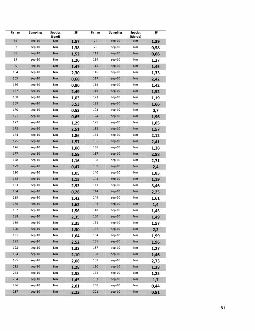
81
Fish nr Sampling Species (Sand)
ISF Fish nr Sampling Species (Riprap)
ISF
36 sep-10 Nm 1,57 74 sep-10 Nm 1,39
37 sep-10 Nm 1,38 75 sep-10 Nm 0,58
38 sep-10 Nm 1,52 113 sep-10 Nm 0,66
39 sep-10 Nm 1,20 114 sep-10 Nm 1,37
99 sep-10 Nm 1,47 115 sep-10 Nm 1,45
164 sep-10 Nm 2,30 116 sep-10 Nm 1,33
165 sep-10 Nm 0,68 117 sep-10 Nm 2,42
166 sep-10 Nm 0,90 118 sep-10 Nm 1,42
167 sep-10 Nm 2,49 119 sep-10 Nm 1,52
168 sep-10 Nm 1,03 121 sep-10 Nm 1,19
169 sep-10 Nm 3,53 122 sep-10 Nm 1,66
170 sep-10 Nm 0,53 123 sep-10 Nm 0,7
171 sep-10 Nm 0,65 124 sep-10 Nm 1,96
172 sep-10 Nm 1,29 125 sep-10 Nm 1,05
173 sep-10 Nm 2,51 132 sep-10 Nm 1,57
174 sep-10 Nm 1,86 133 sep-10 Nm 2,12
175 sep-10 Nm 1,57 135 sep-10 Nm 2,41
176 sep-10 Nm 1,00 136 sep-10 Nm 1,38
177 sep-10 Nm 1,59 137 sep-10 Nm 2,88
178 sep-10 Nm 1,16 138 sep-10 Nm 2,71
179 sep-10 Nm 0,47 139 sep-10 Nm 2,4
180 sep-10 Nm 1,05 140 sep-10 Nm 1,85
182 sep-10 Nm 1,15 141 sep-10 Nm 1,19
183 sep-10 Nm 2,93 143 sep-10 Nm 3,46
184 sep-10 Nm 0,28 144 sep-10 Nm 2,25
185 sep-10 Nm 1,42 145 sep-10 Nm 1,61
186 sep-10 Nm 1,62 146 sep-10 Nm 1,4
187 sep-10 Nm 1,56 148 sep-10 Nm 1,45
188 sep-10 Nm 2,35 150 sep-10 Nm 1,49
189 sep-10 Nm 2,35 151 sep-10 Nm 1,57
190 sep-10 Nm 1,30 152 sep-10 Nm 2,2
191 sep-10 Nm 1,64 154 sep-10 Nm 1,99
192 sep-10 Nm 2,52 155 sep-10 Nm 1,96
193 sep-10 Nm 1,33 157 sep-10 Nm 1,27
194 sep-10 Nm 2,10 158 sep-10 Nm 1,46
195 sep-10 Nm 2,08 159 sep-10 Nm 2,73
282 sep-10 Nm 1,28 160 sep-10 Nm 1,38
283 sep-10 Nm 2,58 162 sep-10 Nm 1,25
284 sep-10 Nm 1,45 163 sep-10 Nm 1,7
286 sep-10 Nm 2,01 200 sep-10 Nm 0,44
287 sep-10 Nm 2,23 201 sep-10 Nm 0,81

82
Fish nr Sampling Species (Sand)
ISF Fish nr Sampling Species (Riprap)
ISF
288 sep-10 Nm 2,08 202 sep-10 Nm 0,78
289 sep-10 Nm 1,98 203 sep-10 Nm 1,5
232 jul-11 Nm 1,13 204 sep-10 Nm 1,58
233 jul-11 Nm 3,40 205 sep-10 Nm 0,78
234 jul-11 Nm 2,05 206 sep-10 Nm 0,51
235 jul-11 Nm 1,06 207 sep-10 Nm 1,27
236 jul-11 Nm 2,87 246 sep-10 Nm 4,92
237 jul-11 Nm 1,18 247 sep-10 Nm 2,2
238 jul-11 Nm 2,72 248 sep-10 Nm 0,96
239 jul-11 Nm 2,54 249 sep-10 Nm 1,73
240 jul-11 Nm 1,55 251 sep-10 Nm 1,87
241 jul-11 Nm 1,51 252 sep-10 Nm 1,24
242 jul-11 Nm 1,43 254 sep-10 Nm 1,88
243 jul-11 Nm 1,14 255 sep-10 Nm 1,25
244 jul-11 Nm 2,05 256 sep-10 Nm 1,34
245 jul-11 Nm 1,49 290 sep-10 Nm 1,11
268 jul-11 Nm 1,72 291 sep-10 Nm 0,84
269 jul-11 Nm 1,94 292 sep-10 Nm 2,26
270 jul-11 Nm 2,36 208 jul-11 Nm 0,49
272 jul-11 Nm 1,81 209 jul-11 Nm 1,77
273 jul-11 Nm 3,08 210 jul-11 Nm 1,98
274 jul-11 Nm 2,17 211 jul-11 Nm 2,38
275 jul-11 Nm 1,96 212 jul-11 Nm 0,95
277 jul-11 Nm 2,48 213 jul-11 Nm 0,44
215 jul-11 Nm 1,66
216 jul-11 Nm 2,42
218 jul-11 Nm 0,44
219 jul-11 Nm 1,41
220 jul-11 Nm 0,44
221 jul-11 Nm 0,91
222 jul-11 Nm 2,38
223 jul-11 Nm 3,1
224 jul-11 Nm 1,47
225 jul-11 Nm 0,88
226 jul-11 Nm 1,92
227 jul-11 Nm 3,04
228 jul-11 Nm 0,96
229 jul-11 Nm 0,44
230 jul-11 Nm 1,35
231 jul-11 Nm 1,9
257 jul-11 Nm 3,28
83
Fish nr Sampling Species (Riprap)
ISF
258 jul-11 Nm 2,72
259 jul-11 Nm 2,22
260 jul-11 Nm 2,19
261 jul-11 Nm 1,4
262 jul-11 Nm 1,15
263 jul-11 Nm 1,61
264 jul-11 Nm 0,44
265 jul-11 Nm 0,45
266 jul-11 Nm 2,37
271 jul-11 Nm 3
278 jul-11 Nm 1,76
279 jul-11 Nm 2
280 jul-11 Nm 2,26
281 jul-11 Nm 0,76

84
Appendix 9: Stomach fullness index (ANOVA for significance)

85
Appendix 10: Correlation Stomach Fullness / Number of Parasites
Tab. H: Raw data of the number of parasites (N) for each category of the stomach fullness classification (cf. Tab 2)
SF classifi- cation
N Parasites
SF classifi- cation
N Parasites
SF classifi- cation
N Parasites
SF classifi- cation
N Parasites
SF classifi- cation
N Parasites
1 5 2 7 3 7 4 4 5 1 1 3 2 5 3 4 4 9 5 6 1 2 2 9 3 6 4 2 5 3 1 0 2 16 3 24 4 13 5 18 1 2 2 6 3 1 4 3 5 25 1 3 2 33 3 31 4 7 5 6 1 1 2 8 3 11 4 9 5 4 1 2 2 5 3 5 4 3 5 2 1 3 2 0 3 3 4 19 5 0 1 0 2 7 3 4 4 2 5 13 1 1 2 9 3 7 4 10 5 3 1 2 2 10 3 7 4 13 5 3 1 14 2 1 3 4 4 3 5 3 1 11 2 6 3 6 4 8 5 4 1 13 2 27 3 22 4 3 5 2 1 3 2 36 3 13 4 0 5 11 1 1 2 16 3 4 4 13 5 8 1 1 2 5 3 1 4 11 5 3 1 2 2 7 3 4 4 8 5 5 1 3 2 5 3 11 4 6 5 4 1 6 2 11 3 16 4 16 5 10 1 0 2 9 3 27 4 8 5 2 2 11 3 23 4 12 5 5 2 8 3 21 4 20 5 4 2 16 3 17 4 7 5 12 2 7 3 7 4 9 5 6 2 16 3 5 4 6 5 9 2 5 3 8 4 4 5 24 2 6 3 24 4 6 5 5 2 9 3 8 4 2 5 0 2 2 3 7 4 4 5 0 2 13 3 5 4 0 5 4 2 11 3 4 4 4 5 21 2 13 3 0 4 8 5 2 2 10 3 3 4 0 5 6 2 5 3 12 4 16 5 0 2 8 3 7 4 6 5 7 2 3 3 10 4 0 5 0 2 2 3 5 4 4 5 3 2 4 3 9 4 2 5 1 2 7 3 4 4 7 5 0 2 11 3 8 4 25 5 13

86
SF classifi- cation
N Parasites
SF classifi- cation
N Parasites
SF classifi- cation
N Parasites
SF classifi- cation
N Parasites
2 0 3 21 4 3 5 0 2 3 3 7 4 2 5 3 2 15 3 3 4 2 5 4 2 21 3 7 4 0 5 5 2 10 3 14 4 6 5 0 2 2 3 6 4 6 5 5 2 7 3 11 4 7 5 32 2 18 3 4 4 4 5 5 2 2 3 1 4 11 5 6 2 0 3 4 4 6 5 3 2 4 3 11 4 8 5 3 2 8 3 2 4 18 5 0 2 22 3 6 4 18 5 4 3 9 4 0 5 3 3 6 4 14 5 3 3 4 4 28 5 1 3 7 4 14 5 2 3 4 4 8 5 0 3 35 4 24 5 3 3 20 4 21 5 4 3 2 4 4 5 11 3 2 4 3 5 4 4 13 5 0 4 2 5 7 4 2 5 2 5 1 5 7 5 2 5 3 5 3

87
Appendix 11: Statistical analysis (correlation between number of parasites and fish)

88
Appendix 12: GSI values
Tab. I: Gonadosomatic index (GSI) of N. melanostomus (Nm) and P. kessleri (Pk) caught in the different habitats (sand; riprap) on July 2010. Fishes with a GSI value of 0% were excluded from the analysis.
Fish ID Habitat Species Sex Fish weight (g) Gonads GSI
89 Sand Nm f 9,8947 0,0089 0,09
95 Sand Nm f 5,1464 0,0417 0,82
99 Sand Nm f 8,6642 0,3393 4,08
100 Sand Nm f 6,9738 0,1297 1,90
110 Sand Nm f 5,3946 0,1809 3,37
111 Sand Nm f 6,3748 0,0236 0,37
90 Sand Nm m 17,4216 0,0381 0,22
93 Sand Nm m 12,3779 0,0103 0,08
98 Sand Nm m 13,8851 0,037 0,07
101 Sand Nm m 6,6471 0,2619 4,10
104 Sand Nm m 8,3746 0,0078 0,09
105 Sand Nm m 19,6976 0,04 0,20
112 Sand Nm m 35,1975 0,19 0,54
106 Riprap Nm m 24,6943 0,0341 0,14
108 Riprap Nm m 8,9082 0,0341 0,39
196 Riprap Nm m 9,2323 0,0948 1,04
198 Riprap Nm m 14,8024 0,0138 0,09
91 Riprap Pk f 32,0546 0,6982 2,23
109 Riprap Pk f 15,5511 0,0329 0,21
92 Riprap Pk m 19,1147 0,0363 0,19
Tab. J: Gonadosomatic index (GSI) of N. melanostomus (Nm) and P. kessleri (Pk) caught in the different habitats (sand; riprap) on September 2010. Fishes with a GSI value of 0% were excluded from the analysis.
Fish ID Habitat Species Sex Fish weight (g) Gonads GSI
26 Riprap Nm f 10,9989 0,0891 0,82
53 Riprap Nm f 7,6598 0,0029 0,04
54 Riprap Nm f 6,9607 0,0332 0,48
55 Riprap Nm f 9,0573 0,0091 0,10
58 Riprap Nm f 14,5486 0,0742 0,51
60 Riprap Nm f 29,3933 0,2152 0,74
70 Riprap Nm f 9,5711 0,0785 0,83
73 Riprap Nm f 11,9547 0,0654 0,55
75 Riprap Nm f 6,4974 0,0307 0,47
113 Riprap Nm f 18,8254 0,0892 0,48
115 Riprap Nm f 7,6408 0,0492 0,65
116 Riprap Nm f 14,8997 0,1144 0,77
117 Riprap Nm f 15,7648 0,0903 0,58
119 Riprap Nm f 5,5983 0,0051 0,09
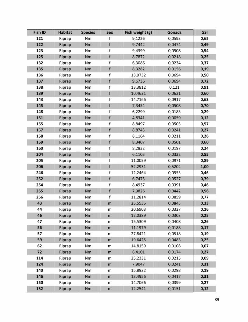
89
Fish ID Habitat Species Sex Fish weight (g) Gonads GSI
121 Riprap Nm f 9,1226 0,0593 0,65
122 Riprap Nm f 9,7442 0,0474 0,49
123 Riprap Nm f 9,4399 0,0508 0,54
125 Riprap Nm f 8,7872 0,0218 0,25
132 Riprap Nm f 6,3086 0,0234 0,37
135 Riprap Nm f 8,3282 0,0156 0,19
136 Riprap Nm f 13,9732 0,0694 0,50
137 Riprap Nm f 9,6736 0,0694 0,72
138 Riprap Nm f 13,3812 0,121 0,91
139 Riprap Nm f 10,4631 0,0621 0,60
143 Riprap Nm f 14,7166 0,0917 0,63
145 Riprap Nm f 7,3454 0,0508 0,70
148 Riprap Nm f 6,2299 0,0183 0,29
151 Riprap Nm f 4,8341 0,0059 0,12
155 Riprap Nm f 8,8497 0,0503 0,57
157 Riprap Nm f 8,8743 0,0241 0,27
158 Riprap Nm f 8,1164 0,0211 0,26
159 Riprap Nm f 8,3407 0,0501 0,60
160 Riprap Nm f 8,2832 0,0197 0,24
204 Riprap Nm f 6,1103 0,0332 0,55
205 Riprap Nm f 11,0059 0,0971 0,89
206 Riprap Nm f 52,2931 0,5202 1,00
246 Riprap Nm f 12,2464 0,0555 0,46
252 Riprap Nm f 6,7475 0,0527 0,79
254 Riprap Nm f 8,4937 0,0391 0,46
255 Riprap Nm f 7,9826 0,0442 0,56
256 Riprap Nm f 11,2814 0,0859 0,77
43 Riprap Nm m 25,5535 0,0843 0,33
44 Riprap Nm m 20,6903 0,0327 0,16
46 Riprap Nm m 12,0389 0,0303 0,25
47 Riprap Nm m 15,5309 0,0408 0,26
56 Riprap Nm m 11,1979 0,0188 0,17
57 Riprap Nm m 27,8421 0,0518 0,19
59 Riprap Nm m 19,6425 0,0483 0,25
62 Riprap Nm m 14,8159 0,0108 0,07
72 Riprap Nm m 6,4101 0,0174 0,27
114 Riprap Nm m 25,2331 0,0215 0,09
124 Riprap Nm m 7,9047 0,0241 0,31
140 Riprap Nm m 15,8922 0,0298 0,19
146 Riprap Nm m 13,4956 0,0417 0,31
150 Riprap Nm m 14,7066 0,0399 0,27
152 Riprap Nm m 12,2541 0,0151 0,12
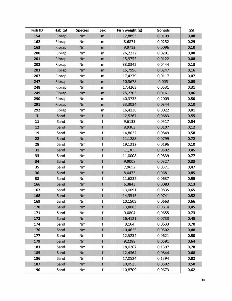
90
Fish ID Habitat Species Sex Fish weight (g) Gonads GSI
154 Riprap Nm m 12,8853 0,0109 0,08
162 Riprap Nm m 8,6871 0,0252 0,29
163 Riprap Nm m 9,9712 0,0096 0,10
200 Riprap Nm m 26,2232 0,0201 0,08
201 Riprap Nm m 15,9755 0,0122 0,08
202 Riprap Nm m 33,8342 0,0444 0,13
203 Riprap Nm m 15,7996 0,0247 0,16
207 Riprap Nm m 17,4279 0,0117 0,07
247 Riprap Nm m 10,3678 0,005 0,05
248 Riprap Nm m 17,4263 0,0531 0,31
249 Riprap Nm m 25,2703 0,0161 0,06
290 Riprap Nm m 40,3733 0,2009 0,50
291 Riprap Nm m 33,3024 0,0344 0,10
292 Riprap Nm m 16,4138 0,0022 0,01
3 Sand Nm f 12,5267 0,0683 0,55
11 Sand Nm f 9,6133 0,0517 0,54
12 Sand Nm f 8,9303 0,0107 0,12
19 Sand Nm f 14,8022 0,0849 0,58
22 Sand Nm f 11,1288 0,0799 0,72
28 Sand Nm f 19,1212 0,0196 0,10
31 Sand Nm f 11,305 0,0502 0,45
33 Sand Nm f 11,0008 0,0839 0,77
34 Sand Nm f 9,9008 0,0327 0,33
35 Sand Nm f 7,9652 0,0371 0,47
36 Sand Nm f 8,0473 0,0681 0,85
38 Sand Nm f 11,6832 0,0637 0,55
166 Sand Nm f 6,3843 0,0083 0,13
167 Sand Nm f 13,0091 0,0835 0,65
168 Sand Nm f 14,3513 0,0741 0,52
169 Sand Nm f 10,1509 0,0663 0,66
170 Sand Nm f 13,8083 0,0614 0,45
171 Sand Nm f 9,0804 0,0655 0,73
172 Sand Nm f 16,4121 0,0733 0,45
174 Sand Nm f 9,164 0,0633 0,70
176 Sand Nm f 10,4625 0,0502 0,48
177 Sand Nm f 12,5234 0,0621 0,50
179 Sand Nm f 9,2288 0,0591 0,64
183 Sand Nm f 18,0267 0,1397 0,78
185 Sand Nm f 12,4364 0,0844 0,68
186 Sand Nm f 17,0524 0,1394 0,82
187 Sand Nm f 10,0525 0,0502 0,50
190 Sand Nm f 10,8709 0,0673 0,62

91
Fish ID Habitat Species Sex Fish weight (g) Gonads GSI
192 Sand Nm f 8,9768 0,0599 0,67
193 Sand Nm f 16,1401 0,0689 0,43
194 Sand Nm f 12,7708 0,0621 0,49
20 Sand Nm m 13,5694 0,0901 0,67
29 Sand Nm m 26,2193 0,0811 0,31
30 Sand Nm m 13,3102 0,0804 0,61
37 Sand Nm m 11,9198 0,0256 0,22
39 Sand Nm m 10,0839 0,0739 0,74
164 Sand Nm m 17,9169 0,0238 0,13
165 Sand Nm m 11,5363 0,0247 0,21
178 Sand Nm m 9,4093 0,0013 0,01
180 Sand Nm m 20,6071 0,0142 0,07
182 Sand Nm m 4,5302 0,0042 0,09
184 Sand Nm m 33,1863 0,0599 0,18
189 Sand Nm m 17,9061 0,0288 0,16
282 Sand Nm m 27,7525 0,0236 0,09
283 Sand Nm m 24,0771 0,0301 0,13
284 Sand Nm m 35,3554 0,0994 0,28
286 Sand Nm m 17,1185 0,03 0,18
287 Sand Nm m 15,2133 0,0023 0,02
288 Sand Nm m 12,9029 0,0047 0,04
289 Sand Nm m 14,4254 0,0231 0,16
14 Riprap Pk f 7,2219 0,0259 0,36
18 Riprap Pk f 15,7032 0,1012 0,65
49 Riprap Pk f 20,9888 0,1652 0,79
51 Riprap Pk f 19,1205 0,1191 0,63
52 Riprap Pk f 16,7577 0,1371 0,82
61 Riprap Pk f 23,9526 0,1598 0,67
64 Riprap Pk f 23,1448 0,1315 0,57
67 Riprap Pk f 32,1674 0,2146 0,67
68 Riprap Pk f 25,8931 0,1747 0,68
84 Riprap Pk f 18,1318 0,0849 0,47
120 Riprap Pk f 16,6397 0,1207 0,73
142 Riprap Pk f 7,0245 0,0588 0,84
147 Riprap Pk f 44,7354 0,3916 0,88
156 Riprap Pk f 8,2261 0,0487 0,60
161 Riprap Pk f 6,4755 0,0361 0,56
250 Riprap Pk f 3,8699 0,0399 1,04
253 Riprap Pk f 24,0543 0,194 0,81
285 Riprap Pk f 21,7326 0,1718 0,80
21 Riprap Pk m 18,3844 0,1591 0,87

92
Fish ID Habitat Species Sex Fish weight (g) Gonads GSI
25 Riprap Pk m 17,5359 0,0767 0,44
42 Riprap Pk m 28,2962 0,2661 0,95
63 Riprap Pk m 21,4476 0,1339 0,63
66 Riprap Pk m 26,8047 0,0841 0,31
77 Riprap Pk m 34,0311 0,3287 0,98
129 Riprap Pk m 4,7931 0,0412 0,87
131 Riprap Pk m 30,7051 0,2024 0,66
149 Riprap Pk m 27,9583 0,2284 0,82 Tab. K: Gonadosomatic index (GSI) of N. melanostomus (Nm) and P. kessleri (Pk) caught in the different habitats (sand; riprap) on July 2011. Fishes with a GSI value of 0% were excluded from the analysis.
Fish ID Habitat Species Sex Fish weight (g) Gonads GSI
210 Riprap Nm f 5,8092 0,2181 3,90
211 Riprap Nm f 17,4519 0,3502 2,05
215 Riprap Nm f 6,4711 0,0241 0,37
216 Riprap Nm f 8,1825 0,1432 1,78
219 Riprap Nm f 5,7593 0,7102 14,07
221 Riprap Nm f 4,2037 0,6971 19,88
222 Riprap Nm f 4,6984 0,4158 9,71
223 Riprap Nm f 3,7879 0,4117 12,19
225 Riprap Nm f 17,2898 1,2181 7,58
227 Riprap Nm f 8,7732 0,0083 0,09
229 Riprap Nm f 3,4732 0,4007 13,04
230 Riprap Nm f 7,2819 0,0467 0,65
259 Riprap Nm f 4,5081 0,0871 1,97
260 Riprap Nm f 20,0741 0,9449 4,94
266 Riprap Nm f 7,3506 1,2596 20,68
278 Riprap Nm f 18,0097 0,3507 1,99
279 Riprap Nm f 6,7416 0,8155 13,76
208 Riprap Nm m 20,5962 0,3093 1,52
209 Riprap Nm m 17,1371 0,0854 0,50
212 Riprap Nm m 10,931 0,0316 0,29
213 Riprap Nm m 6,3819 0,0064 0,10
214 Riprap Nm m 12,4807 0,0304 0,24
218 Riprap Nm m 22,9598 0,6533 2,93
224 Riprap Nm m 10,4234 0,0164 0,16
226 Riprap Nm m 15,2755 0,0127 0,08
228 Riprap Nm m 20,1519 0,0383 0,19
257 Riprap Nm m 28,8908 0,8067 2,87
258 Riprap Nm m 12,8913 0,0186 0,14
261 Riprap Nm m 27,9865 0,0424 0,15
262 Riprap Nm m 13,487 0,0228 0,17

93
Fish ID Habitat Species Sex Fish weight (g) Gonads GSI
263 Riprap Nm m 9,5882 0,0112 0,12
264 Riprap Nm m 13,5659 0,2347 1,76
265 Riprap Nm m 8,1905 0,0143 0,17
281 Riprap Nm m 7,0301 0,0178 0,25
234 Sand Nm f 7,8654 0,3498 4,65
235 Sand Nm f 6,0901 0,8492 16,20
237 Sand Nm f 6,0213 0,7918 15,14
238 Sand Nm f 15,7872 0,8195 5,48
239 Sand Nm f 7,4829 0,1992 2,73
240 Sand Nm f 10,3832 1,1683 12,68
268 Sand Nm f 20,7578 0,3284 1,61
270 Sand Nm f 22,8924 0,0237 0,10
272 Sand Nm f 14,1022 0,3923 2,86
277 Sand Nm f 4,4457 0,4079 10,10
232 Sand Nm m 11,5567 0,02 0,17
233 Sand Nm m 15,9848 0,0387 0,24
236 Sand Nm m 12,2309 0,0383 0,31
241 Sand Nm m 10,7463 0,3801 3,67
242 Sand Nm m 12,3509 0,0153 0,12
243 Sand Nm m 11,5406 0,0153 0,13
244 Sand Nm m 9,5498 0,0172 0,18
245 Sand Nm m 17,6052 0,0274 0,16
269 Sand Nm m 11,3133 0,0183 0,16
273 Sand Nm m 8,0359 0,0173 0,22
274 Sand Nm m 9,2778 0,0154 0,17
275 Sand Nm m 7,5958 0,0103 0,14
271 Riprap Pk f 5,0851 0,8073 18,87

94
Appendix 13: Parasite infection (N) per individual Table L: Number of parasites for each infected individual (ID Number) of Neogobius melanostomus in the two different habitats (with mean values) at each sampling date
Sample ID number Sand ID number Riprap
Nm Jul 2010 89 1 93 3 90 3 98 0 94 3 99 3 95 1 100 2 96 13 101 1 97 2 102 2
103 3 106 6 104 1 107 1 105 5 197 9 108 7 Mean: 3.4 110 2 111 2 112 14 196 5 198 16 199 6
Mean: 5.3
Sample ID number Sand ID number Riprap Nm Sep 2010 1 27 3 16
2 36 4 5 5 7 11 8 6 5 12 16 7 11 19 27 8 9 22 17 9 11 24 5
10 13 26 24 13 7 28 15 16 4 33 18 17 11 34 2 20 23 35 1 23 7 47 20 27 8 50 6 29 21 53 2 30 10 54 4 31 2 57 11 38 22 58 6 41 11 70 3 43 7 72 2 48 7 73 2 56 4 75 6 59 8 78 25 60 18 79 6
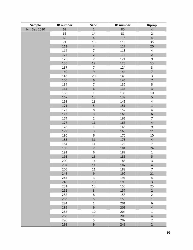
95
Sample ID number Sand ID number Riprap Nm Sep 2010 62 1 80 4
65 14 81 2 69 4 115 4 71 13 116 35
113 4 117 20 114 7 118 4 122 2 119 2 125 7 121 9 136 12 123 13 137 7 124 3 140 9 144 7 143 20 145 3 150 6 146 7 154 7 132 5 164 6 135 3 166 1 138 10 167 13 139 5 169 13 141 4 171 5 151 1 172 8 152 4 173 3 160 6 174 2 162 7 177 11 163 4 178 1 165 9 179 3 168 11 180 6 170 10 183 31 175 4 184 11 176 7 189 7 181 24 191 6 182 1 193 13 185 5 200 14 186 3 202 11 187 4 206 11 188 7 246 9 192 21 247 3 194 4 248 19 195 3 251 13 155 25 252 3 157 2 282 8 158 2 283 5 159 1 284 1 201 6 286 9 203 4 287 10 204 1 288 1 205 4 290 5 207 2 291 9 249 2
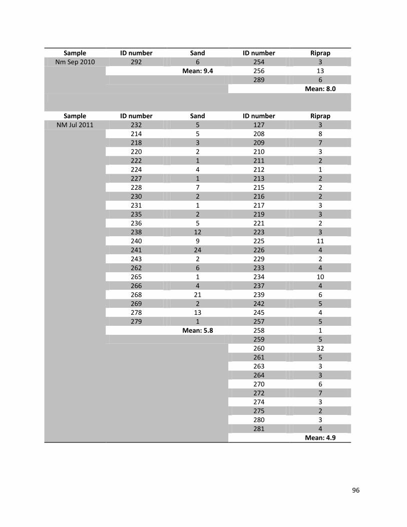
96
Sample ID number Sand ID number Riprap Nm Sep 2010 292 6 254 3
Mean: 9.4 256 13 289 6
Mean: 8.0
Sample ID number Sand ID number Riprap NM Jul 2011 232 5 127 3
214 5 208 8 218 3 209 7 220 2 210 3 222 1 211 2 224 4 212 1 227 1 213 2 228 7 215 2 230 2 216 2 231 1 217 3 235 2 219 3 236 5 221 2 238 12 223 3 240 9 225 11 241 24 226 4 243 2 229 2 262 6 233 4 265 1 234 10 266 4 237 4 268 21 239 6 269 2 242 5 278 13 245 4 279 1 257 5
Mean: 5.8 258 1 259 5
260 32 261 5 263 3 264 3 270 6 272 7 274 3 275 2 280 3 281 4
Mean: 4.9

97
Appendix 14: Morphology (ANOVA for significance)
One-way ANOVA analysis for testing the influences of the variable habitat (at different sampling dates
and between all dates together) on changes in the morphology of Neogobius melanostomus.
Table M: One way ANOVA for testing the influence of variable haitat on maximal head length (MHL) and maximal body width (MBW).The mean difference is significant at the 0.05 level.
Sampling
Date
Source Dependent
variable
df Mean
Square
F Sig
22. Jul 2010 Habitat MHL 1 6.143 0.4 0.5333
MBW 1 5.3814 0.39 0.5385
14. Sep 2010 Habitat MHL 1 3.489 0.44 0.4487
MBW 1 3.8538 0.47 0.4941
5. Jul 2011 Habitat MHL 1 1.4142 0.16 0.6906
MBW 1 2.9582 0.37 0.5454
All Habitat MHL 5 11.7361 1.48 0.2112
MBW 5 13.3012 1.41 0.2326