Dissertations and Theses

5-2014

The Effect of the 2-Dimensional Magnetic Field Profile in Hall The Effect of the 2-Dimensional Magnetic Field Profile in Hall

Thrusters Thrusters

Megan Lewis Harvey Embry-Riddle Aeronautical University - Daytona Beach

Follow this and additional works at: https://commons.erau.edu/edt

Part of the Propulsion and Power Commons, and the Space Vehicles Commons

Scholarly Commons Citation Scholarly Commons Citation Harvey, Megan Lewis, "The Effect of the 2-Dimensional Magnetic Field Profile in Hall Thrusters" (2014). Dissertations and Theses. 160. https://commons.erau.edu/edt/160

This Thesis - Open Access is brought to you for free and open access by Scholarly Commons. It has been accepted for inclusion in Dissertations and Theses by an authorized administrator of Scholarly Commons. For more information, please contact commons@erau.edu.

THE EFFECT OF THE 2-DIMENSIONAL MAGNETIC FIELD

PROFILE IN HALL THRUSTERS

By

Megan Lewis Harvey

A Thesis Submitted to the

Department of Physical Sciences

In Partial Fulfillment of the Requirements for the Degree of

Master of Science in Engineering Physics

Embry-Riddle Aeronautical University

Daytona Beach, Florida

May 2014

c© Copyright by Megan Lewis Harvey 2014

All Rights Reserved

ii

Abstract

Electric propulsion engines, in particular Hall thrusters, provide the possibility of

long-distance, low-cost space traval. The geometrical details of the Hall thrusters,

especially the magnetic field profile, are crucial to improving their efficiency. The

effect of the magnetic field structure was investigated using a simple, two-dimensional

model, assuming axial symmetry. The previous one-dimensional conclusion, namely

that the details of the shape of the magnetic field are unimportant, was confirmed.

This result has implications for the design of future Hall thruster engines, with an

eye toward maximizing their efficiency.

iv

Acknowledgments

First and foremost, I would like to thank my thesis advisor, Dr. Mark Anthony

Reynolds. Without his willingness to stick with me and this topic, I would not have

been able to finish writing. Even after I moved halfway across the country, he always

responded to my emails (no matter how frequent or infrequent) with helpful edits

and an encouraging word. You have my deepest gratitude for not giving up on me.

I would also like thank the rest of my thesis committee, Dr. John Hughes and Dr.

Bereket Berhane. You have not only been generous with your time to participate

in my defense process, but each of you made a lasting contribution to my education

during my three years at ERAU. Also, yes, I did leave before I was finished. It was

just as hard as you all told me it would be. You are all welcome to give me as many

“I told ya so”s as you please. I must also acknowledge Oren Kornberg, upon whose

research this paper was based. I’ve never met you, but you created a great jumping-

off point into another whole dimension. Finally, thank you to my boyfriend, Aaron,

and especially, my parents. You never stopped believing in me, and your faith and

love have always gotten me through the toughest moments. xo.

v

Contents

Abstract iv

Acknowledgments v

1 Introduction 1

1.1 Thruster Principles . . . . . . . . . . . . . . . . . . . . . . . . . . . . 3

1.2 Hall Thruster Design . . . . . . . . . . . . . . . . . . . . . . . . . . . 4

1.2.1 The Hall Effect . . . . . . . . . . . . . . . . . . . . . . . . . . 6

2 Methodology 9

2.1 Governing equations . . . . . . . . . . . . . . . . . . . . . . . . . . . 10

2.1.1 1-D Model . . . . . . . . . . . . . . . . . . . . . . . . . . . . . 12

3 Results 22

3.1 Approximation of constant B . . . . . . . . . . . . . . . . . . . . . . 25

3.1.1 Energy . . . . . . . . . . . . . . . . . . . . . . . . . . . . . . . 27

3.1.2 Momentum . . . . . . . . . . . . . . . . . . . . . . . . . . . . 29

3.2 Numerical Results . . . . . . . . . . . . . . . . . . . . . . . . . . . . . 30

4 Conclusion 33

vi

A Numerical Methods 35

A MATLAB code 39

A.1 Define Differential Equation with Simple B . . . . . . . . . . . . . . . 39

A.2 Define Differential Equation with Varying B . . . . . . . . . . . . . . 39

A.3 Plot Results . . . . . . . . . . . . . . . . . . . . . . . . . . . . . . . . 40

Bibliography 43

vii

List of Figures

1.1 Cutaway view of a Hall thruster. This model schematic shows the

configuration of electric and magnetic field lines as well as the definition

of the annulus width, W , and typical particle trajectories. [9] . . . . . 5

1.2 Cycloid motion of charged particles in an environment of perpendicular

electric and magnetic fields. [11] . . . . . . . . . . . . . . . . . . . . . 7

2.1 Solutions of the second order ODE (Ordinary Differential Equation)

for five different f-values, each related to a different constant magnetic

field strength. Weaker magnetic fields result in a potential (φ) drop at

a longer axial distance (z) than stronger magnetic fields. . . . . . . . 20

2.2 The length of the acceleration region changes for different average mag-

netic field values. . . . . . . . . . . . . . . . . . . . . . . . . . . . . . 21

3.1 Electric potential along the acceleration region plotted at various radii.

R1 corresponds to the inner radius, and R2 to the outer radius of the

annular chamber of the Hall Thruster. . . . . . . . . . . . . . . . . . 23

3.2 Electric potential at the end of the acceleration region at different

radius values, where r is the radius scaled to R1 . . . . . . . . . . . . 24

viii

3.3 Comparison of two different aspect ratios (R2

R1). The smaller ratio re-

sults in a smaller spread of magnetic field values. . . . . . . . . . . . 25

3.4 Area of annular region at various aspect ratios normalized to the area

with the largest aspect ratio. With increasing aspect ratio, the area of

the annulus at the end of the acceleration region increases. . . . . . . 26

3.5 Energy (normalized to energy emitted with the largest aspect ratio)

emitted by the system at various aspect ratios for a constant magnetic

field. . . . . . . . . . . . . . . . . . . . . . . . . . . . . . . . . . . . . 27

3.6 Momentum (normalized to momentum produced with the largest as-

pect ratio) at various aspect ratios for a constant magnetic field. . . . 28

3.7 Momentum versus energy (each normalized to their greatest values)

emitted by the system for a constant magnetic field. . . . . . . . . . . 29

3.8 Comparison of the energy emitted by the system at various aspect

ratios for constant, increasing, and decreasing magnetic fields. . . . . 31

3.9 Comparison of the momentum of the system at various aspect ratios

for constant, increasing, and decreasing magnetic fields. . . . . . . . . 32

3.10 Momentum versus energy emitted by the system at various aspect ra-

tios for constant, increasing, and decreasing magnetic fields. . . . . . 32

A.1 Two coupled first order ODEs calculating length of potential drop

in the acceleration chamber solved with a fourth-order Runge Kutta

method. Five different f-values are plotted, each related to a different

constant magnetic field. . . . . . . . . . . . . . . . . . . . . . . . . . 36

A.2 Log-log plot of error of the coupled first-order ODEs between RK4 and

AMB methods. . . . . . . . . . . . . . . . . . . . . . . . . . . . . . . 36

ix

A.3 Log-log plot of error of the coupled first-order ODEs between RK4 and

Modified Midpoint methods. . . . . . . . . . . . . . . . . . . . . . . . 37

A.4 Log-log plot of error between the coupled first-order ODEs and the

second order ODE both solved with RK4. . . . . . . . . . . . . . . . 37

A.5 Log-log plot of error between the coupled first-order ODEs solved with

RK4 and the second order ODE solved with AMB. . . . . . . . . . . 38

A.6 Log-log plot of error between the coupled first-order ODEs solved with

RK4 and the second order ODE solved with Modified Midpoint. . . . 38

x

Chapter 1

Introduction

Space, the final frontier, is a fascinating, slowly unfolding mystery for all of mankind.

The last century has given rise to a swift acceleration in technology and discovery.

Humans have constructed a vast and complex near-earth system of satellites, we

have sent probes to explore all 8 major planets, transported 24 men to Earth’s moon

and back, and we even have a spacecraft traveling far past Pluto, through our solar

system’s heliosheath, that is still returning a signal. There is an aspect of space

exploration common to all these accomplishments: propulsion. Maximizing efficiency

is an ever-important aspect in the design process, and harnessing the Hall Effect for

thruster applications that necessitate long travel time or high exhaust velocity outside

Earth’s atmosphere is an effective method. This study’s focus is the optimization of

a Hall Effect Thruster’s magnetic field structure in two dimensions.

Hall Effect Thrusters are one type of electric propulsion where a non-reactive gas

takes the form of a plasma with enough conductivity to sustain current and react

to electric and magnetic fields. The benefit of electric propulsion is that the fuel to

mass ratio can be very low. However, the disadvantage is low thrust. Therefore,

1

CHAPTER 1. INTRODUCTION 2

electric propulsion engines are only good for long, low-thrust (but high change in

velocity, ∆v) missions far from the strong gravitational influence of planets. A goal

this project and any thruster design is to make the thrust as large as possible for as

low an energy input as possible.

Robert Goddard first introduced the concept of electric propulsion in his notebook

in February of 1906 [13]. He observed that charged particles took on very high

velocities in an electric gas discharge tube. The tube remained at a relatively low

temperature, and he conjectured that this may be the answer to his hope for achieving

high exhaust velocity. A higher exhaust velocity allows for a greater ∆v and allows

for a vehicle to have a large payload mass fraction.

The United States and Russia began more in depth research into the subject

of electric propulsion in the 1960’s. Russia was the first to employ an extensive

fleet of Hall Thrusters on their communication satellites for station keeping purposes

starting in 1971[7]. It took until the 1990’s for electric propulsion design to be suitably

advanced to fly commercially. The European Space Agency’s SMART-I was arguably

the most high profile spacecraft to employ a Stationary Plasma Hall Effect Thruster,

capable of producing thrust upwards of 70 milliNewtons [1].

Electric propulsion engines, in particular Hall thrusters, provide the possibility of

long-distance, low-cost space traval. The geometrical details of the Hall thrusters,

especially the magnetic field profile, are crucial to improving their efficiency. In this

Chapter we will discuss thruster principles in general, and explore specifics in Hall

thruster design and the Hall Effect that drives this type of electric propulsion. Chap-

ter Two delves into how plasma in the thruster is characterized through governing

equations in one-dimension. From there, the model is relaxed to two-dimensions and

CHAPTER 1. INTRODUCTION 3

the effect of the magnetic field structure is investigated. In Chapter Three, results

show that the previous one-dimensional conclusion, namely that the details of the

shape of the magnetic field are unimportant, holds up in two dimensions. This result

has implications for the design of future Hall thruster engines, with an eye toward

maximizing their efficiency. Chapter Four summarizes the conclusion.

1.1 Thruster Principles

In any rocket engine, thrust is created by ejecting mass to propel a spacecraft. It is

defined in the following equation

T = Mpropvex, (1.1)

where Mprop is the mass flow rate of the propellant and vex is the exhaust velocity

[7]of the propellant relative to the engine. In the case of electric propulsion, the mass

consists of energetic charged particles. The propellant mass flow rate is defined as

Mprop = Qm (1.2)

where Q is the the propellant particle flow rate and m is the mass of each particle.

Mprop is essentially a rocket engine’s fuel consumption rate, and the amount of thrust

able to be produced by a certain mass flow rate is analogous to its fuel efficiency.

This efficiency is given by specific impulse, or Isp, and for constant thrust,T ,and

CHAPTER 1. INTRODUCTION 4

propellant flow rate is defined as

Isp =T

Mpropg, (1.3)

where g is the acceleration due to gravity. Using Equation (1.1), specific impulse can

be rewritten as

Isp =vexg. (1.4)

With electric propulsion engines guaranteeing a much higher exhaust velocity than

their chemical counterparts, they can in turn provide much higher specific impulse

(1500-2000 s for Hall thrusters versus 150-450 s for chemical [7]) and are much more

propellant-efficient.

1.2 Hall Thruster Design

Figure 1.1 shows a schematic of a typical Hall Thruster. A heavy, non-reactive gas

such as Xenon is fed into an annular chamber. Centered inside and surrounding

this chamber are electromagnets, creating a radial magnetic field. An electric field is

created by an electric potential difference between an anode and cathode pair in the

axial direction. The perpendicular fields, axial electric and radial magnetic, cause the

electrons fed by the cathode to become trapped, gyrating around the magnetic field

lines and drifting around the acceleration chamber azimuthally. This flow of electrons

as a result of the orthogonal configuration of electric and magnetic fields is known as

the Hall Effect.

CHAPTER 1. INTRODUCTION 5

Figure 1.1: Cutaway view of a Hall thruster. This model schematic shows the con-figuration of electric and magnetic field lines as well as the definition of the annuluswidth, W , and typical particle trajectories. [9]

CHAPTER 1. INTRODUCTION 6

1.2.1 The Hall Effect

E. H. Hall discovered this effect in 1879 by running a current through a piece of

conducting gold foil while simultaneously creating a magnetic field perpendicular to

the current flow. Perpendicular to both fields he found that a potential difference

was created [8].

In a uniform magnetic field with no electric field present, the equation of motion

for a single charged particle is given by Newton’s Second Law,

mdv

dt= qv ×B, (1.5)

where v is the velocity of the particle, q is its charge, B is the magnetic field, m is

the mass of the particle, and qv ×B is the Lorentz force acting on the particle.

Each particle orbits around a guiding center with a frequency dependent on mass

ωc ≡|q|Bm

(1.6)

where ωc is called the cyclotron frequency.

The cyclotron radius, rc, of these orbits also depends on mass

rc ≡v⊥ωc

=mv⊥|q|B

(1.7)

where v⊥ is the velocity of the particle perpendicular to the magnetic field. No-

ticeably, ions will have a lower cyclotron frequency and larger cyclotron radius than

electrons because of their larger mass. In this environment, seen in Figure 1.2, posi-

tively charged particles will rotate clockwise around the magnetic field, and negative

CHAPTER 1. INTRODUCTION 7

particles will move counterclockwise [9].

Figure 1.2: Cycloid motion of charged particles in an environment of perpendicularelectric and magnetic fields. [11]

In the annular region of the thruster, it is essential to design the width (W ) of the

annulus in a way to allow the distinct electron and ion properties to be exploited. This

width must be significantly smaller than the ion’s cyclotron radius so that ions may

be free to accelerate through the axial potential drop. [9] W must also be significantly

larger than the electron’s cyclotron radius in order to restrict the electron’s movement,

so

W rc, ion and W rc, electron. (1.8)

This restriction keeps the electrons in the annular region, able to continually ionize

the incoming Xenon particles.

When a finite electric field is also present, the Lorentz force defines the particle’s

equation of motion

mdv

dt= q(E + v ×B). (1.9)

Here, a particle’s guiding center, vgc, drifts perpendicular to both fields with a velocity

CHAPTER 1. INTRODUCTION 8

defined as

vgc ≡E ×B

B2, (1.10)

and known as the “E cross B” drift. As such, the particle travels in a helical path.

Within the plasma in a Hall Thruster, the collisions between particles become an

important property. This is parametrized as the Hall parameter, ΩH , which is a ratio

of the cyclotron frequency ωc and the collision frequency νc [9]:

ΩH =ωcνc. (1.11)

It is a measure of how a particle’s motion will be characterized. A large Hall parameter

would allow a particle’s azimuthal orbit to be much less perturbed by collisions,

whereas a particle operating under a low Hall parameter will be subject to many

more collisions that will interrupt each cyclotron orbit.[10] This parameter is the key

to allowing the low ΩH ions to behave like a fluid while keeping the high ΩH electrons

trapped and E ×B drifting in the azimuthal direction.

Chapter 2

Methodology

Exploration of the dependence of efficiency and thrust on different variables has lead

to many studies concerning the steady state physics of the plasma within a Hall

thruster’s acceleration region (for example, Fruchtman and Fisch, 1998 [6]). Al-

though the equilibrium plasma configuration is inherently three-dimensional, simple

1-D theoretical models such as those developed by Ahedo et al., 2001 [2] and Choueiri,

2001 [4], can distill the basic physical properties without a full Magnetohydrodynamic

(MHD) simulation.

It is clear that the structure of the magnetic field is important. Specifically,

the azimuthal profile of the radial component of B affects efficiency. Kornberg [11]

investigated how the shape of the magnetic field affects the length of the acceleration

region. He concluded that this length is only weakly dependent on the shape of

the magnetic field profile, but the average value of the magnetic field is inversely

proportional to acceleration region length.

Here, we will expand Kornberg’s analysis to two dimensions to see if a similar

conclusion persists. From a simple model without the full MHD simulation we find

9

CHAPTER 2. METHODOLOGY 10

that in fact, that when the average magnetic field is held constant, a variation of it’s

shape along the length of the Hall Thruster does not have an appreciable impact on

the thrust of the engine.

To that end, we begin with summarizing Choueiri’s model from 2001 [4], as

generalized by Kornberg. In the following chapter we present our simplified two-

dimensional extension and the results on the relationship between magnetic field and

the length of the acceleration region.

2.1 Governing equations

To explore the properties of the plasma inside the Hall thruster acceleration region,

we begin with the generalized fluid equations.

The momentum equation is essentially Newton’s Second Law normalized per unit

volume,

mn

[(∂v

∂t

)+ (v ·∇)v

]= −∇p+ qn(E + v ×B)− mn(v − v0)

τ, (2.1)

where n is the number density of the particle, p is the pressure, v0 is the velocity

of the neutral fluid, and τ is the average time between collisions. The left-hand-side

of this equation includes the so-called “convective derivative”, and the terms on the

right-hand-side are the forces: the pressure gradient, the Lorentz force, and frictional

drag. [11]

The second fluid equation used is the continuity equation, which states that the

rate at which particles enter a system must be equal to the rate at which the particles

CHAPTER 2. METHODOLOGY 11

leave,

∂n

∂t+∇ · (nv) = Sα. (2.2)

Sα is the source term for particles that governs the properties of ionization, recombi-

nation, and thruster wall attachment, where α represents each type of particle species.

The following equations show the electron, ion, and neutral source terms [11],

Se = kine − krn2e − kane, (2.3)

Si = kini − krn2i − kani, (2.4)

Sn = krn2e − kine, (2.5)

where ki, kr, and ka are the ionization, recombination, and thruster wall attachment

coefficients, respectively.

In addition to the fluid equations, Maxwell’s equations are needed to completely

characterize the system. First is Gauss’s Law,

εo(∇ ·E) = ρ, (2.6)

where εo is the permittivity of free space, and ρ is the electric charge density,

ρ =∑

qn = e(ni − ne), (2.7)

where e = 1.602× 10−19 C is the charge of an electron. For this study, electric charge

density, ρ, is negligible due to the assumption of quasi-neutrality, ni ≈ ne. From this

point forward, particle density will simply be referred to as n.

CHAPTER 2. METHODOLOGY 12

Ampere’s Law states

∇×B = µ0J , (2.8)

where µ0 is the permeability of free space, and J is the current density. This will be

expanded later to show how the strength of the magnetic field changes. Maxwell’s

addition of the displacement current is not included here as this is a steady-state

study and the displacement current based on ∂E∂t

.

Finally, Gauss’s Law for magnetic fields states that the divergence of the magnetic

field is equal to zero,

∇ ·B = 0. (2.9)

The solution to this equation in cylindrical coordinates is

Br =B0R0

r(2.10)

where Br = B0 at r = R0.

2.1.1 1-D Model

Following the work of Kornberg[11] and Choueiri[4], simplifications must be made to

the fluid equations to reflect a steady state system with no variation in the radial

direction.

Reflecting these simplifications and multiplying both sides by e, Equation (2.2)

becomes the electron-specific continuity equation

djezdz

= kine, (2.11)

CHAPTER 2. METHODOLOGY 13

where jez = nevez, and kine is the rate of ionization, and ki is the ionization coefficient.

The left hand side above is what remains from the divergence term in Equation

(2.2), and the right hand side is the ionization term of the electron source term from

Equation (2.3). This equality defines that the rate of electrons introduced into the

Hall thruster’s annular chamber is equal to the rate of electron ionization.

The ion-specific continuity equation is

∇ · ji = 0. (2.12)

The divergence of the ion current is equal to zero because we assume that pressure

is low and the ion current current far exceeds the electron current, so the collision

term is negligible. And because the divergence is equal to zero, the current in the

z-direction must be a constant. We will define this constant as ji0, the ion current at

the end of the acceleration channel [11].

We can impose energy conservation on the ion fluid,

1

2miv

2i = e(φa − φ), (2.13)

where φ is the electric potential, φa is the electric potential at the anode, where the

ions are at rest. Solving Equation (2.12) for density, and then substituting in vi from

the energy equation yields the electron number density,

n =ji0

e√

2e(φa−φ)mi

. (2.14)

The momentum equation (2.1) is simplified for electrons into two components.

CHAPTER 2. METHODOLOGY 14

The z-component is

neveθBr +menνcvez = −dpdz

+ neEz, (2.15)

where νc = 1τ

is the the collision frequency, and me = 9.109× 10−31 kg is the mass of

an electron,

The azimuthal component allows for comparison of the azimuthal velocity to axial

velocity,

0 = envezBr −mnνcveθ. (2.16)

Solving for veθ gives

veθ = vezeBr

mνc= vezΩHe, (2.17)

where eBm

= ωce, the electron cyclotron frequency or gyrofrequency, and ωceνc

= ΩHe,

the electron Hall parameter. Remember from Chapter 1 that Hall thrusters thrive on

electrons with a large Hall parameter. This results in few neutral collions, keeping

electrons in the acceleration region, able to continually ionize incoming neutral gas.

Substituting p = nT (from the ideal gas law that holds true for cold plasmas

[14]), where T is temperature (technically, T here is the product of the Boltzman

constant and temperature, kT , since we are dealing with energy at the molecular-

scale), veθBr = vezBrΩHe, Ez = dφdz

, and factoring out nevz from the left hand side of

Equation (2.15) gives

jez

(BrΩHe +

meνce

)= ne

dφ

dz− d(nT )

dz. (2.18)

The inverse of the term inside of the parentheses on the left hand side above

CHAPTER 2. METHODOLOGY 15

becomes

e

meνc

1BrΩHemeνc

+ 1. (2.19)

This is defined as the Pederson mobility,

µe =e

meνc

1

Ω2He + 1

. (2.20)

This mobility is the proportionality constant between a charged particle’s velocity

and the applied electric field. [11] It characterizes how quickly an electron can move

when under the electric field’s influence.

The simplified electron momentum equation finally becomes,

jz = µe

(nedφ

dz− d(nT )

dz

). (2.21)

Energy

Choueiri [4] suggests a very simple assumption for energy,

Te = βeφ, (2.22)

where β is a constant between 0 and 1. This equation states that the electron energy

increases linearly with the potential as they move through the acceleration chamber,

from cathode to anode. The physical justification for this approximation is that as

electrons collide with neutrals, some of their directed kinetic energy is converted into

random thermal energy. This fraction of potential energy gained by the electrons

(β) heats the plasma, and the temperature increases with increasing potential. As

Kornberg [11] states, it is not strictly correct, but is sufficient to complete the system

CHAPTER 2. METHODOLOGY 16

of equations.

Scaling

Equations (2.11), (2.14), (2.21), and (2.22) above are scaled (as developed by Korn-

berg [11]) to reduce the number of constants using the following definitions,

φ ≡ φ

φa, z ≡ z

l′, n ≡ n

n′, jez ≡

jezj′, (2.23)

T ≡ T

eφa, f(z) ≡ B(z)

B′, Ωe(z) =

eB′

meνcf(z), (2.24)

where B′ is chosen such that, B′ = meνce

and therefore Ωe(z) = f(z) and f(z) =

emeνc

B(z) 1.

This results in the following dimensionless equations,

djezdz

= Qn, (2.26)

n = A(1− φ)−12 , (2.27)

1The dimensionless magnetic field is important to take into consideration, and its coefficient isdefined as γ = eB′

meνc, where the collision frequency is

νc = naσve, (2.25)

where na ≈ 1016m−3 [3] is the number density for Xenon, σ = πr2vdw is the cross sectional areaof collisions, where r2vdw = 2.17 × 10−10m2 is the Van der Waals radius for Xenon [5], so that

σ = 1.48×10−19m2. ve ≈√

8kTe

πmeis the average electron velocity where kTe = 10eV = 1.6×10−18J ,

so that ve ≈ 2.1× 106m/s. This makes νc = 3.15× 104s−1, so the coefficient of the magnetic field,γ = 5.59× 106Cskg .

CHAPTER 2. METHODOLOGY 17

jez = C(z)[ndφ

dz− d(nT )

dz

], (2.28)

and

T = βφ, (2.29)

where

Q =kiel

′n′

j′, A =

ji0

n′e√

2eφame

, C(z) = µe(z)eφan

′

l′j′, (2.30)

and

µe(z) = µ01

1 + f 2(z), (2.31)

where

µ0 =e

meνc. (2.32)

Equations (2.26) through (2.29) can be combined to form two first order ordinary

differential equations,

d¯jezA

dz=

Q

(1− φ)12

(2.33)

dφ

dz=

¯jezAC(z)

(1− φ)32

1− φ− β(1− φ2), (2.34)

or one second order differential equation,

d2

dz2

[2(1− φ)1/2 + (1− φ)−1/2βφ

]+

Q

C(z)(1− φ)−1/2 = 0. (2.35)

CHAPTER 2. METHODOLOGY 18

Kornberg defined the coefficient of the last term in this equation as follows [11],

λ(z) ≡ Q

C(z). (2.36)

Expanding QC(z)

yields

Q

C(z)=ki(l

′)2

µeφa(1 + f 2). (2.37)

Choosing l′ =√

µeφaki

, conveniently results in the coefficient of 1 + f 2 equaling

unity.

Consequently, λ is dimensionless and inversely proportional to electron mobility,

λ(z) = 1 + f 2 ∝ 1

µe. (2.38)

This equivalency is adopted and used to solve the second order differential equation

for the second derivative of φ,

d2φ

dz2=

(dφdz

)2

2

[(1− φ)−1 − β(1− φ)−1 − 3

2βφ(1− φ)−2 − β(1− φ)−1 − 2(1+f2)

φ2

]β − 1 + β

2φ(1− φ)−1

(2.39)

Exploration of the numerical solutions for these differential equations can be found

in Appendix A. MATLAB’s fourth order Runge-Kutta solver was sufficient for solving

the second order differential equation. It is a non-linear ordinary differential equation

for the electric potential, φ, as a function of axial position, z. The constant, β, from

Choueiri’s energy relation, Equation (2.22), is set to β = 0, using the cold plasma

approximation. Future work could look at how varying β could change the potential

profile.

CHAPTER 2. METHODOLOGY 19

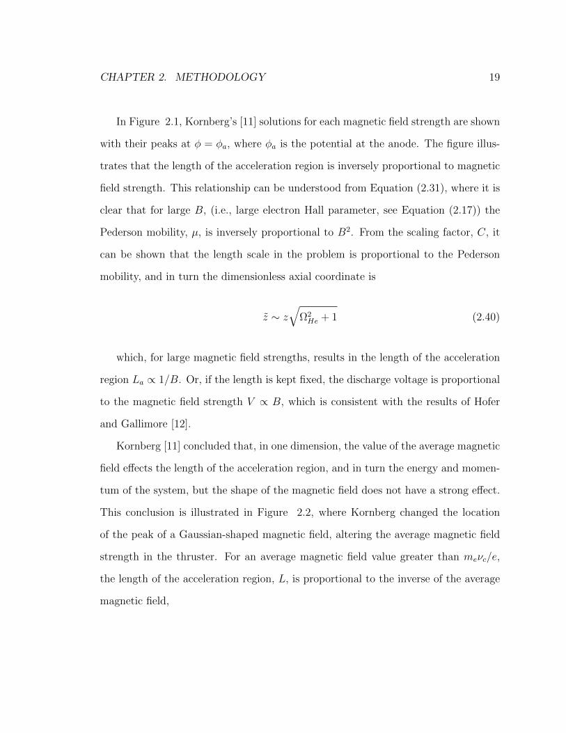
In Figure 2.1, Kornberg’s [11] solutions for each magnetic field strength are shown

with their peaks at φ = φa, where φa is the potential at the anode. The figure illus-

trates that the length of the acceleration region is inversely proportional to magnetic

field strength. This relationship can be understood from Equation (2.31), where it is

clear that for large B, (i.e., large electron Hall parameter, see Equation (2.17)) the

Pederson mobility, µ, is inversely proportional to B2. From the scaling factor, C, it

can be shown that the length scale in the problem is proportional to the Pederson

mobility, and in turn the dimensionless axial coordinate is

z ∼ z√

Ω2He + 1 (2.40)

which, for large magnetic field strengths, results in the length of the acceleration

region La ∝ 1/B. Or, if the length is kept fixed, the discharge voltage is proportional

to the magnetic field strength V ∝ B, which is consistent with the results of Hofer

and Gallimore [12].

Kornberg [11] concluded that, in one dimension, the value of the average magnetic

field effects the length of the acceleration region, and in turn the energy and momen-

tum of the system, but the shape of the magnetic field does not have a strong effect.

This conclusion is illustrated in Figure 2.2, where Kornberg changed the location

of the peak of a Gaussian-shaped magnetic field, altering the average magnetic field

strength in the thruster. For an average magnetic field value greater than meνc/e,

the length of the acceleration region, L, is proportional to the inverse of the average

magnetic field,

CHAPTER 2. METHODOLOGY 20

Figure 2.1: Solutions of the second order ODE (Ordinary Differential Equation) forfive different f-values, each related to a different constant magnetic field strength.Weaker magnetic fields result in a potential (φ) drop at a longer axial distance (z)than stronger magnetic fields.

L ∝ 1

Bavg

∝ 1√f 2 + 1

. (2.41)

So you can see that as the average magnetic field value increases, the length of

the acceleration region decreases.

CHAPTER 2. METHODOLOGY 21

Figure 2.2: The length of the acceleration region changes for different average mag-netic field values.

Chapter 3

Results

The simplification of Gauss’ law for magnetic fields, Equation (2.10), shows that the

strength of the magnetic field in the radial direction falls off as 1/r. The approach

taken in this study is to explore different sizes of the annular region at the end of

the acceleration chamber, and how this affects the thruster’s energy and momentum.

Expanding the analysis to two dimensions allows for this variation in the radial di-

rection. For each arrangement, the inner radius is held constant as the outer radius

increases. Area, energy and momentum are calculated for each different aspect ratio

of radii. The aspect ratio is defined as R2

R1, where R1 is the inner radius and R2 is the

outer radius.

The length of the acceleration region L is defined when φ = φa, where φa is

the potential at the anode, at the end of the acceleration region. From the scaling

equations (2.23), we have defined φ = φφa

. So, φ = 1 at the end of the acceleration

region, where φ = φa. This length is proportional to 11+Ω2 , and Ω2 ∼ B2, so it follows

that with a stronger magnetic field, the length of the acceleration region decreases,

as demonstrated in Figure 2.1.

22

CHAPTER 3. RESULTS 23

The radial dependence of the magnetic field means that potential structure varies

with the annular region’s radius due to the variation of magnetic field. This is depicted

in Figure 3.1, where electric potential, φ, has been calculated for different magnetic

field strengths. The different B values correspond to diffent radii due to the known

dependence. In this annular geometry, the strongest magnetic field occurs at the

inner radius, shown as R1 in Figure 3.1. As the radius increases, the magnetic field

decreases, and variation of φ along the z-axis decreases. This means that ions drifting

axially near the inner radius reach the nozzle with a larger kinetic energy (and larger

momentum) than ions drifting near the outer radius. Figure 3.3 shows that holding

the inner radius (R1) constant and varying the outer (R2) does not change the length

of the acceleration region, but creates a larger spread of φ values.

0 0.2 0.4 0.6 0.8 1

0.1

0.2

0.3

0.4

0.5

0.6

0.7

0.8

0.9

1

z

φ

R1

R2

Figure 3.1: Electric potential along the acceleration region plotted at various radii.R1 corresponds to the inner radius, and R2 to the outer radius of the annular chamberof the Hall Thruster.

To calculate the energy emitted by the system, we integrate across the annular

region at the end of the acceleration chamber, then divide by that area, we have the

CHAPTER 3. RESULTS 24

1 1.5 2 2.5 3 3.5 40

0.1

0.2

0.3

0.4

0.5

0.6

0.7

0.8

0.9

1

r

φ

Figure 3.2: Electric potential at the end of the acceleration region at different radiusvalues, where r is the radius scaled to R1

energy per ion,

E =

∫ R2

R1φae2πrdr∫ R2

R12πrdr

. (3.1)

The momentum is an integration over the same annulus, again divided by the area

for normalization, the momentum per ion is,

p =

∫ R2

R1

√2meφa2πrdr∫ R2

R12πrdr

. (3.2)

These integrals could be evaluated analytically if the magnetic field were not a

function of z. This is because the Pederson mobility is inversely proportional to B2

(Equation (2.20)) and therefore so is φ. But, we are interested in exploring magnetic

fields that are not constant in z, so the integrals were evaluated numerically.

CHAPTER 3. RESULTS 25

0 0.2 0.4 0.6 0.8 1 1.2 1.40

0.1

0.2

0.3

0.4

0.5

0.6

0.7

0.8

0.9

1

z

φAspect Ratio = 1.2

20001923.07691851.85191785.71431724.13791666.6667

f =

0 0.2 0.4 0.6 0.8 1 1.2 1.40

0.1

0.2

0.3

0.4

0.5

0.6

0.7

0.8

0.9

1

z

φ

Aspect Ratio = 3

20001428.57141111.1111909.09091769.23077666.66667

f =

Figure 3.3: Comparison of two different aspect ratios (R2

R1). The smaller ratio results

in a smaller spread of magnetic field values.

3.1 Approximation of constant B

In order to ensure that the integration in the annular region is accurate, an approxi-

mation is made such that φ is assumed to be linear in z, where φ ≈ φazL

. At r = R1

(the inner radius of the annular region) B = B1, and Ω = Ω1 so that

L1 =L

1 + Ω21

, where L is a constant. (3.3)

As the radius r increases, B ∼ 1r

so that that it can satisfy Gauss’ Law for magnetic

fields: ∇ ·B = 0.

This means that as a function of r, φmax will be lower as the magnetic field

decreases because the acceleration region is longer, i.e. the length needed to obtain

φ = φa. This is demonstrated in Figure 3.2.

Given that the length of the acceleration region is fixed at L = L1, and φmax =

φ(z = L1) we have

CHAPTER 3. RESULTS 26

1 1.5 2 2.5 3 3.5 4 4.5 50

0.1

0.2

0.3

0.4

0.5

0.6

0.7

0.8

0.9

1

R2

R1

A

Figure 3.4: Area of annular region at various aspect ratios normalized to the areawith the largest aspect ratio. With increasing aspect ratio, the area of the annulusat the end of the acceleration region increases.

φ(r) = φaL1

L(r)where L =

L1 + Ω2

. (3.4)

Therefore

φmax(r) = φaL1

L(r)= φa

L1 + Ω2

1

1 + Ω2(r)

L(3.5)

where

Ω(r) = Ω1B(r)

B1

=Ω1

B1

B1R1

r=

Ω1R1

r. (3.6)

So

φmax(r) = φa1 + Ω2

1 + Ω21

and Ω2 = Ω21

(R1

r

)2

. (3.7)

If the number density n of incoming Xenon ions is constant, then in each thin

CHAPTER 3. RESULTS 27

1 1.5 2 2.5 3 3.5 4 4.5 50.1

0.2

0.3

0.4

0.5

0.6

0.7

0.8

0.9

1

R2

R1

E

Figure 3.5: Energy (normalized to energy emitted with the largest aspect ratio)emitted by the system at various aspect ratios for a constant magnetic field.

cylindrical shell of thickness dr (at r), there are n2πrdr ions per unit length of the

acceleration region.

Ions at each radial location will take a different amount of time to travel a distance

L1, and at the end will have a different kinetic energy (if they start from rest) and

momentum. Our end interest is the thrust, so the rate at which momentum is expelled

is of importance.

3.1.1 Energy

After the engine reaches a steady state, the total energy (per-unit length of the

acceleration region) that is emitted is

EtotL

=

∫ R2

R1

φmax(r)n2πrdr =2πnφa1 + Ω2

1

∫ R2

R1

r(1 + Ω2

)dr (3.8)

CHAPTER 3. RESULTS 28

1 1.5 2 2.5 3 3.5 4 4.5 50.1

0.2

0.3

0.4

0.5

0.6

0.7

0.8

0.9

1

R2

R1

p

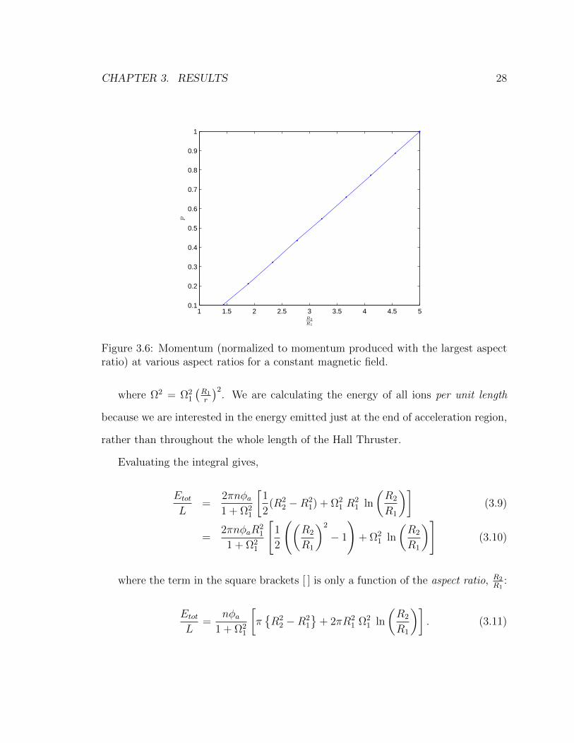
Figure 3.6: Momentum (normalized to momentum produced with the largest aspectratio) at various aspect ratios for a constant magnetic field.

where Ω2 = Ω21

(R1

r

)2. We are calculating the energy of all ions per unit length

because we are interested in the energy emitted just at the end of acceleration region,

rather than throughout the whole length of the Hall Thruster.

Evaluating the integral gives,

EtotL

=2πnφa1 + Ω2

1

[1

2(R2

2 −R21) + Ω2

1 R21 ln

(R2

R1

)](3.9)

=2πnφaR

21

1 + Ω21

[1

2

((R2

R1

)2

− 1

)+ Ω2

1 ln

(R2

R1

)](3.10)

where the term in the square brackets [ ] is only a function of the aspect ratio, R2

R1:

EtotL

=nφa

1 + Ω21

[πR2

2 −R21

+ 2πR2

1 Ω21 ln

(R2

R1

)]. (3.11)

CHAPTER 3. RESULTS 29

0.1 0.2 0.3 0.4 0.5 0.6 0.7 0.8 0.9 10.1

0.2

0.3

0.4

0.5

0.6

0.7

0.8

0.9

1

E

p

Figure 3.7: Momentum versus energy (each normalized to their greatest values) emit-ted by the system for a constant magnetic field.

The first term above in the square brackets is the cross-sectional area of the

thruster, and the second term depends on B1.

3.1.2 Momentum

The rate of input of ions into the acceleration region is N , where N is the number of

ions. If they are uniformly spread out over the cross-sectional area A = π(R22 − R2

1),

then the flux, i.e., the number per time per area, will be NA

and in each thin, cylindrical

shell with thickness dr at r, there will be NA

2πrdr ions per unit time.

These ions will reach the end of the acceleration region with energy eφmax(r), and

with a momentum P =√

2meφmax.

The total thrust, T , or momentum output per unit time will be:

CHAPTER 3. RESULTS 30

T =N

A2π√

2mq

∫ R2

R1

√φmax(r) rdr (3.12)

=N

A2π

√2mqφa1 + Ω2

1

∫ R2

R1

√r2 + Ω2

1 R21 dr, (3.13)

where A = πR21(α2 − 1), and α = R2

R1, the aspect ratio.

Executing and simplifying the integral above results in the following expression

for the approximate thrust assuming that φ is linear in z:

T =N√

2mqφaα2 − 1

[α

√α2 + Ω2

1

1 + Ω21

− 1 +Ω2

1√1 + Ω2

1

ln

α +

√α2 + Ω2

1

1 +√

1 + Ω21

]. (3.14)

3.2 Numerical Results

Figure 3.4 shows how the area of the annular region increases as a function of the

aspect ratio. As the area (A = π(R22 − R2

1)) of the annulus increases, the energy

and momentum of the system also increase. In Figures 3.5 through 3.7, we look

at a constant magnetic field value where various aspect ratios between a constant

inner radius and an increasing outer are used to find how the energy and momentum

change. As the aspect ratio increases, so does the system’s energy and momentum,

and as energy increases, momentum increases at an accelerating rate. In order to

maximize a Hall Thruster’s energy and momentum output, a designer may benefit

from a large ratio between inner and outer radii in the cylindrical acceleration region.

In order to conclude that Kornberg’s [11] one-dimensional conclusion holds true

CHAPTER 3. RESULTS 31

in two dimensions, we compared three different magnetic field structures: constant,

increasing, and decreasing, with all having the same average magnetic field value.

Figures 3.8 through 3.10 show these comparisons. In all three cases, the energy

and momentum output follow the same curve across increasing aspect ratios. These

results are similar enough to conclude that the shape of the magnetic field does not

have a significant effect on the energy and momentum output of a Hall Thruster

engine.

1 1.5 2 2.5 3 3.5 4 4.5 50.5

1

1.5

2

2.5

3

3.5

4x 10

−6

R2

R1

E

ConstantIncreasingDecreasing

Figure 3.8: Comparison of the energy emitted by the system at various aspect ratiosfor constant, increasing, and decreasing magnetic fields.

CHAPTER 3. RESULTS 32

1 1.5 2 2.5 3 3.5 4 4.5 50

0.2

0.4

0.6

0.8

1

1.2x 10

−5

R2

R1

p

ConstantIncreasingDecreasing

Figure 3.9: Comparison of the momentum of the system at various aspect ratios forconstant, increasing, and decreasing magnetic fields.

0.5 1 1.5 2 2.5 3 3.5 4

x 10−6

0

0.2

0.4

0.6

0.8

1

1.2x 10

−5

E

p

ConstantIncreasingDecreasing

Figure 3.10: Momentum versus energy emitted by the system at various aspect ratiosfor constant, increasing, and decreasing magnetic fields.

Chapter 4

Conclusion

A simplified one-dimensional model was expanded to two-dimensions in order to see

if the theory holds up that magnetic field shape does not play a strong roll in thrust

output. Solutions at the end of the acceleration chamber had varied ratios of inner to

outer radius. With the average magnetic field value held constant, momentum and

energy output were calculated with three magnetic field shape variations. The first

was constant, the next was a field that increased linearly from front to back of the

acceleration chamber, and the last decreased linearly.

Figures 3.8 through 3.10 show the patterns of energy and momentum of the parti-

cles expelled from the annular acceleration region created by these different magnetic

field structures do not show any appreciable differences. Thus, it can be concluded

that the shape of the magnetic field along the axis of a two-dimensional Hall Thruster

model has a negligible bearing on the amount h of thrust produced.

A possible subject of future interesting work would be to vary the constant, β, from

Choueiri’s energy relation, Equation (2.22). If the variation resulted in a significant

effect on electric potential profile, this could also affect the length of the acceleration

33

CHAPTER 4. CONCLUSION 34

region and in turn, the engine’s thrust.

Appendix A

Numerical Methods

The consequences of solving the two first order ordinary differential equations versus

one second order differential equation were explored using three different numerical

solvers. The three numerical methods used were fourth-order Runge Kutta (RK4),

Modified Midpoint and Adams-Bashforth-Moulton Four-step Explicit (ABM). All

solutions were very close to the solution using MATLAB’s built-in ODE45 solver.

Setting the solver at a fairly high tolerance (between 1 × 10−6 and 1 × 10−7) gives

more accurate solutions, and all seemed identical. One example is shown in Figure

A.1, where the two coupled first order ODEs, Equations (2.33) and (2.34) are solved

using the a fourth order Runge Kutta method. As the length of the acceleration region

(z) goes to zero, the potential (φ) will also drop to zero. For increasing magnetic field

values, the drop off will occur over a shorter distance. Plots of the differences between

each method (error) are shown in log-log scaling in Figures 2 through 6.

MATLAB’s built-in ODE45 function was considered good enough to use for the

analysis in this study.

35

APPENDIX A. NUMERICAL METHODS 36

Figure A.1: Two coupled first order ODEs calculating length of potential drop in theacceleration chamber solved with a fourth-order Runge Kutta method. Five differentf-values are plotted, each related to a different constant magnetic field.

Figure A.2: Log-log plot of error of the coupled first-order ODEs between RK4 andAMB methods.

APPENDIX A. NUMERICAL METHODS 37

Figure A.3: Log-log plot of error of the coupled first-order ODEs between RK4 andModified Midpoint methods.

Figure A.4: Log-log plot of error between the coupled first-order ODEs and the secondorder ODE both solved with RK4.

APPENDIX A. NUMERICAL METHODS 38

Figure A.5: Log-log plot of error between the coupled first-order ODEs solved withRK4 and the second order ODE solved with AMB.

Figure A.6: Log-log plot of error between the coupled first-order ODEs solved withRK4 and the second order ODE solved with Modified Midpoint.

Appendix A

MATLAB code

A.1 Define Differential Equation with Simple B

function phidot=oren(z,phi)

global Beta;

global f;

%B = 0.1;

p1=phi(1); %phi

p2=phi(2); %phi dot

phidot = [ p2;

(((p2ˆ2)/2)*(((1-p1)ˆ(-1))-Beta*((1-p1)ˆ(-1))-(3/2)*Beta*p1*

((1-p1)ˆ(-2))-Beta*((1-p1)ˆ(-1))-(2*(1+fˆ2))/(p2ˆ2)))/(Beta-1-

(Beta/2)*p1*((1-p1)ˆ(-1)))];

A.2 Define Differential Equation with Varying Bfunction phidot=orenuprightb(z,phi)

global Beta;

global f;

global zend;

global fz;

b = (2*f)/zend; %slope

%fz = -b*z+2*f;

39

APPENDIX A. MATLAB CODE 40

fz = b*z;

%%% sin/cos stuff

% fz=f*pi/2*sin(pi/zend*z);

%fz=f+f*cos(2*pi/zend*z);

% w=pi/zend;

% b=f*sqrt(2);

% fz=b*sin(w*z);

%B = 0.1;

p1=phi(1); %phi

p2=phi(2); %phi dot

phidot = [ p2;

(((p2ˆ2)/2)*(((1-p1)ˆ(-1))-Beta*((1-p1)ˆ(-1))-(3/2)*Beta*

p1*((1-p1)ˆ(-2))-Beta*((1-p1)ˆ(-1))-(2*(1+fzˆ2))/(p2ˆ2)))/

(Beta-1-(Beta/2)*p1*((1-p1)ˆ(-1)))];

A.3 Plot Resultsclose all

clear all

clc

%%%%%%%%%%%%%%%%%%%%%%%%%%%%%%%%%%%%%%%%%%%%%%%%%%%%%%%%%%%%%%%%%

%The aspect ratio of outer

%to inner radius is varied and the phi values at the end of the

%acceleration region are used to calculate energy and momentum as

%functions of aspect ratio.

%%%%%%%%%%%%%%%%%%%%%%%%%%%%%%%%%%%%%%%%%%%%%%%%%%%%%%%%%%%%%%%%%

dz = 1e-6; %step size

zspan = [0 1e-3]; %bounds of integration

phi0=[0 0.01]; %initial conditions

global Beta;

global f;

global R2;

global zend;

global fz;

Beta=.001;

options=odeset(’RelTol’,1e-9); %integration tolerence

li = [’-.’,’-’,’-’,’-’,’-’,’-’,’-’,’-’,’.’,’_’];

%li = [’r’,’b’,’k’,’g’,’y’,’m’,’b’,’k’,’g’,’y’];

APPENDIX A. MATLAB CODE 41

%li = [’y’,’r’,’y’,’y’,’y’,’y’,’y’,’y’,’y’,’c’];

R1 = 0.0005; %inner radius, fixed

% R2 = 1./linspace(1/R1,1/0.1,50); %varying outer radius INVERSELY GRIDDED

R2 = linspace(R1,0.05,50)

%R2 = 0.0015; %Make aspect ratio 3

%R2 = 0.00075; %Make aspect ratio 1.5

%R2 = 0.0006; %Make aspect ratio 1.2

aspectratio = R2/R1;

for j=2:2 %for each aspect ratio > 1

f0 = linspace(R1,R1*aspectratio(j),10); %make linear array of f’s

%f0 = linspace(R1,R1*aspectratio,6); %single aspect ratio

%f0 = [2000,1600,1400,1200,1000,800]; %choose my own f0s

zend=3e-3; %large first end of acc region

for i=1:length(f0) %for each magnetic field value throughout a different aspect ratio

f = 1/f0(i); %f’s are inverse of r’s

%f =f0(i);

ff(j-1,i) = f; %save f-values

if i == 1 %for the first one

[z,phi]=ode45(’oren’,[0 zend],phi0,options); %solve it

topphi = find(phi(:,1)>.9999, 1, ’first’); %find where the peak is almost = 1

zend = z(topphi); %set end of integration at phi = 1

phivalues(i) = phi(topphi,1); %all the phi values at the end of the acc region

else

[z,phi]=ode45(’oren’,[0 zend],phi0,options);

phivalues(i) = phi(end,1); %maxiumum phi for each aspect ratio (at end of acc reg)

%b = f/zend; %slope

%fz = -b*z+f;

%fz = b*z;

% figure(1)

% hold on

% plot(z,fz)

end

%str = num2str(aspectratio(j));

str = num2str(aspectratio); %single aspect ratio

figure(10+j)

hold on

plot(z/zend,phi(:,1),li(i+1)) %put dashed lines at R1 and R2

%plot(z/zend,phi(:,1),li(i)); %color the curves

xlabel(’$\barz$’,’interpreter’,’LaTeX’,’fontsize’,14)

ylabel(’$\bar\phi$’,’interpreter’,’LaTeX’)

% title([’Aspect Ratio = ’,num2str(aspectratio(j))])

%title([’Aspect Ratio = ’,num2str(aspectratio)]) %single aspect ratio

% hold on

% plot(z,phi(:,1));

end

%legend(’f = 2000’,’f = 1600’,’f = 1400’,’f = 1200’,’f = 1000’,’f = 800’);

APPENDIX A. MATLAB CODE 42

%legend(num2str(ff.’));

rr(j-1,:) = f0; %radius is inverse of magnetic field NEED TO MULT BY NUMBER OF PARTICLES, DIVIDE BY LENGTH?

Eintegrand(j-1,:) = phivalues.*rr(j-1,:).*2*pi; %inside of integal

EA = trapz(rr(j-1,:),Eintegrand(j-1,:)); %integrate between r1 and r2

A(j-1) = (pi*(rr(j-1,end)ˆ2-rr(j-1,1)ˆ2)); %toroid area

E(j-1) = EA/A(j-1); %divide by toroid area

m = 39.948*1.67262E-27; %mass of argon nucleus

pintegrand(j-1,:) = sqrt(phivalues.*2).*2.*pi.*rr(j-1,:);

p(j-1) = trapz(rr(j-1,:),pintegrand(j-1,:))./A(j-1);

end

% figure

% plot(aspectratio(2:end),E,’.-’)

% xlabel(’$\fracR_2R_1$’,’interpreter’,’LaTeX’);

% ylabel(’$E$’,’interpreter’,’LaTeX’);

%

% figure

% plot(aspectratio(2:end),p,’.-’)

% xlabel(’$\fracR_2R_1$’,’interpreter’,’LaTeX’);

% ylabel(’$p$’,’interpreter’,’LaTeX’);

%

% figure

% plot(E,p,’.-’)

% xlabel(’$E$’,’interpreter’,’LaTeX’);

% ylabel(’$p$’,’interpreter’,’LaTeX’);

%

% figure

% plot(aspectratio(2:end),A,’.-’)

% xlabel(’$\fracR_2R_1$’,’interpreter’,’LaTeX’);

% ylabel(’$A$’,’interpreter’,’LaTeX’);

Bibliography

[1] European Space Agency. Esa science and technology: Summary, smart-

1 propulsion. http://sci.esa.int/science-e/www/object/index.

cfm?fobjectid=31407&fbodylongid=850, 26 Jul 2006.

[2] Ahedo E., Martinez-Cerezo, P., Martinez-Sanchez, M. One-Dimensional Model

of the Plasma Flow in a Hall Thruster. Physics of Plasmas, vol. 8, no. 6:3058–

3068, 2001.

[3] Beal, B. E., Gallimore, A. D., Hargus, W. A. Preliminary Plume Characteriza-

tion of a Low-Power Hall Thruster Cluster. 38th Joint Propulsion Conference,

AIAA-2002-4251:5025–5033, July 7-10, 2002.

[4] E. Y. Choueiri. Fundamental difference between the two Hall thruster variants.

Physics of Plasmas, 8:5025–5033, November 2001.

[5] Clackamas Community College. Atomic size. http://dl.clackamas.cc.

or.us/ch104-07/atomic_size.htm, 2002.

[6] A. Fruchtman and N. Fisch. Modeling the Hall thruster. 34th

AIAA/ASME/SAE/ASEE Joint Propulsion Conference and Exhibit, July 1998.

43

BIBLIOGRAPHY 44

[7] Dan M. Goebel and Ira Katz. Fundamentals of Electric Propulsion: Ion and

Hall Thrusters. John Wiley and Sons, 2008.

[8] E. H. Hall. On the New Action of Magnetism on a Permanent Electric Current.

PhD thesis, The Johns Hopkins University, 1880.

[9] W. A. Hargus, Jr. Investigation of the plasma acceleration mechanism within a

coaxial hall thruster. PhD thesis, Stanford University, 2001.

[10] Richard Hofer. Development and characterization of high-efficiency, high-specific

impulse xenon Hall thrusters. PhD thesis, University of Michigan, 2004.

[11] Oren Kornberg. Investigation of Magnetic Field Profile Effects in Hall Thrusters .

M.S. thesis, Embry-Riddle Aeronautical University, 2007.

[12] Richard R. Hofer and Alec D. Gallimore. High-Specific Impulse Hall Thrusters,

Part 2: Efficiency Analysis. Journal Of Propulsion and Power, Vol. 22, No.

4:732–740, 2006.

[13] Ernst Stuhlinger. Ion Propulsion for Space Flight. McGraw-Hill, Inc., 1964.

[14] Igor T. Iakubov V. E. Fortov. The physics of non-ideal plasma. World Scientific,

2000.