THE EFFECT OF MATERIAL TRANSFER DEVICES ON HMA …

THE EFFECT OF MATERIAL TRANSFER DEVICES ON HMA MATERIAL UNIFORMITY

AND RIDE QUALITY

Final Report Project Number 930-471

By

Mary Stroup-Gardiner Frazier Parker

Kristy Burns Harris Barkley Williams

National Center for Asphalt Technology Auburn University Auburn, Alabama

Sponsored By

Alabama Department of Transportation Montgomery, Alabama

February 2004

DISCLAIMER THE CONTENTS OF THIS REPORT REFLECT THE VIEWS OF THE

AUTHORS WHO ARE RESPONSIBLE FOR THE FACTS AND ACCURACY OF THE DATA PRESENTED HEREIN. THE CONTENTS DO NOT

NECESSARILY REFLECT THE OFFICIAL VIEWS OR POLICIES OF THE ALABAMA DEPARTMENT OF TRANSPORTATION OR AUBURN

UNIVERSITY. THIS REPORT DOES NOT CONSITITUTE A STANDARD, SPECIFICATION, OR REGULATION.

ii

EXCUTIVE SUMMARY Alabama Department of Transportation (ALDOT) recently started to require

contractors to use a material transfer device (MTD) in the construction of hot mix

asphalt (HMA) pavements in order to minimize segregation. While some research has

been done that indicates that the use of a MTD will minimize both temperature and

gradation segregation of the mix components once the mix leaves the HMA plant, no

research has been done to evaluate the impact of a MTD on initial ride quality.

The objectives of this research were to document the influence of MTDs on

improving both mix uniformity (i.e., lack of segregation) and initial ride quality. The

scope of this project included the evaluation of four Alabama HMA projects

constructed during the 2001 and 2002 paving seasons. On three of the four projects,

both the binder and surface courses were evaluated. Areas of non-uniformity were

identified during construction using an infrared camera, with areas having a

temperature difference of more than 19oF being classified as non-uniform. Both ride

quality and uniformity after construction was completed was identified using data from

the Auburn University Roadware inertial profiler.

Results show that the inclusion of a MTD in the HMA paving train can

significantly reduce the non-uniformity of the mix as measured by either temperature

differences or texture variations. A MTD also results in significantly smoother HMA

pavements. These conclusions are based on the paving operations moving

continuously. Any stops, with or without a MTD, will result in both more non-uniform

(potentially segregated) areas and a rougher ride.

iii

TABLE OF CONTENTS

INTRODUCTION 1

BACKGROUND 2

Ride Quality 2

Uniformity of the HMA Mat 4

Material Transfer Devices 6

Blaw-Knox 6

Roadtec 7

RESEARCH PROGRAM 12

Objectives 12

Scope 12

PROJECT DESCRIPTIONS 13

Project 1 16

Project 1-1 17

Project 1-2 18

Project 2 18

Project 2-1 19

Project 2-2 19

Project 3 19

Project 3-1 20

Project 3-2 21

Project 4 21

DATA COLLECTION 22

HMA Mat Temperature Measurements 23

Texture and IRI Measurements 24

iv

RESULTS AND DISCUSSION 25

Data Organization and Preliminary Analysis 25

Influence of Material Transfer Devices on Initial Ride Quality 26

Statistical Analyses 36

Influence of Material Transfer Device on Ride Quality 37

Non-Uniformity in HMA Mat Temperatures

and Initial Ride Quality 38

Evaluation of Screed Extension Effect on Ride Quality 41

Influence of MTD on Surface Texture 43

Coefficient of Variation 45

Segregation Ratios 48

Non-Uniform Texture 49

Influence of Type of MTD on Texture Uniformity 53

CONCLUSIONS 55

REFERENCES 56

v

TABLE OF TABLES

Table 1. Machinery Variations Used for Trials. 6

Table 2. General Project Information. 14

Table 3. Mix Properties as Reported by Paving Contractors. 15

Table 4. Types of Aggregates Used as Reported by the Paving Contractors . 16

Table 5. Example of Temperature Anomaly and Smoothness Data. 26

Table 6. US 280 Phenix City Test Section Details (Project 1). 27

Table 7. US 80 Selma Test Section Details (Project 2). 28

Table 8. US 82 Reform Test Section Details (Project 3). 29

Table 9. I-85 Opelika Test Section Details (Project 4). 30

Table 10. Test Section Averages (IRI in inches/mile). 31

Table 11. Example of Paired t-test. 37

Table 12. F-test results. 38

Tble 13. t-test Results for Effect of MTD. 38

Table 14. Percentage of Test Sections with a Temperature Variation. 39

Table 15. Percentage of High IRI Sections with a Temperature Difference. 40

Table 16. Paired t-test Results for Effect of Temperature Variations. 41

Table 17. Paired t-test Results for Effect of Screed Extension. 42

Table 18. Display of All Data and Data from only Uniform Temperature Areas. 44

Table 19. Mean Texture Depth Limits. 47

Table 20. Segregation Limits set by NCHRP Report 441. 48

Table 21. Sample Texture Data from Project 3-1 without an MTD. 50

Table 22. Potential Maintenance Work. 51

vi

TABLE OF FIGURES

Figure 1. Dimensions of a Blaw-Knox MC-330 (Blaw-Knox, 2000). 8

Figure 2. Blaw-Know MC-330. 9

Figure 3. Dimensions of a Roadtec SB-2500B (Roadtec, 2002). 10

Figure 4. Roadtec SB-2500B- The red arrows show the path that the mix follow. 11

Figure 5. Alabama Map with the Locations of the Projects. 14

Figure 6. Project 1 Layout. 17

Figure 7. Layout of Project 2-1 the Binder Layer . 19

Figure 8. Layout of Project 3-1 the Binder Layer. 20

Figure 9. Layout of Project 3-2 the Surface Layer. 20

Figure 10. Layout of Project 4. 22

Figure 11. Infrared Camera Operator and Manual Distance Meter Operator. 23

Figure 12. Infrared Image of a Temperature Anomaly (20 minute paver stop). 24

Figure 13. Phenix City Frontage Road Baseline. 31

Figure 14. Selma Baseline Comparison. 34

Figure 15. Reform Baseline Comparison. 35

Figure 16. Average Mean Texture versus Average Standard Deviation. 45

Figure 17. Mean Texture Depth versus Coefficient of Variation. 46

Figure 18. Example of Mean Texture Limits from Project 4-1 without an MTD. 48

Figure 19. Bar Graph of the Number of Places with Possible Accelerated 52

Figure 20. Typical Non-Uniform Texture when a MTD is Not Used (Project 3-2). 54

Figure 21. Typical Texture Pattern When the Blaw-Knox MTD Used (Project 3-2). 54

vii

INTRODUCTION

Research has found that temperature differentials of more than 19°F (10°C)

indicated potentially segregated areas in the hot mix asphalt (HMA) mat. The higher this

temperature differential, the more likely segregation is present, which in turn leads to

differential material stiffness, density and life expectancy. The definition of segregation

includes both materials segregation and temperature segregation. It is likely that factors

such as the screed settling during a stop and the differential compaction of the HMA in

areas with different temperatures, either from material or temperature segregation, will lead

to anomalies in both texture and ride quality (Stroup-Gardiner and Brown 2000).

The transportation of mix from the plant to the job site is the first step in producing

high quality ride and pavement performance. Trucks should not be loaded with single

dumps from silos, as this contributes to segregation. Mix delivery must be planned

properly to have sufficient material for continuous movement of the paver. Also, trucks

should not bump the paver when dumping the mix into the hopper, which can lead to

localized rough ride. Trucks should not be allowed to run empty and a uniform head of

material with consistent temperature at the screed will ensure that the resistance on the

screed remains constant. All of these factors contribute to a smooth riding pavement with a

good life expectancy (Janoff 1997).

A method recently introduced to help achieve continuous movement of the paver

and a uniform flow of consistent mix is to include a material transfer device in the paving

train. The material transfer device eliminates stopping of the paver to connect with haul

trucks and provides some surge capacity to smooth out erratic, or non-uniform, mix

delivery. Also, the material transfer device or hopper insert remixes the asphalt concrete to

improve its temperature and gradation consistency as delivered to the paver. More

consistent mix should reduce segregation and temperature variation in the mat, which in

turn should increase smoothness.

1

BACKGROUND

The public’s satisfaction with a roadway is primarily based on the smoothness

(i.e., the absence of roughness) of the pavement. The first thing the average motorist

notices about a smooth pavement is there is less noise than a rough pavement. Also, after

a long trip, motorists realize that they are not as tired from the vibrations that would

result from a rough pavement. Smooth pavements that the public demands start with

smooth as-constructed pavement surfaces. Research has shown that initial smoothness is

important to both future smoothness and pavement life. The process of achieving quality

ride characteristics starts at the hot mix asphalt (HMA) plant and is a continuous,

uniform, and coordinated process through mat compaction. Consistent mix temperature

and continuous paving machine operation are critical parameters. The ideal situation is

that the mat, with uniform and consistent temperature, is laid down in a continuous

operation with minimal interruptions. Incentives through bonus payments to contractors

help produce smoother pavements have been estimated to increase pavement life by 10%

(Massucco 1999).

Ride Quality

A study of the relationship between initial smoothness and pavement life used 10

years of historical data from over 400 sections of roadway in Arizona and Pennsylvania

(Janoff 1991). The data included initial pavement smoothness, annual measurements of

smoothness, several forms of pavement distress, such as patching, cracking, rutting and

deflection, and annual maintenance costs. Through statistical analysis, it was shown that

the initial smoothness of a pavement is related to both long-term roughness and cracking.

Pavements that are initially smoother, even by a small amount, will have significantly

smaller rates of increase in roughness and cracking than pavements that are initially

rougher. Another effect determined in this study was that pavements that are initially

smoother have lower average annual maintenance costs. Average annual savings are

nearly $1200 per mile when initial smoothness, or initial Profile Index (PI), is reduced by

10 inches per mile (158 mm/km).

2

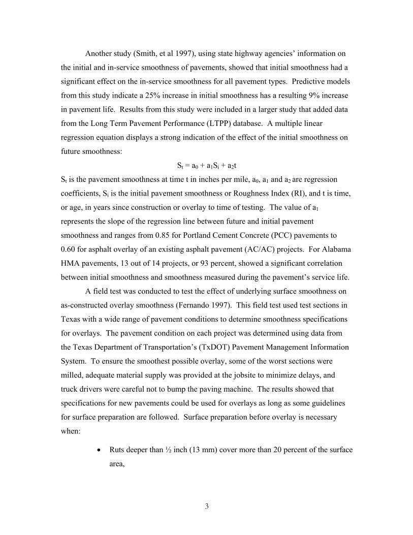
Another study (Smith, et al 1997), using state highway agencies’ information on

the initial and in-service smoothness of pavements, showed that initial smoothness had a

significant effect on the in-service smoothness for all pavement types. Predictive models

from this study indicate a 25% increase in initial smoothness has a resulting 9% increase

in pavement life. Results from this study were included in a larger study that added data

from the Long Term Pavement Performance (LTPP) database. A multiple linear

regression equation displays a strong indication of the effect of the initial smoothness on

future smoothness:

St = a0 + a1Si + a2t

St is the pavement smoothness at time t in inches per mile, a0, a1 and a2 are regression

coefficients, Si is the initial pavement smoothness or Roughness Index (RI), and t is time,

or age, in years since construction or overlay to time of testing. The value of a1

represents the slope of the regression line between future and initial pavement

smoothness and ranges from 0.85 for Portland Cement Concrete (PCC) pavements to

0.60 for asphalt overlay of an existing asphalt pavement (AC/AC) projects. For Alabama

HMA pavements, 13 out of 14 projects, or 93 percent, showed a significant correlation

between initial smoothness and smoothness measured during the pavement’s service life.

A field test was conducted to test the effect of underlying surface smoothness on

as-constructed overlay smoothness (Fernando 1997). This field test used test sections in

Texas with a wide range of pavement conditions to determine smoothness specifications

for overlays. The pavement condition on each project was determined using data from

the Texas Department of Transportation’s (TxDOT) Pavement Management Information

System. To ensure the smoothest possible overlay, some of the worst sections were

milled, adequate material supply was provided at the jobsite to minimize delays, and

truck drivers were careful not to bump the paving machine. The results showed that

specifications for new pavements could be used for overlays as long as some guidelines

for surface preparation are followed. Surface preparation before overlay is necessary

when:

• Ruts deeper than ½ inch (13 mm) cover more than 20 percent of the surface

area,

3

• Segments have more than one failure (failure not defined in study) per 0.6

mile (1 km), or

• More than 50% of the surface area is patched.

To determine factors that affect the ride quality of overlays, the Virginia

Department of Transportation conducted a study with roughness surveys of 2,650 lane-

miles of roadway. The study variables were limited to those that could be controlled by

the contractor, and a database was developed to help in the analysis. The factors that

were found to affect overlay smoothness were: (1) the roadway functional classification,

(2) the ride quality of the underlying pavement, and (3) a special provision for ensuring

smoothness. This special provision included using the International Roughness Index

(IRI) as the smoothness measurement and pay adjustments, incentive/disincentive, based

on the IRI. An overlay IRI of 60 to 70 inches per mile (950 to 1100 mm/km) is the range

for 100 percent pay, with IRI of over 100 inches per mile (1580 mm/km) requiring

corrective action. Lower overlay IRI values constitute the incentive part of the provision.

Functional classification is the grouping of highways by the character of service they

provide. The hierarchy of this functional system includes: principal arterials, minor

arterials, collectors, and local roads and streets. The effect of this factor is that the higher

classification roadways have smoother overlays. And with a smoother underlying

pavement, the results show that the overlay will be smoother. Finally, the addition of the

special provision with an incentive/disincentive clause motivates the contractor to

produce smoother pavements.

There were too few differences in overlay thickness to determine if this variable

affected ride quality. Mix type, an additional structural layer between base and overlay,

or multi-layer overlay, milling and the time of paving (night or day) did not affect overlay

smoothness (McGee 2000).

Uniformity of the HMA Mat

A method to help achieve continuous movement of the paver and a uniform flow of

consistent mix is to include a material transfer device (MTD) in the paving train. The

MTD eliminates stopping of the paver to connect with haul trucks and provides some surge

4

capacity to smooth out erratic, or non-uniform, mix delivery. Also, the MTD or a hopper

insert remixes the asphalt concrete to improve its temperature and gradation consistency as

delivered to the paver. Research on NCHRP Project 9-11 found that both temperature

differentials of more than 10EC (19E F) in hot mix asphalt concrete mats, and significant

changes in the surface texture are associated with segregated areas (Stroup-Gardiner and

Brown 2001). This research also showed the greater the non-uniformity (either

temperature or texture) the more likely segregation will occur followed by a noticeable

increase in pavement distresses in the segregated (non-uniform) areas. While it was also

hypothesized that areas with non-uniform properties would also have a localized rougher

ride, the original study did not include an evaluation of ride quality.

A Texas field test attempted to determine if several material transfer and remixing

devices could produce a smoother, less segregated pavement than conventional windrow

paving equipment (Asphalt Contractor 2000). The five consecutive days experiment used

a TxDOT type A mix, which was prone to segregation. Characteristics of a type A mix

are: a gradation curve with 60 percent of the aggregate 0.375 inches (10 mm) or larger,

100 percent passing 1.5 inches (38 mm) and very few fines. In this test, all material was

deposited in a windrow. The equipment used the first day, a BG-650 windrow elevator

and BG-260C asphalt paving machine (no remixing), was considered standard equipment

and used to compare the performance of other equipment. On the following days, four

different types of material transfer and remixing devices, identified in Table 1, were

added to the paving train. The results from density analyses indicated:

• Segregation by improper loading of delivery trucks or when dumped from the

trucks was not effectively reduced, nor could the material be remixed to

reduce segregation, by any of the equipment.

• Proper paving practices and well-trained crews have a major impact on quality

and can produce pavements that meet specifications using any method.

• There were no correlations between paving equipment, mat segregation and

mat density.

• Infrared cameras can be used to measure surface temperature variation

without correlation to density and smoothness.

5

Table 1. Machinery Variations Used for Trials. Day 1 BG-650 windrow elevator and BG-260C paver (control)

Day 2 Roadtec SB2500 material transfer vehicle and BG-260C paver with hopper insert (Roadtec picked up windrowed mix)

Day 3 Lincoln 880 windrow elevator and BG-260C paver with Lincoln pug mill hopper insert

Day 4 Cedarapids MS-2 windrow elevator and CT 461 remixer paver

Day 5 BG-650 windrow elevator / Blaw-Knox MC-330 mobile conveyor and BG-260C paver with Blaw-Knox pug mill hopper insert

Three types of segregation were found in the testing: cyclical end-of-load

segregation, random patch segregation and longitudinal stripe segregation. It was

discovered that, for three of five days, trucks were loaded with a single dump, and therefore

large amounts of coarse material were found at the end of each windrow dump causing

cyclical end-of-load segregation. Failure to maintain a constant level of mix in the hopper

caused coarse aggregate to roll toward the outside when filling and resulted in random

patch segregation. Stripe segregation was a result of improper adjustment of the paver

augers.

Material Transfer Devices

There are two commonly used material transfer devices by Alabama HMA

contractors: These are units manufactured by 1) Blaw-Knox, and 2) Roadtec.

Blaw-Knox

The haul trucks dump their load into the MC-330 Mobile Conveyer, which

has a 30-ton storage bin. The mix is then transported up a non-slip conveyer belt and is

dumped directly into the 14-ton hopper mounted on the front of the paver. The MC-330

does not have an internal auger that remixes the asphalt; therefore the only purpose of

this MTD is to move the mix to the paver enabling it to continuously pave without

stopping. Since the mix is not agitated by the MTD, this eliminates the need for a

ventilation system on the MTD, which can actually lower the temperature of the mix by

increasing the airflow over the mix. The paver-mounted surge bin has two transverse

mixing augers that re-mix and blend the asphalt before being placed on the road. The

MC-330 has few high-tech parts; therefore it infrequently breaks down and it is easier to

6

fix than the Roadtec SB-1500B if it does break down. Figure 1 shows the dimensions of

the MC-330 Mobile Conveyer and Figure 2 is an image of the MTD being utilized on a

paving job (Blaw-Knox 2000).

Roadtec

Haul trucks dump into the front of a SB-1500B and a converging auger, with the

help of vibrators, moves the mix up a conveyer into a 25-ton surge bin. Located inside

the surge bin is a triple-pitch-segmented auger that remixes the asphalt resulting in a mix

of even temperatures before another conveyer belt discharges the mix into the paver. A

15- to 20-ton hopper attaches to the front of the paver and enables the MTD to move

away from the paver with enough material to continue paving until the SB-2500B returns.

Another bonus feature on this model is a fume extraction system that removes fumes and

hot air to exhaust pipes and away from the paving crew. The dimensions of a SB-2500B

are displayed in Figure 3 and the utilization a Roadtec SB-2500B on project 4-1 is shown

in Figure 4 (Roadtec 2002).

7

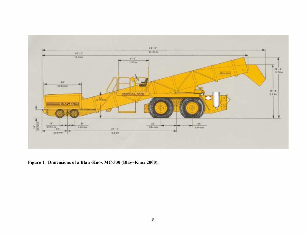
Figure 1. Dimensions of a Blaw-Knox MC-330 (Blaw-Knox 2000).

8

Haul Truck

Figure 2. Blaw-Know MC-330. (The red arrows sh

Augers remix HMA

ow the path that the mix follows).

9

Figure 3. Dimensions of a Roadtec SB-2500B (Roadtec 2002).

10

Figure 4. Roadtec SB-2500B- The red arrows show the p

Mix from haul truck

Augers remix HMA

ath that the mix follow.

11

RESEARCH PROGRAM

Objectives

The objectives of this research were to determine the effect of material transfer

devices on:

• Non-uniformity of HMA.

• Initial ride quality.

Localized areas of non-uniformity were identified during construction with infrared

thermography and changes in surface texture measured immediately after construction

was completed. Temperature differentials during construction were used to identify

localized areas of non-uniformity in the HMA mat. The longitudinal distance from the

start of the test section as well as the time each area was logged for correlation with IRI

values from the Roadware van. Changes in surface texture, also an indication of non-

uniformity in the HMA mat, were also evaluated as an indicator of areas of potentially

accelerated pavement distresses.

Scope

Projects were selected based on the contractors willing to pave both with

and without a material transfer device on existing ALDOT contracts. HMA mix

variables such as the maximum aggregate size and the binder type were included in the

study by evaluating different lifts on the same construction projects. Three Alabama

construction projects were evaluated with and without a material transfer device for both

the binder and surface mix lifts. While all of the mixes for these three projects met

Section 424 bituminous mixture ALDOT specifications, the binder lifts had a 1 inch

maximum aggregate size and used a PG 76-22 binder (ALDOT 2001). The surface mixes

had a maximum aggregate size of ½ to ¾ inch and used a PG 67-22 binder. A fourth

project was evaluated for only the binder lift. This mix was a stone matrix asphalt

(SMA). Designations for each mix for each project are used to indicate project and lift.

For example Project 1-2 indicates the second lift tested (i.e., surface mix) for project 1.

With the exception of Project 3-1, all of the areas tested were at least 3,000 feet

long. Project 3-1 lengths were shorter due to both equipment and weather problems; this

was also the only section that was paved during the winter season. The Project 3

12

contractor was also the only one that used other than a Roadtec MTD. Most of the

projects had paving lane widths of about 12 feet; Projects 2 and 3 widths were 14 and 16

feet, respectively. Project 1-2 was the only section that was placed over non-milled old

pavement.

An infrared camera used to monitor and mark potentially non-uniform

areas during construction. A walking distance wheel was used to determine the

longitudinal location of any areas with differences in the mat temperature of more than

19oF. Distances were entered into the field logs.

Once construction was completed and before the sections were opened to

traffic, Auburn University’s Roadware ARAN inertial profiler was used to determine IRI

in both wheel paths and the surface texture in the right wheel path. IRI values were

reported in inches/mile for every 26 feet of the test sections.

PROJECT DESCRIPTIONS

During this study, four separate HMA paving projects in Alabama were tested for

this project (Figure 5). Three of the four projects used the construction of both the binder

and surface mix for evaluating the influence of a MTD on mix uniformity (i.e., uniform

temperature, surface texture) and ride quality (i.e., IRI). Only the binder mix was tested

for Project 4 due to delays in construction.

13

3

4

2 1

Project Location with Corresponding Number Inside

Figure 5. Alabama Map with the Locations of the Projects.

Table 2 summarizes the lengths constructed with and without a material transfer

device (MTD) for each project, construction dates, type of surface preparation.

Table 2. General Project Information.

Project MTD used Date of Paving

Total Length (feet)

Lane Width (feet)

Temperature (oF)

high/low Weather MTD

Manufacture Surface

Preparation no 7/23/01 3139 11.5 None 1-1

Binder yes 7/25/01 2230 12.5 85 Clear,

humid (night)

Roadtec Milling & Chip Seal

no 8/15/01 3997 11 None 1-2 Surface yes 8/14/01 4100 11

85 Clear, humid (night)

Roadtec Patchwork &

Chip Seal

no 8/23/01 2950 12 None 2-1 Binder yes 8/23/01 2950 12

93 Clear, humid Roadtec

Milling

no 9/10/01 3140 14 None 2-2 Surface yes 9/10/01 2825 14


None

no 12/12/01 1813 16 None 3-1 Binder yes 12/12/01 1130 16

70 Clear, cloudy Blaw-Knox

Milling

no 5/23 and 5/24/02 4201 16 None 3-2 Surface yes 5/23/02 6022 16

75 Clear, dry Blaw-Knox

None

no 6/24/02 3877 12.5 None 4-1 Binder yes 6/24/02 2880 12.5


Milling Chip Seal

14

Table 3 summarizes a range of HMA information. All of the binder

course mixes were constructed using a polymer modified PG 76-22 binder and an

aggregate gradation with a 1 in. maximum size aggregate. Surface mixes used a PG 67-

22 with a maximum size aggregate of ½ to ¾ in; the gradations for the surface mixes

were finer than for the binder mixes. Project 4 used an SMA gradation, which makes it

the coarsest gradation evaluated for this project.

Table 3. Mix Properties as Reported by Paving Contractors. Project 1 Project 2 Project 3 Project 4

Binder Surface Binder Surface Binder Surface Binder

Binder Grade Type Mix PG 76-22

424 PG 67-22

424 PG 76-22

424 PG 67-22

424 PG 76-22

424 PG 67-22

424 PG 76-22

423 ESAL Category Range E Range C/D Range E Range E Range E Range C/D SMA Asphalt Content, % 3.9 5.7 4.1 4.6 4.75 5.5 5.5 AC Req'd/Ton 86 114 82 92 95 110 110 Max Specific Gravity 2.637 2.492 2.530 2.507 2.454 2.576 2.549 Unit Weight (lbs.)/ft3 157.7 148.9 151.2 149.7 146.5 153.8 152.3 VMA, % 13.0 16.3 13.7 14.0 13.8 15.0 17.0 TSR 0.90 0.86 0.86 0.90 0.85 0.88 0.86 Anti-strip additive, % --- --- --- 0.50 --- --- --- Effective AC Content, % 3.65 5.37 3.90 4.35 4.38 4.68 5.4 Dust/Asphalt Ratio 1.07 1.01 0.95 0.95 1.02 1.13 --- Coarse Agg. Angularity 100/100 100/100 98/96 98/96 99/98 100/100 100/100 Fine Agg. Angularity 49 46 45 45 45 45 47 Agg. Specific Gravity 2.792 2.693 2.683 2.675 2.608 2.765 2.784 Max. Aggregate size 1" 3/4" 1" 3/4" 1" 1/2" 1"

Sieve Size Cumulative Percent Passing, %

1” 100 100 100 100 100 100 100 3/4” 90 100 99 100 98 100 90 1/2” 75 95 88 96 89 100 74 3/8” 62 82 78 87 83 97 54 #4 43 64 55 61 64 72 28 #8 27 53 33.3 38.5 45 47 21 #16 20 42 22.1 25.3 34 34 17 #30 15 29 15.1 17.9 26 28 15 #50 13 15 7.8 9.3 15 14 11

#100 6 9 5 5.8 8 8 9 #200 3.9 5.4 3.7 4.1 4.5 5.3 8.0

---: no data available

15

Table 4 provides a general idea of the type and percentage of aggregate sources

used for each of the projects. Project 1 used various sources of limestone aggregates

while Project 3 used a combination of limestone and sandstone. Project 2 used a

combination of limestone and crushed gravel. All of the projects, except Project 1, used

some percentage of reclaimed asphalt pavement (RAP).

Table 4. Types of Aggregates Used as Reported by the Paving Contractors . Percent of Aggregate Stockpiles Used in Each Mix

Project 1 Project 2 Project 3 Project 4 Material

Binder Surface Binder Surface Binder Surface Binder Slag 25 #57 Limestone 33 30 # 67 Limestone 26 # 67 Sandstone 20 #78 Limestone 33 25 14 #78 Granite 15 44 ½” Crushed Gravel 24 #8910 Limestone 19 30 21 33 16 #8910 Sandstone 22 35 Coarse Sand 30 15 12 15 12 M10 Granite 14 10 Pea Gravel 14 14 Baghouse Fines 1 1 Fly Ash 5 Fibers 0.3 RAP 15 15 10 12 10

Project 1

Projects 1-1 and 1-2 were in an urban area of Phenix City in east Alabama on US

280 / 431 (Figure 6). This area is a four lane with a grass median and frontage roads on

both sides. The project involved rehabilitation of the mainline and frontage roads with

hot-mix asphalt (HMA) overlays. Because of traffic volumes, paving was done at night

from approximately 8 pm to 3 am. The project used a Roadtec 2500 material transfer

vehicle, and compaction was done with a vibratory breakdown roller factored by a steel

wheel finish roller. The haul time of the mix was approximately one hour.

16

Figure 6. Project 1 Layout.

SB

NB Grass Median

Frontage Rd-MTD

Frontage Rd-No MTD

N

Grass Median

Grass Median

Mainline-MTD

Mainline-No MTD

Project 1-1

Without MTD: Both nights an upper layer binder mix with a polymer modified

asphalt and a maximum aggregate size 1” was laid on top of freshly milled and chipped

sealed lanes. The mix designed for an ESAL range E was placed at a rate of 220 lb/yd2,

and was compacted using a vibratory breakdown roller with a steel finish. Traffic control

did not begin until 7 pm on the night of August 22, 2001 and the paving company

finished around 6 am on August 23 when all four lanes had to be reopened for traffic.

Paving started at the north end of the outside southbound lane without a MTD and

continued for 3,140 feet.

The second truck of the night had a spillage as it tried to lock up with the paver.

The paver was used to feather out the spill prior to paving. In the same night, the paver

had to stop an additional two times, besides the brief stops for haul trucks, to lower the

lights, once to go under traffic lights and a second time to go under a power line.

With MTD: Beginning at 1 am on August 25, a Roadtec MTD was used

to pave 2,230 feet of the inside southbound lane. Unlike the first night, a ski was used to

control the screed. Employing the MTD enabled the paver to maintain a continuous

forward movement. However, four stops were made by the paver while waiting for

additional haul trucks to arrive.

17

Project 1-2

About a month later the surface mix, project 1-2, was placed. This time the

frontage road on both sides of the mainline road were resurfaced. Before an overlay could

be placed, various areas had to be patched and the whole area was chip sealed. The

sections paved were the outside lanes of the west frontage road. At a rate of 165 lb/yd2, a

424 Superpave surface mix with a designed ESAL range of C/D and a maximum

aggregate size of ¾” was placed. The average width of the lanes was 11 feet, but

throughout both nights a screed was extended to accommodate numerous driveways and

parking areas. On the first night a Roadtec MTD was used to lay approximately 4000

feet. The next day construction continued from the joint and another 4100 feet of asphalt

was placed without the MTD.

Project 2

Both the binder and the surface layer (Project 2-1 and 2-2) were placed on a

stretch of US80 that is a four-lane highway divided by a grass median in Selma, Alabama

as shown in Figure 7. This area of highway was being repaved because of the extent of

rutting that had occurred due to the truck traffic in the area. The paving on this site

occurred from about 8 am to 4 pm on hot, sunny days in late August and early September

with highs up to 90oF. An unusual aspect to this site was that the asphalt plant was over

one hour away, which resulted in the plant mixing the asphalt at higher temperatures than

usual to compensate for the long haul distances. The temperature of the asphalt behind

the paver usually averaged between 320 and 340°F with a record high of 378°F. The

Selma project paving operation included a Blaw-Knox paver and a Roadtec 2500 material

transfer device. The mat compaction included two vibratory rollers and a steel wheel

finish roller.

18

Figure 7. Layout of Project 2-1 the Binder Layer .

EB

WB Grass Medium

MTD Binder Layer No MTD Binder Layer

N

No MTD Surface Layer MTD Surface Layer

Project 2-1

The binder test section was the 12-foot westbound inside lane. The 424 binder

mix, designed for ESAL range E, was placed at a rate of 225 lb/yd2 with a maximum

aggregate size of 1 inch. Before the binder layer could be laid, the area had to be milled.

After 3000 feet was laid without the employment of a MTD, another 3000 feet was paved

using a Roadtec MTD. Two vibratory rollers and a steel finish roller aided in the mat

compaction. Throughout the day the paver had to stop numerous times to wait for haul

trucks to arrive at the site.

Project 2-2

The surface test section was a 6000-foot continuous section with the latter 3000

feet utilizing the Roadtec MTD. Since a two-foot shoulder was included in this section of

paving, two extensions had to be utilized resulting in a 14-foot width. The test sections

were located on the inside westbound lane starting at the east end of the site. Designed

for ESAL range E and a maximum aggregate size of ¾ inch, the 424 mix was placed at a

rate of 165 lb/yd2.

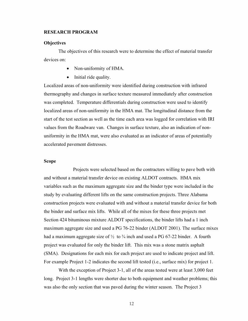
Project 3

Projects 3-1 and 3-2 are located on a four lane passing area with a grass

median on rural highway US82 outside of Reform, a small northwest Alabama town.

Figures 8 and 9 are layouts of the paved areas. A Blaw-Knox Mobile conveyor with a

19

pugmill hopper insert was the MTD used on the project, and two vibratory breakdown

rollers and one steel wheel finish roller performed the mat compaction. For both projects

3-1 and 3-2, a four-foot screed extension on the left and a two-foot one on the right

created a paving width of 16 feet.

Figure 8. Layout of Project 3-1 the Binder Layer.

EB

WB Grass Medium

MTD No MTD

N

Figure 9. Layout of Project 3-2 the Surface Layer.

EB

WB Grass Medium

MTD No MTD

N

Project 3-1

For the day the binder section was constructed, the weather was an above normal

December day with temperatures of approximately 50°F, a light breeze, and high

humidity. A light rain occurred for a few minutes while paving with the MTD. The

2,900-foot test section was located on the inside westbound lane. The first 1,800 feet was

paved without the MTD, and then the next 1,100 feet a Blaw-Knox MTD was added.

20

There were numerous stops being made by the paver, especially in the MTD section, due

to a lack of haul trucks. The binder mix designed for ESAL range E was a fine-grained

mix with a maximum aggregate size of 1 inch placed at a rate of 220 lbs/yd2.

Project 3-2

The finest mix of all the projects was incorporated with a maximum aggregate

size of ½ inch. The mix, designed for ESAL range E, was placed at a rate of 110 lbs/yd2.

Both days were sunny spring days with a temperature range of about 60 to 80°F. On the

first day of paving from about 1 pm to 5 pm approximately 6000 feet of asphalt was laid

in the inside eastbound lane using a Blaw-Knox MTD. In addition to the 6000 feet,

approximately another 650 feet was laid in the next hour without using the MTD in the

inside westbound lane. Starting at the joint from the night before, from 8 am to 10 am,

another 3,500 feet was laid without the MTD. Both days, trucks were lined up and only

occasional paver stops occurred towards the end of each section.

Project 4

Project 4-1 is located on I-85 outside of Auburn, Alabama and only a

binder layer was used for testing. The layout of this project is shown in Figure 10.

Paving took place on a hot humid day with temperatures reaching approximately 95°F.

The section was milled and chip sealed before the binder layer was placed. The SMA

mix was laid at a rate of 220 lbs/yd2 with a maximum aggregate size of 1 inch. One

vibratory roller and one steel wheel finish roller was used in the mat compaction of the

12.5 foot width lane. There was a wedge lock extension on each side with an additional

½ foot hydraulic extension on the left side.

21

Figure 10. Layout of Project 4.

NB

SB Grass Medium

MTD No MTD

N

The inside lane of the northbound highway was first paved without using a

MTD. On the 3,900-foot test section, the paver stopped briefly between each load and

once briefly to lower the truck bed to go under an overpass. At about 2 pm when the

paver turned the corner, the Roadtec MTD was used to pave a 2,900-foot section of the

inside southbound lane. About 700 feet after starting to pave with the MTD, the camera

battery went dead; therefore, only visual anomalies were documented after this point.

About 900 feet from the end of the project the paver slowed down to a crawl due to the

slowness of the arrival of the haul trucks; however, the paver never stopped.

DATA COLLECTION

Data collection involved several different processes. Notes of any construction

anomalies, such as trucks loaded with a single dump, were taken at the time of paving.

The temperature anomalies just behind the paver were noted using the infrared camera at

the time of paving. Both texture and IRI measurements were taken using the ARAN van

after completion of the test sections; the van was operated at about 25 mph for all projects

with the exception of Project 3.-2. Measurements on Project 3-2 (US 82, Reform, AL)

surface course were delayed approximately two months due to equipment problems with

the Roadware van at the time these sections were constructed. Testing was completed at

vehicle speeds of about 45 mph because of the live traffic at the time of testing.

22

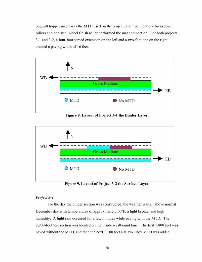
HMA Mat Temperature Measurements

The temperature differences, noted using an infrared camera, were differences in

the mat just behind the paver of over 20°F. The operator of the infrared camera sat in the

spare driver’s seat on the paver (Figure 11) and faced the screed, or hot mat. When a

temperature difference was seen, the operator took a picture of the anomaly with the

camera, which logs the pictures with the time, and then signaled the manual distance

meter operator. Figure 12 is an example that shows a temperature anomaly caused by a

paver stop. The manual distance meter operator noted the distance measurement, from

the start of paving, and the time the picture was taken. The time noted was used to

correlate the distance marks to the infrared pictures. In sections without the MTD, it was

common to see two cold spots, or one long cold spot, at the end of each truck of mix.

Figure 11. Infrared Camera Operator and Manual Distance Meter Operator.

23

60.0°C

160.0°C

60

80

100

120

140

160

SP01

SP02

AR01 AR02

Figure 12. Infrared Image of a Temperature Anomaly (20 minute paver stop).

Texture and IRI Measurements

Three runs (replicates) using the ARAN van were completed for each test section.

Both the average texture and IRI was computed for 15-foot long segments; texture was

obtained for only the right wheel path while the IRI was obtained in both the left and

right wheelpaths.

Most runs were taken at about 25 mph. The event key was used to mark the start,

the end and other important points in the section. These marks were used to correlate the

van distance measurements, which are called chainage in the ARAN system software, to

the manual distance meter.

24

RESULTS AND DISCUSSION

Data Organization and Preliminary Analysis

Each location and lift had test sections both without a material transfer device and

sections with remixing and a MTD. The infrared camera was used to detect mat

temperature and locations with temperature differences of 19°F were marked. The

marking of these differences included both the distance from the start of paving and the

time the anomaly was noted. The time is needed to correlate the distance to the images

since the infrared camera logs the images according to time. The ARAN van allowed

continuous measurement of IRI and distance from the start of paving. Using this van, the

data collection was set to give the IRI averages for each 15-foot section. Each 15-foot

length of the test section was divided into two categories: ones that had a temperature

difference of greater than 19°F and ones that had more uniform temperature throughout.

Table 5 is an example of the IRI data collected and illustrates how the van

measurements are correlated with the location of temperature anomalies. Column 1 is the

distance from the beginning of the test section to where a temperature anomaly in the mat

was noted. Columns 2 through 5and columns 6 through 9are distance, left wheelpath IRI,

right wheelpath IRI and average IRI for mat locations with uniform temperature and with

temperature anomalies, respectively.

From 3165 to 3195 feet, no temperature anomalies were observed and the IRI

values are recorded in columns 3 through 5. At a distance of 3201 feet, a temperature

anomaly was observed across the width of the mat and IRI values for the 3210 ft distance

are recorded in columns 7 through 9. The procedure followed was to match temperature

anomaly location with the closest 15 foot IRI section.

A long continuous temperature anomaly was noted on the right side of the mat

from a distance of 3266 feet to 3559 feet. Left wheelpath IRI corresponding to this

distance are recorded in column 3 but right wheelpath and average IRI are recorded in,

respectively, columns 8 and 9. Compilation and synthesis of data illustrated in Table 5

allows comparisons to determine differences in left and right wheelpath smoothness and

to determine effects of temperature anomalies on smoothness. Any blank cell denotes

that no entry is made in that category at that distance.

25

Table 5. Example of Temperature Anomaly and Smoothness Data.

Uniform Temperature Temperature Anomaly Distance to

Temp. Anomaly

Distance Left IRI

Right IRI

Avg. IRI Distance Left

IRI Right IRI

Avg. IRI

ft ft in/mile in/mile in/mile ft In/mile in/mile in/mile 3165 117 117 117 3180 236 282 259 3195 230 319 275

3201 3210 145 150 147 3225 159 89 124 3240 130 107 119 3255 95 46 70

3266* 3270 74 61 68 3285 87 44 65 3300 90 63 77 3315 127 84 105 3330 65 62 64 3345 39 60 50 3360 82 61 71

3375* 3375 83 48 66 3390 88 66 77 3405 69 86 78 3420 76 53 65 3435 65 40 52 3450 72 58 65 3465 115 68 92

3477* 3480 80 67 74 3495 64 49 56 3510 50 54 52 3525 72 76 74 3540 46 38 42 3555 79 58 69

3559* 3570 66 57 62 3585 50 56 53 3600 61 36 49 3615 35 47 41 * = anomaly continues to next section

Influence of Material Transfer Devices on Initial Ride Quality

Averages for the entire test section were obtained for each category, non-

uniform and uniform, and each of the three individual runs. These are tabulated in Tables

6 through 9 for Projects 1, 2, 3, and 4 (Phenix City, Selma, Reform, and Opelika)

26

respectively. Although averages for each run were computed from numerous IRI

measurements (1 per 15 feet), they were treated as an individual measurement in

statistical analyses, that is, the n value is equal to three.

Three runs were made with the ARAN van for each test section. The ARAN van

collects IRI in both right and left wheelpaths. Average IRI for each run were determined

for left, right and combined left and right wheelpaths. Averages for the three runs and

overall section averages are shown in Tables 6, 7, 8, and 9 for each of the four projects,

respectively.

Table 6. US 280 Phenix City Test Section Details (Project 1).

IRI in inches/mile without MTD with MTD

Section

Left IRI

Right IRI

Avg. IRI

Left IRI

Right IRI

Avg. IRI

Run 1 63 95 79 66 64 65 Run 2 60 87 74 66 65 65 Run 3 62 89 75 65 64 64

Total Run

Average 62 90 76 66 64 65 Run 1 58 90 74 66 63 65 Run 2 55 81 68 66 65 65 Run 3 57 83 70 65 64 64

Uniform


Project 1-1 (Mainline)

Non-Uniform


Total Run


Uniform


Project 1-2 (Frontage)

Non-Uniform

Average 81 86 84 98 146 122

27

Table 7. US 80 Selma Test Section Details (Project 2).

IRI in inches/mile

without MTD with MTD

Section

Left IRI

Right IRI

Avg. IRI

Left IRI

Right IRI

Avg. IRI

Run 1 66 66 66 55 58 56 Run 2 65 67 66 56 55 55 Run 3 65 68 66 55 55 55

Total Run


Uniform


Project 2-1 (Binder)

Non-Uniform


Total Run


Uniform


Non-Uniform

Average 105 95 100 80 67 73 Surface 101 88 94 69 55 62

Binder w MTD 84 52 68 91 59 75

Project 2-2 (Surface)

Difference Underlying

Binder IRIS-IRIB 16 36 26 -22 -4 -13

28

Table 8. US 82 Reform Test Section Details (Project 3).


Section

Left IRI

Right IRI

Avg. IRI

Left IRI

Right IRI

Avg. IRI

Run 1 69 68 68 65 52 58 Run 2 67 67 67 65 51 58 Run 3 69 68 69 63 53 58

Total Run


Uniform


Non-Uniform

Average 75 69 72 71 58 65 Run 1 47 61 54 Run 2 48 59 53 Run 3 48 58 53

Project 3-1 (Binder)

Total Run Eastbound

Outside Lane

Average 48 59 54 Run 1 48 52 50 41 40 41 Run 2 49 53 51 42 40 41 Run 3 48 52 50 41 41 41

Total Run


Uniform


Non-Uniform

Average 67 65 66 64 55 59 Surface 48 52 50 41 40 41

Binder w MTD

66 62 64 68 60 64

Project 3-2 (Surface)

Difference Underlying

Binder IRIS-IRIB -16 -9 -12 -26 -19 -22

29

Table 9. I-85 Opelika Test Section Details (Project 4).


Section

Left IRI

Right IRI

Avg. IRI

Left IRI

Right IRI

Avg. IRI

Run 1 73 65 69 68 57 63 Run 2 74 66 70 70 57 63 Run 3 73 66 70 67 58 63

Total Run


Uniform


(Project 4-1) Binder

Non-Uniform

Average 91 84 87 74 69 72

An examination of Tables 6 through 9 shows the surface mix test section on the

Project 1-2 (US 280 frontage road) was the only one where the smoothness without the

MTD was, unexpectedly, better than the smoothness with the MTD. A section of the

existing frontage road pavement, approximately 1800 feet, was tested prior to overlaying.

The average IRI of this section was 162 inches per mile, with some 15-foot section IRI

values as high as 1200 inches per mile as shown in Figure 13. This extremely rough

portion of the frontage road was part of the section placed with the material transfer

device, while the pavement in the section placed without the material transfer device was

much smoother. The highly variable roughness of the underlying pavement was thought

to be the reason for the unexpected surface IRI measurements, 69.36 inches per mile

without the MTD and 89.56 inches per mile with the MTD. The chip seal and the 165

pounds per square yard mix application rate were apparently not sufficient to eliminate

the effects of the underlying pavement roughness, which masked any beneficial effects of

the MTD.

Project 1-2 (Phenix City frontage road surface) data were not used in computing

averages shown in Table 10, nor for analyzing the influence of MTD’s, since it was the

only project that did not mill the old surface prior to paving. Averages in Table 10 were

computed by combining data from all other test sections.

30

0

500

1000

1500

0 0.5 1 1.5 2Distance (ft/1000)

IRI (

in/m

ile)

LIRI RIRI

Figure 13. Phenix City Frontage Road Baseline (Project 1-2).

Table 10. Test Section Averages (IRI in inches/mile).

Average of Average IRI, inches/mile With MTD 57.37 w/o MTD 70.81

Non-Uniform Areas 77.36 With MTD Uniform Areas 60.70 Non-Uniform Areas 81.59 w/o MTD Uniform Areas 63.67

Non-Uniform Areas 79.47 Uniform Areas 62.18

Extended Wheelpath IRI 70.55 Opposite Wheelpath IRI 62.01

Some additional testing was done on Projects 2-2 and 3-2 (Selma and Reform

surface) test sections. IRI measurements were made on the binder layer before paving to

give a baseline for evaluating smoothness improvements for the surface layer. It should

be noted that the binder and surface test sections were at different locations on each

project. However, the binder layers beneath surface test sections were placed with

MTD’s and should be comparable with corresponding binder test section layers. For

31

Project 2 (US 80 Selma), the average IRIs for binder below surface test sections were

somewhat larger (67.92 and 74.86 inches/mile) than the average IRI for binder with MTD

test section (55.64 inches/mile). For Project 3 (US 82 Reform), the same difference was

noted: the average IRIs for binder below the surface test sections were larger (64.34 and

63.58 inches per mile) than the average IRI for binder with the MTD test section (58.14

inches per mile). IRI for binder layers below surface test sections were not included in

calculations of test section averages in Table 10 or in subsequent statistical analyses.

Figures 14 and 15 show IRI of binder layers and corresponding IRI of overlying

surface layers. Differences between IRI measured on the surface and IRI measured on

the binder (IRIS – IRIB) are shown in Tables 7 and 8, and allow assessment of how much

improvement in smoothness is achieved with the surface layer. A comparison of values

with and without the MTD allows determination of how much more smoothness

improvement might be achieved with a MTD.

A close examination of Figure 14, for Project 2 (US 80 Selma), seems to indicate

surface IRI in the section without the MTD may indeed be larger than the binder IRI. IRI

differences in Table 7 confirm this observation. The positive (IRIS – IRIB) in the section

without the MTD indicates the surface layer is rougher than the binder layer. This is

unexpected and can only be explained by placement and/or compaction problems with

the surface layer. The negative (IRIS – IRIB) differences for the section with the MTD

show, as expected, the surface layer is smoother than the underlying binder layer.

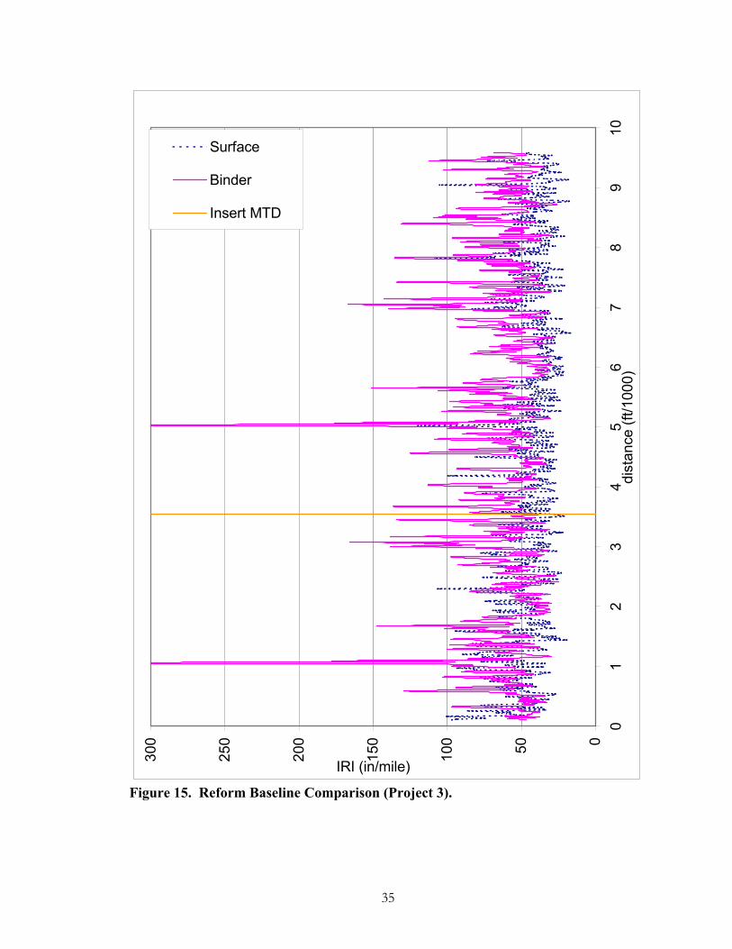
An examination of Figure 15, for Project 3 (US 82 Reform), shows the surface

layer is much smoother than the underlying binder. The IRI values in Table 8 confirm

that the surface layers (50.36 and 59.26 inches per mile) are smoother than the binder

layers (64.34 and 63.58 inches per mile). Also seen in Figure 15 is that large spikes in

the binder IRI are apparently smoothed out by the surface. For example at the distance of

1050 feet, the binder layer had an IRI of 326.98 inches per mile, while the overlying

surface has an IRI of 33.93 inches per mile. In Table 8, both average differences, IRIS –

IRIB, are negative, though the section with the MTD shows a much greater differential (-

22.34 inches per mile) than the section without the MTD (-12.22 inches per mile).

32

The presence of the MTD seems to make a significant improvement in the

smoothness of the overlying surface layer. Subsequent statistical analysis will indeed

show this to be the case.

Table 8 for Project 3 (US 82 Reform) contains several rows of data labeled

Binder, Total Run, and Eastbound Outside Lane. This layer was placed in the morning,

with the MTD, prior to placement of the binder test sections but no temperature

measurements were made. Binder test sections were placed on the adjacent westbound

inside lane beginning at about noon. This additional testing was done to record IRIs that

more accurately reflect the benefits of the MTD. In the binder test section in the

westbound lane placed with the MTD, mix delivery was so sporadic that continuous

paver movement was not possible and long stops were frequent. The total run averages

of IRI in Table 8 indicate the eastbound was somewhat smoother (53.53 inches/mile) than

the corresponding westbound (58.14 inches/mile). Data from the eastbound binder was

not used in computing section averages in Table 10, in analyzing the effects of the MTD

nor in analyzing the effects of temperature anomalies; none were measured. But, the data

was used in analyzing the effects of screed extensions.

33

01

23

45

6050100

150

200

250

300

IRI (in/mile)

dist

ance

(ft/1

000)

Surface

Binder

Insert MTD

Figure 14. Selma Baseline Comparison (Project 2).

34

01

23

45

67

89

10050100

150

200

250

300

IRI (in/mile)

dist

ance

(ft/1

000)

Surface

Binder

Insert MTD

Figure 15. Reform Baseline Comparison (Project 3).

35

Averages for all sections in Table 10 demonstrate the effects of (1) the MTD, (2)

temperature anomalies (uniform and non-uniform) and (3) screed extensions (extended

and opposite wheelpath). Comparisons in rows 1 and 2 show that average IRI with the

MTD are smaller than IRIs without the MTD. Comparisons in rows 3 through 8 show

that average IRIs where temperature anomalies were observed (non-uniform areas) are

larger than IRIs where mat temperatures were more uniform. The comparison in rows 9

and 10 shows that IRI in wheelpaths on the side with a screed extension or with the larger

screed extension are greater than IRI in wheelpaths on the side without a screed extension

or with the smaller screed extension. The statistical significance of differences will be

examined in the following section.

Statistical Analyses

Since analyses will be testing differences between averages of the three runs with

different treatments, such as left to right wheelpath and mark to no mark comparisons, the

t-test for means was chosen for the analysis. The t-test was conducted using the software

in the Analysis Toolpak of Microsoft Excel. This same test was used for comparisons

across all sites to compare the computed t statistic with the t critical value for a

confidence level of 95%. Means were considered to be significantly different if the

absolute value of the computed t statistic was greater than the absolute value of t critical.

The comparison to determine the effect of the material transfer devices used the t-

test assuming equal variance or the t-test assuming unequal variance. Equality of

variances was tested using the one-tailed F test with a confidence level of 95%.

The two tailed, paired t-test was used for the comparison between wheelpaths

(effects of screed extension) and the comparison between temperature differences since

the treatments to be compared used the same data source, i.e. IRI measurements on the

same mat. Thus the samples were not truly independent of one another. The degrees of

freedom for each comparison were the number of values in a category minus one.

To illustrate the application of the paired two-sample t-test, the US 280 Left and

Right IRI frontage road surface measurements with the MTD will be used. In this

section, the right wheelpath is the extended wheelpath. Using the data found in Table 6,

the hypothesis test of equality of mean IRI values, with and without the MTD, is

36

presented in Table 11. The analysis concludes that the IRI in the wheel path on the side

with the screed extension (right) is significantly larger than the IRI in the opposite (left)

wheelpath.

Table 11. Example of Paired t-test.

u1 = Population mean IRI without MTD u2 = Population mean IRI with MTD

Hypothesis H0 = u1 = u2 H1 = u1 ≠ u2

Extended (right) IRI w/o MTD (inches/mile)

Opposite (left) IRI w MTD (inches/mile)

di = difference (inches/mile)

100.32 76.74 23.58 101.97 75.97 26.00 105.65 76.73 28.92

Mean d = (∑di)/(n) = 78.50 / 3 = 26.167 inches/mile

sd = √ (∑(di – mean d)2/(n-1)) = 7.1497 inches/mile

Test Statistic: t = mean d*√n / sd = 16.9 Two tailed t critical: tcr = 4.30

Since t > tcr ⇒ Reject H0 ∴Difference in means is significant

Influence of Material Transfer Device on Ride Quality

An F-test for variances was used to evaluate the uniformity of the IRI

measurements within each wheel path and test section. The results of this analysis are

shown in Table 12. Since each run has the same beginning and ending, variance is a

result of different longitudinal paths being tracked with each run. The results show that,

for most sections, the variance is smaller for sections with the MTD. This shows that

there is less transverse variation in the mat when a material transfer device is present.

37

Table 12. F-test results.

Section with MTD Variance

w/o MTD Variance

F stat F critical Equal Variances?

US 280 Mainline 0.16 8.09 51.28 19.0 No Binder 0.04 0.39 0.102 0.053 No US80 Surface 4.36 1.90 0.435 0.053 Binder 0.08 0.59 7.08 19.0 Yes US 82 Surface 0.004 0.038 9.35 19.0 Yes

I 85 Binder 0.09 0.164 0.548 0.053 No

No

The t-test assuming unequal variances was used to determine if the variance in

ride quality (i.e., IRI) within a test section was influenced by the use of a MTD. The

complete results of the evaluation of the influence of material transfer devices in Table 13

show that, for every comparison, the addition of a MTD into the paving train resulted in a

significantly smoother pavement. For each mix type at each project, average IRI values

were from the three runs of the ARAN van.

Table 13. t-test Results for Effect of MTD.

Section with MTD AIRI

w/o MTD AIRI

t stat t critical Significantly Different ?

US 280 Mainline 65 76 6.73 4.30 Yes Binder 56 66 27.67 4.30 Yes US80 Surface 62 94 22.17 3.18 Yes Binder 58 68 20.82 2.78 Yes US 82 Surface 41 50 79.65 2.78 Yes

I 85 Binder 63 70 34.93 4.30 Yes

Non-Uniformity in HMA Mat Temperatures and Initial Ride Quality

The analysis in the previous section showed the MTD has a significant beneficial

effect on pavement smoothness. It is speculated that one of the primary reasons for this

is the MTD provides more uniform temperature mix at a more uniform rate which results

in more uniform mat temperature. Mat temperature measurements with the infrared

camera will be used to investigate mat temperature uniformity.

The 15-foot sections with a temperature difference of greater than 19°F were

separated from the sections with uniform temperatures. These 15-foot sections

correspond to sections where IRI values were computed. The total number of sections in

38

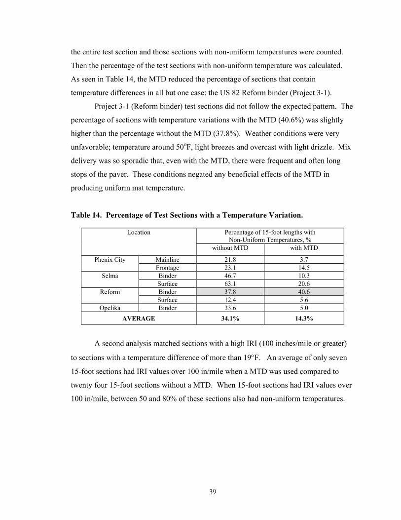
the entire test section and those sections with non-uniform temperatures were counted.

Then the percentage of the test sections with non-uniform temperature was calculated.

As seen in Table 14, the MTD reduced the percentage of sections that contain

temperature differences in all but one case: the US 82 Reform binder (Project 3-1).

Project 3-1 (Reform binder) test sections did not follow the expected pattern. The

percentage of sections with temperature variations with the MTD (40.6%) was slightly

higher than the percentage without the MTD (37.8%). Weather conditions were very

unfavorable; temperature around 50oF, light breezes and overcast with light drizzle. Mix

delivery was so sporadic that, even with the MTD, there were frequent and often long

stops of the paver. These conditions negated any beneficial effects of the MTD in

producing uniform mat temperature.

Table 14. Percentage of Test Sections with a Temperature Variation.

Percentage of 15-foot lengths with Non-Uniform Temperatures, %

Location


Mainline 21.8 3.7 Phenix City Frontage 23.1 14.5 Binder 46.7 10.3 Selma Surface 63.1 20.6 Binder 37.8 40.6 Reform Surface 12.4 5.6

Opelika Binder 33.6 5.0 AVERAGE 34.1% 14.3%

A second analysis matched sections with a high IRI (100 inches/mile or greater)

to sections with a temperature difference of more than 19°F. An average of only seven

15-foot sections had IRI values over 100 in/mile when a MTD was used compared to

twenty four 15-foot sections without a MTD. When 15-foot sections had IRI values over

100 in/mile, between 50 and 80% of these sections also had non-uniform temperatures.

39

Table 15. Percentage of High IRI Sections with a Temperature Difference. Number of 15-foot Sections with Non-Uniform Temperatures out of

Number of 15-foot Sections with IRI > 100 in/mile


Location

No. Non-Uniform to No. with IRI> 100 Percent (%)

No. Non-Uniform to No. with IRI>

100 Percent (%)

Phenix City

Main 22 out of 31 71.0 0 out of 9 0.0

Binder 15 out of 17 88.2 10 out of13 76.9 Selma

Surface 61 out of 63 96.8 5 out of 7 71.4

Binder 10 out of13 76.9 1 out of 2 50.0 Reform

Surface 2 out of 3 66.7 1 out of 1 100

Opelika Binder 19 out of19 100 2 out of 9 22.2

AVERAGE 20 out of 24 83.27 3.7 out of 7 53.42

A final analysis compared IRI from 15-foot sections with non-uniform

temperatures to those with uniform temperatures. A paired t-test was used to determine if

IRI values were statistically lower when using a MTD. Table 16 shows that in all but one

case (Project 1-1), the use of a MTD significantly reduces the IRI. This table also shows

that non-uniform temperature areas of the HMA pavement have significantly higher IRI

than when paving operations place mixtures with a uniform temperature.

40

Table 16. Paired t-test Results for Effect of Temperature Variations.

Section IRI in Non-Uniform Areas

in /mile

IRI in Uniform Areas in/mile

t stat t critical Significantly Different?

MTD 61 65 2.70 4.30 No Main No MTD 95 71 32.54 4.30 Yes MTD 122 84 45.06 4.30 Yes

US280

Front No MTD 84 65 57.48 4.30 Yes MTD 82 53 25.08 4.30 Yes Binder No MTD 74 59 13.09 4.30 Yes MTD 73 59 7.91 4.30 Yes

US80

Surface No MTD 100 85 15.64 4.30 Yes MTD 65 54 8.74 4.30 Yes Binder No MTD 72 66 27.45 4.30 Yes MTD 59 40 891.5 4.30 Yes

US 82

Surface No MTD 66 48 13.60 4.30 Yes MTD 72 62 5.87 4.30 Yes I 85 Binder No MTD 87 61 26.55 4.30 Yes

MTD 77 61 77 61 Yes No MTD 82 64 82 64 Yes

Overall Comparison 80 62 79 62 Yes

Evaluation of Screed Extension Effect on Ride Quality

Although not related to the use of an MTD, consistent effects of screed extensions

were noted when analyzing smoothness data. Consistent differences were noted between

IRI in wheelpaths on the side where screeds were extended or where screed extensions

were the largest and IRI in the opposite wheelpaths. Screed extensions are most often

used and/or larger toward the outside or shoulder. Correspondence of direction and/or

magnitude of screed extension and left and right wheel path IRI measurements will

depend on the lane being paved. Most screeds today are ten feet wide, and since most

paving lane widths are wider than ten feet, screed extensions are common and, therefore,

differences in wheelpath roughness will likely be common.

The t-test analysis, to determine the effect of screed extension is summarized in

Table 17. In every case except Project 2-1 (US 80 Selma binder) sections and Project 3-2

(US 82 Reform surface) without the MTD, the wheelpath with the extension had a higher

IRI than the other wheelpath. However, in these three cases the differences are not

significant.

41

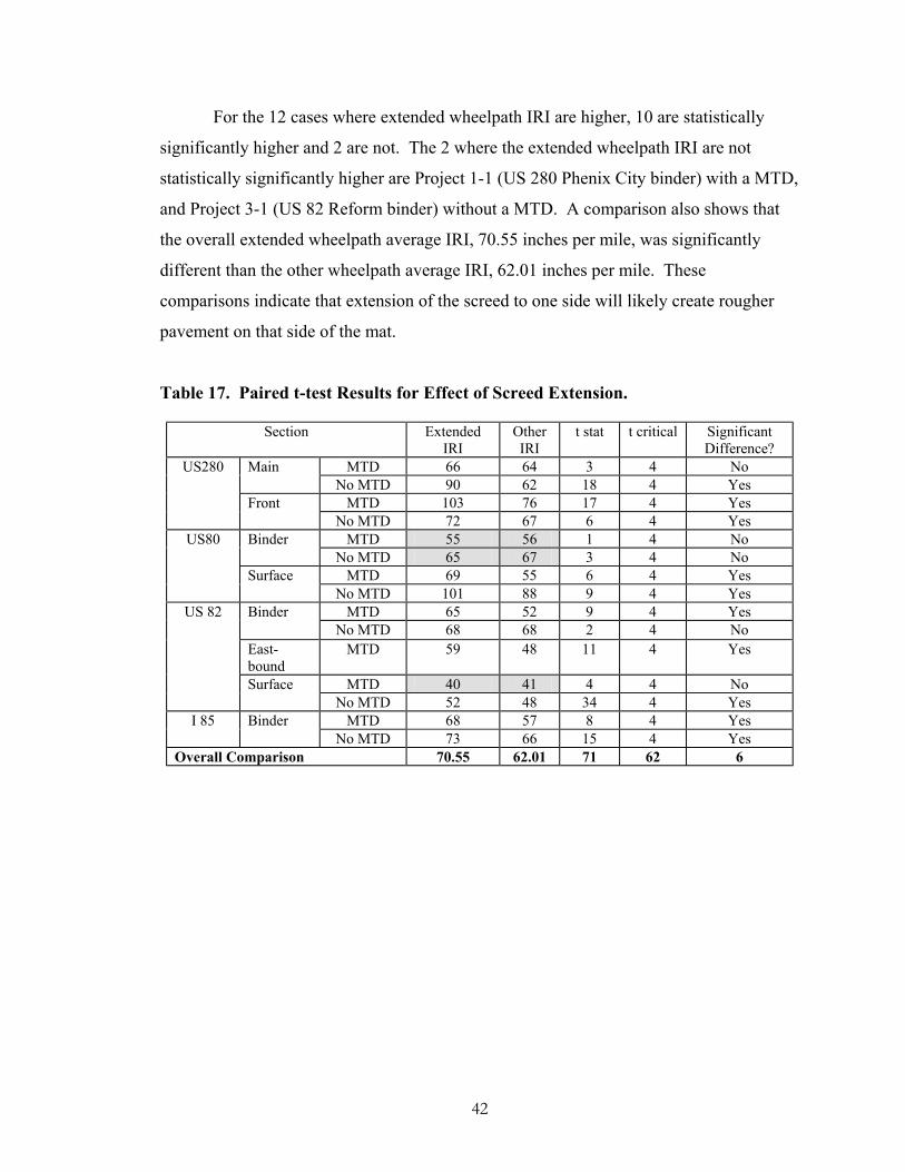
For the 12 cases where extended wheelpath IRI are higher, 10 are statistically

significantly higher and 2 are not. The 2 where the extended wheelpath IRI are not

statistically significantly higher are Project 1-1 (US 280 Phenix City binder) with a MTD,

and Project 3-1 (US 82 Reform binder) without a MTD. A comparison also shows that

the overall extended wheelpath average IRI, 70.55 inches per mile, was significantly

different than the other wheelpath average IRI, 62.01 inches per mile. These

comparisons indicate that extension of the screed to one side will likely create rougher

pavement on that side of the mat.

Table 17. Paired t-test Results for Effect of Screed Extension.

Section Extended IRI

Other IRI

t stat t critical Significant Difference?

MTD 66 64 3 4 No Main No MTD 90 62 18 4 Yes

MTD 103 76 17 4 Yes

US280

Front No MTD 72 67 6 4 Yes

MTD 55 56 1 4 No Binder No MTD 65 67 3 4 No

MTD 69 55 6 4 Yes

US80

Surface No MTD 101 88 9 4 Yes

MTD 65 52 9 4 Yes Binder No MTD 68 68 2 4 No

East- bound

MTD 59 48 11 4 Yes

MTD 40 41 4 4 No

US 82

Surface No MTD 52 48 34 4 Yes

MTD 68 57 8 4 Yes I 85 Binder No MTD 73 66 15 4 Yes

Overall Comparison 70.55 62.01 71 62 6

42

Influence of MTD on Surface Texture

The mean texture depth (in millimeters) average, variance, standard

deviation, and coefficient of variation are documented in Table 18. Statistics for uniform

temperature areas are also shown in Table 18.

The average mean texture depth, variance, standard deviation, and

coefficient of variation were also calculated for each run separately and the data are

documented in Table 18.

Project 3 had various problems that occurred on the site including bad weather,

length of the project, lack of haul trucks, a four-foot screed extension, and a power

system failure in the van at the end of testing. Therefore, these sections were eliminated

from the texture analysis.

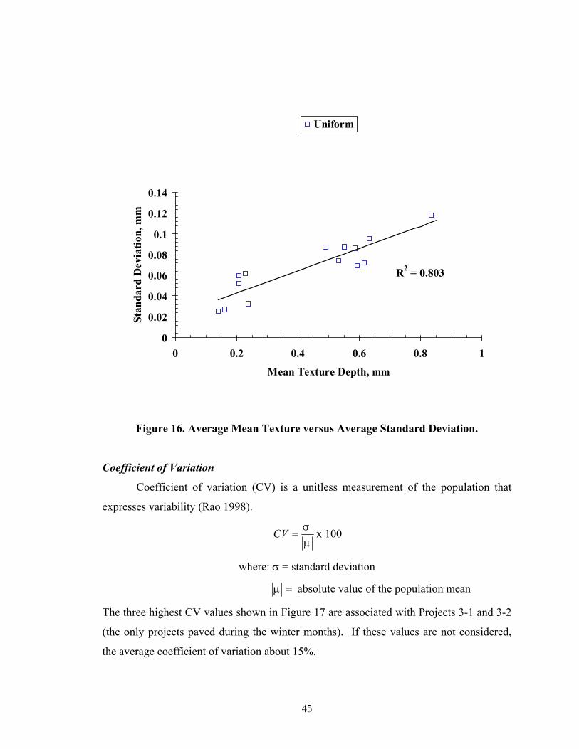
Within-Laboratory Precision

Figure 16 shows the standard deviation is dependent upon the mean texture.

Therefore, the coefficient of variation (CV) was evaluated as the most appropriate

statistic to represent variability.

43

Table 18. Display of All Data and Data from only Uniform Temperature Areas.

All Data Uniform Temperature Areas

Project Shuttle Buggy

Total Chainage

(feet)

Total Number of Stops

Average Texture

(mm)

Number of Data

Points (n) variance

(s2)

Standard Deviation

(mm)

Coefficient of Variation

(%)

Average Texture

(mm)

Number of Data

Points (n) variance

(s2)

Standard Deviation

(mm)


(%) No 3139 5 0.853 512 0.0149 0.1222 14.33 0.836 449 0.0138 0.1176 14.071-1

binder yes 2230 4 0.633 351 0.0091 0.0954 15.07 0.633 346 0.0091 0.0952 15.04No 3997 11 0.163 643 0.0007 0.0274 16.81 0.162 558 0.0008 0.0274 16.911-2

surface yes 4100 7 0.140 577 0.0007 0.0255 18.21 0.140 560 0.0007 0.0255 18.21No 2950 12 0.600 473 0.0053 0.0729 12.15 0.593 392 0.0048 0.0693 11.692-1

binder yes 2950 4 0.622 470 0.0057 0.0755 12.14 0.617 423 0.0052 0.0722 11.70No 3140 12 0.506 504 0.0096 0.0978 19.33 0.490 410 0.0076 0.0870 17.762-2

surface Yes 2825 2 0.533 374 0.0056 0.0746 14.00 0.533 350 0.0055 0.0739 13.86No 1813 14 0.233 295 0.0040 0.0636 27.30 0.229 225 0.0038 0.0619 27.03 3-1

binder Yes 1130 3 0.216 179 0.0047 0.0688 31.85 0.207 127 0.0036 0.0598 28.89 3-2 No 4201 17 0.216 672 0.0027 0.0517 23.94 0.208 552 0.0027 0.0521 25.05

surface Yes 6022 6 0.239 963 0.0011 0.0326 13.64 0.238 880 0.0011 0.0325 13.66No 3877 30 0.618 621 0.0098 0.0991 16.04 0.586 420 0.0074 0.0859 14.664-1

binder Yes 2880 1 0.560 463 0.0092 0.0961 17.16 0.550 429 0.0077 0.0875 15.91 average CV = 14.73

Note: Shaded areas not included in averages or other analysis

44

R2 = 0.803

0

0.02

0.04

0.06

0.08

0.1

0.12

0.14

0 0.2 0.4 0.6 0.8 1

Mean Texture Depth, mm

Stan

dard

Dev

iatio

n, m

mUniform

Figure 16. Average Mean Texture versus Average Standard Deviation.


Coefficient of variation (CV) is a unitless measurement of the population that

expresses variability (Rao 1998).

µσ

=CV x 100

where: σ = standard deviation

=µ absolute value of the population mean

The three highest CV values shown in Figure 17 are associated with Projects 3-1 and 3-2

(the only projects paved during the winter months). If these values are not considered,

the average coefficient of variation about 15%.

45

0

5

10

15

20

25

30

35

0 0.2 0.4 0.6 0.8 1

Mean Texture Depth, mm

Coe

ffici

ent o

f Var

iatio

n, %

Problems Removed

Figure 17. Mean Texture Depth versus Coefficient of Variation.

From the data of problems removed with an MTD without Project 3-1 documented on

Table 18, an average coefficient of variation, 14.6%, was calculated. From the slope of

Figure 18 the coefficient of variation should be 14.1 % and is probably different from the

calculated average because of rounding errors; therefore, for simplicity 15% was used in

the calculations. A new standard deviation was then found for each site separately by

rearranging the formula for the coefficient of variation and solving for the standard

deviation.

µσ *CV=

Using the calculated standard deviation, maximum and minimum limits were set for each

site separately according to the formulas displayed below. Anything above or below

these limits are areas predicted to have a significant amount of gradation segregation and

possibly need maintenance work before the end of its designed life cycle. Areas with

statistically higher texture will likely show accelerated pavement distresses while areas

46

with statistically lower texture will possibly have safety problems such as slick surfaces.

Using ± two standard deviations ensures that 95% of the data will be within the mean

maximum and minimum limits.

Maximum Mean Texture Depth = Average Mean Texture Depth + 2 * Calculated

Standard Deviation

Minimum Mean Texture Depth = Average Mean Texture Depth - 2 * Calculated

Standard Deviation

Table 19 displays limits for each mix. The limits are also displayed as lines on the graph

of chainage versus average texture depth in Figure 20 for project 4-1 without an MTD.

Six out of the eight paver stops resulted in non-uniform areas that will most likely result

in premature pavement distress. All eight stops resulted in mean texture depths above

one standard deviation. On these figures, paver stops are indicated by a “PS”.

Table 19. Mean Texture Depth Limits.


Average Texture (mm)

STD Dev from CV

(mm) Ave Texture +/- one

STD Dev (mm) Ave Texture +/- two

STD Dev (mm) No 0.836 0.125 0.711 – 0.961 0.585 - 1.087

1-1 binder Yes 0.633 0.095 0.538 – 0.728 0.443 - 0.823 No 0.162 0.024 0.138 – 0.186 0.113 - 0.211

1-2 surface Yes 0.140 0.021 0.119 – 0.161 0.098 - 0.182 No 0.593 0.089 0.504 – 0.682 0.415 - 0.771

2-1 binder Yes 0.617 0.093 0.524 – 0.710 0.432 - 0.802 No 0.490 0.074 0.417 – 0.564 0.343 - 0.637

2-2 surface Yes 0.533 0.080 0.453 – 0.613 0.373 - 0.693 No 0.229 0.034 0.195 – 0.263 0.160 - 0.298

3-1 binder Yes 0.207 0.031 0.176 – 0.238 0.145 - 0.269 No 0.208 0.031 0.177 – 0.239 0.146 - 0.270

3-2 surface Yes 0.238 0.036 0.202 – 0.274 0.167 - 0.309 No 0.586 0.088 0.498 – 0.674 0.410 - 0.762

4-1 binder Yes 0.550 0.083 0.468 – 0.633 0.385 - 0.715

47

0

0.25

0.5

0.75

1

1.25

1.5

0 250 500 750 1000

Chainage, feet

Aver

age T

extu

re D

epth

, mm

PSPSPSPSPSPSPSPS

+2 STD Dev +1 STD Dev Avg. Texture -1 STD Dev

-2 STD Dev

PS = Paver Stop Figure 18. Example of Mean Texture Limits from Project 4-1 without an MTD.

Segregation Ratios

Even though mean texture depth is mix dependent, the ratio of the texture

depth for a point to the average mean texture depth of the section will indicate the level

of segregation according to NCHRP Report 441, “Segregation in Hot-Mix Asphalt

Pavements” (Stroup-Gardiner, 2000). The ratios for low, medium, and high segregation

are displayed in Table 20 with the respective standard deviations. For data lower than the

mean texture depth a low ratio limit of 0.75 is set which corresponds to possible areas of

loss of skid resistance in the pavement mat.

Table 20. Segregation Limits set by NCHRP Report 441. Amount of segregation Low medium high ratio limits 1.16 - 1.56 1.57 - 2.09 >2.09

standard deviation 0.15 0.22 0.42

From the data gathered the ratio of the texture depth for above/below one standard

deviation to the average mean texture results in ratios of 0.85-1.15 and for two standards

deviations is 0.70-1.30. Therefore, the area below two standard deviations with the ratio

of 0.70 is similar to the ratio of 0.75 found in Report 441. A ratio of 1.30 is about in the

48

middle of low segregation range from Report 441 and is the point considered to need

maintenance in this current research study.

Non-Uniform Texture

Potential maintenance work will probably need to occur when the data is above

and below the texture limits already established in Table 20. Table 21 displays sample

texture data from Project 3-1 without an MTD. The areas highlighted in blue are above

the maximum mean texture depth. For this location, the length above two standard

deviations is 25 feet. Five feet is added to both sides of the anomaly to ensure that the

problem will be properly repaired if maintenance is needed, which will result in a

potential maintenance length of 35 feet. The same concept is used for areas below the

minimum mean texture depth. Highlighted in yellow are two data points that are below

the allowable limit for this mix. The two highlighted points have four feet of non-

segregated pavement between them; therefore, these four feet are included to create one

potential maintenance area. This results in 22 feet of pavement below two standard

deviations and a potential maintenance area of 32 feet.

49

Table 21. Sample Texture Data from Project 3-1 without an MTD.

Chainage (ft)

Texture for run 1

(mm)

Texture for run 3

(mm)

Texture for run 2

(mm)

Avg Mean Texture Depth

(mm) Variance Standard Variation

1107 0.216 0.193 0.373 0.261 0.010 0.098 1110 0.254 0.267 0.228 0.250 0.000 0.020 1125 0.527 0.218 0.232 0.326 0.030 0.175 1128 0.294 0.192 0.585 0.357 0.042 0.204 1132 0.309 0.255 0.345 0.303 0.002 0.045 1135 0.500 0.399 0.252 0.384 0.016 0.125 1150 0.161 0.262 0.250 0.224 0.003 0.055 1153 0.157 0.175 0.234 0.189 0.002 0.040 1157 0.218 0.168 0.189 0.192 0.001 0.025 1160 0.184 0.242 0.240 0.222 0.001 0.033 1175 0.170 0.192 0.187 0.183 0.000 0.012 1178 0.147 0.152 0.198 0.166 0.001 0.028 1182 0.192 0.150 0.266 0.203 0.003 0.059 1185 0.189 0.230 0.199 0.206 0.000 0.021 1200 0.133 0.132 0.203 0.156 0.002 0.041 1203 0.233 0.166 0.145 0.181 0.002 0.046 1207 0.130 0.134 0.174 0.146 0.001 0.024 1210 0.267 0.153 0.143 0.188 0.005 0.069 1225 0.276 0.190 0.179 0.215 0.003 0.053

The following are general explanations of the terms used in Table 22. The

“number of potential places for maintenance activities” is the number of times the texture

data exceeds the set limits. For maintenance work to be performed properly five feet is

added to both sides of the anomaly; therefore, the “length of potential maintenance work”

is equal to the length of pavement statistically higher/lower than the established limits

plus ten feet. The length of potential maintenance work divided by the number of places

of potential maintenance is equal to the “average length of potential maintenance.” The

“percent of the project that will potentially need maintenance” is equal to the length of

potential maintenance divided by the total length of the project.

50

Table 22. Potential Maintenance Work.

Length of Pavement two Standard Deviations Higher Length of Pavement two Standard Deviations Lower


Total Length of Projects

(feet)

Total Number of

Stops

Length of Pavement

Statistically Higher (ft)

Length of Potential

Maintenance Work (ft)

Number of Places of Potential

Maintenance Activities

Average Length of Potential Work (ft)

% of Project that will

Potentially need

Maintenance

Length of Pavement

Statistically Lower (ft)

Length of Potential

Maintenance Work (ft)

Number of Places of Potential

Maintenance Activities

Average Length of Potential Work (ft)

% of Project that will

Potentially need

Maintenance No 3139 5 266 426 16 26.6 13.6 123 163 4 40.8 5.2 1-1

binder Yes 2230 4 173 243 7 34.7 10.9 194 264 7 37.7 11.8

No 3997 11 124 244 12 20.3 6.1 43 73 3 24.3 1.81-2 surface

Yes 4100 7 346 456 11 41.5 11.1 115 175 6 29.2 4.3

No 2950 12 57 137 8 17.1 4.6 0 0 0 --- 0.02-1 binder

Yes 2950 4 57 97 4 24.3 3.3 0 0 0 --- 0.0

No 3140 12 138 248 11 22.5 7.9 43 73 3 24.3 2.32-2 surface

Yes 2825 2 30 60 3 20.0 2.1 0 0 0 --- 0.0

No 1813 14 229 389 16 24.3 21.5 85 155 7 22.1 8.53-1 binder

Yes 1130 3 181 291 11 26.5 25.8 62 112 5 22.4 9.9

No 4201 17 565 815 25 32.6 19.4 177 367 19 19.3 8.73-2 surface

Yes 6022 6 563 783 22 35.6 13.0 59 159 10 15.9 2.6

No 3877 30 518 788 27 29.2 20.3 137 237 10 23.7 6.14-1 binder

Yes 2880 1 261 401 14 28.6 13.9 108 178 7 25.4 6.2

51

For the areas of pavement above two standard deviations, except for project 1-2

surface and project 3-1 binder, the percent of the project that will potentially need

maintenance is higher when a MTD is part of the paving train. Project 3-1 had already

been excluded during calculation phase because of high variability in the texture data;

therefore, it is not surprising to see a number of areas that may need maintenance. In

Figure 19, only project 1-2 had slightly more potential areas of accelerated maintenance

areas when paving with an MTD compared to paving without one. Project 1-2 possibly

had abnormal results because of weather problems (thunderstorms), traffic interruptions,

and the number of screed extensions required for business entrances to the road.

For areas below two standard deviations, one of the projects will

potentially not require maintenance work according to the texture data. The percent of

the project that will potentially require maintenance is approximately the same for one

project. Three of the remaining five projects will potentially require more maintenance

when an MTD was incorporated. Two of these projects, 1-2 and 3-1, had already been

disregarded for the above reasons. Project 1-1 was also expected to have similar results

with and without an MTD because of the amount of stops that occurred was about the

same, even though the length of project was much shorter when an MTD was used.

0

5

10

15

20

25

30

35

40

45

50

1-1 1-2 2-1 2-2 3-1 3-2 4-1

Project

Num

ber o

f Are

as w

ill po

tent

ially

Req

uire

Mai

nten

ance

WithoutWith

Figure 19. Bar Graph of the Number of Places with Possible Accelerated

Maintenance Activities.

52

Influence of Type of MTD on Texture Uniformity

Figure 20 shows typical localized areas of non-uniform texture, seen as spikes in

the texture profile, when a MTD in not used. The paver stops are associated with the end

of the mix that is incorporated into the mat when the paver wings are flipped. Figure 21

shows the typical texture pattern seen when the Blaw-Knox paver is used; Project 3 was

the only construction project that used this type of MTD. The Blaw-Knox MTD has the

remixing auger in the surge bin rather than prior to the surge bin as with the Roadtec

MTD. Figure 21 shows that while the Blaw-Knox MTD eliminates the extreme changes

in texture seen in Figure 20, there is still a consistent sinusoidal pattern to the texture with

the peaks in the sine wave occurring every approximately 250 feet. This is the same

interval that is associated with the distance paved with one truck (Figure 20). Given this

pattern, which cannot be explained by random material variation, the conclusion can be

drawn that this MTD is not thoroughly remixing the HMA material. That is, there is still

some end-of-truck segregation occurring in this project. Since only one Blaw-Knox

MTD was evaluated in this study, it is not clear if this finding is specific to the equipment

used in this study or is typical of this type of MTD.

53

Project 3-2 without MTD

0

0.1

0.2

0.3

0.4

0.5

0 250 500 750 1000 1250 1500 1750 2000 2250 2500 2750 3000

Chainage, feet

Ave

rage

Tex

ture

Dep

th, m

m

PSPSPSPS PSPS PSPS

Figure 20. Typical Non-Uniform Texture when a MTD is Not Used (Project 3-2).

Project 3-2 with MTD

0

0.1

0.2

0.3

0.4

0.5

0 250 500 750 1000 1250 1500 1750 2000 2250 2500

Chainage, feet

Ave

rage

Tex

ture

Dep

th, m

m

Figure 21. Typical Texture Pattern When the Blaw-Knox MTD Used (Project 3-2).

54

CONCLUSIONS

Based on observations during paving operations and analysis of the data collected,

the following general conclusions were drawn:

• A material transfer device improves the smoothness of the mat constructed and

reduces the number of areas in the HMA mat with significantly higher textures

(i.e., areas with potentially accelerated pavement distresses).

• Insufficient mix delivery rates to a project that result in excessive stopping of the

paver can negate the beneficial effect of a material transfer device. Both IRI and

surface texture variations are increased with the number of stops.

• The extension of the screed to one side seems to have a significant negative effect

on the smoothness of the pavement on that side of the mat. That is, the

longitudinal area associated with the interface between the fixed screed and the

start of the extension is associated with increased roughness.

• Sections with temperature differences (>19EF) are significantly rougher than

sections that have more uniform temperature.

• A smaller percentage of a test section contains a temperature difference (>19EF)

when a material transfer device is present.

• Locations with a high IRI (100 inches per mile or greater) are more likely to

correspond to a locations with a temperature difference of greater than 19°F when

no material transfer device is present.

The standard deviation of the mean texture depth measurement is strongly

correlated with the average mean texture depth. A coefficient of variation of 15%

is best used for estimating anticipated mean texture depth variability on a given

project.

When the old surface is milled, the number of potential maintenance areas

required (as estimated using changes in texture) is less when an MTD is part of

the paving train.

While a more uniform texture is achieved with the inclusion of any MTD in the

HMA paving train, there appears to be less remixing with the Blaw-Knox MTD

than with the Roadtec MTD. However, since only one Blaw-Knox MTD was

55

included in this study, further evaluations should be made to confirm this

observation.

REFERENCES

Alabama Department of Transportation. Standard Specifications for Highway

Construction. Montgomery: Alabama Department of Transportation, 2001.

Blaw-Knox the Paving Manual: Guidelines for Paving Professionals. Ingersoll-Rand,

2000.

Choubane, Bouzid, Ronald McNamara and Stacy Scott. Ride Acceptance Testing:

Survey of Current State Practices. State Materials Office: Florida Department of

Transportation, 2001.

Fernando, Emmanuel G. “Applicability of New Flexible Pavement Smoothness

Specification for Asphalt Overlays.” Transportation Research Record 1575,

Transportation Research Board (1997): 18-24.

Georgia Department of Transportation. Section 400 – Hot Mix Asphaltic Concrete

Construction. Atlanta: Georgia Department of Transportation, 1998.

Janoff, Michael S. Pavement Smoothness. Information Series 111. NAPA: Lanham,

1991.

Ksaibati, Khaled, Rick Staigle and Thomas M. Adkins. “Pavement Construction

Smoothness Specifications in the United States.” Transportation Research Record

1491, Transportation Research Board (1995): 27-32.

Massucco, J. and Cagle, J. “Getting Smoother Pavement.” Public Roads 62.5 (1999):

27-31.

McGhee, K.K. “Factors Affecting Overlay Ride Quality.” Transportation Research

Record 1712, Transportation Research Board (2000): 58-65.

Roadtec SB 2500B.” Roadtec, Inc. 10 Dec 2002

<http://www.roadtec.com/literature/default.htm>.

56

http://www.roadtec.com/literature/default.htm

57

Smith, K.D., T.E. Hoerner, and M.I. Darter. “Effect of Initial Pavement Smoothness on

Future Smoothness and Pavement Life.” Transportation Research Record 1570,

Transportation Research Board (1997): 60-69.

Smith, K.L., K.D. Smith, L.D. Evans, T.E. Hoerner, and M.I. Darter. Smoothness

Specifications for Pavements. Washington DC: Transportation Research Board,

1997.

Stroup-Gardiner, M. and E.R. Brown. Segregation in Hot-Mix Asphalt Pavements.

National Cooperative Highway Research Program Report 411. National

Academy Press, Washington D.C., 2000.

Rao, P.V. Statistical Research Methods in the Life Sciences. University of Florida:

Duxbury Press, 1998.

Asphalt Contractor. “The Verdict is In: Proper Paving Techniques Impact Quality.”

Asphalt Contractor. February 2000.

Wagner, Christopher T. “A Study of Asphalt Concrete Mix Design, Construction

Procedures, and Their Associated Affects on Pavement Smoothness.” Thesis.

Auburn University, 2001.

THE EFFECT OF MATERIAL TRANSFER DEVICES ON HMA …

Documents

Transcript of THE EFFECT OF MATERIAL TRANSFER DEVICES ON HMA …