THE EFFECT OF FOREIGN DIRECT INVESTMENTS O N

FIRM PERFORMANCE IN UKRAINE

by

Oleksandr Talavera

A thesis submitted in partial fulfillment of the requirements for the

degree of

Master of Arts

Kyiv-Mohyla Academy

2001

Approved by ___________________________________________________ Chairperson of Supervisory Committee

__________________________________________________

__________________________________________________

__________________________________________________

Program Authorized to Offer Degree _________________________________________________

Date _________________________________________________________

Kyiv-Mohyla Academy

Abstract

THE EFFECT OF FOREIGN DIRECT INVESTMENTS ON

FIRM PERFORMANCE IN UKRAINE

by Oleksandr Talavera

Chairperson of the Supervisory Committee: Professor Serhiy Korablin, Institute of Economics Forecasting

at Academy of Sciences of Ukraine

All countries are eager to attract as much foreign investments as possible. At

the same time FDI may have not only positive, but also negative effects on

the economy. Positive effects are associated with technology transfer, efficient

allocation of resources, and training of domestic workers. At the same time

entrance of foreign firms could lead to decrease of labor productivity at

domestic firms, which is a negative effect. The main purpose of the paper is

to estimate direct and indirect effects of FDI. First, the research tests for

direct influence of foreign direct investments on firm’s performance, which is

estimated as labor productivity and export. FDI notably increases both labor

productivity and export volumes. Second, we look for spillover or indirect

effects. There is statistical evidence that level of FDI in certain region-

industry increases non –FDI firms performance indicators measured by labor

productivity and volumes of export.

TABLE OF CONTENTS

Table of contents................................................................................................i List of tables ......................................................................................................ii Acknowledgments ............................................................................................iii Glossary ...........................................................................................................iv 1. Introduction...................................................................................................1 2. Theoretical background..................................................................................4

2.1. Literature review....................................................................................4 2.1.1. Direct effects of FDI ....................................................................4 2.1.2. FDI spillovers...............................................................................6

2.2. Model development.............................................................................11 2.3. FDI in transition countries...................................................................15 2.4. FDI in Ukraine....................................................................................18

3. Empirical part ..............................................................................................22 3.1. Data description..................................................................................22 3.2. Econometric models used....................................................................26 3.3. Analysis of results................................................................................31

4. Conclusions and suggestion for future research.............................................36 Works cited .......................................................................................................1 Appendices........................................................................................................3

A1. Graphs..................................................................................................3 A2. Stata 6.0 do-file program........................................................................4 A3. Hausman specification tests. ..................................................................5

A3.1. Hausman specification test for Model 1.........................................5 A3.2. Hausman specification test for Model 2.........................................6 A3.3. Hausman specification test for Model 3.........................................7 A3.4. Hausman specification test for Model 4.........................................8

A4. Questionnaire. Total information about enterprise .................................9

ii

LIST OF TABLES

Number Page Table 1. Statistic characteristics of variables used in research. ...........................23 Table 2. Region distribution of firms...............................................................24 Table 3. Industry distribution of firms.............................................................24 Table 4. Ownership distribution of firms.........................................................25 Table 5. Regression results for FDI influence on labor productivity. ................31 Table 6. Regression results for FDI influence on export share .........................33 Table 7. Regression results for spillovers influence on labor productivity..........34 Table 8. Regression results for spillovers influence on volumes of export.........35

iii

ACKNOWLEDGMENTS

I wish to express gratitude towards Prof. Lutz for his insightful suggestions

and guidance through this thesis writing. I am also grateful to Inessa Love

of Columbia University and Prof. Lehman for their extremely helpful advice

in the empirical part. I also want to express my appreciation to Prof.

Konieczny and Prof. Gardner for comments on the theoretical part and to

EERC Research Center to providing the data. Finally, I wish to thank all

EERC MA students, and in particular Julia Demyanyk, Dmytro Ostanin and

Yuriy Gorodnichenko for their help and support during this thesis

development.

iv

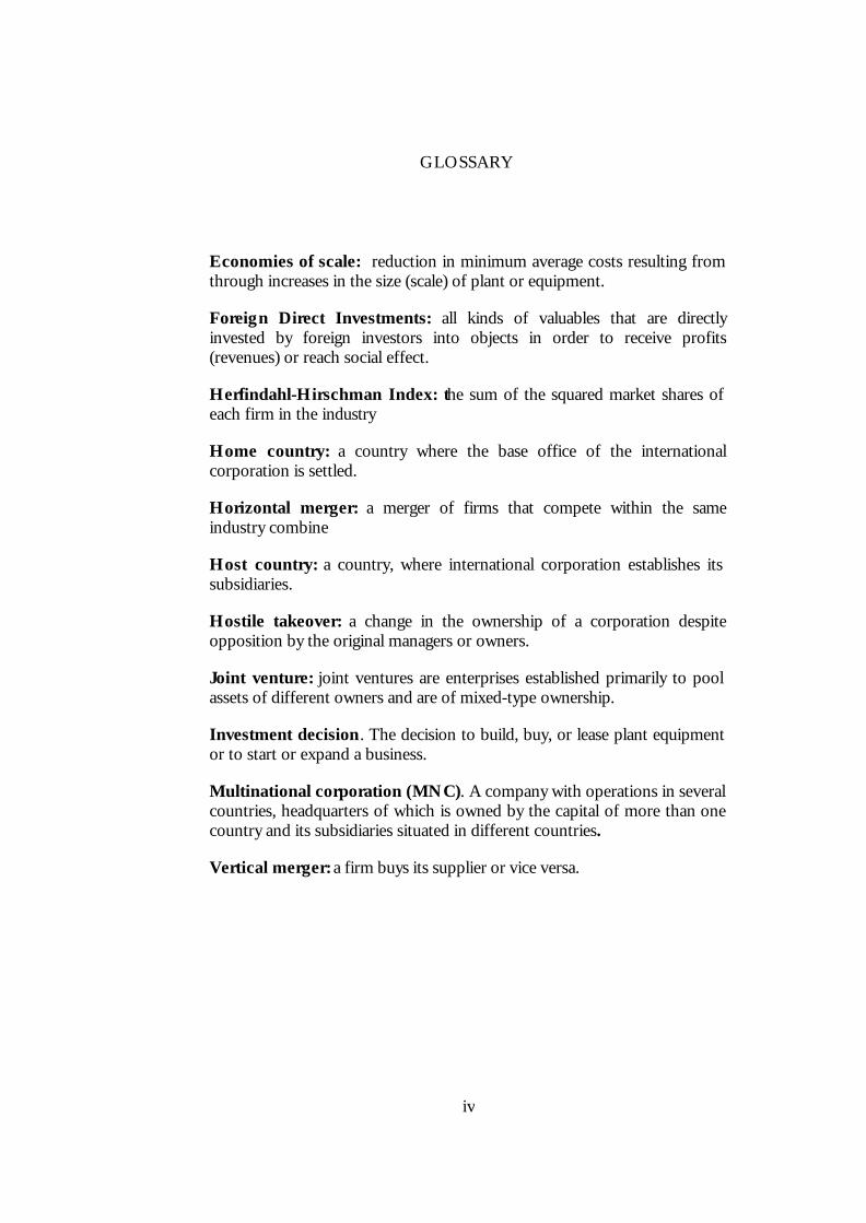
GLOSSARY

Economies of scale: reduction in minimum average costs resulting from through increases in the size (scale) of plant or equipment.

Foreign Direct Investments: all kinds of valuables that are directly invested by foreign investors into objects in order to receive profits (revenues) or reach social effect.

Herfindahl-Hirschman Index: the sum of the squared market shares of each firm in the industry

Home country: a country where the base office of the international corporation is settled.

Horizontal merger: a merger of firms that compete within the same industry combine

Host country: a country, where international corporation establishes its subsidiaries.

Hostile takeover: a change in the ownership of a corporation despite opposition by the original managers or owners.

Joint venture: joint ventures are enterprises established primarily to pool assets of different owners and are of mixed-type ownership.

Investment decision. The decision to build, buy, or lease plant equipment or to start or expand a business.

Multinational corporation (MNC). A company with operations in several countries, headquarters of which is owned by the capital of more than one country and its subsidiaries situated in different countries.

Vertical merger: a firm buys its supplier or vice versa.

S e c t i o n 1

1. INTRODUCTION

Attracting of Foreign Direct Investments (FDI) is one of the most essential

issues in reformation and modernization of the Ukrainian economy. Due to a

substantial technological lag in comparison to developed countries, Ukraine

needs foreign capital that could provide new technologies, new methods of

management and also promote development of domestic investments. The

experience of developed countries shows that investment boom starts with

adaptation of new technologies, brought with foreign capital. Dyker (1999)

emphasizes the ways, through which FDI improve economic performance of

the host countries:

• Integration of host country economy into global economy; • Increase in the aggregate level of investment • Transfer of hard technology (technology of product and process) • Transfer of soft technology (management, marketing methods) • Networking and subcontracting with domestic firms

At the same time, Ukrainian level of FDI per capita is far below that of some

transition countries, in particular the Czech Republic, Hungary or Poland. For

instance, only the USA invested 10 times more in the Polish economy than in

the Ukrainian one1. Such negligible volumes of FDI could be explained by

discouraging investment climate, presently created in Ukraine, and also

suspicious attitude toward foreign investors from government and managers

of some enterprises. Some investors think countries ex ante do not want

attract FDI. “… CEE countries were also unwilling to attract too much FDI.

In transition economies, FDI has typically meant not green field investment,

but the purchase of existing assets, usually during privatization of state-owned

enterprises. Selling state assets to foreigners is often seen as selling the family

1 From the presentation of the US ambassador Steven Pifer in NaUKMA, 2000.

2

silver and encounters widespread political resistance”, (Sinn and

Weichenrieder, 1997).

At the same time, Ukraine has a substantial economic potential, which is

utilized adequately. The main reasons for investing in Ukraine are:

• lack of competition from the domestic firms • cheap labor • potentially large consumer market

Despite these advantages, foreigners are reserved about investing in Ukraine.

Nowadays, the Ukrainian economy really needs inflows of foreign capital,

because of suspension of investment financing from government budget and

the lack of enterprises funds. Among other problems the following should be

emphasized:

• poor legislative framework • unanticipated changes in taxation • equipment deterioration • political instability

All (mentioned above) leads to Ukraine being ranked “B-“ by Moody’s

Company (Infobank, 2001), which is one of the lowest ranks in Europe.

Nevertheless, Ukraine still attracts FDI through the following activities:

• creation of joint venture firms (including sale of stock to foreigners), • creation of free economic zones

While attractiveness of FDI is an important issue for every country we should

not forget about different spillovers that FDI could cause. As a rule, FDI

gives raise to positive externalities. However, we cannot unambiguously assert

these effects of FDI in transition economies, and in Ukraine in particular. As

a rule, transition changes the way economy operates, leading to unexpected

results. Therefore FDI can bring both positive and negative externalities.

Negative spillovers could in the form of a raise in monopoly power of MNCs,

which in order to avoid competition from a Ukrainian firm, acquire and close

it.

In our paper we examine the effects on technology transfer and spillovers

deriving from FDI intensity. More specifically, we survey two problematic

3

questions, using unpublished Ukrainian micro data. Firstly, do establishments

with FDI differ in terms of performance level? Secondly, are there any

beneficial spillovers on firms that have not received FDI? We anticipate that

foreign establishments have comparatively higher levels of performance and

domestic establishments benefit from spillovers.

The data used in this research consist of 292 firm characteristics for 1998-99

and cover Odessa, Kyiv, Kharkiv and Lviv regions. The firms belong to 7

industries according to specification of EERC Research Center2.

We tackle the issue econometrically using panel data technique. The first and

second model tests whether FDI influence on labor productivity and export is

positive or not. According to the obtained results, firms with FDI have higher

labor productivity and volumes of export. In the third and forth models we

tests firms benefits from FDI vicinity. We find a positive spillover effect on

labor productivity and export volumes for non-FDI firms.

The paper is organized as follows. The next section overviews theoretical

background of the work that includes literature review, model development

and issues on the role of FDI in transition countries and Ukraine. In section 3

we describe data, econometric models and discuss the results. Conclusions

and suggestion for future research are in the last section.

2 I do thank EERC Research Center for providing the data.

4

S e c t i o n 2

2. THEORETICAL BACKGROUND

2.1. Literature review

Industrial Organization theory provides us with different approaches to

studying the direct and indirect effects of FDI on host countries. Direct

FDI effects measure the difference in firm performance between firms with

and without FDI. Indirect effects are spread through specific channels and

“examine different aspects of the interaction between MNCs and host

country residents that are plausibly related to FDI spillovers” (Blomström,

Globerman and Kokko, 1999).

2.1.1. Direct effects of FDI

Estimating direct effects, Blomström (1989) investigates differences in

labor productivity, capital-labor ratio, wage level and profitability of firms

with and without FDI. He finds that “… foreign subsidiaries in general

exhibit higher labor productivity and capital intensity than Mexican

manufacturing units of a similar size at the same four-digit industry. Foreign

firms also seem to pay higher wages.” This is explained by a higher labor

and capital quality at foreign companies. However, such indicators as the

share of labor remuneration in value added and profits per unit of capital are

lower in foreign firms. Blomström explains it by the fact that foreign

companies cover their profits to avoid some taxes. Finally, pointing to the

imperfection of his data, he concludes “Although our results indicate

differences in performance between foreign and domestic production units

in the Mexican manufacturing industry, we are unable to show that these

hypotheses are significantly different from zero”.

5

Ponomareva (2000) studies direct FDI effects in Russia focusing on whether

FDI firms perform better than domestic ones. She uses the datasets from

State Statistic Committee of Russia mostly on energy, fuel and foodstuff

production industries. A number of firms are situated in the central region,

near natural resources or metal processing centers. She develops an

econometric model where output depends on employment, capital,

economy of scale, minimum efficiency scale, existence of FDI, industry and

region. The author’s does not confirm a significant influence of foreign

majority ownership, so that firms with the prevailing share of foreign capital

do not show a better performance. Furthermore, the study finds that output

in plants with FDI is higher than that of domestic ones.

Similar research is conducted by Konings (2000) for Poland, Bulgaria and

Romania. He finds that “foreign firms perform better than firms without

foreign participation only in Poland. In Bulgaria and Romania, no robust

evidence is found of positive foreign ownership effect”. The author explains

this by the time lag needed by firms to restructure and effect on

performance productivity. According to Konings, Poland is advanced in the

transition process comparing to Bulgaria and Romania.

In another study at the macro-level Mykytiv (2000) analyzes influence of

FDI on economic growth in Ukraine is estimated. The author agrees that

FDI is commonly linked to the technological progress in the country,

because of the transfer of new technologies and inputs in innovations. This,

in turn, is the basis of argument that enterprises with foreign investments

exhibit a higher labor productivity comparing to domestically owned

manufacturing. Mykytiv also argues that FDI is positively correlated with

exports, since foreign investors often adopt export-oriented policy. It

prompts competition among local enterprises and spreads new competitive

technologies. Mykytiv (2000) develops a simultaneous model for the

economy of Ukraine and uses the Error-Correction Model to explain long-

term trends. However, he finds no significant results for the FDI influence

on economic growth. These neutral results may be the result of inadequate

country statistics.

6

2.1.2. FDI spillovers.

Technology Transfer

Describing indirect FDI effects, Blomström and Kokko (1997) discuss

transfer and technology diffusion from multinational companies to host

countries, as well as prevalent ownership of commercial technologies by

multinational companies. They consider theoretically the main technology

transfer channels such as:

• Contribution to efficiency of domestic firms • Introduction of new know-how • Transfer of techniques for inventory and quality control

Glass and Saggi (1998) develop a model in which international technology

transfer occurs through different channels. They evaluate the role that FDI

plays in technology transfer promotion. FDI is the most important channel

of international technology transfer. They argue that a faster flow of FDI to

the host country increases the rates of innovation, imitation and

international technology transfer. They also emphasize imitation as a source

of technology transfer. Finally, they suggest that rates of innovation and

imitation remain the same and FDI generate level effect only.

The technology transfer channel is also theoretically analyzed by Blomström

(1987). He concludes that “… such a transfer is a central activity of MNCs,

and this may stimulate domestic firms to hasten their access to a specific

technology”.

Ponomareva (2000) examines the impact of technological spillovers from

FDI on domestic enterprises. She mentions a positive effect from FDI

spillovers and concludes, “The effects [of FDI spillovers] depend on host

country and host industry characteristics and the policy environment in

which the multinationals operate”. The author mentions an intra-region

transfer of know-how and technology and finds that “domestic firms

located nearby multinationals benefit from this vicinity”.

7

Kinoshita (2000) examines the effect of technology diffusion from FDI in

explaining the total factor productivity growth. She uses unpublished firm-

level data of the Czech manufacturing sector for period of 1995-98. She

finds that both foreign joint ventures and foreign presence in the sector do

not have significant effects on productivity. The author finds that “the rate

of technology spillovers varies greatly among sectors. In oligopolistic sectors

such as machinery, there exists a significant rate of spillovers from having a

large foreign presence” and no spillovers in more competitive food, textile,

wood and chemical industries.

Competition

As for competition effects, Blomström (1987) describes it as an increase in

competition when multinational companies enter the host country markets.

According to Blomström, greater competition leads to a more efficient

market structure. The author argues that the Herfindahl index could be a

proxy for the estimation of this effect. However, this explanatory variable is

not significant. He explains this by the fact that “due to underdevelopment,

Mexico is a relatively small economy, but a highly protected one”. In other

words, domestic firms are legally protected from loosing their market shares

by MNCs.

Blomström and Kokko (1997) also examine the influence of international

companies on the performance of the host country, as well as the effects on

competition and industry structure in the host countries. They conclude that

FDI contributes to productivity growth and exports in host countries, yet

the exact nature of correlation between foreign and domestic firms could

vary among industries and countries: some industries are more protected by

government, some are less protected.

Ponomareva (2000) stresses the fact that competition with foreign firms

forces domestic companies to protect their market share and profits. In

contrast to the previous study, she finds negative effects. She concludes,

“increases in foreign ownership negatively affect the productivity of wholly

domestically owned firms in the same industry”.

8

Similarly, Konings (2000) finds no spillovers effects in Poland, but there are

negative spillovers in Bulgaria and Romania. He explains that “… increased

competition from FDI dominates technological spillovers to domestic firms.

It suggests that inefficient firms will loose market share due to foreign

competition, which in long run should increase the overall efficiency of an

economy”.

Furthermore, Kinoshita (1998) tries to decompose spillover effect into

competition, training, foreign linkages and demonstration effects3. The

author uses the survey data for 468 manufacturing firms in China between

1990-1992. She finds that the catch-up effect (spillovers) is “more important

for domestically owned firms than for foreign firms, which rely on the

import of intermediate goods”. The author concludes that “Chinese local

firms have survived increased competition due to the entry of more

advanced foreign firms and have accomplished rapid growth because of

this”.

Training of labor and management

Blomström (1989) mentions that the training spillover channel can be a

result of worker training by foreigners investing in human capital that

spreads not only on foreign but also on domestic firms. “In Mexico ... many

managerial people in large locally owned firms started their career in a

MNC, and management practices may in this way be substantially improved

in domestic firms”. However, he does not estimate this hypothesis

empirically.

Moreover, Kinoshita (1998) finds worker training an important source of

productivity growth. However, it has some particularities. Domestic firms

being afraid to loose their market shares, train their workers. Kinoshita

suggests, “This might have facilitated the process of intra-industry spillovers

from foreign investments”. At the same time foreign-owned firms are

unlikely to invest in the education of local workers. On the contrary, they

3 See findings on training, foreign linkages and demonstration effects below

9

“tend to maintain product quality by improving intermediate goods from

their home countries and by transferring managers from their

headquarters”.

Foreign linkage effect

Blomström and Kokko (1997) distinguish backward linkage and forward

linkage effects. A backward linkage occurs during interaction between

multinational companies’ branches with suppliers. The authors suggest that

backward linkage is associated with MNCs assistance in establishing

production facilities by suppliers, increasing quality of raw materials and

training of management. A forward linkage is associated with consumer-

MNC relationships. This channel is less evident than the previous one, and

Blomström and Kokko mention insignificance of the forward linkage effect.

Similarly, Kinoshita (1998) also included foreign linkages proxy, but finds

statistically insignificant coefficients.

Demonstration effect

Transferring of new technologies and innovations could be adopted via

simulating them. According to Blomström, Globerman and Kokko (1999),

“The successful introduction of new production techniques and new

products reduces the subjective risk surrounding the adoption of the

innovation and should, therefore promote its adoption more widely

throughout the population of potential adopters in the host country”

Blomström and Kokko (1997) suggest it as an important channel of

spillovers. They suggest, “…pure demonstration effects often take place

unconsciously … and often intimately relates to competition”.

Kinoshita (1998) determines the demonstration-imitation effect: when

domestic firms observe activity of their multinational firms they start to

imitate or copy in order to become more productive.

10

Thus, we can see that the issue of FDI and spillovers is highly appealing for

research. FDI has direct and indirect impacts. Direct FDI effects measure

difference in firm indicators between firms with and without FDI. Indirect

effects are spread through specific contacts between MNCs and domestic

firms. There are five main indirect effects found in relevant literature. The

technology transfer effect appears when domestic firms receive new

technologies and know-how for lower costs from MNCs. The catch-up

effect simply means that foreign firm catches up the share of local market or

domestic firm looses its market share. The competition effect arises when

entrance of foreign firms forces domestic firms to act more efficient in

order to save their profits and shares. The foreign linkage effect appears

when foreign owned companies use services supplied by local firms. The

training effect is a situation when foreign firms provide training for their

workers and managerial staff, which in future can be hired by domestic

firms.

11

2.2. Model development

As we can see from the previous section, there are two main subtopics of

the FDI issue:

• FDI influence on firm’s performance • Spillover estimation

Recently developed empirical models estimate two effects either

simultaneously [Ponomareva (2000), Konings (2000)] or separately

[Kinoshita (1998), Blomström (1989)].

One of the earliest econometric models for estimation of FDI influence was

developed by Magnus Blomström (1989) in his Mexican manufacturing

sector research. He estimates labor productivity as an indicator of firm’s

performance4. The model is:

)),,(,,,,( 21 FSLQLQADSCALEHKLfy ddd = , where

dy - value added in domestically owned private plants divided by total employees in these plants. dKL - the ratio of total assets to the total number of employees

dSCALE - measure of scale AD - average effective working day

1LQ - ratio of white-collar workers to blue-collar workers

2LQ - measure of labor quality H – Herfindahl index FS – share of employees in industry’s total employment in foreign plants

Among factors influencing firm performance Blomström uses capital

intensity, quality of labor force, market structure, economy of scale and

foreign presence. The last is estimated as the share of employees in an

industry employed in foreign plants. As a proxy of capital intensity

Blomström employs the ratio of total assets (book value) to the total

number of employees in the domestically owned plants. Moreover, he

suggests, “Labor productivity may also differ across plants because of scale

4 Blomström would prefer to use the ratio of net output to an index of total factor inputs, but cannot do

it because of unavailable data.

12

economies”. Diseconomies of scale are represented by the ratio of the gross

production of the largest plants in industry to gross production of an

average privately owned Mexican plant. The quality of labor force is

estimated by two variables. First, it is a ratio of white-collar to blue-collar

workers for an industry. Second, it is the error term “e” in the regression

eFSbaLQ ++= *1. The Herfindahl index, which is used as a measure

of concentration in market structure, is calculated as the sum of the squared

market share of all firms in the industry. Variable AD corrects for the

possibility of systematic differences in holidays, strikes, etc., in order to

receive a better estimation of labor productivity.

A similar approach is developed by Ponomareva (2000) in her research on

FDI spillovers in Russia. She estimates both FDI and spillover effect

simultaneously. She also uses firm’s output as a performance indicator,

which depends on capital, labor, economy of scale, FDI spillovers, FDI

presence and minimum efficiency scale. The model is:

ijijij

jijijij

espillafdiascalea

scmefacapaempaaout

++++

++++=

654

3210

*

_*)ln(*)ln(*)ln(

where, i – firm index

j – industry index out – output emp – employment cap – capital scale – economies of scale mef_sc – minimum efficiency scale fdi – dummy variable for FDI spill – spillover variable e – error term

Capital stands for fixed assets at the beginning of the year. Labor denotes

average annual employment. Like in the previous model, Ponomareva uses a

scale variable, but it is measured as an establishment’s production over the

average production in the industry. Minimum efficiency scale is estimated as

median output over average output in the industry. This variable

characterizes the distribution of firms in the industry. The FDI dummy

13

variable is valued 1 if a firm has FDI and 0 otherwise. Finally, a spillover

variable is estimated as the share of output in an industry accounted for the

foreign firms in total output.

Like Ponomareva in the previous model, Konings (2000) also estimates

both FDI and spillovers effect. He constructs a similar log-linear production

function:

ittittitititiit SpillFDIFDImalky εαηααηαααα ++++++++= 7654311

where, i – firm index, t – year index.

yit – log output kit – log of capital lit – log employment mit – log of material inputs

tη - time varying factor FDIi – share of firm hold by foreigners FDI tη – interaction of foreign ownership and time trend spill – sector level spillover variable e – error term

Compared with the previous model, Konings adds log of material inputs.

He also includes a time varying factor, which measures common aggregate

shocks in production for example technological progress or other

unobserved factors, and an interaction variable of foreign ownership and a

time trend variable, which proxies foreign ownership influence on both level

and growth of productivity. For the FDI variable Konings uses the fraction

of shares held by foreign investor, and spillover variable is represented by

the share of output accounted for by foreign firms in total output at the

two-digit NACE sector level.

There is also research that estimates spillover effects separately. Magnus

Blomström(1989) supports the idea that “[t]echnical progress can be studied

by observing changes in the best-practice technology between two periods.

The more rapid the technical progress has been, the faster the frontier has

moved”. That is why he uses relative changes in labor productivity in the

14

best practice plants within each industry between 1970 and 1975 as a

representative for technological growth. The model is:

),,,( FSMGHyfe ∆= ,

where y∆ - technical progress

H – Herfidahl index MG – market growth FS – foreign ownership share e – efficiency index

Blomström defines the market growth variable as the relative growth of

employment in each industry. He identifies a company under foreign

ownership if at least 15 percent of a company is foreign owned. Finally, the

Herfidahl index represents market structure. The dependent variable e, is

estimated in two stages. “First, the efficiency frontier is obtained by

choosing the size class within each four-digit industry showing the highest

value-added per employer”. Second, Blomström finds the ratio of industry

average5 to the value found at the first stage.

Thus, previously developed models, which estimate influence of FDI and its

spillovers on firm’s performance, can be subdivided into all-effects

estimations and separate-effects estimations. In most models, change in

added value or in output depend on FDI or spillover variable and on

additional control variables such as capital, labor, economy of scale, quality

of labor force, minimum efficiency scale, etc. Having considered mentioned

above, we develop our own models, which are described in section 3.

5 Estimated as ratio of total value added in each industry to the total number of employees.

15

2.3. FDI in transition countries

Transition countries are characterized by a need for foreign investment,

especially FDI. Below we describe the main features of investment climates

in Poland, Czech Republic, Hungary and Russia.

The Czech Republic differs from some Eastern European countries by

macroeconomic stability, well qualified labor and anticipated political

environment. According to CzechInvest6, the Czech agency for attraction

FDI, all sectors of economy are opened to a foreign presence. The Czech

government developed a standard package of incentives for manufacturing

investments in 1998. Incentives are offered for investors who invest $10

million in manufacturing through the creation of a new firm. The package

consists of duty free import of equipment, delays in value added tax

payment, training grants and additional incentives after reinvesting.

Moreover, the Czech government has created a sophisticated legal

environment based on commercial code, banking law and tax code.

According to CzechInvest data, the Czech Republic attracted the total of

US$19.3 billion of FDI in 1991-1999. Germany was the largest foreign

investor and contributed US$5.0 billion (26.2 %). The second largest

investor was Netherlands with US$4.6 billion (24.0 %). Austria and the USA

follow with US$2.3 billion (11.8%) and US$1.7 billion (9.0%), respectively.

The introduction of investment incentives resulted in a significant increase

of FDI in 1998. As for industrial allocation, the most attractive are financial

services (US$3.0 billion or 15.8%), wholesale trade (US$2.7 billion or

13.8%), non-metallic mineral products (US$1.5 billion or 8.0%) and post

and telecommunications (US$1.2 billion or 6.4 percent).

In Poland foreign investments also play a considerable role. According to

the U.S. Department of State7, all political parties and social groups support

any actions for FDI attractions in all spheres of the Polish economy except

6 Available at web-site http://www.czechinvest.org

7 Available at web-site http://www.state.gov

16

agricultural land. The Polish government has approved a comprehensive

legal framework that protects property rights and investments, provides

equal treatment for both domestic and foreign firms and allows repatriation

of profits abroad. Legislative environment is based on Commercial Code,

Law on Economic Activity, The Law on Companies with Foreign

Participation and others. The amount of FDI attracted in Poland has being

increasing since 1991 (PAIZ, 2000). For instance, cumulative FDI in 1998

was $27,279.6 million, and in 1999 - $35,170.8 million. The reasons are the

capacity of Polish markets, skilled work force and low labor costs. Total

FDI in Poland reached USD 38.9 billion in 2000. German and US

companies invested US$ 6,007.3 million (17.3 %) and US$ 5,152.9 million

(14.7%), respectively. Other large investors are France (11.1%), the

Netherlands (9.2%) and Italy (9.1%). The most attractive industries for

investing are financial services (22.4%), food processing (13.1%),

transportation equipment (12.5%), trade and repairs (9.7%), non-metal

goods (5.9%), construction (5.5%) and transport, storage and

communications (5.4%)

According to the U.S. Department of State, Hungary attracted over US$ 23

billion of FDI from 1989 to 2000, which is a significant share of all FDI

invested in Central and Eastern Europe during this period. The current

economic and legal environment encourages FDI in all areas of the private

economy. There are four main types of FDI in Hungary: establishment of a

new business, joint venture; privatization and portfolio investment, or

participation in capital raising. The major investing countries are USA,

Germany, France, Austria, and the Netherlands, followed by Italy, Sweden,

Great Britain, Switzerland, Japan, and Canada. In 1999, 55 percent of all

FDI was invested in manufacturing, followed by telecommunications (15%),

energy (13%), banking/finance (6%), and commerce (6%).

According to the U.S. Department of State, “the Russian economy has

shown strength recovering from the August 1998 financial crisis, and real

growth in the economy has helped spur limited new investment from both

domestic and foreign investors. Many problems persist, however, including

17

chronic difficulties in the overall investment climate and a weak commercial

banking sector. President Putin’s government has shown a strong interest in

attracting foreign investment and has promised to enact structural changes

that would improve the environment for investors. However, most of these

key steps have yet to be enacted.”

Among the different problems existing in Russia, crime is one of the most

viable concerns of foreign and domestic businesses, particularly those

dealing with large amounts of cash and goods. “Much crime is tied to

commercial activity, and many Russian entrepreneurs report that they must

pay kickbacks and protection to stay in business. Furthermore, foreign

investors have identified corruption as a pervasive problem, both in the

number of instances and in the size of bribes sought.” (U.S. Department of

State).

Cumulative FDI from 1992 to 1999 totals about $US 16 billion. Among the

largest investors are the following countries8: Germany - $US 6,946 million

(23.7%), USA - $US 6,349 million (21.7%), UK - $US 3,628 million (12.4%),

Cyprus - 3,440 million (11.8%) and France - $US 3,249 (11.1%).

The most attractive for FDI Russian industries in 1999 were: the fuel

industry $US 1,700 million (17.8%), trade and catering $US 1,622 million

(17.0%), consulting services $US 1,481 million (15.5), food industry $US

1,415 million (14.8), transport and communication $US 521 million (5.5%).

Eastern and Central European countries could roughly be subdivided

according their FDI attractiveness as more attractive (Poland, Czech

Republic and Hungary) and less attractive (Russia, Ukraine). Thus,

geographic factor also plays a great role in investor’s decision.

8 In cumulative terms

18

2.4. FDI in Ukraine

The collapse of the Soviet Union in 1991 created 15 independent states.

One of those countries is Ukraine, which had a land area of 604,000 square

kilometers (232,000 square miles) and a population of about 50 million. “In

the 1980s, Ukraine produced 16-18 percent of Soviet industrial output and

23-24 percent of Soviet agricultural output: in 1989 it produced 34 percent

of Soviet steel, 23.5 percent of coal, 46 percent of iron ore, 56 percent of

sugar and 36 percent of TV”, (Yegorov, 1999).

It was supposed that Ukraine be highly attractive for FDI. Ukraine had

cheap but at the same time skilled labor and available row materials.

However, investors were not in a hurry. FDI per capita in 1995 in Ukraine

was only US$13, while in Hungary it was US$1017 and in the Czech

Republic US$575.

Despite business recession, equipment deterioration, instability of

macroeconomic situation and other causes foreign investors slowly but

gradually invest in Ukraine, except in areas prohibited by law. Government,

financial intermediaries and firms with FDI actively operate in the

investment market. The government provides formal rules or legislation

environment at both national and local levels, though officials are often

interested in political power and private benefit. As for informal rules,

“...corruption follows directly from the degree of discretion officials have in

granting approvals for private business. Unofficial payments have to be

made at all stages of the licensing and permissions process” (Kudina, 1998).

Another actors in the market are financial intermediaries or security brokers,

who act as agents for investors. They compete at the investment market

supplying consulting services. KINTO Investments and Securities, Alpha

Capital, Dragon Capital are leaders at the market. “The leading Ukrainian

securities company, KINTO Investments and Securities, was formed with a

substantial contribution from Wasserstein Parella of the US and European

Privatization and Investment Corp. In turn, KINTO has created a number

19

of daughter companies, which operate on the Ukrainian equity market”

(Yegorov, 1999).

Foreigners mostly invest through creation of own firms (for example,

Cargill’s new seed processing plant in the Donetsk Region) or buying equity

(For example Irish CRH, which bought controlling interest of cement plant

in the Khmelnitsky Region). Foreign investment has the following forms:

• Foreign exchange • Domestic currency (reinvesting) • Any movable and immovable property • Equity • Corporate rights • Immaterial assets (know-how, software)

Investments in Ukraine are formally regulated by laws and other legal acts.

The following laws should be emphasized:

• The Law “On Foreign Investing Regime”, dated March 19, 1996 • The Law “On Foreign Investments” dated March 16, 1992 • The Law “On State Program of Encouraging Foreign Investments

in Ukraine”, dated December 17, 1993 • Cabinet Resolution on a Foreign Investment Regime, dated May

20, 1993;

The main features of Law “On Foreign Investing Regime” are:

• Registration requirement of foreign investments with local authorities

• Regulation of types of foreign investments • Privileges for foreign investors • Guarantees for profit repatriation • Exemption of custom duties for foreign contributions to statutory

fund.

In order to attract more investors, there are provisions on legislature

changes in Law “On Foreign Investments”:

• Foreign investors are guaranteed protection against changes in legislature for 10 years

• Guarantees against illegal nationalization • Compensation and reimbursement of foreign investors losses

(nationalization)

20

• Guarantees if investment activity is terminated (repatriation of profits and invested assets).

• Guarantees for profit repatriation • State registration and control for foreign investments

The law “On State Program of Encouraging Foreign Investments in

Ukraine” describes ways to attract more FDI into agriculture, light, fuel,

medicine, chemical and transport industries.

However, these laws cannot fully clarify ambiguity in the FDI legal

environment. The government can issue and an unanticipated amendment

in the middle of year, when plans for most companies’ development are

already established. Moreover, numerous cases of corruption and bribery are

apparently not conductive to the attraction of FDI.

According to the official statistical office, Derzhkomstat, FDI in Ukraine

has reached the total of $3.25 billion since 1992. The United States has

invested $589 million and has become the largest investor; the Netherlands

follows with $301 million. Other big investors are Russia ($288 million),

Great Britain ($243 million), and Germany ($229 million)

The most important for FDI industries are machinery (13% of total FDI),

and food industry (21%). Domestic trade also plays a significant role in FDI

attraction (16%) (Derzhkomstat, 2000).

According to the Institute of Reforms (2000) there are many differences in

FDI attractiveness by regions9. Kyiv City is the most attractive region in

Ukraine. It has a comparatively developed transport and communication

systems, infrastructure, financial institutions. The average salary in Kyiv is

twice than the average in Ukraine. As on June 2000, $1.2 billion were

invested in the city, 32,9% from the USA, 16.5% from Cyprus, 9.8% from

Austria, 6.8% - Hungary and 4.2% from Switzerland.

9 The ranking of investment attractiveness is based not only on investment but also on economic,

infrastructure, social regional features.

21

The second in the ranking of investment attractiveness (Institute of

Reforms, 2000) is the Donetsk region. As of July 2000, due to the creation

of free trade zones “Donetsk” and “Azov” and attractive economic

situation investors, contributed to the Donetsk region $293.5 million.

Dnipropetrovsk, Lviv, Zaporizhia and Kharkiv could also be named as

leaders. These regions attracted $184.33 million, $125.85 million, $218.00

million and $88.86 millions, respectively. Next group is the “followers”. It

consists of the Odessa ($190.12 million), Kyiv excluding the city ($302.9

million), Poltava ($211.12 million) regions, and the Crimea Republic ($150.1

million). Each of these regions attracted a significant amount of FDI but

because of various reasons10 lags behind the leading regions. Chernivtsi

($8.16 million), Zakarpattja ($81.73 million), Mykolaiv ($44.87 million),

Lugansk ($30.25 million), Ivano-Frankivsk ($37.64 million), and Kherson

($32.19 million) regions are included in the “main” group. The regions of

this group have variega ted indicators. For example the Ivano-Frankivsk

region has ranked 13th in the stocks parameter, but there is no regional

company listed in PFTS, the Ukrainian index. The group of “outsiders” is

characterized by an undeveloped business infrastructure and consists of

Chernigiv ($46.78 million), Vinnytsja ($17.06 million), Rivne ($44.79

million), Ternopil ($19.65 million), Khmelnitsky ($14.67 million), Sumska

($34.56 million), Kirovograd ($17.96 million), and Cherkasy ($103.60

million).

Thus, on the one hand Ukraine could potentially be attractive to foreign

investors. It is possible to earn huge profits. On the other hand, it is

extremely risky to put money into Ukrainian firms due to political instability

and vulnerable legislature.

10 For example the Odessa region does not have a developed financial infrastructure, its level of

production significantly depends on companies such as Odessa refinery or Ukrtatnafta in the Poltava region.

22

S e c t i o n 3

3. EMPIRICAL PART

As we can see from the previous part, FDI and spillover issue has

substantial theoretical background. Unfortunately, nobody has ever

researched the topic in Ukraine. Having stated the main question of paper

“Does Ukraine benefit from FDI?” we test for direct and indirect FDI

effects on labor productivity and export volumes. In our research we use

unpublished firm level data from the EERC Research Center.

3.1. Data description

The data used in this research consist of two EERC Research Center

datasets. The first includes micro-level information on fixed assets, labor

force, sales, export, import, barter operations, and industry-region

information. The second contains information on FDI presence in certain

firms.

To present such variables as capital we could use different estimations of

fixed assets. According to a theoretical study (Ponomareva, 2000), the

balance sheet value could be the best proxy for capital, since it reflects real

capital capacities of the firm. All data are constant 1998 prices, cobverted

using producer price index from the UEPLAC(2000) web site11 (See Table

1).

There are 292 observations for manufacturing firms for 1998 and 1999.

25% of them have some FDI. A firm is assumed to have FDI when12:

11 Available at http://www.ueplac.kiev.ua

12 Firms unwillingly report on FDI availability. Therefore, the EERC Research Center used questionaires about changes in FDI in order to find the FDI existence in companies

23

• They had changes in FDI during last period • They had foreign ownership13

The dataset covers Lviv, Kyiv, Odesa and Kharkiv regions, which represent

West, Center, South and East of Ukraine, respectively. Regional distribution

with frequencies and percentages is described in Table 2. As can be seen

from the Table 2, the share of Kyiv, Lviv and Kharkiv regions is 30% each,

while the share of Odesa region is 10%. This may be explained by the fact

that Ukrainian South is less industrialized than central or eastern areas, and

the fact of unwillingness of Odesa region’s managers to take part in EERC

survey.

Table 1. Statistic characteristics of variables used in research.

All firms FDI firms Variable

Mean Std. Dev. Mean Std. Dev.

Balance value of fixed

assets, UAH 1998

17324.32 54366.9 5904.55 12853.74

Sales, UAH 1998 5026.05 15245.07 3353.26 7379.38

Import, UAH 1998 902.15 3525.32 1548.95 3914.26

Production, UAH 1998 5169.32 15474.25 3948.94 10837.29

Labor, workers 457 1019 255 508

Export, UAH 1998 852.12 3801.31 1136.95 4246.77

13 We assumed that firms with foreign ownership should have FDI in either material or at least non-

material form.

24

The dataset covers 7 industries. Most of the firms are involved in food

industry (25%) or in metal processing (20%). A large number of firms do

not identify themselves with any particular industry (22%). The industry

distribution of firms is summarized in Table 3.

Table 2. Region distribution of firms.

All firms FDI firms Region

Frequency Percentage Frequency Percentage

Kyiv region 88 30.14 22 30.14

Lviv region 90 30.92 26 35.62

Kharkiv region 89 30.48 22 30.14

Odesa region 25 8.56 3 4.10

Table 3. Industry distribution of firms

All firms FDI firms Industry

Frequency Percentage Frequency Percentage

Metallurgy 24 8.22 5 6.85

Metal processing 58 19.86 8 10.96

Wood and Paper 15 5.14 5 6.85

Construction

materials

26 8.90 5 6.85

Light 30 10.27 9 12.33

25

Food 74 25.34 18 24.66

Others 65 22.26 23 31.51

The ownership structure of available data is depicted in Table 4. A

significant share of firms (36%) constitutes an unspecified form of

ownership14. Workers own 17% of firms in the sample. Other physical

entities are either retired persons or those who bought shares during

certificate auctions.

Some firms with foreign ownership were added to the original dataset in

order to increase the sample of firms with FDI15.

Table 4. Ownership distribution of firms16

Ownership Frequency Percentage

Workers 49 16.78

Managers 13 4.45

Government 7 2.40

Other physical entities 27 9.25

Other Ukrainian companies 29 9.93

Other foreign companies 61 20.89

Other 106 36.30

14 See in appendices: A4. Questionnaire. Total information about enterprise in appendices, question #3.

15 Total amount of added firms is about 45.

16 On the basis on major ownership.

26

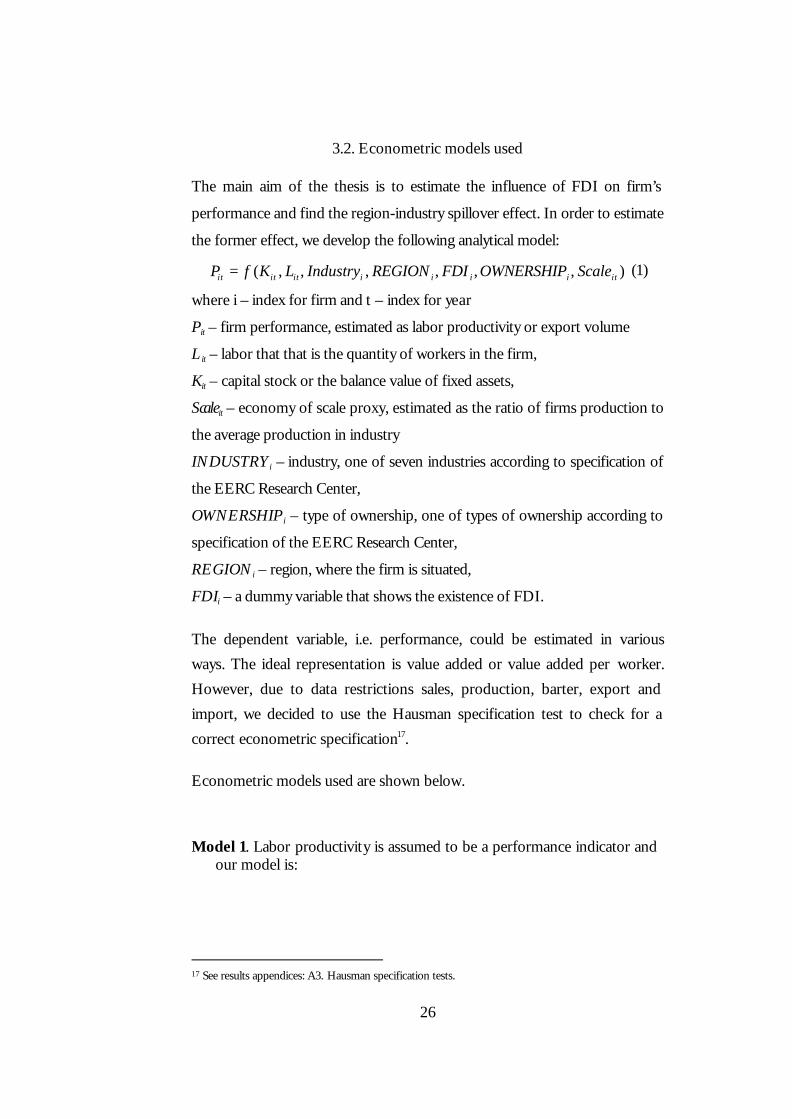
3.2. Econometric models used

The main aim of the thesis is to estimate the influence of FDI on firm’s

performance and find the region-industry spillover effect. In order to estimate

the former effect, we develop the following analytical model:

),,,,,,( itiiiiititit ScaleOWNERSHIPFDIREGIONIndustryLKfP = (1)

where i – index for firm and t – index for year

Pit – firm performance, estimated as labor productivity or export volume

Lit – labor that that is the quantity of workers in the firm,

Kit – capital stock or the balance value of fixed assets,

Scale it – economy of scale proxy, estimated as the ratio of firms production to

the average production in industry

INDUSTRYi – industry, one of seven industries according to specification of

the EERC Research Center,

OWNERSHIP i – type of ownership, one of types of ownership according to

specification of the EERC Research Center,

REGIONi – region, where the firm is situated,

FDIi – a dummy variable that shows the existence of FDI.

The dependent variable, i.e. performance, could be estimated in various

ways. The ideal representation is value added or value added per worker.

However, due to data restrictions sales, production, barter, export and

import, we decided to use the Hausman specification test to check for a

correct econometric specification17.

Econometric models used are shown below.

Model 1. Labor productivity is assumed to be a performance indicator and our model is:

17 See results appendices: A3. Hausman specification tests.

27

itii

iiit

it

it

it

OWNOINDUSTRYS

REGIONRFDILK

constLY

ε

αα

δδδ

σσσ

ρρρ

++

++++=

∑∑

∑

==

=

6

1

6

1

3

121 lnln

(2)

where

FDIi, is a dummy variable taking the value 1 if the firm has ever had foreign

direct investments, and 0 otherwise.

REGIONi, INDUSTRYi are dummies, which specify an industry and region,

respectively. For region dummies Odesa region is the base and R1 denotes

Kyiv region, R2 – Lviv region and R3 - Kharkiv region. Unspecified industry is

the base for industry dummies and other dummies are: S1 – metallurgy, S2 –

metal processing, S3 – wood and paper industry, S4 – construction materials

industry, S5 – light industry and S6 – food industry.

OWNoi – are dummies that determine type of ownership. Unspecified kind

of ownership is the base for ownership dummies. We denote O1 – workers

ownership majority, O2 – management, O3 – state, O4 – other physical

entities, O5 – other Ukrainian companies and O6 – other foreign companies.

Our Hypotheses for the model 1 are the following:

H0: á2=0: FDI does not affect labor productivity

H1: á2>0: FDI has a positive influence on labor productivity

We anticipate the rejection of our H0.

Model 2. Performance is measured by export volume. Theoretically, if a firm

exports more, it has comparative advantage, which is a positive fact. The

second model is the same as model 1, but we add economy of scale proxy,

estimated as the ratio of firm’s production to the average production in

industry: We also use capital and labor variable separately instead of labor

productivity.

28

itiiti

iiititit

OWNOScaleINDUSTRYS

REGIONRFDILKconstExp

ε

ααα

δδδ

σσσ

ρρρ

+++

+++++=

∑∑

∑

==

=

6

1

6

1

3

1321 lnlnln

(3)

Hypotheses for model 2:

H0: á3=0: FDI does not affect export volumes,

H1: á3>0: FDI has a positive influence on export

We anticipate the rejection of H0.

Endogeneity is a problem associated with models 1-2. It is typical in Ukraine

that firms with FDI have higher labor productivity and firms with larger

labor productivity attract more FDI. In other words, foreigners make

Ukrainian firms to operate more efficient and the best firms also attract

FDI. The same links can be traced between FDI and export. Firms with

FDI have larger volumes of export and conversely large volumes of export

magnetize FDI.

In order to solve this problem we used the 2 stage methodology. While FDI

is highly correlated with export, the latter, in turn, is not closely correlated18

with labor productivity. Therefore, we construct the following measure:

ititi EXPconstFDIprobit εα ++= ln)( (4)

and then, using the GLS in order to avoid heteroscedasticity problem:

itii

iiit

it

it

it

OWNOINDUSTRYS

REGIONRFDILK

constLY

ε

αα

δδδ

σσσ

ρρρ

++

++++=

∑∑

∑

==

=

6

1

6

1

3

121 lnln

(5)

18 R2 =0.15

29

Thus, we estimated the real effect of FDI on labor productivity. Similarly,

export is estimated as an indicator of firm performance:

itit

iti L

YconstFDIprobit εα ++= ln)( (6)

itiiti

iiititit

OWNOScaleINDUSTRYS

REGIONRFDILKconstExp

ε

ααα

δδδ

σσσ

ρρρ

+++

+++++=

∑∑

∑

==

=

6

1

6

1

3

1321 lnlnln

(7)

We anticipate that FDI has a positive effect on firm’s performance

estimated as labor productivity or export.

In models 3-4 we investigate whether a firm that does not receive FDI

benefits from FDI in other firms in its industry-region. In other words, we

want to estimate the influence of FDI intensity, which is represented as a

share of investment in a certain region-industry, on performance of firms

that do not have FDI.

There is a less potential for “endogeneity”19, as we do not expect the

productivity of firms that do not receive any FDI to be affected by the

proportion of FDI in other firms in their industry-region. It is not likely that

FDI in the industry-region should somehow be correlated with the labor

productivity of firms that do not get any FDI. To control for unobserved

heteroscedasticity we use the GLS in models 3-4.

Model 3. We use the labor productivity as a measure of firm performance,

and the model is:

itiiiit

it

it

it INDUSTRYSOWNOSPILLK

constLY

ελασ

σσδ

δδσδ +++++= ∑∑==

6

1

6

11 lnln (8)

19 I thank Inessa Love from Columbia University for clarifying this point.

30

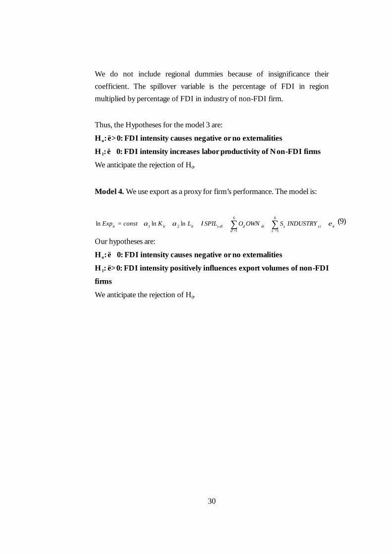
We do not include regional dummies because of insignificance their

coefficient. The spillover variable is the percentage of FDI in region

multiplied by percentage of FDI in industry of non-FDI firm.

Thus, the Hypotheses for the model 3 are:

Ho: ë>0: FDI intensity causes negative or no externalities

H1: ë�0: FDI intensity increases labor productivity of Non-FDI firms

We anticipate the rejection of H0.

Model 4. We use export as a proxy for firm’s performance. The model is:

itiiiititit INDUSTRYSOWNOSPILLKconstExp ελαασ

σσδ

δδσδ ++++++= ∑∑==

6

1

6

121 lnlnln (9)

Our hypotheses are:

Ho: ë�0: FDI intensity causes negative or no externalities

H1: ë>0: FDI intensity positively influences export volumes of non-FDI

firms

We anticipate the rejection of H0.

31

3.3. Analysis of results

In order to test all four hypotheses we tested 4 models. Our findings for the

hypotheses testing are described in tables 5-8. Model 1 is estimated as

variations of Equation 5. We test for FDI impact on labor productivity.

Table 5. Regression results for the FDI effect on labor productivity.

it

it

LY

ln it

it

LY

ln it

it

LY

ln it

it

LY

ln

constant 3.110221 *** (.3798949)

3.36888*** (.6094581)

3.797782*** (.5813996)

3.361068 *** (.6017184)

it

it

L

Kln -.0321387

(.0954852) -.0958973 (.0990565)

-.0777378 (.0874039)

-.0483727 (.0878096)

FDI .7544024*** (.1440682)

.7314491*** (.1436722)

.8042352*** (.137226)

.7737273*** (.1398052)

Kyiv region .1963453 (.4919964)

.0382721 (.4099749)

.0755219 (.4087269)

Lviv region -.5243072 (.5092676)

-.3578108 (.4218442)

-.3236778 (.4304532)

Kharkiv region

-.00652 (.5054732)

.0584154 (.4184861)

.1697789 (.420667)

Metallurgy industry

-.0532733 (.3458821)

.1002837 (.3539814)

Metal processing

-1.2091*** (.2727451)

-1.105147*** (.2791934)

Wood and paper

.2423589 (.5650992)

.069621 (.5597583)

Construction materials

-1.748438*** (.6451326)

-1.8427 *** (.661591)

Light industry

-.9461021*** (.3357283)

-1.122641*** (.3374742)

Food industry .8116791*** (.3107219)

.8844425 *** (.3141468)

Workers ownership

(.5302774) .3298891

Managers .6611196 (.4943387)

State .0459265 (.4322602)

Physical entities

.4110196 (.3146988)

Ukrainian companies

-.371814 (.3498654)

Foreign companies

.5729147 ** (.2739975)

R2 0.0671 0.1121 0.4654 0.5010 In parentheses are standard errors; *, **, *** mean 10%, 5% and 1% significance level respectively.

32

It could be concluded from Table 5 that FDI influence is positive and

significant for all model variations. Moreover, regional dummies are not

significant that suggests no significant difference among Kyiv, Kharkiv,

Odesa and Lviv regions. As for the industry dummies, labor productivity is

lower in metal processing (S2), construction materials (S4) and light industry

(S5) and higher in food industry (S6). Among ownership dummies, only the

foreign ownership dummy is significant and has a positive impact. Foreign

owned firms have higher labor productivity. So, we could suggest that our

zero hypothesis is rejected statistically.

In order to test our second hypothesis we estimated the model from

Equation 7. The results are in Table 6. The FDI dummy is significant and

positive, which suggests that H0 is econometrically incorrect. Expansion in

the export volume depends on labor. Regional variables are not significant,

which could signify the absence of regional differences. Light industry (S5)

firms have higher export volume. This could indicate that light industry is

more export-oriented than others, because it is labor intensive and Ukraine

has cheap and hill-skilled labor. The coefficients of other industry dummies

are not significant.

Further, we look for the ownership effect. Only two dummies, for the state

(O3) and foreign ownership (O6), are significant. Export orientation of

foreign owners can be explained by the fact that production in Ukraine is

less expensive than in some other countries due to cheap, high-skilled labor

and tax privileges. The significance of state ownership could be a result of

government subsidies. Moreover, state-owned companies could have direct

and indirect advantages. Direct advantages could be explained through tax

holidays, while indirect advantages could imply cheaper prices for gas,

electricity and utilities, which are subsidized by government.

33

Table 6. Regression results for the FDI effect on export.

itExpln itExpln itExpln itExpln

constant 746.0346*** (123.3835)

739.6532*** (128.3026)

952.2325*** (166.672)

844.6346*** (163.6355)

itKln -.065302 (.1685712)

-.0754216 (.177256)

.0375476 (.17749)

.0927884 (.1679689)

itLln 1.053925*** (.2556936)

1.059116*** (.2603795)

.8663591*** (.2800036)

.9558322*** (.2707489)

FDI 46.0487*** (7.622021)

45.65519*** (7.92957)

58.7844*** (10.30754)

52.22984*** (10.11333)

Kyiv region .1402472 (.7403931)

.0381235 (.734901)

-.1492532 (.6920088)

Lviv region .00934 (.7729364)

-.0672211 (.758352)

-.4810016 (.7283313)

Kharkiv region .0473668 (.7619232)

-.1459191 (.7497495)

-.4511203 (.7099927)

Metallurgy industry

.2150633 (.6217436)

.3292866 (.6009516)

Metal processing

.7478811 (.5235675)

.789942 (.4958547)

Wood and paper

.4667229 (1.011058)

.315329 (.9461807)

Construction materials

.1945991 (1.184627)

.725286 (1.143566)

Light industry 1.660828 *** (.6113901)

1.410261** (.5931065)

Food industry -.9703221 * (.5672528)

-.8042281 (.543708)

Scale -.0026378 (.0595256)

-.0159139 (.0576004)

Workers ownership

.0152263 (.5693204)

Managers .0744125 (.8567416)

State 1.135162 (.7350317)

Physical entities

.5281672 (.5320371)

Ukrainian companies

.9791046 ( .5998799)

Foreign companies

2.082235*** (.4919346)

R2 0.3202 0.3215 0.4126 0.5036

In parentheses are standard errors; *, **, *** mean 10%, 5% and 1% significance level respectively.

Finally, we test for spillovers influence on non-FDI firm’s performance.

Model 3 is described by equation 8. We estimate FDI intensity (spillover)

effect on non-FDI firms performance, measured as labor productivity.

According to the results in Table 7, the spillover variable (FDI intensity) is

positive and significant at the 1% level. We could suggest that positive FDI

spillovers exist, but their effect is comparatively low because of small

volume of FDI in Ukraine. Furthermore, firms owned by other Ukrainian

companies (O5) operate worse than firms with other ownership types. This

34

could be explained by competition. Business rivals buy shares each other to

have better access to raw materials Non-FDI firms have lower labor

productivity in metal processing (S2) and wood industries (S3). At the same

time, the metallurgy industry (S1) creates positive externalities.

Table 7. Regression results for the spillovers effect on labor productivity.

it

it

LY

ln it

it

LY

ln it

it

LY

ln it

it

LY

ln

constant .8387315 *** (.2503692)

.9339324 *** (.2723761)

.8037184 *** (.2917585)

.7770575 *** (.2837662)

it

it

L

Kln

.1707783 ** (.0788923)

.17281 ** (.0795979)

.2292445 *** (.0755159)

.2267631 *** (.0753785)

spillover .0029564 *** (.0007592)

.0029796 *** (.0007643)

.0022251 *** (.0007798)

.0023776*** (0007746)

Workers ownership

-.2742787 (.2454183)

-.155701 (.2276825)

Managers .0620174 (.4177473)

.1221477 (.3963747)

State -.2565311 (.5136659)

.4522285 (.4829886)

Physical entities .0554883 (.2879311)

.0297117 (.2631004)

Ukrainian companies

-.5306005* (.3026857)

-.5987747** (.2797578)

Foreign companies

.7990214 (.9661738)

.0781827 (.8985468)

Metallurgy industry

.5885331 * (.3363792)

.5185387 (.334257)

Metal processing

-.7742763*** (.2774144)

-.8045659*** (.2710271)

Wood and paper

-.8716325** (.4409653)

-.8462005** (.4235343)

Construction materials

-.0539755 (.3273139)

-.1288253 (.3251478)

Light industry -.4108193 (.3406818)

-.4664606 (.3348827)

Food industry .7299265 (.2758278)

.6428868 (.2670187)

R2 0.0898 0.1091 0.2734 0.2504

In parentheses are standard errors; *, **, *** mean 10%, 5% and 1% significance level respectively.

Finally, our model 4 where performance is estimated as export volumes is in

the Equation 9.

The results of the model are depicted in Table 8. The spillover variable is

statistically significant which implies the rejection of Ho for the model 4.

The coefficient by spillover variable is low and smaller less than the

coefficient of the labor variable, which is also significant. While industry

35

dummies are not significant, firms owned by state (O3) and other physical

entities (O4) do benefit from the type of ownership.

Table 8. Regression results for spillovers influence on volumes of export.

itExpln itExpln itExpln itExpln

constant -1.986797*

(1.081524) -2.522509 ** (1.050605)

-2.167826** (1.012107)

-2.589027 (1.160966)

itLln 1.174555*** (.1607732)

1.169415*** (.1585468)

1.164557 *** (.1541413)

1.22317 *** (.1694424)

spillover .0029216 * (.0016981)

.0028104** (.00142)

.0028077 * (.0014433)

.0032366* (.0017117)

Workers ownership

.3753603 (.610116)

Managers .7417539 (.9254058)

State 1.190222 (.7258599)

1.324532* (.7662441)

Physical entities

1.051411* (.5439513)

1.233253** (.5864281)

Ukrainian companies

.8572546 (.6658557)

1.129888 (.7260139)

Metallurgy industry

.7174181 (.7039667)

.9029099 (.5839055)

.9589779 (.5877421)

.4705539 (.7169181)

Metal processing

-.3159037 (.5702525)

-.6071945 (.5736704)

Wood and paper

.9759838 (2.033107)

1.248586 (2.006702)

Construction materials

-1.185085 (1.168831)

-1.144203 (1.191918)

Light industry .7235154 (.7583744)

1.064151* (.6428224)

.9691074 (.6497758)

.5397828 (.7755485)

Food industry -.283287 (.7596769)

-.550465 (.7884481)

R2 0.3659 0.3932 0.3535 0.4082

In parentheses are standard errors; *, **, *** mean 10%, 5% and 1% significance level respectively.

36

S e c t i o n 4

4. CONCLUSIONS AND SUGGESTION FOR FUTURE RESEARCH

The issue of FDI and spillovers is highly appealing for research, because

FDI could have not only positive, but also negative externalities. FDI also

has direct and indirect impacts. Direct FDI effects measure differences in

firm indicators between firms with and without FDI. Indirect effects are

spread through interactions between foreign and domestic firms. There are

five main indirect effects found in relevant literature: technology transfer,

catch-up, competition effect, foreign linkage effect and training effect.

Using unpublished micro-level annual data for 292 firms during 1998-99, we

test for statistical significance of FDI impact on labor productivity (Model

1) and export volume (Model 2). Furthermore, we investigate spillover

effect in Models 3-4.

The results reported in the paper imply that the presence of FDI has a

positive influence on both labor productivity and exports. Regional variables

are not significant that could imply the absence of differences for Kyiv,

Kharkiv, Odesa and Lviv regions. There is also a small spillover effect that

signifies positive impact of FDI environment on such non-FDI firms’ labor

productivity and export volumes. Hence, small volumes of FDI cannot have

much influence on performance.

As for industry dummies in Model 1, firms from metal processing,

construction materials and light industry have lower, while enterprises in

food industry have higher labor productivity. We can suggest from model 2

that light industry companies export more then firms from other industries.

According to Model 3, metal processing and wood industries have lower

labor productivity for non-FDI firms than others industries. At the same

time, metallurgy industry creates positive externalities.

37

Among ownership dummies in Model 1 and 2, foreign ownership dummies

are significant and have a positive impact. Export orientation of foreign

owners can be explained by a greater efficiency of foreign owners. The

significance of state ownership in Model 2 could be a result of government

subsidies, tax privileges or other policies. According to Model 3 results,

firms owned by other Ukrainian companies operate worse than firms with

other types of ownership.

Despite popularity in other transition countries, the topic of the effect of

FDI on firm performance is rarely described in Ukrainian applications. As

for the future research, ideally, it would be challenging to assess the effects

of FDI volumes on firm performance. Moreover, the sample of 292 firms

may not accurately describe the real situation and it is important to expand

the sample. Also, it would be advantageous to estimate the effects of

industry and regional spillovers separately. Finally, output per worker and

export could not be the best indicators of firm’s performance. We expect

value added and value added per worker to be the better measures.

WORKS CITED

Blomstrom Magnus. 1999. “Internationalization and Growth: Evidence from Sweden”, Stockholm School of Economic Working Paper No. 375.

----. 1989 “Foreign investment and Spillovers”, Routledge.

----, Ari Kokko. 1997. “How Foreign Investment Affects Host Countries?”, The World Bank Policy Research Working Paper, No.1745.

-----, -----, and Steven Globerman. 1999. “The Determinants of Host Country Spillovers from Foreign Direct Investment: Review and Synthesis of the Literature”. Stockholm School of Economic Working Paper No. 339.

Davies, Howard. 1977. “Technology Transfer Through Commercial Transactions”, Journal of Industrial Economics, Vol. 26, No. 2, pp.161-175.

Djankov, Simeon, Hoekman Bernard. 1998. “Avenues of Technology Transfer: Foreign Investment and Productivity Change in Czech Republic”, Center for Economic Policy Research, Discussion Paper, No.1883.

Dyker, David A.. 1999. Foreign Direct Investment and Technology Transfer in the Former Soviet Union”, Cheltenham, U.K. and Northampton, Mass.: Elgar; Distributed by American International Distribution Corporation, Williston, Vt.

Estrin S. Rosevear A. 1999. “Enterprise performance and ownership: The case of Ukraine”, European Economic Review, 43 pp.1125-1136.

Findlay, Ronald. 1978.“Some Aspects of Technology Transfer and Direct Foreign Investment”, The American Economic Review, vol.68, No.2, pp.275-279.

Glass Amy Jocelyn and Kamal Saggi. (1998) Intellectual property rights and Foreign Direct Investments. Mimeo. Ohio State University.

Green, William H. 2000. Econometric Analysis. Prentice Hall.

Grossman, G., and Helpman, E. 1991a. Innovation and Growth in the Global Economy. MIT Press.

Gujarati, Damodar N. 1995. Basic Econometrics, Mc Graw Hill, Inc.

Johnson, Jack and John DiNardo. 1997 Econometric Methods. McGraw-Hill.

Herasymenko, V. 2000. “Foreign Direct Investment and its Role for Transition Countries”, materials of international conference “Crossboarder Capital Flows in Transition Economies”, mimeo., EERC-Kyiv.

Institute of reform (2000). Å ê î í î ì ³ ÷ í ³ åñå: ðåéòèíã ³íâåñòèö³éíî¿ ïðèâàáëèâîñò³ ðåã³îí³â Óêðà¿íè ó 1- ìó ï³âð³÷÷³ 2000 ðîêó. Vol 4.

Jensen, Richard, Marie Thursby.1987. “A Decision

2

Theoretic Model of Innovation, Technology Transfer, and Trade”, Review of Economic Studies, vol.54, No.4, pp.631-647.

Kinoshita, Yuko. 1998. Technology Transfer through Foreign Direct Investments, mimeo., CERGE

_____. 2000. R&D and Technology Spillovers via FDI: Innovation and Absorptive Capacity, mimeo., CERGE

Konings, Josef. 2000. The Effects of Foreign Direct Investments, on Domestic Firms: Evidence from Firm Level Panel Data in Emerging Economies. Center for Economic Policy Research, Discussion Paper, No.2586.

Kudina, Alina. 1999. “The Motives for Foreign Direct Investment in Ukraine, Master’s Thesis, mimeo., EERC-Kyiv.

Loo, Frances Van.1977. “The Effect of Direct Foreign Investment on Investment in Canada”, Review of Economics and Statistics, vol.59, No.4, pp.474-481.

Markusen, James, Rutherford F. Thomas, David Tarr. 2000. “Foreign Direct Investment in Services and Market for Expertise?”, NBER Working Paper, No.W7700

Mykytiv, A. 2000. “Does Foreign Direct Investment Have Positive Impact on Economic Growth in Transition Economies? A Cross-Country Study”, materials of international conference “Crossborder Capital

Flows in Transition Economies”, mimeo., EERC-Kyiv.

Oleksiv, M. 2000. “What Factors Affect Foreign Direct Investment Flow in Ukraine”, materials of international conference “Crossborder Capital Flows in Transition Economies”, mimeo., EERC-Kyiv.

Ponomareva, N. 2000. “Foreign Direct Investment in Russia: Effects on Productivity”, materials of international conference“ Crossborder Capital Flows in Transition Economies”, mimeo., EERC-Kyiv.

Ramachandran, Vijaya.1993. “Technology Transfer, Firm Ownership, and Investment in Human Capital”, Review of Economics and Statistics, vol.75, No.4, pp.664-670.

Sinn, Hans Werner and Weichenrieder Alfons 1997. Foreign Direct Investment, Political Resentment and the Privatization Process in Eastern Europe, Economic Policy: A European Forum; 0(24), April 1997, pp177-98.

Yegorov Igor, 1999. Foreign direct investments in Ukraine: First results, Tendencies and Prospects”, Foreign Direct Investments and Technology Transfer in the Former Soviet Union. pp.155-188

The Law of Ukraine “On Foreign Investments”. 1992,

The Law “On The Foreign Investing Regime”, 1996,

The Law “On The State Program of Encouraging of Foreign Investments in Ukraine”,1993,

3

APPENDICES

A1. Graphs

Regional Distribution of Dataset

Kyiv region30%

Lviv region31%

Odesa region9%Kharkiv region

30%

Industry distribution in dataset

Metallurgy8%

Light10%

Food26%

Others22%

Construction materials

9%

Wood and Paper5%

Metal processing20%

4

A2. Stata 6.0 do-file program

use "e:\stata\panel.dta", clear log using e:\stata\results.log, replace iis eerc tis year /*Variables*/ gen lnk=log(bfa) /*Capital:*/ gen lnl=log(lab) /*Labor*/ gen spil=rinv*ispil/* FDI intensity : %industry*%region*/ gen lny_l=log(y/lab) /*Production per worker*/ gen lns_l=log(a/lab) /*Sales per worker*/ gen lnk_l=log(bfa/lab) /*Capital per worker*/ gen lbar=bar/a /*% of Barter*/ gen lexp=log(exp) /* Export*/ gen lexp_l=log(exp/lab) /* Export per worker*/ gen exp_s=exp/a /* % of export in sales*/ egen scale1 = mean(y), by (i1-i6) gen scale = y/scale1 /*Economy of Scale:*/ /*Hypothesis 1*/ xtprobit fdi lexp predict fdi_n, xb xtreg lny_l lnk_l fdi_n r1-r3 i1-i6 o1-o6, re xthaus xtreg lny_l lnk_l fdi_n, re xtreg lny_l lnk_l fdi_n r1-r3, re xtreg lny_l lnk_l fdi_n r1-r3 i1-i6, re /*Hypot hesis 2*/ xtprobit fdi lny_l predict fdi1_n, xb xtreg exp_s lnk lnl fdi1_n r1-r3 i1-i6 scale o1-o6, re xthaus xtreg exp_s lnk lnl fdi1_n, re xtreg exp_s lnk lnl fdi1_n r1-r3, re xtreg exp_s lnk lnl fdi1_n r1-r3 i1-i6, re xtreg exp_s lnk lnl fdi1_n r1-r3 i1-i6 scale, re /*Hypothesis 3*/ xtreg lny_l lnk_l i1-i6 o1-o6 spil if fdi==0, re xthaus xtreg lny_l lnk_l spil if fdi==0, re xtreg lny_l lnk_l o1-o6 spil if fdi==0, re xtreg lny_l lnk_l i1-i6 spil if fdi==0, re /*Hypothesis 4*/ xtreg lexp lnl i1-i6 spil if fdi==0, re xtreg lexp lnl i1 i5 o3-o5 spil if fdi==0, re xtreg lexp lnl i1 i5 spil if fdi==0, re xtreg lexp lnl i1-i6 o1-o5 spil if fdi==0, re xthaus log close

5

A3. Hausman specification tests.

A3.1. Hausman specification test for Model 1.

R-sq: within = 0.1875 Obs per group: min = 1 between = 0.4924 avg = 1.7 overall = 0.5010 max = 2 Random effects u_i ~ Gaussian Wald chi2(17) = 122.46 corr(u_i, X) = 0 (assumed) Prob > chi2 = 0.0000 ------------------------------------------------------------------------------ lny_l | Coef. Std. Err. z P>|z| [95% Conf. Interval] ---------+-------------------------------------------------------------------- lnk_l | -.0483727 .0878096 -0.551 0.582 -.2204764 .1237309 fdi_n | .7737273 .1398052 5.534 0.000 .4997141 1.047741 r1 | .0755219 .4087269 0.185 0.853 -.7255681 .8766119 r2 | -.3236778 .4304532 -0.752 0.452 -1.167351 .5199949 r3 | .1697789 .420667 0.404 0.687 -.6547133 .9942711 i1 | .1002837 .3539814 0.283 0.777 -.5935072 .7940745 i2 | -1.105147 .2791934 -3.958 0.000 -1.652356 -.5579379 i3 | .069621 .5597583 0.124 0.901 -1.027485 1.166727 i4 | -1.8427 .661591 -2.785 0.005 -3.139394 -.5460053 i5 | -1.122641 .3374742 -3.327 0.001 -1.784078 -.4612036 i6 | .8844425 .3141468 2.815 0.005 .268726 1.500159 o1 | .5302774 .3298891 1.607 0.108 -.1162934 1.176848 o2 | .6611196 .4943387 1.337 0.181 -.3077665 1.630006 o3 | .0459265 .4322602 0.106 0.915 -.8012879 .8931409 o4 | .4110196 .3146988 1.306 0.192 -.2057786 1.027818 o5 | -.371814 .3498654 -1.063 0.288 -1.057538 .3139096 o6 | .5729147 .2739975 2.091 0.037 .0358893 1.10994 _cons | 3.361068 .6017184 5.586 0.000 2.181722 4.540415 ---------+-------------------------------------------------------------------- sigma_u | .98669983 sigma_e | .29996958 rho | .91539557 (fraction of variance due to u_i) ------------------------------------------------------------------------------ Hausman specification test ---- Coefficients ---- | Fixed Random lny_l | Effects Effects Difference ---------+----------------------------------------- lnk_l | -.3014501 -.0483727 -.2530774 fdi_n | .7501185 .7737273 -.0236089 Test: Ho: difference in coefficients not systematic chi2( 2) = (b-B)'[S^(-1)](b-B), S = (S_fe - S_re) = 2.92 Prob>chi2 = 0.2319

6

A3.2. Hausman specification test for Model 2. R-sq: within = 0.0063 Obs per group: min = 1 between = 0.2132 avg = 1.8 overall = 0.2009 max = 2 Random effects u_i ~ Gaussian Wald chi2(19) = 71.78 corr(u_i, X) = 0 (assumed) Prob > chi2 = 0.0000 ------------------------------------------------------------------------------ exp_s | Coef. Std. Err. z P>|z| [95% Conf. Interval] ---------+-------------------------------------------------------------------- lnk | -.034229 .038994 -0.878 0.380 -.110656 .0421979 lnl | .1006678 .0599572 1.679 0.093 -.0168461 .2181818 fdi1_n | 3.592282 1.787189 2.010 0.044 .0894569 7.095108 r1 | -.0100571 .1532398 -0.066 0.948 -.3104016 .2902873 r2 | .1496963 .1549547 0.966 0.334 -.1540094 .453402 r3 | -.0783437 .146822 -0.534 0.594 -.3661096 .2094222 i1 | -.0429657 .1591218 -0.270 0.787 -.3548387 .2689074 i2 | .0285692 .1287305 0.222 0.824 -.2237378 .2808762 i3 | -.0286531 .1861884 -0.154 0.878 -.3935757 .3362695 i4 | -.0427706 .1515755 -0.282 0.778 -.3398531 .2543118 i5 | .6408093 .1502053 4.266 0.000 .3464123 .9352062 i6 | -.1661267 .1166942 -1.424 0.155 -.3948432 .0625898 scale | -.0368867 .0193662 -1.905 0.057 -.0748439 .0010704 o1 | -.1890413 .1168057 -1.618 0.106 -.4179762 .0398937 o2 | -.0783898 .2076067 -0.378 0.706 -.4852914 .3285118 o3 | .7473159 .2625794 2.846 0.004 .2326697 1.261962 o4 | .1578111 .1339226 1.178 0.239 -.1046724 .4202947 o5 | .0147235 .1367398 0.108 0.914 -.2532815 .2827286 o6 | .2566897 .1210695 2.120 0.034 .0193978 .4939816 _cons | 58.1132 28.99299 2.004 0.045 1.287987 114.9384 ---------+-------------------------------------------------------------------- sigma_u | .5100323 sigma_e | .42710261 rho | .58780519 (fraction of variance due to u_i) ------------------------------------------------------------------------------ Hausman specification test ---- Coefficients ---- | Fixed Random exp_s | Effects Effects Difference ---------+----------------------------------------- lnk | -.1477823 -.034229 -.1135532 lnl | .0220697 .1006678 -.0785982 fdi1_n | 4.420467 3.592282 .8281843 scale | -.0756615 -.0368867 -.0387748 Test: Ho: difference in coefficients not systematic chi2( 4) = (b-B)'[S^(-1)](b-B), S = (S_fe - S_re) = 1.99 Prob>chi2 = 0.7368

7

A3.3. Hausman specification test for Model 3. R-sq: within = 0.0001 Obs per group: min = 1 between = 0.3081 avg = 1.9 overall = 0.2734 max = 2 Random effects u_i ~ Gaussian Wald chi2(14) = 83.51 corr(u_i, X) = 0 (assumed) Prob > chi2 = 0.0000 ------------------------------------------------------------------------------ lny_l | Coef. Std. Err. z P>|z| [95% Conf. Interval] ---------+-------------------------------------------------------------------- lnk_l | .2292445 .0755159 3.036 0.002 .0812361 .3772529 i1 | .5885331 .3363792 1.750 0.080 -.0707581 1.247824 i2 | -.7742763 .2774144 -2.791 0.005 -1.317999 -.230554 i3 | -.8716325 .4409653 -1.977 0.048 -1.735909 -.0073563 i4 | -.0539755 .3273139 -0.165 0.869 -.6954989 .587548 i5 | -.4108193 .3406818 -1.206 0.228 -1.078543 .2569047 i6 | .7299265 .2758278 2.646 0.008 .189314 1.270539 o1 | -.155701 .2276825 -0.684 0.494 -.6019505 .2905484 o2 | .1221477 .3963747 0.308 0.758 -.6547325 .8990278 o3 | .4522285 .4829886 0.936 0.349 -.4944118 1.398869 o4 | .0297117 .2631004 0.113 0.910 -.4859557 .545379 o5 | -.5987747 .2797578 -2.140 0.032 -1.14709 -.0504595 o6 | .0781827 .8985468 0.087 0.931 -1.682937 1.839302 spil | .0022251 .0007798 2.854 0.004 .0006968 .0037534 _cons | .8037184 .2917585 2.755 0.006 .2318822 1.375555 ---------+-------------------------------------------------------------------- sigma_u | 1.1252245 sigma_e | .50983428 rho | .82967198 (fraction of variance due to u_i) ------------------------------------------------------------------------------ . xthaus Hausman specification test ---- Coefficients ---- | Fixed Random lny_l | Effects Effects Difference ---------+----------------------------------------- lnk_l | .0200656 .2292445 -.2091789 Test: Ho: difference in coefficients not systematic chi2( 1) = (b-B)'[S^(-1)](b-B), S = (S_fe - S_re) = 1.78 Prob>chi2 = 0.1815

8

A3.4. Hausman specification test for Model 4.

R-sq: within = 0.0550 Obs per group: min = 1 between = 0.4575 avg = 1.7 overall = 0.4082 max = 2 Random effects u_i ~ Gaussian Wald chi2(13) = 69.01 corr(u_i, X) = 0 (assumed) Prob > chi2 = 0.0000 ------------------------------------------------------------------------------ lexp | Coef. Std. Err. z P>|z| [95% Conf. Interval] ---------+-------------------------------------------------------------------- lnl | 1.22317 .1694424 7.219 0.000 .8910686 1.555271 i1 | .4705539 .7169181 0.656 0.512 -.9345799 1.875688 i2 | -.6071945 .5736704 -1.058 0.290 -1.731568 .5171789 i3 | 1.248586 2.006702 0.622 0.534 -2.684478 5.18165 i4 | -1.144203 1.191918 -0.960 0.337 -3.480319 1.191913 i5 | .5397828 .7755485 0.696 0.486 -.9802645 2.05983 i6 | -.550465 .7884481 -0.698 0.485 -2.095795 .994865 o1 | .3753603 .610116 0.615 0.538 -.820445 1.571166 o2 | .7417539 .9254058 0.802 0.423 -1.072008 2.555516 o3 | 1.324532 .7662441 1.729 0.084 -.1772786 2.826343 o4 | 1.233253 .5864281 2.103 0.035 .0838747 2.382631 o5 | 1.129888 .7260139 1.556 0.120 -.2930733 2.552849 spil | .0032366 .0017117 1.891 0.059 -.0001182 .0065914 _cons | -2.589027 1.160966 -2.230 0.026 -4.864479 -.3135745 ---------+-------------------------------------------------------------------- sigma_u | 1.5751417 sigma_e | 1.1523955 rho | .65135595 (fraction of variance due to u_i) ------------------------------------------------------------------------------ . xthaus Hausman specification test ---- Coefficients ---- | Fixed Random lexp | Effects Effects Difference ---------+----------------------------------------- lnl | 2.24936 1.22317 1.026191 Test: Ho: difference in coefficients not systematic chi2( 1) = (b-B)'[S^(-1)](b-B), S = (S_fe - S_re) = 0.78

Prob>chi2 = 0.3774

9

Ukrainian Industrial Enterprise Survey ‘2000 A4. Questionnaire. Total information about enterprise

À. Ownership 1. Specify the ownership of your enterprises

1. State-owned enterprise 2. Non-state owned enterprise, but it was state-owned before (till (year)) 3. Non-state owned enterprise, it has never been state-owned

2. Specify the legal form of your enterprise 1. Closed joint stock company 2. Open joint stock company 3. Cooperative 4. Partnership 5. Collective enterprises 6. Leased enterprise 7. Individual ownership 8. Joint venture 9. Other (please, specify)

3. If your enterprise is a joint stock company of any type, how are the shares distributed among the shareholders?

workers % managers % government % other physical entities % other Ukrainian companies % other foreign companies % other %

B. Size of enterprise 1. What was the number of workers on floor in _______? ______________________ 2. What was the number of workers on forced leave in _______? _________________ C. Industry What portion of your output belongs to the following sectors of industry? 1 ______________________ metallurgy, energy, chemical industry, coal industry 2 ______________________ machine building 3 ______________________ wood processing 4 ______________________ construction materials 5 ______________________ light industry 6 ______________________ food processing 7 ______________________ printing 8 ______________________ other Please, mention four main types of output produced by your enterprise: à._____________________________________________________ á._____________________________________________________ â._____________________________________________________ ã._____________________________________________________ D. Average Per Sent of Capacity Utilization in 1999 ________%

E. How did FDI change in 2000 compared to 1999?

1. increse 0. The same -1. Decrease 4. Never received FDI 5. DK