ERIA-DP-2008-03

ERIA Discussion Paper Series

The Effect of Exchange Rate Volatility

on International Trade in East Asia

Kazunobu HAYAKAWA* Inter-Disciplinary Studies Center, Institute of Developing Economies, Japan

Fukunari KIMURA

Faculty of Economics, Keio University, Japan Economic Research Institute for ASEAN and East Asia, Indonesia

December 2008

Abstract: In this paper, we empirically investigate the relationship between exchange rate volatility and international trade, focusing on East Asia. Our findings are summarized as follows: first, intra-East Asian trade is discouraged by exchange rate volatility more seriously than trade in other regions. Second, one important source for the discouragement is that intermediate goods trade in international production networks, which is quite sensitive to exchange rate volatility compared with other types of trade, occupies a significant fraction of East Asian trade. Third, the negative effect of the volatility is greater than that of tariffs and smaller than that of distance-related costs in East Asia.

Keywords: Exchange rate volatility; Trade; East Asia JEL Classification: F10; F31; N75

1

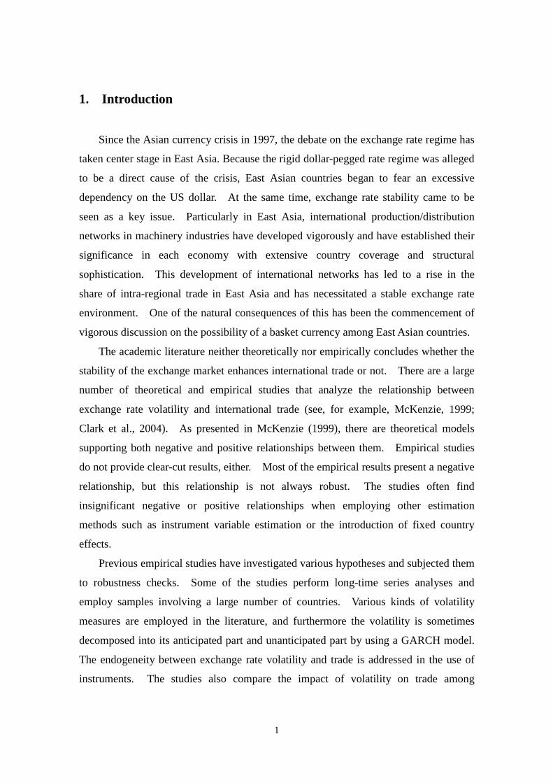
1. Introduction

Since the Asian currency crisis in 1997, the debate on the exchange rate regime has

taken center stage in East Asia. Because the rigid dollar-pegged rate regime was alleged

to be a direct cause of the crisis, East Asian countries began to fear an excessive

dependency on the US dollar. At the same time, exchange rate stability came to be

seen as a key issue. Particularly in East Asia, international production/distribution

networks in machinery industries have developed vigorously and have established their

significance in each economy with extensive country coverage and structural

sophistication. This development of international networks has led to a rise in the

share of intra-regional trade in East Asia and has necessitated a stable exchange rate

environment. One of the natural consequences of this has been the commencement of

vigorous discussion on the possibility of a basket currency among East Asian countries.

The academic literature neither theoretically nor empirically concludes whether the

stability of the exchange market enhances international trade or not. There are a large

number of theoretical and empirical studies that analyze the relationship between

exchange rate volatility and international trade (see, for example, McKenzie, 1999;

Clark et al., 2004). As presented in McKenzie (1999), there are theoretical models

supporting both negative and positive relationships between them. Empirical studies

do not provide clear-cut results, either. Most of the empirical results present a negative

relationship, but this relationship is not always robust. The studies often find

insignificant negative or positive relationships when employing other estimation

methods such as instrument variable estimation or the introduction of fixed country

effects.

Previous empirical studies have investigated various hypotheses and subjected them

to robustness checks. Some of the studies perform long-time series analyses and

employ samples involving a large number of countries. Various kinds of volatility

measures are employed in the literature, and furthermore the volatility is sometimes

decomposed into its anticipated part and unanticipated part by using a GARCH model.

The endogeneity between exchange rate volatility and trade is addressed in the use of

instruments. The studies also compare the impact of volatility on trade among

2

developed countries with that among developing countries. These studies aim to

examine the differences in the currency/exchange system, or the availability of hedging

instruments across countries, through investigating the impact of exchange rate

volatility on international trade. Recently, moreover, Clark et al. (2004)1

The fourth element is especially important in the context of East Asia. The

seminal paper in the fragmentation theory, Jones and Kierzkowski (1990), illustrates the

mechanics of fragmentation in a static setting. It claims that fragmentation of

production processes takes place when (i) production cost per se in fragmented

production blocks can be substantially reduced and (ii) service link cost for connecting

remotely located production blocks is not prohibitively high. If a reduction in

production cost by fragmentation overweighs service link cost incurred thereby, the firm

breaks apart some of its production blocks to other remote locations, so as to attain a

total cost reduction. In dynamic consideration, however, we must explicitly take into

account the cost of network set-ups and network restructuring. Apart from pure

spot-market-type transactions, transactions in production networks are relation-specific.

compared

the impact of volatility on trade in differentiated goods with that in homogenous goods.

Our study intends to contribute to the literature by clarifying differences in the

impact of exchange rate volatility among traded products or across trade structures.

Particularly in the context of East Asia, we conduct the following analysis: Firstly, we

examine whether volatility has a greater discouraging impact on trade in East Asia than

in other regions. Secondly, we try to quantify the degree to which volatility impedes

international trade in East Asia compared with tariffs and distance-related costs (e.g.,

transportation costs). Thirdly, we construct an unanticipated volatility measure

different from those used in previous literature and examine its impact on international

trade. Different from the volatility measures employed in the previous studies, this

unanticipated volatility measure is constructed by using not only the past exchange rates

but also the prospect of countries held by exchange market players (bankers). Fourthly,

we examine whether machinery parts trade is more sensitive to volatility than finished

machinery products.

1 Their finding of a larger impact on differentiated goods trade indicates that exchange rate volatility occupies a significant fraction of fixed entry costs since, from the theoretical point of view, differentiated goods trade is more sensitive to such costs.

3

Only a slight defect or delay of one single part may cause a serious malfunctioning of

the whole production system, and thus firms carefully select credible business partners

hooked up with reliable service links. Exchanges rates are one of the crucial elements

that generate uncertainty in the competitiveness of business partners as well as service

link costs. As a consequence, firms or production plants located in countries with high

volatility in exchange rates are less likely to be incorporated with production networks.

Indeed, some Japanese firms report that exchange rate stability is essential for

back-and-forth transactions of intermediate goods in international production networks

(Ito et al., 2008)2. On the other side of the coin, once production networks are in place,

transactions become stable, which suggests the existence of network restructuring cost.3

2 The Research Institute of Economy, Trade and Industry (RIETI) conducted hearings on strategies for exchange risk management with a number of Japanese machinery firms as a part of their project on “The Optimal Exchange Rate Regime for East Asia”. Ito et al. (2008) summarizes their results. 3 Obashi (2008) rigorously verifies that machinery parts and components trade in East Asia are more stable over time than machinery finished products by employing the method of the survival analysis.

There are also the previous studies with special attention on East Asia: for example,

Bénassy-Quéré and Lahrèche-Révil (2003), Poon et al. (2005), Chit el al. (2008), and

Thorbecke (2008). While these paper employs different approaches such as an

error-correction model and panel data techniques, different sample period, and different

sample countries, all these papers found the negative relationship between exports and

exchange rate volatility in East Asia. Our paper is in particular closely related to

Thorbecke (2008). He investigates how exchange rate volatility affects electronic

parts and components exports within East Asia and finds that the volatility does reduce

trade in electronic parts and components within the region. On the other hand, this

paper examines whether there are differences in the impacts of the volatility between

finished machinery goods and machinery parts. This investigation contributes to

enhancing our understanding on the mechanics of international production/distribution

networks.

The reminder of this paper is organized as follows: Section 2 explains our empirical

methodology and an overview of our volatility measure. Section 3 reports on our

regression results, and Section 4 concludes our argument.

4

2. Empirical Issues

This section offers an outline of our empirical methodology for testing the

relationship between trade and exchange volatility. Data issues and their overview

follow.

2.1. Empirical Methodology

It is well known that gravity equations can be supported by various kinds of

theoretical models. Taking advantage of this property, a large number of researchers

have performed a gravity analysis in order to carry out empirical investigations on

correlations between international trade and the variables concerned. Following the

recent literature on exchange volatility, this paper also employs a gravity equation

approach.

The baseline equation is shown by:

ln Tij = β0 +β1 ln GDPi + β2 ln GDPj + β3 ln distanceij + β4 volatilityij

+ β5 languageij + β6 adjacencyij + β7 colonyij + β8 comcolij + εij.

The time subscript t is omitted in this equation. Tij represents real export values of

country i to country j. GDPi denotes real gross domestic product in country i.4

The literature has applied various kinds of variables for exchange rate volatility,

volatilityij. In this paper, following Rose (2000), we primarily use a widely-used

indicator, the real exchange rate volatility, which is constructed as the standard

deviation of the first-difference of the monthly natural logarithm of bilateral real

distanceij is the geographical distance between countries i and j. languageij is an

indicator variable taking the value unity if a common language is spoken by at least 9%

of the population in both countries i and j, and zero otherwise adjacencyij takes the

value of one if the two countries are contiguous and zero otherwise. εij is a disturbance

term.

4 To our best knowledge, it is an irreconcilable issue which is better in gravity analyses, nominal variable or real variable. Although the real variables are employed in the reported tables, we have confirmed that the results are qualitatively unchanged even in the case of the nominal variables.

5

exchange rates in the five years preceding period t. A number of other indicators are

also introduced in our robustness checks.

We first estimate the above gravity equation for bilateral trade values in the world

by the ordinary least squares (OLS) method. Then, by introducing an East Asia

dummy interacting with the real exchange rate volatility, we examine the impact of

exchange rate volatility on trade in East Asia relative to that in the other regions. The

East Asia dummy takes the value unity if both countries i and j are East Asian countries

and zero otherwise. Next, by restricting our sample to intra-East Asian trade, we

investigate more closely the impact of exchange rate volatility on trade. By

introducing tariffs as an independent variable, we quantify the degree of significance of

the effect of exchange rate volatility on East Asian trade compared with that of tariffs.

In addition, we decompose the real exchange rate volatility into an anticipated volatility

that is predicted from economic and social conditions and an unanticipated volatility as

the residual, both of these being introduced as explanatory variables. Finally, to verify

the importance of stable transactions of intermediate goods in the formation of

production networks, we regress the gravity equation for trade in finished machinery

goods and trade in machinery parts separately.

2.2. Data Overview

Our sample includes bilateral trade between 60 countries (see Appendix) from 1992

to 2005. Data on international trade values are obtained from UN Comtrade. The HS

code list of parts and components is drawn from Ando and Kimura (2005). Data on

GDP come from the World Development Indicator (World Bank). GDP is deflated by

the U.S. wholesale price index, which is also from the World Development Indicator.

The source of distanceij, languageij, and adjacencyij is the CEPII website. The

nominal exchange rate (monthly) is drawn from IFS (af) and is deflated by the monthly

consumer price index, which is also from IFS.

Figure 1 depicts changes in the simple average of real exchange rate volatilities

among countries in each region. Large volatility is apparent in Latin America in the

first half of the 1990s. While the volatility there subsequently declined rapidly,

volatility in East Asia began to rise in 1998. As a result, by around 2000, East Asia

had the largest degree of volatility in the world. Volatility in Africa has been relatively

6

large since the first half of the 1990s, while that in Europe has been relatively small.

Figure 1. Changes in Real Exchange Rate Volatility by Region

0.00

0.02

0.04

0.06

0.08

0.10

0.12

1992

1993

1994

1995

1996

1997

1998

1999

2000

2001

2002

2003

2004

2005

Year

East Asia Europe Latin America Africa EA (Unanticipated)

Source: Authors’ calculation

In Figure 1, “unanticipated” indicates unanticipated exchange volatility in East Asia.

The unanticipated exchange volatility is constructed as follows: Firstly, we regress the

following equation by the OLS method:

volatilityij,t = α0 +α1 ln Riski,t-5 +α2 ln Riskj,t-5 + ςij, (1)

where Riski denotes country risk in country i. Secondly, by using estimates of α0, α1,

and α2, we can obtain the residual of each observation. Finally, we define the

unanticipated volatility as the absolute value of the residual. That is, the unanticipated

volatility is defined as the mass of exchange volatility not predicted by the country risk

for each of the countries. As a proxy for the country risk, we use the country risk

index, which is drawn from Institutional Investor (Institutional Investor, various issues).

This index is the aggregate of bankers’ evaluations on the risk of default, and a larger

index indicates that the country has a smaller risk of default. As shown in Figure 1,

together with the “total” volatility, the unanticipated volatility in East Asia rose from

1998. This rise seems to reflect the currency crisis.

7

3. Empirical Results In the following, we first present baseline results regarding the several hypotheses

listed in section 2.1. Following this, the results of various kinds of robustness checks

are reported.

3.1. Baseline Results

3.1.1. East Asia versus the World Countries

Table 1 reports the regression results obtained using our full sample. Columns

two and three show the values for all manufactured goods and machinery products,

respectively. Almost all coefficients are estimated to be significant with the expected

signs. Large GDP of importers and exporters, and short distances between trading

countries encourage international trade. Our main interest in this paper lies in the

results concerning the exchange rate volatility, for which coefficients are significantly

negative in both columns. The negative coefficients imply that large volatility

discourages international trade in both manufactured goods and machinery products in

the world. This result may reflect the fact that exchange rate volatility generates a

significant fraction of the fixed costs for trading activities.

The East Asian slope dummy is introduced into our equation, as shown in columns

four and five of Table 1. The results for most of the usual coefficients are unchanged

from the previous results. The slope coefficients are significantly negative, implying

that intra-East Asian trade is more seriously discouraged by exchange rate volatility

than trade in other regions. The immaturity of the international exchange market and

of hedging instruments may account for the creation of this more serious impact on East

Asia. We will observe later that, in addition to the immaturity of the financial sector,

the mechanics of machinery trade contribute to this result.

8

Table 1. Results of Full Sample Regressions

Manu Machine Manu Machineimporter's GDP 1.412*** 1.256*** 1.412*** 1.256***

[0.011] [0.010] [0.011] [0.010]exporter's GDP 2.264*** 2.238*** 2.264*** 2.238***

[0.010] [0.009] [0.010] [0.009]distance -1.203*** -1.037*** -1.203*** -1.038***

[0.045] [0.041] [0.045] [0.041]volatility -1.977*** -1.626*** -1.771*** -1.404**

[0.668] [0.611] [0.677] [0.619] * East Asia -17.390*** -18.770***

[2.377] [2.313]language 0.923*** 0.753*** 0.920*** 0.749***

[0.075] [0.069] [0.075] [0.069]adjacency -0.094 -0.013 -0.111 -0.032

[0.139] [0.130] [0.139] [0.130]colony 1.449*** 1.466*** 1.454*** 1.472***

[0.126] [0.116] [0.126] [0.116]comcol 1.562*** 1.553*** 1.560*** 1.551***

[0.103] [0.094] [0.103] [0.094]East Asia 2.669*** 3.626*** 3.316*** 4.325***

[0.095] [0.094] [0.128] [0.130]Europe 1.712*** 2.234*** 1.716*** 2.239***

[0.095] [0.088] [0.095] [0.088]Latin America 2.639*** 2.311*** 2.640*** 2.311***

[0.109] [0.098] [0.109] [0.098]Africa -0.519** -0.505** -0.517** -0.503**

[0.238] [0.208] [0.238] [0.208]Year dummy YES YES YES YESObs. 49,549 49,549 49,549 49,549R-sq 0.5837 0.6089 0.5838 0.6090

Notes: Heteroskedasticity-consistent standard errors (White) are in parentheses. ***, **, and * show 1%, 5%, and 10% significance, respectively.

3.1.2. The Impact of Unanticipated Volatility on East Asian Trade

In Table 2, we narrow down our sample to intra-East Asian trade. Looking at the

results in columns two and three, tariffs, of which data are available in the Handbook of

Statistics (UNCTAD), are introduced as an independent variable, ln (1+tariffs(%)/100),

and their coefficients are estimated to be negative. The coefficient for adjacency turns

out to be positive and significant, though that for colony is estimated to be negative.

The coefficients for exchange rate volatility are significantly negative, and their

9

magnitude is at almost the same level as that of the results in Table 1. The results in

the other variables are qualitatively unchanged from the previous ones in Table 1,

though the magnitude of the coefficients is slightly decreased.

Table 2. Regression Results for Intra-East Asian Trade Manu Machine Manu Machine Final Parts Final Parts

importer's GDP 0.539*** 0.454*** 0.310*** 0.181*** 0.601*** 0.419*** 0.319*** 0.119***[0.022] [0.029] [0.023] [0.030] [0.031] [0.032] [0.030] [0.032]

exporter's GDP 0.836*** 0.814*** 0.644*** 0.543*** 0.960*** 0.788*** 0.668*** 0.524***[0.022] [0.029] [0.021] [0.026] [0.031] [0.032] [0.030] [0.033]

distance -0.400*** -0.432*** -0.439*** -0.468*** -0.332*** -0.491*** -0.393*** -0.524***[0.047] [0.066] [0.044] [0.059] [0.076] [0.078] [0.064] [0.070]

tariffs -4.429*** -5.012*** -2.660*** -3.248***[0.515] [0.732] [0.458] [0.695]

volatility -15.960*** -20.481*** -15.783***-24.669***[1.347] [1.574] [1.858] [1.912]

unanticipated volatility -11.989*** -17.844*** -10.012***-20.582***[1.408] [1.737] [1.811] [1.974]

importer's risk 1.447*** 1.657*** 2.012*** 2.021***[0.097] [0.124] [0.129] [0.140]

exporter's risk 1.142*** 1.625*** 1.900*** 1.520***[0.092] [0.121] [0.112] [0.122]

language 0.409*** 0.559*** 0.382*** 0.503*** 0.629*** 0.623*** 0.501*** 0.542***[0.065] [0.079] [0.057] [0.067] [0.087] [0.090] [0.073] [0.080]

adjacency 0.543*** 0.403*** 0.486*** 0.364*** 0.411*** 0.216 0.371*** 0.293**[0.122] [0.134] [0.119] [0.121] [0.136] [0.140] [0.115] [0.126]

colony -0.444*** -0.249* -0.616*** -0.458*** -0.371 0.096 -0.720*** -0.215[0.094] [0.138] [0.089] [0.126] [0.244] [0.251] [0.205] [0.224]

comcol 0.927*** 0.983*** 0.463*** 0.371*** 1.464*** 1.103*** 0.638*** 0.443***[0.089] [0.109] [0.088] [0.109] [0.146] [0.150] [0.129] [0.141]

Year dummy Yes Yes Yes Yes Yes Yes Yes YesDisc (distance) 19% 22% 7% 9%Disc (tariff) 201% 251% 129% 174%Wald test (p-value)Obs. 997 997 997 997 957 957 957 957R-sq 0.7068 0.6223 0.7722 0.7124 0.6190 0.585 0.733 0.6735

0.0000 0.0000

Notes: See notes to Table 1. The null hypothesis in the Wald test states that the coefficient for volatility/unanticipated volatility between the final goods and parts equations is identical.

How large is the trade impediment caused by exchange rate volatility, compared

with other trade impediments such as tariffs? Our volatility measure is a form of

standard deviation, and thus direct interpretation of the magnitude of its coefficients is

difficult. In order to estimate its magnitude intuitively, we quantify the seriousness of

the effect of exchange rate volatility on East Asian trade, compared with the effects of

distance-related costs and tariffs, by calculating the following measures

(Discouragement):

10

)()(

)(imean

VolatilitymeaniDisc

i

volatility

⋅

⋅=

ββ

for ∈i {distance, tariffs},

where mean (i) denotes the mean value of variable i. The results are reported in the

rows, Disc (distance) and Disc (tariff). We can conclude here that exchange rate

volatility on average discourages international trade by a factor of 0.2 and has twice the

impact of distance-related costs and tariffs, respectively. The finding that exchange

rate volatility penalizes East Asian trade more seriously than one of the most

well-known impediments, tariffs, is important, even though tariffs have already been

lowered substantially in East Asia.

Columns four and five in Table 2 report regression results obtained using the

unanticipated volatility measure.5

Here we regress the gravity equation for trade in finished machinery goods and

trade in machinery parts and components separately in East Asia.

The equations in the columns also include importer

and exporter risk indices. The coefficients for both risk indices are significantly

positive, implying that the lower the risk of default in trading countries, the more

international trade occurs between them. The coefficients for unanticipated volatility

are also estimated to be significant in both columns. The negative coefficients here

indicate that, in addition to country risk, the existence of exogenous factors creating

exchange rate volatility reduces manufacturing and machinery trade. Furthermore,

unanticipated volatility on average has a slightly larger discouraging impact on trade

than tariffs. Comparing with the results in columns two and three, we conclude that a

significant portion of the negative impact of exchange rate volatility is induced by its

unanticipated part.

3.1.3. Finished Goods Trade versus Intermediate Goods Trade

6

5 Exporters would predict future volatility by using a lot more information. To examine the impact of more purely random shocks in exchange rates, we also estimated the expected volatility by introducing not only country risk but also fixed importer and exporter effects and year dummies. But, the results were qualitatively unchanged. 6 The tariff rates are dropped from the regression equations because the ready-made tariff data are not available for machinery final goods and machinery parts separately.

To formally test

whether exchange rate volatility has a different impact on finished products and parts,

we conduct the Wald test using the null hypothesis, which states that the coefficients are

11

identical in both equations. These results are reported in columns six to nine in Table

2.

There are three points to note. First, as above, standard gravity variables such as

GDPs are estimated with the expected signs. Second, coefficients for total volatility

and unanticipated volatility are again significantly negative. Exchange rate volatility is

a significant impediment to trade in both finished machinery goods and machinery parts.

Third, and most interestingly, the Wald tests reject the null hypothesis at the 1% level of

significance. This implies that trade in machinery parts is more sensitive to exchange

rate volatility than trade in finished machinery goods, which indicates that stable

transactions of parts are crucial to the formation of production networks.

3.1.4. Simulation Analyses

Here we perform simple simulation analyses by using the results in Table 2. We

simulate the average growth of exports by an East Asian country by reducing its sample

mean level of real exchange rate volatility (0.037) to the ECU level and the EURO level.

The mean level in the ECU countries during the period 1992-1998 (0.019) is used as the

ECU level, and that in the EURO countries during the period 1999-2005 (0.010) as the

EURO level. Although those levels are not necessarily achieved only by the

introduction of the ECU and EURO, we simply apply those levels for East Asia, which

can possibly be interpreted as the effect of introducing an East Asian basket currency or

an East Asian common currency, respectively. The case of complete elimination of

mean volatility in East Asia (0.037) is also simulated. These hypothetical scenarios are

compared with the case of a complete reduction of the sample means for tariffs (0.066

for manufacture; 0.060 for machinery).

The simulation results are reported in Table 3. For example, the simulation result

of “ECU” in “Manu” is derived from the following calculation: 100*[exp((0.019 –

0.037) * (-15.960)) - 1] %. “-15.960” is the estimate of volatility shown in column two

of Table 2. In all scenarios, the magnitude of the effects is not small at all. The

introduction of a common currency almost doubles machinery exports. In the case of

complete elimination of exchange rate volatility, which would be impossible in the real

world though, the increase in machinery exports is more than twice. In addition, an

introduction of a common currency has a larger impact than the achievement of free

12

trade (zero tariffs). We can thus conclude that the introduction of a basket currency or

a common currency would substantially contribute to enhancing the magnitude of

international trade in East Asia.

Table 3. Simulation: Rise of Exports in Each East Asian Country

Manu Machine Final PartsECU 33% 44% 24% 37%EURO 54% 74% 38% 62%ALL 81% 114% 56% 94%Tariffs 34% 35%

Notes: The simulation scenario involves the reduction of exchange rate volatility to its level in ECU countries and in EURO countries respectively. In addition, the simulation result of complete elimination of mean volatility in East Asia is also reported (ALL). The mean of volatility in ECU countries (92-98) and EURO countries (99-05) is 0.0194559 and 0.0101294, respectively. The mean of volatility in East Asia (92-05) is 0.037187.

3.2. Robustness Checks

In almost all previous studies, the negative effect of exchange rate volatility on

trade is not found to be robust, which is quite contrary to our results. To confirm our

strong results, we perform various kinds of robustness checks, which are reported in

Tables 4 to 7.

Firstly, in Tables 4 and 5, we introduce importer-year and exporter-year dummy

variables in order to control time-variant country-specific characteristics. In this

specification, the effects of multilateral resistance terms, which is one of the serious

issues in gravity analysis, are also controlled. With our full sample (Table 4), the

coefficients for volatility are still negatively significant. However, those for East Asia

slope dummy turn out to be insignificant while those are still negatively estimated. In

East Asian sample (Table 5), moreover, volatility coefficients themselves are not

significant. As a result, controlling time-variant country-specific elements, e.g., the

immaturity of international exchange market and hedging instruments, in each East

Asian country, we cannot observe the significant negative impacts of exchange rate

volatility in East Asia. To put it the other way around, we can say that the sources of

its negative impacts in East Asia are time-variant country-specific elements. In

addition, the absolute magnitude of the volatility coefficient is larger in parts equation,

13

though that is insignificant in both equations and the Wald test does not reject the null

hypothesis.

Table 4. Robustness Checks of Full Sample Regression: Importer-year and Exporter-year Dummies

Manu Machine Manu Machinedistance -1.922*** -1.686*** -1.922*** -1.686***

[0.043] [0.039] [0.043] [0.039]volatility -8.495*** -6.293*** -8.533*** -6.365***

[2.730] [2.412] [2.734] [2.416] * East Asia -1.761 -3.315

[2.498] [2.193]language 1.026*** 0.822*** 1.026*** 0.821***

[0.067] [0.060] [0.067] [0.060]adjacency -0.260** -0.059 -0.262** -0.062

[0.116] [0.102] [0.116] [0.102]Colony 0.874*** 1.070*** 0.874*** 1.071***

[0.099] [0.086] [0.099] [0.086]Comcol 0.300*** 0.515*** 0.300*** 0.516***

[0.096] [0.086] [0.096] [0.086]East Asia -2.027*** -1.154*** -1.961*** -1.031***

[0.108] [0.098] [0.145] [0.130]Europe -1.782*** -1.088*** -1.782*** -1.089***

[0.094] [0.083] [0.094] [0.083]Latin America 2.223*** 2.046*** 2.224*** 2.047***

[0.126] [0.111] [0.127] [0.111]Africa 1.871*** 1.791*** 1.872*** 1.792***

[0.205] [0.178] [0.205] [0.178]Importer-year dummy Yes Yes Yes YesExporter-year dummy Yes Yes Yes YesObs. 49,549 49,549 49,549 49,549R-sq 0.7832 0.8129 0.7832 0.8129 Note: See notes to Table 1.

14

Table 5. Robustness Checks of East Asian Sample Regression: Importer-year and Exporter-year Dummies

Manu Machine Final Partsdistance -0.371*** -0.324*** -0.270*** -0.393***

[0.044] [0.047] [0.039] [0.040]volatility -4.015 -2.046 -1.400 -4.139

[3.461] [3.458] [3.011] [3.023]language 0.199*** 0.424*** 0.362*** 0.468***

[0.059] [0.062] [0.057] [0.057]adjacency 0.607*** 0.565*** 0.588*** 0.516***

[0.136] [0.146] [0.084] [0.084]Colony -0.466*** -0.362*** -0.454*** -0.376***

[0.096] [0.100] [0.127] [0.128]Comcol 0.364*** 0.295*** 0.426*** 0.278***

[0.073] [0.079] [0.084] [0.084]Importer-year dummy Yes Yes Yes YesExporter-year dummy Yes Yes Yes YesWald test (p-value)Obs. 997 997 957 957R-sq 0.8917 0.9101 0.9108 0.9074

0.2912

Note: See notes to Table 2.

Secondly, to further explore volatility measures, we attempt to employ two kinds of

volatility measures: GARCH volatility and nominal volatility. In the subsequent

regressions, we restrict our sample to East Asia. By following Clark et al. (2004), the

former is the conditional volatilities of the exchange rates estimated using a GARCH

(1,1), and the underlying equation for the model is an ARIMA (0,1,0) process of the log

of real exchange rates. The last estimated conditional standard deviation of each

country pair is used as the approximation of the conditional volatility at the beginning

of next period.7

7 For instance, the conditional volatility of 2000 equals the estimated conditional standard deviation for December 1999 in the GARCH regressions.

The latter is the standard deviation of the first-difference of the

monthly natural logarithm of bilateral nominal exchange rates in the five years

preceding period t. The results are reported in Table 6. Similar to Tables 4 and 5,

time-variant country characteristics are controlled. However, contrary to them, there

are the estimators of volatility coefficients to be negatively significant at ten percent

level. Thus, we can conclude that, in some volatility measures, the source of the

negative impacts of exchange volatility still remains even if we control time-variant

country characteristics.

15

Table 6. Robustness Checks of East Asian Sample Regression: Two Volatility Measures

Manu Machine Final Parts Manu Machine Final Partsdistance -0.369*** -0.326*** -0.270*** -0.394*** -0.378*** -0.329*** -0.276*** -0.398***

[0.043] [0.046] [0.039] [0.039] [0.044] [0.048] [0.040] [0.040]GARCH volatility -2.489 -2.793 -1.321 -4.136*

[2.393] [2.384] [2.161] [2.168]volatility (nominal) -5.887* -3.48 -3.965 -4.961*

[3.448] [3.441] [2.844] [2.856]language 0.196*** 0.420*** 0.360*** 0.463*** 0.201*** 0.425*** 0.362*** 0.469***

[0.059] [0.062] [0.057] [0.057] [0.059] [0.062] [0.057] [0.057]adjacency 0.633*** 0.573*** 0.595*** 0.538*** 0.581*** 0.547*** 0.559*** 0.501***

[0.129] [0.136] [0.080] [0.080] [0.139] [0.150] [0.085] [0.085]colony -0.483*** -0.385*** -0.464*** -0.409*** -0.475*** -0.368*** -0.462*** -0.383***

[0.097] [0.101] [0.129] [0.129] [0.096] [0.100] [0.127] [0.128]comcol 0.367*** 0.291*** 0.425*** 0.276*** 0.360*** 0.292*** 0.420*** 0.277***

[0.073] [0.078] [0.084] [0.084] [0.073] [0.078] [0.083] [0.084]Importer-year dummy YES YES YES YES Yes Yes Yes YesExporter-year dummy YES YES YES YES Yes Yes Yes YesWald test (p-value)Obs. 997 997 957 957 997 997 957 957R-sq 0.8916 0.9102 0.9108 0.9075 0.8920 0.9102 0.9109 0.9075

GARCH Volatility Nominal Volatility

0.1306 0.6848

Note: See notes to Table 2.

Finally, here we regress the first-difference logarithmic form of the gravity equation

with time-variant importer and exporter dummy variables. In this paper, as in almost

all gravity studies, we have completely disregarded potential stationarity issues. If our

variables are integrated of order one, such a first-difference logarithmic form of the

gravity equation would be appropriate. In the equation, to control effects of exchange

rate changes per se on trade, we introduce the first-difference logarithm of real

exchange rates between trading countries: the larger this variable is, the more rapidly

the exporter’s currency is devaluated.8

8 To assure comparability, we introduced the percentage change in exchange rates. The internationally comparable exchange rates are available in the CEPII-CHELEM database.

The results are reported in Table 7. The

coefficients for exchange rate change have significantly positive sign in manufacturing

and parts equations. The coefficients for volatility change are no longer estimated to

be significantly negative. Notice that not only time-variant country characteristics but

also time-invariant country pair characteristics are controlled in these regression

equations. Thus, we can say that time-variant pair elements are not a significant part

of the negative impacts of exchange volatility on trade, though we cannot well interpret

16

the positive coefficients.9

Manu Machine Final Partsexchange rate change 0.208*** -0.078 -0.155 0.640***

[0.078] [0.092] [0.149] [0.085]volatility change -4.088 -1.333 5.268** 4.095**

[7.433] [7.383] [2.565] [1.968]Importer-year dummy Yes Yes Yes YesExporter-year dummy Yes Yes Yes YesWald test (p-value)Obs. 936 936 885 885R-sq 0.0394 0.0458 0.5723 0.6498

0.6961

Table 7. Robustness Checks on East Asian Sample Log-difference Regression: Exchange Rate

Note: See notes to Table 2.

4. Concluding Remarks

In this paper, we empirically investigated the relationship between exchange rate

volatility and trade, focusing on East Asia. Our findings are summarized as follows:

first, intra-East Asian trade is discouraged by exchange rate volatility more seriously

than trade in other regions. Second, one important source for the discouragement is

that intermediate goods trade in international production networks, which is quite

sensitive to exchange rate volatility compared with other types of trade, occupies a

significant fraction of East Asian trade. Third, the negative effect of the volatility is

greater than that of tariffs and smaller than that of distance-related costs in East Asia.

Fourth, the sources of such negative impacts of the volatility are time-variant

country-specific elements. Last, our simulation analysis shows that the introduction of

a basket currency or a common currency would have a larger positive impact on

international trade than free trade.

In interpreting our results, we may need to consider a link between the reduction of

exchange rate volatility and foreign direct investment (FDI). Kiyota and Urata (2004)

9 Conducting dynamic least squares as a further robustness check, we obtain basically the same results.

17

show a significant negative relationship between exchange rate volatility and Japanese

FDI to East Asian countries. The introduction of an East Asian basket currency or an

East Asian common currency may induce a substantial increase in international goods

trade, together with a further encouragement of FDI in East Asia.

18

Appendix. Sample Countries Region CountryAfrica Algeria, Ghana, Kenya, Madagascar, Mauritius, Morocco, Senegal, SeychellesEast Asia China, Hong Kong, Indonesia, Japan, Korea, Malaysia, Philippines, Singapore, ThailandEurope

Latin America

Others

Austria, Denmark, Finland, France, Greece, Hungary, Iceland, Italy, Malta, Netherlands, Norway,Portugal, Spain, Sweden, Switzerland, United KingdomArgentina, Barbados, Bolivia, Brazil, Chile, Colombia, Costa Rica, El Salvador, Guatemala,Honduras, Jamaica, Mexico, Panama, Paraguay, St.Lucia, Trinidad and TobagoCanada, United States, Fiji, Cyprus, India, Israel, Jordan, Nepal, Pakistan, Saudi Arabia, SriLanka

19

References

Ando, M., Kimura, F., 2005. The formation of international production and distribution networks in East Asia. In: Ito, T. and Rose, A. (Eds.). International Trade in East Asia, Chicago: University of Chicago Press: 177-213.

Bénassy-Quéré, A., Lahrèche-Révil, A., 2003. Trade linkages and exchange rates in Asia: The role of China. Working paper No. 2003-21, CEPII.

Chit, M., Rizov, M., Willenbockel, D, 2008. Exchange rate volatility and exports: New empirical evidence from the emerging East Asian Economies. Middlesex University Economics and Statistics Discussion Paper No. 127.

Clark, P., Tamirisa, N., Wei, S., Sadikov, A., Zeng, L., 2004. A new look at exchange rate volatility and trade flows. International Monetary Fund, Washington DC, Occasional Paper, No. 235.

Ito, T., Koibuchi, S., Sasaki, Y., Sato, K., Shimizu, J., Hayakawa, K., Yoshimi, T., 2008. Choice of invoice currency and exchange risk management: Case studies of Japanese firms. RIETI Discussion Paper Series 08-J-009 (in Japanese).

Jones, R. W., Kierzkowski, H., 1990. The role of services in production and international trade: a theoretical framework. In: Jones, R. W. and Krueger, A. O. (Eds.). The Political Economy of International Trade: Essays in Honor of R. E. Baldwin, Oxford: Basil Blackwell.

Kiyota, K., Urata, S., 2004. Exchange rate, exchange rate volatility and foreign direct investment. The World Economy 27(10), 1501-1536.

McKenzie, M., 1999. The impact of exchange rate volatility on international trade flows. Journal of Economic Surveys 13(1), 71-106.

Obashi, A., 2008. Stability of production networks in East Asia: duration and survival of trade. mimeo.

Poon, W., Choong, C., M. Habibullah, M., 2005. Exchange rate volatility and export for selected East Asian countries: Evidence from error-correction model. ASEAN Economic Bulletin 22(2), 144–159.

Rose, A., 2000. One money, one market: The effect of common currencies on trade. Economic Policy, April, 9-45.

Thorbecke, W., 2008. The effect of exchange rate volatility on fragmentation in East Asia: Evidence from the electronics industry. Journal of the Japanese and International Economies 22(4), 535-544.

ERIA Discussion Paper Series

No. Author(s) Title Year

2009-02 Fukunari KIMURA The Spatial Structure of Production/Distribution Networks and Its Implication for Technology Transfers and Spillovers

Mar 2009

2009-01 Fukunari KIMURA and Ayako OBASHI

International Production Networks: Comparison between China and ASEAN

Jan 2009

2008-03 Kazunobu HAYAKAWA and Fukunari KIMURA

The Effect of Exchange Rate Volatility on International Trade in East Asia

Dec 2008

2008-02

Satoru KUMAGAI, Toshitaka GOKAN, Ikumo ISONO, and Souknilanh KEOLA

Predicting Long-Term Effects of Infrastructure Development Projects in Continental South East Asia: IDE Geographical Simulation Model

Dec 2008

2008-01

Kazunobu HAYAKAWA, Fukunari KIMURA, and Tomohiro MACHIKITA

Firm-level Analysis of Globalization: A Survey Dec 2008