THE EFFECT OF DRIVE SIGNAL LIMITING ON HIGH CYCLE FATIGUE LIFE ANALYSIS

Frédéric Kihm1*and Stephen A. Rizzi2

1HBM-nCode Products Division Technology Center, Brunel Way, Catcliffe Rotherham, S60 5WG, UK E-mail: frederic.kihm@hbmncode.com 2NASA Langley Research Center Aeroacoustics Branch Hampton, Virginia 23681 USA E-mail: Stephen.A.Rizzi@nasa.gov Keywords: Fatigue, sigma clipping, random shaker tests, non-Gaussian.

ABSTRACT It is common practice to assume a Gaussian distribution of both the input acceleration and the response when modeling random vibration tests. In the laboratory, however, shaker controllers often limit the drive signal to prevent high amplitude peaks. The high amplitudes may either be truncated at a given level (so-called brick wall limiting or abrupt clipping), or compressed (soft limiting), resulting in drive signals which are no longer Gaussian. The paper first introduces several methods for limiting a drive signal, including brick wall limiting and compression. The limited signal is then passed through a linear time-invariant system representing a device under test. High cycle fatigue life predictions are subsequently made using spectral fatigue and rainflow cycle counting schemes. The life predictions are compared with those obtained from unclipped input signals. Some guidelines are provided to help the test engineer decide how clipping should be applied under different test scenarios.

1. INTRODUCTION During vibration shaker testing, the controller typically limits the drive signal to prevent high amplitude peaks from damaging shaker components. Limiting therefore allows the shaker system to deliver more power, because it can represent random signals of greater RMS power by eliminating the rare high amplitude peaks. Because the high amplitudes are removed above a given level, the resulting limited signal is no longer Gaussian. So, the crucial question is: “What is the influence of limiting the drive signal on the fatigue life of a specimen during a random shaker test?”

In a recent study [1], some tests were performed on a specimen, instrumented with an accelerometer and strain gages. The drive signal was limited at various levels using two methods. In the first method, high amplitudes were truncated at a given level. This approach is commonly referred to as brick wall limiting or abrupt clipping. In the second method, high amplitude peaks are compressed using a nonlinear weighting function such that no peaks

exceed a prescribed level. This approach is commonly referred to as compression or soft clipping. The time domain signals of the drive and the responses were recorded. It was shown that the response signals were not clipped and tended towards Gaussian.

This paper studies the effect of drive signal limiting using simulated data. The drive signal and theoretical response characteristics are first considered. Data from numerical simulations are then used to validate the response prediction and make fatigue damage estimates using frequency domain (spectral fatigue) and time domain (rainflow cycle counting) schemes. Finally, some guidelines are offered to help determine how clipping should be applied under different test scenarios.

2. LIMITING THE EXCITATION SIGNAL 2.1 Brick wall limiting – Abrupt clipping

Brick wall limiting or abrupt clipping is a technique that simply cuts off the peaks at a given level. The resulting signal is therefore non-Gaussian. Abrupt clipping directly influences the resulting signal’s crest factor, b, which is defined as the maximum value divided by the RMS of the signal. The maximum value reached by a clipped signal is denoted as xth.

Although very easy to implement, using either analog or digital means, abrupt clipping introduces strong high frequency distortion in the resulting spectrum [2].

The probability density function (PDF) of an abruptly clipped signal shows peaks in its extremities, as illustrated in Figure 1. These peaks are localized at the level where the abrupt clipping occurs (xth = ±6g).

Figure 1: PDF of a brick wall limited signal (solid) versus a Gaussian signal (dashed).

The PDF of an abrupt clipped signal can be expressed as:

Abrupt_Clipped

( )

1PDF 12 2

0

th

thth

x

th

f x if x x

xerf if x x

if x x

σ

<

= − =

>

(1)

where f(x) is the PDF of a centered Gaussian distribution with standard deviation xσ . It can be verified that the area under the abrupt clipped PDF equals 1.0. The obtained PDF is even

and therefore the 1st and 3rd central moments are zero, giving zero mean µ and skewness λ . The root-mean-square (RMS) is then equal to the standard deviation.

The 2nd and 4th central moments, M2 and M4, of the abrupt clipped signal can be calculated from the definition of the moments of a probability distribution. The probability distribution of the abrupt clipped signal is given in equation (1). The obtained expressions for M2 and M4 are then:

21

22 2 22

2(1 )2 2

bx

bM b b erf beσπ

− = + − −

(2)

21

24 4 4 24

2(3 ) ( 3)2 2

bx

b bM b b erf e bσπ

− = + − − +

(3)

The 2nd central moment is the variance and the kurtosis κ is related to the 2nd and 4th moments as:

42

2

MM

κ = . (4)

2.2 Compression– Soft clipping Compression, or soft clipping, is an alternate way of limiting a signal. The main advantage of compression is to reduce the high frequency distortion. Different compression techniques exist.

One simple way is to use a logistic sigmoid function such as the hyperbolic tangent tanh, the arctangent arctan or the error function erf to limit the amplitudes of a Gaussian signal. In this work, the hyperbolic tangent tanh was used as the nonlinear zero-memory transformation of a Gaussian random variable x with standard deviation σx into a non-Gaussian process, according to:

tanhxx

xz bb

σσ

=

(5)

Another way to clip a signal is to modify its phase. The principle is simple; when the

inverse DFT is applied to a spectrum whose phase is random and uniformly distributed between ±π, then this will lead to a Gaussian signal. If the phase is distributed differently, the resulting signal will still exhibit the same RMS but will no longer be Gaussian. Such phase manipulation techniques are typically used by shaker controllers as they integrate well with their FFT-based algorithms [3-5]. Such a phase modification algorithm will typically lead to a sigmoid type of input-output cross plot.

Applying the PDF transform [6-9] leads to the following expressions for the PDF of a compressed signal:

( )2 22 atanh ( / )

2Compressed

1 12 1PDF

0

bthx x

thx th

th

e if x xx x

if x x

πσ− ≤ −=

>

(6)

It can be verified that the area under the PDF of a compressed signal equals 1.0. As for the abrupt clipped signal, the obtained PDF is even and therefore, the 1st and 3rd central moments are zero. The 2nd and 4th central moments, M2 and M4, can be calculated via numerical integration of expression (6). An example PDF for a compressed signal showing reduced tails is illustrated in Figure 2.

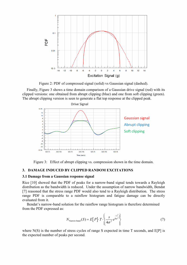
Figure 2: PDF of compressed signal (solid) vs Gaussian signal (dashed).

Finally, Figure 3 shows a time domain comparison of a Gaussian drive signal (red) with its clipped versions: one obtained from abrupt clipping (blue) and one from soft clipping (green). The abrupt clipping version is seen to generate a flat top response at the clipped peak.

Figure 3: Effect of abrupt clipping vs. compression shown in the time domain.

3. DAMAGE INDUCED BY CLIPPED RANDOM EXCITATIONS 3.1 Damage from a Gaussian response signal Rice [10] showed that the PDF of peaks for a narrow-band signal tends towards a Rayleigh distribution as the bandwidth is reduced. Under the assumption of narrow bandwidth, Bendat [7] reasoned that the stress range PDF would also tend to a Rayleigh distribution. The stress range PDF is comparable to a rainflow histogram and fatigue damage can be directly evaluated from it.

Bendat’s narrow-band solution for the rainflow range histogram is therefore determined from the PDF expressed as:

[ ]2

28Narrow-band 2( )

4

ssN S E P T e σ

σ

− = ⋅ ⋅

(7)

where N(S) is the number of stress cycles of range S expected in time T seconds, and E[P] is the expected number of peaks per second.

More generic distributions of peaks exist for wideband processes. Rice [10] showed that for a signal of arbitrary bandwidth, the PDF of peaks could be obtained from the weighted sum of the Rayleigh and Gaussian distributions. Lalanne [11] reasoned that over a sufficiently long period of time, the PDF of rainflow ranges would tend to the PDF of peaks. The Lalanne/Rice formula is given as:

[ ]2 2

2 2 22

8 (1 ) 8Wide-band 2

11( ) 12 42 8(1 )

s ss sN S E P T e e erfσ γ σγ γ γσ σπ σ γ

− −−

− = ⋅ ⋅ + + − (8)

where γ is the irregularity factor as proposed by Rice [10]. It is defined as the ratio of the number of zero up-crossings in a time signal to the number of peaks. The irregularity factor tends to 1.0 for narrow-band signals and to 0.0 in a wideband case.

The damage caused by each cycle is calculated with reference to the fatigue life curve, in this case an S-N curve similar to those illustrated in Figure 14. The S-N curve shows the number of cycles to failure, Nf, for a given stress range, S. The damage at a given stress range S is obtained as the ratio of the actual cycles contained in the rainflow histogram, to the number of cycles required to fail the component at this stress range level. The total damage is obtained by summing the damage from each individual level of stress range using the Palmgren-Miner rule [12, 13] and is expressed as:

( )( )f

N SAccumulated DamageN S

= ∑ (9)

where N(S) is the number of cycles with a particular stress range S, and Nf(S) is the number of cycles to failure for that stress range. The ratio is summed over all stress range levels. The accumulated damage is expressed as a proportion of the damage required to fail the component. Therefore the fatigue life for the component can be estimated as:

( )( )

secondsseconds

DurationFatigue Life

Accumulated Damage≅ (10)

For more details about time domain or spectral fatigue, the reader is referred to Halfpenny [14] or Lalanne [11].

3.2 Damage from a non-Gaussian response signal Winterstein [15] proposed a monotonic function g acting as a zero-memory nonlinear system to model hardening responses, that is, platykurtic responses with kurtosis < 3. It uses Hermite polynomials to approach a non-Gaussian distribution and is perfectly suited for mild deviations from a normal law. In the case of a symmetric, standardized process X, the transformation is:

34 4( ) 3g X X h X h X= − + (11)

with 4 ( 3) / 24h κ= − . The stress range S can be written in terms of peaks, P, and valleys, V, as S = P – V. In the

case of a narrow-band process, P = -V and therefore S can be rewritten as S = 2P. The nonlinear monotonic function g applies to the peaks and troughs of the process, therefore the range of the platykurtic process can be written Sc=g(P) – g(V) = 2g(P) = 2g(S/2).

The solution for the rainflow range histogram in the case of a mild non-Gaussian process can therefore be written by replacing the stress range S with 2g(S/2) in equations (7) or (8). For example, in the case of a narrow-band response, the rainflow range histogram is expressed as:

[ ] ( ) ( )2

22

2Non-Gaussian Narrow-band 2

2( )

2

g sg sN S E P T e σ

σ

− = ⋅ ⋅

(12)

4. NUMERICAL SIMULATIONS The response stress and fatigue damage for a simple, but realistic, engineering structure is next considered to demonstrate how these quantities change when the excitation loading is clipped.

4.1 The Finite Element model, boundary conditions and material properties The engineering structure considered is an off-the-shelf automotive horn bracket. The finite element model of the bracket is shown in Figure 4. The bracket was modelled with the finite element analysis program ABAQUS [16]. The bracket is constructed with 168 S3R and 5382 S4R shell elements. Two lumped masses representing the horns were constructed with 8074 C3D4 constant stress tetrahedron solid elements. Different mass values can simulate asymmetry of the weight distribution. The bracket was constructed from carbon steel, with the properties indicated in Table 1.

Under simulated test, the specimen is clamped to the test rig at the left end and excited in the transverse direction, as shown in Figure 4. The following section describes the applied loading.

Figure 4: The finite element model of the bracket with boundary conditions.

Property Value

Mechanical properties

Young Modulus 210 GPa Density 7890 kg/m3 Modal damping 0.025 Yield Stress 400 MPa Ultimate tensile strength 700 MPa

Table 1: Material properties of horn bracket.

4.2 Input signal generation The prescribed acceleration power spectral density (PSD), shown in Figure 5, originates from MIL-STD-810F [17]. The loading has a frequency range of 1-100 Hz and a scaled amplitude of 3.1g RMS.

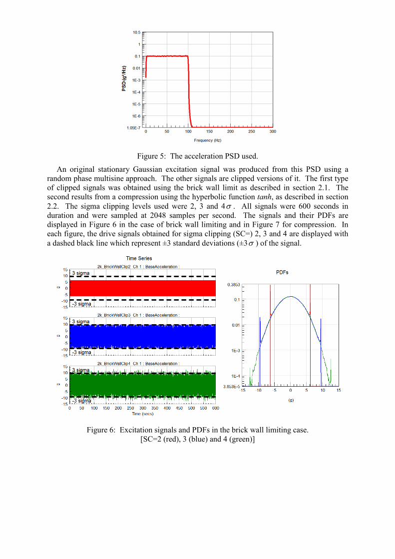
Figure 5: The acceleration PSD used.

An original stationary Gaussian excitation signal was produced from this PSD using a random phase multisine approach. The other signals are clipped versions of it. The first type of clipped signals was obtained using the brick wall limit as described in section 2.1. The second results from a compression using the hyperbolic function tanh, as described in section 2.2. The sigma clipping levels used were 2, 3 and 4σ . All signals were 600 seconds in duration and were sampled at 2048 samples per second. The signals and their PDFs are displayed in Figure 6 in the case of brick wall limiting and in Figure 7 for compression. In each figure, the drive signals obtained for sigma clipping (SC=) 2, 3 and 4 are displayed with a dashed black line which represent ±3 standard deviations (±3σ ) of the signal.

Figure 6: Excitation signals and PDFs in the brick wall limiting case.

[SC=2 (red), 3 (blue) and 4 (green)]

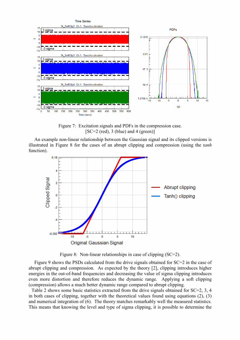
Figure 7: Excitation signals and PDFs in the compression case.

[SC=2 (red), 3 (blue) and 4 (green)]

An example non-linear relationship between the Gaussian signal and its clipped versions is illustrated in Figure 8 for the cases of an abrupt clipping and compression (using the tanh function).

Figure 8: Non-linear relationships in case of clipping (SC=2).

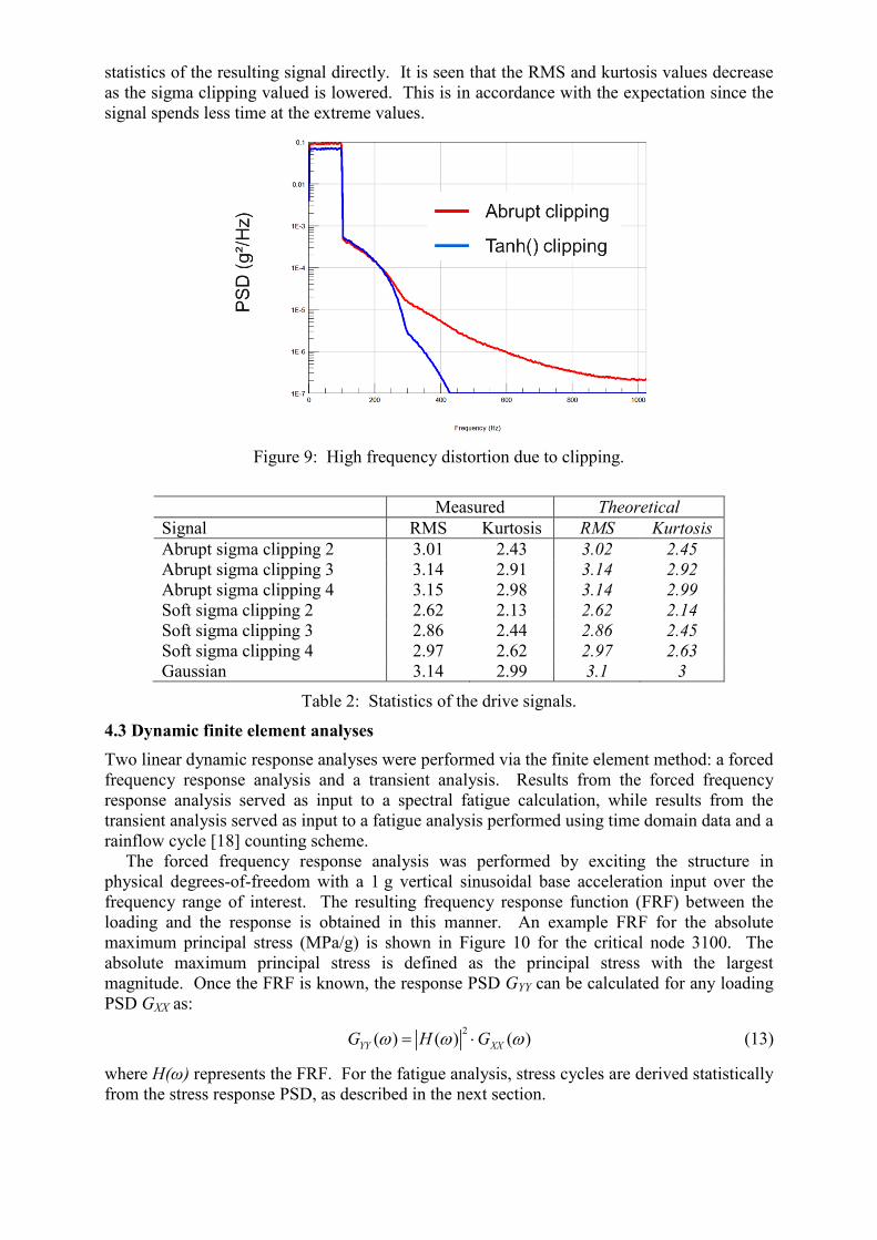
Figure 9 shows the PSDs calculated from the drive signals obtained for SC=2 in the case of abrupt clipping and compression. As expected by the theory [2], clipping introduces higher energies in the out-of-band frequencies and decreasing the value of sigma clipping introduces even more distortion and therefore reduces the dynamic range. Applying a soft clipping (compression) allows a much better dynamic range compared to abrupt clipping.

Table 2 shows some basic statistics extracted from the drive signals obtained for SC=2, 3, 4 in both cases of clipping, together with the theoretical values found using equations (2), (3) and numerical integration of (6). The theory matches remarkably well the measured statistics. This means that knowing the level and type of sigma clipping, it is possible to determine the

statistics of the resulting signal directly. It is seen that the RMS and kurtosis values decrease as the sigma clipping valued is lowered. This is in accordance with the expectation since the signal spends less time at the extreme values.

Figure 9: High frequency distortion due to clipping.

Measured Theoretical Signal RMS Kurtosis RMS Kurtosis Abrupt sigma clipping 2 3.01 2.43 3.02 2.45 Abrupt sigma clipping 3 3.14 2.91 3.14 2.92 Abrupt sigma clipping 4 3.15 2.98 3.14 2.99 Soft sigma clipping 2 2.62 2.13 2.62 2.14 Soft sigma clipping 3 2.86 2.44 2.86 2.45 Soft sigma clipping 4 2.97 2.62 2.97 2.63 Gaussian 3.14 2.99 3.1 3

Table 2: Statistics of the drive signals.

4.3 Dynamic finite element analyses Two linear dynamic response analyses were performed via the finite element method: a forced frequency response analysis and a transient analysis. Results from the forced frequency response analysis served as input to a spectral fatigue calculation, while results from the transient analysis served as input to a fatigue analysis performed using time domain data and a rainflow cycle [18] counting scheme.

The forced frequency response analysis was performed by exciting the structure in physical degrees-of-freedom with a 1 g vertical sinusoidal base acceleration input over the frequency range of interest. The resulting frequency response function (FRF) between the loading and the response is obtained in this manner. An example FRF for the absolute maximum principal stress (MPa/g) is shown in Figure 10 for the critical node 3100. The absolute maximum principal stress is defined as the principal stress with the largest magnitude. Once the FRF is known, the response PSD GYY can be calculated for any loading PSD GXX as:

2( ) ( ) ( )YY XXG H Gω ω ω⋅= (13)

where H(ω) represents the FRF. For the fatigue analysis, stress cycles are derived statistically from the stress response PSD, as described in the next section.

Figure 10: Stress FRF obtained at a critical node (3100).

For the time domain approach, a modal transient analysis was performed in ABAQUS to determine the modal response time histories for each loading condition. Stress time histories were obtained by modal superposition of the modal stresses with the modal coordinates using the commercial software nCode DesignLifeTM. This approach allowed the size of the finite element result file to be kept small, since stress time histories at all nodes are not required, and those of interest can be generated quickly. The accuracy of the modal approach is dependent on the number of modes included in the analysis. In this study, the first 5 modes were used, covering natural frequencies up to 100 Hz. This selection was made based on the FRF at the critical node, shown in Figure 10, where it is seen that the main excited modes are all within the 0-100 Hz range.

5. RESULTS 5.1 Influence of clipping on the responses The signals collected at various nodes or elements represent the responses to the clipped input. The responses are a filtered version of the input and are a result of the dynamics of the system. Thus the responses may not have the same characteristics as the input. The objective of this section is to evaluate the impact of sigma clipping on the responses.

The time domain responses to clipped (SC=2.0) inputs were collected at the critical node 3100 for both the abrupt limiting (red) and compression (blue) and are presented in Figure 11, where the dashed black lines correspond to the ± 3σ levels.

Figure 11: Stress responses at node 3100 for two types of clipping.

The ±3σ level is exceeded in all cases, even though a low sigma clipping of 2 was applied to the input. Table 3 shows the basic statistics for the strain response at the critical node for both the brick wall limiting and compression. The last column contains the theoretical output kurtosis [1, 9] calculated from:

( )

( ) ( )224

2 423.0 3.0ii

y xii

cfcf

κ κ= − +∑∑∑∑

. (14)

Here, the output kurtosis yκ is specified in terms of a non-spectrally flat noise with input kurtosis xκ , ci are the values of the autocorrelation function of the input noise, and fi are the values of the convolution of the autocorrelation function with the system impulse response function. The theory indicates the correct trends but the values do not exactly match those from the simulations. This is due to the fact that the theory considers the kurtosis of a Gaussian process to be 3.0, whereas in the present case the kurtosis of the 600 seconds signal was 2.97. A better match is obtained when correcting the theoretical output kurtosis by specifying the actual input kurtosis. This amounts to subtracting 0.03 from theoretical values shown.

From Figure 11 and Table 3, it is clear that sigma clipping applied on the input is not identically reproduced on the output signals. PDFs were calculated from the responses obtained from the various control signals obtained with SC=2, 3 and 4 and none showed truncated tails like those on the excitation as in Figure 6 and Figure 7.

Signal RMS Crest Factor Kurtosis Theoretical Kurtosis

Abrupt sigma clipping 2 48.25 5.00 2.952 2.974 Abrupt sigma clipping 3 50.31 5.13 2.967 2.995 Abrupt sigma clipping 4 50.42 5.14 2.968 2.999 Soft sigma clipping 2 41.98 4.91 2.946 2.960 Soft sigma clipping 3 45.9 5.00 2.954 2.974 Soft sigma clipping 4 47.67 5.06 2.959 2.983 Gaussian 50.42 5.14 2.970 3.000

Table 3: Statistics of the strain response.

Finally, note that the generally lower RMS response levels for the soft sigma clipping (relative to abrupt clipping and Gaussian responses) are a reflection of the lower RMS level of those inputs (see Table 2). This is consistent with the manner in which soft clipping is typically implemented on shaker controller systems. As a consequence, lower fatigue damage is to be expected.

5.2 Influence of clipping on the fatigue life The fatigue life of a component is primarily dependent on the stress or strain amplitude response at critical failure locations. The rainflow cycle counting algorithm enables a time varying stress or strain to be reduced into its fatigue cycles, where each cycle has a range and a mean. Figure 12 shows the stress rainflow histograms (stress range versus the number of cycles at that stress range) obtained for the Gaussian case in red, the abrupt clipped signal at SC=2 in blue and the soft clipped signal at SC=2 in green.

The influence of sigma clipping on the input is quite obvious here: it reduces the number of high amplitude stress cycles where the most damaging fatigue cycles occur. This is evident in the tails of the distribution. An excitation signal with higher sigma clipping value will generate a response with higher range cycles than an excitation with lower sigma clipping.

The solution for the theoretical rainflow range histogram in the case of a mild non-Gaussian wide-band process can be written by replacing the stress range S with 2g(S/2) in

equation (8). The non-linear transformation g is described in equation (11). Figure 13 illustrates how well the theoretical rainflow histograms compare with those obtained from the simulation signals. The simulated histograms appear truncated because the high stress ranges do not appear in the finite record length due to their low probability of occurrence.

Figure 12: Rainflow histograms computed from the stress responses.

Figure 13: Comparison of simulated and theoretical rainflow histograms.

From the rainflow cycles, a material fatigue curve is used to assess the fatigue life. Two different curves were considered: one with a steep slope, denoted as “weld” with a Basquin exponent b = –1/4 (typical in the electronics industry) and one with a shallow slope of b = –1/12 (typical for steels). These fatigue curves are displayed in Figure 14. (Note that the slope of the fatigue curve is sometimes indicated by m = –1/b.) The steeper fatigue curve gives more importance to cycles with small amplitudes, while the more horizontal fatigue curve gives lesser influence to cycles with small amplitudes. In the latter, the fatigue damage is almost fully driven by a small number of high amplitude cycles. The stress range intercept was set to 2000, to be appropriate for the needs of this relative damage calculation. No fatigue limit was considered here.

Figure 14: Fatigue S-N curves used.

Table 4 shows the fatigue damage results obtained for the two materials and range of values of sigma clipping used. The damage calculation was based on time domain rainflow cycle counting using 600 seconds of simulated response data. As expected, the material with the higher slope (b = –1/4) shows a greater amount of damage than the one with the lower slope (b = –1/12). For the same level of clipping, the abrupt clipping indicates greater damage than the soft clipping. This is due, in part, to the lower RMS level associated with the soft clipping excitation. Damage is the same for abrupt clipping (SC=4) and the Gaussian level, but is lower for the soft clipping at this level.

Signal Damage (weld) (b = –1/4)

Damage (steel) (b = –1/12)

Abrupt sigma clipping 2 3.78 6.16E-07 Abrupt sigma clipping 3 4.49 1.11E-06 Abrupt sigma clipping 4 4.53 1.15E-06 Soft sigma clipping 2 2.15 1.10E-07 Soft sigma clipping 3 3.09 3.41E-07 Soft sigma clipping 4 3.60 5.53E-07 Gaussian 4.53 1.15E-06

Table 4: Damage values obtained from rainflow cycle counting.

Steel

Weld

Theoretical values of damage using the spectral approach are shown in Table 5. The damage calculation was based on theoretical rainflow histograms obtained using equation (8), modified with the non-linear transformation in equation (11). The theoretical damages are indeed very close to those obtained using the time domain data, although they are a bit higher especially in the b = –1/4 case. Trends are otherwise the same, with the damage for abrupt clipping (SC=4) the same as the Gaussian level, and higher than that for the soft clipping at this level.

Signal Damage (weld) (b = –1/4)

Damage (steel) (b = –1/12)

Abrupt sigma clipping 2 3.99 6.21E-07 Abrupt sigma clipping 3 4.77 1.10E-06 Abrupt sigma clipping 4 4.82 1.15E-06 Soft sigma clipping 2 2.26 1.10E-07 Soft sigma clipping 3 3.26 3.39E-07 Soft sigma clipping 4 3.81 5.49E-07 Gaussian 4.82 1.15E-06

Table 5: Damage values from spectral fatigue approach.

Table 6 shows damage values from Table 5 (spectral domain) relative to that of the Gaussian case. For a low sigma clipping value, a shallow slope (b = –1/12) gives rise to a greater damage reduction than that of a steep slope (b = –1/4). This is as expected since sigma clipping has most effect on the high amplitude cycles. For all but the abrupt sigma clipping at SC=4, application of sigma clipping led to a less damaging test than a true Gaussian excitation, irrespective of the material used.

Signal Relative Damage (weld) (b = –1/4)

Relative Damage (steel) (b = –1/12)

Abrupt sigma clipping 2 82.78% 54.00% Abrupt sigma clipping 3 98.96% 95.65% Abrupt sigma clipping 4 100.00% 100.00% Soft sigma clipping 2 46.89% 9.57% Soft sigma clipping 3 67.63% 29.48% Soft sigma clipping 4 79.05% 47.74% Gaussian 100.00% 100.00%

Table 6: Damage values relative to Gaussian from spectral fatigue approach.

6. CONCLUSIONS Random vibration simulations for an automotive bracket device under test were made to determine the effect of sigma clipping (type and level) on the response and fatigue of the structure. A model of the non-Gaussian response probability density function was validated via comparison with simulated rainflow histograms. It was found that the reduction in fatigue damage, relative to an unclipped Gaussian loading, was a function of the type of clipping (abrupt versus soft), the level of clipping, and fatigue properties of the material.

Based on these findings, some guidance is provided to assist the test engineer in determining the appropriate clipping for a given test scenario. These are:

• The frequency response function within the nominal excitation bandwidth seems mostly unaffected by clipping. Therefore, for modal testing application, keeping or even reducing the clipping below 3σ seems acceptable.

• For endurance testing, clipping below 3σ is not recommended because:

o clipping the signal introduces high frequency distortion. All of the extra energy above the required cut-off frequency reduces the dynamic range and can cause damage to components that are sensitive to the additional higher frequency excitation. This may not be representative of the real-world excitation.

o clipping noticeably reduces the fatigue damage potential on the test article, due to the reduced number of stress cycles of high amplitudes.

• The default clipping at 3σ may be sufficient to represent the damage potential of a true Gaussian process for test articles such as electronic components, mechanical components with welds, and other components and materials (such as aluminum or titanium alloys) which have a high fatigue slope b (or low m).

• The default clipping at 3σ may be insufficient to represent the damage potential of a true Gaussian process for materials such as steels, irons, magnesium alloys, etc., which have a low (shallow) fatigue slope b (or high m). Here, it is suggested to increase the sigma clipping value as much as possible to retain the most damaging high amplitude cycles.

• A higher value of sigma clipping, over the default of 3σ , would provide a means for accelerated testing. The test duration can be noticeably reduced depending on the materials used and the dynamic characteristics of the system.

ACKNOWLEDGMENTS

The authors are thankful to Dr. Karl Sweitzer for sharing his valuable experience.

REFERENCES [1] Kihm, F. and Delaux, D., "Vibration fatigue and simulation of damage on shaker table

tests: the influence of clipping the random drive signal," To appear in Procedia Engineering, 2013.

[2] Van Vleck, J.H. and Middleton, D., "The spectrum of clipped noise," Proceedings of the IEEE, Vol. 54, No. 1, pp. 2-19, 1996.

[3] Steinwolf, A., "Two methods for random shaker testing with low kurtosis," Sound & Vibration, pp. 18-22, 2008.

[4] Steinwolf, A., "Shaker random testing with low kurtosis: Review of the methods and application for sigma limiting " Shock and Vibration, Vol. 17, No. 3, pp. 219-231, 2010.

[5] Van der Ouderaa, E., Schoukens, J., and Renneboog, J., "Peak factor minimization using a time-trequency domain swapping algorithm," IEEE Transactions on Instrumentation and Measurement, Vol. 37, No. 1, pp. 145-147, 1988.

[6] Sweitzer, K.A., "Random vibration response statistics for fatigue analysis of nonlinear structures," Ph.D. Dissertation, Institute of Sound and Vibration Research, University of Southampton, UK, 2006.

[7] Bendat, J.S. and Piersol, A.G., Random data: Analysis and measurement procedures, Wiley-Interscience, 1971.

[8] Papoulis, A., Probability, random variables, and stochastic processes (3rd edition), McGraw-Hill, Inc., 1991.

[9] Kihm, F., Rizzi, S.A., Ferguson, N.S., and Halfpenny, A., "Understanding how kurtosis is transferred from input acceleration to stress response and its influence on fatigue life," Structural Dynamics: Recent Advances, Proceedings of the 11th International Conference, Pisa, Italy, July 1-3, 2013.

[10] Rice, S.O., "Mathematical analysis of random noise," Bell System Technical Journal, Vol. 23, pp. 282-332, 1944.

[11] Lalanne, C., "Mechanical vibration & shock (volume 4)," Hermes Penton Ltd, London 2002.

[12] Miner, M.A., "Cumulative damage in fatigue," Trans. ASME, Journal of Applied Mechanics, Vol. 67, pp. A159-A164, 1945.

[13] Palmgren, A., "The service life of ball bearings," NASA Technical Translation TT F-13460 (Translation of "Die lebensdauer von kugellagern," Zeitschrift des Vereines Deutscher Ingenierure, Vol. 68, No. 14, pp. 339-341, 1924), 1971.

[14] Halfpenny, A., "Rainflow cycle counting and fatigue analysis from PSD," Proceedings of the ASTELAB Conference, Paris, France, September 25 – 27, 2007.

[15] Winterstein, S.R., "Nonlinear vibration models for extremes and fatigue," ASCE Journal of Engineering Mechanics, Vol. 114, No. 10, pp. 1772-1790, 1988.

[16] "ABAQUS online documentation, ABAQUS analysis user's manual." Providence, RI: Dassault Systemes Simulia Corp., 2012.

[17] "MIL-STD-810F: Test method standard for environmental engineering considerations and laboratory tests," United States Department of Defense, 2000.

[18] Matsuishi, M. and Endo, T., "Fatigue of metals subjected to varying stress," Japan Society of Mechanical Engineers, Fukuoka, Japan, March, 1968.