Scientifi c Report from DCE – Danish Centre for Environment and Energy No. 92 2014

THE EFFECT OF CLIMATE CHANGES VERSUS EMISSION CHANGES ON FUTURE ATMOSPHERIC LEVELS OF POPs AND Hg IN THE ARCTIC

AARHUS UNIVERSITYDCE – DANISH CENTRE FOR ENVIRONMENT AND ENERGY

AU

[Blank page]

Scientifi c Report from DCE – Danish Centre for Environment and Energy 2014

AARHUS UNIVERSITYDCE – DANISH CENTRE FOR ENVIRONMENT AND ENERGY

AU

THE EFFECT OF CLIMATE CHANGES VERSUS EMISSION CHANGES ON FUTURE ATMOSPHERIC LEVELS OF POPS AND Hg IN THE ARCTIC

Kaj Mantzius HansenJesper Heile ChristensenJørgen Brandt

Aarhus University, Department of Environmental Science

No. 92

Data sheet

Series title and no.: Scientific Report from DCE – Danish Centre for Environment and Energy No. 92

Title: The effect of climate changes versus emission changes on future atmospheric levels of POPs and Hg in the Arctic

Authors: Kaj Mantzius Hansen, Jesper Heile Christensen & Jørgen Brandt Institution: Aarhus University, Department of Environmental Science Publisher: Aarhus University, DCE – Danish Centre for Environment and Energy © URL: http://dce.au.dk/en

Year of publication: Marts 2014 Referees: Camilla Geels

Quality assurance, DCE: Vibeke Vestergaard Nielsen

Financial support: Dancea, Danish Environmental Protection Agency

Please cite as: Hansen, K.M., Christensen, J.H., & Brandt, J. 2014. The effect of climate change versus emission change on future atmospheric levels of POPs and Hg in the Arctic. Aarhus University, DCE – Danish Centre for Environment and Energy, 68 pp. Scientific Report from DCE – Danish Centre for Environment and Energy No. 92 http://dce2.au.dk/pub/SR92.pdf

Reproduction permitted provided the source is explicitly acknowledged

Abstract: We have investigated how predicted future changes in climate and emissions will affect atmospheric transport to the Arctic and environmental fate within the Arctic of persistent organic pollutants and mercury. We have furthermore studied the importance of the three major source areas: Europe, Asia and North America as well the importance of re-emissions from previously deposited compounds. Overall the effect of climate change on the atmospheric transport and fate of POPs and Hg to the Arctic appears to be moderate under the studied climate scenario.

Keywords: Climate change, Arctic, persistent organic pollutants, PCBs, HCHs, source areas, reemission, Arctic Contamination Potential.

Layout: Majbritt Pedersen-Ulrich Front page photo: Kaj Mantzius Hansen

ISBN: 978-87-7156-060-2 ISSN (electronic): 2245-0203

Number of pages: 68

Internet version: The report is available in electronic format (pdf) at http://dce2.au.dk/pub/SR92.pdf

Contents

Acknowledgement 5

Abstract 6

Sammenfatning 7

1 Introduction 9 1.1 Background 9 1.2 Research questions 10 1.3 Model 10 1.4 Numerical schemes 13 1.5 Chemical scheme 14 1.6 Dry and wet deposition 14 1.7 Meteorology 14 1.8 Emissions 15 1.9 Model setup 15 1.10 Setup of simulations performed in this project 16 1.11 Simulations to study the importance of the major source

areas 17 1.12 Studied compounds and input data 19 1.13 Simulations of the importance of re-emissions 20 1.14 Simulations to study the importance of climate change

versus emission change 20 1.15 Extraction of data 21

2 Results for POPs 22 2.1 Contribution from major source areas (Europe, Asia and

North America) 22 2.2 Contribution from reemissions 37 2.3 Contribution from climate change versus emission

change 41

3 Results for Hg 46 3.1 Contribution from major source areas (Europe, Asia,

North America and Global Background) 47 3.2 The contribution from 2020 emission changes vs. climate

changes 49

4 Discussion 52 4.1 Contribution from major source areas (Europe, Asia and

North America) 52 4.2 Contribution from reemissions 54 4.3 Contribution from climate change versus emission

change 55

5 Conclusion 56

6 References 58

[Blank page]

5

Acknowledgement

The authors are grateful to Gerhard Lammel from the Max Planck Institute for Chemistry and Irene Stemmler from the University of Hamburg for sup-plying data from the MPI-MCTM applied in this study. The research leading to these results has received funding from the Danish Environmental Protec-tion Agency as part of the environmental support program Dancea – Danish Cooperation for Environment in the Arctic. The authors are solely responsi-ble for all results and conclusions presented and they do not necessarily re-flect the position of the Danish Environmental Protection Agency.

6

Abstract

We have performed a series of simulations using the Danish Eulerian Hemi-spheric Model to investigate how predicted climate changes and emissions change will affect the atmospheric transport to the Artic and the environ-mental fate within the Arctic of persistent organic pollutants (POPs) and mercury (Hg). We have furthermore studied the importance of the three ma-jor source areas: Europe, Asia and North America as well as the importance of re-emissions from previously deposited compounds. The simulations all apply input from one possible climate scenario, the IPCC Special Report on emissions Scenarios (SRES) A1B climate scenario, which predicts and in-crease in global mean temperature of 3°C by the end of the 21st century. Un-der this climate scenario, the applied model predicts an 18% decrease in Hg deposition to the Arctic, an increase in mass of hexachlorocyclohexanes (HCHs) with up to 30% and a change in mass of polychlorinated biphenyls (PCBs) between -10% and +20% depending on the congener by the end of the 21st century. The applied emission change scenarios predicts between a 6% increase (status Quo scenario) and a 37% decrease in Hg deposition to the Arctic by 2050, whereas the changes in PCBs ranges from a decrease of 88% for PCB28 to an increase of 5% for PCB180 by the end of 2100. The com-bined effect of changes in climate and emissions are not additive for the PCBs. Asia is the most important source area for Hg in the Arctic, whereas Europe is the most important source area for POPs. Re-emissions contribute to between 27% and 77% of the mass of POPs found in the Arctic. Overall the effect of climate change on the atmospheric transport and fate of POPs and Hg to the Arctic appears to be moderate under the studied climate sce-nario. Changes in emissions have a larger effect on the atmospheric transport and fate of POPs and Hg. However, changes in the climate affect the possible effect from changed emissions. For some of the studied com-pounds the climate change acts to increase the effect of changed emissions and for others it acts to decrease the effects of changed emissions.

7

Sammenfatning

Miljøet i Arktis er sårbart og er således særligt udsat for påvirkninger fra mil-jøskadelige stoffer som svært-nedbrydelige organiske forbindelser (engelsk: persistent organic pollutants (POP’er)) og tungmetaller, eksempelvis kviksølv. POP’er og kviksølv er miljøfremmede stoffer, der har skadelige effekter på mennesker og dyr i tilstrækkelig høje koncentrationer. Deres fysisk-kemiske egenskaber gør, at de kan blive transporteret langt væk fra deres kildeområ-der, primært gennem luften, men også via havstrømme. Således kan de nå til Arktis, hvor der ellers ikke er nogen, eller kun ganske få og små, lokale kilder. De lave temperature i Arktis sænker nedbrydningsraterne for stofferne og medvirker til, at de ophobes i miljøet. Her kan de blive optaget i fødekæden og ophobes. De opkoncentreres i toppen af fødekæden til skadelige niveauer.

Klimaet ændrer sig som følge af menneskets påvirkning, særligt udledningen af drivhusgasser og andre klimakomponenter som sod. Observationer viser, at den globale middeltemperatur er steget indenfor de seneste årtier, og ændrin-gerne i Arktis er større end andre steder på kloden. Klimamodelstudier viser, at ændringerne vil tiltage i større eller mindre grad, alt efter hvor meget ud-ledningen af drivhusgasser reguleres. Klimaændringerne påvirker den atmo-sfæriske transport af POP’er og kviksølv til Arktis, men det er ukendt, om det er positivt eller negativt i form af at mindske eller øge forureningen.

Vi har foretaget en række computersimuleringer med den Danske Eulerske Hemisfæriske Model (DEHM) for at undersøge, hvordan mulige ændringer i klimaet og i udledningen af miljøfremmede stoffer til miljøet vil påvirke den atmosfæriske transport af disse stoffer til Arktis samt deres skæbne i det Arktiske miljø. Vi har endvidere studeret, hvor betydningsfulde de primære kildeområder Europa, Nordamerika og Asien er i forhold til hinanden, samt hvor betydningsfulde re-emissioner fra tidligere tiders afsætning er. Endelig har vi studeret hvordan klimaændringer påvirker hvor betydningsfulde bå-de de primære kildeområder og re-emissionen er.

Vi har studeret 13 forskellige POP’er: Tre isomerer af pesticidet hexaklorocy-clohexan (HCH’er) samt 10 kongenerer af den industrielle stofgruppe poly-klorerede biphenyler (PCB’er). I tillæg til dette har vi inkluderet en række hypotetiske stoffer, således at vi kan vurdere, hvilke fysisk-kemiske egen-skaber de stoffer har, der højst sandsynligt vil blive ophobet i det Arktiske miljø. DEHM modellen beskriver desuden transporten af og reaktionen mel-lem 7 forskellige kviksølvkomponenter.

Til simuleringerne har vi benyttet klimadata fra en general cirkulationsmo-del, der har simuleret et scenarie fra det internationale panel for klimaæn-dringers (IPCC) emissionsscenarierapport. Scenariet er det såkaldte A1B, som er et middel-emissionsscenarie, der forudsiger en stigning i den globale middeltemperatur på ca. 3°C ved slutningen af det 21. århundrede.

Under dette klimascenarie forudser DEHM modellen, at afsætningen af kviksølv til det arktiske område er 18% lavere ved slutningen af det 21. år-hundrede sammenlignet med afsætningen ved slutningen af det 20. århund-rede som følge af det ændrede klima. Modellen forudsiger også, at massen af HCH’er i Arktis er op til 30% højere, og massen af PCB’er ændrer sig med mellem -10% og +20% alt afhængig af hvilken kongenerer, man ser på.

8

Modelsimuleringerne med de hypotetiske stoffer viser, at det er de mest vandopløselige stoffer, der mest ophobes i det Arktiske miljø, hvor 12% af den emitterede mængde af stoffer med disse egenskaber vil akkumuleres i Arktis. Klimaændringer forøger denne mængde til 15%.

Udledningen af stofferne kan ændre sig som følge af regulering. Vi har be-nyttet en række opstillede scenarier for udledningen af kviksølv i år 2050 og vurderet, hvordan de påvirker afsætningen af kviksølv i Arktis. For PCB’erne har vi benyttet et udledningsscenarie, der er opstillet som følge af, at stofferne er regulerede i Stockholm protokollen for POP’er. Dette udled-ningsscenarie er fremskrevet til år 2100.

Med de benyttede udledningsændringsscenarier forudser modellen, at afsæt-ningen af kviksølv til Arktis i år 2050 ændrer sig med mellem en forøgelse på 6% (for status quo scenariet) og et fald på 37% alt efter graden af regulering. For PCB’erne ændrer massen i Arktis sig fra et fald på 88% for PCB28 til en stigning på 5% for PCB180 ved slutningen af år 2100. Kombinerer man effek-terne fra modelsimuleringen med det ændrede klimascenarie og modelsimu-leringen med det ændrede emissionsscenarie, er resultatet ikke det samme som simuleringen, hvor både klima- og udledningsscenariet er ændret. Dette skyldes ikke-lineære processer, der styrer transporten af POP’er til Arktis.

I studiet af de vigtigste kildeområder er modelområdet blevet inddelt i tre forskellige kildeområder: Et der dækker Nordamerika, et der dækker Euro-pa og et der dækker Asien. Herefter har vi undersøgt hvilket kildeområde, der giver det største bidrag af POP’er og kviksølv til Arktis. Asien er den vigtigste kilde for kviksølv i Arktis, mens Europa er den vigtigste kilde for POP’er. Ændringer i klimaet påvirker ikke den relative betydning af de for-skellige kildeområder nævneværdigt.

På grund af den lange levetid i miljøet og de særlige fysisk-kemiske egen-skaber, kan POP’er re-emitteres til luften, hvis forholdene ændrer sig, ek-sempelvis hvis temperaturen stiger. Stofferne kan således blive transporteret videre gennem luften, en proces der er blevet kaldt multi-hop transport. Vi har undersøgt, hvor stor en del af POP’erne, der når til Arktis, kommer via re-emission. Re-emissioner bidrager med mellem 27% og 77% af massen af POP’er i Arktis. Den største andel af re-emission findes for de mest klorere-de PCB’er. Klimaændringer fører til, at andelen af HCH’er og de lavest klo-rerede PCB’er, der ender i Arktis via re-emission, øges svagt, mens andelen af de mest klorerede PCB’er mindskes svagt.

Overordnet set er den forudsagte effekt af klimaændringer på den atmosfæ-riske transport af kviksølv og POP’er til Arktis og deres skæbne i Arktis mo-derate med det benyttede klimaændringsscenarie i dette modelstudie. Æn-dringer i emissionen, som følge af regulering af emissioner, har en større ef-fekt på den atmosfæriske transport af kviksølv og POP’er til Arktis og deres skæbne i Arktis. Men ændringer i klimaet påvirker den mulige effekt af æn-dringer i emissionerne. For nogle af de studerede stoffer øger effekten af klimaændringer effekten af emissionsændringer, mens det for andre stoffer mindsker effekten af ændrede emissioner. Man kan altså ikke forudsige den fremtidige skæbne af POP’er som følge af ændringer i klima og emissioner ud fra at studere faktorerne enkeltvis, men man må inkludere ændringerne samtidigt i modellen. Dette skyldes de ikke-lineære processer, der styrer skæbnen af POP’er i miljøet.

9

1 Introduction

This report is the results of the DANCEA project “The effect of climate change versus emission change on future atmospheric levels of POPs and Hg in the Arctic” (Betydningen af Klimaændringer Versus Emissionsændringer for Fremtidige Luftforureningsniveauer i Arktis af POPer og Kviksølv).

1.1 Background The climate has changed in the recent years. The main driving factor is the increase in the global average temperature, which is higher than ever since measurements began. According to the 4th IPCC Assessment Report (AR4) multi-model ensemble study, the global temperature is projected to increase by 3.0°C by the end of the 21st century and by 4.3°C by the end of the 22nd century, both relative to the period 1971-2000 (May, 2008). The absolute largest temperature increase is found in the 21st century (see Hedegaard et al., 2012). According to May (2008) the changes in the global annual mean near-surface temperature is largest around year 2060 with a warming rate of more than 4.5°C. This high warming rate is due to a strong increase in all greenhouse gases except methane and a marked reduction in the anthropo-genic sulphur emissions according to the IPCC Special Report on emissions Scenarios (SRES) A1B emission scenario. Within the Arctic these changes are more severe than elsewhere. Focusing on the 21st century (2090s-1990s) the temperature increase is largest in the Arctic region, where it locally exceeds 9°C. Over land areas in general the temperature increase ranges from 3°C to 6°C and over the ocean the increase is more modest in the range 1°C to 4°C (Hedegaard et al., 2012). The increasing temperature leads to melting of the Arctic Ocean sea ice, retreating of glaciers melting of the Greenland ice sheet. The precipitation pattern and the general weather pattern will change. Apart from resulting in changing weather conditions, the climate change will also affect the atmospheric transport and fate of pollutants. Climate change impacts the physical and chemical processes in the atmosphere, in-cluding atmospheric transport pathways, chemical composition, air-surface exchange processes, etc. (see e.g. Hedegaard et al., 2008; 2012; 2013).

1.1.1 Persistent Organic Pollutants

Changed climate conditions will affect the environmental fate of Persistent Organic Pollutants (POPs). Many different factors affect the environmental fate of POPs, however the combined effect of climate changes is difficult to predict. A recent report from United Nations Environment Programme (UNEP) and the Arctic Monitoring and Assessment Programme (AMAP) re-views the different processes that may be affected by climate change (UNEP/AMAP, 2011), for which the most important for the Arctic is listed here: Increasing temperatures may lead to enhanced re-volatilisation from historically deposited compounds. Higher wind speed may lead to en-hanced atmospheric transport downwind of major source areas. Increasing precipitation in the Arctic may lead to increasing deposition. On longer time scale changes in ocean currents may affect the oceanic transport. Melting of polar ice caps and glaciers will result in larger air-surface exchange and the melting ice may release stored POPs to the environment. Higher tempera-tures will lead to larger degradation rates. Climate change and notably the increased temperature can lead to changed partitioning between the differ-ent media.

10

1.1.2 Hg

The changing climate could have importance for the global distribution of Hg. An important process in the Arctic is the Atmospheric Mercury Deple-tion Events (AMDE), which enhance the deposition of Hg to the Arctic ma-rine environment. These events are connected to occurrence of sea-ice, and a future warmer climate with a changed sea-ice distribution can have influ-ence on the AMDE. Furthermore, (re-)emissions of Hg from both ocean and soil depend on biological activities, and these could also be changed in a fu-ture warmer climate. Finally the atmospheric Hg chemistry could also be changed due to increased temperature or humidity.

1.2 Research questions This leads us to the research questions we aim to answer with this project:

• What is the effect of a changing climate on the fate of POPs and Hg in the Arctic?

• What is the effect of changing emissions on the fate of POPs and Hg in the Arctic?

• What is the combined effect of a changing climate and of changing emis-sions on the fate of POPs and Hg in the Arctic?

• Which of the major source areas (continents) are contributing most to the atmospheric transport of POPs and Hg to the Arctic?

• Does a changing climate influence the importance of transport from a par-ticular source area?

• How important are re-emissions for the transport of POPs to the Arctic? • Does a changing climate influence the importance of re-emissions for the

transport of POPs to the Arctic? • Considering possible new contaminants, what are the characteristics of the

compounds that most likely will end up in the Arctic? • Does a changing climate influence the importance of which new contami-

nants that will enter the Arctic? • Are there any differences in the importance of the major source areas for

transport of possible new contaminants into the Arctic?

• Does a changing climate influence the importance of the major source are-as for transport of possible new contaminants into the Arctic?

1.3 Model To answer these questions we have applied the Danish Eulerian Hemisphe-ric Model (DEHM). DEHM is a three-dimensional, offline, large-scale, Eu-lerian, atmospheric chemistry transport model (CTM) developed to study long-range transport of air pollution in the Northern Hemisphere with focus on Europe. The model domain used in previous studies covers most of the Northern Hemisphere, discretized on a polar stereographic projection, and includes a two-way nesting procedure with several nests with higher resolu-tion over Europe, Northern Europe and Denmark (Frohn et al., 2002; Brandt et al., 2012).

DEHM was originally developed in the early 1990's to study the atmospheric transport of sulphur and sulphate into the Arctic (Christensen, 1997; Heidam et al., 1999; Heidam et al., 2004). The model has been modified, extended and updated several times since then. The original simple sulphur-sulphate chemistry has been replaced by a more comprehensive chemical scheme, in-

11

cluding 58 chemical species, 9 primary particles and 122 chemical reactions. In the last decade the model has been expanded to describe atmospheric transport of other atmospheric compounds such as lead (Christensen, 1999; Heidam et al., 2004), atmospheric chemistry and transport of mercury (Christensen et al., 2004; Heidam et al., 2004; Skov et al., 2004), fluxes and atmospheric transport of CO2 (Geels et al., 2001; 2002; 2004; 2006; 2007), emissions and atmospheric transport of pollen (Skjøth et al., 2007; 2008a; 2008b; 2009; Šikoparija et al 2009; Smith et al, 2008; Stach et al, 2007), as well as atmospheric transport and environmental fate of persistent organic pollu-tants (POPs) (Hansen et al., 2004; 2008a; 2008b). The latest development was to include the POP and Hg modules in the chemistry version to allow for the option to simulate concurrently the traditional photo-chemistry and the mercury chemistry together as well as the more inert POPs (McLachlan et al., 2010; Genualdi et al., 2011; Krogseth et al., 2013). Furthermore, a simple data assimilation scheme has been coupled to the model based on the opti-mum interpolation method (Frydendall et al., 2009; Silver et al., 2013). A new scheme based on the ensemble Kalman filter is under development.

Other important developments include a two-way nesting capability for ob-taining higher resolution over limited areas, coupling DEHM to several dif-ferent emission databases and extending the description of the physical properties in the model such as wet and dry deposition. (Frohn et al., 2001; 2002; 2003; Frohn 2004). The model has been validated against measurement data in Europe over a 10-years period (Geels et al., 2005). The present basic chemistry version of the model, including photo-chemistry and particles, has been used in a range of applications. For example, it was applied to study the effect of climate change on future air pollution levels where it was cou-pled to data from the general circulation model ECHAM5 (Hedegaard et al., 2008; 2011; 2012; 2013; Geels et al., 2012b, Langner et al., 2012, Simpson et al., submitted). It has been used for many years as a part of the Danish monitor-ing programme (NOVANA), where the focus has been on the optimal inte-gration of measurement and modelling data for assessment of, for example, nitrogen loads to eco-systems or human exposure to harmful gases and par-ticles. The coupled approach for combining model results and measure-ments used within NOVANA is called “integrated monitoring” (Hertel et al., 2007), and is based on the fact that measurements are relatively precise, but have a poor spatial coverage while the model is relatively less accurate but has greater spatial coverage. In the monitoring programme, the model is used to make an intelligent interpolation between the measurement stations and it can be used to explain what is measured.

The DEHM model is furthermore used in the integrated model system, THOR (Brandt et al., 2001a; 2001b; 2001c; 2003; 2007; 2009), including several meteorological and air pollution models capable of operating for different applications and at different scales. In the THOR system, meteorological da-ta, obtained from either the MM5v3.7 model or the Eta model, are used to drive the air pollution models, including the Danish Eulerian Hemispheric Model, DEHM, the Urban Background Model, UBM (Berkowicz, 2000a), and the Operational Street Pollution Model, OSPM (Berkowicz 2000b). The THOR system runs operationally four times every day, producing three-day forecasts of weather and air pollution from regional scale over urban back-ground scale and down to individual street canyons in cities – on both sides of the streets. The coupling of models over different scales makes it possible to account for contributions from local, near-local and remote emission sources in order to describe the air quality at a specific location - e.g. in a

12

street canyon, in a park or in rural areas. The THOR system also includes the accidental release model, DREAM (Brandt et al., 2002), used to forecast the releases from point sources at European scale.

The DEHM model is also included in the integrated EVA model system (Economic Valuation of Air pollution, Frohn et al., 2006; 2007; Brandt et al., 2013a; 2013b) based on the impact pathway chain. The EVA system consists of the regional-scale DEHM, address-level or gridded population data, ex-posure-response functions for health impacts and economic valuations of the impacts from air pollution. The system was originally developed to evaluate site-specific health costs related to air pollution, such as from specific power plants (Andersen et al., 2007), but was recently extended to assess health cost externalities at the national level for Denmark and Europe (Brandt et al., 2013a; 2013b).

DEHM is furthermore a part of the Danish Ammonia Model System (DAMOS) (Hertel et al., 2006; Geels et al., 2012a), which includes a coupling between DEHM and a local scale Gaussian plume model OML-DEP (Olesen et al., 1992; Sommer et al., 2009). The system is used to calculate deposition of ammonia with high resolution around emission sources, which is neces-sary information in relation to regulation of ammonia emissions from the agricultural sector. A key part of the DAMOS system is a dynamical ammo-nia emission model, estimating the time dependent emissions of ammonia (Skjøth et al., 2004, Gyldenkærne et al., 2005). This emission model is includ-ed in the DEHM model (Skjøth et al., 2011, Skjøth and Geels, 2013).

The various versions of DEHM have participated in several model inter-comparison studies, and the model was shown to perform well compared to other models for the compounds sulphur (Barrie et al., 2001; Lohmann et al., 2001; Roelofs et al., 2001), O3 (van Loon et al., 2007; Vautard et al., 2006), O3, NO2 and secondary inorganic aerosols (SIA) (Vautard et al., 2009), CO2 (Geels et al., 2007; Law et al., 2008; Patra et al., 2008; Rivier et al., 2010), Hg (Ryaboshapko et al., 2007) and POPs (Hansen et al., 2006). The model was also included in the CITYDELTA intercomparison, and was part of the first phase of the EURODELTA intercomparison, which focussed on aerosol and gas concentrations in different emission scenarios in Europe (Cuvelier et al., 2007). Furthermore, the DEHM model was included in the AQMEII model intercomparison for North America and Europe (Brandt et al., 2012, Solazzo et al., 2012a; 2012b; 2013).

1.3.1 Description of DEHM

In this section the DEHM model is described, including an overview of the numerical schemes, the chemical scheme and the deposition as well as the input data of meteorology and emissions. In DEHM, the continuity equation is solved:

( ) ( )tcLtcPc

Ky

cK

x

cK

c

y

cv

x

cu

t

cyx ,,

2

2

2

2

−+

∂∂

∂∂+

∂∂+

∂∂+

∂∂+

∂∂+

∂∂−=

∂∂ •

σσσσ σ ,

where c is the mixing ratio, t is time, u, v, and σ are the wind speed compo-nents in the x, y (horizontal) and σ (vertical) directions, respectively. Kx, Ky, and Kσ are dispersion coefficients, while P and L are production and loss terms, respectively.

13

1.4 Numerical schemes In the model the basic continuity equation for each chemical component is divided into sub-models using a simple non-symmetric splitting procedure based on the ideas of McRae et al. (1982). The above equation is approximat-ed by splitting it into five sub-models, which are solved iteratively. The sub-models represent: a) advection, b) horizontal diffusion, x-direction, c) hori-zontal diffusion, y-direction, d) vertical diffusion, and e) sources and sinks (including chemistry). While some accuracy is lost due to the splitting, the benefit is that each sub-model can be solved using the most appropriate numerical method.

The horizontal advection is solved numerically using the higher-order Accu-rate Space Derivatives scheme, documented to be very accurate (Dabdub and Seinfeld, 1994), especially when implemented in combination with a Forester filter (Forester, 1977). The method for calculating boundary condi-tions is described by Frohn et al. (2002). The vertical advection, as well as the dispersion sub-models, are solved using a finite elements scheme (Pepper et al., 1979) for the spatial discretization. For the temporal integration of the dispersion, the θ-method (Lambert, 1991) is applied and the temporal inte-gration of the three dimensional advection is carried out using a Taylor se-ries expansion to third order. Frohn et al. (2002) provides further details of the splitting procedure, including a detailed description of the numerical methods used in each sub-model.

Time integration of the advection is controlled by the Courant-Friedrich-Lewy (CFL) stability criterion. For each advection time step, the maximum time step for the whole 3D domain is found from the local grid resolution and 3D wind-speed in every grid point so that the CFL criterion is fulfilled everywhere in the domain. For the mother domain the time step will typical-ly be between 10 to 20 minutes. The time step in each sub-nest is typically approximately one-third of that for the parent nest. A detailed description of the numerical methods as well as the testing of the methods can be found in (Christensen, 1997; Frohn et al., 2002), and references herein.

The chemistry sub-model is solved using a combination of the Euler Back-ward Iterative method (Hertel et al., 1993) and the two-step method (Verwer and Simpson, 1995), implementing a very thorough error check procedure, which includes time step adjustment based on concentration change; for ex-ample, this can entail smaller time steps around sun-rise and sun-set at any location in the model domain. The two-step method is found to be the most accurate chemical solver (Verwer and Simpson, 1995), however, it requires two initial fields in order to get started, and for this purpose the Euler Back-ward Iterative (EBI) method is used.

The Forester and Bartnicki filters are applied to resolve Gibbs oscillations and negative concentration estimates, respectively (Forester, 1977; Bartnicki, 1989), however, the Bartnicki filter is only used for the background field and only for the species which participate in the chemistry and not for the tagged field described in section 1.11.1. Boundary conditions (BCs) for the outer-most domain depend on the direction of the wind, such that free BCs are used for sections where the wind is blowing out of the domain. Constant BCs are used for sections of the boundary where the wind is blowing into the domain; in this case, the boundary value is set to the annual average background concentration. For ozone, the initial and boundary conditions

14

are based on ozonesonde measurements, interpolated to global monthly 3D values with a resolution of 4o x 5o (Logan, 1999).

1.5 Chemical scheme The basic chemical scheme in DEHM includes 67 different species and is based on the scheme by Strand and Hov (1994). The original scheme has been modified in order to improve the description of, amongst other things, the transformations of nitrogen containing compounds. The chemical scheme has been extended with a detailed description of the ammonia chem-istry through the inclusion of ammonia (NH3) and related species: ammoni-um nitrate (NH4NO3), ammonium bisulphate (NH4HSO4), ammonium sul-phate ((NH4)2SO4) and particulate nitrate (NO3-) formed from nitric acid (HNO3). Furthermore, reactions concerning the wet-phase production of particulate sulphate have been included. Several of the original photolysis rates as well as rates for inorganic and organic chemistry have been updated with rates from the chemical scheme applied in the European Monitoring and Evaluation Programme (EMEP) model (Simpson et al., 2003). The cur-rent model describes concentration fields of 58 photo-chemical compounds (including NOx, SOx, VOC, NHx, CO, etc.) and 9 classes of particulate matter (PM2.5, PM10, TSP, sea-salt < 2.5 µm, sea-salt > 2.5 µm, smoke from wood stoves, fresh black carbon, aged black carbon, and organic carbon). A total of 122 chemical reactions are included. Furthermore, the model has options for an additional chemical scheme for mercury (Hg) and a module for emissions and transport of persistent organic pollutants (POPs), including an extensive description of air-surface exchange of POPs for soil, water, vegetation and snow. A module for secondary organic aerosols is now included in DEHM (Zare et al., 2014) based on a coupling to the biogenic emission model ME-GAN (Zare et al., 2012).

1.6 Dry and wet deposition Dry deposition velocities are calculated at each time step for each grid cell in the surface layer for 10 different land surface classes. The calculation of the dry deposition velocity is based on the resistance method including the ae-rodynamic resistance (ra), the laminar boundary layer resistance (rb) and the surface resistance (rc). For vegetative surfaces, the surface conductance (the reciprocal of the resistance) is composed of two parts; the stomatal conduc-tance and the non-stomatal conductance. The land use information for Den-mark is obtained from the AIS database (Area Information System) which covers Denmark with very high resolution (100 m x 100 m). The land use in-formation for the rest of the world is based on the Olson World Ecosystem Classes v1.4D (Olson, 1992). The implementation of the deposition module follows the overall methodology of the implementation in the EMEP module (see Simpson et al., 2003 and Emberson et al., 2000).

The parameterisation of wet deposition is based on a simple scavenging ra-tio formulation with in-cloud and below-cloud scavenging coefficients for both gas and particulate phase based on Simpson et al. (2003).

1.7 Meteorology The DEHM model is usually driven with meteorological data from numeri-cal weather prediction models and is currently coupled to data from two dif-ferent numerical weather prediction models, the MM5v3.7 model (Grell et al., 1995) or the Eta model (Janjić, 1994), both driven by global data from ei-ther the European Centre for Medium Range Weather forecasts (ECMWF) or

15

the National Centres for Environmental Prediction (NCEP). In this study we have applied a version of the model where it is coupled to data from a global general circulation climate model ECHAM5 (Roeckner et al., 2006).

1.8 Emissions Emissions of the 67 chemical species and particles are based on several in-ventories, including global emission databases used in the Northern Hemi-spheric domain, namely EDGAR2000 Fast track (Emission Database for Global Atmospheric Research; Olivier and Berdowski, 2001), GEIA (Global Emission Inventory Activity; Graedel et al., 1993) both with a 1° x 1° resolu-tion and RCP (Representative Concentration Pathways) with a 0.5° x 0.5° resolution for historical data (Lamarque et al., 2010) and future scenarios (Clarke et al., 2007; Smith and Wigley 2006; Wise et al., 2009). Emissions from the EMEP expert database (European Monitoring and Evaluation Pro-gramme) with 50 km x 50 km resolution (Mareckova et al., 2008) are used in the nested domain over Europe.

Emissions for Denmark are based on the national emission inventory for NH3, NO2 and SO2 (http://www.dmu.dk/luft/emissioner/air-pollutants). For NH3 the basic spatial resolution is 100 m x 100 m which is then aggregat-ed to the 50 km x 50 km grid. The temporal distribution of the ammonia emissions is calculated using a dynamical ammonia emission model (Skjøth et al., 2004, Gyldenkærne et al., 2005). For NO2 and SO2 the spatial resolution is 50 km x 50 km and the data include about 70 larger point sources. Ship emissions both around Denmark with very high resolution (Olesen et al., 2009) and global (Corbett and Fischbeck, 1997) are included.

With respect to emissions from natural sources, emissions from retrospective wildfires are included based on Schultz et al. (2008). The current version of DEHM includes the temporal allocation of emissions from the IGAC-GEIA biogenic emission model for biogenic isoprene (International Global Atmos-pheric Chemistry – Global Emission Inventory Activity; Guenther et al., 1995) as an in-line module. This module has also been replaced by the Model of Emissions of Gases and Aerosols from Nature (MEGAN) (Guenther et al., 2006; Zare et al., 2012). Natural emissions of NOx from lightning and soil as well as emissions of NH3 from soil/vegetation based on GEIA are also im-plemented in the model. The emissions in all domains are distributed in time and with height above the surface following patterns depending on the source categories.

1.9 Model setup The DEHM model is, in this study, set up with a mother domain covering the Northern Hemisphere. The model is defined on a polar stereographic projection true at 60° N with a resolution in the mother domain of 150 km x 150 km. The domain consists of 150 x 150 grid cells in the horizontal plane. The vertical grid is defined using the σ-coordinate system, with 20 vertical layers extending up to a height of 100 hPa. In Figure 1.1, the model domain is shown.

16

1.10 Setup of simulations performed in this project A comparison of results from two simulations with different input is a sensi-tivity analyses of how the model reacts to changing the input parameters. When performing simulations with meteorological input from two different decades but keeping the rest of the set-up similar the difference between the two results will be given only by the difference of the meteorological input. All simulations performed in this study consist of 10 year time slices for two different decades representing present day climate (1990-1999) and future climate (2090-2099). As meteorological driver of the simulations we have applied input from the ECHAM5/MPI-OM model (Roeckner et al., 2003; 2006; Marsland et al., 2003) simulating the SRES A1B scenario (Nakicenovic et al., 2000). The atmospheric model ECHAM5 is horizontally defined in a spectral grid with truncation T63. Vertically the model is defined in a hybrid sigma-pressure system and divided into 31 layers with the top layer at 10 hPa. State-of-the-art parameterizations are used for shortwave and long-wave radiation, stratiform clouds, boundary layer and land-surface process-es and for describing gravity wave drag in the model. The ocean-sea-ice model has a horizontal resolution of 1.5° × 1.5° and is vertically discretized into 40 z-levels. Concentration and thickness of sea ice is treated interactive-ly in the model by a dynamic and thermodynamic sea-ice model. For further details of the ocean-sea-ice model, see (Marsland et al., 2003). The atmos-phere model ECHAM5 and the ocean-sea- ice model MPI-OM is interactive-ly coupled and exchange information regarding sea-surface temperature, sea-ice concentration and thickness, wind stress, heat and freshwater once a day. Further details of the coupling can be found in (May, 2008) and (Jungclaus et al., 2006). This set-up and coupling of DEHM with ECHAM5/MPI-OM has been thoroughly tested in previous model studies (Hedegaard et al. 2008; 2012; 2013).

Figure 1.1. The DEHM model domain (polar stereographic projection). The domain covers the Northern Hemisphere with a resolution of 150 km × 150 km.

17

The ECHAM5 model running with the SRES A1B scenario predicts the glob-al average temperature to increase by 3°C by the end of the 21st century with large seasonal and regional differences in the warming with annual temper-ature increase exceeding 6°C in the sub polar regions of Asia, North America and Europe. The sea ice in the Arctic is estimated to retreat by approximate-ly 40%, over the Barents Sea, the sea ice is predicted to vanish completely by the end of the 21st century. The globally averaged precipitation only changes slightly, although there are huge regional and seasonal differences. The win-ter precipitation over the temperate and Arctic regions increases by 10–50% (Hedegaard et al., 2008).

We have performed three sets of simulations to answer the research ques-tions above. The first set of model simulations were used to estimate the con-tribution from different source areas, the second set were used to trace the re-emissions, and for the last set both present and future emission scenarios were used.

1.11 Simulations to study the importance of the major source areas

For the first and second sets of simulations we have applied a version of DEHM using a so-called tagging method to study the contribution from ma-jor source areas to the total concentration levels in the Arctic.

1.11.1 The tagging method

The traditional way of calculating the contribution from e.g. source regions to the total concentrations in a specific area (the so-called δ-concentration) is to run an Eulerian chemistry transport model (CTM) twice – once with all emissions and once with all emissions minus the specific sources of interest. The difference between the two resulting mean concentration fields gives an estimate of the δ-concentration. We will refer to this as the “subtraction method”. In this study, however, we have calculated the contribution from a specific source region to the total concentrations in the various media in the Arctic using a newly implemented “tagging method” in DEHM, taking into account nonlinearities in the system (Geels, et al., 2012; Brandt et al., 2012; Brandt et al., 2013a).

Modern Eulerian CTMs rely on higher-order numerical methods to solve the atmospheric advection in order to avoid numerical diffusion. Although high-er-order algorithms are relatively accurate, they nevertheless introduce a cer-tain amount of spurious oscillations or noise – called the Gibbs phenomenon. These unwanted oscillations can cause major problems for estimating δ-concentrations via the subtraction method. We have found through a number of experiments that the δ-concentrations may be of similar order of magnitude or even smaller compared to the numerical oscillations. To avoid this problem, we implemented a more accurate method for estimating the contribution from specific emissions. This method is called “tagging” (Fisher et al., 2010; Wu et al., 2011), denoting that we keep track of contributions to the concentration field from a particular emission source or sector together with the calculation of the total contributions from all sources, simultaneously. The idea is that we model the δ-concentrations explicitly, rather than calculating them post-hoc (i.e. by subtraction). Tagging takes advantage of the fact that the numerical noise is typically proportional to the concentrations being modelled. Even if the δ-concentrations are much smaller than the “background” concentrations

18

(i.e. for some baseline scenario), they will generally be orders of magnitude larger than the oscillations using the tagging method.

Tagging involves modelling the background concentrations and the δ-concentrations in parallel. This is straightforward for linear processes, but special treatment is required for the non-linear processes of e.g. atmospheric chemistry or in the case of POPs, the non-linear processes due to the two-way fluxes between the individual media, since the transport pathways are strongly influenced by the background concentrations in the different me-dia. Although this treatment involves taking the difference of two concentra-tion fields, it does not magnify the oscillations, which are primarily generat-ed in the advection step. Thereby the non-linear effects can be accounted for in the δ-concentrations without losing track of the contributions arising from the specific source region due to the Gibbs phenomenon.

Technically, the concentration field for a specific emission source (tag) is modelled in parallel with the background field (bg) in DEHM. For the linear processes: emissions, advection, atmospheric diffusion, wet deposition, and dry deposition the concentrations are calculated in parallel, doubling the computing time and memory requirements. For the non-linear process, the tagged concentration fields are estimated by first adding the background and tag concentration fields, then applying the non-linear operator (calculat-ing fluxes and atmospheric chemistry). The concentration field obtained by applying the non-linear operator to the background field alone is then sub-tracted. Thus the contribution from the specific emission source is accounted for appropriately without assuming linearity of the non-linear processes. In this work the method is applied for the anthropogenic emissions in North America, Asia and Europe as well as for the re-emissions.

Using the tagging method as described above we have kept track of the emis-sion from each of the three major source areas: Europe, Asia and North Amer-ica (Figure 1.2). For each of the three major source areas we have performed two simulations, simulating the two decades 1990s and the 2090s respectively.

Figure 1.2. The three major source areas applied in the model simulations.

19

1.12 Studied compounds and input data 13 different POPs are included in the model simulations, three hexachloro-cyclohexanes (HCHs): α-, β-, and γ-HCH and 10 polychlorinated biphenyl (PCB) congeners: PCB008, PCB028, PCB031, PCB052, PCB101, PCB118, PCB138, PCB153, PCB180, and PCB194. In addition, the simulations are made with the regular chemistry scheme, including 67 compounds as de-scribed above. This ensures a proper description of particulate matter that POPs can associate with and a description of the OH radicals that is the pri-mary atmospheric reaction constituent for the POPs.

We have furthermore included 80 hypothetical POPs. The physical-chemical phase space spanned by compounds with log Koa between 3 and 12 and log Kaw between -4 and 3 and for each point in this phase space grid we have in-cluded a compound in the model (Figure 1.3). Note that compounds with log Kow ≥ 10 (the upper right corner in Figure 1.3) are unlikely to appear in reality and are not considered (Wania, 2003). With this set-up we can identi-fy which combination of physical-chemical properties that are most likely to end up in the Arctic, also called the Arctic Contamination Potential (ACP) which is defined as the sum of masses in the surface compartments (soil, vegetation, snow and water) at the end of a ten year simulated period nor-malised either with the total mass within the model domain or with the total amount emitted into the atmosphere during the ten year simulation (Wania, 2003; 2006). The reason for using only the mass accumulated in the surface compartments is that it is via the surface compartments that the compounds enter the food web. In this study we use the emission normalized ACP termed eACP (Wania, 2006). The hypothetical chemicals studied in this part are assumed to be perfectly persistent, i.e. they do not degrade in any of the media. The predicted eACP values are thus higher than for actual chemical compounds.

Figure 1.3. The physical-chemical phase space spanned by compounds with log Koa between 3 and 12 and log Kaw between -4 and 3. The figures are made using the multi-media mass balance model GLOBOPOP and illustrates the primary environmental com-partment (left) and the preferred mode of transport (right) for model simulations of perfect persistent chemicals assuming 10 years of steady emissions into air. Figure from Wania (2006).

20

1.12.1 Emission

The emission input for α-HCHs are monthly averaged emissions for 2000 (Hansen et al., 2008), emissions for β-HCH are calculated as 1/6 of the emis-sions from α-HCH, and the emissions for γ-HCH are unpublished data from a personal communication by Yi-Fan Li. The PCB emissions are annual emissions from 2007 based on the high emission scenario from Breivik et al. (2007), which is the estimate that result in the best fit with observed concen-trations. The emissions can be seen in table 2. For the hypothetical POPs we have applied the amount and distribution of PCB052. All simulations are started with a completely clean environment, i.e. with no initial concentra-tions.

1.13 Simulations of the importance of re-emissions The second set of simulations consists of two simulations, where we also applied the tagging version of DEHM as described above. In these simula-tions we have kept track of the amount of POPs re-emitted to the atmos-phere from deposition from previous years. The model was adjusted so that all primary emission appeared in the “base” but once chemicals were re-emitted to the air it was transferred to the “tag”. We have performed two simulations, simulating the two decades 1990s and the 2090s respectively u-sing the same emission input as described above. These simulations were made for POPs only since re-emissions of Hg are not taken into account in DEHM.

1.14 Simulations to study the importance of climate change versus emission change

The last set consists of four simulations, two simulations for the 1990s and two simulations for the 2090s made to study the effect of climate change, the effect of emission change and the combined effect of climate change and emission change.

The study of the effect of emission change is difficult since the environmen-tal fate of the emitted POPs depend on the accumulation of compounds in the different media through a long period. This means that it is not possible to study the effect of emission change with the above set-up of DEHM using two time slices, since the development in between the two periods will affect the fate in the latter period. However, it is computationally demanding to simulate a full 100 year period and we have not been able to do this in this project. We have therefore obtained data from simulations with another model that we can use as initial concentrations in the two time slices. The model is the Earth System Model COSMOS run as a multicompartment model (MPI-MCTM). It consist of the atmospheric model ECHAM5 with simple atmospheric chemistry, a dynamic aerosol module (HAM), 2D terres-trial surface compartments (soil, vegetation and snow) and a 3D ocean mod-el (MPIOM) with a 3D biogeochemistry model embedded (HAMOCC). The MPI-MCTM model was run for the period 1950 to 2100 (Gerhard Lammel, personal communication).

Two of the simulations in this study (one for the 1990s and one for the 2090s) are made with emissions and initial concentrations from 1990 and the other two are made with emissions and initial concentrations from 2090. The stud-ied compounds in these simulations are limited by the availability of input from the model. In this case only three PCB congeners were available:

21

PCB028, PCB153 and PCB180. The emissions applied in the MPI-MCTM model is from Breivik et al. (2007) and can be seen in table 1.1.

Table 1.1. The emissions applied as input to the four model simulations. From Breivik et

al. (2007).

1.15 Extraction of data As output from the model simulations we have mainly looked at the masses in all media at the end of each simulated month. To eliminate the annual variability we have averaged over the last year of the simulations. The Arctic is the focus area in this study and we have defined the Arctic as the area north of the Arctic Circle (66.5o), se figure 1.4. 62% of the area in the Arctic is covered by water, the rest is land mass.

Emis 1990 [t] Emis 2090 [t] Difference [%]

pcb028 139.58 0.00004 99.99997

pcb153 46.23 0.00295 99.99363

pcb180 16.80 0.00023 99.99862

Figure 1.4. The Arctic. In this study defined as the area north of the Arctic Circle (66.5o).

22

2 Results for POPs

2.1 Contribution from major source areas (Europe, Asia and North America)

2.1.1 Real POPs

Distribution between the media From the first set of simulations we can see how the overall pattern in distri-bution both geographical and between media is.

The largest emitted amount is seen for the HCHs with 14256 tonnes of g-HCH emitted and 1150 tonnes of α-HCH. The emissions of β-HCH are as-sumed to be 1/6 of the α-HCH emissions and therefore only 192 tonnes (ta-ble 2.1). The PCB congener with largest emissions is PCB008 (797 tonnes) and there is a tendency of decreasing emissions with increasing chlorination with a few exceptions. The lowest emission is found for PCB194 (5 tonnes). Table 2.1 also displays how much of the emitted mass is still left in the mod-el domain at the end of the simulation for the 1990s. Highest amount left is not surprisingly for the compounds with highest emissions: γ-HCH and α-HCH and the lowest amount left is for PCB194. For the HCHs 21% – 29% is left in the model domain, the rest is either lost through degradation in all media, through deep water formation in the ocean, through leaching of wa-ter in the soil compartment, or through atmospheric flow over the model boundary. For the PCBs the range is 3% – 70% with largest fraction left of the most chlorinated congeners. This is expected since there is a smaller fraction in air with the possibility of loss through outflow and because the degrada-tion processes is slowest for the most chlorinated compounds. The last three columns in table 2 show the mass in the Arctic at the end of the 1990s, the fraction of the total emitted amount and the fraction of the total mass within the domain. For the HCHs and the lowest chlorinated PCB congeners less than 1% of what has been emitted in the ten year period is found in the Arc-tic. For the intermediate and highest chlorinated congeners the fraction is be-tween 1.5% and 1.8%. The fractions in the Arctic of the total mass in the do-main are illustrated in Figure 2.13.

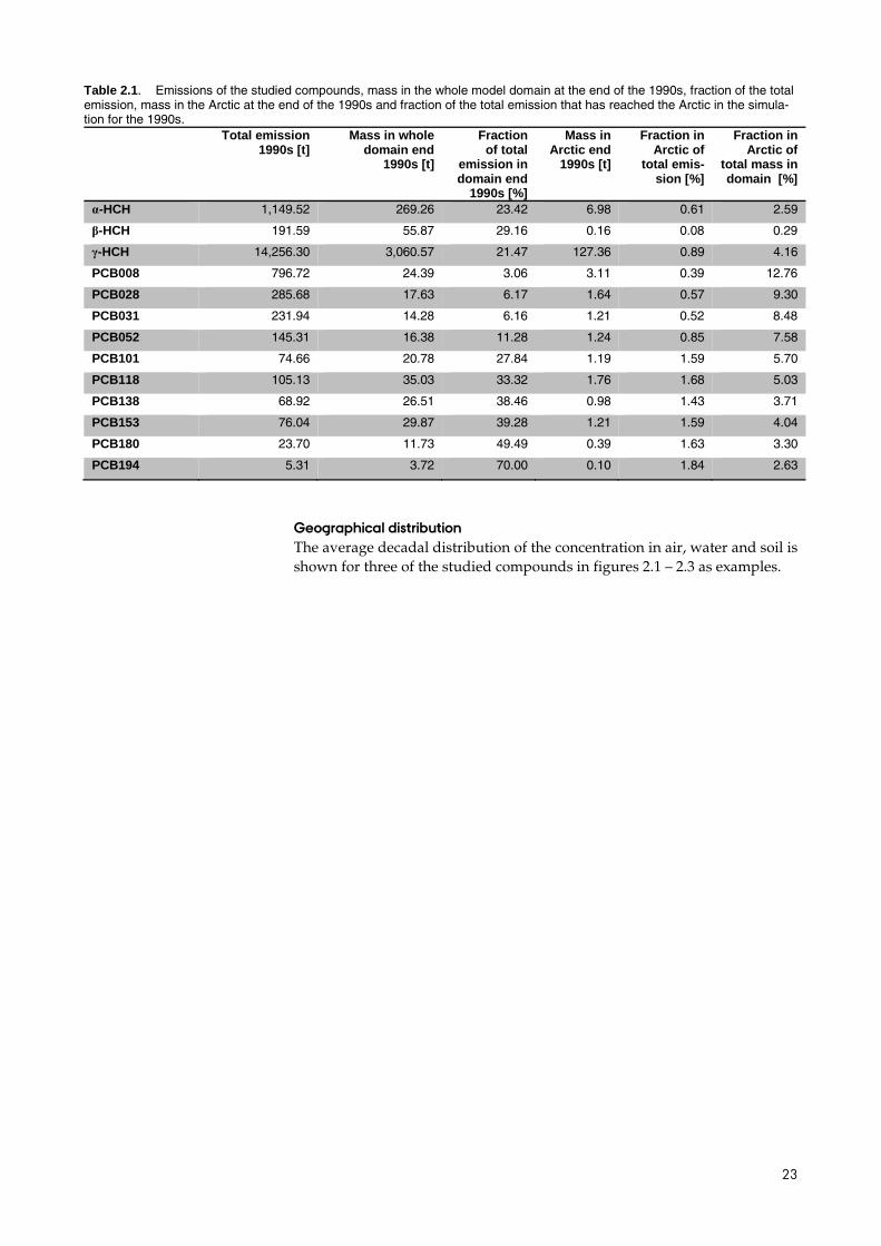
23

Table 2.1. Emissions of the studied compounds, mass in the whole model domain at the end of the 1990s, fraction of the total emission, mass in the Arctic at the end of the 1990s and fraction of the total emission that has reached the Arctic in the simula-tion for the 1990s.

Total emission 1990s [t]

Mass in whole domain end

1990s [t]

Fraction of total

emission in domain end

1990s [%]

Mass in Arctic end

1990s [t]

Fraction in Arctic of

total emis-sion [%]

Fraction in Arctic of

total mass in domain [%]

α-HCH 1,149.52 269.26 23.42 6.98 0.61 2.59

β-HCH 191.59 55.87 29.16 0.16 0.08 0.29

γ-HCH 14,256.30 3,060.57 21.47 127.36 0.89 4.16

PCB008 796.72 24.39 3.06 3.11 0.39 12.76

PCB028 285.68 17.63 6.17 1.64 0.57 9.30

PCB031 231.94 14.28 6.16 1.21 0.52 8.48

PCB052 145.31 16.38 11.28 1.24 0.85 7.58

PCB101 74.66 20.78 27.84 1.19 1.59 5.70

PCB118 105.13 35.03 33.32 1.76 1.68 5.03

PCB138 68.92 26.51 38.46 0.98 1.43 3.71

PCB153 76.04 29.87 39.28 1.21 1.59 4.04

PCB180 23.70 11.73 49.49 0.39 1.63 3.30

PCB194 5.31 3.72 70.00 0.10 1.84 2.63

Geographical distribution The average decadal distribution of the concentration in air, water and soil is shown for three of the studied compounds in figures 2.1 – 2.3 as examples.

24

Figure 2.1. The average decadal distribution of α-HCH concentrations within the model domain for the 1990s (left), the 2090s (middle) and the difference in per cent (right) for air (top), water (middle) and soil (bottom)

25

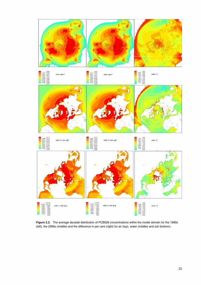
Figure 2.2. The average decadal distribution of PCB028 concentrations within the model domain for the 1990s (left), the 2090s (middle) and the difference in per cent (right) for air (top), water (middle) and soil (bottom).

26

Figure 2.2. The average decadal distribution of PCB180 concentrations within the model domain for the 1990s (left), the 2090s (middle) and the difference in per cent (right) for air (top), water (middle) and soil (bottom).

27

Within the entire model domain around 90% of the three HCHs are found in water in the 1990s (Figure 2.4). The predominant medium for all PCB conge-ners is soil (45% – 90%). For the least chlorinated congeners the fraction found in air is 10% as a maximum for the PCB congeners, while the fraction in air is negligible for the intermediate and most chlorinated congeners. The fraction associated with soil is lowest for the intermediate chlorinated congeners and higher – up to 35% – for the least and most chlorinated congeners.

Only small differences in the inter-media distribution is found between the 1990s and the 2090s (Figure 2.5). The most notable change is in the snow com-partment, with 45 – 70% decrease (Figure 2.6), but since the mass in snow is so small compared to the other media this does not change the inter-media dis-tribution pattern. It is also interesting that the mass in air is increasing for the HCHs and the lowest chlorinated PCB congeners (Figure 2.6).

Figure 2.3. The distribution of the studied compounds between the five media in the entire model domain in the end of the 1990s.

Figure 2.4. The distribution of the studied compounds between the five media in the entire model domain in the end of the 2090s.

0%

10%

20%

30%

40%

50%

60%

70%

80%

90%

100%

Soil

Water

Vegetation

Snow

Air

0%

10%

20%

30%

40%

50%

60%

70%

80%

90%

100%

Soil

Water

Vegetation

Snow

Air

28

Within the Arctic, water is the dominant media for all the studied com-pounds (Figure 2.7). For the HCHs, higher fractions are found in soil than in the entire model domain, the fraction found in snow is considerable alt-hough there is no distinct pattern between the fraction in snow and the chlo-rination of the PCB congeners. A higher fraction is found in air for all com-pounds as well.

Within the Artic, the difference in inter-media distribution between the 1990s and the 2090s is larger than for the whole model domain (Figure 2.8). For the HCHs, larger fractions are found in ocean water for the 2090s, due to higher mass in the water compartment in the simulation for the 2090s (Fi-gure 2.9). For the PCBs the fraction in soil is larger and for the intermediate chlorinated congener it is dominating. This can be explained by an increase in mass in soil for the PCB congeners rather than a decrease in other media. Smaller fractions are found in snow for all compounds, coinciding with de-creases in mass in snow for all studied compounds.

Figure 2.5. Relative changes in total mass in the different media within the model do-main between the 1990s and the 2090s.

Figure 2.6. The distribution of the studied compounds between the five media in the Arctic by the end of the 1990s.

-80

-60

-40

-20

0

20

40

60

Diffe

renc

e[%

]

Air

Snow

Vegetation

Water

Soil

0%

10%

20%

30%

40%

50%

60%

70%

80%

90%

100%

Soil

Water

Vegetation

Snow

Air

29

The contribution from the different regions in the 1990s and the 2090s. The fraction emitted in each of the three source areas is shown in Figure 2.10. Most of the HCHs are emitted from Asia (more than 60%), with only a small fraction of α- and β-HCH emitted in North America. For the PCBs, highest emissions are seen in Europe, while the emission pattern differs from region to region. In North America, the highest emissions are seen for the least and the most chlorinated congeners, whereas in Asia the highest emissions are seen for the intermediate chlorinated congeners. For Europe no distinct pattern is seen.

Figure 2.7. The distribution of the studied compounds between the five media in the Arctic by the end of the 2090s.

Figure 2.8. The changes in mass within the Arctic for the 1990s to the 2090s.

0%

10%

20%

30%

40%

50%

60%

70%

80%

90%

100%

Soil

Water

Vegetation

Snow

Air

-80

-60

-40

-20

0

20

40

60

80

Diffe

renc

e [%

]

Air

Snow

Vegetation

Water

Soil

30

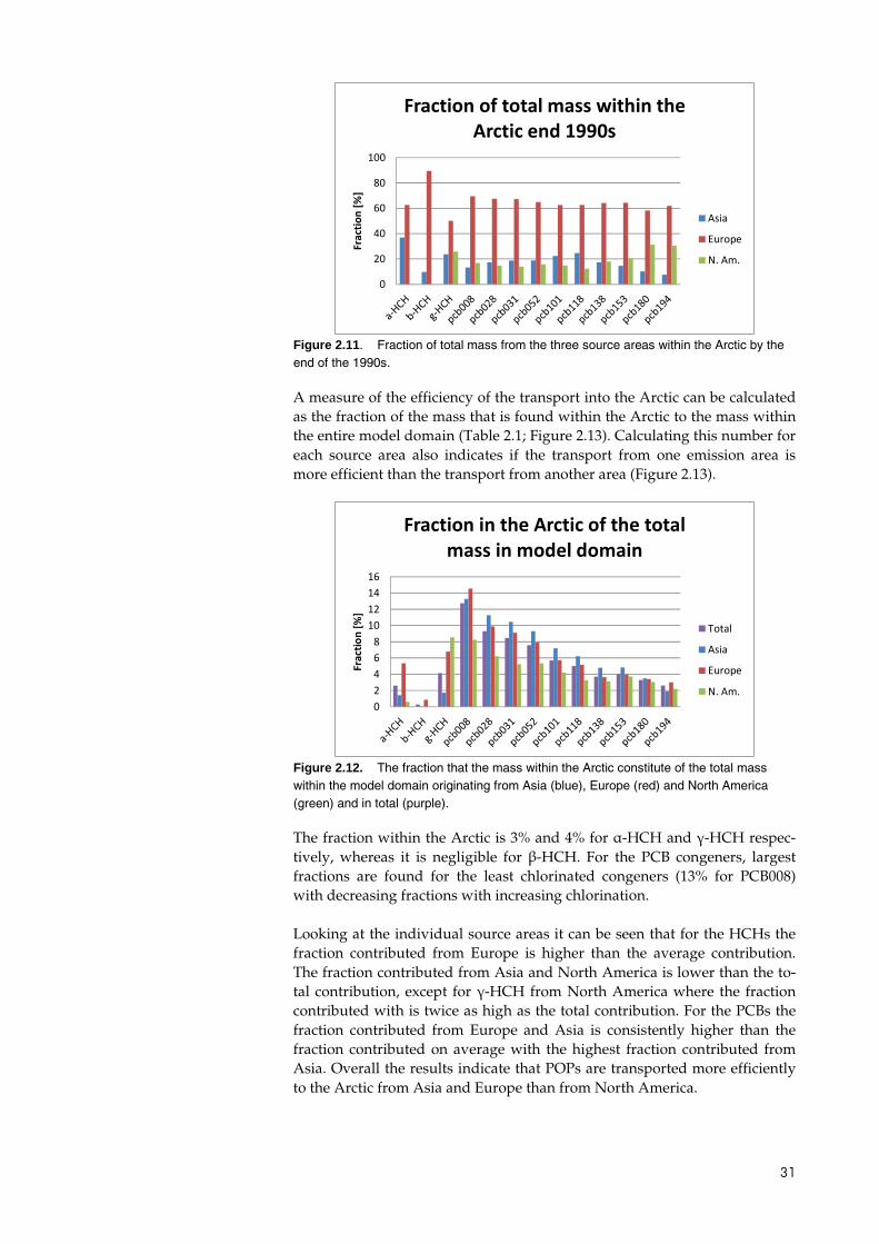
The distribution between the fractions originating from the three regions re-sembles the emission pattern (Figure 2.11). Asia is the major contributor to the total mass within the model domain for the three HCHs. North America only contributes with insignificant amounts of α- and β-HCH, whereas the contribution to γ-HCH is about 13%. Europe is the major contributor to the total mass of the PCB congeners. Small differences in the contribution be-tween the regions with relatively higher contribution of the least and the most chlorinated congeners in North America and relatively higher contri-bution of the intermediate chlorinated congeners from Asia reflect different use patterns in the different regions.

For the Arctic the major contributor for the HCHs is Europe (Figure 2.12). Europe is also the major contributor to the total mass within the Arctic for the PCB congeners but the fraction originating from Asia is slightly higher than for the entire model domain. The fraction from North America tends to be similarly smaller with the fraction from European sources almost similar.

Figure 2.9. The fraction of the total emission emitted in each of the three source areas: North America (NA; green), Europe (EU; red) and Asia (Asia; blue).

Figure 2.10. Fraction of total mass from the three source areas within the entire model domain by the end of the 1990s.

010203040506070

aHCH

b-HC

H

gHCH

PCB0

08

pcb0

28

PCB0

31

pcb0

52

pcb1

01

PCB1

18

PCB1

38

PCB1

53

PCB1

80

PCB1

94

Frac

tion

[%]

Fraction emitted in each of the source areas

Asia

EU

NA

01020304050607080

Frac

tion

[%]

Fraction of total mass within the entire model domain end 1990s

Asia

Europe

N. Am.

31

A measure of the efficiency of the transport into the Arctic can be calculated as the fraction of the mass that is found within the Arctic to the mass within the entire model domain (Table 2.1; Figure 2.13). Calculating this number for each source area also indicates if the transport from one emission area is more efficient than the transport from another area (Figure 2.13).

The fraction within the Arctic is 3% and 4% for α-HCH and γ-HCH respec-tively, whereas it is negligible for β-HCH. For the PCB congeners, largest fractions are found for the least chlorinated congeners (13% for PCB008) with decreasing fractions with increasing chlorination.

Looking at the individual source areas it can be seen that for the HCHs the fraction contributed from Europe is higher than the average contribution. The fraction contributed from Asia and North America is lower than the to-tal contribution, except for γ-HCH from North America where the fraction contributed with is twice as high as the total contribution. For the PCBs the fraction contributed from Europe and Asia is consistently higher than the fraction contributed on average with the highest fraction contributed from Asia. Overall the results indicate that POPs are transported more efficiently to the Arctic from Asia and Europe than from North America.

Figure 2.11. Fraction of total mass from the three source areas within the Arctic by the end of the 1990s.

Figure 2.12. The fraction that the mass within the Arctic constitute of the total mass within the model domain originating from Asia (blue), Europe (red) and North America (green) and in total (purple).

0

20

40

60

80

100

Frac

tion

[%]

Fraction of total mass within the Arctic end 1990s

Asia

Europe

N. Am.

02468

10121416

Frac

tion

[%]

Fraction in the Arctic of the total mass in model domain

Total

Asia

Europe

N. Am.

32

The change in contribution from the different regions from the 1990s to the 2090s A way of examining the influence of climate change on the fate of POPs is by comparing the total mass of the studied compounds within the model do-main from the two simulations (Figure 2.14).

For the total emissions (purple bars in Figure 2.14) we can see that the total mass of α-HCH within the model domain is 6% lower for the 2090s simulation than for the 1990s, β-HCH is 1% higher and γ-HCH is less than one per cent lower. The mass for all the PCB congeners are lower for the 2090s, although with large differences ranging from 21% for PCB008 to 1% for PCB138. Lowest difference is seen for the intermediate chlorinated congeners with larger dif-ferences for both the least and the most chlorinated congeners.

Highest difference between the simulated mass in the 1990s and the 2090s within the Arctic is 43% found for β-HCH (Figure 2.15). This is due to a much higher contribution from North America (129%). However, the contri-bution from North America to the Arctic is very small (≈1kg), thus only a slightly higher contribution in kg for the 2090s will result in a much higher contribution in per cent relative to the 1990s.The mass of both α- and γ-HCH are 21% and 29% higher, respectively. The mass of the three least chlorinated PCB congeners is lower for the 2090s, whereas the mass for the more chlo-

Figure 2.13. The difference in mass between the 1990s and the 2090s in the entire model domain for the total mass (purple), the mass originating from Asia (blue), Europe (red) and North America (green).

Figure 2.14. The difference in mass between the 1990s and the 2090s in the Arctic for the total mass (purple), the mass originating from Asia (blue), Europe (red) and North America (green).

-25.00 -20.00 -15.00 -10.00

-5.00 -

5.00 10.00

Diffe

renc

e [%

]

Difference in mass in whole model domain from 1990s to 2090s

Total

Asia

Europe

N. Am.

-30-20-10

01020304050

Diffe

renc

e [%

]

Difference in mass in the Arctic from 1990s to 2090s

Total

Asia

Europe

N. Am.

129

33

rinated congeners are higher with a tendency of largest difference for the most chlorinated congeners. PCB194 is an exception to the pattern with slightly lower mass in the 2090s (-2%). For all the PCB congeners the contri-bution from Asia appears to decrease in importance compared to the other source areas, i.e. it is lower for most of the congeners, and for the congeners where it is higher in the 2090s, the difference is smaller than the difference for the other source areas.

2.1.2 Hypothetical POPs

The Arctic contamination potential normalised to cumulated emissions (eACP; Wania, 2006) was calculated for a range of hypothetical POPs span-ning the physical-chemical phase space for log Koa values between 3 and 12 and log Kaw values between -4 and 3. eACP is shown in Figure 2.16. Note that similarly to Wania (2003) we have discarded the simulations for com-pounds with log Kow ≥ 10 (upper right corner in Figure 2.16).

Highest potential (12%) for reaching the Arctic surface compartments is seen for compounds with low log Koa and low log Kaw values. These are relative water soluble compounds referred to as “swimmers” (Wania, 2003). A smaller local maximum (of around 4%) is fund for compounds with low log Kaw and high log Koa values. These are compounds that tend to bind to or-ganic fractions in aerosols, soil and vegetation. However, we believe that this may be an artefact in the model which is subject for further research and not discussed further in this report.

For the 2090s, the overall pattern of the eACP phase space is similar to the pattern for the 1990s (Figure 2.16). eACP is generally larger for the 2090s than for the 1990s, with a maximum of 15%. For compounds with log Kaw values larger than -2 and log Koa values smaller than 7 the eACP is smaller for the 2090s than for the 1990s. The difference in per cent between the two decades is shown in Figure 2.17.

Figure 2.15. Arctic contamination potential (eACP) for the 1990s (left) the 2090s (right) calculated using DEHM.

34

Largest differences are for compounds with log Kaw = -4 and log Koa = 8 which is 50% higher for the 2090s than for the 1990s, whereas for log Kaw = 1 and log Koa = 3 the eACP is 68% lower for the 2090s than for the 1990s. It should be noted that the eACP is very close to zero for the latter case, whereas it is only a few per cent for the former.

We have also calculated the eACP for compounds emitted in Europe, Asia and North America respectively, see figures 2.18-2.23. Here the mass in the surface compartments in the Arctic arising from emissions in each of the source areas is normalised with the emissions from that source area.

Figure 2.16. The difference between the eACP for the 1990s and the 2090s.

Figure 2.17. Arctic contamination potential (eACP) for compounds emitted in Europe for the 1990s (left) the 2090s (right) calculated using DEHM.

35

Figure 2.18. The difference between the eACP for the 1990s and the 2090s for com-

pounds emitted in Europe.

Figure 2.19. Arctic contamination potential (eACP) for compounds emitted in Asia for the 1990s (left) the 2090s (right) calculated using DEHM.

36

Figure 2.20. The difference between the eACP for the 1990s and the 2090s for com-pounds emitted in Asia.

Figure 2.21. Arctic contamination potential (eACP) for compounds emitted in North America for the 1990s (left) the 2090s (right) calculated using DEHM.

37

The eACP for the individual emission areas have similar pattern as the over-all eACP, with maximum for low log Kaw and low log Koa values. Highest eACP is found for emissions from Asia (42%), with 25% for North America and 17% for Europe as the highest eACP for the 1990s. For the 2090s, the maxima are 58% for Asia, 35% for North America and 23% for Europe.

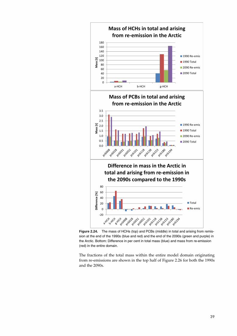
2.2 Contribution from reemissions We have made two simulations where the fraction of the compounds that we kept track on using the tagging method was the part re-emitted to the atmosphere after being deposited. In this way we can estimate how much of a compound that originates from primary emissions and how much has been transported via multi-hop transport. In Figure 2.24 the total mass with-in the domain by the end of the 1990s and the 2090s and the total mass origi-nating from re-emissions within the domain by the end of the 1990s and the 2090s is plotted. The total mass by the end of the 1990s and the 2090s is 6% lower for α-HCH, whereas there are only small differences for the other two HCH isomers. The mass originating from re-emission is higher: 0.5%, 11% and 7% for α-, β-, and γ-HCH. The total mass of the PCBs is between 1% and 21% lower in the 2090s than in the 1990s, and for the re-emitted part it is up to 30% lower, except for PCB101, where the re-emitted part is 3% higher. For the lowest chlorinated congeners (up to PCB101) the changes in total mass are higher than the changes in the re-emitted mass, and for the higher chlo-rinated congeners the changes in the re-emitted mass are higher.

Figure 2.22. The difference between the eACP for the 1990s and the 2090s for com-pounds emitted in North America.

38

In Figure 2.25, the same data are shown for the mass within the Arctic. Here it can be seen that the mass of the HCHs is higher in the 2090s than in the 1990s both in total and for the part arising from re-emissions. For the PCBs, the total mass is lower for the three least chlorinated congeners and for the most chlorinated congener, whereas it is higher for the rest. The mass arising from re-emission is higher in the 2090s for all congeners except the PCB008 and PCB194. The change in mass from re-emission is lower than the change in total mass for the intermediate congeners, whereas it is higher for the least chlorinated congeners and for PCB194.

Figure 2.23. The mass of HCHs (top) and PCBs (middle) in total and arising from remis-sion at the end of the 1990s (blue and red) and the end of the 2090s (green and purple) in the entire domain. Bottom: Difference in per cent in total mass (blue) and mass from re-emission (red) in the entire domain.

0

500

1,000

1,500

2,000

2,500

3,000

3,500

a-HCH b-HCH g-HCH

Mas

s [t]

Mass of HCHs in total and arising from re-emission in domain

1990 Re-emis

1990 Total

2090 Re-emis

2090 Total

05

10152025303540

Mas

s [t]

Mass of PCBs in total and arising from re-emission in domain

1990 Re-emis

1990 Total

2090 Re-emis

2090 Total

-40-30-20-10

01020

Frac

tion

[%]

Difference in mass in the Arctic in total and arising from re-emission in

the 2090s compared to the 1990s

Total

Re-emis

39

The fractions of the total mass within the entire model domain originating from re-emissions are shown in the top half of Figure 2.26 for both the 1990s and the 2090s.

Figure 2.24. The mass of HCHs (top) and PCBs (middle) in total and arising from remis-sion at the end of the 1990s (blue and red) and the end of the 2090s (green and purple) in the Arctic. Bottom: Difference in per cent in total mass (blue) and mass from re-emission (red) in the entire domain.

020406080

100120140160180

a-HCH b-HCH g-HCH

Mas

s [t]

Mass of HCHs in total and arising from re-emission in the Arctic

1990 Re-emis

1990 Total

2090 Re-emis

2090 Total

0.0

0.5

1.0

1.5

2.0

2.5

3.0

3.5

Mas

s [t]

Mass of PCBs in total and arising from re-emission in the Arctic

1990 Re-emis

1990 Total

2090 Re-emis

2090 Total

-20

0

20

40

60

80

Diffe

renc

e [%

]

Difference in mass in the Arctic in total and arising from re-emission in

the 2090s compared to the 1990s

Total

Re-emis

40

For the 1990s, highest HCH fractions are seen for α-HCH with 37% and for γ-HCH (29%). For the PCBs the fraction is between 16% and 32%, with low-est fractions for the intermediate chlorinated congeners and highest for the least chlorinated (PCB008; 21%) and the most chlorinated (PCB153 and above; 18% – 32%). The fraction of re-emitted compounds within the entire model domain is higher in the 2090s than in the 1990s for the HCHs and for the least chlorinated PCB congeners (PCB101 and lower) whereas it is lower for the higher chlorinated PCB congeners with largest difference for PCB194.

The fractions of the mass in all media within the Arctic originating from re-emissions are shown in Figure 2.27 for both the 1990s and the 2090s.

The fractions of the mass in all media within the Arctic originating from re-emissions are higher for all compounds than for the entire model domain. Highest fractions are found for the most chlorinated PCB congeners, with 77% for PCB194. The fraction is gradually lower for the less chlorinated con-geners with lowest fraction for PCB008 (30%). Highest fraction for the HCHs is found for α-HCH (46%) and lowest for β-HCH (27%). The fraction of re-emitted compounds is also higher within the Arctic in the 2090s than in the 1990s for the HCHs and for the least chlorinated PCB congeners (PCB052 and lower) whereas it is lower for the higher chlorinated PCB congeners.

Figure 2.25. Fraction of mass in all media within the model domain originating from re-emissions in the end of the 1990s (blue) and 2090s (red).

Figure 2.26. Fraction of mass in all media within the Arctic originating from re-emissions in the end of the 1990s (blue) and 2090s (red).

0

10

20

30

40

50

Fraction of total mass within the whole model domain originating

from re-emissions end '90s

1990s

2090s

0

20

40

60

80

100

Fraction of total mass within the Arctic originating from re-emissions

end '90s

1990s

2090s

41

2.3 Contribution from climate change versus emission change

Four model simulations were performed to illustrate how the future climate changes versus the future emission changes affect the fate of POPs. The monthly averaged mass within the domain for the four simulations is shown in Figure 2.28.

Figure 2.27. Monthly average total mass within the model domain of PCB028 (top), PCB153 (middle) and PCB180 (bottom) with climate and emissions for the 1990s (C19E19, blue), with climate for the 2090s and emissions from the 1990s (C20E19, red), with climate for the 1990s and emission for the 2090s (C19E20, green) and with climate and emissions for the 2090s (C20E20, purple).

05

1015202530354045

feb-

90ok

t-90

jun-

91fe

b-92

okt-

92ju

n-93

feb-

94ok

t-94

jun-

95fe

b-96

okt-

96ju

n-97

feb-

98ok

t-98

jun-

99

Mas

s [t]

Mas of PCB028 within in the domain

C19E19

C20E19

C19E20

C20E20

500550600650700750800850900950

1,000

feb-

90ok

t-90

jun-

91fe

b-92

okt-

92ju

n-93

feb-

94ok

t-94

jun-

95fe

b-96

okt-

96ju

n-97

feb-

98ok

t-98

jun-

99

Mas

s [t]

PCB153 within the domain

C19E19

C20E19

C19E20

C20E20

800

850

900

950

1,000

1,050

1,100

1,150

1,200

feb-

90ok

t-90

jun-

91fe

b-92

okt-

92ju

n-93

feb-

94ok

t-94

jun-

95fe

b-96

okt-

96ju

n-97

feb-

98ok

t-98

jun-

99

Mas

s [t]

PCB180 within the domain

C19E19

C20E19

C19E20

C20E20

42

The large difference in applied emissions for the 1990s and the 2090s results in clear differences in the simulated masses between the simulations with emissions for the 1990s (E19) and the simulations with emissions for the 2090s (E20). For PCB028 the total mass decreases through the modelled de-cade for all four simulations. There is a large decrease in the simulated mass during the first year especially for the E20 simulations. The reason for this is that the input data for the simulations are from another model with different properties of the surface compartments. The data are thus in another state of equilibrium between the media and the inter-media distribution is adjusted in DEHM with large fluxes during the first year before the inter-media dis-tribution reaches a new overall equilibrium in DEHM. This also applies for the other simulated compounds. A clear seasonal signal is seen for the E19 simulations with highest mass in April, whereas there is no seasonal pattern for the E20 simulations. The mass decreases more rapidly for the C20 simu-lations than for the C19 simulations. The mass of PCB153 increases through the modelled decades for the E19 simulations, whereas it decreases for the E20 simulations. The increase for the C20E19 is less rapid than for the C19E19, and the decrease for the C20E20 is more rapid than for the C19E20 simulation. Seasonal signals are seen for the E19 simulations of PCB153 with highest mass found in the summer months, whereas there is no seasonal signal for the E20 simulations. The mass of PCB180 follow the same pattern as PCB153. The increase for the E19 simulations is more rapid than for PCB153.

The monthly averaged mass within the Arctic is seen in Figure 2.29.

The mass of all the studied PCB congeners within the Arctic decrease in all four simulations. The most remarkable difference is that the mass of PCB180 is higher in the E20 emission scenarios than in the E19 emission scenarios.

To quantify the effect of climate and emission changes we have calculated the difference in per cent between the average mass in the final year of the simulations (Figure 2.30). It is evident that the change in emission is causing the largest difference. This is expected given the large difference between the emissions for the two decades (table 1.1) however the effect is highly differ-ent for the three congeners. For PCB028 the effect of changed climate for the 1990s is a difference in predicted mass of 27%, whereas for the 2090s emis-sion scenario with much lower emissions, the effect is a difference of 65%.The combined effect of climate and emission change is not much larger than the effect of emission change for PCB028. For the more chlorinated PCB congeners the effect of the climate change is about a 1% difference in pre-dicted mass. The effect of changed emissions is 41% and 24% difference in predicted mass for PCB153 and PCB180, respectively. The combined effect of climate and emission change is only slightly larger than the effect of emis-sion change alone.

43

Figure 2.28. Monthly average total mass within the Arctic of PCB028 (top), PCB153 (middle) and PCB180 (bottom) with climate and emissions for the 1990s (C19E19, blue), with climate for the 2090s and emissions from the 1990s (C20E19, red), with climate for the 1990s and emission for the 2090s (C19E20, green) and with climate and emissions for the 2090s (C20E20, purple).

0

2

4

6

8

10

12

14

feb-

90ok

t-90

jun-

91fe

b-92

okt-

92ju

n-93

feb-

94ok

t-94

jun-

95fe

b-96

okt-

96ju

n-97

feb-

98ok

t-98

jun-

99

Mas

s [t]

PCB028 within the Arctic

C19E19

C20E19

C19E20

C20E20

100

110

120

130

140

150

160fe

b-90

okt-

90ju

n-91

feb-

92ok

t-92

jun-

93fe

b-94

okt-

94ju

n-95

feb-

96ok

t-96

jun-

97fe

b-98

okt-

98ju

n-99

Mas

s [t]

PCB153 within the Arctic

C19E19

C20E19

C19E20

C20E20

120

125

130

135

140

145

feb-

90ok

t-90

jun-

91fe

b-92

okt-

92ju

n-93

feb-

94ok

t-94

jun-

95fe

b-96

okt-

96ju

n-97

feb-

98ok

t-98

jun-

99

Mas

s [t]

PCB180 within the Arctic

C19E19

C20E19

C19E20

C20E20

44

Within the Arctic the effects are smaller than in the entire model domain. For PCB028, the magnitude of the effects is almost the same (Figure 2.31). For PCB 153, the effect of a changed climate is a difference in predicted mass of 4% and 5% for the two emission scenarios. The effect of changed emissions is only a difference of 10% although the emissions are several orders of magnitude lower. The combined effect of climate and emission change is a difference of 14%. For PCB180 the effect of a changed climate is around 2% for the two emission scenarios. However, the predicted masses in the Arctic for the simu-lations using the 2090s emission scenario are higher than the predicted masses for the simulations using the 1990s emission scenario. The effect of changed

Figure 2.29. The effect of climate change under the two emission scenarios (E19 and E20), the effect of emission change and the combined effect of climate and emission change on the mass of PCB028 (top), PCB153 (middle) and PCB180 (bottom) within the model domain. All numbers are in per cent.

Effect climate E19 26.61Effect climate E20 64.86Effect emission 97.21Effect climate + emission 97.95

0

20

40

60

80

100

Diffe

renc

e [%

]

Effect on mass of PCB028 at the end of the '90s within the domain

Effect climate E19 1.40Effect climate E20 1.70Effect emission 40.85Effect climate + emission 41.68

05

1015202530354045

Diffe

renc

e [%

]Effect on mass of PCB153 at the end

of the '90s within the domain

Effect climate E19 1.18Effect climate E20 0.76Effect emission 24.24Effect climate + emission 25.13

05

1015202530

Diffe

renc

e [%

]

Effect on mass of PCB180 at the end of the '90s within the domain

45

emissions is therefore predicted to be an increase in mass within the Arctic of 5%, whereas the combined effect of climate and emission change is a 3% dif-ference in predicted mass.

Figure 2.30. The effect of climate change under the two emission scenarios (E19 and E20), the effect of emission change and the combined effect of climate and emission change on the mass of PCB028 (top), PCB153 (middle) and PCB180 (bottom) within the Arctic. All numbers are in per cent.

Effect climate E19 30.20Effect climate E20 64.29Effect emission 87.90Effect climate + emission 91.55

0

20

40

60

80

100

Diffe

renc

e [%

]

Effect on mass of PCB028 at the end of the '90s within the Arctic

Effect climate E19 4.07Effect climate E20 5.24Effect emission 10.48Effect climate + emission 14.13

02468

10121416

Diffe

renc

e [%

]

Effect on mass of PCB153 at the end of the '90s within the Arctic

Effect climate E19 1.78Effect climate E20 2.10Effect emission -5.20Effect climate + emission -3.32

-6-5-4-3-2-10123

Diffe

renc

e [%

]

Effect on mass of PCB180 at the end of the '90s within the Arctic

46

3 Results for Hg

In this section we have used the results primarily obtained from the mercury sub-model of DEHM (Christensen et al. 2004). The applied mercury chemi-stry scheme is based on GKSS chemistry (Petersen et al., 1998), which con-sists of 3 gas phase compounds: Hg0, HgO, HgCl2, 1 particulate phase Hg and 9 aqueous phase compounds. In this scheme ozone is the most im-portant oxidant for the formation of RGM and TPM. During polar sunrise over sea-ice in the Arctic an additional fast oxidation rate of Hg0 to HgO is assumed in order to simulate the Atmospheric Mercury Depletion Events (AMDE). It is a simple, but useful, parameterization. In the model simula-tions, presented here, there are no re-emissions after AMDE in the Arctic, which means that the calculated total deposition of Hg is a high model esti-mate of the Hg deposition in the Arctic. Furthermore, the model does not have Mercury emissions from ocean and soil, which are also important sources of atmospheric Hg0. The contributions from these sources are as-sumed to be included in the global background concentration of Hg0 of 1.5 ng/m3, which is used as initial and boundary conditions in all the simula-tions. This background concentration represents the current background concentration depending on the current anthropogenic and natural emis-sions as well as re-emissions. However, it is possible to estimate the influ-ence of the anthropogenic emissions on the background concentration via post processing if the contribution from the global background concentra-tion is known. This is done by assuming that only emissions of Hg0 contrib-ute to the global background concentration and that the natural emissions and re-emissions are assumed to be unchanged with 4200 tons Hg (the value of natural and re-emissions are obtained from AMAP 2011):

Hg0back=1.5ng/m3·(Hg0used_emis + 4200tons)/( Hg0emis2005 + 4200tons).

In all the simulations presented here the contribution form the background concentration is known. Therefore this post processing procedure has been used for all the presented results.

The ozone concentrations are provided by the SOx-NHx-NOx-O3-VOC chem-istry module. Furthermore, Black Carbon concentrations, which are applied in the model for the production of particular Hg in the aqueous phase chem-istry, are provided by the particle module in DEHM.

DEHM performs well with input of real meteorology from e.g. the MM5 weather forecast model (Brandt et al., 2012), which is using global analyzed meteorological data as input. By using climate meteorological data from ECHAM5/MPI-OM (SRES A1B scenario) as in this project for two different decades: 1990-1999 and 2090-2099 instead of MM5 based data, it is possible to investigate the response of DEHM to a changed climate e.g. on the atmos-pheric deposition of Hg in the Arctic. This is a sensitivity analysis to investi-gate the response of the model system to changed climate input. One thing that should be kept in mind with the interpretation of such sensitivity ana-lyses is that the model, as many other models, has parameterizations of pro-cesses, which are tuned to the current climate in order to improve the model performance. The processes may change with climate conditions and the model may thus not have a reliable response to a changed climate input.

47

3.1 Contribution from major source areas (Europe, Asia, North America and Global Background)

With the present parameterization of the Hg module in DEHM there are no non-linear processes. We have therefore chosen not to apply the tagging method to study the influence of different source areas but used the subtrac-tion method described above, which is less computational demanding. For each of the two climate decades 4 different model simulations were per-formed:

1. All sources 2. No sources in North America (NA) 3. No sources in Europe (EU) 4. No sources in Asia (AS)

By using these model simulations it is possible to estimate the contribution from the different source areas including the boundary and initial conditions of Hg0, i.e. the contribution form the global background concentration. In Figure 3.1 the mean concentrations of Hg0, Reactive Gaseous Mercury (RGM=HgO+HgCl2) and Total Particular Mercury (TPM=primary + oxi-dized particulate Hg) and the contribution from the different source areas are shown. The mean concentration of Hg0 is 3.8% higher in 2090-2099 com-pared to 1990-1999, while the concentrations of both RGM and TPM are 41% and 62% lower. The main reason for these changes in the model is that dur-ing the Arctic mercury depletion events Hg0 is oxidized very fast to HgO and the parameterization of this oxidation depends on the sea-ice fraction. The decreasing sea-ice fraction in 2090-2099 compared to 1990-1999 will re-sult in a decreased oxidation of Hg0 to HgO. For both Hg0 and RGM the global background contributes with up to 64% of the total concentration, while Asia contributes with about 25%, about 6% comes from Europe and finally 5% arrives from North America. For particular Hg the contribution form the background is smaller (about 45%), mainly because of the transport of primary particular Hg, especially from Europe. There are no large chan-ges in the contributions for the two decades, which means that relative con-tribution from the different sources does not depend on the climate accor-ding to the model simulations.

48

In Figure 3.2 the total annual deposition of Hg north of Polar Circle is shown. There is a significant decrease of about 18% of the total deposition from 1990-1999 to 2090-2099. The reason is the same as mentioned above for the decrease of RGM concentrations, that during AMDE Hg0 is oxidized to RGM, which has a high dry deposition to the surface, and this oxidation de-pends on the sea-ice fraction. With a decreasing sea-ice fraction the concen-trations of RGM will decrease and therefore the dry deposition will de-crease. In Figure 3.2 the relative contribution is also shown and these are quite similar to the relative contributions of Hg0 concentrations as described above, reflecting that Hg is transported to Arctic as Hg0 and Hg0 is oxidized to RGM (and particular Hg) during the transport and some of this oxidized Hg is deposited. The global background is the most important source. There are only very small differences in the relative contributions for the two dec-ades indicating that climate change do not have a large influence on the rela-tive contribution of the source areas. All the source areas in the Northern Hemisphere contributes to a large background pool of Hg0 and this is get-ting well mixed before the Hg are deposit because of the long lifetime of Hg0 in the atmosphere (1 year).

Figure 3.1. The Artic average concentrations of Hg0 (upper), RGM (lower left) and TPM (lower right) for the two studied dec-ades divided into the contribution from Europe (EU), Asia (AS), North America (NA) and the background.

49

However, there are some differences between the source areas in how large a fraction of the total emission that is deposited in the Arctic (Figure 3.3). Eu-rope is relatively the most important source area from which around 4.5% of the total Hg emission is deposited in the Arctic, while it is around 3.4% for Asia and 3.2% for North America for the 1990-1999 decade. This indicates that the emissions placed in Europe are more efficiently transported to the Arctic compared to emission from Asia and especially North America, which both are located more southerly and also have a longer transport path/time over ocean before they arrive in the Arctic. Common for all 3 source areas is that this fraction is lower in the 2090-2099 compared to 1990-1999 because of the lower deposition due to the decreased sea-ice fraction.

3.2 The contribution from 2020 emission changes vs. climate changes

In the basic simulation we used the global Mercury emission inventory for 2005 (Pacyna et al, 2010). This was also used above for the climate simula-tions with source contribution estimates. To study the effect of emission changes versus the effect of climate changes, three different emission scenar-ios were used for the target year of 2020: the ‘Status Quo’ (SQ) scenario, the ‘Extended Emissions Control’ (EXEC) scenario, and the ‘Maximum Feasible Technological Reduction’ (MFTR) scenario (Pacyna et al., 2010). In figure 3.4 the emissions of Hg0, reactive Hg (rHg), and particular Hg (pHg) are shown. The total emissions inside the model domain for the SQ scenario is 21% higher than the 2005 emissions, while the EXEC and MFTR are 45% and 55% lower.

Figure 3.2. The total deposition of Hg in tons/year with the contribution from the different source areas including indirect con-tribution (left) and the relative contribution from the different source areas to the total deposition of Hg for the Arctic for the two studied decades.

Figure 3.3. The amount of total emitted Hg for the different source areas deposited in the Arctic for the two decades.

50

We have performed 2 basic simulations and 6 different model simulations with the future emission scenarios. The 2 basic simulations are for the 1990-1999 and 2090-2099 decades, both with 2005 emissions and the 6 scenario simulations are also for the two decades, one with each of the three emis-sions scenarios for 2020 as described above. Furthermore, two model simula-tions for the two decades with no anthropogenic emissions, called “zero emission” have also been made. In Figure 3.5 the total deposition in the Arc-tic (left) and the relative changes compared to the 2005 basic simulation for the 1990-1999 decade (right) are shown for all 10 model simulations. The MFTR results in 20% decrease, the EXEC in 16% decrease, while the SQ sce-nario results in a 6% increase of the total deposition compared to the 2005 basic emissions simulation. If all the anthropogenic emissions were set to 0 the deposition to the Arctic will decrease by 37%.

In Figure 3.6 the relative changes of the total mercury deposition to the Arc-tic for all 5 emissions scenarios between the decades 1990-1999 and 2090-2099 is shown. The changes in total deposition for the period 1990-1999 to the period 2090-2099 is around 18% for all 5 emission scenarios. The climate signal is more or less independent of the applied emission scenario.

According to the model simulations presented here the decrease of the Hg deposition due climate changes are smaller than the decrease due to emis-sion changes in the MFTR and “zero emission” scenarios; 18% vs. 20% or 37%. If MFTR and “zero emission” were combined with the predicted depo-sition changes due to changed climate input, then the model system predicts total decreases of the Arctic Hg deposition of 33% for MFTR and 47% for “zero emission” for the end of 21th century compared to end of 20th century.

Figure 3.4. The total yearly emission in tons Hg inside the model domain for the 4 dif-ferent emission scenarios, split up in emission of Hg0, reactive Hg (rHg) and particular Hg (pHg).

Figure 3.5. Total mercury deposition in Tons Hg/year to the Arctic for all different emissions scenarios from DEHM (left) and the relative difference in % (right) for the decades 1990-1999 (blue) and 2090-2099 (red).

51

But as mentioned above these changes in the deposition of Hg predicted by the model due to changes in climate input is a sensitivity study of the model system and does not necessarily reflect a correct climate response in the real atmosphere.

Over time the change of Hg deposition in Arctic due to emission change should be even larger, because the amount of global biologically available Hg in soil and ocean will change slowly due to the changed atmospheric fluxes and the removal of biologically available Hg, e.g. by transport of Hg to the deep ocean or by sedimentation, and this will change the remissions and the global atmospheric background further.

Figure 3.6. The relative changes of the total mercury deposition to the Arctic areas north of Polar Circle for all emissions scenarios between the decades 1990-1999 and 2090-2099.

52

4 Discussion

4.1 Contribution from major source areas (Europe, Asia and North America)

4.1.1 Real POPs

Distribution between the media Relatively larger changes in the distribution between the media were seen for the Arctic than for the entire model domain from 1990s to the 2090s (fig-ures 2.6 and 2.9). This is probably because the climatic changes in the Arctic are larger than the globally averaged changes. The largest relative change for all compounds is for snow, which is expected since the snow cover will re-treat and the snowpack season will be shortened in a future warmer climate. There is thus less snow for the POPs to be associated with. For the HCHs relatively larger fractions were found in the sea. This is because the sea ice cover will retreat. This leads to more open water and thus a larger area where the relatively water soluble HCHs can be deposited to. This is also helped by the increase in wet deposition. The PCB congeners have generally higher Koa values than the HCHs and are thus more associated with organic fractions in e.g. soil and in particles in the air. With a smaller snow cover more will be deposited to the soil, which is the reason for the higher frac-tions of PCBs found in soil within the Arctic. Particles also have a larger deposition velocity to bare soil, which will also increase the transfer of the most chlorinate PCB congeners to soil.

Importance of source areas When comparing the fractions of emissions from each source area (Figure 2.10) with the mass in the Arctic from each source area (Figure 2.12) it can be seen that the contribution to the Arctic from North America generally is smaller than the contribution to the total emissions. One exception is for γ-HCH, where the transport from North America is more efficient than from the other source areas (Figure 2.13). The reason for this is the position of the emissions of γ-HCH in Canada, relatively close to the Arctic. For the HCHs Europe is the most efficient source region in delivering to the Arctic. One possible explanation for this is that the transport to the Arctic from Europe is over land areas, whereas the transport from North America and Asia is largely over oceans (the North Atlantic and the Pacific Oceans, respectively). The HCHs, being relatively water soluble, then gets depleted over the oceans and thus the transport from Europe will appear more efficient. An-other factor that cannot be ruled out is the position of the sources within the region but this requires further studies in order to determine the importance of this factor. The transport of PCBs from Europe is also slightly more effi-cient than on average, however, the transport from Asia is even more effi-cient. Again this can be due to the position of the sources within the region. The transport of the least chlorinated PCB congeners is more efficient than for the higher chlorinated congeners (Figure 2.13), which follows the ideas of the global distillation hypothesis (Wania and Mackay, 1996).

The atmospheric transport from Europe is generally expected to be higher than the transport from other source regions due to the position of the polar front in winter time (AMAP, 1998), but apart from the HCHs there do not appear to be very large differences between the efficiency to transport POPs to the Arctic from Europe and Asia.

53

Looking at the overall change in mass within the model domain, it can be seen that the mass of all PCB congeners is lower for the 2090s than for the 1990s (Figure 2.14). This is due to a shift from surface compartments to the air owing to an increased average temperature. On the same time the degra-dation rates in all media and especially in air increases as the temperature increases. The shift to air enhances the atmospheric transport to the Arctic, which is somewhat counteracted by the increased atmospheric degradation. This leads to larger amounts of some of the PCBs within the Arctic, where the degradation dominates for the least chlorinated congeners (Figure 19). The more chlorinated congeners are more associated with particles due to their higher log Koa values and since no degradation on particle bound com-pounds is assumed in model the effect from the increased atmospheric deg-radation cannot be seen. PCB 194 is an exception to this pattern, which needs to be studied further to be explained.

The mass of the HCHs is higher within the Arctic in the 2090s than in the 1990s. The higher temperature leads to a shift to air for the HCHs as well and the water solubility in combination with an increase in wet deposition and a larger ice free Arctic Ocean leads to enhanced deposition to the Arctic ocean, where the degradation life time is very long (Harner et al., 1999).

The changes in β-HCH are exceptional. However in general the transport of β-HCH to the Arctic is very low in these model simulations and the relative changes are thus not significant. This is partly due to the very low emission, but partly due to its physical-chemical properties since it is more water sol-uble than the other HCH isomers. This leads to a larger depletion before it reaches the Arctic. ß-HCH will eventually reach the Arctic via oceanic transport as described by Li et al. (2002), however, the time scale of this transport is too long to be resolved by the model simulations made in this study.

4.1.2 Hypothetical POPs

The emission normalised Arctic Contamination Potential (eACP) for the 1990s produced in this study (Figure 2.16) has highest values for the most water soluble compounds with low log Koa (=3) and low log Kaw (=-4) val-ues. The ACP concept was developed by Wania (2003; 2006) for which he used the multi-compartment mass balance model Globo-POP, where the world is divided into 10 zonally averaged climatic zones (Wania, 2003). When comparing the overall results it can be seen that the eACP predicted by the two models are within a factor of 2 – 3, although there are notable dif-ferences. With a maximum value of 12% eACP predicted by DEHM exceeds the maximum values of 4.5% calculated by Wania (2006). The overall pre-dicted pattern of the eACP is also slightly different in this study than the Wania study who predicts a maximum eACP for compounds with log Koa =3 and log Kaw =-2 (Wania, 2006). The eACP values predicted by DEHM for this area are 6 – 7%. Furthermore the pattern predicted by Wania (2006) with rel-atively high eACP values of 2 – 2.5% for log Koa =8 and high log Kaw is only discernible in Figure 2.16 with values of around 1%.

The difference in the predicted results between the two models is most probably found in the parameterization of the environmental processes in the two models. The Globo-POP model applies long-term average environ-mental conditions (temperature, wind speeds, precipitation rates, etc.) to de-scribe the environmental processes, where the dynamic meteorological data from the applied input, in this study from the ECHAM climate global circu-

54

lation model with a temporal resolution of 6 hours, is used in DEHM. The most important difference in this context is the parameterization of precipi-tation, which in Globo-POP is described using constant rain rates, whereas precipitation in DEHM has the intermittent nature of the meteorological in-put. The use of constant rain rates in multimedia mass balance models has been shown to affect the atmospheric transport for low log Kaw values (Hertwich, 2001). For relative water soluble compounds the use of constant precipitation rates will lead to relative short transport distances due to rapid deposition, whereas for intermittent precipitation events, long transport can occur during dry spells. Wania is aware of this fact and states that the appli-cation of the constant precipitation rates in Globo-POP is inappropriate for water soluble compounds (Wania, 2003). We therefore hypothesize that the globo-POP underestimate the eACP for the compounds with low log Kaw values, which is the main reason for the discrepancy between the eACP pre-dicted by DEHM and Globo-POP. It should also be noted that the Arctic is not defined in the exact same way in the two models, which may lead to some discrepancies.

Climate change acts to increase the eACP for the most water soluble com-pounds with low log Kaw values (Figure 2.17). It is very interesting to note that α- and γ-HCH with log Kaw values of -3.5 – -4 and log Kao values of 7.5 – 8 is in the area with up to 50% increase in eACP in the 2090s. This coincides with the predicted increase in mass of 20 – 30% in the Arctic by the simula-tions made in the first part of this study (Figure 2.15). The hypothetical chemicals studied in this part are assumed to be perfectly persistent the pre-dicted eACP values may thus be higher than for actual chemical com-pounds. The physical chemical properties of the PCB congeners (low log Kaw and high log Kao values) place them in the areas with relatively low eACP values and in the area with low influence on the eACP by climate change.

The lower eACP predicted by DEHM for compounds with the combination of low log Kao values and high log Kaw values (upper left corner of Figure 2.17) for future climate is probably because the higher temperature in the 2090s acts to shift the compounds from the surface compartments towards air. More of the compounds may then be transported to the Arctic but less will be deposited to the surface compartments where they can enter the food web.

The study of the most important source area contributing to the transport to the Arctic showed that Asia had the highest eACP and Europe had the low-est. One possible explanation for this is that the emissions in Asia are occur-ring under higher temperatures than emissions from the other source areas, which favour transport over deposition relatively close to the source. The re-sults cannot be compared directly but they deviate from the result of the first part of the study in which the least important region contributing to the con-tamination of the Arctic for the PCBs was North America and the differences between the regions were not as large as for this part of the study. We need to study this further before we can make any firm conclusions on this mat-ter.

4.2 Contribution from reemissions The fraction in the Arctic from re-emission is between 27% and 77% in the end of the 1990s. It should be kept in mind that the simulations were made without any initial concentrations in the environment and the results would look different if this was taken into account or if the simulations were made

55

for a longer period. The higher fractions of re-emission within the Arctic than in the entire model domain is an expected result since the sources are relatively far from the Arctic and more of the emitted compounds that reaches the Arctic will have been deposited and re-emitted along the transport route. For the PCBs, the highest fraction of re-emission is seen for the most chlorinated PCB congeners, which is due to the shorter long-range transport potential of the higher chlorinated congeners (Beyer et al., 2000).

The changed climate only result in minor differences in the importance of re-emitted compounds in the Arctic, for the HCHs and the least chlorinated PCB congeners, the fraction is higher and for the most chlorinated PCB con-geners the fraction is lower in the 2090s than in the 1990s (Figure 2.27). This shift in importance of the re-emission between the two simulated decades for the most chlorinated congeners may be counter-intuitive. Higher tem-peratures in the 2090s favour re-emission from the surfaces and we would expect that the fraction from re-emission residing in the Arctic would be higher for all compounds. One possible explanation is that the higher tem-perature will increase the transport potential and thus the transport distance for the compounds emitted in the primary emissions. A larger fraction of the primarily emitted compounds will thus reach the Arctic in the 2090s than in the 1990s. This needs to be investigated further before any firm conclusions can be made.

4.3 Contribution from climate change versus emission change

The masses of PCB153 and PCB180 increase in the model domain under the 1990s emission scenarios. This shows that the environmental concentrations are still building up and has not reached its maximum or equilibrium state for this emission scenario. For the 2090s emission scenario, the masses de-crease for all compounds, which show that the equilibrium has been reached and the environmental concentrations are declining under this emission sce-nario. In the Artic the masses decrease for all three compounds for both emission scenarios. This shows that the concentrations have reached equilib-rium for this area with the applied emission rates.

PCB028 is more sensitive to changes in climate than the other two congeners. This is because the PCB028 is more volatile and thus less particle-bound in air and the degradation rate is higher than for the other congeners. Since the temperature is higher for the 2090s more PCB028 will degrade in the air, which results in larger differences between the 1990s and the 2090s.

For the other two PCB congeners the effect of a changed climate is relatively small. However, the masses within the Arctic of these two congeners are also less sensitive to the emission scenario than PCB028.

The higher mass within the Arctic for the 2090s emission scenario of PCB180 is difficult to explain. It should be noted that the differences are relatively small. One possible explanation could be that for the MPI-MCTM model the concentrations within the Arctic have not reached equilibrium in 2090, but that DEHM, having a different surface parameterization may have another (and lower) point of equilibrium. If this is the case the masses generated by MPI-MCTM in 2090 being lower than the equilibrium point and thus result-ing in a decrease in masses in the modelled simulations, where the MPI-MCTM model may predict increases in mass. This needs to be studied fur-ther.

56

5 Conclusion

We have performed a series of simulations using the Danish Eulerian Hemi-spheric Model (DEHM) to investigate how predicted climate change and emission change will affect the atmospheric transport to the Artic and the environmental fate within the Arctic of persistent organic pollutants (POPs) and mercury. The simulations all apply input from one possible climate sce-nario and it should be kept in mind that the results are a sensitivity study of how DEHM respond to the changed climatic and emission input. Other model parameterizations, other models and other input may generate differ-ent results. The results in this project should be seen in this context and merely seen as an indication of how climate and emission changes affect the fate of POPs and Hg rather than a full picture.

With this in mind we can look at the research questions of this project:

• What is the effect of a changing climate on the fate of POPs and Hg in the Arctic?

Under the applied climate and emission scenario the DEHM model predict an 18% decrease in Hg deposition to the Arctic. For POPs the masses of HCHs are predicted to increase with up to 30%, whereas the mass of PCB congeners is predicted to change from around -10% to +20% depending on the congener.

• What is the effect of changing emissions on the fate of POPs and Hg in the Arctic?

Under the applied climate scenario the DEHM model predict between a 6% increase (Status Quo scenario) and a 37% decrease with zero emissions in Hg deposition to the Arctic depending on the applied emission scenario. The mass of PCB028 in the Arctic is predicted to decrease with 88%, the mass of PCB153 is predicted to decrease with 10%, whereas the mass of PCB180 is predicted to increase by 5%.

• What is the combined effect of a changing climate and of changing emis-sions on the fate of POPs and Hg in the Arctic?

The DEHM model predict that the combined effect of climate and future emission changes result in a decrease in Hg deposition of up to 47%. For the three studied PCB congeners the combined effect is a decrease in mass with-in the Arctic of 92% for PCB028, 14% for PCB153 and an increase of 3% for PCB180.

• Which of the major source areas (continents) are contributing most to the atmospheric transport of POPs and Hg to the Arctic?

Asia is the most important Hg source area. The importance appears to in-crease in the future if the emissions in Asia increase further as in the SQ sce-nario. Although the largest emissions are found in Asia, Europe is the most important source area for HCHs. Europe is also the most important source area for PCBs due to the larger emission from Europe. Looking at the frac-tion reaching the Arctic of the total mass in the model domain, Asia appears to be a slightly more efficient source than the other two source regions.

57

• Does a changing climate influence the importance of transport from a particular source area?

Not for Hg due to the long residence time of Hg0 in the atmosphere. The im-portance of the different source regions changes with between -20% and +20% for the studied compounds, but there is no clear pattern in how cli-mate change affects the importance of the source areas for POPs.

• How important are re-emissions for the transport of POPs to the Arctic?

Under the applied climate and emission scenario the DEHM model predict that between 27% and 77% of the mass of the studied congeners within the Arctic arise from re-emitted compounds.

• Does a changing climate influence the importance of re-emissions for the transport of POPs to the Arctic?

Under the applied climate and emission scenario the DEHM model predict that climate change only has a small effect on the importance of re-emissions for the transport of POPs to the Arctic.

• Considering possible new contaminants, what are the characteristics of the compounds that most likely will end up in the Arctic?

According to the model calculations using DEHM, the most probable com-pounds reaching the Arctic have low log Koa and low log Kaw values, also known as “swimmers”.

• Does a changing climate influence the importance of which new contam-inants that will enter the Arctic?

Under the applied climate and emission scenario the DEHM model predict that the transport of compounds with low log Kaw values will increase with up to 50% in a future warmer climate, whereas compounds with high log Kaw and low log Koa values will decrease with up to 60%.

• Are there any differences in the importance of the major source areas for transport of possible new contaminants into the Arctic?

According to the model calculations using DEHM, Asia appear to be the most efficient source region in transporting hypothetical chemicals to the Arctic.

• Does a changing climate influence the importance of the major source ar-eas for transport of possible new contaminants into the Arctic?

There are no changes in the importance of the source regions of the hypo-thetical chemicals under a changed climate.

Overall the effect of climate change on the atmospheric transport and fate of POPs and Hg to the Arctic appears to be moderate. Changes in emissions have a larger effect on the atmospheric transport and fate of POPs and Hg. However, changes in the climate affect the possible effect from changed emissions. For some of the studied compounds the climate change acts to in-crease the effect of changed emissions and for others it acts to decrease the effects of changed emissions.

58

6 References

Andersen M. S, Frohn L. M, Brandt J., Jensen S. S., 2007. External effects from power production and the treatment of wind energy (and other renewa-bles) in the Danish energy taxation system. In: Critical Issues in Envi-ronmental Taxation: International and Comparative Perspectives Volume IV (Deketelaere K, Milne JE, Kreiser LA, Ashiabor H, eds). Oxford Uni-versity Press, 319-336.

Barrie, L. A., Yi, Y., Leaitch, W. R., Lohmann, U., Kasibhatla, P., Roelofs, G. J., Wilson, J., McGovern, F., Benkovitz, C., Melieres, M. A., Law, K., Pros-pero, J., Kritz, M., Bergmann, D., Bridgeman, C., Chin, M., Christensen, J., Easter, R., Feichter, J., Land, C., Jeuken, A., Kjellstrom, E., Koch, D., and Rasch, P., 2001. A comparison of large-scale atmospheric sulphate aerosol models (COSAM): overview and highlights: Tellus Series B-Chemical and Physical Meteorology, 53, 615-645.

Bartnicki, J., 1989. A simple filtering procedure for removing negative values from numerical solutions of the advection equation. Environmental soft-ware, 4, 187–201.

Berkowicz, R., 2000a. OSPM - A parameterised street pollution model, Envi-ronmental Monitoring and Assessment 65 (1/2), 323–331.

Berkowicz, R. 2000b. A Simple Model for Urban Background Pollution, En-vironmental Monitoring and Assessment 65 (1/2), 259–267.

Beyer, A., D. Mackay, M. Matthies, F. Wania, E. Webster (2000). Assessing Long-Range Transport Potential of Persistent Organic Pollutants, Envi-ron. Sci. Technol. 34(4), 699-703.

Brandt, J., J. H. Christensen, L. M. Frohn, F. Palmgren, R. Berkowicz and Z. Zlatev, 2001a. Operational air pollution forecasts from European to local scale. Atmospheric Environment, 35, 1, S91-S98.

Brandt, J., J. H. Christensen, L. M. Frohn and R. Berkovicz, 2001b. Opera-tional air pollution forecast from regional scale to urban street scale. Part 1: system description, Physics and Chemistry of the Earth (B), 26, (10), 781-786.

Brandt, J., J. H. Christensen, L. M. Frohn, 2001c. Operational air pollution forecast from regional scale to urban street scale. Part 2: performance evaluation, Physics and Chemistry of the Earth (B), 26, (10), 825-830.

Brandt, J., J. H. Christensen and L. M. Frohn, 2002. Modelling of transport and deposition of caesium and iodine from the Chernobyl accident using the DREAM model. Atmospheric Chemistry and Physics, 2, 397-417.

Brandt, J., J. H. Christensen, L. M. Frohn and R Berkowicz, 2003. Air pollu-tion forecasting from regional to urban street scale – implementation and validation for two cities in Denmark. Physics and Chemistry of the Earth, 28, 335-344.

Brandt, J., J. H. Christensen, L. M. Frohn, C. Geels, K. M. Hansen, G. B. Hedegaard, M. Hvidberg and C. A. Skjøth, 2007. THOR – an operational and integrated model system for air pollution forecasting and manage-ment from regional to local scale. Atmospheric Composition Change. Causes and Consequenses – Local to Global. Proceedings of the Second ACCENT Symposium, Urbino, Italy, July 23-27, 2007. pp. 4.

59

Brandt, J., J. H. Christensen, L. M. Frohn, C. Geels, K. M. Hansen, G. B. He-degaard, Tina Hvid, M. Hvidberg and C. A. Skjøth, 2009. THOR – an op-erational and integrated model system for air pollution forecasting and management from regional to local scale, Proceedings from 7th Interna-tional Conference on Air Quality - Science and Application (Air Quality 2009), Istanbul, 24-27 March 2009, pp. 10.

Brandt, J., J. D. Silver, L. M. Frohn, C. Geels, A. Gross, A. B. Hansen, K. M. Hansen, G. B. Hedegaard, C. A. Skjøth, H. Villadsen, A. Zare, and J. H. Christensen, 2012: An integrated model study for Europe and North America using the Danish Eulerian Hemispheric Model with focus on in-tercontinental transport. Atmospheric Environment, 53, 156-176, doi:10.1016/j.atmosenv.2012.01.011.

Brandt, J., J. D. Silver, J. H. Christensen, M. S. Andersen, J. Bønløkke, T. Sigsgaard, C. Geels, A. Gross, A. B. Hansen, K. M. Hansen, G. B. Hede-gaard, E. Kaas and L. M. Frohn, 2013a. Contribution from the ten major emission sectors in Europe to the Health-Cost Externalities of Air Pollu-tion using the EVA Model System – an integrated modelling approach. Atmospheric Chemistry and Physics, 13, 7725-7746, doi:10.5194/acp-13-7725-2013

Brandt, J., J. D. Silver, J. H. Christensen, M. S. Andersen, J. Bønløkke, T. Sigsgaard, C. Geels, A. Gross, A. B. Hansen, K. M. Hansen, G. B. Hede-gaard, E. Kaas and L. M. Frohn, 2013b. Assessment of Past, Present and Future Health-Cost Externalities of Air Pollution in Europe and the con-tribution from international ship traffic using the EVA Model System. Atmospheric Chemistry and Physics. 13, 7747-7764, doi:10.5194/acp-13-7747-2013.

Breivik, K., A. Sweetman, J. Pacyna, K. C. Jones, 2007. Towards a global his-torical emission inventory for selected PCB congeners — A mass balance approach 3. An update. Science of the Total Environment, 377, 296-307.

Christensen, J. H., 1997. The Danish Eulerian Hemispheric Model – a three-dimensional air pollution model used for the Arctic, Atm. Env., 31, 4169–4191.

Christensen, J. H. 1999. An overview of Modelling the Arctic mass budget of metals and sulphur: Emphasis on source apportionment of atmospheric burden and deposition, In: Modelling and sources: A workshop on Tech-niques and associated uncertainties in quantifying the origin and long-range transport of contaminants to the Arctic, Report and extended ab-stracts of the workshop, Bergen, 14–16 June 1999. AMAP report 99:4,

Christensen, J. H., J. Brandt, L. M. Frohn and H. Skov, 2004. Modelling of mercury in the Arctic with the Danish Eulerian Hemispheric Model. At-mospheric Chemistry and Physics. 4, 2251-2257.

Corbett J. J. and P. S. Fischbeck, 1997. Emissions from ships. Science, 278, 823–824.

Cuvelier, C., P. Thunis, R. Vautard, M. Amann, B. Bessagnet M. Bedogni, R. Berkowicz, J. Brandt, F. Brocheton, P. Builtjes, B. Denby, G. Douros, A. Graf, O. Hellmuth, C. Honore, J. Jonson, A. Kerschbaumer, F. de Leeuw, N. Moussiopoulos, C. Philippe, G. Pirovano, L. Rouil, M. Schaap, R. Stern, L. Tarrason, E. Vignati, L. Volta, L. White, P. Wind, A. Zuber, 2007. CityDelta: A model intercomparison study to explore the impact of emis-sion reductions in European cities in 2010. Atmospheric Environment, 41, (1), 2007, 189-207.

60

Dabdub, D. and Seinfeld, J. H., 1994. Numerical advective schemes used in air quality models--sequential and parallel implementation. Atmospheric Environment, 28, 3369-3385.

Emberson, L., D. Simpson, J.-P. Tuovinen, M. R. Ashmore, and H. M. Cam-bridge, 2000. Towards a model of ozone deposition and stomatal uptake over Europe, EMEP MSC-W Note 6/2000.

Fisher, J. A., Jacob, D. J., Purdy, M. T., Kopacz, M., Le Sager, P., Carouge, C., Holmes, C. D., Yantosca, R. M., Batchelor, R. L., Strong, K., Diskin, G. S., Fuelberg, H. E., Holloway, J. S., Hyer, E. J., McMillan, W. W., Warner, J., Streets, D. G., Zhang, Q., Wang, Y., and Wu, S., 2010. Source attribution and interannual variability of Arctic pollution in spring constrained by aircraft (ARCTAS, ARCPAC) and satellite (AIRS) observations of carbon monoxide, Atmospheric Chemistry and Physics, 10, 977–996, doi:10.5194/acp-10-977-2010.

Forester, C. K, 1977. Higher order monotonic convective difference schemes. Journal of computational physics, 23, 1–22.

Frohn, L., 2004: A study of long-term high-resolution air pollution model-ling, PhD. thesis, National Environmental Research Institute.

Frohn, L. M., J. H. Christensen, J. Brandt and O. Hertel, 2001. Development of a high resolution nested air pollution model for studying air pollution in Denmark. Physics and Chemistry of the Earth. 26, 769-774.

Frohn, L. M., J. H. Christensen and J. Brandt, 2002. Development of a high resolution nested air pollution model – the numerical approach. Journal of Computational Physics. 179, 68-94.

Frohn, L. M., J. H. Christensen, J. Brandt, C. Geels and K.M. Hansen, 2003. Validation of a 3-D hemispheric nested air pollution model. Atmospheric Chemistry and Physics Discussions. 3, 3543-3588.

Frohn, L. M., J. Brandt, O. Hertel , J. H. Christensen, C. Geels, M. S. Ander-sen, J. S. Nielsen, J. Frydendall, M. Hvidberg, S. S. Jensen, J. Petersen and P. V. Madsen, 2006. Assessment of air pollution related damages on hu-man health – and the subsequent costs. Proceedings from the 3rd GLO-REAM/ EURASAP Workshop, Modern developments in modelling and chemical data analysis, The Netherlands, September, 2006. pp. 8.

Frohn, L. M., M. S. Andersen, C. Geels, J. Brandt, J. H. Christensen, K. M. Hansen, J. S. Nielsen, O. Hertel, C. A. Skjøth and P. V. Madsen, 2007. EVA - An integrated model system for assessing external costs related to air pollution emissions. Atmospheric Composition Change. Causes and Consequenses – Local to Global. Proceedings of the Second ACCENT Symposium, Urbino, Italy, July 23-27, 2007. pp. 4.

Frydendall, J., J. Brandt and J. H. Christensen, 2009. Implementation and testing of a simple data assimilation algorithm in the operational air pol-lution forecast model, DEOM. Atmospheric Chemistry and Physics, 9, 5475–5488.

Geels, C., Christensen, J. H., Hansen, A. W., Kiilsholm, S., Larsen, N. W., Larsen, S. E., Pedersen, T., and Sorensen, L. L., 2001. Modeling concentra-tions and fluxes of atmospheric CO2 in the North East Atlantic region: Physics and Chemistry of the Earth Part B-Hydrology Oceans and At-mosphere, 26, 763-768.

61

Geels, C., J. H. Christensen, L. M. Frohn and J. Brandt, 2002. Simulating spa-tiotemporal variations of atmospheric CO2 using a nested hemispheric model. Physics and Chemistry of the Earth, Parts A/B/C, 27, (35), 1495-1505.

Geels, C., Doney, S., Dargaville, R., Brandt, J., and Christensen, J. H., 2004. Investigating the sources of synoptic variability in atmospheric CO2 measurements over the Northern Hemisphere continents – a regional model study, Tellus, 56B, 35-50.

Geels, C., J. Brandt, J. Christensen, L. Frohn and K. Hansen, 2005. Long-Term Calculations with a Comprehensive Nested Hemispheric Air Pollution Transport Model. Advances in Air Pollution Modeling for Environmental Security. NATO Science Series, 2005, Volume 54, 185-196.

Geels, C., Christensen, J. H., Hansen, A. W., Heinemeier, J., Kiilsholm, S., Larsen, N. W., Larsen, S. E., Pedersen, T., Sorensen, L. L., Brandt, J., Frohn, L. M., and Djurhuus, S., 2006. Identifying the European fossil fuel plumes in the atmosphere over the northeast Atlantic region through iso-topic observations and numerical modelling: Environmental Monitoring and Assessment, 117, 387-409.

Geels, C., Gloor, M., Ciais, P., Bousquet, P., Peylin, P., Vermeulen, A.T., Dar-gaville, R., Aalto, T., Brandt, J., Christensen, J., Frohn, L.M., Haszpra, L., Karstens, U., Rödenbeck, C., Ramonet, M., Carboni, G. & Santaguida, R., 2007. Comparing atmospheric transport models for future regional inver-sions over Europe. Part 1: Mapping the CO2 atmospheric signals. Atmo-spheric Chemistry and Physics, 7, (13), 3461-3479.

Geels, C. H. V. Andersen, J. H. Christensen, T. Ellermann, C. A. Skjøth, P. Løfstrøm, S. Gyldenkærne, J. Brandt, K. M. Hansen, L. M. Frohn, O. Her-tel, 2012a. “Improved modelling of atmospheric ammonia over Denmark using the coupled modelling system DAMOS”. Biogeosciences, 9, 2625-2647, doi:10.5194/bg-9-2625-2012

Geels, C., K. M. Hansen, J. H. Christensen, C. Ambelas Skjøth, T. Ellermann, G. B. Hedegaard, O. Hertel, L. M. Frohn, A. Gross, A. B. Hansen and J. Brandt, 2012b: Projected change in atmospheric nitrogen deposition to the Baltic Sea towards 2020. Atmospheric Chemistry and Physics, 2615–2629, doi:10.5194/acp-12-2615-2012.

Genualdi, S., T. Harner, Y. Cheng, M. MacLeod, K. M. Hansen, R. van Eg-mond, M. Shoeib, S. C. Lee, 2011, “Global Distribution of Linear and Cy-clic Volatile Methyl Siloxanes in Air”, Environmental Science & Tochnol-ogy, 45(8), 3349–3354, dx.doi.org/10.1021/es200301j.

Graedel, T. F., T. S. Bates, A. F. Bouman, D. Cunnold, J. Dignon, I. Fung, D. J. Jacob, B. K. Lamb, J. A. Logan, G. Marland, P. Middleton, J. M. Pacyna, M. Placet, and C. Veldt, 1993. A compilation of inventories of emissions to the atmosphere. Global Biogeochemical Cycles, 7, 1–26.

Grell, G. A., J. Dudhia, and D. R. Stauffer, 1995. A description of the fifth-generation Penn State/ NCAR mesoscale model (MM5). NCAR Technical Note NCAR/TN-398+STR, National Center for Atmospheric Research, Boulder, Colorado, USA.

Guenther, A., Hewitt, C., Erickson, D., Fall, R., Geron, C., Graedel, T., Har-ley, P., Klinger, L., Lerdau, M., McKay, W., Pierce, T., Scholes, B., Steinbrecher, R., Tallamraju, R., Taylor, J., and Zimmerman, P., 1995. A global-model of natural volatile organic-compound emissions. Journal of Geophysical Research, Atmosphere, 8873–8892.

62

Guenther, A., Karl, T., Harley, P., Wiedinmyer, C., Palmer, P. I., Geron, C., 2006. Estimates of global terrestrial isoprene emissions using MEGAN (Model of Emissions of Gases and Aerosols from Nature). Atmos. Chem. Phys. 6, 3181–3210.

Gyldenkærne, S., C. A. Skjøth, O. Hertel and T. Ellermann, 2005. A dynam-ical ammonia emission parameterization for use in air pollution models. Journal of Geophysical Research- Atmospheres 110(D7), D07108.

Hansen, K. M., J. H. Christensen, J. Brandt, L. M. Frohn and C. Geels, 2004. Modelling atmospheric transport of α-hexachlorocyclohexane in the Northern Hemisphere with a 3-D dynamic model: DEHM-POP. Atmos-pheric Chemistry and Physics, 4, 1125-1137.

Hansen, K. M., Prevedouros, K., Sweetman, A. J., Jones, K. C., and Christen-sen, J. H., 2006. A process-oriented inter-comparison of a box model and an atmospheric chemistry transport model: Insights into model structure using alpha-HCH as the modelled substance: Atmospheric Environment, 40, 2089-2104.

Hansen, K. M., J. H. Christensen, J. Brandt, L. M. Frohn, C. Geels, C. A. Skjøth, and Y.-F. Li, 2008a. Modeling short-term variability of alpha-hexachlorocyclohexane in Northern Hemispheric air. J. Geophys. Res., 113, D02310.

Hansen, K. M., C. J. Halsall, J. H. Christensen, J. Brandt, C. Geels, L. M. Frohn, and C. Ambelas Skjøth, 2008b. The role of the snowpack on the fate of alpha-HCH in an atmospheric chemistry-transport model. Envi-ronmental Science & Technology, 42(8), 2943-2948.

Harner, T., H. Kylin, T. F. Bibleman, W. M. J. Strachan, 1999. Removal of a- and g-Hexachlorocyclohexane and Enantiomers of a-Hexachlorocyclohexane in the Eastern Arctic Ocean. Envrion. Sci. Tech-nol., 33(8), 1157-1164.

Heidam, N. Z., Christensen, J., Wahlin, P., and Skov, H., 2004. Arctic atmos-pheric contaminants in NE Greenland: levels, variations, origins, transport, transformations and trends 1990-2001: Science of the Total En-vironment, 331, 5-28.

Heidam, N. Z., Wahlin, P., and Christensen, J. H., 1999. Tropospheric gases and aerosols in northeast Greenland: Journal of the Atmospheric Scien-ces, 56, 261-278.

Hedegaard, G.B., J. Brandt, J. H. Christensen, L.M. Frohn, C. Geels and K.M. Hansen, 2008. Impacts of climate change on air pollution levels in the Northern Hemisphere with special focus on Europe and the Arctic. At-mospheric Chemistry and Physics. 8, 3337-3367.

Hedegaard, G. B., A. Gross, J. H. Christensen, W. May, H. Skov, C. Geels, K. M. Hansen and J. Brandt, 2011. Modelling the Impacts of Climate Change on Tropospheric Ozone over three Centuries. Atmospheric Chemistry and Physics Discussions, 11, 6805–6843.

63

Hedegaard, G. B., J. H. Christensen, C. Geels, A. Gross, K. M. Hansen W. May, A. Zare, and J. Brandt, 2012. Effects of Changed Climate Conditions on Tropospheric Ozone over Three Centuries. Atmospheric and Climate Sciences, 2012, 2, (4), pp. 546-561. doi: 10.4236/acs.2012.24050.

Hedegaard, G. B., J. H. Christensen, and J. Brandt, 2013. The relative im-portance of impacts from climate change vs. emissions change on air pol-lution levels in the 21st century. Atmospheric Chemistry and Physics, 13, 3569-3585, doi:10.5194/acp-13-3569-2013.

Hertel, O., T. Ellermann, F. Palmgren, R. Berkowicz, P. Løfstrøm, L. M. Frohn, C. Geels, C. A. Skjøth, J. Brandt, J. Christensen and K. Kemp and M. Ketzel, 2007. Integrated Air Quality Monitoring - Combined use of measurements and models in monitoring programmes. Environmental Chemistry, 4, 65–74.

Hertel, O., C. A. Skjøth, P. Løfstrøm, C. Geels, L. M. Frohn, T. Ellermann, and P. V. Madsen, 2006. Modelling Nitrogen Deposition on a Local Scale - A Review of the Current State of the Art, Environ. Chem., 3, 317-337.

Hertwich, E. G., 2001, Intermittent Rainfall in Dynamic Multimedia Fate Modeling, Environ. Sci. Technol., 35(5), 936-940.

Janjić, Z. I., 1994. The step-mountain Eta coordinate model: Further devel-opments of the convection, viscous sublayer, and turbulence closure schemes, Mon. Weather Rev., 122, 927-945.

Jungclaus, J. H., N. Keenlyside, M. Botzet, H. Haak, J. J. Luo, M. Latif, J. Marotzke, U. Mikolajewicz and E. Roeckner, 2006. Ocean Circulation and Tropical Variability in the Coupled Model ECHAM5/MPI-OM. Journal of Climate, 19, (16), 3952-3972. doi:10.1175/JCLI3827.1

Krogseth, I. S., A. Kierkegaard, K. Breivik, M. S. McLachlan, K. M. Hansen and M. Schlabach, 2013, Occurrence and seasonality of cyclic Volatile Me-thyl Siloxanes in Arctic air, Environmental Science and Technology, 47(1). DOI: 10.1021/es3040208.

Lamarque, J.F., Bond, T.C., Eyring, V., Granier, C., Heil, A., Klimont, Z., Lee, D., Liousse, C., Mieville, A., Owen, B., Schultz, M.G., Shindell, D., Smith, S.J., Stehfest, E., Van Aardenne, J., Cooper, O.R., Kainuma, M., Ma-howald, N., McConnell, J.R., Naik, V., Riahi, K., Van Vuuren, D.P., 2010. Historical (1850-2000) gridded anthropogenic and biomass burning emis-sions of reactive gases and aerosols: Methodology and application. At-mospheric Chemistry and Physics Discussions 10, 4963-5019. (data taken from http://www.iiasa.ac.at/web-apps/tnt/RcpDb).

Lambert, J. D., 1991, Numerical methods for ordinary differential systems: the initial value problem: John Wiley & Sons, Chichesters.

Langner, J., Engardt, M., Baklanov, A., Christensen, J. H., Gauss, M., Geels, C., Hedegaard, G. B., Nuterman, R., Simpson, D., Soares, J., Sofiev, M., Wind, P., and Zakey, A., 2012. A multi-model study of impacts of climate change on surface ozone in Europe, Atmospheric Chemistry and Physics, 12, 10, 423–10 440. 10.5194/acp-12-10423.

64

Law, R. M., Peters, W., Rodenbeck, C., Aulagnier, C., Baker, I., Bergmann, D. J., Bousquet, P., Brandt, J., Bruhwiler, L., Cameron-Smith, P. J., Christen-sen, J. H., Delage, F., Denning, A. S., Fan, S., Geels, C., Houweling, S., Imasu, R., Karstens, U., Kawa, S. R., Kleist, J., Krol, M. C., Lin, S. J., Lokupitiya, R., Maki, T., Maksyutov, S., Niwa, Y., Onishi, R., Parazoo, N., Patra, P. K., Pieterse, G., Rivier, L., Satoh, M., Serrar, S., Taguchi, S., Tak-igawa, M., Vautard, R., Vermeulen, A. T., and Zhu, Z., 2008. TransCom model simulations of hourly atmospheric CO2: Experimental overview and diurnal cycle results for 2002: Global Biogeochemical Cycles, 22. GB3009.

Li, Y.-F., R. W. Macdonald, L. M. M. Jantunen, T. Harner, T. F. Bidleman, W. M. J. Strachan, 2002, The transport of b-hexachlorocyclohexane to the western Arctic Ocean: a contrast to a-HCH, Science of the Total Envi-ronment, 291, 229-246.

Lohmann, U., Leaitch, W. R., Barrie, L., Law, K., Yi, Y., Bergmann, D., Bridgeman, C., Chin, M., Christensen, J., Easter, R., Feichter, J., Jeuken, A., Kjellstrom, E., Koch, D., Rasch, P., and Roelofs, G. J., 2001. Vertical distributions of sulfur species simulated by large scale atmospheric mod-els in COSAM: Comparison with observations: Tellus Series B-Chemical and Physical Meteorology, 53, 646-672.

Mareckova, K., R. Wankmueller, M. Anderl, B. Muik, S. Poupa, and M. Wie-ser, 2008. Inventory review 2008: Emission data reported under the LRTAP convention and NEC directive status of gridded data. Technical report, EMEP Centre on Emission Inventories and Projections, URL www.ceip.at/fileadmin/inhalte/emep/pdf/Inventory_Review_2008.pdf

Marsland, S. J., H. Haak, J. H. Jungclaus, M. Latif and F. Roske, 2003. The Max-Planck-Institute Global Ocean/Sea Ice Model with Orthogonal Cur-vilinear Coordinates. Ocean Modelling, 5, (2), 91-127. doi:10.1016/S1463-5003(02)00015-X

May, W., 2008. Climatic Changes Associated with a Global 2 Degrees C-Stabilization Scenario Simulated by the EC HAM5/MPI-OM Coupled Climate Model. Climate Dynamics, 31, (2-3), 283-313. doi:10.1007/s00382-007-0352-8

McLachlan, M. S., Kierkegaard, A., Hansen, K. M., van Egmond, R., Chris-tensen, J. H., and Skjøth, C. A., 2010. Concentrations and Fate of Decame-thylcyclopentasiloxane (D5) in the Atmosphere. Environmental Science & Technology, 44, 5365-5370.

McRae, G. J., Goodin, W. R., and Seinfeld, J. H., 1982. Numerical Solution of the atmospheric diffusion equations for chemically reacting flows. Jour-nal of Computational Physics, 45, (1), 1-42.

Nakicenovic, N., J. Alcamo, G. Davis, B. de Vries, J. Fenhann, S. Gaffin, K. Gregory, A. Grbler, T. Jung, T. Kram, E. L. Rovere, L. Michaelis, S. Mori, T. Morita, W. Pepper, H. Pitcher, L. Price, K. Riahi, A. Roehrl, H.-H. Rogner, A. Sankovski, M. Schlesinger, P. Shukla, S. Smith, R. Swart, S. van Rooijen, N. Victor and Z. Dadi, 2000. Special Report on Emission Scenarios: A Special Report of Working Group III of the Intergovernmen-tal Panel on Climate Change. Cambridge University Press, New York, 2000.

Olesen, H. R., P. Løfstrøm, R. Berkowicz and A. B. Jensen, 1992. An Im-proved dispersion model for regulatory use - the OML model, Air pollu-tion Modelling and its Application, IX, 29-38.

65

Olesen, H. R., M. Winther, T. Ellermann, J. Christensen, and M. Plejdrup, 2009. Ship emissions and air pollution in Denmark: Present situation and future scenarios. Environmental Project 1306, Danish Environmental Pro-tection Agency.

Olivier, J. G. J., and J. J. M. Berdowski, 2001. Global emissions sources and sinks. In J. Berdowski, R. Guicherit, and B. J. Heij, editors, The Climate System, 33–78. A. A. Balkema Publishers/Swets & Zeitlinger Publishers, Lisse, The Netherlands.

Olson, J. S. 1992. World Ecosystems (WE1.4). Digital Raster Data on a 10-minute Cartesian Orthonormal Geodetic 1080x2160 grid. In: Global Eco-systems Database, Version 2.0. Boulder, CO: National Geophysical Data Center.

Patra, P. K., Law, R. M., Peters, W., Roedenbeck, C., Takigawa, M., Aulagnier, C., Baker, I., Bergmann, D. J., Bousquet, P., Brandt, J., Bruh-wiler, L., Cameron-Smith, P. J., Christensen, J. H., Delage, F., Denning, A. S., Fan, S., Geels, C., Houweling, S., Imasu, R., Karstens, U., Kawa, S. R., Kleist, J., Krol, M. C., Lin, S. J., Lokupitiya, R., Maki, T., Maksyutov, S., Niwa, Y., Onishi, R., Parazoo, N., Pieterse, G., Rivier, L., Satoh, M., Serrar, S., Taguchi, S., Vautard, R., Vermeulen, A. T., and Zhu, Z., 2008. Trans-Com model simulations of hourly atmospheric CO2: Analysis of synop-tic-scale variations for the period 2002-2003: Global Biogeochemical Cy-cles, 22.

Pepper, D. W., Kern, C. D., and Long, P. E., 1979. Modeling the Dispersion of Atmospheric Pollution Using Cubic-Splines and Chapeau Functions: At-mospheric Environment, 13, 223-237.

Rivier, L., Peylin Ph., Ciais Ph., Gloor M., Rödenbeck C., Geels C., Karstens U., Bousquet, Ph., Rayner P., Brandt J. and Heimann M., 2010. European CO2 fluxes from atmospheric inversions using regional and global transport models. Climatic Change, 103, 93–115.

Roeckner, E., G. Bauml, L. Bonaventura, R. Brokopf, M. Esch, M. Giorgetta, S. Hagemann, I. Kirchner, L. Korn-blueh, E. Manzini, A. Rhodin, U. Schlese, U. Schulzweida and A. Tompkins, 2003. The Atmospheric Gen- eral Circulation Model ECHAM5, Part I. Max-Planck- Institute für Mete-orologie, Hamburg, 2003.

Roeckner, E., R. Brokopf, M. Esch, M. Giorgetta, S. Hagemann, E. Kornblueh, L. Manzini, U. Schlese and U. Schulzweida, 2006. Sensitivity of Simulated Climate to Hori- zontal and Vertical Resolution in the ECHAM5 Atmos-phere Model. Journal of Climate, 19, (16), 3771-3791. doi:10.1175/JCLI3824.1

Roelofs, G. J., Kasibhatla, P., Barrie, L., Bergmann, D., Bridgeman, C., Chin, M., Christensen, J., Easter, R., Feichter, J., Jeuken, A., Kjellstrom, E., Koch, D., Land, C., Lohmann, U., and Rasch, P., 2001. Analysis of regional budgets of sulfur species modeled for the COSAM exercise: Tellus Series B-Chemical and Physical Meteorology, 53, 673-694.

Ryaboshapko, A., O. R. Bullock Jr., J. Christensen, M. Cohen, A. Dastoor, I. Ilyin, G. Petersen, D. Syrakov, O. Travnikov, R. S. Artz, D. Davignon, R. R. Draxler, J. Munthe and J. Pacyna, 2007. Intercomparison study of at-mospheric mercury models: 2. Modelling results vs. long-term observa-tions and comparison of country deposition budgets. Science of The To-tal Environment, 377, (2-3), 319-333.

66

Šikoparija, B., M. Smith, C. A. Skjøth, P. Radišić, S. Milkovska, S. Šimić, and J. Brandt, 2009. The Pannonian Plain as a source of Ambrosia pollen in the Balkans. International Journal of Biometeorology, 53, 263–272.

Silver, J. D., J. Brandt, M. Hvidberg, J. Frydendall, and J. H. Christensen, 2013. Assimilation of OMI NO2 retrievals into the limited-area chemistry-transport model DEHM (V2009.0) with a 3-D OI algorithm. Geoscientific Model Development, 6, 1-16, doi:10.5194/gmd-6-1-2013

Simpson, D., Fagerli, H., Jonson, J. E., Tsyro, S., Wind, P., and Tuovinen J-P, 2003. Transboundary Acidification, Eutrophication and Ground Level Ozone in Europe, PART I, Unified EMEP Model Description. pp 104.

Simpson, D., Andersson, C., Christensen, J. H., Engardt, M., Geels, C., Nyiri, A., Posch, M., Soares, J., Sofiev, M., Wind, P. and Langner, J., Impacts of climate and emission changes on nitrogen deposition in Europe: a multi-model study, Atmospheric Chemistry and Physics, 14, 6995-7017, doi:10.5194/acp-14-6995-2014, 2014.

Schultz, M. G., A. Heil, J. J. Hoelzemann, A. Spessa, K. Thonicke, J. Goldammer, A. C. Held, and J. M. Pereira, 2008. Global emissions from wildland fires from 1960 to 2000. Global Biogeochemical Cycles, 22, B2002.

Skjøth, C. A., O. Hertel, S. Gyldenkærne and T. Ellermann, 2004. Implement-ing a dynamical ammonia emission parameterization in the large-scale air pollution model ACDEP. Journal of Geophysical Research -Atmospheres 109(D6): 1-13.

Skjøth, C. A., J. Sommer, A. Stach, M. Smith and J. Brandt, J., 2007. The long range transport of birch (Betula) pollen from Poland and Germany causes significant pre-season concentrations in Denmark. Clinical and Experi-mental Allergy, 37, 1204-1212.

Skjøth, C. A., C. Geels, M. Hvidberg, O. Hertel, J. Brandt, L. M. Frohn, K. M. Hansen, G. B. Hedegaard, J. H. Christensen and L. Moseholm, 2008a. An inventory of tree species in Europe-An essential data input for air pollu-tion modelling. Ecological Modelling, 2008a, 217, (3-4), 292-304

Skjøth, C. A., J. Sommer, J. Brandt, C. Geels, K. M. Hansen, O. Hertel, L. Frohn and J. H. Christensen, 2008b. Copenhagen – a significant source of birch (Betula) pollen?. International Journal of Biometeorology, 52, 453-462.

Skjøth, C. A., M. Smith, J. Brandt and J. Emberlin, 2009. Are the birch trees in Southern England a source of Betula pollen for North London? Int J Bio-meteorol, 53, (1), 75-86.

Skjøth, C. A., C. Geels, H. Berge, S. Gyldenkærne, H. Fagerli, T. Ellermann, L. M. Frohn, J. H. Christensen, K. M. Hansen, K. Hansen, and O. Hertel, 2011. Spatial and temporal variations in Ammonia Emissions – A freely accessible model code for Europe. Atmospheric Chemistry and Physics. Accepted 2011.

Skjøth, C. A. and Geels, C., 2013. The effect of climate and climate change on ammonia emissions in Europe, Atmospheric Chemistry and Physics, 13, 117–128, 10.5194/acp-13-117-2013.

67

Skov, H., Christensen, J. H., Goodsite, M. E., Heidam, N. Z., Jensen, B., Wah-lin, P., and Geernaert, G., 2004. Fate of elemental mercury in the arctic during atmospheric mercury depletion episodes and the load of atmos-pheric mercury to the arctic: Environmental Science & Technology, 38, 2373-2382.

Smith, M., C. A. Skjøth, D. Myszkowska, A. Uruska, M. Puc, A. Stach, Z. Balwierz, K. Chlopek, K. Piotrowska, I. Kasprzyk and J. Brandt, 2008. Long-range transport of Ambrosia pollen to Poland“. Agriculture and Forest Meteorology, 148, 1402-1411.

Smith, S.J. and T.M.L. Wigley, 2006. Multi-Gas Forcing Stabilization with the MiniCAM. Energy Journal (Special Issue #3) 373-391.

Solazzo, E., R. Bianconi, R. Vautard, K. Wyat Appel, M. D. Moran, C. Hogrefe, B. Bessagnet, J. Brandt, J. H. Christensen, C. Chemel, I. Coll, H. Denier van der Gon, J. Ferreira, R. Forkel, X. V. Francis, G. Grell, P. Gros-si, A. B. Hansen, A. Jericevi, L. Kraljevi, A. I. Miranda, U. Nopmongcol, G. Pirovano, M. Prank, A. Riccio, K. N. Sartelet, M. Schaap, J. D. Silver, R. S. Sokhi, J. Vira, J. Werhahn, R. Wolkem, G. Yarwood, J. Zhang, S. Trivikrama Rao, S. Galmarini, 2012a: Model evaluation and ensemble modelling of surface-level ozone in Europe and North America in the context of AQMEII. Atmospheric Environment doi:10.1016/j.atmosenv.2012.01.003

Solazzo, E., R. Bianconi, G. Pirovano, V. Matthias, R. Vautard, K. Wyat Ap-pel, B. Bessagnet, J. Brandt, J. H. Christensen, C. Chemel, I. Coll, J. Fer-reira, R. Forkel, X. V. Francis, G. Grell, P. Grossi, A. Hansen, A. I. Miran-da, M. D. Moran, U. Nopmongco, M. Parnk, K. N. Sartelet, M. Schaap, J. D. Silver, R. S. Sokhi, J. Vira, J. Werhahn, R. Wolke, G. Yarwood, J. Zhang, S. T. Rao, S. Galmarin, 2012b. Operational model evaluation for particu-late matter in Europe and North America in the context of the AQMEII project. Atmospheric Environment, doi:10.1016/j.atmosenv.2012.02.045.

Solazzo, E., R. Bianconi, G. Pirovano, M. D Moran, R. Vautard, C. Hogrefe, K. W. Appel, V. Matthias, P. Grossi, B. Bessagnet, J. Brandt, C. Chemel, J. H. Christensen, R. Forkel, X. V. Francis, A. B. Hansen, S. McKeen, U. Nopmongcol, M. Prank, K. N. Sartelet, A. Segers, J. D. Silver, G. Yarwood, J. Werhahn, J. Zhang, S.T. Rao, and S. Galmarini, 2013: “Evalu-ating the capability of regional-scale air quality models to capture the vertical distribution of pollutants”. Geoscientific Model Development. 6, 791-818, doi:10.5194/gmd-6-791-2013.

Sommer, S. G., H. S. Østergård, P. Løfstrøm, H. V. Andersen and L. S. Jen-sen, L. S., 2009. Validation of model calculation of ammonia deposition in the neighbourhood of a poultry farm using measured NH3 concentra-tions and N deposition. Atmos. Environ., 43, 915-920.

Stach, A., M. Smith C. A. Skjøth and J. Brandt, 2007. Examining Ambrosia pollen episodes at Poznań (Poland) using back-trajectory analysis. Inter-national Journal of Biometeorology. 51, (4), 275-286.

Strand, A. and Hov, O., 1994. A 2-Dimensional Global Study of Tropospheric Ozone Production. Journal of Geophysical Research-Atmospheres, 99, 22877-22895.

UNEP/AMAP, 2011.Climate Change and POPs: Predicting the Impacts. Re-port of the UNEP/AMAP Expert Group. Secretariat of the Stockholm Convention, Geneva. 62 pp.

68

van Loon, M., Vautard, R., Schaap, M., Bergstrom, R., Bessagnet, B., Brandt, J., Builtjes, P. J. H., Christensen, J. H., Cuvelier, C., Graff, A., Jonson, J. E., Krol, M., Langner, J., Roberts, P., Rouil, L., Stern, R., Tarrason, L., Thunis, P., Vignati, E., White, L., and Wind, P., 2007. Evaluation of long-term ozone simulations from seven regional air quality models and their en-semble. Atmospheric Environment, 41, 2083-2097.

Vautard, R., Schaap, M., Bergstrom, R., Bessagnet, B., Brandt, J., Builtjes, P. J. H., Christensen, J. H., Cuvelier, C., Foltescu, V., Graff, A., Kerschbaumer, A., Krol, M., Roberts, P., Rouil, L., Stern, R., Tarrason, L., Thunis, P., Vignati, E., and Wind, P., 2009. Skill and uncertainty of a regional air quality model ensemble. Atmospheric Environment, 43, 4822-4832.

Vautard, R., Van Loon, M., Schaap, M., Bergstrom, R., Bessagnet, B., Brandt, J., Builtjes, P. J. H., Christensen, J. H., Cuvelier, C., Graff, A., Jonson, J. E., Krol, M., Langner, J., Roberts, P., Rouil, L., Stern, R., Tarrason, L., Thunis, P., Vignati, E., White, L., and Wind, P., 2006. Is regional air quality model diversity representative of uncertainty for ozone simulation?. Geophysi-cal Research Letters, 33, L24818.

Verwer, J. G. and D. Simpson, 1995. Explicit Methods for Stiff ODEs from Atmospheric Chemistry. Applied Numerical Mathematics. 18, (1-3), 413-430.

Wania, F. 2003. Assessing the Potential of Persistent Organic Chemicals for Long-Range Transport and Accumulation in Polar Regions. Environ. Sci. Technol. 37 (7), 1344-1351.

Wania, F. 2006. Potential of Degradable Organic Chemicals for Absolute and Relative Enrichment in the Arctic. Environ. Sci. Technol. 40(2), 569-577.

Wise, M.A., K. V. Calvin, A. M. Thomson, L. E. Clarke, B. Bond-Lamberty, R. D. Sands, S. J. Smith, A. C. Janetos, J. A. Edmonds, 2009. Implications of Limiting CO2 Concentrations for Land Use and Energy. Science. 324, 1183-1186.

Wu, Q. Z.,Wang, Z. F., Gbaguidi, A., Gao, C., Li, L. N., and Wang, W. 2011. A numerical study of contributions to air pollution in Beijing during CAREBeijing-2006, Atmospheric Chemistry and Physics, 11, 5997–6011, doi:10.5194/acp-11-5997-2011.

Zare, A., J. H. Christensen, P. Irannejad and J. Brandt, 2012. Evaluation of two isoprene emission models for using in a long-range air pollution model. Atmospheric Chemistry and Physics, 12, 7399-7412, doi:10.5194/acp-12-7399-2012.

Zare, A., J. H. Christensen, A. Gross, P. Irannejad, M. Glasius and J. Brandt, 2014: Quantifying the contributions of natural emissions to ozone and to-tal fine PM concentrations in the Northern Hemisphere. Atmospheric Chemistry and Physics, Vol. 14, pp. 2735-2756, 2014. doi:10.5194/acp-14-2735-2014.

[Blank page]

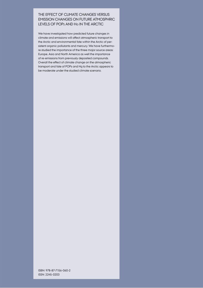
THE EFFECT OF CLIMATE CHANGES VERSUS EMISSION CHANGES ON FUTURE ATMOSPHRIC LEVELS OF POPS AND HG IN THE ARCTIC

We have investigated how predicted future changes in climate and emissions will aff ect atmospheric transport to the Arctic and environmental fate within the Arctic of per-sistent organic pollutants and mercury. We have furthermo-re studied the importance of the three major source areas: Europe, Asia and North America as well the importance of re-emissions from previously deposited compounds. Overall the eff ect of climate change on the atmospheric transport and fate of POPs and Hg to the Arctic appears to be moderate under the studied climate scenario.

ISBN: 978-87-7156-060-2ISSN: 2245-0203