School of Chemical Technology

Degree Programme of Chemical Technology

Jenni Ruohoniemi

THE EFFECT OF ADDITIVES ON ENZYME PARTICLE SIZE AND

DISTRIBUTION IN SPRAY DRYING

Master’s thesis for the degree of Master of Science in Technology

submitted for inspection, Espoo, 1st of August, 2016.

Supervisor Professor Alexander Frey

Instructor M.Sc. Arni Kujala

Aalto University, P.O. BOX 11000, 00076 AALTO

www.aalto.fi

Abstract of master's thesis

Author Jenni Ruohoniemi

Title of thesis The Effect of Additives on Enzyme Particle Size and Distribution in Spray Drying

Department Chemical Technology

Professorship Bioprocess Engineering Code of professorship Ke-70

Thesis supervisor Professor Alexander Frey

Thesis advisor(s) / Thesis examiner(s) M.Sc. Arni Kujala

Date 01.08.2016 Number of pages 83+45 Language English

Abstract

Enzymes and other products are dried to increase the storage life as liquid products are more vul-

nerable to contamination. Spray drying can be used to produce enzyme powders but they often con-

tain fine particles. Enzymes are allergenic and thus the smallest enzyme particles can cause perma-

nent health issues for employees exposed to them.

The aim of this study was to find ways to affect enzyme particle size by using additives as well as to

reduce or remove the smallest particles from the product.

The effect of sodium chloride on enzyme particle size was studied with three enzymes. In addition,

depending on the enzyme the use of sodium sulphate, calcium acetate, calcium chloride, methyl

cellulose, ascorbic acid and pH was studied.

The enzyme samples were spray dried with BÜCHI Mini Spray Dryer B-290. The particle size dis-

tribution and enzyme activity were measured for all the samples, and electron microscope pictures

were taken of chosen samples to receive more information.

There were significant differences between the particle size distributions of different enzymes. The

largest particle sizes were received with an enzyme that precipitated easily because of additives or

adjustment of pH. That enzyme also showed the greatest differences between the additives. Largest

particles were around 1000 µm in diameter formed of particles with a diameter of around 10 µm.

These kinds of particles are called agglomerates.

Agglomeration was discovered to be an important factor in the increase of the particle size and to

reduce the number of small particles. Even though it was possible to increase the mean particle size

by increasing the diameter of the particles, the differences were still significantly smaller compared

to those samples that had agglomeration.

A connection between enzyme precipitation and increased agglomeration was discovered but as there were many factors, of which several unknown, that affect the final product, the analysis of the results was complicated. In order to confirm the connection, repeating the experiments is necessary.

Keywords Spray drying, enzyme, additive, particle size distribution, agglomeration, precipitation

Aalto-yliopisto, PL 11000, 00076 AALTO

www.aalto.fi

Diplomityön tiivistelmä

Tekijä Jenni Ruohoniemi

Työn nimi Lisäaineiden vaikutus entsyymin partikkelikokoon ja -jakaumaan spray-kuivauksessa

Laitos Kemian tekniikka

Professuuri Bioprosessitekniikka Professuurikoodi Ke-70

Työn valvoja Professori Alexander Frey

Työn ohjaaja(t)/Työn tarkastaja(t) Arni Kujala

Päivämäärä 01.08.2016 Sivumäärä 83+45 Kieli Englanti

Tiivistelmä

Entsyymejä ja muita tuotteita kuivataan säilyvyyden lisäämiseksi, sillä nestemäisinä entsyymiliuokset ovat alttiimpia kontaminaatioille. Spray-kuivauksen tuloksena saadaan entsyymijauhetta, joka usein sisältää heinojakoisia partikkeileita. Entsyymit ovat allergeenisia, ja siksi pienimmät entsyymipartikkelit voivat aiheuttaa altistumisriskinsä vuoksi pysyviä terveyshaittoja työntekijöille. Tässä työssä tarkoituksena oli etsiä keinoja vaikuttaa entsyymien partikkelikokoon lisäaineiden avulla. Lisäksi pienimpien partikkelien poistaminen tai vähenteminen entsyymijauheista oli merkittävä käytännön tavoite. Työssä tutkittiin natriumkloridin vaikutusta kolmen eri entsyymin partikkelikokoon. Lisäksi entsyymistä riippuen tutkittiin natriumsulfaatin, kalsiumasetaatin, kalsiumkloridin, metyyliselluloosan ja askorbiinihapon sekä pH:n vaikutuksia. Entsyyminäytteet lisäaineineen kuivattiin BÜCHI Mini Spray Dryer B-290 –pöytäkuivurilla. Partikkelikokojakauma ja entsyymiaktiviisuus mitattiin kaikille jauhenäytteille ja lisäksi osa näytteistä analysoitiin elektronimikroskooppikuvien avulla. Entsyymien välillä huomattiin suuria eroja partikkelikokojakaumissa. Suurimmat partikkelikoot saatin entsyymillä, joka sakkautui lisäaineiden tai pH-olosuhteiden vaikutuksesta voimakkaimmin. Lisäaineiden välillä näkyi myös suurimmat erot kyseisellä entsyymillä. Suurimmat partikkelit olivat kokoluokkaa 1000 µm halkaisijaltaan. Ne olivat agglomeraatteja, eli ns. partikkeliryppäitä, jotka muodostuivat noin 10 µm halkaisijan partikkeleista. Agglomeraatio todettiin merkittäväksi tekijäksi pienten partikkelien vähentämisen kannalta. Vaikka keskimääräinen partikkelikoko saatiin kasvamaan ilman merkittävää agglomeraatiota, erot olivat suhteessa merkittävästi pienempiä kuin silloin kun parkikkelikoko kasvoi agglomeraation vaikutuksesta. Enstyymien sakkautumisen ja lisääntyneen agglomeraation välillä huomattiin yhteys, mutta monet tekijät vaikuttivat lopputuotteeseen vaikeuttaen tulosten analysointia. Toistojen vähyyden takia yhteyttä ei myöskään voitu todistaa.

Avainsanat Spray-kuivaus, entsyymi, lisäaine, partikkelikokojakauma, agglomeraatio,

saostuminen

Preface

The study was performed in Roal Oy in 2016. My advisor from the company was

their technical manager Arni Kujala and my supervisor from Aalto University was

professor Alexander Frey from the Department of Chemical Technology. The

experimental part was mostly performed in Formulation group in Roal lead by

Katja Palmunen.

The motivation for this study was to increase safety with enzyme powders by

reducing the number of small particles using additives in spray drying.

I want to thank you everyone who took part in my project and especially Arni

Kujala for advising, Katja Palmunen for helping with the experiments and

Alexander Frey for supervising.

I also want to thank you my family and friends who supported me through this

time and gave me strength and motivation to keep working.

The study was funded by Roal Oy.

Espoo 01.08.2016

Jenni Ruohoniemi

Contents

1 Introduction ................................................................................................................ 1

LITERATURE PART

2 Spray drying ................................................................................................................ 3

2.1 General ............................................................................................................ 3

2.2 Principle .......................................................................................................... 3

2.2.1 Feed ............................................................................................................. 4

2.2.2 Additives...................................................................................................... 4

2.2.3 Atomization ................................................................................................. 5

2.2.4 Evaporation ................................................................................................. 7

2.2.5 Gas separation ............................................................................................ 7

2.3 Parameters and their effects on the product ................................................. 8

2.4 Applications ................................................................................................... 11

2.4.1 Enzymes and other biological products .................................................... 11

2.4.2 Food industry ............................................................................................ 12

2.4.3 Pharmaceutical industry ........................................................................... 12

2.4.4 Others........................................................................................................ 13

3 Particle formation ..................................................................................................... 14

3.1 General .......................................................................................................... 14

3.2 Phenomena ................................................................................................... 14

3.2.1 Initial heating and evaporation ................................................................. 16

3.2.2 Particle formation and final drying ........................................................... 16

3.2.3 Interactions ............................................................................................... 17

3.3 Particle morphology ...................................................................................... 18

3.4 Particle size distribution ................................................................................ 20

4 Statistical analysis and hypothesis testing ................................................................ 21

4.1 General .......................................................................................................... 21

4.1.1 Statistic values........................................................................................... 21

4.1.2 Null and alternative hypothesis ................................................................ 22

4.1.3 Critical values and rejection area .............................................................. 23

4.1.4 p-value ....................................................................................................... 24

4.2 t-test .............................................................................................................. 25

4.3 χ2-test ............................................................................................................ 27

4.4 Regression analysis ....................................................................................... 28

4.4.1 Least squares method ............................................................................... 29

4.5 Correlation .................................................................................................... 30

EXPERIMENTAL PART

5 Aim ............................................................................................................................ 31

6 Materials and methods ............................................................................................. 31

6.1 Materials ....................................................................................................... 31

6.2 Equipment ..................................................................................................... 33

6.3 Methods ........................................................................................................ 33

6.3.1 Preparations .............................................................................................. 33

6.3.2 Spray drying .............................................................................................. 34

6.3.3 Analysis ..................................................................................................... 36

7 Results ....................................................................................................................... 39

7.1 Enzyme 1A ..................................................................................................... 39

7.1.1 Particle size distribution ............................................................................ 39

7.1.2 Scanning electron microscope (SEM) ........................................................ 42

7.1.3 Elemental analysis ..................................................................................... 43

7.1.4 Specific enzyme activity yield ................................................................... 43

7.2 Enzyme 1B ..................................................................................................... 44

7.2.1 Particle size distribution ............................................................................ 45

7.2.2 Scanning electron microscope (SEM) ........................................................ 47

7.2.3 Elemental analysis ..................................................................................... 48

7.2.4 Specific activity yield ................................................................................. 49

7.3 Enzyme 2 ....................................................................................................... 49

7.3.1 Particle size distribution ............................................................................ 49

7.3.2 Specific enzyme activity yield ................................................................... 50

7.4 Enzyme 3 ....................................................................................................... 51

7.4.1 Particle size distribution ............................................................................ 54

7.4.2 Scanning electron microscope (SEM) ........................................................ 57

7.4.3 Element analysis........................................................................................ 61

7.4.4 Specific enzyme activity yield ................................................................... 61

7.5 Material balance ........................................................................................... 65

7.6 Statistical analysis ......................................................................................... 67

7.6.1 Effect of calcium on particle size in Enzyme 3 .......................................... 67

7.6.2 Effect of calcium acetate on specific activity yield in enzyme 3 ............... 68

7.6.3 Protein concentration correlations ........................................................... 69

8 Discussion .................................................................................................................. 70

8.1 NaCl, Na2SO4 and pH ..................................................................................... 70

8.2 Methyl cellulose ............................................................................................ 72

8.3 Scale and fermentation differences .............................................................. 73

8.4 Reliability ....................................................................................................... 74

9 Conclusion ................................................................................................................. 74

10 Further studies ...................................................................................................... 75

References ........................................................................................................................ 76

APPENDICES

Appendix 1. Particle Size Distribution Curves

Appendix 2. Elemental Analysis Spectrums and Data

Appendix 3. Specific Enzyme Activity Yields

1

1 Introduction

Spray drying is an important drying method in many fields of industry, including

food, pharmaceutic and detergent industries. The history of spray drying goes

back to 1872 when Samuel Percy patented a method to dry and concentrate liquid

substances by atomization1, now also known as spray drying. Some decades later,

in 1920s, spray drying was first applied in the dairy and detergent industries2,3 and

in 1970s it became popular in instant coffee manufacturing4. Now, spray drying

has a variety of new applications3,5.

The great benefits of spray drying are that it is cost-effective compared to other

drying methods like freeze-drying6,7 and that the product stays at high

temperatures only for a short period of time leading to only minor undesired

reactions4. Therefore, spray drying suits heat-sensitive products too4.

An example of a temperature sensitive product is an enzyme, neglecting several

exceptions of enzymes that stay active in extreme conditions. At high

temperatures enzymes start to degrade and deactivate, and that is why traditional

methods like ovens do not offer an effective process. However, due to the speed

of the spray drying, it can be used to produce enzyme powder from liquid enzyme

solutions or suspensions4,8.

Even though spray drying seems to solve the problem of drying enzymes without

causing too much degradation and deactivation, another problem is faced with

the enzyme powder produced. The smallest enzyme powder particles are so small,

that they remain suspended in the air instead of settling on the floor where they

can be cleaned by vacuuming. As enzymes are allergenic and can cause health

issues for employees, lots of safety equipment is required. Separate rooms for

enzyme powder manufacturing help to reduce the area where the full set of safety

2

equipment is necessary, but working in that area is complicated and needs

education. If the smallest particles are removed from the product, the safety

increases for all the employees as risk of exposure to enzymes is reduced.

The aim of this thesis is to study the effect of additives on the particle size and

particle size distribution of enzymes in spray drying. Larger particle size along with

increased agglomeration helps to reduce the most problematic enzyme dust and

increase safety in enzyme powder manufacturing and research. Also, if the particle

size can be controlled, the product would be more homogeneous, thus improving

quality.

The Literature Part consists of three chapters: Spray drying, Particle formation,

and Statistical analysis and hypothesis testing. The chapter on spray drying

includes the different stages of the process, parameters and their effects, and

applications. The second chapter describes the phenomena of particle formation

and the methods to evaluate particles and their size distribution. The final chapter

in the Literature Part concentrates on statistical analysis and hypothesis testing in

order to explain the methods used to evaluate experimental data.

In the Experimental Part, spray drying of different products with several different

additives is described, analyzed and evaluated using statistical analysis methods.

Furthermore, the results from laboratory scale were compared to production scale

results in order to see how well the laboratory scale models the production scale.

The literature published on this topic is mostly from the food and pharmaceutical

industries. Especially in pharmaceuticals, the most common goal is to get smaller

particles with special morphology to help medicines to be absorbed by the body.

Studies on the effect additives have on the stability and morphology were

available but no studies examining the effect on particle size was found.

3

LITERATURE PART

2 Spray drying

This chapter is about spray drying, in order to give better understanding on the

unit operation for the reader. First, the general knowledge of spray drying is given.

Second, the principle of the drying process and its different stages are explained.

Third, the most important parameters and their effects on the product are

described. Finally, some of the most common applications are introduced.

2.1 General

Spray drying is a unit operation used to transform solutions or suspensions into

powders. It is a drying method where liquid is atomized and sprayed to a drying

chamber. In the chamber the moisture is removed by high rate evaporation.8-10

Even though high temperatures are used, spray drying can be applied to

temperature sensitive or unstable products without major losses of activity.

Therefore, enzymes and other biological products can be dried by spray drying.4

Another advantage in spray drying is that morphology of the particles can be

controlled by the feed solution characteristics and drying parameters11-13.

There are still challenges in spray drying. One major challenge is to optimize the

process for the product, as small variations of the feed solution can cause large

differences to the final product characteristics. Models and software have been

created to help to plan and optimize spray drying processes8,14-16.

2.2 Principle

The principle of the spray drying is simple. A feed solution is sprayed to a chamber

as small droplets. Drying gas then heats up the droplets and causes evaporation

and thus drying of the product.4 In this section, the steps of spray drying are

4

explained in more detail starting from the feed and proceeding through

atomization, evaporation and finishing with gas separation.

2.2.1 Feed

The feed solution has a high effect on the final product5. The particle size and

shape and other characteristics can vary remarkably depending on the dry mass

concentration, homogeneity, additives, or several other feed characteristics4,5.

The feed solution must be pretreated so that it does not contain unwanted

impurities or other components, as the drying process only removes the spare

solvent or water. Also, to receive homogeneous product, feed solution should be

homogeneous too.4

2.2.2 Additives

In order to get a product with desired properties, additives can be blended in the

feed solution. They increase the dry mass concentration as well as help to control

particle morphology and bulk density of the final product.4 Examples of additives

used in spray drying are salts like sodium chloride, polymers like maltodextrin or

gelatin, and proteins4,17.

Different additives are used for different purposes. Polymers like starches and

maltodextrins are used as additives due their high molar masses18,19. They can be

added to feed solution to increase the solids concentration, and thus improve the

drying process (see Table 1 in Section 2.3 for more information). They are efficient

in the cases where the product is amorphous with too low glass transition

temperature causing stickiness and caking19.

Another usage of additives is to precipitate the product. Salts can be used to

precipitate proteins, like enzymes or antibodies20,21. An antibody IgG was

5

precipitated by ammonium carbamate in order to increase protein stability during

spray drying20. Salts are also used to increase the solids concentration.

Additives are not always only helpful. The problem with maltodextrin, dextrin,

NaCl and Na2SO4 was noted by Sloth et al. They found that each of those additives

increased the droplet temperature. A problem occurred with higher additive

concentrations when a strong skin was formed. Instead of evaporation through

the pores of the skin, the inside of the droplet was gelatinized.22

Maltodextrin and dextrin were assumed to reduce the water activity by forming a

film on the surface of the droplet and salts by changing the chemical potential of

the droplet. As in high concentrations of these additives the resulting particles

were gelatinized, Sloth et al. suggested the usage of these additives improper for

temperature sensitive products.22

However, Gupta et al. proved that salts, polymers, sugars and sugar alcohols used

in their study actually increased the stability of xylanase enzyme. The specific

activity of the enzyme after spray drying was higher than without additives and

the half-life was also increased. There were differences between the additives, and

only several additives were chosen to be tested at different drying temperatures.

Tests suggested that by choosing an appropriate temperature and additives 99%

of activity could be retained through the spray drying process.21

2.2.3 Atomization

Atomization is the stage of drying where the droplets from the feed solution are

produced. The nozzle of the spray drier has a high effect on the mean droplet size,

and therefore on the particle characteristics of the product4,13,23. Four typically

used nozzle types are described in this section: two fluid nozzle, rotary disk

atomizer, pressure nozzle and ultrasonic nozzle (Figure 1).

6

Figure 1. Different types of nozzles for spray drying exist and the spray produced

depends on the nozzle characteristics. A) Two fluid nozzle B) Rotary disk atomizer

C) Pressure nozzle D) Ultrasonic nozzle.4

Two fluid nozzles are commonly used in research6,16,18,21. The energy for

atomization is provided by the spray gas mixed with the feed solution. When the

gas-liquid mixture enters the drying chamber, the gas expands rapidly and

produces droplets. The droplet size can be controlled by the gas-liquid mass ratio:

higher gas ratio (>3:1) results smaller droplets (5-20 microns) and smaller ratio

(0.5:1) larger droplets (125 microns).4

Rotary disk atomizers spray the feed solutions into the drying chamber as a fine

mist that is dried by a concurrently flowing gas. The benefit of the rotary disks is

that they provide high feed throughput, which makes them applicable in industrial

scale. The droplet size is controlled by the peripheral velocity of the disks, where

higher velocity (>180 m/s) causes smaller droplets (20-40 microns) and lower

velocity (75 m/s) larger droplets (225 microns).4

Pressure nozzles are used if large droplets are wanted. The pressure provided

creates a thin film of the feed which enables drying of larger particles. The particle

size depends on the feed rate and viscosity, but the mean particle size is controlled

by the pressure. Lower pressure, around 15-25 bars creates larger droplets in the

range of 150-350 microns while over a 100 bar pressure creates droplets of around

20-40 microns.4

7

Ultrasonic nozzles control the droplet size by frequency of the nozzle vibration.

Surface tension and viscosity of the feed solution also have an effect on droplet

size.4 This technique gives highly uniform droplets, which makes it important in

the research of particle size and morphology12. However, the largest droplets

produced by the ultrasonic nozzle are only around 70 microns (25 kHz) and

smallest 18 microns (120 kHz), which is relatively narrow range compared to the

others nozzles introduced.4

2.2.4 Evaporation

When liquid droplets come into contact with the spray gas, evaporation begins on

the droplet surface immediately4. The spray gas can be air, an inert gas like

nitrogen or argon, or steam4,13. Due to the high surface area of small droplets both

heat and mass transfer are intensive and result an efficient drying4,8. The

evaporation phenomenon is explained in more detail in Section 3.2.

To understand the evaporation stage, basic knowledge on evaporation is required.

Phase change from liquid droplet to gas requires energy and that energy is taken

from the spray gas. When biological products are spray dried, it is important to

work at low temperatures (inlet temperature 145-160 °C, outlet temperature <80

°C)10,24. Inlet temperature cannot be decreased too much as the moisture content

of the product has to stay low (<6 %). By increasing the feed rate, outlet

temperature decreases as more energy from the spray gas is required to

evaporation of solvent from droplets. Reduced energy in spray gas causes

decreased outlet temperature. More about parameters and their effects in spray

drying is described in Section 2.3.

2.2.5 Gas separation

Before the final product is received, the gas must be separated. Examples of

separators are a cyclone (Figure 2)4, filter bag and electrostatic precipitator3. In

the cyclone, the solid particles flow to the bottom of the device where a collection

8

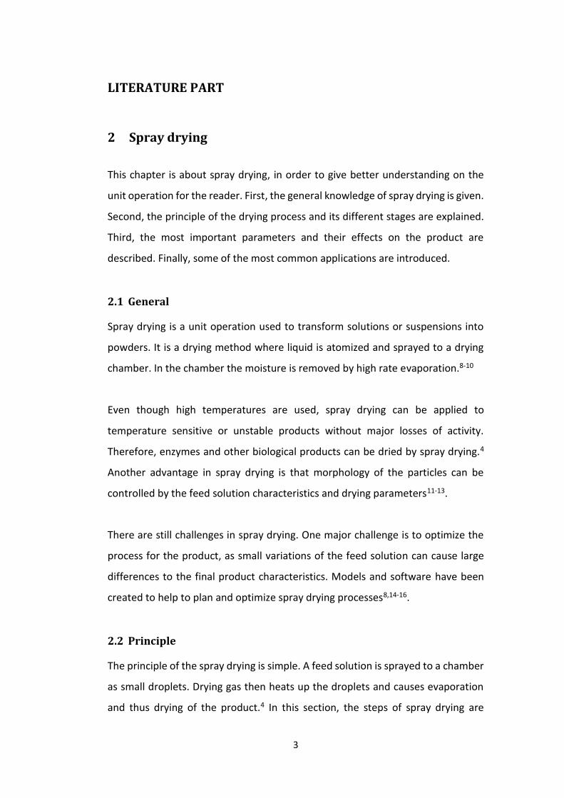
dish is connected and the gas flows out from top. In order to ensure that no solid

particles stay in the gas, a filter can be used after the cyclone.

Figure 2. A cyclone (front) can be used to separate gas and solid product in spray

drying. To ensure solid-free gas release, a filter can be connected in series after

cyclone (back).4

2.3 Parameters and their effects on the product

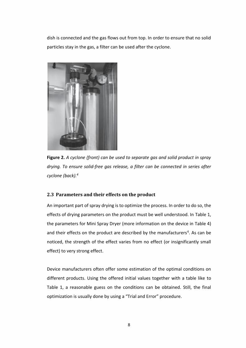
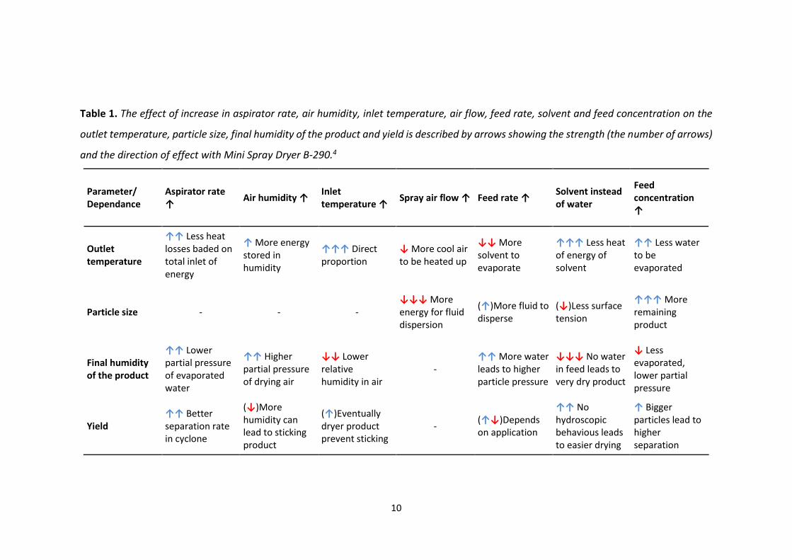
An important part of spray drying is to optimize the process. In order to do so, the

effects of drying parameters on the product must be well understood. In Table 1,

the parameters for Mini Spray Dryer (more information on the device in Table 4)

and their effects on the product are described by the manufacturers4. As can be

noticed, the strength of the effect varies from no effect (or insignificantly small

effect) to very strong effect.

Device manufacturers often offer some estimation of the optimal conditions on

different products. Using the offered initial values together with a table like to

Table 1, a reasonable guess on the conditions can be obtained. Still, the final

optimization is usually done by using a “Trial and Error” procedure.

9

For heat sensitive products like enzymes and other biotechnological products, the

temperature is one of the most important variables. In order to avoid deactivation

and degradation of the product the parameters affecting it must be controlled.

The most effective way to control outlet temperature is to control inlet

temperature (Table 1).

10

Table 1. The effect of increase in aspirator rate, air humidity, inlet temperature, air flow, feed rate, solvent and feed concentration on the

outlet temperature, particle size, final humidity of the product and yield is described by arrows showing the strength (the number of arrows)

and the direction of effect with Mini Spray Dryer B-290.4

Parameter/ Dependance

Aspirator rate ↑

Air humidity ↑ Inlet temperature ↑

Spray air flow ↑ Feed rate ↑ Solvent instead of water

Feed concentration ↑

Outlet temperature

↑↑ Less heat losses baded on total inlet of energy

↑ More energy stored in humidity

↑↑↑ Direct proportion

↓ More cool air to be heated up

↓↓ More solvent to evaporate

↑↑↑ Less heat of energy of solvent

↑↑ Less water to be evaporated

Particle size - - - ↓↓↓ More energy for fluid dispersion

(↑)More fluid to disperse

(↓)Less surface tension

↑↑↑ More remaining product

Final humidity of the product

↑↑ Lower partial pressure of evaporated water

↑↑ Higher partial pressure of drying air

↓↓ Lower relative humidity in air

- ↑↑ More water leads to higher particle pressure

↓↓↓ No water in feed leads to very dry product

↓ Less evaporated, lower partial pressure

Yield ↑↑ Better separation rate in cyclone

(↓)More humidity can lead to sticking product

(↑)Eventually dryer product prevent sticking

- (↑↓)Depends on application

↑↑ No hydroscopic behavious leads to easier drying

↑ Bigger particles lead to higher separation

11

2.4 Applications

Spray drying is a widely used drying method in several fields of industry. In this

section some of its most common applications in the product formulation in

biotechnological, food and pharmaceutical industries are introduced as well as

several others including detergents and nanoparticles.

2.4.1 Enzymes and other biological products

Drying is an efficient method to increase shelf-life of biological products like

enzymes and other proteins25. There are several drying methods available, but

spray drying enables efficient drying without major losses in activity if the

parameters are correctly chosen.4,24

For efficient drying with high enzyme activity preservation the choice of drying

parameters is important10,24. The preservation of enzyme activity is of course

important as generally enzymes and other biological products are produced

because of their biological activity.

In addition to drying parameters, use of additives can help to stabilize the product.

There are significant differences in results between studies of different enzymes

and other biological products.21,26,27 For example, Selianov noticed that some

common salts were not effective stabilizers for cellulases, but instead, different

forms of cellulose were26. In contrast, Gupta found out that many salts are

effective stabilizers for xylose, and that using salts together with polyols or

polymers, the effect can be enhanced remarkably21.

One reason for the differences in the stabilizing effects is the differences in the

additive function. Salts can be used to precipitate the enzyme and that way protect

it during spray drying20. Maltodextrin can be used to immobilize the enzyme, and

12

sugars like trehalose to encapsulate, and thus, protect the enzyme21,28,29. In some

cases, polyols like sorbitol are used to avoid aggregation27.

In order to use proper drying parameters and additives for the products, the

stabilizing effects of different additives on the enzyme or other biological products

must be understood. There are some publications available, but only with the

most common products and additives.10,21,24,26,27

2.4.2 Food industry

In 1920s, milk powder was produced for the first time. It was the first time spray

drying was used in food industry, and together with detergent industry, the first

commercial application of spray drying2,3.

Milk is dried to increase its shelf-life and to reduce transportation and storage

costs. Also, milk powder is easy to use in food industries that use milk as raw

material.16,30 An important factor to evaluate the milk powder quality is the

moisture content, and there are standards for the highest acceptable moisture

levels16.

Currently, spray drying is used for several food products including egg products,

beverages, vegetable proteins, fruit and vegetable extracts, carbohydrates, tea

extracts and yogurt, among others3,17,18,31,32.

2.4.3 Pharmaceutical industry

Spray drying has become of great interest in the pharmaceutical industry. The

increased control of morphology and particle size enables the production of new

formulation of drugs. For example, oral drugs could be replaced by inhalable drugs

as they often require lower dosage.33-35

13

In many cases, carriers are used to transport the drug. By using additives and

controlling the parameters of spray drying, the morphology of the drug can be

modified so that carriers are no longer necessary33. This way long storage times

will not affect the adhesion characteristics between the drug and carrier, and

therefore the effectiveness of the drug36.

Even though many products are still at the theoretical or experimental stage, there

are already several pharmaceuticals produced using spray drying34.

2.4.4 Others

In addition to biological products, food and pharmaceutical industries, there are

many other applications for spray drying. In this section, only detergents and

nanoparticles are introduced, but spray drying is used in chemical industry in

production of catalysts, dyes and several other products5.

Detergents were produced by spray drying already in 1920s2,3. As the technology

is widely used, there are not many recent studies on topic available. Furthermore,

some standardized systems have been developed and used all over the world.37

Nanoparticles can also be produced by spray drying. The advantage of using spray

drying is that higher concentrations of reacting species can be used compared to

other methods like precipitation methods or reversed micelles.5 There are several

studies on how to produce desired kind of particles by spray drying, as in

nanotechnology, the morphology and particle size distribution are important for

the applications. Nanoparticles can be used in electronics, optics, sensors, and

drugs, among others.5,11-13,23,38

14

3 Particle formation

In this chapter, the particle formation is discussed in greater detail. First, general

information on particle formation is given. Second, the phenomena behind the

particle formation from droplet, and interactions are explained. Third, the particle

morphology is introduced in order to better understand the drying process, and

finally the particle size distribution and how to measure it is explained.

3.1 General

Solid particles form during the evaporation stage of the spray drying (Section

2.2.4)4. They differ in many ways including size, moisture content and shape, but

also by their homogeneity, charge, bulk density and ability to agglomerate4,39.

Depending on the particle application, different characteristics are important. In

case of enzymes and other biomaterials, it is important that the final product is

still active and that the moisture content is low enough to improve storage life25.

3.2 Phenomena

Droplet transformation into a particle is a widely studied phenomenon, starting in

the 1950s, when Ranz and Marshall first described evaporation from droplet. In

2015, Mezhericher et al. reviewed all the stages of drying, in order to create a

software to simulate and model spray drying.8,38,40

Figure 3 shows the basic idea of droplet transformation into a particle in the spray

drying process. First, the droplet is heated to its evaporation temperature

followed by evaporation of the surface layer. Second, a skin is formed around the

droplet transforming it to a wet particle. Last, the wet particle dries and is heated

to surrounding temperature.

15

Figure 3. Droplet temperature varies at different stages of drying. Solid line:

suspension, dash line: solution8

Temperature of the droplet varies during the drying and it depends on the feed

solution characteristics. For solutions, temperature rises quite smoothly during

the whole drying time, whereas for suspensions clear steps for initial heating,

evaporation and particle drying can be seen (Figure 3).8 This is due to differences

in evaporation process. Dissolved materials like salts change the evaporation

temperature of the solution compared to pure water. When the water evaporates,

the salt concentration increases and causes the evaporation temperature to

increase too. This is why there is no stage with a constant temperature.

Unlike solutions, suspensions consist of two or more phases. One phase does not

affect the evaporation temperature of the other phase, so when the temperature

16

reaches the evaporation temperature of water, it stays constant until the skin is

formed which starts to disturb the evaporation.41

3.2.1 Initial heating and evaporation

The first step in particle formation is the initial heating of the droplet to its

equilibrium evaporation temperature. The equilibrium evaporation temperature

is defined where the droplet surface temperature stays constant.8 In this

equilibrium state, the energy provided by the drying gas and the energy needed

for the evaporation from the droplet surface are equal.

However, depending on the droplet characteristics, the temperature might not

have an equilibrium evaporation temperature. Thus, different equations and

models apply to solutions and suspensions8,38. However, in the simplest case the

evaporation happens on the droplet surface, the droplet shrinks and gets more

concentrated8. Eventually, the solid concentration on the surface is so high that a

skin, or crust is formed8,39.

In most cases, the process is more complicated and many variables have to be

included. Some factors like density and specific heat capacity are functions of

temperature. Especially during the initial heating and evaporation, when the

temperature is not constant, this temperature dependence has to be taken into

account. Because the equations are complicated, technology can be a great help

in calculations or modeling of process.8

3.2.2 Particle formation and final drying

Particle formation starts in the end of evaporation stage, when a skin around the

droplet is formed. Then the droplet is called a wet particle. However, the

transformation is not always immediately completed after skin formation.8 The

initial skin might not be strong enough and collapses due to compressive capillary

forces caused by the higher pressure outside of the droplet14. Then the

17

evaporation continues until a new skin is formed. This may happen several times

before the final, stable skin is formed. This stage is called transition period.8,14

According to Mezhericher et al. the particle drying happens by vapor diffusion

through the pores in the skin8. The temperature of the particle increases as the

moisture content decreases until the particle is dry and reaches the temperature

of the environment (Figure 3).

3.2.3 Interactions

Although the studies on the particle formation increase the understanding of the

drying phenomena, often systems with only one droplet or particle are

studied8,9,40. However, the spray drying process involves a great number of

droplets and particles that interact.

Droplets interact by droplet-droplet collisions. The type of collision can be a

bounce, coalescence or breakage of the colliding droplets. A bounce causes the

change of velocity and direction of the droplet. This can affect the evaporation

from the droplet surface.8

Droplets may combine and form larger droplets, or break into smaller droplets by

collision.8 The change in droplet diameter has a significant effect on the drying

process making it faster or slower. Smaller droplets dry faster than larger droplets

due to larger surface to volume ratio, and the rate of drying affects the

morphology, among other characteristics8,39.

In addition to droplets, particles can also interact by collisions8,39. The type of

collision depends on the particles, as hard-spheres are more probably bouncing

than breaking up, but hollow particles may break. Also the moisture content of the

particles has an effect on the interactions as wet particles may combine and cause

agglomerates39.

18

In the spray drying process, droplets and particles also collide with the walls of the

drying chamber8. Those collisions can cause chamber fouling, and thus, decrease

the yield42. Dry and crystalline particles do not stick to chamber wall as easily as

wet particles, and droplet-wall collisions can be reduced by adjusting the nozzle

so that the feed does not touch the walls before it dries42,43.

3.3 Particle morphology

Particle morphology describes the shape of the particle. The shape can be dense

spherical, hollow, doughnut shaped, encapsulated, hairy or porous, among others

(Figure 4). There are several studies on particle morphology in spray drying on how

to receive certain type of particles5,13,23,39. As the nanoparticle morphology plays

an important role in many applications, like drug carriers in the pharmaceutical

industry and superconductors in electronics, the development of methods to

produce particles with desired morphology are of great interest5,23.

From Figure 4 it can be noticed that the particle types can be divided into two

groups. There are particles formed of one component only and particles formed

of two components (composite particles). Some of the structures are formed in

several steps like the formation of porous particles.13

19

Figure 4. Particles from spray drying can have different morphologies depending

on how they were dried.13

When a solution with only one component is spray dried, dense, hollow or

doughnut particles can be formed from the same solution by varying the drying

parameters13,44. When the evaporation rate of a droplet is low the result is a dense

particle, whereas with high evaporation rates the particle is hollow44. If the drying

gas flow or the drying temperature in the chamber is increased, particles are

destabilized and change morphology from spherical to “mushroom hat” towards

the doughnut shape11. An example of a single component solution is an inorganic

solution used in the production of nanoparticles13.

Two-component solutions form either encapsulated or well-mixed particles

depending on the particle size difference of the two components. If they are of

equal size, well-mixed particles are formed.13

20

Depending on the particle characteristics or state of drying (i.e. the moisture

content), agglomeration may occur. The main reasons for agglomeration

according to Walton and Mumford are the moisture content and static electrical

effects39.

3.4 Particle size distribution

The product of spray drying is not homogenous, but instead, the particles vary in

size4. The feed solution properties and drying conditions have an effect on the final

particle size distribution, and by understanding the effects the distribution can be

modified into a desired direction24,45,46.

Narrow distribution means that the product is close to homogeneous in particle

size. This is a desired characteristic in many fields of study and industry as the

applications often require homogeneity in order to create products with high

quality5,23,44.

Particle size distribution can be measured by devices designed for that. Several

different methods are used for the detection of the particle size depending on the

size range47. A common method with a wide size range is laser diffraction. Other

methods include dynamic light scattering, resonant mass measurement, and

Raman or imaging47,48.

21

4 Statistical analysis and hypothesis testing

In the evaluation of experimental data and its reliability, statistical analysis and

hypothesis testing are useful tools. This chapter introduces the most important

statistic values and several commonly used hypothesis testing methods.

4.1 General

Statistical analysis is based on the collected data and its statistics. Some of the

most important statistics are means and variances, along with standard deviation

and covariance. With the help of estimators, the experimental data can be used

to evaluate the hypothesis. There exist several ways to execute hypothesis testing,

of which t-test and χ2-test can be used in a variety of applications.49,50

Also, several ways to evaluate the data by hypothesis testing exist. Hypothesis

testing is based on critical values and rejection area or the p-value. Those values

help to either accept or reject the hypothesis.49

4.1.1 Statistic values

While there are several different types of means and variances, the most common

to this work are the arithmetic mean, X̅ or x̅, and the sample variance, s2. The

equation for x̅ is described below in the Equation 1, and Equation 2 describes the

sample variance:

�̅� =1

𝑛∑ 𝑥𝑖

𝑛

𝑖=1

(1)

𝑠2 =1

𝑛 − 1∑(𝑥𝑖 − �̅�)2

𝑛

𝑖=1

(2)

22

where n is the number of samples, xi is the value of ith sample.49

The expected value, E(X), is the value of the discrete random variable X that is most

probably the mean of X. The variance of X is sometimes denoted as Var(X). This

notation helps to differentiate variances of different variables as variance can be

calculated to arithmetic mean or other estimators. An expected value denoted as

μ refers to an expected value using normally distributed density function N and σ2

to the variance of N. 49,51

Standard deviation is the square root of variance, denoted as σ or sx. Standard

deviation of the sample means is also called the standard error of the estimate.

49,50

Variance is a special case of covariance. Covariance describes how two different

random variables change together. That information can be used in the evaluation

of regression lines to test linear correlation between plotted data points. Equation

3 is used to calculate the covariance.

𝑆𝑥𝑦 =1

𝑛∑(𝑥𝑖 − �̅�)(𝑦𝑖 − �̅�)

𝑛

𝑖=1

(3)

where n is the number of samples, xi and yi are the values of ith samples and x̅ and

y̅ are the arithmetic means. 50

4.1.2 Null and alternative hypothesis

Hypothesis testing can be used to evaluate data and is widely applied in statistical

analysis. In order to understand different tests introduced in Sections 4.2 and 4.3,

some basics of hypothesis testing should be explained.

23

Hypothesis testing starts with a general hypothesis often denoted as H. H defines

the variables of the test. After that a null hypothesis is defined and denoted as H0.

In its simplest form H0 can be defined as “equals”. For example with a discrete

density function f(x;θ), where x is a data point and θ is an unknown parameter,

null hypothesis can simply have a form

H0: θ = θ0 (4)

where θ0 is the expected value of the parameter θ according to the H0. Hypothesis

testing can be used to evaluate calibration (

H0: μ = μ0, where μ0 is the expected mean) or correlation (Section 4.5), to

mention a few applications. In the case that H0 does not apply, the alternative

hypothesis H1 comes into effect. H1 is also defined before the actual hypothesis

testing. In the case of Equation 4, H1 can be defined according to Equations 5, 6

and 7. 49

H1: θ < θ0 (5)

H1: θ > θ0 (6)

H1: θ ≠ θ0 (7)

4.1.3 Critical values and rejection area

After defining a null and an alternative hypothesis a rejection area must be

defined. A significance level α is chosen and is a probability for a test variable to

be in the rejection area. Common significance levels are 0.05, 0.01 and 0.001.

Using statistical tables, critical values for the test variables can be found. 49,52

As an example for finding the rejection area, the hypotheses defined in Equations

4 and 5 are used. For Equation 5 the rejection area for test variable distribution Z

is defined by the following Equation 8:

24

Pr(𝑍 ≤ 𝑙|H0) = α (8)

where l is the critical value for the test variable. See the Figure 5 for a graphical

representation. 49

Figure 5. Test variable density function with a significance level α and a critical

value l. The values equal to or smaller than l are in the rejection area and the null

hypothesis does not apply.

4.1.4 p-value

Another way to make decisions whether to accept the null hypothesis is to use p-

values. The p-value is a probability that a test variable gets an improbable value

even if the null hypothesis applies. A small p-value is defined and denoted as p0.

Using statistical tables, the p-value for the test variable can be calculated. If p is

smaller than p0, then the null hypothesis most probably does not apply and the

alternative hypothesis comes into effect. The following Equations 9, 10 and 11 can

be used to calculate p-values for the hypotheses used previously in Equations 5, 6

and 7, respectively.

25

𝑝 = Pr (𝑍 ≤ 𝑧|H0) , (9)

𝑝 = Pr(𝑍 ≥ 𝑧|H0) and (10)

2𝑝 = Pr (𝑍 ≥ |𝑧||H0) . (11)

where z is the test variable calculated from the data and H0 is the null hypothesis

from Equation 4. 49

4.2 t-test

t-test is a commonly used test for hypothesis testing for an expected value. It can

be used to test one random variable or to simultaneously test two unrelated

random variables for agreement with the hypothesis. Additionally the t-test can

be used to compare values of pairs.49

For perferming t-test, several assumptions are made. The mean of the collected

data is assumed to follow a normal distribution density function N with known μ

and σ2 50. For evaluation of one or two random variables, sample mean X̅ and

sample variance s2 must be calculated using Equations 1 and 2. Then the t-value

can be calculated. For one random variable,

𝑡 =�̅� − 𝜇0

𝑠

√𝑛

(12)

where X̅ is the sample mean, μ0 is the expected value, s is the standard deviation

and n is the sample size. There are (n − 1) degrees of freedom.49,50 The number of

degrees of freedom is the number of values that can vary without affecting the

system. Often the degrees of freedom are defined as the number of data points

subtracted by the number of parameters.53

26

The rejection area and critical values can be calculated as in Section 4.1.3 and then

t-value calculated from Equation 12 can be compared to critical values received

from statistical tables.49,52

For two random variables the t-value can be calculated using either Equation 13

or Equation 14 depending on the variance. If variances of random variables are

different, Equation 13 is used.49

𝑡𝐴 =

�̅�1 − �̅�2

√𝑠1

2

𝑛1+

𝑠22

𝑛2

(13)

If variances of random variables are the same, Equation 14 is used.49

𝑡𝐵 =

�̅�1 − �̅�2

𝑠𝑝√1𝑛1

+1

𝑛2

(14)

where sp is a pooled variance:

𝑠𝑝 =(𝑛1 − 1)𝑠1

2 + (𝑛2 − 1)𝑠22

𝑛1 + 𝑛2 − 2 (15)

Degrees of freedom are easy to define for tB as it is simply (n1 + n2 − 2), but for

tA approximations must be used. One example is the Satterthwaiten

approximation (Equation 16) which is rounded down to the closest full number.49

𝑣 =(

𝑠12

𝑛1+

𝑠22

𝑛2)

2

1𝑛1 − 1 (

𝑠12

𝑛1)

2

+1

𝑛2 − 1 (𝑠2

2

𝑛2)

2 (16)

27

Pair comparison is used for data where experimental data is formed from pairs

and it can be used if there are two identical experiments done, among other cases.

The difference between data pairs (Di) is used for the calculations. The sample

mean, sample variance and t-value are calculated using Equations 17−20.49

𝐷𝑖 = �̅�1 − �̅�2 (17)

�̅� =1

𝑛∑ 𝐷𝑖

𝑛

𝑖=1

(18)

𝑠𝐷2 =

1

𝑛 − 1∑(𝐷𝑖 − �̅�)2

𝑛

𝑖=1

(19)

𝑡 =�̅�𝑠𝐷

√𝑛

(20)

4.3 χ2-test

χ2-test is a commonly used test when the expected value μ is unknown but the

variance is known for a random variable.49 The test begins with defining the

hypotheses.

General hypothesis H is that discrete random variable X has μ and σ2 following the

normal distribution N, i.e., Xi~N(μ, σ2). The null hypothesis H0 is

H0 ∶ 𝜎2 = 𝜎02 (21)

where σ02 is the expected variance.49

Arithmetic mean and sample variance for X can be calculated using Equations 1

and 2. Knowing them, a test variable χ2 can be calculated using Equation 22.

28

𝜒2 =(𝑛 − 1)𝑠2

𝜎02 (22)

where (n − 1) are the degrees of freedom. If H0 is valid,

𝐸(𝜒2) = 𝑛 − 1 (23)

This means that both large and small values of χ2 suggest that null hypothesis

should be rejected. The rejection area and p-value can be found similarly as

described in Sections 4.1.3 and 4.1.4.49,50

4.4 Regression analysis

Regression analysis is the most commonly used and applied method in statistical

analysis. It concentrates on explaining the relationship between variables of

measured data. Regression analysis explains the strength of the relationship as

well as helps to predict the results of further experiments, and can be used to

create a regression model.49

Regression models can be divided into linear and nonlinear functions. Evaluation

of nonlinear models is challenging, so it is recommended to linearize the model

and use regression analysis for the linearized model.49,50 A linearized model can

either be a deterministic model or regression function. They have similarities but

they are based on different ways to treat the data.

A deterministic model is used to define the relationship between the variables

using observations by looking for a model that best fits to data points. It is often

in the form of Equation 25. A regression function (Equation 26) is the conditional

expected value of y as a function of conditional variable x. So the function is

defined so that the expected value of y can be predicted as well as possible using

values of x.

29

𝑦 = 𝑓(𝑥 ; 𝛽) (24)

𝐸(𝑦|𝑥) = 𝑓(𝑥 ; 𝛽) (25)

where y is a variable, x is the determining variable and β is an unknown parameter

that determines the shape of the function f. If a value for β can be found and it is

always constant, the function is fully determined. This is, however, rarely the

situation. In order to solve the problem, the equations are rewritten into the form

of Equation 26.49

𝑦𝑖 = 𝑓(𝑥𝑖 ; 𝛽) + 𝜀𝑖 (26)

where εi is the residual term varying in each observation unit. To get the best

fitting function for the model, β should be chosen so that εi is as small as possible

for each observation.49 One method to solve the value of β is to use the least

squares method described in Section 4.4.1.49,50

4.4.1 Least squares method

Least squares method is a method to solve regression problems mentioned in

Section 4.4.49,50 It is based on finding the smallest square sum of residual term εi

of a linear regression function in respect to regression factors β0, β1, … , βk.

∑ 𝜀𝑖2 = ∑(𝑦𝑖 − 𝛽0 − 𝛽1𝑥𝑖1 − 𝛽2𝑥𝑖2 − ⋯ − 𝛽𝑘𝑥𝑖𝑘)2

𝑛

𝑖=1

𝑛

𝑖=1

(27)

The minimal value of ∑ εi2n

i=1 in Equation 27 is generally done by derivation. The

solutions for β0, β1, … , βk are estimators often denoted as b0, b1, … , bk.49 Different

computer programs can be used to calculate the estimators and find the

regression function, and therefore help to evaluate the data.

30

4.5 Correlation

Correlation describes the statistical dependence of two variables. For linear

correlation, dependence can be evaluated by using correlation coefficient, rxy. The

equation for the calculation of the correlation coeffiecient is described below in

Equation 28.49,50

𝑟𝑥𝑦 =𝑆𝑥𝑦

𝑆𝑥𝑆𝑦 (28)

where Sxy is the covariance of x and y of the data according to Equation 3, Sx and

Sy are the standard deviations of standard variances of x and y of data according

to Equation 2.

The values of rxy vary between ±1, where positive value means positive slope of

regression line and vice versa. Values of |rxy| close to 1 mean strong linear

dependence of the data points, and values close to 0 mean no linear correlation.

However, that does not mean no dependence as the dependence can be

nonlinear.49,50

The correlation coefficient can also be used for nonlinear dependence, but only if

the dependence can be linearized by axis transformation.50

For evaluation of correlation, t-test in Section 4.2 can be used. One way is to set

the null hypothesis

H0 ∶ 𝜌𝑥𝑦 = 0 (29)

where ρxy is the correlation of the variables x and y. In this case there exists no

linear correlation if H0 applies.49

31

EXPERIMENTAL PART

5 Aim

The aim of this study was to study the effect of additives on enzyme particle size

in spray drying and removing the smallest particles (diameter <10 µm) using

particle size distribution analyzer and SEM to determine the particle size. The

chosen additives were salts like sodium chloride, sodium sulphate, calcium acetate

and calcium chloride, and methyl cellulose. Their effect on particle size was

studied using three different enzyme solutions.

The three enzyme solutions were chosen so that the differences between the

effects of additives on different enzymes could be compared.

Statistical analysis methods were used to analyze the statistical reliability of the

resulting data, correlations and conclusions drawn from them.

6 Materials and methods

In this chapter, the materials, equipment and methods used in the study are

described.

6.1 Materials

The enzyme solutions used are named as 1A and 1B, 2, and 3 where numbering

refers to different enzymes, and A and B to same enzyme produced by different

strains (Table 2). The samples of enzyme 3 consisted of three different batches,

one from production scale and two from pilot scale. They were named as 3.1, 3.2

and 3.3, respectively.

32

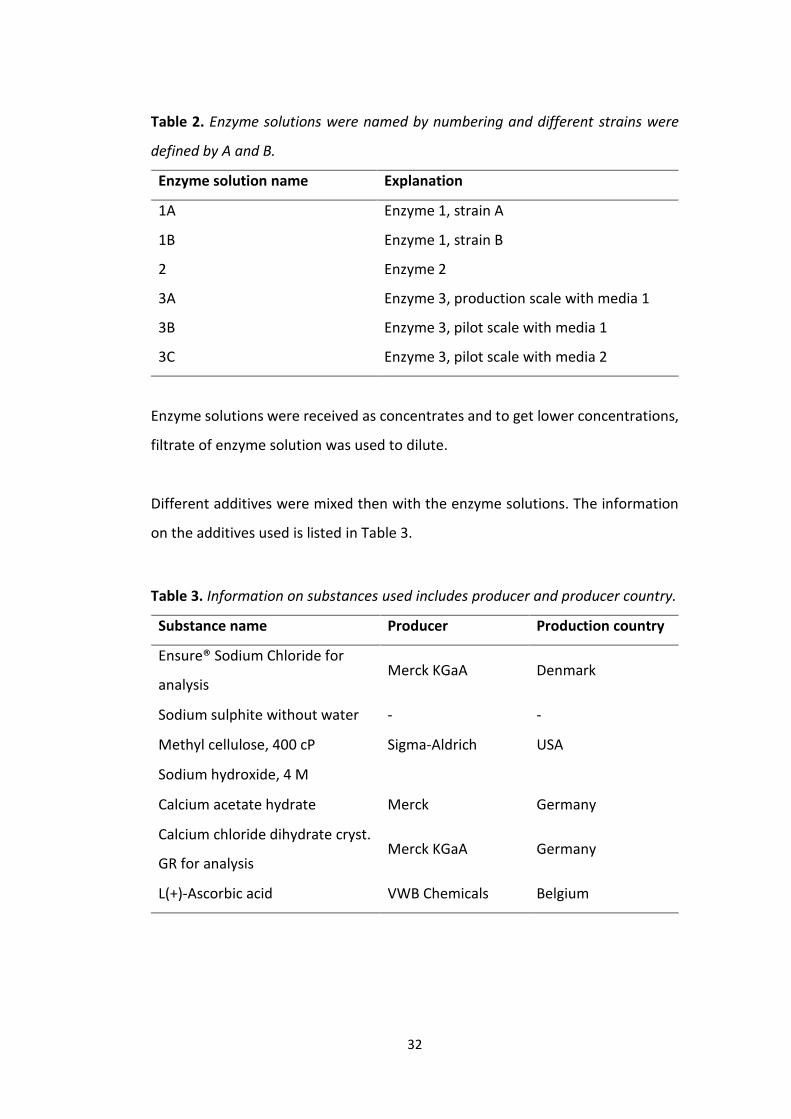
Table 2. Enzyme solutions were named by numbering and different strains were

defined by A and B.

Enzyme solution name Explanation

1A

1B

2

3A

3B

3C

Enzyme 1, strain A

Enzyme 1, strain B

Enzyme 2

Enzyme 3, production scale with media 1

Enzyme 3, pilot scale with media 1

Enzyme 3, pilot scale with media 2

Enzyme solutions were received as concentrates and to get lower concentrations,

filtrate of enzyme solution was used to dilute.

Different additives were mixed then with the enzyme solutions. The information

on the additives used is listed in Table 3.

Table 3. Information on substances used includes producer and producer country.

Substance name Producer Production country

Ensure® Sodium Chloride for

analysis Merck KGaA Denmark

Sodium sulphite without water - -

Methyl cellulose, 400 cP Sigma-Aldrich USA

Sodium hydroxide, 4 M

Calcium acetate hydrate Merck Germany

Calcium chloride dihydrate cryst.

GR for analysis Merck KGaA Germany

L(+)-Ascorbic acid VWB Chemicals Belgium

33

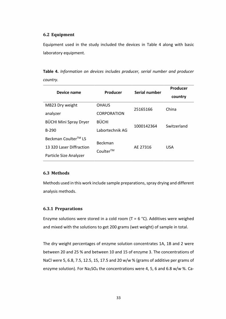
6.2 Equipment

Equipment used in the study included the devices in Table 4 along with basic

laboratory equipment.

Table 4. Information on devices includes producer, serial number and producer

country.

Device name Producer Serial number Producer

country

MB23 Dry weight

analyzer

OHAUS

CORPORATION 25165166 China

BÜCHI Mini Spray Dryer

B-290

BÜCHI

Labortechnik AG 1000142364 Switzerland

Beckman CoulterTM LS

13 320 Laser Diffraction

Particle Size Analyzer

Beckman

CoulterTM AE 27316 USA

6.3 Methods

Methods used in this work include sample preparations, spray drying and different

analysis methods.

6.3.1 Preparations

Enzyme solutions were stored in a cold room (T = 6 °C). Additives were weighed

and mixed with the solutions to get 200 grams (wet weight) of sample in total.

The dry weight percentages of enzyme solution concentrates 1A, 1B and 2 were

between 20 and 25 % and between 10 and 15 of enzyme 3. The concentrations of

NaCl were 5, 6.8, 7.5, 12.5, 15, 17.5 and 20 w/w % (grams of additive per grams of

enzyme solution). For Na2SO4 the concentrations were 4, 5, 6 and 6.8 w/w %. Ca-

34

acetate and CaCl2 were at 2 w/w % concentration, methyl cellulose at 1.5 w/w %,

and ascorbic acid at 0.5 w/w %.

If the enzyme solutions were diluted, it was done 1:1 (concentrate : filtrate) and

named as mix. Thus, the concentrations of the enzyme solutions can be defined as

concentration factors. For filtrate the concentration factor is 1, for mix it is 1+𝑋

2,

and for concentrate it is X. If for example the concentration factor for the

concentrate is 2, then for the mix it is 1.5.

The pH of several samples was adjusted and it was performed after addition of

other additives using 4 M NaOH solution.

If the sample was not spray dried immediately, it was stored in the cold room. Also

if the additive did not dissolve easily or precipitated so that mixing would not make

the solution homogeneous again after storage, solution was stored under mixing.

6.3.2 Spray drying

Before drying, the spray dryer (Table 4) was prepared and the drying parameters

were set. The parameters used depended on the type of cyclone used. All

experiments except for enzyme 1A were done with the large (standard) cyclone.

The used parameters are collected in Table 5.

35

Table 5. Parameters of spray drying differ for large (standard) and small (high-

performance) cyclone.

Parameter Large cyclone Small cyclone

Aspirator (%) 100 75

Underpressure in the

system (mbar) 60 60

Spraying pressure (mm) 40 40

Inlet temperature (°C)* 140 160

Pump speed (%) 30 15

Outlet temperature (°C) 75 75

Nozzle tip size (mm) 0.7 0.7

Nozzle cap size (mm) 140/150 140/150

*The inlet temperature was the parameter used to adjust outlet temperature to stay at 75 °C,

so the value given here is the value used in the beginning of the drying before adjustments.

Inlet temperature was the parameter used to adjust outlet temperature to 75 °C,

as the effect of inlet temperature on the particle size has the least effect according

to Table 1 (Section 2.3).

First the spray drier was run with deionized water. When the system was stable

(outlet temperature did not change) and the outlet temperature was checked to

be 75 °C, the sample was run. The outlet temperature was kept constant by

adjusting the inlet temperature. When the drying was finished, powder samples

were stored at room temperature until analyses and liquid samples of starting

material were kept (approximately 10 g) in the freezer (−21 °C).

Different experiments were done for different enzymes in order to find the

optimal drying additive, dry weight and ratio between enzyme and additive. For

enzyme 1A the aim was to study differences between the two cyclones and nozzle

caps to get as large particles as possible. For enzyme 1B the aim was to study the

36

effect of enzyme solution concentration and additive concentration with NaCl and

Na2SO4.

For enzyme 2 the NaCl concentration and solution pH was varied and combined

with methyl cellulose. Furthermore, the effect of Na2SO4 was studied at constant

concentration.

Enzyme 3 was studied at constant enzyme concentration but varying NaCl

concentration and pH along with the effect of Ca-acetate, CaCl2, methyl cellulose

and ascorbic acid. Also enzyme solutions from different scales and media were

compared. All the experiments can be found from the Chapter 7 before each

section containing the results.

6.3.3 Analysis

Several different analyses were done for the samples. Dry weight content as well

as enzyme activity were analyzed of the liquid samples and dried products. pH of

the liquid sample was measured before drying. For the solid sample, particle size

distribution was examined using particle size analyzer (Table 4). An overview of

the used sample analyses and measurements is provided in Table 6.

Table 6. Overview of different analyses done for the liquid and the solid samples.

Analysis/measurement Liquid sample Powder sample

pH x

Dry weight (%) x x

Activity (U/g) x x

Particle size distribution x

Microscope pictures x* (optical) x* (SEM)

Element analysis x*

*Chosen samples

37

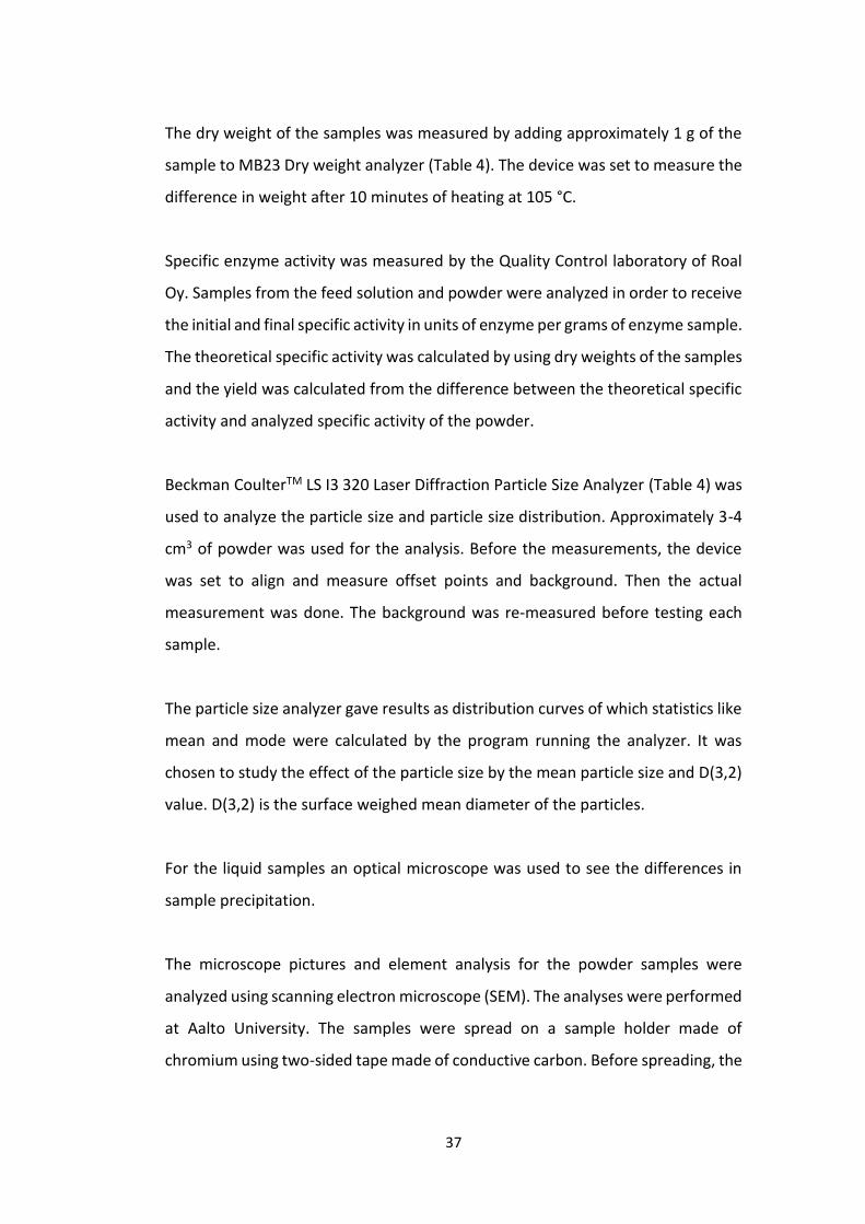
The dry weight of the samples was measured by adding approximately 1 g of the

sample to MB23 Dry weight analyzer (Table 4). The device was set to measure the

difference in weight after 10 minutes of heating at 105 °C.

Specific enzyme activity was measured by the Quality Control laboratory of Roal

Oy. Samples from the feed solution and powder were analyzed in order to receive

the initial and final specific activity in units of enzyme per grams of enzyme sample.

The theoretical specific activity was calculated by using dry weights of the samples

and the yield was calculated from the difference between the theoretical specific

activity and analyzed specific activity of the powder.

Beckman CoulterTM LS I3 320 Laser Diffraction Particle Size Analyzer (Table 4) was

used to analyze the particle size and particle size distribution. Approximately 3-4

cm3 of powder was used for the analysis. Before the measurements, the device

was set to align and measure offset points and background. Then the actual

measurement was done. The background was re-measured before testing each

sample.

The particle size analyzer gave results as distribution curves of which statistics like

mean and mode were calculated by the program running the analyzer. It was

chosen to study the effect of the particle size by the mean particle size and D(3,2)

value. D(3,2) is the surface weighed mean diameter of the particles.

For the liquid samples an optical microscope was used to see the differences in

sample precipitation.

The microscope pictures and element analysis for the powder samples were

analyzed using scanning electron microscope (SEM). The analyses were performed

at Aalto University. The samples were spread on a sample holder made of

chromium using two-sided tape made of conductive carbon. Before spreading, the

38

samples were homogenized by mixing. Light pressure was applied to ensure

adhesion. Then chromium was deposited in 15 nm layers to achieve the required

surface conductivity.

The element analysis was performed along with SEM using energy-dispersive X-

ray spectroscopy (EDS). It is based on the backscattered electrons and

characteristic x-rays from SEM. At least three points were selected for the analysis

in order to determine if there were different types of particles. An element

spectrum and a report were obtained. The analysis could not separate small

elements like hydrogen, carbon, nitrogen and oxygen, but sulphur, phosphorus,

potassium, calcium, sodium and chloride could all be detected.

Statistical analysis for the sample included t-test that was used in hypothesis

testing. Correlation coefficients were calculated to factors that seemed to have

linear correlations. However, there was not parallel samples or repeated

experiments, and thus only several conclusions were statistically relevant.

39

7 Results

In this chapter the results are presented.

7.1 Enzyme 1A

Samples of enzyme 1A were dried without any additives in order to determine the

effect of different cyclones and nozzle caps. The aim was to find the combination

that gives largest particles. The experiment design can be found from Table 7. The

samples named in this work were in the form of JR-X-Y where X represents the

experiments design number (not the perform order) and Y is a running number.

Table 7. Experimental design in order to select cyclone type and nozzle size.

Nozzle cap size (μm)

Cyclone size 140 150

Small JR-2-4 JR-2-3

Large JR-2-2 JR-2-1

The results are divided into four sections. First section shows the results from

particle size distribution analysis, second from SEM, third from elemental analysis

and fourth from specific activity analysis.

7.1.1 Particle size distribution

The particle size distribution was analyzed for all the samples and size distribution

curves were compared. The results can be found in Figure 6, and they suggest that

the large cyclone with 150 μm nozzle cap gives the largest particles. The rest of

the experiments were performed with those settings.

Another interesting result can be found in Figure 6. The scale of spray drying has

an effect on particle size distribution. The same enzyme solution as was spray

dried in the laboratory scale BÜCHI Mini Spray Dryer (Table 4) was spray dried in

40

production scale, and the resulting powders were significantly different. The mean

particle sizes were 14 and 96 μm, respectively.

41

Figure 6. Particle size distribution curves for Enzyme 1A when studying the effect of the cyclone and nozzle cap size suggest that large

cyclone with 150 μm nozzle cap gives the largest particles. The sample dried in production scale differed significantly in terms of particle

size from the other samples.

42

7.1.2 Scanning electron microscope (SEM)

SEM pictures were taken to confirm the results gained from particle size

distribution analysis. In Figure 7 the SEM pictures of samples JR-2-1 (large cyclone,

150 μm nozzle cap), JR-2-2 (large cyclone, 140 μm nozzle cap), JR-2-3 (small

cyclone, 150 μm nozzle cap) and JR-2-4 (small cyclone, 140 μm nozzle cap) are

shown at 1000x magnification. It is clear that the particles are generally larger in

picture A) and smaller in B) and D). Therefore, also SEM pictures support the use

of large cyclone and 150 μm nozzle cap, and corresponds with the particle size

distribution measurements.

Figure 7. SEM pictures of samples of enzyme 1A were taken at 1000x magnification

in order to compare the particle sizes. As can be seen the particles in picture A) are

the largest but there are several larger ones also in C) suggesting that a larger

nozzle cap helps to increase the particle size. A) JR-2-1 B) JR-2-2 C) JR-2-3 D) JR-2-

4.

43

A SEM picture was taken of production scale dried sample of enzyme 1A to

compare it with laboratory scale samples. A 1000x magnification of the particles

(Figure 8) look very different compared to the particles in Figure 7. Remains of

crumpled spheres can be found, but otherwise it would be hard to say that it is the

same material. So, there are remarkable differences between different scales even

in drying the same enzyme solutions, as was also concluded in Section 0.

Figure 8. The particles in SEM picture with 1000x magnification of sample Enzyme

1A from production scale spray dryer (JR-2-5) looks significantly different

compared to laboratory scale and it is strongly agglomerated.

7.1.3 Elemental analysis

Elemental analysis was performed on samples JR-2-2 (large cyclone, 140 μm nozzle

cap) and JR-2-5 (dried in production scale). The analysis could only find larger

molecules like sulphur, potassium and phosphorus. The relative errors in the

measurements were too high to make reliable conclusions on the results. Element

spectrums, data and graphs can be found from Appendix 2.

7.1.4 Specific enzyme activity yield

Specific enzyme activity yields were calculated as enzymes are produced for their

activity. Even if the resulting enzyme powder had a large particle size, if the

enzyme activity was lost the method cannot be considered as effective.

44

Enzyme activity analysis gave the specific activity yields from the drying (Table 8).

There was a drop of around 10 % in the yields for all the samples, which is still at

the acceptable level. The specific activity yield should be 90 % or higher.

Table 8. Specific enzyme activity yields for the samples of enzyme 1A.

Nozzle cap

Cyclone 140 150

Small

Large

92.4 %

88.4 %

88.5 %

90.1 %

7.2 Enzyme 1B

The enzyme solutions of 1B were dried with NaCl and Na2SO4. The concentration

of the enzyme solution was varied by using filtrate, a mixture of filtrate and

concentrate (ratio 1:1) or concentrate in order to see the effect of increased dry

weight. NaCl concentration was 6.8 w/w % and it was blended with enzyme

solutions of different concentrations to see the effect of the enzyme : additive

ratio. Na2SO4 concentrations were 4, 5, 6 and 6.8 w/w % to compare the effect of

NaCl and Na2SO4 and to optimize Na2SO4 concentration.

Samples for enzyme 1B experiments were prepared according to Table 9.

45

Table 9. Experiments for enzyme 1B were done with NaCl and Na2SO4 as additives

and using different enzyme solution and additive concentrations. An additional

sample, JR-1-7, was prepared in similar fashion as JR-1-6 but with 1.5 % of methyl

cellulose.

NaCl concentration Na2SO4 concentration

Enzyme solution 0.0 % 6.8 % 6.80 % 6.0 % 5.0 % 4.0 %

Filtrate JR-1-1 JR-1-4 JR-3-1

Mix JR-1-2 JR-1-5 JR-3-2

Concentrate JR-1-3 JR-1-6 JR-3-3 JR-4-1 JR-4-2 JR-4-3

7.2.1 Particle size distribution

The particle sizes were analyzed by using mean particle sizes and D(3,2) values

(details in Section 6.3.3). Most of the samples show clear trends in mean particle

size but not with D(3,2) (Figure 9). D(3,2) is dependent on the surface and volume

ratio, which might vary if the particles combine into large agglomerates or shrink

to have large surface are but small volume.

Particle size analysis suggested that the increased protein concentration increases

the mean particle size (Figure 9). The effect was greater if additives were included

and the addition of Na2SO4 gave larger particles than NaCl. Use of methyl cellulose

together with NaCl further increased the particle size. The particle size distribution

curves for the samples are shown in Appendix 1.

46

Figure 9. The mean particle size increased when the protein concentration was raised. Without additives (JR-1-1 to JR-1-3) the effect was

small compared to samples with Na2SO4 (JR-3-1 to JR-3-3) and NaCl (JR-1-4 to JR-1-6). Methyl cellulose (JR-1-7) further increased the particle

size of JR-1-6. The sample JR-4-2 seems like it does not fit as the particle size increases from 4.0 to 6.0 and 6.8 w/w % (JR-4-1, JR-4-3 and JR-

3-3, respectively).

0

5

10

15

20

JR-1-1 JR-1-2 JR-1-3 JR-4-3 JR-4-2 JR-4-1 JR-3-1 JR-3-2 JR-3-3 JR-1-4 JR-1-5 JR-1-6 JR-1-7

No No No No No No Yes

0.00 4.00 5.00 6.00 6.80 0.00

0.00 6.80

AHO

Dia

me

ter

(µm

)

Average of PS mean

Average of PS D(3,2)

Mean particle size

D(3,2) of particle size

Methyl cellulose

Na2SO4 concentration (w/w %)

NaCl concentration (w/w %)

47

7.2.2 Scanning electron microscope (SEM)

SEM pictures were taken to confirm the results of particle size analysis and to see

the morphology of the particles. Pictures were only taken of samples with varying

enzyme concentration with or without 6.8 w/w % of NaCl added. In Figure 10, it

can be seen that the number of larger particles increased when the enzyme

concentration increases.

Figure 10. SEM pictures at 1000x magnification of enzyme 1B powders showed

differences in average particle size between the samples with no additives. A) JR-

1-1 (Concentration factor 1) B) JR-1-2 (Conc. factor 1.5) C) JR-1-3 (Conc. factor 2)

Figure 11. A) SEM pictures at 1000x magnification reveal that increased enzyme

concentration with NaCl increase the mean particle size. JR-1-4 (6.8 w/w % NaCl,

Conc. factor 1) B) JR-1-5 (6.8 w/w % NaCl, Conc. factor 1.5) C) JR-1-6 (6.8 w/w %

NaCl, Conc. factor 2)

Furthermore, the morphology of the particles with NaCl is different. While the

particles without NaCl look the same even though the size varies, the small

particles with NaCl look different than larger particles. Also, the 2500x

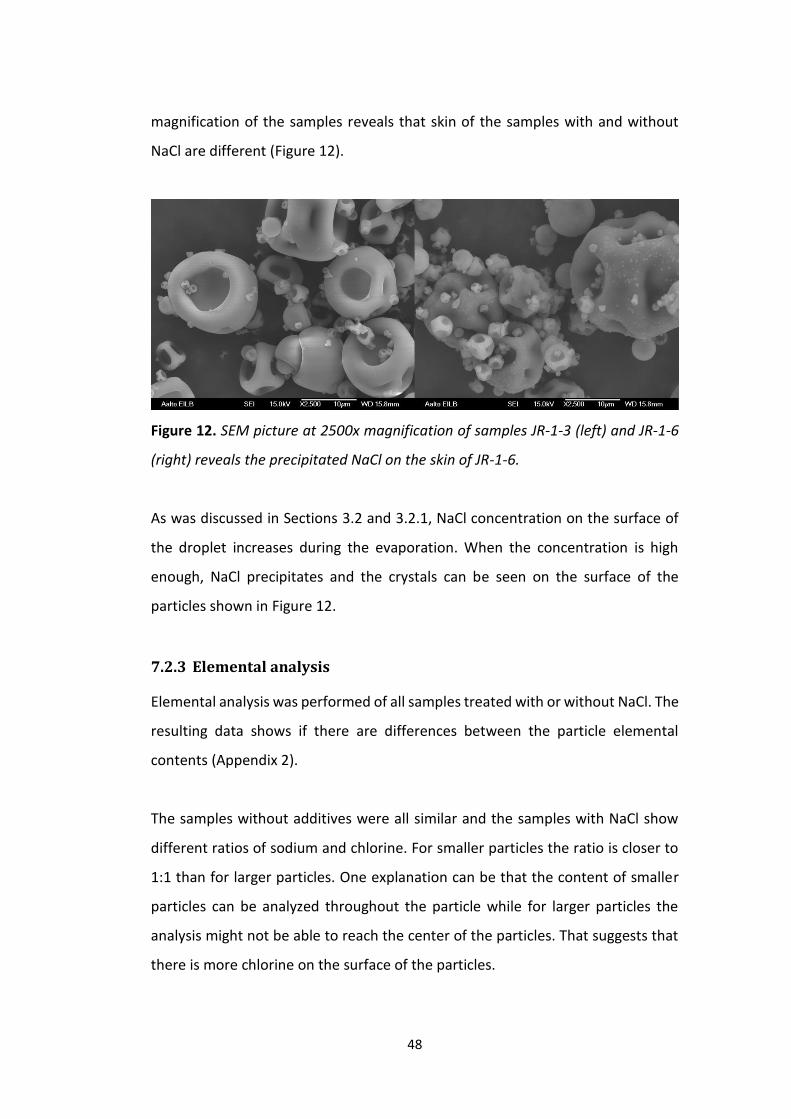
48

magnification of the samples reveals that skin of the samples with and without

NaCl are different (Figure 12).

Figure 12. SEM picture at 2500x magnification of samples JR-1-3 (left) and JR-1-6

(right) reveals the precipitated NaCl on the skin of JR-1-6.

As was discussed in Sections 3.2 and 3.2.1, NaCl concentration on the surface of

the droplet increases during the evaporation. When the concentration is high

enough, NaCl precipitates and the crystals can be seen on the surface of the

particles shown in Figure 12.

7.2.3 Elemental analysis

Elemental analysis was performed of all samples treated with or without NaCl. The

resulting data shows if there are differences between the particle elemental

contents (Appendix 2).

The samples without additives were all similar and the samples with NaCl show

different ratios of sodium and chlorine. For smaller particles the ratio is closer to

1:1 than for larger particles. One explanation can be that the content of smaller

particles can be analyzed throughout the particle while for larger particles the

analysis might not be able to reach the center of the particles. That suggests that

there is more chlorine on the surface of the particles.

49

7.2.4 Specific activity yield

Specific activity yield was calculated to ensure no activity was lost due to use of

additives. The results of the analysis (Appendix 3) showed high errors and some

results were omitted. In general it seemed like the use of NaCl increased the

activity yield compared to samples without additives. Methyl cellulose did not

have the same effect.

For Na2SO4 treated samples it was not possible to make any conclusions about

activity yields. The analysis should be repeated or another analysis method

considered. One reason for the problems in the analysis was that it was designed

for another similar enzyme.

7.3 Enzyme 2

The experiments for enzyme 2 were designed so that the effects could be

compared with the effects seen with enzymes 1B and 3. The experimental design

is represented in Table 10.

Table 10. The experiments for enzyme 2 concentrated on studying the effect of

NaCl concentration and pH. Also Na2SO4 and methyl cellulose (MC) were tested.

Concentration (w/w %) NaCl Na2SO4

6.8

JR-6-1

12.5

JR-6-4

JR-6-5

15

JR-6-6

JR-6-7

6.8

JR-6-3

pH 4.8 (=no pH control)

pH 8

1.5 % MC JR-6-2

7.3.1 Particle size distribution

Particle size of the samples was measured and the results are summarized in Table

13 showing the mean particle sizes and d(3,2) values. It can be seen that the use

of Na2SO4 increased the particle size compared to samples treated with NaCl.

50

Additionally, methyl cellulose increased the particle size when used together with

NaCl. When NaCl concentration is increased the effect of NaCl stayed similar but

the effect of pH was stronger. For enzyme 2, the pH 4.8 seemed to be more

optimal than pH 8.

The particle size distribution curves received from the analysis are represented in

Appendix 1.

Figure 13. The effect of Na2SO4 on particle size of enzyme 2 is stronger than that

of NaCl. However, methyl cellulose together with NaCl increased the particle size

compared to sample without methyl cellulose. Also pH has an effect as pH 4.8

seems to be more optimal than pH 8.

7.3.2 Specific enzyme activity yield

Table 11 shows the specific activity yields calculated from the specific activity

measurements. Most of the yields were over 100 % suggesting that there was

some error in the measurements, even though enzyme 2 was known to be stable

and high specific activity yields were expected.

0

5

10

15

20

JR-6-3 JR-6-1 JR-6-2 JR-6-4 JR-6-5 JR-6-6 JR-6-7

No No Yes No No No No

4.80 4.80 4.80 8.00 4.80 8.00

6.80 0.00 0.00 0.00

0.00 6.80 12.50 15.00

AFK

Dia

me

ter

(µm

)

Average of PS mean

Average of PS D(3,2)

Mean particle size

Particle size D(3,2)

Methyl cellulose

pH

Na2SO4 conc. (w/w %)

NaCl conc. (w/w %)

51

Table 11. Specific activity yields of enzyme 2 were mostly above 100 % suggesting

problems in the analysis. However, it seems like the additives did not lower the

activity yield of the enzyme.

Concentration (w/w %) NaCl Na2SO4

6.8

99.6 %

12.5

103.7 %

112.7 %

15

100.7 %

106.2 %

6.8

-

pH 4.8 (=no pH control)

pH 8

MC 107.2 %

7.4 Enzyme 3

The experiments were performed with enzyme solutions from production and two

different pilot scale fermentations named as enzymes 3.1, 3.2 and 3.3. Enzymes

3.1 and 3.2 were similar production processes performed at different scales.

Enzyme 3.3 was produced at pilot scale but in differing media. The enzyme

produced in each of the scales was the same enzyme and produced by the same

strain. The experimental designs are represented in Tables 12‒14.

Table 12. Experiments with enzyme 3.1 Sample JR-5-21 (15 % NaCl + 2 % Ca-

acetate + 1.5 % methyl cellulose) is missing from the table.

NaCl NaCl + 2 % Ca-Ac

NaCl concentration (w/w %)

pH 5 (=no pH control)

pH 8 pH 9 pH 4.5 pH 5,5

(=no pH control)

pH 8

0 JR-5-1 JR-5-6 JR-5-10

5 Jr-5-2 JR-5-7 JR-5-11

7.5 JR-5-3 JR-5-8 JR-5-12

12.5 JR-5-4 JR-5-5 JR-5-15 JR-5-9 JR-5-13 JR-5-14

15 JR-5-16 JR-5-17 JR-5-18 JR-5-19 JR-5-20

52

Table 13. The experimental design for enzyme 3.2.

Concentrate FIltrate

Only NaCl NaCl + 2 % Ca-Ac NaCl + 2 % CaCl2 Only

NaCl

NaCl concentration

(w/w %)

pH 5 (=no pH control)

pH 8 pH 6

(=no pH control)

pH 8 pH 5

(=no pH control)

pH 8 pH 5

(=no pH control)

5

7.5

12.5

15

17.5

20

JR-5-35

JR-5-36

JR-5-37

JR-5-38

JR-5-39

JR-5-40

JR-5-41

JR-5-43

JR-5-44

JR-5-46

JR-5-47

JR-5-48

JR-5-49

53

Table 14. The experimental design for enzyme 3.3.

Concentrate Filtrate

Only NaCl NaCl + 2

% Ca-Ac

NaCl + 0.5 % ascorbic

acid Only NaCl

NaCl

concentration

(w/w %)

pH 5 (=no

pH control) pH 8 pH 8.5 pH 8

pH 5 (=no

pH control) pH 8

pH 5 (=no

pH control) pH 8 pH 8.5

5

12.5

15

17.5

20

JR-5-50

JR-5-52

JR-5-51

JR-5-53

JR-5-54

JR-5-55

JR-5-56

JR-5-57

JR-5-59

JR-5-58

JR-5-60

JR-5-61

JR-5-62

JR-5-64

JR-5-65

JR-5-66

JR-5-63

54

7.4.1 Particle size distribution

The largest particles of all the three groups of experiments were received from

production material (enzyme 3.1). Samples with NaCl concentration of 12.5 or 15

% and no Ca-acetate gave the largest mean particle size of around 200 µm (Figure

14). The largest particles had the diameter of 1000 µm (Appendix 1, Figure 6).

Figure 14. Particle size was measured for all the powder samples of enzyme 3.1

and it can clearly be noticed that samples JR-5-4 (12.5 % NaCl, no pH control), JR-

5-5 (12.5 % NaCl, pH 8), JR-5-15 (12.5 % NaCl, pH 9), JR-5-16 (15 % NaCl, no pH

control) and JR-5-17 (15 % NaCl, pH 8) had larger particle size than other samples.

Spray drying of the enzyme solution without additives was impossible as no

powder was produced, and thus they are missing from Figure 14. Also the sample

with methyl cellulose could not be spray dried.

0

50

100

150

200

250

JR-5

-2

JR-5

-11

JR-5

-8

JR-5

-3

JR-5

-12

JR-5

-9

JR-5

-4

JR-5

-13

JR-5

-5

JR-5

-14

JR-5

-15

JR-5

-18

JR-5

-16

JR-5

-19

JR-5

-17

JR-5

-20

No Yes Yes No Yes Yes No Yes No Yes No Yes No Yes No Yes

5.00 4.50 5.00 4.50 5.00 8.00 9.00 4.50 5.00 8.00

5.00 7.50 12.50 15.00

Production1

Dia

me

ter

(µm

)

Average of PS mean

Average of PS D(3,2)

Mean particle size

Particle size D(3,2)

pH

NaCl conc. (w/w %)

Ca-acetate

55

Figure 15 reveals that the particle size of powder samples of enzyme 3.2 were over

10 times smaller than of enzyme 3.1. However, also here the NaCl concentrations

12.5 and 15 % without Ca-acetate or CaCl2 gave the largest particles.

Figure 15. The addition of 12.5 or 15 % of NaCl and not using Ca-acetate or CaCl2

resulted the largest mean particle sizes for the powder of enzyme 3.2.

Figure 15 also shows that with 12.5 % NaCl filtrate could be spray dried and large

particles received, which would be beneficial in the industries where

concentration of the solutions take a long time.

The mean particle size of powders of enzyme 3.3 was not strongly affected by

additives (Figure 16). The use of Ca-acetate reduced the particle size as in the

previous experiments. The use of ascorbic acid did not increase the particle size.

0

5

10

15

20

JR-5

-35

JR-5

-36

JR-5

-39

JR-5

-37

JR-5

-46

JR-5

-43

JR-5

-40

JR-5

-38

JR-5

-44

JR-5

-41

JR-5

-47

JR-5

-48

JR-5

-49

Conc. Conc. Conc. Conc. Filtrate Conc. Conc. Conc. Conc. Conc. FiltrateFiltrateFiltrate

No No No No Yes No No Yes No No No No

No No Yes No Yes No Yes No No No

5.00 5.00 6.00 5.00 6.00 8.00 5.00 5.00 5.00

5.00 7.50 12.50 15.00 17.50 20.00

Dia

me

ter

(µm

)

Average of PSmean

Average of PSD(3,2)

Mean

particle size

Particle size

D(3,2)

CaCl2

Ca-acetate

pH

NaCl conc. (w/w %)

56

A new type of problem was discovered with the enzyme 3.3 The samples JR-5-53

(12.5 % NaCl, pH 8), JR-5-54 (12.5 % NaCl, pH 8.5) and JR-5-55 (5 % NaCl + 2 % Ca-

acetate, pH 8), which had pH adjusted, turned into gels that could not be spray

dried. Also other samples from concentrate had a gel-like structure, but the ones

with ascorbic acid did not have that problem.

Figure 16. The mean particle size of samples of enzyme 3.3 was not affected by

additives strongly. The addition of Ca-acetate reduced the particle size as was

expected. The use of ascorbic acid did not increase the particle size.

When the results of the three experiments are combined it can be concluded that

the additives can be used to change the mean particle size, but that there is an

unknown factor that affects the strength of the effect.

For example, the effect of pH can be seen most clearly with enzyme 3.1. Different

pH is optimal at different NaCl concentration as can be noticed from Figure 14. For

0

5

10

15

20

JR-5

-50

JR-5

-57

JR-5

-51

JR-5

-58

JR-5

-52

JR-5

-61

JR-5

-59

JR-5

-62

JR-5

-60

JR-5

-56

JR-5

-63

JR-5

-64

JR-5

-65

JR-5

-66

Conc. Conc. Conc. Conc. Conc. Filt. Conc. Filt. Conc. Conc. Filt. Filt. Filt. Filt.

No Yes No Yes No Yes No Yes No No No No No

No No No No Yes No No No No

4.50 8.00 4.50 8.00 8.50 8.00 8.00 8.00

5.00 12.50 15.00 17.50 20.00

Pilot2

Dia

me

ter

(µm

)

Average of PSmean

Average of PSD(3,2)

Mean particle size

Particle size D(3,2)

Ascorbic acid

Ca-acetate

pH

NaCl conc. (w/w %)

57

enzyme 3.1, the optimal pH for higher particle size was at pH 8–9 at 12.5 w/w %

NaCl concentration while at 15 w/w % it was pH 5. Thus, we can determine that

pH affects particle size, but the effect is not independent of other known factors.

Also, the same effects seen with enzyme 3.1 could not be seen with enzymes 3.2

and 3.3. The explanation could not be found, and thus more studies on the

differences between these materials should be performed.

Particle size distribution curves can be found from Appendix 1. The most

interesting result seen in the curves was that the samples with largest particle sizes

lacked the smallest particles in the distribution curves. Those were the samples of

enzyme 3.1 and using the same conditions for the enzymes 3.2 and 3.3, the same

effect was not seen. One goal of this work was to find a method to remove the

smallest particles. However, the factors that caused that are still unknown.

7.4.2 Scanning electron microscope (SEM)

SEM pictures were taken to confirm the results of particle size distribution

analysis. The pictures of the samples with the largest mean particle size revealed

that the particle size itself did not increase as much as was expected. Instead, the

mean particle size was increased mostly by agglomeration, where agglomerates

consisted of particles of around 10 µm in diameter.

However, the increased number of large particles also helped to increase the

mean particle size. SEM pictures of samples of enzyme 3.1 with the largest mean

particle size are represented in Figure 17.

58

Figure 17. SEM pictures at 1000x magnification reveal the reason why samples JR-

5-5 (B) and JR-5-16 (D) give larger mean particle size from the particle size analysis.

Comparing them with JR-5-4 (A), JR-5-15 (C) and JR-5-17 (E) the clear difference in

agglomeration can be seen.

Agglomeration was also a reason why several samples of enzyme 3.2 had larger

particles, while samples of enzyme 3.3 did not. As can be seen in the left panel of

Figure 18, smaller particles are connected to larger particles, whereas in the right

panel this was not observed as strongly.

59

Figure 18. SEM pictures of samples from Pilot 1 (JR-5-37, left) and Pilot 2 (JR-5-52,

right) at 1000x magnification showed different amounts of sample agglomeration,

even though the particles are approximately the same size. This leads to greater

mean particle size in particle size analysis.

Particles with different additive concentrations looked different. Lower NaCl

concentration led to “crumbled” particles whereas higher salt concentration to

smoother spheres. This seems to apply to both scales and if another additive was

used along with NaCl. In Figure 19, samples of enzymes 3.1 and 3.3 with 5 and 12.5

% of NaCl were compared. Samples of enzyme 3.3 also contained 0.5 % of ascorbic

acid, as the samples without it could not be dried.

60

Figure 19. SEM pictures from samples A) JR-5-2 (5 w/w % NaCl, Production 1) B)

JR-5-4 (12.5 w/w %, Production 1) C) JR-5-57 (5 w/w % NaCl + 0.5 w/w % ascorbic

acid, Pilot 2) and D) JR-5-59 (12.5 w/w % NaCl + 0.5 w/w % ascorbic acid, Pilot 2)

were taken at magnification 2500x. They show how the lower NaCl concentration

causes particles to look more “crumpled” compared to higher NaCl containing

particles. Also, it can be seen in picture D) that particles seem to be hollow.

To give a reference to particles with small mean particle sizes and highlight the

importance of agglomeration, samples JR-5-5 (12.5 % NaCl, pH 8) and JR-5-14 (12.5

% NaCl + 2 % Ca-acetate, pH 8) of enzyme 3.1 are represented in Figure 20.

61

Figure 20. 2500x magnification SEM pictures of samples JR-5-5 (12.5 % NaCl, pH 8)

and JR-5-14 (12.5 % NaCl + 2 % Ca-acetate, pH 8) from Production 1 show the

importance of agglomeration in reduction of individual small particles.

7.4.3 Element analysis

Elemental analysis was performed to samples several samples and the samples

were chosen according to results of the particle size distribution analysis as well

as due to interest in production applications. However, the received information

only confirmed the presence of calcium in the samples.

The reason why the experiment was not as informative as expected was that the

elemental composition was only fully analyzable for small particles. The aim of this

analysis was to see the differences in particles with different morphologies but

that was not possible. The elemental analysis results are represented in Appendix

2.

7.4.4 Specific enzyme activity yield

The specific enzyme activity yields were calculated for drying process and the

graphs are represented in Figures 21‒23. The acceptable loss was around 10 % to

consider the usage of the method in possible future applications.

62

Samples with NaCl concentration between 5 and 12.5 % do not show significant

activity losses. Ca-acetate lowers the specific activity yield of enzyme 3.1 but not

of enzymes 3.2 and 3.3. Also extreme pH 9 causes specific enzyme activity loss.

For enzymes 3.2 and 3.3 CaCl2 significantly lowers the yield as well spray drying of

filtrate samples. Therefore, the promising results gained from the increased mean

particle size with filtrate samples cannot be considered as an effective method.

63

Figure 21. Specific activity yields of enzyme 3.1 were above 90 % for samples with NaCl concentration between 5 and 12.5 % without Ca-

acetate. The samples with Ca-acetate had only several samples with specific activity yields over 90 %. The samples without NaCl and with

methyl cellulose could not be spray dried.

50

60

70

80

90

100

JR-5

-1

JR-5

-2

JR-5

-3

JR-5

-4

JR-5

-5

JR-5

-15

JR-5

-16

JR-5

-17

JR-5

-6

JR-5

-10

JR-5

-7

JR-5

-11

JR-5

-8

JR-5

-12

JR-5

-9

JR-5

-13

JR-5

-14

JR-5

-18

JR-5

-21

JR-5

-19

JR-5

-20

No No No No No No No No No No No No No No No No No No Yes No No

5.00 5.00 5.00 5.00 8.00 9.00 5.00 8.00 4.50 5.00 4.50 5.00 4.50 5.00 4.50 5.00 8.00 4.50 5.00 8.00

0.00 5.00 7.50 12.50 15.00 0.00 5.00 7.50 12.50 15.00

No Yes

Production1

Spe

cifi

c ac

tivi

ty y

ield

(%

)

Methyl cellulose

pH

NaCl conc. (w/w %)

Ca-acetate

64

Figure 22. Specific activity yields of enzyme 3.2 varied significantly. CaCl2 lowered

the yield more than Ca-acetate. All the samples with NaCl and with or without Ca-

acetate had a specific activity yield over 90 %. Samples from filtrate had high

activity loss.

60

80

100

120

JR-5

-35

JR-5

-36

JR-5

-37

JR-5

-38

JR-5

-43

JR-5

-44

JR-5

-39

JR-5

-40

JR-5

-41

JR-5

-46

JR-5

-47

JR-5

-48

JR-5

-49

5.00 5.00 5.00 8.00 5.00 8.00 6.00 6.00 8.00 5.00 5.00 5.00 5.00

5.00 7.50 12.50 12.50 7.50 12.50 12.50 15.00 17.50 20.00

No Yes No No

No Yes No

Conc. Filt.

Spe

cifi

c av

tivi

ty y

ield

(%

)

pH

NaCl conc. (w/w %)

CaCl2

Ca-acetate

65

Figure 23. Specific activities of enzyme 3.3 show that the activity yields from filtrate

samples were significantly low. Also it can be noticed that the samples with

ascorbic acid had slightly smaller activity yields compared to samples without.

7.5 Material balance

Material balances were calculated for all the spray dried samples. By weighing, the

feed mass and the produced powder mass could be measured. After measuring

the dry weight of the feed solution and the powder, the material loss could be

calculated.

The material balance can be written in the form of Equation 30.

𝐴𝐶𝐶 = 𝐼𝑁 − 𝑂𝑈𝑇 (30)

Figure 24 shows the chart on spray drying with BÜCHI Mini Spray Dryer B-290.

60

80

100

120

JR-5

-50

JR-5

-57

JR-5

-51

JR-5

-58

JR-5

-52

JR-5

-59

JR-5

-60

JR-5

-56

JR-5

-61

JR-5

-62

JR-5

-63

JR-5

-64

JR-5

-65

JR-5

-66

No Yes No Yes No Yes Yes No No No No No No No

No No No No Yes No No No No No No

4.50 8.00 4.50 8.00 4.50 8.00 8.50 8.00 8.00 8.00

5.00 12.50 12.50 15.00 17.50 20.00

Conc. Filt.

Pilot2

Spe

cifi

c ac

tivi

ty y

ield

(%

)

Ascorbic acid

Ca-acetate

pH

NaCl conc. (w/w %)

66

Figure 24. Chart to describe the material balance of spray drying with BÜCHI Mini

Spray Dryer B-290.

The material loss was calculated using Equation 31.

𝑀𝑎𝑡𝑒𝑟𝑖𝑎𝑙 𝑙𝑜𝑠𝑠 (%)

=𝑝𝑜𝑤𝑑𝑒𝑟 𝑜𝑢𝑡 (𝑔) × 𝑝𝑜𝑤𝑑𝑒𝑟 𝑑𝑟𝑦 𝑚𝑎𝑠𝑠 (%)

𝑓𝑒𝑒𝑑 𝑖𝑛 (𝑔) × 𝑓𝑒𝑒𝑑 𝑑𝑟𝑦 𝑚𝑎𝑠𝑠 (%)

× 100 %

(31)

Material losses varied from sample to sample between values 5-100 %. However,

the mean material loss was 32 % (median 29 %). The lowest material losses were

received with the high performance cyclone and the highest losses with enzyme 3

samples without additives. Enzyme 1B had the highest mean material loss (36 %)

and enzyme 1A the lowest (20 %). Enzymes 2 and 3 had mean material losses of

23 and 34 %, respectively.

The material losses obtained using BÜCHI Mini Spray Dryer B-290 do not correlate

with losses of the spray dryer used in the production. The material losses in

laboratory scale are generally higher, and in this study material losses were

studied to see if sample treatment affected the lost materials. However,

connection between material losses and mean particle sizes could not be found.

67

7.6 Statistical analysis

Statistical analysis was used in hypothesis testing to show the differences between

samples and to prove that the results were statistically relevant. Also the

correlations between parameters were studied. Statistical analysis methods were

described in detail in Chapter 4.

7.6.1 Effect of calcium on particle size in Enzyme 3

Hypothesis testing was used to study the effect of calcium on particle size of

Enzyme 3. The mean particle size analyzed by the particle size analyzer was used

as a test parameter.

The hypothesis was tested by t-test for two random variables with different

variances (Section 4.2).

Hypothesis was that “Ca-acetate increases the particle size”, and the null

hypothesis H0 was defined as

H0 ∶ Pno Ca−Ac = PCa−Ac (32)

where P refers to mean particle size. Alternative hypotheses were

H1 ∶ Pno Ca < PCa (33)

H1 ∶ Pno Ca > PCa (34)

The filtrate samples are no included in the analysis as there were not filtrate

samples including calcium. t-value was calculated to be 20.7 and t0.05 = 1.796 (df =

11). Thus the hypothesis is rejected and the alternative hypothesis Pno Ca < PCa

applies. Mean, variance and the number of samples are collected to Table 15.

68

Table 15. Arithmetic mean, variance and the number of samples that were used to

calculate t-value for the data of specific activity yield for Enzyme 3. Samples from

filtrate were not included.

Arithmetic mean Variance Number of

samples

No calcium 59.2 65.4 12

Calcium 10.3 2.1 15

7.6.2 Effect of calcium acetate on specific activity yield in enzyme 3

The effect of calcium acetate on specific activity yield was studied for enzyme 3.1

data. The result can be seen from the graphs but using hypothesis testing, the

statistical reliability can be ensured.

The original hypothesis was that Ca-acetate stabilizes the protein structure and

therefore increases the specific activity yield. That hypothesis was tested by t-test

for two random variables with different variances (Section 4.2).

Hypothesis was that “Ca-acetate increases the specific activity yield”, but the null

hypothesis H0 was defined as

H0 ∶ Ano Ca−Ac = ACa−Ac (35)

where A refers to specific activity yield. Alternative hypotheses were

H1 ∶ Ano Ca−Ac < ACa−Ac (36)

H1 ∶ Ano Ca−Ac > ACa−Ac (37)

The arithmetic mean, variance and the number of samples of the enzyme 3.1 data

are compiled in Table 16. By using Equation 13 the t-value was calculated for the

data, and the resulting t-value was 2.073. Equation 16 was used to calculate the

69

degree of freedom (df = 11) and the significance level of 0.05 was chosen.

Statistical tables gave a t0.05-value of 1.796. As the t > t0.05, the null hypothesis was

rejected and alternative hypothesis Ano Ca-Ac > Aca-Ac applied. Therefore, the

conclusion is that calcium acetate does not increase the specific activity yield.

Table 16. Arithmetic mean, variance and the number of samples were used to

calculate t-value for the data of Production 1 of specific activity yield for Enzyme 3.

Arithmetic mean Variance Number of

samples

No calcium 91.7 31.88 7

Calcium 86.3 21.99 10

The hypothesis was tested with all the enzyme 3 samples and without including

filtrate samples. The result with all the samples was that calcium acetate increases

the specific yield activity. One factor affecting to that result was the low activities

gained from filtrate samples and calcium acetate was not added to those. When

filtrate samples were not included, the result was the same as with enzyme 3.1

samples: calcium does not increase the specific activity yield.

7.6.3 Protein concentration correlations

Values of r for linear correlation were calculated for enzyme 1B. The effect of

increased protein concentration on mean particle size was seen in Figure 9

(samples JR-1-3 to JR-1-3) as well as the effect of Na2SO4 and NaCl at different

protein concentrations (JR-3-1 to JR-3-3, and JR-1-4 to JR-1-6, respectively). The

linear correlation lines with the r (R2 in the figure) and the functions are presented

Figure 25.

70

Figure 25. Linear correlation was discovered to samples of enzyme 1B. Increased

protein concentration increases the mean particle size. The effect is stronger when

6.8 w/w % of NaCl is added and further increases when using 6.8 % of Na2SO4.

Linear correlations were 0.939, 0.999 and 0.935, respectively. Therefore, it is

possible to say that there are linear correlations between the protein

concentration and mean particle size. The reasons were described in Section 8.1.

8 Discussion

In this chapter the effect of different additives on enzyme particle size and

differences of enzymes and other affecting factors are discussed and compared

with the results from previous studies.

8.1 NaCl, Na2SO4 and pH

The use of NaCl and Na2SO4 as additives was one way to increase mean particle

size and agglomeration. It was expected that increase in dry weight that can be

y = 0,743x + 8,6717R² = 0,939

0

5

10

15

20

Filtrate Mix Concentrate

Me

an p

arti

cle

siz

e (

µm

)

No additives

y = 2,1695x + 6,9513R² = 0,935

0

5

10

15

20

Filtrate Mix Concentrate

Me

an p

arti

cle

siz

e (

µm

) 6.8 % NaCl

y = 3,467x + 5,7447R² = 0,9999

0

5

10

15

20

Filtrate Mix Concentrate

Me

an p

arti

cle

siz

e (

µm

)

6.8 % Na2SO4

71

performed by adding salt increases the particle size (Table 1) and it was proven by

using different enzyme solution concentrations. This applies with the previous

studies4. However, the gelatinizing effect discovered by Sloth et al. was not seen

in this study even at high concentrations22.

However, another interesting phenomenon was discovered. NaCl and Na2SO4

precipitated proteins in the feed solution and increased the mean particle size and

agglomeration. Precipitation of proteins is known to be used in spray drying to

increase stability of sensitive products20 but its effect on particle size has not been

studied before.

Na2SO4 precipitated proteins more effectively than NaCl and caused more

precipitate in the feed solution. The mean particle size of samples with Na2SO4 was

also greater than with NaCl (Figure 9 and Figure 13). According to Hofmeister

series, sulphate has higher ability to precipitate proteins than chloride54.

Therefore it seems that the mean enzyme particle size can be increased by

choosing a proper salt for enzyme precipitation.

In addition to the use of NaCl and Na2SO4 as additives that precipitated the enzyme

from the solution, also pH caused precipitation. The effect of pH on particle size

have not been studied before but it is known the effect the enzyme precipitation54,

and precipitation of enzyme was discovered to increase the mean particle size and

agglomeration. Though, that should be confirmed by repeating the experiments.

As enzymes are often sensitive and degrade in the presence of high salt

concentrations or extreme pH conditions, it is important to study the specific

activities too. For instance, filtrate samples the solution dry weight was so low that

it was necessary to add high concentrations of NaCl in order to spray dry the

sample. However, that caused high losses in specific enzyme activity yields and

therefore cannot be considered as an effective method.

72

The varying ability of enzyme to precipitate could possibly explain the differences

between enzymes 1B, 2 and 3. Enzyme 3 precipitated easier than 1B while enzyme

2 hardly formed any precipitate at all. Also there were differences between the

enzyme 3.1, 3.2 and 3.3 abilities to precipitate. Thus, further studies on enzyme

precipitation could help to increase the particle size and confirm the connection

between the particle size and ability of an enzyme to precipitate.

8.2 Methyl cellulose

The use of methyl cellulose as an additive in spray drying of enzymes was studied

with enzymes 1B, 2 and 3.

In the case of enzyme 1B, high amount of powder was stuck in the bottom of the

drying chamber when methyl cellulose was used (Figure 26). This suggests that the

powder was too heavy for the underpressure to transfer it to cyclone. Particles

can be heavy due to moisture remaining in the particles or strong agglomeration.

However, strong agglomeration was not seen in SEM pictures.

In the case of enzyme 2, the use of methyl cellulose increased the mean particle

size. However, the number of small particles in particle size analysis was not

significantly affected.

Methyl cellulose was also added to Enzyme 3.1 with 12.5 w/w % NaCl and 2.0 w/w

% of Ca-acetate. As a result the nozzle was blocked and none of the solution could

be dried. That is an interesting effect as in the previous studies methyl cellulose

was used to help to spray dry sticky or caking products.

73

Figure 26. High amounts of enzyme powder (JR-1-7: 6.8 w/w % of NaCl + 1.5 w/w

% methyl cellulose) was stuck in the bottom of the drying chamber due to stickiness

and heaviness. Heavy but dry particles would have been collected into chamber

sample dish.

Methyl cellulose was expected to increase the particle size as it increases the dry

weight. However, it did not increase the agglomeration as expected and therefore

did not reduce the number of small particles. Also it was not expected to be sticky

or cause caking and blocking as it has been used as an additive to reduce stickiness

and caking19.

8.3 Scale and fermentation differences

For enzyme 3, experiments with materials from pilot scale and production scale

were done. There were significant differences in the particle sizes from the

samples of the different experiments. The largest pilot scale samples had over 10

times smaller mean particle size compared to production scale samples.

The samples were prepared similarly and the effect of sample age (difference

between sample preparation and drying dates) and other factors were studied to

find the reason. However, it seems like there is an unknown factor to explain why

the particles of enzyme 3.1 were significantly larger. It would have been

interesting to repeat experiments of enzyme 3.1 with another batch from

74

production. However, the material was not available. Those experiments would

either help to confirm the results gained in this study or increase understanding

of the unknown factor or factors.

For enzyme 1A the scale difference was studied by spray drying the same material

but at different scales. The product from production scale spray dryer was

significantly larger and morphologically different compared to same material dried

with BÜCHI Mini Spray Dryer. There were several reasons for the differences

including differing nozzles and recycling of dust back to drying chamber.

Therefore, it was hard to say if the results gained in laboratory scale with BÜCHI

Mini Spray Dryer apply to production scale. That requires further studies.

The results and discussion above suggest that even small differences in the

material can cause high variation in the end product.

8.4 Reliability

In order to draw reliable conclusions from the results, the experiments should be

repeated. However, it was impossible for this work as the time and availability of

materials were limited and spray drying of samples took time. To confirm the

results and observations of these experiments, the number of samples should be

increased significantly.

Statistically reliable results were only gained of the effects of Ca-acetate, as there

were several samples with Ca-acetate that could be compared and analyzed.

9 Conclusion

In conclusion, the particle size can be affected by additives. Depending on the

enzyme material the optimal additives and their concentrations vary. The most

important discovery in this work was that the ability of the enzyme to precipitate

75

in the sample increased the mean particle size and agglomeration. As

agglomeration is important in reduction of small particles, the additives that favor

agglomeration helped to reduce the number of small particles in enzyme powder.

10 Further studies

Further studies are necessary in order to understand the effects of different

additives better and to optimize the concentrations of additives.

Also, it seems like sodium chloride and sodium sulphate salts precipitate the

proteins but some enzyme samples did not precipitate. The challenge is to find an

additive that increases the agglomeration in those samples that did not

precipitate.

The differences caused by different materials of the same enzyme need more

research as there are still unknown factor or factors affecting the results.

Scale-up might be hard as the laboratory scale spray dryer did not model well with

the production scale spray dryer. Thus, in order to apply the results on larger scale,

further studies with either different laboratory scale or pilot scale spray dryers are

necessary to see if the phenomena discovered in the study apply in other spray

dryers.

76

References

1. Percy S, inventorImprovement in Drying and Concentrating Liquid Substances by

Atomizing. 1872.

2. Masters K. Spray drying handbook. 3rd ed. London: George Godwin Limited; 1979.

3. Keshani S, Daud WRW, Nourouzi MM, Namvar F, Ghasemi M. Spray drying: An

overview on wall deposition, process and modeling. J Food Eng. 2015;146:152-162.

4. Kleinhans S, Arpagaus C, Schrönenberger G, eds. The laboratory assistant. 3rd ed.

Switzerland: Büchi Labortechnik AG; 2007.

5. Okuyama K, Wuled Lenggoro I. Preparation of nanoparticles via spray route. Chemical

Engineering Science. 2003;58(3–6):537-547.

6. Her J, Song C, Lee SJ, Lee K. Preparation of kanamycin powder by an optimized spray

freeze-drying method. Powder Technol. 2010;199(2):159-164.

7. Bandari B, Bansal N, Zhang M, Schuck P, eds. Handbook of food powders - processes

and properties. Elsevier; 2013.

8. Mezhericher M, Levy A, Borde I. Multi-scale multiphase modeling of transport

phenomena in spray-drying processes. Dry Technol. 2015;33(1):2-23.

9. Sloth J. Method for improving spray drying equipment and product properties.

InterCeram. 2010;59(3):193-197.

10. De Jesus SS, Maciel Filho R. Drying of a-amylase by spray drying and freeze-drying - A

comparative study. Brazil J Chem Eng. 2014;31(3):625-631.

77

11. Iskandar F, Gradon L, Okuyama K. Control of the morphology of nanostructured

particles prepared by the spray drying of a nanoparticle sol. J Colloid Interface Sci.

2003;265(2):296-303.

12. Nandiyanto ABD, Hagura N, Iskandar F, Okuyama K. Design of a highly ordered and

uniform porous structure with multisized pores in film and particle forms using a

template-driven self-assembly technique. Acta Materialia. 2010;58(1):282-289.

13. Nandiyanto ABD, Okuyama K. Progress in developing spray-drying methods for the

production of controlled morphology particles: From the nanometer to submicrometer

size ranges. Adv Powder Technol. 2011;22(1):1-19.

14. Mezhericher M, Levy A, Borde I. Modelling the morphological evolution of

nanosuspension droplet in constant-rate drying stage. Chemical Engineering Science.

2011;66(5):884-896.

15. Prinn KB, Constantino HR, Tracy M. Statistical modeling of protein spray drying at the

lab scale. AAPS PharmSciTech. 2002;3(1).

16. Tan LW, Ibrahim MN, Taip FS. Empirical model of spray drying of whole milk powder

using nozzle atomizer spray dryer. J Food Agric Environ. 2010;8(3-4 PART 1):247-252.

17. Muzaffar K, Kumar P. Effect of soya protein isolate as a complementary drying aid of

maltodextrin on spray drying of tamarind pulp. Drying Technology. 2016;34(1):142-148.

18. Ferrari CC, Ribeiro CP, Liserre AM, Moreno I, Marconi Germer SP, De Aguirre JM.

Spray drying of blackberry juice using maltodextrin or gum arabic as carrier agents. Int

78

CIGR Tech Symp - Towards Sustainable Food Chain: Food Process, Bioprocessing Food

Qual Manage. 2011.

19. Cano-Higuita DM, Villa-Vélez HA, Telis-Romero J, Váquiro HA, Telis VRN. Influence of

alternative drying aids on water sorption of spray dried mango mix powders: A

thermodynamic approach. Food Bioprod Process. 2015;93:19-28.

20. Schmid KC. Spray drying of protein precipitates and evaluation of the nano spray

dryer B-90. Ludwig-Maximilians-Universität München; 2011.

21. Gupta G, Sahai V, Mishra S, Gupta RK. Spray-drying of xylanase from thermophilic

fungus melanocarpus albomyces- effect of carriers and binders on enzyme stability.

Indian J Chem Technol. 2014;21(2):89-95.

22. Sloth J, Jørgensen K, Bach P, Jensen AD, Kiil S, Dam-Johansen K. Spray drying of

suspensions for pharma and bio products: Drying kinetics and morphology. Ind Eng

Chem Res. 2009;48(7):3657-3664.

23. Iskandar F. Nanoparticle processing for optical applications – A review. Advanced

Powder Technology. 2009;20(4):283-292.

24. Samborska K, Witrowa-Rajchert D, Gonçalves A. Spray-drying of a-amylase - the

effect of process variables on the enzyme inactivation. Dry Technol. 2005;23(4):941-953.

25. DePaz RA, Dale DA, Barnett CC, Carpenter JF, Gaertner AL, Randolph TW. Effects of

drying methods and additives on the structure, function, and storage stability of

subtilisin: Role of protein conformation and molecular mobility. Enzyme Microb Technol.

2002;31(6):765-774.

79

26. Selivanov AS. Stabilization of cellulases using spray drying. Eng Life Sci. 2005;5(1):78-

80.

27. Maury M, Murphy K, Kumar S, Mauerer A, Lee G. Spray-drying of proteins: Effects of

sorbitol and trehalose on aggregation and FT-IR amide I spectrum of an immunoglobulin

G. Eur J Pharm Biopharm. 2005;59(2):251-261.

28. Lauruengtana V, Paramita V, Neoh TL, Furuta T, Yoshii H. Encapsulation of enzymes

by spray drying. Jpn J Food Eng. 2009;10(2):79-85.

29. Zemolin GP, Gazoni M, Zabot GL, et al. Immobilization of inulinase obtained by solid-

state fermentation using spray-drying technology. Biocatal Biotransform.

2012;30(4):409-416.

30. Amiri-Rigi A, Emam-Djomeh Z, Mohammadifar MA, Mohammadi M. Spray drying of

low-phenylalanine skim milk: Optimisation of process conditions for improving solubility

and particle size. Int J Food Sci Tech. 2012;47(3):495-503.

31. Goula AM, Adamopoulos KG. Spray drying of tomato pulp: Effect of feed

concentration. Dry Technol. 2004;22(10):2309-2330.

32. Huang M, Zhang M. Tea and coffee powders. In: Elsevier Inc.; 2013:513-531.

Accessed 11 February 2016. 10.1533/9780857098672.3.513.

33. Simon A, Amaro MI, Cabral LM, Healy AM, De Sousa VP. Development of a novel dry

powder inhalation formulation for the delivery of rivastigmine hydrogen tartrate. Int J

Pharm. 2016;501(1-2):124-138.

80

34. Sarrate R, Ticó JR, Miñarro M, et al. Modification of the morphology and particle size

of pharmaceutical excipients by spray drying technique. Powder Technol. 2015(Part

A):244-255.

35. Vehring R. Pharmaceutical particle engineering via spray drying. Pharm Res.

2008;25(5):999-1022.

36. Price R, Young PM, Edge S, Staniforth JN. The influence of relative humidity on

particulate interactions in carrier-based dry powder inhaler formulations. Int J Pharm.

2002;246(1–2):47-59.

37. Huntington DH. The influence of the spray drying process on product properties. Dry

Technol. 2004;22(6):1261-1287.

38. Vehring R, Foss WR, Lechuga-Ballesteros D. Particle formation in spray drying. J

Aerosol Sci. 2007;38(7):728-746.

39. Walton DE, Mumford CJ. Spray dried Products—Characterization of particle

morphology. Chem Eng Res Design. 1999;77(1):21-38.

40. Ranz W, Marshall Jr W. Evaporation from drops: Part I. Chem Eng Progr.

1952;48(3):141-146.

41. Engel T, Reid P. Thermodynamics, statistical thermodynamics, & kinetics. 3rd ed.

Pearson; 2013:628 pp.

42. Grasmeijer N, de Waard H, Hinrichs W, Frijlink H. A used-friendly model for spray

drying to aid pharmaceutical product development. PLOS ONE. 2013;8(9):1-11.

81

43. Jaskulski M, Wawrzyniak P, Zbicinski I. CFD model of particle agglomeration in spray

drying. Dry Technol. 2015;33(15-16):1971-1980.

44. Widiyastuti W, Wang W-, Lenggoro IV, Iskandar F, Okuyama K. Simulation and

experimental study of spray pyrolysis of polydispersed droplets. Materials Research

Society. 2007;22(7):1888-1898.

45. Schaefer J, Lee G. Arrhenius activation energy of damage to catalase during spray-

drying. Int J Pharm. 2015;489(1-2):124-130.

46. Haque MA, Chen J, Aldred P, Adhikari B. Denaturation and physical characteristics of

spray-dried whey protein isolate powders produced in the presence and absence of

lactose, trehalose, and polysorbate-80. Dry Technol. 2015.

47. Anonymous. Particle size - particle size distributions from sub-nanometers to

millimeters. http://www.malvern.com/en/products/measurement-type/particle-

size/default.aspx?gclid=CKPO-eKB_8oCFdYy0wodBX8NQQ. Accessed 02/17, 2016.

48. Anonymous. Particle size analysis.

http://www.horiba.com/uk/scientific/products/particle-characterization/particle-size-

analysis/?gclid=CNqHxuOB_8oCFRIz0wodS-UIyg. Accessed 02/17, 2016.

49. Mellin I. Tilastolliset menetelmät. 2nd ed. ; 2008:524 pp.

50. O'Connor P. Practical reliability engineering. 3rd ed. United Kingdom: John Wiley &

Sons Ltd.; 1999:431 pp.

82

51. Urban P, Owen J, Martin D, Haese R, Haese S, Bruce M. Mathematics for the

international student: Mathematics HL (core). Australia: Haese & Harris Publications;

2007:832 pp.

52. Mellin I. Tilastolliset taulukot - statistical tables. ; 2010.

53. Anonymous. Degrees of freedom.

http://www.statsdirect.com/help/default.htm#basics/degrees_freedom.htm. Accessed

3/30, 2016.

54. Ducruix A, Giegé R, eds. Crystallization of nucleic acids and proteins: A practical

approach. New York: Oxford University Press; 1992.

Particle Size Distribution Curves APPENDIX 1 (1/15)

Figure 1. The particle size distribution curve of enzyme 1B without additives did not show reduction in the number of small particles even

though the mean particle size was increased when the enzyme concentration was increased. Sample JR-1-2 was a mixture of filtrate and

concentrate with ratio 1:1.

Particle Size Distribution Curves APPENDIX 1 (2/15)

Figure 2. 6.8 w/w % of NaCl used at different enzyme 1B concentrations slightly reduced the number of small particles in the product. Methyl

cellulose and NaCl together increased the mean particle size but no reduction of small particles was seen. Sample JR-1-5 was a mixture of

filtrate and concentrate with ratio 1:1.

Particle Size Distribution Curves APPENDIX 1 (3/15)

Figure 3. The use of 6.8 w/w % of Na2SO4 for enzyme 1B did not significantly reduce the number of small particles at different enzyme

concentrations.

Particle Size Distribution Curves APPENDIX 1 (4/15)

Figure 4. Higher Na2SO4 concentration slightly reduced the number of small particles of enzyme 1B.

Particle Size Distribution Curves APPENDIX 1 (5/15)

Figure 5. The particle size distribution curves for enzyme 2 looked similar with all the additives, their concentrations and pH conditions.

Particle Size Distribution Curves APPENDIX 1 (6/15)

Figure 6. The particle size distribution for enzyme 3.1 samples varied significantly at different NaCl concentrations and pH conditions.

Samples JR-5-5, JR-5-15 and JR-5-16 did not have the smallest particles of less than 3 µm detected.

Particle Size Distribution Curves APPENDIX 1 (7/15)

Figure 7. The use of calcium acetate together with NaCl for enzyme 3.1 samples reduced the mean particle size compared to samples without

Ca-acetate and the number of smallest particles was not reduced for any sample.

Particle Size Distribution Curves APPENDIX 1 (8/15)

Figure 8. The use of calcium acetate was not effective in reduction of small particles in enzyme 3.1 at pH 4.5, even though small differences

can be noticed.

Particle Size Distribution Curves APPENDIX 1 (9/15)

Figure 9. The reduction of small particles in enzyme 3.2 was not effective, even though the same NaCl concentrations and pH conditions

were used as with enzyme 3.1.

Particle Size Distribution Curves APPENDIX 1 (10/15)

Figure 10. The particle size distribution curves for enzyme 3.2 samples looked similar at all NaCl concentrations when used together with

calcium acetate.

Particle Size Distribution Curves APPENDIX 1 (11/15)

Figure 11. CaCl2 was not effective in reduction of small particles or increasing the mean particle size of enzyme 3.2 at either pH 5 or 8.

Particle Size Distribution Curves APPENDIX 1 (12/15)

Figure 12. The mean particle size of enzyme 3.2 filtrate was higher with 12.5 and 15 w/w % of NaCl but the number of small particles was

constant.

Particle Size Distribution Curves APPENDIX 1 (13/15)

Figure 13. The particle size distribution curves of enzyme 3.3 samples did not show great differences between the samples with NaCl and

the samples with also calcium acetate at different pH conditions.

Particle Size Distribution Curves APPENDIX 1 (14/15)

Figure 14. Ascorbic acid was added to samples of enzyme 3.3 to be used together with NaCl and at different pH conditions. The particle size

distribution curves looked similar but a slight decrease in the number of small particles was seen with samples JR-5-57 and JR-5-58.

Particle Size Distribution Curves APPENDIX 1 (15/15)

Figure 15. Spray drying of enzyme 3.3 filtrate produced a great number of small particles and were not reduced by NaCl or varied pH

conditions.

Elemental Analysis Spectrums and Data APPENDIX 2 (1/29)

Figure 1. The elemental spectrum of sample JR-2-2 (large cyclone, 140 μm nozzle cap) could only show the heavier elements than oxygen.

Furthermore, the elements at low concentrations had relatively high error due to overlapping of the peaks. White: phosphorus; purple:

potassium; green: sulphur; grey: chromium from sputtering.

Elemental Analysis Spectrums and Data APPENDIX 2 (2/29)

Figure 2. The elemental spectrum for sample JR-2-5 (dried in production scale) did not give reliable results on phosphorus or potassium due

to small peaks and strong overlapping. White: phosphorus; purple: potassium; green: sulphur; grey: chromium from sputtering.

Elemental Analysis Spectrums and Data APPENDIX 2 (3/29)

Figure 3. The elemental analysis for sample JR-2-2 (large cyclone, 140 μm nozzle

cap) showed differences in phosphorus and potassium concentrations but also high

errors for them.

0

20

40

60

80

P S K

Me

an a

tom

ic p

rop

ort

ion

(%

)

0

20

40

60

80

100

P16 P17 P18

Ato

mic

pro

po

rtio

n (

%)

P

S

K

Elemental Analysis Spectrums and Data APPENDIX 2 (4/29)

Figure 4. The elemental analysis for sample JR-2-5 (dried in production scale)

showed that the particle in the point P25 differs from the two other points.

However, the errors in the measurements were too large to make any reliable

conclusions.

0

20

40

60

80

100

P S K

Me

an a

tom

ic p

rop

ort

ion

(%

)

0

20

40

60

80

100

P25 P26 P27

Ato

mic

pro

po

rtio

n (

%)

P

S

K

Elemental Analysis Spectrums and Data APPENDIX 2 (5/29)

Figure 5. Elemental analysis spectrum and data for JR-1-1 (non-concentrated enzyme solution, no additives) were similar for all the chosen

particles. White: phosphorus; purple: potassium; green: sulphur; grey: chromium from sputtering.

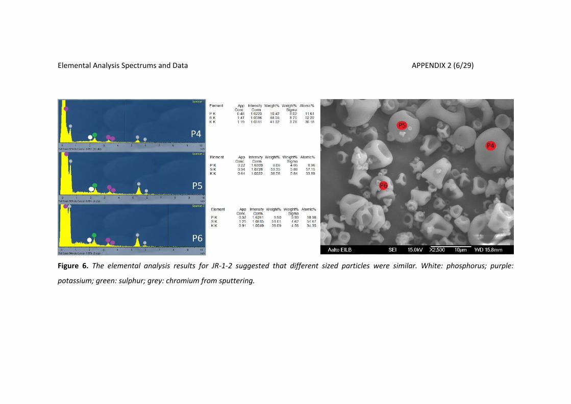
Elemental Analysis Spectrums and Data APPENDIX 2 (6/29)

Figure 6. The elemental analysis results for JR-1-2 suggested that different sized particles were similar. White: phosphorus; purple:

potassium; green: sulphur; grey: chromium from sputtering.

Elemental Analysis Spectrums and Data APPENDIX 2 (7/29)

Figure 7. The elemental analysis results for JR-1-3 suggested that different sized particles were similar .White: phosphorus; purple:

potassium; green: sulphur; grey: chromium from sputtering.

Elemental Analysis Spectrums and Data APPENDIX 2 (8/29)

Figure 8. The elemental analysis for sample JR-1-4 showed that there were differences in sodium and chlorine proportions in different

particles. Smaller particle P12 had Na:Cl ratio closest to 1. Red: chlorine; blue: sodium; white: phosphorus; purple: potassium green: sulphur

grey: chromium from the sputtering.

Elemental Analysis Spectrums and Data APPENDIX 2 (9/29)

Figure 9. The elemental analysis for sample JR-1-4 showed that particles P14 and P15 had similar elemental spectrums. P13 is missing from

the picture Red: chlorine; blue: sodium; white: phosphorus; purple: potassium green: sulphur grey: chromium from the sputtering.

Elemental Analysis Spectrums and Data APPENDIX 2 (10/29)

Figure 10. The elemental analysis results for sample JR-1-5 suggested that larger particles had lower sodium and higher chlorine content.

Red: chlorine; blue: sodium; white: phosphorus; purple: potassium green: sulphur grey: chromium from the sputtering.

Elemental Analysis Spectrums and Data APPENDIX 2 (11/29)

Figure 11. The elemental analysis results from JR-1-6 suggested that smaller particles had higher sodium and lower chlorine content

compared to larger particles. Red: chlorine; blue: sodium; white: phosphorus; purple: potassium green: sulphur grey: chromium from the

sputtering.

Elemental Analysis Spectrums and Data APPENDIX 2 (12/29)

Figure 12. Elemental analysis results did not show significant differences between

particles P1-P3 in sample JR-1-1.

0

20

40

60

P S K

Me

an a

tom

ic p

rop

ort

ion

(%

)

0

20

40

60

80

P1 P2 P3

Ato

mic

pro

po

rtio

n (

%) P

S

K

Elemental Analysis Spectrums and Data APPENDIX 2 (13/29)

Figure 13. Different sized particles seemed to have similar atomic proportions for

sample JR-1-2.

0

20

40

60

80

P S K

Me

an a

tom

ic p

rop

ort

ion

(%

)

0

20

40

60

80

P4 P5 P6

Ato

mic

pro

po

rtio

n (

%) P

S

K

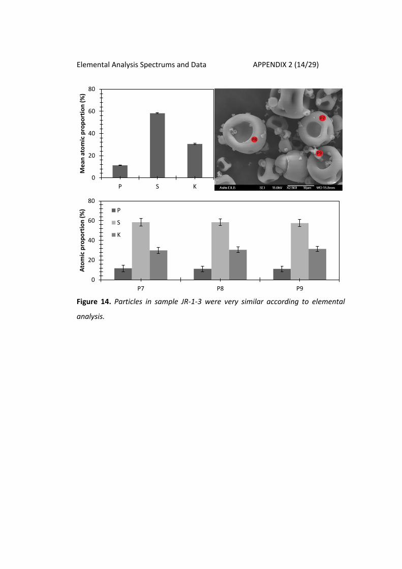
Elemental Analysis Spectrums and Data APPENDIX 2 (14/29)

Figure 14. Particles in sample JR-1-3 were very similar according to elemental

analysis.

0

20

40

60

80

P S K

Me

an a

tom

ic p

rop

ort

ion

(%

)

0

20

40

60

80

P7 P8 P9

Ato

mic

pro

po

rtio

n (

%) P

S

K

Elemental Analysis Spectrums and Data APPENDIX 2 (15/29)

Figure 15. In sample JR-1-4 sodium and chlorine proportions varied significantly

between different particles.

0

20

40

60

80

Na P S Cl K

Me

an a

tom

ic p

rop

ort

ion

(%

)

0

20

40

60

80

P10 P11 P12 P14 P15

Ato

mic

pro

po

rtio

n (

%)

Na

P

S

Cl

K

Elemental Analysis Spectrums and Data APPENDIX 2 (16/29)

Figure 16. The elemental analysis of sample JR-1-5 suggested that different sized

particles had different atomic content. It seemed like the ratio between sodium

and chlorine approached 1:1 when particle size decreased.

0

20

40

60

80

Na P S Cl K

Me

an a

tom

ic p

rop

ort

ion

(%

)

0

20

40

60

80

P19 P20 P21

Ato

mic

pro

po

rtio

n (

%) Na P

S Cl

K

Elemental Analysis Spectrums and Data APPENDIX 2 (17/29)

Figure 17. Sample JR-1-6 showed differences in particle elemental content where

larger particles P22 and P24 showed lower proportion of sodium and lower chlorine

compared to smaller particle P23. Also, particles P22 and P24 had different

morphology but elemental analysis results looked similar.

0

20

40

60

Na P S Cl K

Me

an a

tom

ic p

rop

ort

ion

(%

)

0

20

40

60

P22 P23 P24

Ato

mic

pro

po

rtio

n (

%)

Na P

S Cl

K

Elemental Analysis Spectrums and Data APPENDIX 2 (18/29)

Figure 18. Elemental analysis spectrums and results of sample JR-5-2 (5 % NaCl, pH 5) with 10 000x magnification were taken from several

points to get more reliable results. However, P4 gives differing results. Red: chlorine; blue: sodium; black: aluminum; white: phosphorus;

grey: chromium from the sputtering.

Elemental Analysis Spectrums and Data APPENDIX 2 (19/29)

Figure 19. Clearly differing particle from the sample JR-5-2 (5 % of NaCl, pH 5) was found and analyzed. Red: chlorine; blue: sodium; black:

aluminum; white: phosphorus; purple: potassium; grey: chromium from the sputtering.

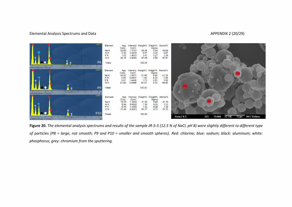
Elemental Analysis Spectrums and Data APPENDIX 2 (20/29)

Figure 20. The elemental analysis spectrums and results of the sample JR-5-5 (12.5 % of NaCl, pH 8) were slightly different to different type

of particles (P8 = large, not smooth; P9 and P10 = smaller and smooth spheres). Red: chlorine; blue: sodium; black: aluminum; white:

phosphorus; grey: chromium from the sputtering.

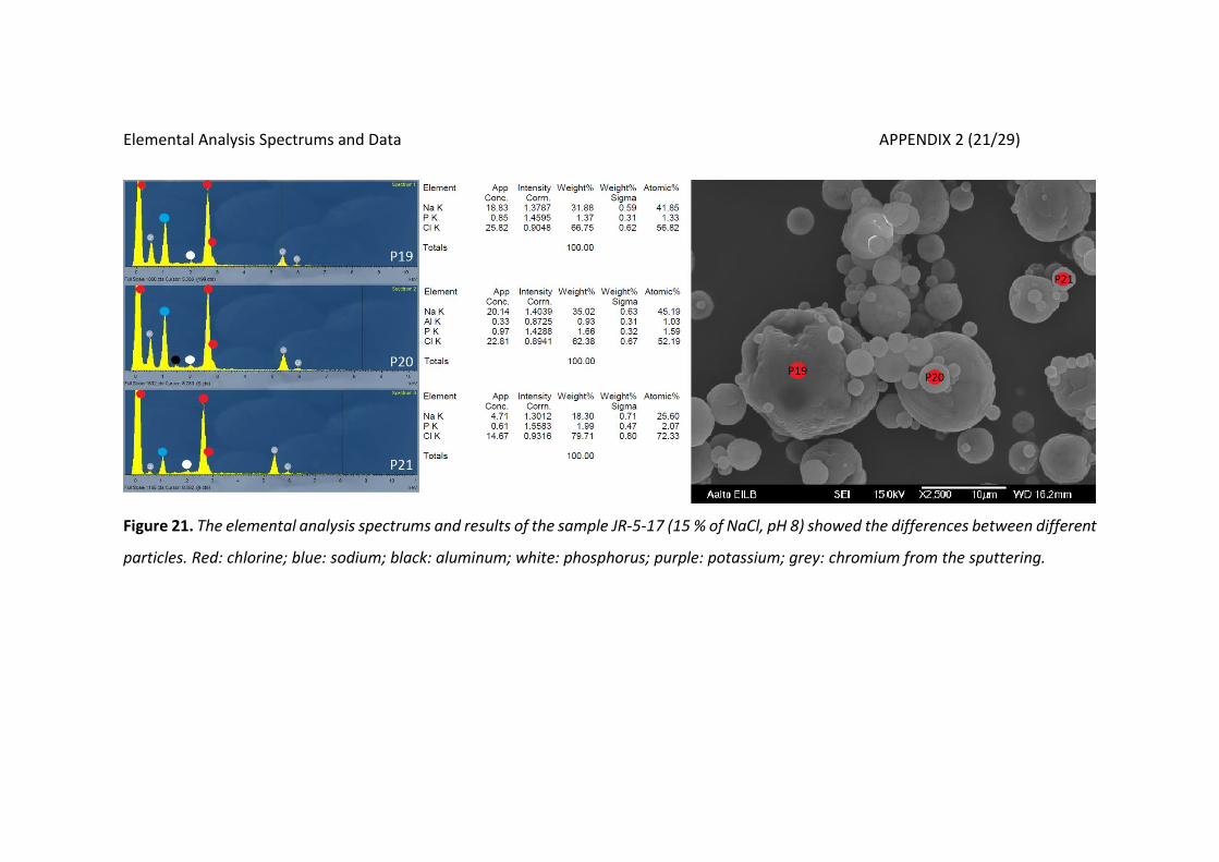
Elemental Analysis Spectrums and Data APPENDIX 2 (21/29)

Figure 21. The elemental analysis spectrums and results of the sample JR-5-17 (15 % of NaCl, pH 8) showed the differences between different

particles. Red: chlorine; blue: sodium; black: aluminum; white: phosphorus; purple: potassium; grey: chromium from the sputtering.

Elemental Analysis Spectrums and Data APPENDIX 2 (22/29)

Figure 22. The elemental analysis spectrums and results of the sample JR-5-9 (12.5 % of NaCl + 2 % Ca-acetate, pH 4.5) suggested that

particles at points P11 and P13, and P12 and P14 were similar. Red: chlorine; blue: sodium; black: aluminum; white: phosphorus; rose:

calcium; grey: chromium from the sputtering.

Elemental Analysis Spectrums and Data APPENDIX 2 (23/29)

Figure 23. The elemental analysis spectrums and results of the sample JR-5-14 (12.5 % of NaCl + 2 % Ca-acetate, pH 8) suggested that

particles at points P15 and P17, and P16 and P18 were similar, but the picture showed different. Red: chlorine; blue: sodium; black:

aluminum; white: phosphorus; rose: calcium; grey: chromium from the sputtering.

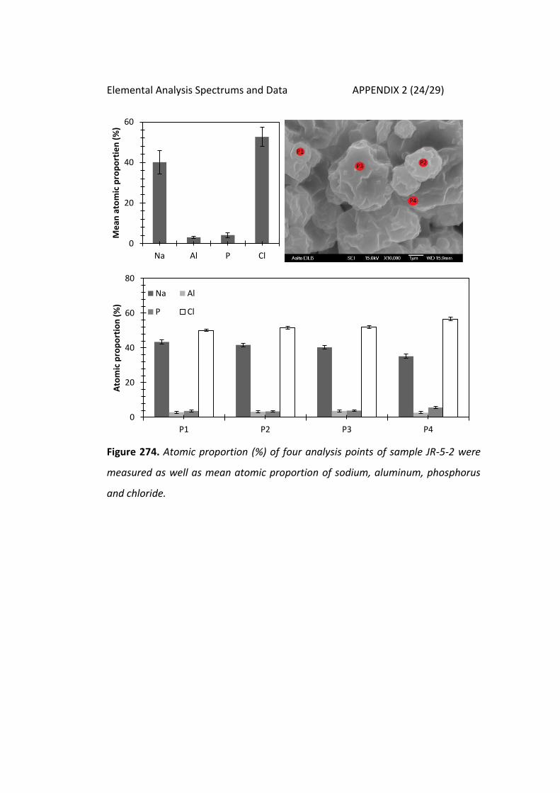
Elemental Analysis Spectrums and Data APPENDIX 2 (24/29)

Figure 274. Atomic proportion (%) of four analysis points of sample JR-5-2 were

measured as well as mean atomic proportion of sodium, aluminum, phosphorus

and chloride.

0

20

40

60

Na Al P Cl

Me

an a

tom

ic p

rop

ort

ien

(%

)

0

20

40

60

80

P1 P2 P3 P4

Ato

mic

pro

po

rtio

n (

%)

Na Al

P Cl

Elemental Analysis Spectrums and Data APPENDIX 2 (25/29)

Figure 285. Atomic proportion (%) of three analysis points of sample JR-5-2 was

measured of differing particle. Also mean atomic proportion of sodium, aluminum,

phosphorus, chloride and potassium was analyzed.

0

20

40

60

80

Na Al P Cl K

Me

an a

tom

ic p

rop

ort

ion

(%

)

0

20

40

60

80

P5 P6 P7

Ato

mic

pro

po

rtio

n (

%)

Na

Al

P

Cl

K

Elemental Analysis Spectrums and Data APPENDIX 2 (26/29)

Figure 26. The results from the elemental analysis of sample JR-5-5 did not show

significant differences between different particles.

0

20

40

60

Na Al P Cl

Me

an a

tom

ic p

rop

ort

ion

(%

)

0

20

40

60

80

P8 P9 P10

Ato

mic

pro

po

rtio

n (

%)

Na Al

P Cl

Elemental Analysis Spectrums and Data APPENDIX 2 (27/29)

Figure 27. Atomic proportion (%) of three analysis points of sample JR-5-17 was

measured. Also mean atomic proportion of sodium, aluminum, phosphorus and

chloride was analyzed.

0

20

40

60

80

Na Al P Cl

Me

an a

tom

ic p

rop

ort

ion

(%

)

0

20

40

60

80

P19 P20 P21

Ato

mic

pro

po

rtio

n (

%)

Na Al

P Cl

Elemental Analysis Spectrums and Data APPENDIX 2 (28/29)

Figure 28. The elemental analysis for the sample JR-5-9 showed aluminum in P12

but the error is relatively large.

0

20

40

60

Na Al P Cl Ca

Me

an A

tom

ic p

rop

ort

ion

(%

)

0

20

40

60

80

P11 P12 P13 P14

Ato

mic

pro

po

rtio

n (

%)

Na Al

P Cl

Ca

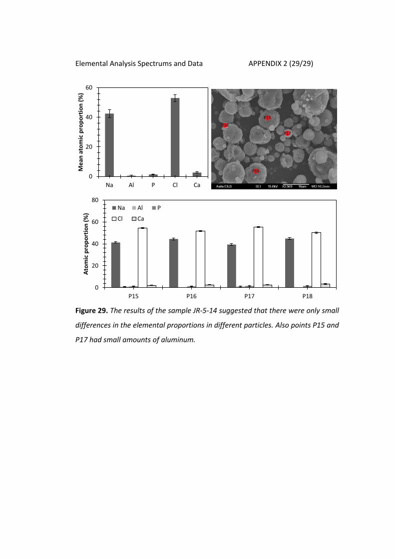
Elemental Analysis Spectrums and Data APPENDIX 2 (29/29)

Figure 29. The results of the sample JR-5-14 suggested that there were only small

differences in the elemental proportions in different particles. Also points P15 and

P17 had small amounts of aluminum.

0

20

40

60

Na Al P Cl Ca

Me

an a

tom

ic p

rop

ort

ion

(%

)

0

20

40

60

80

P15 P16 P17 P18

Ato

mic

pro

po

rtio

n (

%)

Na Al P

Cl Ca

Specific Enzyme Activity Yields APPENDIX 3 (1/1)

Table 17. Results of enzyme 1B activities had problems with the analysis as the

activity yields either are above 100 % or have no consistency. The patterns could

be analyzed for samples with NaCl, and it seemed like the samples with NaCl had

higher activity yields than without NaCl. Methyl cellulose (MC) did not show the

same effect.

NaCl conc. Na2SO4 conc.

Enzyme

solution

conc.

0 % 6.8 % 6.80 % 6.0 % 5 % 4 %

Filtrate

Mix

Concentrate

90.3 %

84.9 %

89.1 %

103.5 %

100.4 %

106.5 %

64.8 %

103.3 %

97.4 %

124.6 %

241.1 %

100.4 %

MC 1,5 % 86.6 %