The Effect of a Low Cost Carrier in the Airline

Industry

By Christine Wang

MMSS Honors Seminar June 6, 2005

*a special thanks to my advisor Ian Savage

2

Table of Contents

Abstract…………………………………………………………....p. 3 I. Introduction………………………………………………...p. 4 II. Deregulation………………………………………………..p. 4-6 III. Effects of Competition on Pricing Behavior…………..…...p. 7-9

A) The Threat of Entry B) Indirect Competition C) Competition of Airports within the same Metropolitan Area

IV. Other Factors Influencing Pricing Behavior……………….p. 10-15 A) Hubs and Market Share B) Price Discrimination

V. The “Southwest Effect”……………………………………p. 15-19 A) Southwest’s Success B) The Definition C) A Study on Southwest

VI. The Analysis…………………………………………...…..p. 19-32 A) The Origins of the Regression B) The Data C) The Estimating Equation D) Descriptive Statistics and Explanation of Coefficients E) Regression without Southwest F) The Magnitude of Southwest’s Effect

VII. The Effect of Southwest Today……………………………p. 32-35 VIII. Conclusion…………………………………………………p. 35 Appendix: Individual Airline Analysis……..………………….…p. 36-38 Works Cited………………………………………………………p. 39

3

Abstract

This paper analyzes the extent of the “Southwest Effect” on the pricing of fares in

the airline industry. First, it discusses the basic principles of pricing under competition,

large market share, and price discrimination. Next, it discusses the role of Southwest in

the airline market. The presence of a low cost carrier, such as Southwest, in a particular

city pair market has long been assumed to lower the fares in that market. This paper

analyzes the extent to which this hypothesis is true. Does the fact that Southwest Airlines

has low fares influence other competitors in that market to lower their fares as well? Or

do the lower fares of Southwest merely lower the average fare in the market? If

Southwest does influence other competitors to lower their fares, does it have more of an

impact on certain airlines? This paper will attempt to answer these questions with

statistical analysis and past literature.

4

I. Introduction

In order to understand the principles of pricing in the airline industry,

knowledge of the industry and its history are essential. There are numerous aspects to

how a plane ticket is priced—how many miles the flight is traveling, when a person buys

his/her ticket, whether the origin and destination airports are hubs, etc. However, one

criteria stands out—the presence of Southwest. With revenues and profits increasing year

to year, Southwest’s success has infiltrated the news and media of the airline industry.

But, what is the cost to its competitors? The following paper will analyze the impact of

Southwest in the airline industry and what this means for the future of all carriers.

II. Deregulation

Since 1938, the U.S. Congress formally regulated air transportation through the

Civil Aeronautics Act. This Act created a board to control the entry and exit of air

carriers, to regulate fares, and to control mergers. However after World War II, an

economic and political consensus1 emerged, claiming that regulation was inefficient and

restricted the growth of the airline industry. These new findings led to the deregulation of

the airline industry in 1978.

The U.S. Domestic Airline Industry was deregulated as part of a reform

movement that has transformed the banking, telecommunications, energy, and

transportation industries in the United States.2 Deregulation was premised on the idea that

an unregulated market would approximate a perfectly competitive industry, one that had

1 Economic studies included Caves 1962, Levine 1965, Jordan 1970, Keeler 1972, and Douglas and Miller 1974. Political support stemmed from Congressional hearings led by Senator Edward Kennedy. 2 Goetz and Sutton; p. 238.

5

numerous carriers, no significant economies of scale, and no significant barriers to entry.

But between 1983 and 1988, the airline industry experienced a massive wave of

bankruptcies, mergers, and acquisitions. Over 200 carriers left the market, leaving nine

airlines (United, American, Continental, TWA, US Air, Pan Am, Delta, Northwest, and

Eastern) to share 92 percent of domestic revenue3. Contrary to initial expectations,

deregulation actually led to a decrease in competition.

Even though deregulation created a more concentrated airline market, it has also

lowered the average airfare and has increased competition on many city-pair routes4.

Moreover, with the allowance of frequent flier plans and discounted fares, U.S. domestic

passenger levels have increased dramatically. From 1978 to 1993, the number of

domestic plane passengers grew from 256 million to 478 million, an 87 percent increase5.

In addition, the frequency in the number of flights has also increased from 5 million flight

departures in 1978 to 7.2 million in 19936. Ordinarily, such growth in demand would

imply positive financial returns; however, the period of deregulation was much less

profitable than in the years prior to deregulation. The situation was so “bleak” that the

Clinton Administration organized the National Commission to Ensure a Strong

Competitive Airline Industry in 1993.

Overall, deregulation of the United States domestic airline industry has had mixed

results. On one hand, people are flying more, average fares are lower, and the number of

flights available has increased. On the other hand, the profits of the industry have greatly

3 Goetz and Sutton; p. 240. 4 U.S. Department of Transportation 1990, U.S. General Accounting Office 1990, National Research Council 1991. 5 U.S. Department of Transportation 1978, 1993. 6 U.S. Federal Aviation Administration 1978, 1993.

6

declined and the industry has become more concentrated. Today, only one or two carriers

dominate specific airports, demonstrating a bias towards the larger airlines. With this

sudden shift in decision-making and control away from government agencies to

individual firms, there is, contrary to the initial expectations of perfect competition, a

possibility of monopolistic behavior. The typical concern with monopolistic behavior is

the fact that it often leads to an increase in price, which then implies a decrease in

consumer surplus and even welfare. However, because the average fare has actually

declined for the industry as a whole, consumer surplus7 has not been adversely affected.

Also, the effect on welfare is ambiguous8. These results can be explained because even

though monopolistic behavior might be expected with the increase in market

concentration, the airline industry is still a competitive industry in the respect that any

airline carrier is allowed to enter the market. Overall, deregulation seems to only benefit

certain groups. It benefits consumers and large airlines, but it also hurts small airlines and

the profitability of the industry as a whole.

7 Consumer surplus is defined as the difference between a consumer’s willingness to pay (height of the demand curve) and what the consumer actually pays. Therefore, if the price of an airline ticket decreases, this increases the difference between the demand curve and the price and consumer surplus increases. 8 Welfare is defined as the sum of consumer surplus and the profit of the industry’s firms. Therefore, even though consumer surplus increases, profit might decrease enough to make welfare decrease. However, if profit does not decrease more than consumer surplus, welfare will increase.

7

III. Effects of Competition on Pricing Behavior

As a result of deregulation, competition in the airline industry is able to act as it

naturally would. In the regular model of perfect competition, the presence of competitors

lowers the price of a particular good for the industry. However, in the case of airline

tickets, the concept of “competition” is unclear since there are a number of different types

of competition. The following is a discussion of these types of competition and whether

each type does indeed lower prices like the model of competition predicts.

A) The Threat of Entry

Since deregulation, a lot has been learned about the “performance characteristics

of airline markets functioning free of government control”9. In a perfectly contestable

market, the threat of entry is said to be sufficient enough to induce competitive pricing.

However, in the studies above, results showed that the airline industry could actually

promote monopolistic behavior. The belief that the airline market conforms to the

contestable markets model has influenced the establishment of a number of policies,

including a number of airline mergers in the 1980’s who expected potential competition

to lower market power in the industry. However, interest in this subject has led to a

number of empirical studies analyzing the extent to which the threat of entry really does

influence market behavior.

One study, performed by Morrison and Winston, found that potential competitors

have a significantly smaller effect on market behavior than actual competitors10. Another

study, performed by Severin Borenstein, found that the effect of potential competitors

9 Peteraf and Reed; p. 193. 10 Morrison and Winston report an insignificant effect of potential carriers until there are at least four potential entrants into the airline industry.

8

may be even less if there are specific carriers who dominate a certain airport11. (A

discussion of Hub Airports will be included later on). Overall, however, the airline

industry does not appear to conform well to the contestable markets model. The threat of

entry is not strong enough to induce either competitive pricing or a less concentrated

market.

B) Indirect Competition

Most of the studies mentioned earlier use a model of large city-pair markets with

multiple competitors. “Considerably less is known about market performance in smaller

markets, especially those in which there is no direct competition”12. However, a few

conclusions have been made about the presence of indirect competition in both large and

small markets.

Indirect competition is defined as the presence of carriers offering service on a

route with at least one stop and a change of planes; whereas direct competition is defined

as the presence of a carrier offering service on a route with no stops or change of planes.

In 1989, Peter Reiss and Pablo Spiller modeled entry into small airline markets with at

most one direct competitor and an unlimited number of indirect competitors13. The results

concluded that indirect competition had a significant effect on market behavior.

However, because indirect service is less desirable than a direct flight, it allows for

product differentiation between carriers and does not influence the market behavior in

exactly the same manner as a perfectly competitive market, with multiple direct

competitors, would. This is due to the fact that airline carriers are able to price

11 Borenstein, The Dominant Firm Advantage. 12 Peteraf and Reed; p. 195. 13 Reiss and Spiller, Competition and Entry in Small Airline Markets.

9

discriminate towards groups that value direct service more highly than indirect service.

Direct service is not the only factor that is affected by price discrimination. Time

valuation (discussed in a later section) is another.

C) Competition of Airports within the same Metropolitan Area

Airports within the same metropolitan area pose the possibility of substitutability

(a passenger might go to another airport if it finds that its carriers offer a lower fare). In

this case, an antitrust analysis was performed which used the cross-elasticity of demand

as the criteria for judging market boundaries14. However, this analysis ignored the

presence of price discrimination and demand segmentation in the airline industry. Since

airlines are allowed to offer restricted discount fares to travelers on the same route at

different times of the day, this enables them to separate out customers by their valuation

of time. Therefore, since business travelers usually book flights that they themselves do

not pay for, we would expect that competing airports would affect the fare of an average

traveler more than that of a business traveler.

Overall, a number of factors influence competition. Some factors even influence

competition on varying levels in different areas of the airline industry. However, the

presence of perfect competition in the deregulated airline market is doubtful. There has

not only been increasing market concentration since deregulation, but also the existence

of monopolistic power in many airports. The next section analyzes other factors that may

influence the pricing behavior of air carriers.

14 Borenstein, Hubs and High Fares: Dominance and Market Power in the U.S. Airline Industry.

10

IV. Other Factors Influencing Pricing Behavior

A) Hubs and Market Share

There are a number of advantages to having airport dominance on a particular

route. The first is that airport dominance enables a carrier to attract more passengers and

raise fares on routes out of that airport because it has a “competitive advantage on routes

that include that airport”15. These competitive advantages arise in two forms. First are

those that occur naturally and second are those that result from programs instituted by

particular airlines. For example, competitive advantage of airport dominance that occurs

naturally is the ability to attract more passengers because it offers the most flights to and

from a city. On the other hand, competitive advantage that occurs through programs

includes frequent-flyer programs and reward systems for travel agents that pay bonuses

when the agent books more flights in favor of one carrier versus another16. In addition, an

airline that dominates a crowded airport may prevent competition by attaining gates and

other physical resources that other airlines need to be competitive. If numerous factors

put a potential entrant at a disadvantage, the carrier may not enter the route market at all

in an effort to avoid difficulties.

Also, using marketing devices that give an advantage to the dominant airline will

increase the number of passengers wanting to fly on that airline. One of the best

marketing devices for this purpose is the use of frequent-flyer programs. “These

programs usually give a gift, usually free travel, to a customer after he or she has

15 Borenstein, Airline Mergers; abstract. 16 Borenstein, Hubs and High Fares: Dominance and Market Power in the U.S. Airline Industry.

11

conducted a certain amount of business with the airline”17. Frequent-flyer programs are

effective in gaining repeat customers because they tend to favor numerous routes from a

customer’s home airport. However, frequent-flyer programs are advantageous only for

large airlines that are able to service a certain number of flights. For smaller airlines, the

number of routes they service is usually not enough to gain repeat customers.

Another advantage is the sunk cost associated with entry. Advertising and the

setup of new airport facilities can be extremely expensive for airlines that are not already

established at a particular airport. Also, when a single airline controls most of the gates at

an airport, it may refuse to sell facilities to entrants or even influence the local

government in deciding whether or not to expand the airport to accommodate new

entrants18. Overall, having airport dominance can lead to an increased market share on

routes that fly into or out of that airport.

Before 1978, the Civil Aeronautics Board attempted to maintain a competitive

balance in the airline industry. However, since then, a proliferation of airport “hubs” has

appeared. A hub is defined as “a control center (airport) that tends to dominate interaction

between direct connections”19. Normally, domestic hubs serve as a major connecting

complex for the airlines. Table 1 shows a list of 22 domestic cities that have been

designated by the carrier as its principal operation center. Between 1978 and 1993, every

domestic hub except for Cleveland experienced an increase in single carrier

concentration20. In 12 of the 22 hubs, one carrier accounted for more than 60 percent of

17 Borenstein, Hubs and High Fares; p. 345. 18 US Department of Transportation, USAir-Piedmont Merger Case. 19 Goetz and Sutton, Deregulation in the Airline Industry; p. 243. 20 Goetz and Sutton, Deregulation in the Airline Industry; p. 244.

12

Table 1: Domestic Hubs of the U.S. Airline Industry21

City/Domestic Hub Major Airlines Atlanta Delta

Baltimore US Air Charlotte US Air Chicago United, American

Cincinnati Delta Cleveland Continental

Dallas-Fort Worth American, Delta, Southwest Denver United Detroit Northwest

Houston Continental, Southwest Las Vegas America West Memphis Northwest

Minneapolis Northwest Nashville American Newark Continental

Philadelphia US Air Phoenix America West Pittsburg US Air

Raleigh-Durham American St. Louis TWA

Salt Lake City Delta Washington United, US Air

the traffic at that airport and in 9 hubs, 70 percent. The development of these hubs

provided a key strategy for major airlines to deter competitive threats from new entrants.

In studies performed by Peteraf, Reiss, and Borenstein, the results showed that

airline share at large airports increases the yields (fare per passenger mile) on routes.

Therefore, there is a direct correlation between airport share and fares. In addition, the

21 Goetz and Sutton, Deregulation in the Airline Industry; p. 243.

13

larger the airline was (i.e. the more market share it possessed), the more likely it is able to

dominate airports and institute programs that reduce competition. If an airline controls a

hub, it often has the pricing power to set higher fares. Another observation is that the

“high markups and fares of the dominant airline do not spill over to smaller airlines

serving the same routes”22. Therefore, only the large firms benefit from hub formation.

Overall, even though hubs create higher fares for consumers who want to fly into

or out of these airports, they also show a more efficient use of aircraft, greater flight

frequency, easier connections, and more nonstop flights associated with these route

systems. There may also be cost savings, which are not fully passed along to consumers,

but still increase total surplus by increasing firms’ profits even though there is a decrease

in consumer surplus23. Therefore, it has been decided by the government that it is overall

unwise to deter such hubs from forming.

B) Price Discrimination

A second factor that influences the pricing behavior of air carriers is price

discrimination. There are two sources of price discrimination in the airline industry. The

first is the different costs associated with serving different passengers. An example of this

is the difference between first class, business, and coach fares. An airline accrues higher

costs in order to provide first class passengers with better food, drinks, service, and

entertainment. Therefore, it will charge a first class passenger a higher fare than a coach

passenger in order to compensate for the higher costs. This type of price discrimination is

22 Borenstein, Hubs and High Fares: Dominance and Market Power in the U.S. Airline Industry; p. 344. 23 As noted above, Total Welfare = Firm Profit + Consumer Surplus. Therefore, an increase in total welfare may still increase as long as either firm profit or consumer surplus increases more than the other declines.

14

associated with a difference in a person’s preference since passengers with higher

incomes are usually willing to pay more for comfort on a flight. The second source of

price discrimination originates from the airline’s effort to predict the demands of different

passengers. This is an example of second degree price discrimination24. In this case,

individual demands are predicted using the time and day of a person’s travel, ticketing

restrictions, or the number of stops on a route. For example, a business traveler25,

characterized as a person who travels during the week departing early in the morning and

arriving back at home in the evening, has a higher willingness to pay because their

companies pay for the flights they are traveling on. On the other hand, a leisure traveler26,

someone who travels during the weekend for pleasure, has a lower willingness to pay.

Therefore, airlines usually will price flights on the same route at different prices

(depending on the day of the week and time) in order to increase profits by extracting

higher prices from people who are willing to pay those prices, while not losing the

business of those who would not pay higher prices.

Though there has been much analysis about the pricing behavior in the airline

industry, one topic is still in need of further analysis. The topic that remains is the impact

of the presence of a low-cost carrier, such as Southwest Airlines, on the pricing behavior

of other airlines. A low cost carrier itself is a specific type of competition in the airline

24 Second degree price discrimination is defined as when the firm sells different units at different prices but it cannot exclude consumers from any offer that it makes. Asher Wolinsky, Economics 350: Monopoly and Competition lecture notes p. 25. 25 A business traveler has a lower demand elasticity and high brand allegiance since even though his/her company pays for the airline ticket, the traveler can accrue advantages such as frequent flier miles in his/her own name. 26 A leisure traveler has a higher demand elasticity and low brand allegiance since these travelers tend to look for the lower fare whether or not that means traveling with the same airline.

15

industry. The rest of the paper analyzes the effect of a low-cost carrier on airline carriers

and the prices they charge.

V. The “Southwest Effect” A) Southwest’s Success27

Southwest Airlines is the fastest growing, most profitable airline in the United

States. In the top 100 domestic markets, which involve over a third of the total number of

domestic travelers, Southwest is the dominant airline, with more passengers than United,

American, and Delta. Southwest’s average market share for its own top 100 markets is 65

percent compared to less than 45 percent for all other airlines. Over the past year,

Southwest has increased its market share in almost all of its top 100 markets and has even

kicked a number of competitors out of those markets. Southwest is known for its high

level of customer service, its reliable on-time arrivals, and most of all, its low fares.

Southwest is categorized into a special niche of airline carriers called LCCs, or low cost

carriers. Other low cost carriers include Jet Blue, Spirit, Air Tran, and WestJet. However,

due to the success and dominance of Southwest Airlines, this paper will focus on

Southwest in particular.

A major difference in the structure of Southwest, in comparison to other major

carriers, is that while other major carriers operate on the hub and spoke system,

Southwest instead operates in “very dense, short haul markets where it can provide

frequent service”28. For example, Southwest dominates the airline market in California,

27 U.S. Department of Transportation, The Airline Deregulation Evolution Continues, The Southwest Effect. 28 U.S. Department of Transportation, The Airline Deregulation Evolution Continues, The Southwest Effect; p. 3.

16

running numerous flights between Northern and Southern California for as low as $29

one way. The typical advantages of an airline hub do not dominate Southwest’s presence

or success in that market. Out of Southwest’s top 100 markets, 82 markets service flights

out of at least 1 hub city and 16 of those markets service flights between 2 hub cities.

Even though those hubs are serviced by other airlines, Southwest has still managed to

increase its market share in those markets. Southwest is also known for its wide

expansion and low operating costs. Compared to other major carriers, Southwest’s

operating costs are about 50 to 70 percent lower. These low costs make it very difficult

for other competitors to remain in the markets served by Southwest.

B) The Definition

The “Southwest Effect”, a term coined by the United States Department of

Transportation in 1993, is based around three principles29. First, the passenger count in a

particular market should increase with Southwest’s presence. The simple logic behind

this being as prices decrease, demand increases and more tickets are being bought for a

particular route. Second, when Southwest enters a market with multiple airports (more

than one airport in a city), the number of passengers that fly into the competing airport

should decrease. For example, since both Midway and O’hare are airports in the city of

Chicago but only Midway is served by Southwest, this should lower the number of

passengers who fly into or out of O’hare. Third, Southwest’s presence in a market should

lower the fares for their competitors in that market in order for their competitors to stay in

competition.

29 Ritter, Southwest Airlines: An In-Depth Review; Chapter 8.

17

C) A Study on the Southwest Effect

A study done at the Embry Riddle Aeronautics University30 focused on the first

and the third principles of the Southwest Effect. It used data from the Origin and

Destination Survey to graph the trends of fare and PDEW (Passengers per Day Each

Way) across time in markets where Southwest had just entered. For example, the

Baltimore-Washington (BWI) to Louisville (SDF) route was added by Southwest in

1994. As Chart 1 indicates, the PDEW averaged 34.2 in 1993 and in 1994, when

Southwest entered, the PDEW jumped to 193.4. Within a year of Southwest’s entry into

the market, the PDEW grew to 322.1. In addition, fares decreased significantly the year

Southwest joined from about $150 to $50. Usually when any carrier adds on a new route,

it offers special fares in order to attract new customers. However, over time, carriers

usually increase their prices to the level of their competitors. An interesting trend to note

about Southwest is that Southwest’s fares begin low but they also stay low. This is the

major difference between Southwest’s pricing behavior compared other competitors’.

Chart 1: Embry Riddle Statistics

30 Ritter, Southwest Airlines: An In-Depth Review; Chapter 8.

18

The conclusions of the study agree with the principles of the Southwest Effect. As

Southwest enters the market, the number of passengers increases and the average fare

decreases. Overall, the study looks at a total of eight different routes where Southwest has

entered the market. Many of the trends resembled those of the BWI to SDF route, though

there were some deviations. The graph for the SEA (Seattle) and SMF (Sacramento)

route show only a slight decline in fares when Southwest entered. Also, the MDW

(Chicago) to HOU (Houston) route showed a decline in prices when Southwest entered,

but then an increase in fares in 1996.

19

Though the prior study does in general agree with the principles of the Southwest

Effect, it yields results for particular routes and does not capture Southwest’s effect on

the airline market as a whole. Also, a graduate student from the Embry-Riddle

Aeronautics University performed the study. The work has not been published and might

not have the academic validity needed to completely support its findings. Most

importantly, this study is flawed in its analysis in the trend of fares. Since Southwest has

lower fares, it is quite obvious that its presence will lower the average fare for the market.

A better question to ask might be: How does Southwest’s presence influence the fares of

its competitors? The rest of the paper focuses on addressing this question with a series of

regressions.

VI. The Analysis

A) The Origins of the Regression

In the basic models of monopoly and competition, price is determined differently

in each case. A monopoly is defined as a sole seller of its product. For each amount of the

product sold, the monopoly can change its price. Therefore, a monopolist is a price setter.

In the case of monopoly, marginal revenue is equal to marginal cost (MR = MC). Price is

determined by the downward sloping demand curve at the quantity where MR = MC.

Chart 2 shows the equilibrium for a monopoly market.

20

Chart 2: Monopoly Equilibrium

For the analysis on Southwest’s effect, the model of competition is of more interest.

The price in perfect competition is determined when P = MC. For the industry as a whole,

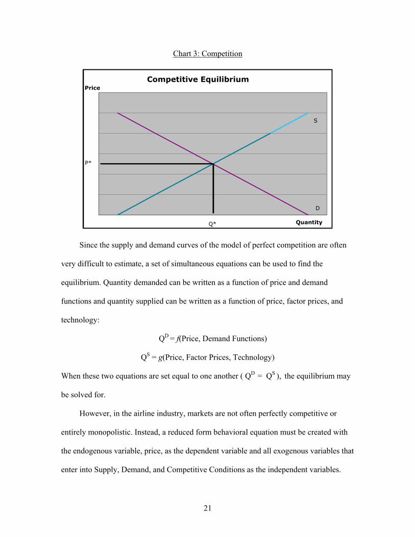
price is determined when demand equals supply (D = S). Chart 3 shows the equilibrium

determined by perfect competition.

When competition occurs, the price of a product is theoretically lower than when

there is a monopoly. The reason being is that when there is a monopoly, firms can charge

up to the highest a consumer is willing to pay, capturing the entire consumer surplus. On

the other hand, in competition, firms are forced to lower their prices in order to gain

customers. Therefore, firms in competition are said to be price takers. In order to capture

the equilibrium from the Supply and Demand curves in the perfect competition model, an

analysis of each curve must be made. However, since the equations of Supply and

Demand are unknown, the best solution is to measure a behavioral reduced form

equation.

Monopoly Equilibrium

MC

DMR

Quantity

Price

P*

Q*

21

Chart 3: Competition

Competitive Equilibrium

Quantity

Price

P*

Q*

D

S

Since the supply and demand curves of the model of perfect competition are often

very difficult to estimate, a set of simultaneous equations can be used to find the

equilibrium. Quantity demanded can be written as a function of price and demand

functions and quantity supplied can be written as a function of price, factor prices, and

technology:

QD = f(Price, Demand Functions)

QS = g(Price, Factor Prices, Technology)

When these two equations are set equal to one another ( QD = QS ), the equilibrium may

be solved for.

However, in the airline industry, markets are not often perfectly competitive or

entirely monopolistic. Instead, a reduced form behavioral equation must be created with

the endogenous variable, price, as the dependent variable and all exogenous variables that

enter into Supply, Demand, and Competitive Conditions as the independent variables.

22

For example, a variable that might enter the demand equation is income. If a

consumer has an increase in income, it is expected that the consumer will buy more

airline tickets, thus increasing demand. For our analysis, the variable INCOMEORIGIN

is included in the regression to account for this trend. On the other hand, a variable that

affects the supply equation might be factor prices such as the price of fuel. When the

price of fuel increases, the supply of flights should decrease. Since it costs more to supply

the good, firms will want to supply less of the good. However, since all air carriers are

affected by the rise in fuel prices, the variable of factor prices is irrelevant for our model.

The literature at the beginning of the paper discusses the different types of

competitive conditions and their effects on price. According to results, the threat of entry

did not prove to have significant effects on the price. Therefore, there is no variable in the

regression used to account for the threat of entry. On the other hand, the other two forms

of competition, indirect competition and multiple airports did show a significant effect on

pricing behavior. Variables were included in the regression to account for these two types

of competition. For indirect competition, the dummy variable NONSTOP was included to

indicate if the ticket was a nonstop itinerary or had one stop or more. For multiple

airports, the variables MULTAIRORIGIN and MULTAIRDEST were included to

account for the presence of multiple airports in either the origin or destination cities.

In addition, the literature discussed two other factors that might influence prices.

The first is the presence of a carrier with large market share. For this factor, the variable

HUB was included in the regression to indicate whether the reporting carrier held a hub

airport for that route. Second, the presence of price discrimination also influenced prices.

For this effect, all travelers of the first type of price discrimination (those who preferred a

23

higher quality of service like those in business and first class) were filtered out. However,

for second degree price discrimination, no data in the data set could be used to account

for whether the traveler was a business traveler or a leisure traveler. Not having this data

available or accounted for in the regression caused there to be ticket-to-ticket price

dispersion found in the analysis and explained why the regression has a low R-squared.

Regardless, the regression did account for a number of other variables involving price

and competition.

The following is an in depth discussion of the data used in the regression and the

estimating equation. It is important to keep in mind that all variables enter the equation as

factors that influence either supply, demand, or competitive conditions. The variable of

interest in this analysis is a fourth type of competition—the effect of a low cost carrier on

pricing behavior. This competition is accounted for with the variable SW and the results

are given in the analysis to follow.

B) The Data

The data used in the analysis comes from the United States Bureau of

Transportation Statistics’ Origin and Destination Survey31. The Origin and Destination

Survey includes a random sample of ten percent of all tickets sold in the United States.

For simplicity, data was filtered out using only the top 50 U.S. domestic markets32 in

Quarter 1 of the year 2004. For cities with multiple airports, all airports for that city were

included as being in the same market. For example, if a top market included a flight

between Chicago and San Jose, flights from both O’hare and Midway to San Jose were

included as being in the same market. In addition, all first-class and business class tickets

31 http://www.bts.gov 32 Transportation Management Consultants: http://www.r2ainc.com/top_us_markets.htm

24

were eliminated from the data in order to prevent an upward bias in fares due to

variations in preferences across consumers. Lastly, all tickets in the database are round

trip tickets33.

C) The Estimating Equation

A log-log cross-sectional regression is used to estimate the various influences of

Southwest’s presence on fares in different markets. The analysis in log-log form was

chosen over both semi log forms because the log-log equation produced a higher R-

squared and more significant t-statistics than the semi log equation. All continuous

independent variables are presented in log form; all dummy variables are not. The final

equation is of the form

ln FAREi = β0 + β1 ln DISTi + β2 ln DISTSQi + β3 NONSTOPi + β4 SWi

+ β5 ln COMPi + β6 MULTAIRORIGINi + β7 MULTAIRDESTi

+ β8 HUBi + β9 ln INCOMEORIGINi + β10 ln COLORIGINi

+ β11 ln POPi + β12 ln WEATHERi + µI

where i is the ith city pair.

The construction of variables is described below.

FARE: The market fare for each non-first-class ticket. These fares are reported from

actual tickets in the O&D Survey.

DIST: The market miles flown on the ticket. For all nonstop service, this was the

mileage between the endpoints of the market. However, for tickets with one stop or more,

33 Tickets that were not round trip tickets were filtered out using the Round Trip Indicator in the database and by merging the Ticket and Market databases in the Origin and Destination Survey.

25

this included the sum of the distance traveled between all airports where the passenger

made a connection.

DISTSQ: The variable DIST to the second power.

NONSTOP: A dummy variable equal to 1 if the ticket is a nonstop flight and 0 if it

is not a nonstop flight.

SW: A dummy variable equal to 1 if Southwest Airlines is present in that particular

market and 0 if it is not present.

COMP: The number of competitors, not including Southwest, in that particular

market. The data for this variable was taken from the Bureau of Transportation Statistics

T-100 Segmented Markets database. Data was sorted by origin and destination and then

the number of reporting carriers was counted to obtain the COMP variable for each

market.

MULTAIRORIGIN: A dummy variable equal to 1 if there is more than one airport

for the origin city and 0 if there is not.

MULTAIRDEST: A dummy variable equal to 1 if there is more than one airport for

the destination city and 0 if there is not.

HUB: A dummy variable equal to 1 if the origin or destination airport was a hub of

the reporting carrier. A list of all the hub airports and their corresponding airline was

found on the Air Traveler’s Handbook 200434.

INCOMEORIGIN: The average income of the origin city.

COLORIGIN: The cost of living index of the origin city.

34 Kantrowitz, The Air Traveler’s Handbook; Part II.

26

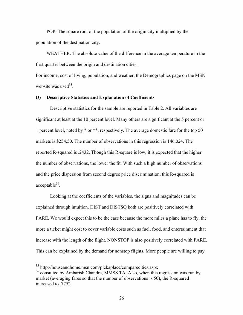
POP: The square root of the population of the origin city multiplied by the

population of the destination city.

WEATHER: The absolute value of the difference in the average temperature in the

first quarter between the origin and destination cities.

For income, cost of living, population, and weather, the Demographics page on the MSN

website was used35.

D) Descriptive Statistics and Explanation of Coefficients

Descriptive statistics for the sample are reported in Table 2. All variables are

significant at least at the 10 percent level. Many others are significant at the 5 percent or

1 percent level, noted by * or **, respectively. The average domestic fare for the top 50

markets is $254.50. The number of observations in this regression is 146,024. The

reported R-squared is .2432. Though this R-square is low, it is expected that the higher

the number of observations, the lower the fit. With such a high number of observations

and the price dispersion from second degree price discrimination, this R-squared is

acceptable36.

Looking at the coefficients of the variables, the signs and magnitudes can be

explained through intuition. DIST and DISTSQ both are positively correlated with

FARE. We would expect this to be the case because the more miles a plane has to fly, the

more a ticket might cost to cover variable costs such as fuel, food, and entertainment that

increase with the length of the flight. NONSTOP is also positively correlated with FARE.

This can be explained by the demand for nonstop flights. More people are willing to pay

35 http://houseandhome.msn.com/pickaplace/comparecities.aspx 36 consulted by Ambarish Chandra, MMSS TA. Also, when this regression was run by market (averaging fares so that the number of observations is 50), the R-squared increased to .7752.

27

a higher price for airline tickets to avoid stops on their routes. HUB is another variable

that is positively correlated to FARE. If the reported carrier has a hub airport in the

market of travel, it can raise prices by the means mentioned in Section IV. Next is

COLORIGIN. The higher the cost of living in a city, the more an airline might be able to

price to that city since the cost to live in that city is already high. Lastly,

INCOMEORIGIN might be positively correlated to FARE because a city with a higher

income can afford to buy more plane tickets (the income effect). If there is a higher

demand for flights, airlines can drive up the price of the tickets they sell.

Aside from all the variables that move together with FARE are the remaining

variables that move negatively with FARE. First, MULTAIRORIGIN and

MULTAIRDEST both move negatively with FARE. This can be explained by the

availability of substitutes. Since a consumer has the option of going to a close airport and

possibly paying a lower fare by doing so, this can cause a downward pressure on the

price of fares offered for the market as a whole. By the same logic, as the number of

competitors increase (COMP), FARE also decreases. This follows from the basic

principles of monopoly and competition37. In addition, as the difference in WEATHER

increases, this might imply that the ticket is bought for leisure travel since business

travelers usually travel to areas with the same temperature. Therefore, as WEATHER

increases, FARE decreases. Next, as POP increases, there is a larger market for airline

travel in that market. A larger market can lead to servicing that market with larger planes.

37 With perfect competition, P=MC whereas with a monopoly, MC=MR. Therefore, monopolists can charge prices as high as the consumer is willing to pay versus when there is perfect competition, firms must charge prices as low as they can without leaving the market.

28

Thus, this might create economies of scale for the airline. With lower variable costs for

the airlines, they may be able to offer passengers lower prices as a result.

Table 2: Statistics

Variable Mean Std. Err. Coef. t-Stat

FARE 254.50 - - -

DIST 1165.07 .004487 .028 6.24**

DISTSQ 1893177.27 .002887 .165 57.17**

NONSTOP .883 .006321 .095 15.04**

SW .41 .0082 -.1825 -22.26**

COMP 3.67 .008918 -.0058 -2.46*

MULTAIRORIGIN .53 .01065 -.0648 -6.09**

MULTAIRDEST .52 .00746 -.0179 -2.40*

HUB 1.13 .00894 .0261 2.41*

INCOMEORIGIN 40,028 .00663 .2169 32.74**

COLORIGIN 130.41 .03548 .0272 7.65**

POP 1889980.32 03667 -.0045 -1.75

WEATHER 17.66 .00376 -.0259 -6.9**

CONSTANT - .27279 .7853 2.88**

* indicates significance at the 5 percent level ** indicates significance at the 1 percent level Out of all the variables, DISTSQ, INCOMEORIGIN, NONSTOP, and SW have

the largest effects on fare. Most importantly, is the large effect of SW on fare. The

presence of SW has an even greater effect than the number of other competitors.

However, the fact that Southwest has a negative effect on fare is obvious. Southwest in

29

itself has very low fares, which would of course lower the average fares in the market

they fly in. In order to see whether Southwest’s presence lowers the fares of other

competitors in the same markets, another regression must be run.

E) Regression without Southwest The exact same regression from part C) was run, however now all the data

involving Southwest as the reporting carrier was taken out of the dataset. Now, the

number of observations is 131,460, the R-squared has increased to .2519, and the average

fare has increased to $276.31. The signs on all the variables remain the same as before,

but there are changes in the magnitudes of the coefficients and in the level of significance

for each variable.

When we look at the statistics for the SW variable, we find that the effect of SW on

FARE is lower than in the previous regression, from a coefficient value of -.1825 to

-.1679. This is expected since the lower fares directly provided by Southwest were

eliminated. However, it is interesting to note that the coefficient is still negative and is

still relatively high compared to the other variables. Even without the Southwest tickets

in the data, SW still has one of the largest effects on FARE. Therefore, it may be

concluded that Southwest’s presence in an airline market does affect the fares of its

competitors. Interestingly enough, SW has an even larger effect than the presence of

other competitors (COMP).

30

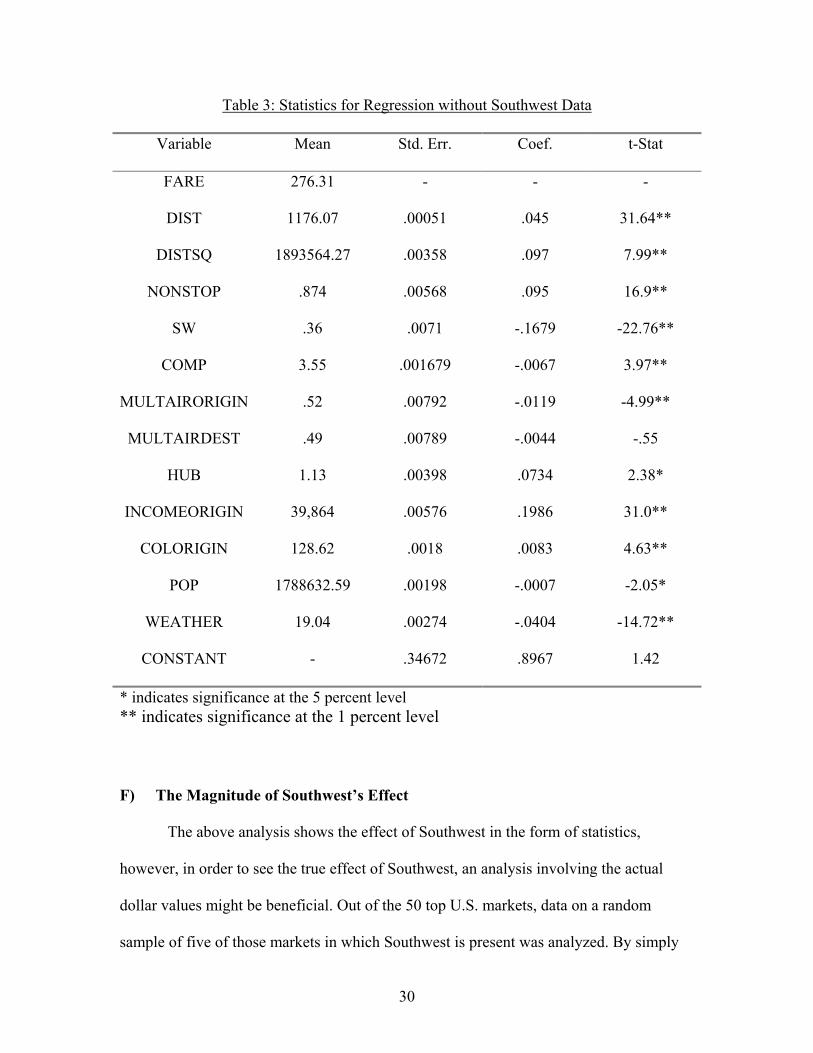
Table 3: Statistics for Regression without Southwest Data

Variable Mean Std. Err. Coef. t-Stat

FARE 276.31 - - -

DIST 1176.07 .00051 .045 31.64**

DISTSQ 1893564.27 .00358 .097 7.99**

NONSTOP .874 .00568 .095 16.9**

SW .36 .0071 -.1679 -22.76**

COMP 3.55 .001679 -.0067 3.97**

MULTAIRORIGIN .52 .00792 -.0119 -4.99**

MULTAIRDEST .49 .00789 -.0044 -.55

HUB 1.13 .00398 .0734 2.38*

INCOMEORIGIN 39,864 .00576 .1986 31.0**

COLORIGIN 128.62 .0018 .0083 4.63**

POP 1788632.59 .00198 -.0007 -2.05*

WEATHER 19.04 .00274 -.0404 -14.72**

CONSTANT - .34672 .8967 1.42

* indicates significance at the 5 percent level ** indicates significance at the 1 percent level

F) The Magnitude of Southwest’s Effect

The above analysis shows the effect of Southwest in the form of statistics,

however, in order to see the true effect of Southwest, an analysis involving the actual

dollar values might be beneficial. Out of the 50 top U.S. markets, data on a random

sample of five of those markets in which Southwest is present was analyzed. By simply

31

using the above regression, with the coefficients substituted in, the fare with Southwest

(SW = 1) and without Southwest (SW = 0) was found for each market. The results are

shown in Table 4 and Chart 4.

Table 4: Dollar Magnitudes of the Southwest Effect

Route Fare with Southwest (SW = 1)

Fare without Southwest (SW = 0)

Dollar Increase Percent Change

MDW:DFW $202.62 $242.64 $40.02 +19.75%

LAX:JFK $317.72 $380.89 $63.17 +19.88%

FLL:LGA $236.54 $283.89 $47.35 +20.02%

LAS:LGA $328.19 $393.90 $65.71 +20.02%

DTW:MCO $217.52 $261.07 $43.55 +20.02%

Chart 4: Dollar Differences of the Southwest Effect

0

50

100

150

200

250

300

350

400

Pri

ce i

n d

oll

ars

MDW:DFW LAX:JFK FLL:LGA LAS:LGA DTW:MCO

Route

w/ Southwest

w/o Southwest

32

As results indicate, the absence of Southwest in each market increases fares by

about 20%. Not only is the coefficient on the Southwest variable significant, but its effect

on the dollar magnitude is also quite large.

VII. The Effect of Southwest Today

During the first week of January 2005, the effects of Southwest were directly

seen when Delta Airlines announced its “SimpliFares” plan. With a new pricing scheme

that is supposed to mimic those of low-cost carriers, Delta streamlined and cut domestic

fares practically overnight. The new pricing policy included capping unrestricted one-

way fares at $499 for economy travelers and at $599 for business travelers. It lowered the

ticket change fee from $100 to $50. And finally, it eliminated the Saturday stay-over

requirements. In response to Delta’s new pricing structure, nearly all major airlines

followed in the same pattern, though some were more drastic than others. The following

is the chain reaction that resulted in Delta’s new pricing behavior38:

AirTran- Said its fares are already lower than Delta's.

Northwest- Made limited adjustments in select markets shared with Delta.

Southwest- Said its fares are already lower than Delta's.

American- Matched or exceeded Delta's changes in selected markets.

Continental- Made limited adjustments in select markets shared with Delta.

United- Made limited adjustments in select markets shared with Delta.

US Airways- Made limited adjustments in select markets shared with Delta.

Even though a number of the major airlines are making progress in their pricing

behavior, many people remain skeptic to the change. First, the fare cuts position the

38 Armstrong, The San Francisco Chronicle.

33

major airlines closer to the low cost airlines in the prices they charge; however, the

operating costs of the major airlines still remain much higher than those of Southwest and

Jet Blue. Some analysts think that the new pricing structure could cost airlines between

$2-$3 billion in short term revenue loss39. Second, though the lower prices do help a

number of people get a better deal on their airline tickets, “the deep price cuts highlighted

by Delta and American benefit a relatively small percentage of travelers”40. Prices on

routes dominated by one carrier still remain high and tickets with the greatest discounts

usually are scheduled for Tuesdays and Wednesdays, the two least popular days of the

week to travel. Moreover, the new plan also benefits those travelers who book flights at

the last minute (business travelers) more than those who book ahead (leisure travelers).

Chart 5 shows the average percentage drops in fares for both leisure and business

Chart 5:Fare Changes for Business and Leisure Travelers41

The Percent Change in Fares by Airline

-45%

-40%

-35%

-30%

-25%

-20%

-15%

-10%

-5%

0%

5%American Continental Delta Northwest United US Airways

AmericaWest

LeisureBusiness

39 Armstrong, The San Francisco Chronicle. 40 Adams, USA Today. 41 Adams, USA Today.

34

travelers. As the chart indicates, the drop in business fares is much higher than the drop in

leisure fares for five out of the seven airlines represented below. With all of the reasons

discussed above, many people argue that discounters such as Southwest are still the best

in providing the lowest fares for the largest percentage of the flights they serve.

It is quite obvious that Southwest has had an enormous effect on the airline

industry. Last year, Delta Airlines posted a record $5.2 billion loss for the year 2004.

Delta CEO Jerry Grinstein says “a traditional carrier like his has no choice but to

embrace elements of the simple, low-fare airline business model that has brought success

to discounters like Southwest and Jet Blue”42. Under the pressures of rising fuel prices

and the entrance of low cost carriers, many carriers have been forced to file for

bankruptcy. However, even though major carriers are now trying to compete with lower

fares, the cost structure of the major airlines might not be able to handle the cut in

revenue. For the first quarter of 2005, Delta still reported major losses of $1.1 billion.

Though more people are flying on Delta, the increase in the number of tickets does not

make up for the high costs associated with the flights.

As for Southwest, quite the opposite has occurred. In the year 2003, Southwest

earned over $442 million in revenue, more than all other U.S. competitors combined. It

boarded the most domestic travelers of any other airline and landed in the top ten of

FORTUNE magazine’s Most Admired Companies. It is not a surprise that the analysis of

this paper concludes that Southwest has a profound impact on the lower prices of the

markets it flies in. However, it is important to note that there are limitations in how low

the prices can go. With the high cost structures of Delta, American, United, and all other

42 Adams, USA Today.

35

major carriers, lowering their fares might entail losses in revenue that the airlines cannot

endure. Instead, airlines like US Airways have either lowered or completely eliminated

the number of flights they serve in markets with Southwest. Over time, the “Southwest

Effect” has become more and more dominant and its stronghold on the airline industry

will continue to influence airline prices, markets, and competitors.

VIII. Conclusion

Overall, the “Southwest Effect” has proved to be very dominant in the airline

industry. It has not only lowered the average fare in the markets it serves, but it also has

induced other carriers to lower their fares in those markets. Year after year, Southwest

increases its market share and expands the number of routes that it services. With United

filing for bankruptcy a couple years ago and Delta close on its way, analysts have begun

to wonder if Southwest will become the new Microsoft. Will Southwest’s fares become

so low that it will virtually make competition in the airline industry impossible? As

Southwest moves to monopolize more and more routes, will its competitors be forced to

change its cost structure? The answers to these questions remain in the future of the

airline industry and in the future of low cost carriers.

36

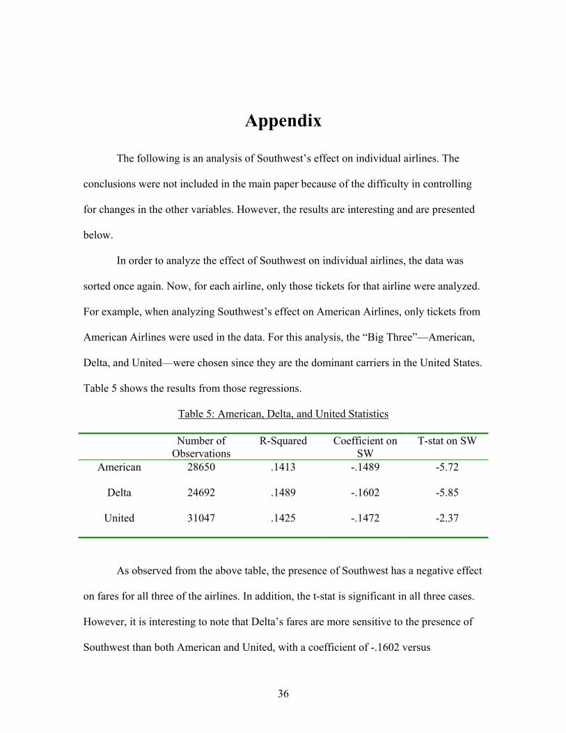
Appendix

The following is an analysis of Southwest’s effect on individual airlines. The

conclusions were not included in the main paper because of the difficulty in controlling

for changes in the other variables. However, the results are interesting and are presented

below.

In order to analyze the effect of Southwest on individual airlines, the data was

sorted once again. Now, for each airline, only those tickets for that airline were analyzed.

For example, when analyzing Southwest’s effect on American Airlines, only tickets from

American Airlines were used in the data. For this analysis, the “Big Three”—American,

Delta, and United—were chosen since they are the dominant carriers in the United States.

Table 5 shows the results from those regressions.

Table 5: American, Delta, and United Statistics

Number of Observations

R-Squared Coefficient on SW

T-stat on SW

American 28650 .1413 -.1489 -5.72

Delta 24692 .1489 -.1602 -5.85

United 31047 .1425 -.1472 -2.37

As observed from the above table, the presence of Southwest has a negative effect

on fares for all three of the airlines. In addition, the t-stat is significant in all three cases.

However, it is interesting to note that Delta’s fares are more sensitive to the presence of

Southwest than both American and United, with a coefficient of -.1602 versus

37

American’s coefficient of -.1489 and United’s coefficient of -.1472. Though the

coefficients for each airline are still large, it may be asked why Delta’s fares are more

sensitive than both American’s and United’s.

One reason Delta’s fares may be more sensitive than both American and United is

that American and United are already sensitive to competition with other airlines. Table 6

shows the number of routes served by the four airlines—American, Delta, United, and

Southwest. For example, 79 indicates the number of routes serviced by both Delta and

American. From the chart, American and United compete with one another the most out

of all four airlines. For American, 135/648, or about 20.83%, of its routes are in

competition with United. For United, an even larger percentage of about 30.33% of its

routes are shared with American. As for Delta, only 17.55% of its routes are in

competition with American and an even lower 5.55% of its routes are in competition with

Table 6: Number of Routes by Carriers43

American Delta United Southwest

American 382 79 135 52

Delta 79 450 25 58

United 135 25 262 23

Southwest 52 58 23 734

Total 648 612 445 867

43 The number of routes was calculated using the t-100 database from the Bureau of Transportation Statistics. The t-100 encompasses all routes inside the United States. Note that by “route”, a specific origin and destination are implied. For example, a route may be all flights from LAX to JFK, but all flights from JFK to LAX are not included as being in the same route. For all flights between LAX and JFK, no matter what the origin and destination may be, the term “market” is used for this paper.

38

United. Part of this may be due to the fact that American and United share one of the

largest hub airports with one another—O’hare International Airport. In addition, since so

few of Delta’s routes are shared with the top competitors, Delta might have a majority of

monopolistic routes from a number of its own hub airports such as Cincinnati (CVG) or

Atlanta (ATL). Since American and United already are in great competition with one

another, their fares may already be lower. Therefore, when the presence of Southwest is

taken into account, Delta’s fares could be more sensitive to SW and less sensitive to other

competitors. This reasoning does hold ground because in the regression statistics, both

American and United had more sensitive coefficients to competition than Delta.

Though the presence of more competitors may be one reason why Delta is more

sensitive to Southwest, another reason might be Delta’s quicker response to pricing

policies. Recently, Delta has instituted new fare cuts in order to position itself closer to

the fares of low-cost carriers such as Southwest and Jet Blue Airlines. Since Delta’s

announcement to cut fares, there has been a “chain of responses by some of its

competitors”44. Though its price cuts were created in the beginning of 2005 and the data

used in this analysis originates from the first quarter of 2004, Delta’s willingness to cut

prices and aggressive pricing policies may have rivaled those of American and United

over a year ago. Overall, there are a number of factors that could influence Delta being

more sensitive to Southwest’s presence than American and United. Unfortunately, not

enough information is known about Delta’s pricing strategies to reach a clear conclusion

about why that might be.

44 Armstrong, The San Francisco Chronicle.

39

Works Cited

Adams, Marilyn. “Simplified ticketing is not so simple for all travelers.” USA Today. February 2005. <http://www.usatoday/money/biztravel.com>.

Armstrong, David. “Straightforward fares: Delta sparks overhaul of airline pricing

policies.” The San Francisco Chronicle. January 2005. <http://sfgate.com>. Borenstein, Severin. “Hubs and High Fares: Dominance and Market Power in the U.S.

Airline Industry.” The RAND Journal of Economics. Autumn 1989. Borenstein, Severin and Rose, Nancy. “Competition and Price Dispersion in the U.S.

Airline Industry.” The Journal of Political Economy. August 1994. The Bureau of Transportation Statistics. The Origin and Destination Database and The t-

100 Segmented Markets Database. Quarter 1, 2004. <www.bts.gov>. Goetz, Andrew and Sutton, Christopher. “The Geography of Deregulation in the U.S.

Airline Industry.” Association of the American Geographers. June 1997. Kantrowitz, Mark. “Air Traveler’s Handbook.” Carnegie Mellon University. June 2004.

<http://www.faqs.org/faqs/travel/air/handbook/part2/section-13.html>. Morrison, S. and Winston, C. “Empirical Implications and Tests of the Contestability

Hypothesis.” Journal of Law and Economics. April 1987. MSN.COM. <http://houseandhome.msn.com/pickaplace/comparecities.aspx>. Peteraf, Margaret and Reed, Randal. “Pricing and Performance in Monopoly Airline

Markets.” Journal of Law and Economics. April 1994. Reiss, P. and Spiller Pablo. “Competition and Entry in Small Airline Markets.” Journal

of Law and Economics. October 1989. Ritter, Justin. “Southwest Airlines: An In-Depth Review.” Embry-Riddle Aeronautics

University Chapter 8. Transportation Management Consultants. “Top 50 U.S. Domestic Markets.” U.S

Department of Transportation Data Base Products, Inc. <http://www.r2ainc.com/ top _us_markets.htm>.

U.S. Department of Transportation. “The Airline Deregulation Evolution Continues: The Southwest Effect.” Office of Aviation Analysis, Washington D.C.

Wolinsky, Asher. “Monopoly and Competition.” Northwestern University. Evanston, IL.

Winter 2005.