The Economics of Climate Change Legislation in North Carolina€¦ · The Economics of Climate...
73
The Economics of Climate Change Legislation in North Carolina David G. Tuerck, PhD Paul Bachman, MSIE Alfonso Sanchez-Penalver, MSF Michael Head, MSEP THE BEACON HILL INSTITUTE AT SUFFOLK UNIVERSITY 8 Ashburton Place Boston, MA 02108 Tel 617-573-8750, Fax 617-994-4279 Email [email protected] , Web; www.beaconhill.org April 2008
Transcript of The Economics of Climate Change Legislation in North Carolina€¦ · The Economics of Climate...

The Economics of Climate Change Legislation in North Carolina
David G. Tuerck, PhD Paul Bachman, MSIE Alfonso Sanchez-Penalver, MSF Michael Head, MSEP
THE BEACON HILL INSTITUTE AT SUFFOLK UNIVERSITY 8 Ashburton Place Boston, MA 02108 Tel 617-573-8750, Fax 617-994-4279 Email [email protected], Web; www.beaconhill.org April 2008
Table of Contents
Executive Summary ......................................................................................................2 Introduction...................................................................................................................6
The CAPAG Report.................................................................................................8 The ASU Report......................................................................................................9 North Carolina-STAMP.........................................................................................11
Eight CAPAG Recommendations...............................................................................12 Energy Demand and Supply...................................................................................12 Energy Demand .....................................................................................................13 RCI-1: Demand Side Management Programs ........................................................13 RCI-2: Expand Energy Efficiency Funds................................................................13 ES-7: Public Benefits Charge ................................................................................14 Energy Supply .......................................................................................................14 Transportation .......................................................................................................15 TLU-5: Tailpipe GHG standards ...........................................................................15 TLU-3a: Surcharges to Raise Revenue...................................................................15 TLU-6: Biofuels Bundle .........................................................................................16 ES-4: Cap and Trade..............................................................................................16
BHI Estimates and Results .........................................................................................18 Energy Demand and Supply...................................................................................18 Transportation .......................................................................................................20 Cap and Trade .......................................................................................................22
Conclusion ...................................................................................................................25 Appendix A: Simulation Methodology ......................................................................26 Appendix B: NC-STAMP...........................................................................................33 Bibliography ................................................................................................................68
Table of Tables
Table 1: CAPAG Estimates 2007-2020 ...........................................................................3 Table 2: ASU Cumulative Estimates to 2020...................................................................4 Table 3: Summary of BHI Estimates for 2011 .................................................................5 Table 4: CAPAG Policy Recommendations for BHI Simulations ..................................12 Table 5: Economic and Fiscal Impact of Energy Sector Recommendations....................19 Table 6: Economic and Fiscal Impact of CAPAG Transportation Sector Proposals........21 Table 7: Economic and Fiscal Impact of Cap and Trade ................................................23 Table 8: Government Sectors.........................................................................................39 Table 9: Industry Elasticities .........................................................................................63 Table 10: Household Related Elasticities.......................................................................64 Table 11: Summary of Set Names .................................................................................65 Table 12: Summary of Parameter Names.......................................................................66
Executive Summary In 2005, the North Carolina Legislature approved Session Law 2005-442, which established the
Legislative Commission on Global Climate Change (LCGCC). The Commission’s mandate was
to “study issues related to global warming, the emerging carbon economy, and whether it is
appropriate and desirable for the state to establish a global warming pollutant reduction goal.”1
A separate but overlapping organization is the North Carolina Climate Action Plan Advisory
Group (CAPAG), which describes itself as “a voluntary advisory group to the NC Department of
Environment and Natural Resources (DENR) … administered by its Division of Air Quality
(DAQ) with assistance and facilitation from the Center for Climate Strategies (CCS).”2 CAPAG
charged itself with developing an action plan with recommendations to reduce the state’s
greenhouse gas emissions, coordinating with the LCGCC in the process.
In October 2007, CAPAG released a draft final report that offers 56 recommendations for
reducing GHG emissions covering four sectors of the state economy. The report provides
estimates of the amount of the GHG reduction and estimates of the net present value (NPV) of the
costs, or cost savings, of implementation. According to the report, the implementation of all 56
proposals would reduce GHG emissions in North Carolina by 827.7 million metric tons of carbon
dioxide equivalent (MMtCO2e) between 2007 and 2020.3
Table 1 summarizes the estimated reduction in total emissions and the professed cost savings for
eight of CAPAG’s 56 recommendations. The recommendations fall into three categories –
Energy Demand and Supply, Transportation and Cap and Trade. We choose the
recommendations falling into these categories because they are responsible for more than half the
promised GHG emission reductions and most of the cost savings claimed by CAPAG. According
1 General Assembly of North Carolina, An Act to Establish the Legislative Commission on Global Warming, S 1134, Session Law 2005-442 (September 27, 2005). http://www.ncleg.net/gascripts/DocumentSites/browseDocSite.asp?nID=14&sFolderName=\Authorizing%20Legislation. See also An Act to Extend the Legislative Commission on Global Warming, S 1591 S.L. 2006-73 (July 10, 2006), http://www.ncleg.net/documentsites/committees/LCGCC/Authorizing%20Legislation/SL%202006-73%20LCGCC%20ext%20auth.pdf. 2 Memo from The Center for Climate Strategies to North Carolina Climate Action Plan Advisory Group, February 16, 2006, http://www.ncclimatechange.us/capag.cfm. 3 North Carolina Climate Action Plan Advisory Group, “Recommended Mitigation Options for Controlling Greenhouse Gas Emissions: Draft Final Report” (October 2007), http://www.ncclimatechange.us/capag.cfm; 1-11.

The Economics of Climate Change Legislation in North Carolina/ April 2008 3
to CAPAG, all eight recommendations would reduce GHG emissions by 465.5 MMtCO2e
between 2007 and 2020. Moreover, the reduction in GHG would be accompanied by net savings
of $5,708.2 million, in present value terms, to North Carolina citizens.
The energy demand and supply proposals include an “Environmental Portfolio Standard” that
would mandate a specified percentage of renewable energy production in the electricity sector;
create new Public Benefit Charges on electricity use; and dedicate a portion of private utility
revenues to energy efficiency programs to reduce demand. CAPAG estimates that these
proposals would reduce GHG emissions by 322.5 MMtCO2e and confer net cost savings of about
$2.5 billion between 2007 and 2020.
Table 1: CAPAG Estimates 2007-2020
Recommendation Reduction
(MMtCO2e) NPV of Cost Change
($, million) Energy Demand and Supply 322.5 - 2,502.2 Transportation 95.6 - 3,490.0 Cap and Trade 47.4 284.0 Total 465.5 - 5,708.2
The CAPAG recommendations for the transportation sector include a “Biofuels Bundle” that
would mandate targets to increase ethanol use in gasoline and diesel fuel, implement a proposal to
adopt California Emission Standards on light duty vehicles and set new registration fees for
vehicles based on emissions output. These proposals would reduce emissions by 95.6 MMtCO2e
and save North Carolinians $3.5 billion.
CAPAG also proposes to include North Carolina in a regional or national system to cap GHG
emissions and issue tradable permits that allow businesses in specified industries to emit
greenhouse gases. According to CAPAG, the system would reduce emissions by 47.4 MMtCO2e
and cost $284 million.
While CAPAG was doing its work, researches at Appalachian State University Energy Center
(ASU) produced their own estimates of the economic effects of 31 CAPAG recommendations.
The ASU researchers utilized the North Carolina Energy Scenario Economic Impact Model (NC-
ESEIM), which was developed to quantify the potential impacts on the state economy of major
energy policy initiatives designed to reduce greenhouse gas emissions. They reported that, over

The Economics of Climate Change Legislation in North Carolina/ April 2008 4
the period 2007 to 2020, the CAPAG policy measures would increase employment in the state by
328,738 jobs, boost income by just over $14.2 billion, and raise value added by over $20.5
billion.4
Table 2 provides details of the ASU results broken out by category. Seven proposals that target
energy supply would, according to ASU, create 46,000 jobs and increase incomes in North
Carolina by over $3.1 billion. Fourteen proposals attempt to reduce emissions by reducing
energy demand and would add 133,000 jobs and boost incomes by $4.6 billion. Ten proposals
would reduce GHG emissions by altering the state’s agriculture, forestry policies and waste
disposal policies, which are expected to create almost 150,000 jobs and add $6.5 billion to
income.
Table 2: ASU Cumulative Estimates to 2020
Recommendation Employment
(Jobs) Income
($ millions) Value Added ($ millions)
Energy Demand Proposals 132,985 4,632 4,449 Energy Supply Proposals 45,996 3,122 5,887 Agriculture &Forestry and Waste Proposals 149,757 6,455 10,225 Total 328,738 14,209 20,561
The CAPAG and ASU scenarios do not stand up to scrutiny. The cost-benefit methodology
employed by CAPAG suffers from three serious problems: CAPAG (1) failed to quantify benefits
in a way (dollar terms) that can be meaningfully compared to costs, (2) misinterpreted costs to be
benefits and (3) understated the true costs of its recommendations.
The ASU report also contains serious methodological flaws. The use of a multiplier analysis is
not appropriate. The model does not allow the changing price of electricity to affect production
or determine the price deflator (inflation) component of state Gross Domestic Product (GDP),
with the result that GDP is projected to vary directly with electricity costs. The assumptions
about what determines investment – the key driver of this input-output model – are too optimistic.
Finally, the assumptions about the evolution of energy costs (particularly the sharp drop in the
cost of renewable energy) over time are implausible.
4David Ponder and Jeffry Tiller, “Preliminary Draft Results, Economic Impact Analysis of Bundled Climate Mitigation Options: Prepared for the North Carolina Climate Action Advisory Group,” October 27, 2007, PowerPoint Presentation.

The Economics of Climate Change Legislation in North Carolina/ April 2008 5
The John Locke Foundation contracted with the Beacon Hill Institute (BHI) to provide
independent estimates of the economic and fiscal impact of selected CAPAG proposals. To that
end, BHI constructed a STAMP® (State Tax Analysis Modeling Program) for North Carolina
(NC-STAMP), with which we estimated the economic effects of the eight CAPAG
recommendations.5 We assume that the proposals become effective in 2008, and we report
results through 2011. Table 3 summarizes the results for 2011, again with the eight
recommendations combined into three categories.
Table 3: Summary of BHI Estimates for 2011
Recommendation
Net Employment
(Jobs) Investment ($millions)
Real Disposable Income
($ millions)
Real State GDP
($ millions)
State and Local Revenue
($ millions) Energy Demand & Supply (2,473) (76.7) (242.5) (360.3) 170.3 Transportation (1,202) (27.7) (46.5) (168.0) (17.5) Cap and Trade (29,808) (397.9) (1,976.5) (4,002.6) (337.3) Total* (33,483) (502.4) (2,265.5) (4,530.9) (184.6) *Minor differences are due to rounding.
We find that the proposals would exert significant negative effects on the state economy. By
2011, the state would shed more than 33,000 jobs. Annual investment would drop by about
$502.4 million, real disposable income by more than $2.2 billion and real state Gross Domestic
Product (GDP) by about $4.5 billion. The energy Cap and Trade system causes most of the harm.
The negative economic effects would spill over into state and local tax collections. We estimate a
loss of $184.6 million in revenues in 2011.
The proposals’ negative economic and fiscal effects stem from the price and tax increases they
would impose on the energy and transportation sectors. Our results contrast with the positive
results produced by CAPAG and ASU, which suffer from the previously-described deficiencies.
5 Detailed information about the North Carolina -STAMP® model can be found in Appendix B

The Economics of Climate Change Legislation in North Carolina/ April 2008 6
Introduction The debate concerning the environmental and economic impacts of global climate change has
intensified in recent years. This development has encouraged many state governments to
consider public policy initiatives designed to address climate-related issues. The initiatives focus
particularly on the mitigation and reduction of Greenhouse Gasses (GHG) through the
development and implementation of state-level climate action plans.
Prior to the authorization and establishment of climate action plans, state legislatures usually
establish preliminary fact-finding commissions to determine the most beneficial strategies for
mitigating GHG emissions. In North Carolina, the Clean Smokestacks Act of 2002 (CSA)
required the Department of Environment and Natural Resources and the Division of Air Quality
(DAQ) to submit a report to the Environmental Management Commission (EMC) and the
Environmental Review Committee (ERC) of the General Assembly.
In 2005, the Department of Environment and Natural Resources and the Division of Air Quality
submitted a report to the General Assembly in which they attempted to identify and evaluate
strategies for the reduction of GHG emissions. In addition to the recommendations for potential
state actions, the Division of Air Quality provided an inventory and forecast of GHG emissions
from 1990-2020 for the state of North Carolina.
More importantly, the report advocated the formation of a DAQ stakeholder process that would
work further to develop specific policy actions for the reduction of GHG emissions. Furthermore,
the report recommended that the stakeholders compile the findings of this process in a climate
action plan that would guide the GHG mitigation planning of North Carolina policymakers.
Subsequent to the 2005 release of the DAQ report, the General Assembly created the North
Carolina Legislative Commission on Global Climate Change (LCGCC). The questions of
whether a reduction in GHG emissions constitutes a sensible policy goal and, if so, what
comprises the optimal level of GHG reductions were among the fact-finding mandates imposed
by the General Assembly on the LCGCC.

The Economics of Climate Change Legislation in North Carolina/ April 2008 7
The proceedings of the LCGCC have transpired concurrently and often in cooperation with other
facets of the GHG planning process, including other state agencies such as the DENR and DAQ.
A voluntarily formed stakeholder group known as the North Carolina Climate Action Plan
Advisory Group (CAPAG) has been particularly influential in the process; it shares participants
with the LCGCC and submits its findings for consideration to the Commission. CAPAG
describes itself as “a voluntary advisory group to the NC Department of Environment and Natural
Resources (DENR) … administered by its Division of Air Quality (DAQ) with assistance and
facilitation from the Center for Climate Strategies (CCS).”6 While the LCGCC and CAPAG
comprise formally independent and separate entities, both groups have exhibited a substantial
willingness to cooperate in the GHG planning process.
In October 2007, CAPAG released a draft final report that offers 56 recommendations for
reducing GHG emissions that cover four sectors of the state economy. For each proposal, the
report provides estimates of the amount of the GHG reduction and the cost of implementing the
proposal in terms of its net present value (NPV). CAPAG estimates that, between 2010 and
2020, all 56 proposals would reduce GHG emissions in North Carolina by 827.7 million metric
tons of carbon dioxide equivalent (MMtCO2e).7 The CAPAG report also claims that these
measures would bring “significant cost savings for the State’s economy” and that the state would
save $5.7 billion in present value terms. 8
While CAPAG was doing its work, the Appalachian State University (ASU) Energy Center was
producing its own estimates. In producing the estimates, the ASU researchers utilized the North
Carolina Energy Scenario Economic Impact Model (NC-ESEIM), which was developed to
quantify the potential impacts on the state economy of major energy policy initiatives. ASU
reported that 31 CAPAG policy measures would increase employment in the state by 328,738
jobs, boost income by just over $14 billion, and raise value added by over $20 billion over the
period 2007 to 2020.9
The promising scenarios offered by CAPAG and ASU do not stand up to scrutiny. For reasons
we detail below, and in previous comments prepared for the John Locke Foundation, we do not
6 CAPAG, “Memo,” February 16, 2006. 7 CAPAG, Draft Final Report, 1-11. 8 Ibid, ES-2. 9 Ponder and Tiller, “Preliminary Draft Results.”

The Economics of Climate Change Legislation in North Carolina/ April 2008 8
believe that the promised benefits cant be expected to materialize.10 We reviewed the cost-benefit
methodology employed in the CAPAG and ASU reports and found serious flaws in both.
In this report we review the previously released BHI critiques of the CAPAG and ASU
methodologies. We then describe eight recommendations that are responsible for more than half
of the GHG reductions and most of the claimed cost savings. Finally, we present the results from
the BHI simulations of the eight CAPAG proposals using our NC-STAMP model. Appendices A
and B provide explanations of our methodology.
The CAPAG Report In October 2007, CAPAG released a draft report containing the advisory group’s
recommendations for legislative, administrative and regulatory measures that would reduce green
house gas emissions in North Carolina. Representatives from environmental groups, academia,
industry, government, the general public and Center for Climate Strategies assisted CAPAG in
formulating its recommendations.11
As a consultant to CAPAG, CCS directed “technical working groups” that provided analyses of
the 56 recommended policy options designed to mitigate greenhouse gas emissions.12 The
analyses addressed the likely reduction in GHG emissions as well as the costs and benefits of
each policy option.
The CAPAG report provides an assessment of the likely impact of adopting its policy
recommendations. The report estimates that, if all 56 policy options were fully implemented,
North Carolina’s greenhouse gas emissions would be reduced 47% by 2020, resulting in emission
levels that are within 1% of 1990 levels.13
10 See Benjamin Powell, Peer Review: North Carolina Climate Action Plan Advisory Group Recommended Mitigation Options for Controlling Greenhouse Gas Emissions (The Beacon Hill Institute at Suffolk University, Boston: December 2007) and Jonathan Haughton, Peer Review: North Carolina Energy Scenario Economic Impact Model (The Beacon Hill Institute at Suffolk University, Boston: December 2007). 11 CAPAG, “Memo,” February 16, 2006. 12 Full report and appendices can be downloaded at: www.ncclimatechange.us. 13 CAPAG, Draft Final Report, ES-2.

The Economics of Climate Change Legislation in North Carolina/ April 2008 9
The CAPAG report claims that the implementation of these measures would bring “significant
cost savings for the State’s economy.”14 Advisory groups that developed climate action plans
with the assistance of CCS in other states reached similar conclusions with regard to the
economic impact of the recommended policy actions. The CAPAG report quantifies costs for 37
of the 56 recommended options, claiming that 16 would generate net cost savings. CAPAG
estimates that the state would save almost $6 billion in present value terms if all 56 options were
adopted.
The Beacon Hill Institute at Suffolk University (BHI) reviewed the cost-benefit methodology
employed in the CAPAG report. BHI identified three serious problems with the methodology
used by CAPAG:
1. CAPAG failed to quantify benefits in a way that they can be meaningfully compared to costs;
2. When estimating economic impacts, CAPAG often misinterpreted costs to be benefits; and
3. CAPAG’s estimates of the costs left out important factors, causing it to understate the
true costs of its recommendations. 15
The CAPAG findings do not hold up under scrutiny and are an artifact of CAPAG’s unrealistic
assumptions and incomplete listing of costs. The report gives the impression that state policy
makers can have a free lunch – that North Carolina can both reduce greenhouse gas emissions
and at the same time provide cost savings to business and consumers.
The ASU Report Researchers at Appalachian State University used the North Carolina Energy Scenario Economic
Impact Model (NC-ESEIM) to quantify the potential impacts on the state economy of major
energy policy initiatives designed to reduce greenhouse gas emissions. The primary economic
impacts simulated by the model are wages, state Gross Domestic Product and jobs. The model
also calculates energy cost savings and energy price changes.
14 Ibid, ES-2. 15 The peer review can be downloaded at http://www.johnlocke.org/site-docs/CCSPeerReview.pdf.

The Economics of Climate Change Legislation in North Carolina/ April 2008 10
The model is based on a significant extension of an Input-Output (I-O) analysis. The I-O
approach is defined as a static linear model of all purchases and sales between sectors of an
economy, based on the technological relationships of production.
The model has serious flaws.16 The ASU analysis uses the classical “multiplier” treatment of an
investment. It assumes that private investments lead to savings in the quantity of energy used
(and imported) thus leaving residents with more money to spend on other items, which in turn
boosts state Gross Domestic Product. Second, power generating costs change over time (at fixed
annual rates, depending on the fuel). The analysis assumes that the cost of producing electricity
from renewable sources (e.g. wind, biomass or hydropower), which starts high, falls below the
cost of generating electricity from conventional fuels by 2016.
Among the flaws are the following:
1. The use of a multiplier analysis is not appropriate in a full-employment context.
2. The model does not allow the changing price of electricity to affect production or the
price deflator (inflation) component of state Gross Domestic Product (GDP), with the
ultimately nonsensical result that GDP is projected to rise when electricity is
produced inefficiently (more expensively), and to fall when electricity is produced
with higher efficiency (less expensively). If this were true, we should welcome
higher energy prices and high inflation because they increase nominal GDP.
3. The assertions about what determines investment – the key driver of the input-output
model – are too optimistic.
4. The assumptions about the evolution of energy costs over time are implausible.
Problems (1) and (2) could be remedied with the use of a Computable General Equilibrium model
(as noted by Rose and Wei), while the issues raised in (3) and (4) could be addressed on the basis
of a wider review of the available literature.17
The results of the ASU analysis are not compelling. By using a demand-driven input-output
analysis at its core, the model assumes that the state economy has slack capacity; and it lacks an
16 Ponder and Tiller, “Preliminary Draft Results.” 17 Adam Rose and Dan Wei, “Review of North Carolina Energy Scenario Economic Impact Model,” Pennsylvania State University (November 29, 2005):5.

The Economics of Climate Change Legislation in North Carolina/ April 2008 11
adequate mechanism for energy prices to feed back into measures of real incomes or investment
decisions. The analysis also makes unduly optimistic assumptions about the future course of cost
reductions in the production of energy from renewable sources. Finally, it is too sanguine about
the potential for state spending to trigger private investment and influence individual behavior in
energy conservation.
North Carolina-STAMP
BHI has constructed a Computable General Equilibrium (CGE) model for North Carolina in order
to produce more accurate estimates of the economic impact of several CAPAG recommendations,
including the proposal for a Cap and Trade system for North Carolina. The purpose of the model,
called NC-STAMP (North Carolina State Tax Analysis Modeling Program) is to identify the
economic effects of a variety of state policy changes. 18
NC-STAMP is a five-year dynamic CGE model that has been programmed to simulate changes in
taxes, prices (general and sector specific) and other economic inputs. As such, it provides a
mathematical description of the economic relationships among producers, households,
government and the rest of the world. It is general in the sense that it takes all the important
markets and flows into account. It is an equilibrium model because it assumes that demand
equals supply in every market (goods and services, labor and capital). This is achieved by
allowing prices to adjust within the model. It is computable because it can be used to generate
numeric solutions to concrete policy and tax changes, with the help of a computer.19
18 Detailed information about North Carolina-STAMP can be found in Appendix B. 19 For a clear introduction to CGE tax models, see John B. Shoven and John Whalley, “Applied General-Equilibrium Models of Taxation and International Trade: An Introduction and Survey,” Journal of Economic Literature 22 (September, 1984), 1008. Shoven and Whalley have also written a useful book on the practice of CGE modeling entitled Applying General Equilibrium (Cambridge: Cambridge University Press, 1992).

The Economics of Climate Change Legislation in North Carolina/ April 2008 12
Eight CAPAG Recommendations
Here we provide an analysis of the eight most important policies recommended by CAPAG.
Table 4 contains the recommendations and the expected reduction in total emissions and in total
costs, in net present value terms, for 2007 to 2020, as calculated by CAPAG.
Table 4: CAPAG Policy Recommendations for BHI Simulations
Recommendation
GHG Reduction 2007-2020
(MMtCO2e) Net Present Value of Costs ($ million)
Energy Demand
RCI-1: Demand Side Management 77.1 (1,895.0) RCI-2: Expand Energy Efficiency Funds 54.8 (1,346.0) ES-7: Public Benefits Charge 24.4 329.0
Energy Supply ES-2b: Environmental Portfolio Standard 166.2 409.8
Transportation
TLU-3a: Surcharges to Raise Revenue 15.7 (1,800.0) TLU-5: California Emission Standard 44.5 (1,690.0) TLU-6: Biofuels Bundle 35.4 Not Quantified
ES-4: Cap and Trade 47.4 284.0 Total 465.5 (5,708.2)
The eight CAPAG recommendations listed in Table 4 would reduce GHG emissions by 465.5
MMtCO2e between 2007 and 2020. Moreover, the reduction in GHG would be accompanied by
net savings of $5,708.2 million to North Carolina citizens, if we are to believe the CAPAG
analysis. We divide the recommendations under the categories Energy Demand and Supply,
Transportation and Cap and Trade.
Energy Demand and Supply We have selected four proposals affecting energy supply and demand, three from the demand side
and one from the supply side.

The Economics of Climate Change Legislation in North Carolina/ April 2008 13
Energy Demand CAPAG estimates that its recommendations for reducing energy demand in the Residential,
Commercial and Industrial sectors would reduce GHG emissions by 218.7 MMtCO2e between
2007 and 2020, for a savings of $4 billion in NPV. BHI simulated three CAPAG proposals
estimated to reduce GHG emissions by 156.3 MMtCO2e and to save $2.9 billion in NPV.
RCI-1: Demand Side Management Programs CAPAG recommends Demand Side Management (DSM) programs aimed at reducing
consumption of conventional electricity and fossil fuel sources. The programs would support
residential building programs by providing energy efficiency and renewable energy programs to
new and existing residents primarily in rental properties. The commercial and industrial building
programs would promote energy efficiency for new and existing commercial and industrial
buildings and promote renewable energy efforts as well.20
Utilities would develop and manage their own DSM programs, with supervision and input from
the North Carolina Utilities Commission. CAPAG calls for the utility industry to invest a
percentage of total revenues, beginning in 2008 and reaching 1.5% of industry revenues by
2012.21
RCI-2: Expand Energy Efficiency Funds In the proposal labeled RCI-2, CAPAG calls for a Systems Benefit Charge (SBC) that is virtually
identical to the one proposed by ES-7 in the energy sector. Neither proposal makes any reference
to the other and they offer different levels of funding for the SBC: ES-7 proposes a SBC that
reaches $72 million in 2012 and RCI-2 proposes charges equal to 1% of electricity and gas
revenues.22 CAPAG estimates that the expansion of energy efficiency funds would provide North
Carolinians with $1.346 billion in savings for 2008-2020 in NPV terms.
20 CAPAG, Draft Final Report, E-4. 21 Ibid, E-5. 22 Ibid, E-11, F-34.

The Economics of Climate Change Legislation in North Carolina/ April 2008 14
ES-7: Public Benefits Charge A Public Benefits Charge (PBC) is a mechanism to help fund statewide energy programs such as
efficiency, renewable energy, low-income assistance, research and development and others.
Twenty-two states and the District of Columbia have enacted PBCs over the past 6 years; North
Carolina has not.
Typically, public benefit programs are funded from a fee paid by utility ratepayers in the form of
a System Benefits Charge or wire charge. The wire charges are measured in millage rates (mills)
– similar to local property taxes. PBC charges in other states range from less than 0.5 mills/kWh
to 4.0 mills per kWh; with an average, weighted by total applicable kilowatt-hours in each state,
of 0.93 mills per kWh.23
CAPAG claims that North Carolina currently has a PBC that generates $3.5 million in revenue.
However, the charge is not a PBC per se, but rather a fee used to help fund the nonprofit
Advanced Energy Group, which was established in 1980 by the state Utilities Commission to
research and “implement new technologies for distributed generation, load management,
conservation and energy efficiency.”24
CAPAG proposes to implement a PBC in North Carolina that would raise enough revenue to
equal the average raised by the states that currently assess a PBC, which they estimate to be $72
million per year. CAPAG assumes an average rate of $8.44 per customer, though PBCs are
generally charged on a kWh basis.25
Energy Supply CAPAG estimates that its energy sector recommendations would reduce GHG emissions by 375
MMtCO2e between 2007 and 2020 for a savings of $5.9 million in NPV. BHI considered one
CAPAG proposal under this heading – the Environmental Portfolio Standard – estimated by
CAPAG to reduce GHG emissions by 166.2 MMtCO2e and to cost $409.8 million in 2005 NPV
dollars between 2007 and 2020.
23 North Carolina State Energy Office, North Carolina State Energy Plan, (June 2003, Revised Edition, January 2005), 74. 24 For more about Advanced Energy see http://www.advancedenergy.org/corporate/index.html. 25 CAPAG, Draft Final Report, F-34.
The Economics of Climate Change Legislation in North Carolina/ April 2008 15
An Environmental Portfolio Standard (also known as a Renewable Portfolio Standard) requires
electric utilities to produce a certain percentage of retail electricity from renewable sources. A
portion of the standard can be satisfied through implementing energy efficiency measures or
through the purchase of a renewable energy credit (REC) from a renewable energy producer.
Renewable energy sources include solar, ocean current, tidal and wave energy, micro-hydropower
and biomass.
CAPAG proposes EPS goals of 10% by 2017 and 20% by 2020, with increases of 1% per year
from 2008 through 2017.26 The program would be implemented in conjunction with a subsidy of
$0.005 per kilowatt hour of renewable energy generation outlined in the ES-1 proposal.27
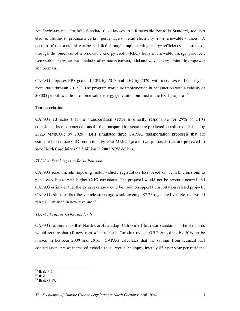
Transportation CAPAG estimates that the transportation sector is directly responsible for 29% of GHG
emissions. Its recommendations for the transportation sector are predicted to reduce emissions by
232.3 MMtCO2e by 2020. BHI simulated three CAPAG transportation proposals that are
estimated to reduce GHG emissions by 95.6 MMtCO2e and two proposals that are projected to
save North Carolinians $3.5 billion in 2005 NPV dollars.
TLU-3a: Surcharges to Raise Revenue CAPAG recommends imposing motor vehicle registration fees based on vehicle emissions to
penalize vehicles with higher GHG emissions. The proposal would not be revenue neutral and
CAPAG estimates that the extra revenue would be used to support transportation related projects.
CAPAG estimates that the vehicle surcharge would average $7.25 registered vehicle and would
raise $37 million in new revenue.28
TLU-5: Tailpipe GHG standards CAPAG recommends that North Carolina adopt California Clean Car standards. The standards
would require that all new cars sold in North Carolina reduce GHG emissions by 30%, to be
phased in between 2009 and 2016. CAPAG calculates that the savings from reduced fuel
consumption, net of increased vehicle costs, would be approximately $60 per year per resident.
26 Ibid, F-2. 27 Ibid. 28 Ibid, G-17.

The Economics of Climate Change Legislation in North Carolina/ April 2008 16
CAPAG translates this into a savings of $38 per ton of CO2e, for a net savings of $1.7 billion, in
net present value terms, for the period to year 2020.
TLU-6: Biofuels Bundle CAPAG proposal TLU-6 would increase the percentage of biofuel sales in the state’s gasoline
and diesel markets. Biofuels are produced from either a starch or cellulosic ethanol base,
procured from plants. CAPAG proposes several incentives, combined with a state government
mandate, to achieve its goals. CAPAG also proposes to eliminate the motor fuels tax on the
biofuel portion of gasoline and diesel and provide a $0.25 per gallon tax credit.29
CAPAG sets out a timeframe for replacing gasoline and diesel with biofuels. The first target is to
replace 10% of gasoline sales and 5% of diesel sales by 2010. CAPAG calls for the penetration
rate to rise 5% every five years until reaching 25% of gasoline sales and 20% of diesel sales by
2025.30 There would also be a cost trigger built into the system, where if the cost of alternative
fuel exceeds conventional fuel by more than a specified amount, the renewable fuel standard
would be suspended until the cost is back in the “acceptable” range.
ES-4: Cap and Trade A Cap and Trade system is a pseudo-market mechanism in which CO2 and other GHG emissions
are limited or capped at a specified level, and where those participating in the system can trade
permits (a permit is an allowance to emit one ton of CO2 or GHG). The permit allows emitters
either to reduce their emissions or to buy a permit to release GHG, whichever is less expensive.
The market for permits is created by government fiat and the value of the permits depends on the
number issued. Therefore, the number of permits issued or allocated is, in effect, the cap. The
cap can apply to single industrial sectors, such as manufacturing or electric utilities, a
combination of sectors or all sectors in the economy.
CAPAG recommends a Cap and Trade program applicable to North Carolina within the
framework of a national or regional plan. Although CAPAG provides estimates of the costs and
GHG reductions of such a program, it does not provide the details of a prospective regulatory
program.31
29 Ibid, G-30. 30 Ibid, G-29. 31 Ibid, F-22.

The Economics of Climate Change Legislation in North Carolina/ April 2008 17
BHI based its analysis of a Cap and Trade program for North Carolina on the national proposal
contained in America's Climate Security Act of 2007 (S. 2191).32 The Act includes the following
provisions:
• An emissions cap of 5,775 MMTCO2e by 2012, declining to 1,732 MMTCO2e by 2050;
• Permission to participate in allowance trading, borrowing and banking;
• A domestic offset program to sequester GHGs in agriculture and forests;
• A Carbon Market Efficiency Board to observe and report on the national GHG emission market and provide cost relief measures if it determines that the market poses significant harm to the U.S. economy;
• The distribution of emission allowances, including initially giving allowances to specified owners and operators of covered facilities, states and load-serving entities;
• The establishment of a Climate Change Credit Corporation to auction emission allowances; and
• The use of auction proceeds for zero- or low-carbon energy technologies programs.
The Act aims to reduce total U.S. greenhouse gas emissions to 70 percent below their 2005 levels
by the year 2050, utilizing a Cap and Trade system. The system would cover the electric power,
industrial petroleum based fuels and chemical sectors.
32 America's Climate Security Act of 2007, S 2191 110th Cong. 1st sess. http://www.govtrack.us/congress/bill.xpd?bill=s110-2191 (accessed April 17, 2008).

The Economics of Climate Change Legislation in North Carolina/ April 2008 18
BHI Estimates and Results Each of these proposals consists of either a tax or a fee added to the purchase of a product, such
as a vehicle surcharge, or seeks to increase the purchase and use of products such as biofuels that
emit fewer greenhouse gases. BHI used the NC-STAMP model to measure the changes to the
North Carolina economy that would take place as a result of the CAPAG recommendations. Each
estimate represents the change that would take place in the indicated variable against a “baseline”
assumption about the value that variable would take in the indicated year.
Energy Demand and Supply Table 5 presents the effects on selected economic indicators and on state and local government
funds attributable to the following policy changes:
Demand Side Management Programs – RCI-1;
Expanded Energy Efficiency Funds – RCI-2;
Public Benefits Charge – ES-7; and
Environmental Portfolio Standard – ES-2b.
The CAPAG recommendations for the energy sector would harm the North Carolina economy.
The private sector would shed 2,267 jobs in 2008, with losses increasing to 3,824 jobs by 2011.
The revenue raised from the public benefits charge would allow the public sector to add 936 jobs
in 2008, increasing to 1,351 by 2011. In total, the measures would extinguish an estimated 1,331
jobs in 2008 and 2,473 jobs by 2011, almost double the job losses under the policies proposed for
the transportation sector.
Although North Carolina would lose jobs, the wage rate would remain steady. North Carolinians
would face higher utility prices, which in turn would increase their cost of living. The cost of
living increase would, in turn, put upward pressure on households’ wage demands, since people
would need more money to cover their basic needs. The higher wage demands would add to the
already higher energy costs, leading producers to reduce their demand for labor, which would act
to temper the original increase in wage demands. These opposing forces balance out, with wages
remaining unchanged compared to the counterfactual.

The Economics of Climate Change Legislation in North Carolina/ April 2008 19
Table 5: Economic and Fiscal Impact of Energy Sector Recommendations 2008 2009 2010 2011 Total Employment (Jobs) (1,331) (1,628) (1,996) (2,473)
Private (Jobs) (2,267) (2,695) (3,202) (3,824) Government (Jobs) 936 1,067 1,206 1,351
Gross Wage Rate ($) - - - 0.23 Investment ($ millions) (44.50) (53.38) (63.95) (76.72) Nominal Personal Income ($ millions) (107.00) (131.50) (161.50) (199.50) Real Disposable Income ($millions) (146.50) (173.50) (205.00) (242.50) Real DI per Capita ($) (12.11) (13.96) (15.92) (17.99) Real Gross Domestic Product ($millions) (205.44) (248.17) (298.71) (360.27) State Funds ($ millions) 127.55 152.82 180.85 214.44
Sales and Use Tax 143.13 171.40 203.05 241.37 Corporate Income Tax (1.85) (2.14) (2.39) (2.71) Franchise Tax (2.25) (2.62) (3.03) (3.52) Motor fuel taxes (0.67) (0.80) (0.96) (1.18) Highway use tax (0.33) (0.40) (0.47) (0.55) Insurance taxes (0.21) (0.25) (0.30) (0.36) Motor vehicle fees (0.15) (0.18) (0.22) (0.27) Personal income tax (5.60) (6.90) (8.60) (11.02) Cigarette and tobacco taxes (0.12) (0.14) (0.16) (0.18) Alcohol taxes (0.12) (0.14) (0.17) (0.20) Inheritance tax (0.04) (0.05) (0.07) (0.10) Unemployment insurance tax (0.71) (0.83) (0.96) (1.11) Natural gas tax (1.28) (1.46) (1.68) (1.92) Other taxes (0.20) (0.23) (0.28) (0.33) Fees (2.09) (2.48) (2.94) (3.52)
Local Funds ($ millions) (25.89) (30.87) (36.79) (44.16) Local tax on residential property (1.19) (1.58) (2.14) (2.98) Local tax on business property (7.05) (8.43) (10.07) (12.04) Local sales and use taxes (8.90) (10.65) (12.62) (15.02) Local other taxes and fees (8.75) (10.22) (11.96) (14.12)
Total Funds ($ millions) 101.66 121.95 144.06 170.29 Figures are on Calendar Year Basis
The combination of higher energy prices and lower employment under the CAPAG proposals
would reduce incomes in North Carolina. Real disposable income would fall by $146.5 million
in 2008, sliding another $100 million, to reach a loss of $242.5 million in 2011.

The Economics of Climate Change Legislation in North Carolina/ April 2008 20
The higher cost of energy would hurt firms’ profit margins, causing them to reduce investment in
North Carolina. We estimate that investment in North Carolina would drop by $44.5 million in
2008 and $76.7 million in 2011, with the utility sector accounting for three-quarters of the
decrease by 2011.
The combination of lower investment, employment and incomes would shave $205.4 million off
of real GDP in North Carolina for 2008 and $360.3 million by 2011.
State government revenues increase due to the new public benefits charge and expanded energy
efficiency funds, which we treat as taxes on the utility sector. As a result, tax revenue would
increase by $143.1 million in 2008 and $241.4 million in 2011. The drop in employment and real
incomes would reduce other state tax revenues resulting in net state tax revenue gains of $127.6
million in 2008 and $214.4 million in 2011. The negative economic effects of the proposals also
reduce local tax revenues by $25.9 million in 2008 and by $44.2 million by 2011.
Transportation
Table 6 presents the changes in different economic indicators and in state and local government
funds, due to the following policy changes that affect the Transportation industry:
Vehicle Surcharge – TLU-3a
California Emissions Standard – TLU-5
Biofuels Bundle – TLU-6
The first economic indicator we consider is employment. The public sector would be able to
expand employment slightly due to the increase in the revenue from the higher vehicle fees, while
the number of jobs in the private sector would fall compared to baseline employment levels. This
would be caused by the increase in vehicle fees and the higher fuel and vehicle prices associated
with the adoption of the Biofuels Bundle program and the California Emissions Standards. We
estimate that North Carolina would employ 1,003 fewer people in 2008 and 1,202 in 2011 under
the plan.
Employment losses lead to a slight drop in annual wages – by $46 in 2008 and by $55 in 2011.
These decreases in wages and employment cause total personal income in the state to fall by $365
million in 2009 and by $469.5 million in 2011. The increase in vehicle surcharges, the decrease
The Economics of Climate Change Legislation in North Carolina/ April 2008 21
in total personal income and a rise in fuel and vehicle prices combine to reduce real disposable
income by $45 million in 2008 and by $46.5 million in 2011.
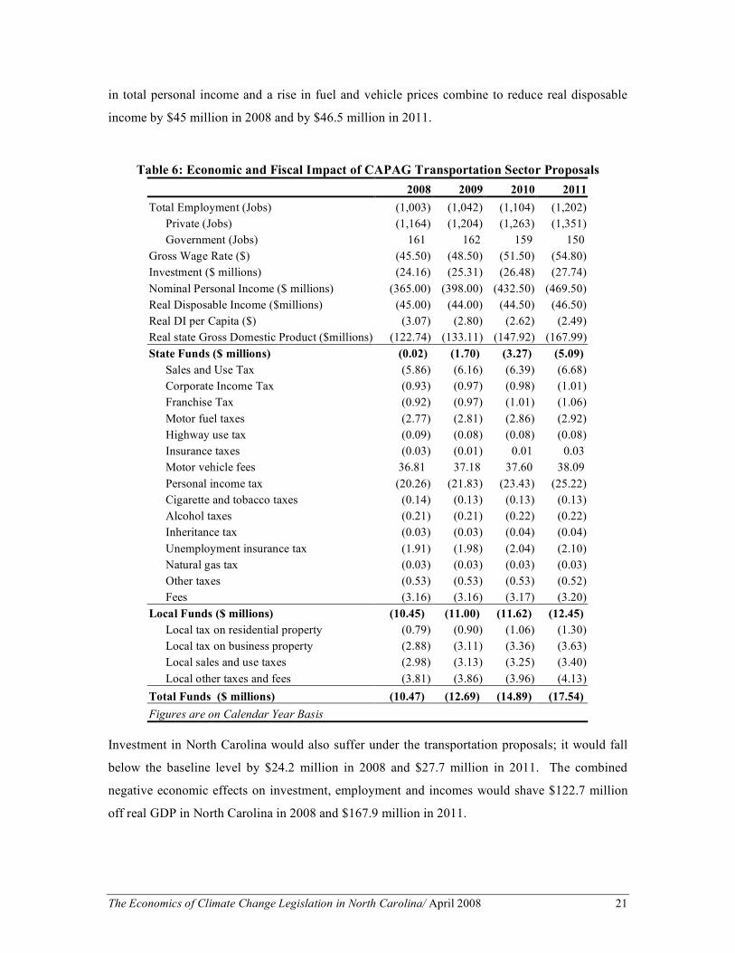
Table 6: Economic and Fiscal Impact of CAPAG Transportation Sector Proposals
2008 2009 2010 2011 Total Employment (Jobs) (1,003) (1,042) (1,104) (1,202)
Private (Jobs) (1,164) (1,204) (1,263) (1,351) Government (Jobs) 161 162 159 150
Gross Wage Rate ($) (45.50) (48.50) (51.50) (54.80) Investment ($ millions) (24.16) (25.31) (26.48) (27.74) Nominal Personal Income ($ millions) (365.00) (398.00) (432.50) (469.50) Real Disposable Income ($millions) (45.00) (44.00) (44.50) (46.50) Real DI per Capita ($) (3.07) (2.80) (2.62) (2.49) Real state Gross Domestic Product ($millions) (122.74) (133.11) (147.92) (167.99) State Funds ($ millions) (0.02) (1.70) (3.27) (5.09)
Sales and Use Tax (5.86) (6.16) (6.39) (6.68) Corporate Income Tax (0.93) (0.97) (0.98) (1.01) Franchise Tax (0.92) (0.97) (1.01) (1.06) Motor fuel taxes (2.77) (2.81) (2.86) (2.92) Highway use tax (0.09) (0.08) (0.08) (0.08) Insurance taxes (0.03) (0.01) 0.01 0.03 Motor vehicle fees 36.81 37.18 37.60 38.09 Personal income tax (20.26) (21.83) (23.43) (25.22) Cigarette and tobacco taxes (0.14) (0.13) (0.13) (0.13) Alcohol taxes (0.21) (0.21) (0.22) (0.22) Inheritance tax (0.03) (0.03) (0.04) (0.04) Unemployment insurance tax (1.91) (1.98) (2.04) (2.10) Natural gas tax (0.03) (0.03) (0.03) (0.03) Other taxes (0.53) (0.53) (0.53) (0.52) Fees (3.16) (3.16) (3.17) (3.20)
Local Funds ($ millions) (10.45) (11.00) (11.62) (12.45) Local tax on residential property (0.79) (0.90) (1.06) (1.30) Local tax on business property (2.88) (3.11) (3.36) (3.63) Local sales and use taxes (2.98) (3.13) (3.25) (3.40) Local other taxes and fees (3.81) (3.86) (3.96) (4.13)
Total Funds ($ millions) (10.47) (12.69) (14.89) (17.54) Figures are on Calendar Year Basis
Investment in North Carolina would also suffer under the transportation proposals; it would fall
below the baseline level by $24.2 million in 2008 and $27.7 million in 2011. The combined
negative economic effects on investment, employment and incomes would shave $122.7 million
off real GDP in North Carolina in 2008 and $167.9 million in 2011.
The Economics of Climate Change Legislation in North Carolina/ April 2008 22
The proposed transportation policies would hurt the North Carolina economy, but they also
encroach on the ability of state and local governments to provide goods and services. The
negative effect on income and employment shrink the state’s personal income tax collections by
$20.3 million in 2008 and $25.2 million in 2011 and the state’s sales tax revenue by $5.9 million
in 2008 and $6.7 million in 2011. These losses alone nearly cancel out the extra revenue
generated from the increase in the state’s motor vehicle fees. Local governments also would
suffer revenue losses under the proposals – $10.5 million in 2008, increasing to nearly $12.5
million in 2011.
Note that this loss in government revenue, at both the state and local levels, would not result from
a drop in the taxes paid by the individuals or businesses in North Carolina. After all, the vehicle
surcharge is really a fee increase. The damage to the economy brought about by the forced use of
more costly production methods, as well as the increase in the fees would translate into lower
revenues for other taxes, while also causing North Carolina residents to lose jobs and purchasing
power.
Cap and Trade
Table 7 presents the changes to the different economic indicators and to the state and local
governments’ funds caused by implementing a Cap and Trade system based on the Climate
Security Act of 2007.
The Cap and Trade system would produce the most damage to the North Carolina economy. The
economy would shed 24,640 jobs in 2008, with losses increasing to 29,808 jobs in 2011. The
private sector would absorb the brunt of the job loses, as energy and transportation price increases
push up the cost of doing business in the state. Some firms would react by cutting back on
production and subsequently payrolls; others would relocate to a lower cost (foreign) production
site; and yet others, no longer able to compete, would simply shut their doors. State and local
governments would not be immune to the price increases and, unless measures were made to
boost revenues, which would likely damage the North Carolina economy even further, they
would not be able to provide the same level of services as before, leading to job losses. State and
local government in North Carolina would need to reduce their payrolls by 2,185 in 2008 and
3,095 in 2011.

The Economics of Climate Change Legislation in North Carolina/ April 2008 23
Table 7: Economic and Fiscal Impact of Cap and Trade
2008 2009 2010 2011 Total Employment (Jobs) (24,640) (25,904) (27,552) (29,808)
Private (Jobs) (22,455) (23,514) (24,876) (26,713) Government (Jobs) (2,185) (2,390) (2,676) (3,095)
Gross Wage Rate ($) (215.50) (222.00) (227.00) (229.91) Investment ($ millions) (330.49) (351.10) (373.44) (397.93) Nominal Personal Income ($ millions) (2,259.50) (2,418.00) (2,598.50) (2,808.50) Real Disposable Income ($millions) (1,766.50) (1,826.50) (1,895.00) (1,976.50) Real Disposable Income per Capita ($) (131.82) (131.53) (130.47) (128.32) Real Gross Domestic Product ($ millions) (3,601.41) (3,711.59) (3,841.71) (4,002.64) State Funds ($ millions) (164.01) (175.93) (190.59) (211.47)
Sales and Use Tax 0.25 (0.33) (1.07) (2.05) Corporate Income Tax (13.89) (14.27) (14.12) (14.28) Franchise Tax (15.10) (15.60) (16.12) (16.68) Motor fuel taxes 9.63 9.27 8.72 7.80 Highway use tax (3.93) (4.05) (4.19) (4.35) Insurance taxes (2.56) (2.68) (2.82) (2.99) Motor vehicle fees 2.20 2.15 2.05 1.88 Personal income tax (113.74) (122.34) (133.39) (149.07) Cigarette and tobacco taxes (1.43) (1.44) (1.45) (1.46) Alcohol taxes (1.45) (1.50) (1.55) (1.62) Inheritance tax (0.72) (0.81) (0.94) (1.12) Unemployment insurance tax (10.25) (10.41) (10.60) (10.81) Natural gas tax 1.85 1.87 1.89 1.91 Other taxes (1.03) (1.09) (1.16) (1.25) Fees (13.85) (14.73) (15.86) (17.39)
Local Funds ($ millions) (90.67) (99.39) (110.72) (125.83) Local tax on residential property (21.60) (24.85) (29.38) (35.86) Local tax on business property (47.35) (50.28) (53.53) (57.02) Local sales and use taxes 0.13 (0.17) (0.55) (1.05) Local other taxes and fees (21.86) (24.10) (27.27) (31.91)
Total Funds ($ millions) (254.68) (275.32) (301.31) (337.30) Figures are on Calendar Year Basis
The higher cost of energy would hurt profit margins, causing firms to reduce investment in North
Carolina. We estimate that investment in North Carolina would drop by $330.5 million in 2008
and $397.9 million in 2011.
The job losses would result in sharply lower incomes for North Carolina residents. Annual gross
wages would drop by over $215.5 in 2008 and $229.9 by 2011, and real (price-adjusted)
disposable income would slump by $1.7 billion or $131.8 dollars per person in 2008 and $1.9

The Economics of Climate Change Legislation in North Carolina/ April 2008 24
billion, or $128.2 per person in 2011. The combined negative economic effects on investment,
employment and incomes would shave $3.6 billion off real GDP in North Carolina in 2008 and
$4 billion in 2011.

The Economics of Climate Change Legislation in North Carolina/ April 2008 25
Conclusion In its draft final report, CAPAG offered 56 recommendations for reducing GHG emissions
covering four sectors of the state economy. CAPAG mandates the use of less efficient and more
expensive renewable energy sources, public funding for untested programs to promote energy
efficiency and participation in a national or regional Cap and Trade program to limit GHG
emissions.
Contrary to CAPAG’s assertions, the implementation of these measures would not bring
“significant cost savings for the State’s economy” but would rather increase costs in the energy,
transportation and building sectors.33 The programs would raise the prices consumers and
businesses in North Carolina pay for energy, transportation and construction. It is, at the same
time, unlikely that these new programs would lead to improvements in efficiency that would
offset the increased prices at some undetermined date in the future. Meanwhile, the North
Carolina business community would see a reduction in its competitive advantage over other states
that resisted the pressure to adopt similar legislation. State GDP would be one percentage point
below baseline by 2011.
The North Carolina legislature should consider the CAPAG proposals in light of their likely
economic consequences. It should understand that, whatever the benefits of those proposals, they
will exert measurable, negative effects on the state economy. To assert that it is possible to adopt
sweeping greenhouse gas legislation without exerting such effects is to throw economic analysis,
as well as common sense, to the wind.
33 CAPAG, Draft Final Report, ES-2.

The Economics of Climate Change Legislation in North Carolina/ April 2008 26
Appendix A: Simulation Methodology
BHI simulated the implementation of eight CAPAG recommendations using NC-STAMP. Each
proposal was entered into the model as a change in the price of energy, or the introduction of a
tax, for an industrial sector, specifically, the utility or transportation sector. This appendix
contains a description of the methodology BHI used to estimate the price change or tax.
Energy Demand
RCI-1: Demand Side Management Programs BHI assumed the program would begin by allocating 0.5% of utility revenues in 2008, increasing
by 0.25% per year until reaching a maximum of 1.5% of revenues in 2011. BHI treats the
revenues as an excise tax levied on the utility sector. The revenues raised by this excise tax
would flow through a “Special Other” state government fund. From this fund, 25% of the
revenue is allocated to the general fund and distributed to all sectors in proportion to all other
general fund revenue. We assumed that this 25% would support staffing and other needs to
implement the program. The remaining 75% of the funds are allocated to the construction, real
estate, electrical equipment and professional, technical and scientific services sectors with equal
weighting.
RCI-2: Expand Energy Efficiency Funds In proposal RCI-2, CAPAG calls for a Public Benefit Charge (PBC) that is virtually identical to
the one proposed by ES-7 in the energy sector.
For modeling purposes, BHI assumes that these recommendations are separate and additive in
terms of their impact on utility prices. BHI increased the implicit excise tax on the utility sector –
also used to model ES-7 – by an additional 1% of industry revenues. The revenue was allocated
to the “Special Other” state fund and allocated to the construction, real estate, electrical
equipment and professional, technical and scientific services sectors using the same method as in
our treatment of RCI-1.

The Economics of Climate Change Legislation in North Carolina/ April 2008 27
ES-7 Public Benefits Charge
Since electricity usage in North Carolina is projected to continue to rise over the next few years,
the revenue from the PBC would also rise in line with electricity usage. BHI estimates that an
average PBC would raise $120 million in revenue by 2011. We treat the PBC as a new excise tax
on the utility sector and allocate the revenue to the Special Other fund in the North Carolina-
STAMP model simulations
Energy Supply
ES-2b: Environmental Portfolio Standard BHI utilized data from the Energy Information Administration of the U.S. Department of Energy
and results from a report by LaCapra Associates prepared for the North Carolina Utilities
Commission to estimate the effect the EPS would have on electricity prices.34 Using this
information, we estimate that prices for the North Carolina utility sector would increase by 0.44%
in 2008 and by 1.61% in 2011. We increased the price index for the utility sector in NC-STAMP
by these amounts against the counterfactual of no change in policy.
Transportation
TLU-5: Tailpipe GHG standards The CAPAG report cites three studies of the effects of tighter emission standards for new cars:
one shows huge cost savings; the second assumes that it would cost $1,000 to upgrade each
vehicle, but there would be net savings; and the third estimates that the upgrade would cost
$3,000 per vehicle, resulting in a situation where “savings on fuel would offset less than half of
that cost for consumers.”35 Following these estimates, “in an effort to be conservative,” CAPAG
opts for the results of the second study, and thus finds nearly $1.69 billion in net savings.36
BHI uses the mean of the cost estimates cited by CAPAG ($1,000 to $3,000) for the stricter
emissions standards, or $2,000 per new car. CAPAG cites a California Air Resources Board
estimate that fuel savings offset over 100% of their estimate of $1,000 in manufacturing cost 34 LaCarpa Associates, Analysis of a Renewable Portfolio Standard for the State of North Carolina (December, 2006): 61, http://www.ncuc.net/rps/rps.htm (accessed April 17, 2008). 35CAPAG, Draft Final Report, G-27. 36 Ibid, G-28.

The Economics of Climate Change Legislation in North Carolina/ April 2008 28
estimates, and a national automobile manufacturer’s estimate that the fuel savings would offset
less than half of the increased manufacturing costs. We assume that the fuel savings would
amount to half the manufacturing costs, or $1,000, resulting in net cost of $1,000 per new vehicle
sold in North Carolina.
Using U.S. Bureau of Transportation Statistics data for national new car sales and car registration
data for North Carolina, we calculate the ratio of vehicle registrations in North Carolina to total
registrations in the United States as 2.5%.37 We apply this ratio to total new car sales in the
United States, as reported by the U.S. Department of Commerce, to estimate the number of new
cars sold in North Carolina in 2005.38 We grow this figure by the average growth rate for new
cars in the U.S. from 1990 to 2004, or 1.3%, to estimate new car sales in North Carolina for 2008-
2011. We multiply the estimated increase in new car cost, $1,000 per car, by the new car sales to
estimate the total increase in new car costs at $449 million in 2008. This figure represents 3.04%
of the total transportation equipment manufacturing sector in the NC-STAMP model.
We increase the price index for the transportation equipment manufacturing sector by 3.04% in
the transportation simulation, against the counterfactual of no change, to estimate the impact of
TLU-5 on the North Carolina economy.
TLU-3a: Surcharges to Raise Revenue BHI uses the CAPAG estimates of increases in motor vehicle fees of $37 million in the NC-
STAMP model against the counterfactual of no increase. Since it is not clear from the CAPAG
report exactly how these funds are to be used, other than to support a reduction in vehicle miles
traveled, or the true effectiveness of the programs, we allocate the funds to the state highway and
highway trust funds.
TLU-6: Biofuels Bundle CAPAG provides no estimate of the costs or savings from the biofuels bundle recommendations.
BHI, however, has provided estimates through 2011. Ethanol is less expensive than gasoline or
diesel fuel on a per gallon basis, but ethanol produces less energy than gasoline and diesel. This 37 U.S. Department of Transportation, Bureau of Transportation Statistics, “State Transportation Statistics 2005,” in “Table 5-1: Motor-Vehicle Registrations,” http://www.bts.gov/publications/state_transportation_statistics/state_transportation_statistics_2005/index.html, (accessed April 17, 2008). 38 U.S. Department of Commerce, Bureau of Economic Analysis, “Underlying Detail for the National Income and Product Account Tables,” http://www.bea.doc.gov/, table 7.2.5S. (accessed April 17, 2008).

The Economics of Climate Change Legislation in North Carolina/ April 2008 29
lower energy concentration translates into a lower driving mileage per gallon for ethanol relative
to gasoline and diesel. As a result ethanol becomes more expensive to use than gasoline or diesel.
Since CAPAG does not specify the cost differential for the proposed “cost trigger” we assume no
cost trigger in our analysis.
Using data from the U.S. Bureau of Transportation Statistics (BTS) and the U.S. Energy
Information Agency (EIA), BHI estimates that reaching the percentages mandated in TLU-6
would add 1.16% to transportation costs over the period of 2008 to 2011.
We begin with the BTS estimate of motor fuel use for each state for 2005.39 We inflate this
figure through 2011 using the annual percentage change in the EIA estimate for U.S. energy
consumption for motor fuels.40 We then estimate the amount of ethanol consumption in North
Carolina for 2008-2011 by inflating the EIA estimate for 2005 by the estimated increase in U.S.
ethanol consumption for 2006 to 2011.41 The ethanol projection is subtracted from the gasoline
projection for each year, since the gasoline figure includes ethanol, according to a note in the EIA
table. We next calculated the total British Thermal Units (BTUs) that our predicted consumption
of gasoline and ethanol combined would produce for each year, using the BTU per gallon figures
from the EIA.42
We calculated the number of gallons of ethanol that would be consumed in North Carolina to
reach the percentage mandated by CAPAG. This is not straightforward, since every new gallon
of ethanol produces fewer BTUs than the gallon of gasoline it replaces. Thus, if we were simply
to replace gasoline, gallon for gallon, with ethanol, drivers would not be able to travel the same
distance as before. To complete the calculation we utilize the Microsoft EXCEL “solver” utility.
Solver allows us to compute the number of gallons of ethanol and gasoline that would satisfy the
39 U.S. Department of Transportation, Bureau of Transportation Statistics, “State Transportation Statistics 2006, in “Table 7-4: Motor Fuel Use: 2005,” http://www.bts.gov/publications/state_transportation_statistics/state_transportation_statistics_2006/html/table_07_04.html (accessed April 17, 2008). 40 U.S. Department of Energy; Energy Information Administration, “Energy Consumption by Sector and Source,” in “Table 2: Energy Price and Expenditure Estimates by Source, 1970-2005, North Carolina,” http://www.eia.doe.gov/oiaf/aeo/excel/aeotab_2.xls (accessed April 17, 2008). 41 U.S. Department of Energy; Energy Information Administration in “Table C4: Estimated Consumption of Alternative Fuels by State and Fuel Type, 2005,” http://www.eia.doe.gov/cneaf/alternate/page/atftables/afvtransfuel_II.html (accessed April 17, 2008). 42U.S. Department of Energy; Energy Information Administration, “Forecasts and Analysis, Alternative Fuels: Ethanol,” http://www.eia.doe.gov/oiaf/ethanol3.html. See also the calculator at “Energy Kids Page,” http://www.eia.doe.gov/kids/energyfacts/science/energy_calculator.html#mogascalc. (accessed April 17, 2008).

The Economics of Climate Change Legislation in North Carolina/ April 2008 30
CAPAG goal, while keeping the total number of BTUs generated from both unchanged from the
initial calculation. This calculation is performed for each year.
Finally, we calculated the dollar cost of the new mix of gasoline and ethanol consumption in
North Carolina. We used EIA projections for gasoline and ethanol prices to calculate the
difference between the cost of the original mix of gasoline and ethanol and the new mix, or $179
million.43 This represents 0.83% of the transportation sector spending in the NC-STAMP model.
The process was repeated to estimate the increase in costs under the diesel portion of the CAPAG
Biofuels Bundle proposal. We estimated that diesel fuel would increase costs by $5.6 million,
which represents 0.33% of the revenues of the transportation sector in the NC-STAMP model.
We increased the price index for the transportation sector in NC-STAMP by 1.16% (0.83 + 0.33)
against the counterfactual of no change in policy.
ES-4 Cap and Trade BHI modeled a Cap and Trade program for North Carolina based on the national proposal
contained in America's Climate Security Act of 2007 (S. 2191).44 The National Association of
Manufacturers (NAM) and the American Council for Capital Formation analyzed the Climate
Security Act using the National Energy Modeling System (NEMS). The NEMS model is used by
the U.S. Energy Information Administration (EIA) to respond to requests by Congress and federal
agencies for analyses of energy and environmental proposals. The NAM study reports national
and state specific results based on high and low cost assumptions, including changes in energy
and transportation fuel prices.45
BHI utilized the NEMS price change results for the U.S. and North Carolina to provide the basis
for the price change inputs to NC-STAMP. The NAM study assumes the Cap and Trade system
would become effective in 2011 and predicts U.S. price changes for the years 2014, 2020 and
2030.46 The study also reports estimates for North Carolina in 2020.47 The study presents the
43 U.S. Department of Energy; Energy Information Administration, Annual Energy Outlook: 2008 (Early Release) in “Table 3. Energy Prices by Sector and Source,” http://www.eia.doe.gov/oiaf/aeo/excel/aeotab_3.xls (accessed April 17, 2008). 44 America's Climate Security Act of 2007, S 2191, 110th Cong. 1st sess., GovTrack.us, http://www.govtrack.us/congress/bill.xpd?bill=s110-2191 (accessed April 17, 2008). 45 American Council for Capital Formation and National Association of Manufacturers, Analysis of Lieberman-Warner Climate Security Act (S. 2191) Using the National Energy Modeling System (March 13, 2008) Internet; http://www.accf.org/pdf/NAM/fullstudy031208.pdf (accessed April 17, 2008). 46 Ibid, 8.

The Economics of Climate Change Legislation in North Carolina/ April 2008 31
price changes for gasoline, residential and industrial electricity, natural gas and coal fired
electricity under the low and high cost scenarios against the baseline. They also report changes in
overall energy expenditures for 2012 and 2014.
BHI calculated the ratio of the 2020 prices changes in North Carolina to the prices changes in the
United States for each category of energy listed above. This ratio was used to adjust the 2014
prices reported for the United States to approximate North Carolina price changes in 2014.
BHI used 2005 North Carolina energy expenditures by their commodity source (coal, natural gas,
gasoline, retail electricity), as reported by the Energy Information Agency of the U.S. Department
of Energy, to determine the percentage of energy expenditures by source to the total energy
expenditures for the four categories.48 The percentages were used to allocate the price changes
for each source of energy, as reported by NAM, to the total change for the North Carolina energy
sector. The result for each category was summed to arrive at an adjusted 2014 price change for
the energy sector.
We obtained the estimated price change for 2012 by using the ratio of 2012 to 2014 national
prices, as reported by NAM. Using this methodology, we estimated that the energy price would
increase by 11.4% in the first year of Cap and Trade. On the basis of this calculation, we
increased the price index for the utility sector by 11.4% in NC-STAMP and ran the simulation
against the counterfactual of no change.
We estimated the transportation sector price increase resulting from the implementation of a Cap
and Trade system using a similar method as above. We first calculated the average U.S. gasoline
price increase reported by NAM. The U.S. price increase for gasoline in 2014 was adjusted to
North Carolina using the difference between the North Carolina and U.S. prices increase reported
for the year 2020.
We calculated the ratio of gasoline expenditures to total transportation expenditures for North
Carolina. This percentage was multiplied by the percentage increase in North Carolina gasoline
price to obtain the total estimated increase in transportation prices under Cap and Trade, or 7.8%,
47 See ACCF and NAM, “North Carolina: Economic Impact on the State from the Lieberman-Warner Proposed Legislation to Reduce Greenhouse Gas Emissions,” from Analysis http://www.accf.org/pdf/NAM/NorthCarolina.pdf (accessed April 17, 2008). 48 U.S. Department of Energy; Energy Information Administration, in “Table 1: Energy Price and Expenditure Estimates by Source, 1970-2005, North Carolina,” http://www.eia.doe.gov/states/sep_prices/total/pr_tot_nc.html (accessed April 17, 2008).

The Economics of Climate Change Legislation in North Carolina/ April 2008 32
for the first year. We increased the price index for the transportation sector by 7.8% in the NC-
STAMP model and ran the simulation against the counterfactual of no change.

The Economics of Climate Change Legislation in North Carolina/ April 2008 33
Appendix B: NC-STAMP
NC-STAMP is a comprehensive model of the North Carolina economy, designed to capture the
principal effects of city and state tax changes on that economy. NC-STAMP is a five-year
dynamic Computable General Equilibrium (CGE) tax model. As such, it provides a mathematical
description of the economic relationships among producers, households, government and the rest
of the world. It is general in the sense that it takes all the important markets and flows into
account. Because it assumes that demand equals supply in every market (goods, services, labor
and capital), STAMP is an equilibrium model. It reaches equilibrium by allowing prices to adjust
within the model. With the help of a computer, the model is able to generate numeric solutions to
concrete policy and tax changes. It is, in particular, a tax model because it pays detailed attention
to identifying the role played by different taxes or equivalent price changes.49
We begin by distinguishing between producers and consumers. Consumers/households earn
income by supplying labor (wages and salaries) and capital (dividends and interest). Some of
these consumers also receive transfer payments such as pensions from the government.
Consumers maximize their discounted utility, which they get from consumption and leisure.
Their spending decisions are strongly influenced by the structure of prices they face; and the
amount of labor that they are willing to provide depends to a substantial degree on the wage rates
before them, as well as the taxes they have to pay.
Producers/firms buy inputs (labor, capital and intermediate goods that are produced by other
firms) and transform them into outputs. Producers maximize profits and are likely to change their
decisions about how much to buy or produce depending on the prices they face for inputs and
outputs.
In addition, there is a government sector that collects taxes and fees and provides services and
transfers. The rest-of-the world sector consists of the entire world outside of North Carolina. The
relationships between these components are set out in the circular flow diagram shown in Figure
1.50 The arrows in the diagram represent flows of money (for instance, households purchase
49 Shoven and Whalley, “Applied General-Equilibrium Models.” 50 Based on a similar diagram in Peter Berck, Elise Golan, and B. Smith with John Barnhart and Andrew Dabalen. “Dynamic Revenue Analysis for California.” University of California at Berkeley and California Department of Finance (1996): 117, http://www.dof.ca.gov.

The Economics of Climate Change Legislation in North Carolina/ April 2008 34
goods and services), and flows of goods and services (for instance, households supply their labor
to firms). The separate box for government shows the flows of funds to government in the form
of taxes, as well as government purchases of goods and services and government hiring of labor
and capital.
Figure 1. Circular Flow Diagram
Complex as it may seem, the diagram in Figure 1 is still too simple, because it lumps all
households into one group, and all firms into another. To provide further detail it is necessary to
create sectors; NC-STAMP has 81 economic sectors. Each sector is an aggregate that pulls
together segments of the economy. We separate households into seven income classes and firms
into 27 industrial sectors. In addition, we distinguish between 30 types of taxes and funds (four at
the federal level, 13 at the state level, and 12 at the city level) and 13 categories of government
spending (two at the federal level, six at the state level, and five at the city level). To complete
the model, there are two factor sectors (labor, capital), an investment sector and a sector that
represents the rest of the world. The availability of suitably disaggregated data (for households
and firms) as well as the particular state and city taxes and funds, dictate the choice of sectors.

The Economics of Climate Change Legislation in North Carolina/ April 2008 35
Sub-national models, such as NC-STAMP, are similar in many ways to national and international
CGE models. However, they differ in a number of important respects. Specifically:
a. In a national model, most saving goes toward domestic investment; however, this need
not be true at the regional level. If citizens of North Carolina save more than they spend,
then the excess saving will leak out of the state.
b. The smaller the unit under consideration, the greater the importance of trade with the rest
of the world. This is an important consideration for state models.
c. Migration is likely to be larger ─ and more responsive ─ across cities and states than
across nations.
d. In sub-national models, taxes are interdependent. So, for instance, the amount of revenue
collected by the Federal personal income tax depends significantly on whether there is a
state or local income tax (which may be deducted from income before computing the
Federal tax).
e. Data are less available at the sub-national than national level. This explains why scores
of national CGE models have been built, but relatively few sub-national models.
Constructing a CGE model
The construction of a CGE model involves several steps. First, one needs to organize the data
needed by the model. NC-STAMP starts with data for a single fiscal year, 2006, which we use as
a basis to develop a steady state path in the model through fiscal year 2011. This steady state path
is attained by applying growth rates for investment, population, employment and inflation
throughout the time frame of the model. In NC-STAMP, the investment growth rate is assumed
to be 1.31%.51 The growth rate for population is assumed to be 1.7%.52 The inflation growth rate
is assumed to be 3.00%53. To attain a reasonable steady state path, the data for the base year,
fiscal year 2006, must be very detailed. Most of the data are organized into a Social Accounting
Matrix (SAM), which in this case consists of an 81 by 81 matrix that accounts for the main
economic and fiscal flows in the state.
51 This figure is derived from taking the average nominal US gross domestic investment for the period 1929-2004 as published by the Bureau of Economic Analysis. 52 This figure is the Census projection for North Carolina for the period 2005-2010. 53 This figure is based on data obtained from the U.S. Bureau of Labor Statistics.

The Economics of Climate Change Legislation in North Carolina/ April 2008 36
The model also requires some additional information – for instance, data on employment and on
the structure of the Federal income tax – which are put in separate files. And the model requires
information on “elasticities;” these are the parameters, taken from the academic literature, that
measure the responsiveness of the different agents in the economy to changes in prices and costs.
These are set out in detail in Section 4 of this appendix. The economy is assumed to be
competitive, and to run at full employment (by which we mean that there is no involuntary
unemployment).
Second, the model needs to be specified in detail; the next section of this appendix sets out details
of the model that we constructed for North Carolina, along with some comments explaining the
choices made at each step.
The third step is to program the model. For this we used the specialized GAMS (General
Algebraic Modeling System) software. Before use, the model must be calibrated. We calibrate
the model under the assumption that the data gathered for the first year, 2006, represents the
optimal levels of the different variables for that year and, as mentioned earlier, using elasticities
from the literature. We know the model is correctly calibrated if, and only if, when it is run for
the first year, it replicates the values for all the variables that we had in our data. Calibration is a
crucial step in modeling the economy under consideration for obvious reasons.
The fourth step is to then open the model for growth into future years and solve the model.
Although this step may seem trivial, it is one of the most time consuming ones, since we check
for both consistency of publicly available data and the results the model returns. Once the model
solves for the five year period it considers, we run some counterfactuals to check on how well it
captures the changes in the variables that are considered in the model.
After making sure that the model solves for all its years, and that it returns consistent results, it is
ready for policy analysis. To allow for an easier use of the model, we develop a client interface
in Excel, where any user can change a tax rate or a level of revenue to be collected from
particular taxes, and can then use the internet to get the changes that those policy changes would
make in the economy. For the analysis in this report, however, specific programming was needed
to simulate the different changes mentioned. It is very important to note that NC - STAMP is a
policy model and not a forecasting model; in other words it is designed to answer “what if?”
questions, not to provide economic forecasts.
The Economics of Climate Change Legislation in North Carolina/ April 2008 37
Organizing the Data
The starting point in building a CGE model is to determine the degree of detail that is desired and
to organize the collected data into the useful format of a Social Accounting Matrix (SAM) for the
base year. The SAM that we developed for North Carolina is an 81 by 81 matrix. Each of the
5,929 cells in the matrix represents the dollar value of a flow from one sector of the economy to
another – for instance, purchases of business services by the utilities sector, or labor earnings
flowing to middle-income households. Reading along a row, one finds the payments received by
that sector; reading down a column, one sees the payments made by that sector. The SAM is
balanced, which means that the sum of the entries in any given row equals the sum of the entries
in the corresponding column. Thus, for instance, the revenue received by utilities must equal
spending by that sector, so that all incoming and outgoing funds are completely accounted for.
For NC-STAMP, we distinguish 27 industrial sectors, two factors (labor and capital), seven
household categories, an investment sector, 41 government sectors (23 for taxes, 13 for spending,
five government funds) and a sector for the rest of the world. In sectoring the economy we
sought to strike a balance between providing a high level of detail (especially on the tax side) and
keeping the model to a manageable size. An additional limitation is that the lack of finely
disaggregated data limits the degree of detail that is possible. Data availability also determined
some of the choices we made; for instance, it is possible to get a breakdown of households into
seven income categories (see below for further details), and while we might have preferred a
different set of categories, we were constrained by the nature of the data available.
Industrial sectors
Although data for 49 sectors were actually available from the Bureau of Economic Analysis, NC-
STAMP contains only 27 industrial sectors since some sectors were too small to merit separate
attention. In these cases, we combined some industries, such as textiles and apparel. In other
cases, there were no matching employment figures, and so it was easier to work with aggregates.
Factor Sectors We distinguish between two factors, labor and capital (the latter which includes land).
Businesses pay wages and salaries to labor, and rent on the capital they use to the capital owners.

The Economics of Climate Change Legislation in North Carolina/ April 2008 38
Since the model does not allow firms to have profits, as it assumes perfect competition general
equilibrium, the payments to capital include the redistribution of any earnings that companies
have.
Household Sectors
In NC-STAMP, households receive wages, capital income and transfers and they use this income
to buy goods and services, to pay taxes and fees and to save. We distinguish seven household
sectors, which group households by their levels of income. Expenditure data are available for
households in each of these categories, which make it relatively straightforward to work with this
structure. One purpose of this disaggregation of households is to allow one to trace the
distributive effect of tax changes and another one is to allow different groups to have different
levels of sensitivity to labor market conditions.
Investment Sector
There is one investment/savings sector. Both households and the government save and invest.
Information is available from the Bureau of Economic Analysis (BEA) on the pattern of gross
investment by destination (i.e., how much gross investment went into adding to the stock of
capital in utilities, in industry, and so on). We have constructed measures of the capital stock in
each sector, and by applying published depreciation rates and adding gross investment, arrived at
the capital stock in the subsequent period. This permits the model to track the expansion of the
economy over time. The BEA also produces a matrix, built for the U.S. for 1997, which maps
investment by destination with investment by source. This mapping allows one to determine, for
example, how much of the investment destined for utilities is spent on purchasing goods and
services from the construction sector and the transport sector. Thus if investment rises, it is
possible to identify which sectors would face an expansion in the demand for their output.
Government Sectors
NC-STAMP was designed primarily to analyze the effects of major changes in the structure of
state taxes, so we have paid particular attention to providing sufficient detail for government
transactions. The sectoring is summarized below in Table 8.

The Economics of Climate Change Legislation in North Carolina/ April 2008 39
The North Carolina government collects revenue from taxes and fees. Specific tax categories at
the state level included in the model are: sales and use, cigarettes and tobacco, motor fuels,
alcohol, inheritance, insurance, corporate and personal incomes. The rest of the state taxes are
grouped into a residual category (other local taxes).
The revenues from the taxes go to either the NC general fund, the NC capital projects fund or to
other funds, or a combination of them. Funds then allocate the money into the five spending
categories: education, health and welfare, transportation, public safety or others.
Table 8: Government Sectors Federal Government Receipts USSSTX Social Security (OASDI and
MEDICARE) Receives payments from employers and households; pays out transfers to households.
USPITX Federal Personal Income Tax Receives payments from households, which are put into the Federal normal spending account.
USCITX Federal Corporation Income Tax Receives payments from corporations and channels them into the Federal normal spending account.
USOTTX Other Federal Taxes Includes excises on motor fuel, alcohol, and tobacco; estate and gift taxes. Also funneled into the Federal normal spending account.
Federal Government Expenditure USNOND Federal Normal Spending Federal government purchases goods and
services, hires labor, and transfers money to NC and to Federal defense fund.
USDEFF Federal Defense Spending Purchases goods and services, and pays labor for military purposes.
NC State Government Receipts
STPITX State Personal Income Tax Revenues go into NC State general fund and other fund.
STSATX State Sales and Use Tax Revenues go into NC State general fund and other fund.
STCITX State Corporate Income Tax Revenues go into NC State general fund and other fund.
STIHTX North Carolina State Inheritance Tax Revenues go into NC State general fund.
STINTX North Carolina State Insurance Tax Revenues go into NC State general fund and other fund.
STFUTX State Taxes on Motor Fuels Revenues go into NC State Highway trust fund and highway fund.
STFRTX State Franchise Tax Revenues go into NC State general fund.
STHUTX State Highway Use Tax Revenues go into NC State highway trust fund.
STNGTX State Natural Gas Tax Revenues go into NC State general fund.
STALTX State Alcohol Beverage Taxes Revenues go into NC State general fund and other fund.
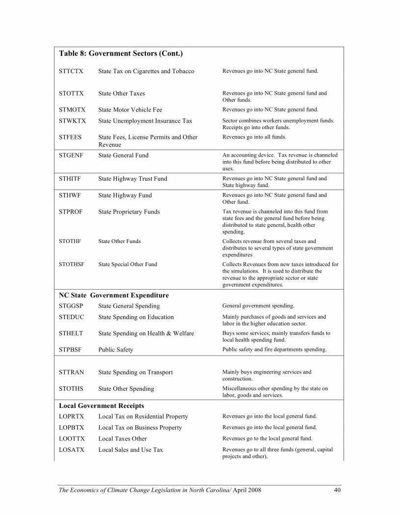
The Economics of Climate Change Legislation in North Carolina/ April 2008 40
Table 8: Government Sectors (Cont.)
STTCTX State Tax on Cigarettes and Tobacco Revenues go into NC State general fund.
STOTTX State Other Taxes Revenues go into NC State general fund and Other funds.
STMOTX State Motor Vehicle Fee Revenues go into NC State general fund.
STWKTX State Unemployment Insurance Tax Sector combines workers unemployment funds. Receipts go into other funds.
STFEES State Fees, License Permits and Other Revenue
Revenues go into all funds.
STGENF State General Fund An accounting device. Tax revenue is channeled into this fund before being distributed to other uses.
STHITF State Highway Trust Fund Revenues go into NC State general fund and State highway fund.
STHWF State Highway Fund Revenues go into NC State general fund and Other fund.
STPROF State Proprietary Funds Tax revenue is channeled into this fund from state fees and the general fund before being distributed to state general, health other spending.
STOTHF State Other Funds Collects revenue from several taxes and distributes to several types of state government expenditures
STOTHSF State Special Other Fund Collects Revenues from new taxes introduced for the simulations. It is used to distribute the revenue to the appropriate sector or state government expenditures.
NC State Government Expenditure STGGSP State General Spending General government spending.
STEDUC State Spending on Education Mainly purchases of goods and services and labor in the higher education sector.
STHELT State Spending on Health & Welfare Buys some services; mainly transfers funds to local health spending fund.
STPBSF Public Safety Public safety and fire departments spending.
STTRAN State Spending on Transport Mainly buys engineering services and construction.
STOTHS State Other Spending Miscellaneous other spending by the state on labor, goods and services.
Local Government Receipts LOPRTX Local Tax on Residential Property Revenues go into the local general fund.
LOPBTX Local Tax on Business Property Revenues go into the local general fund.
LOOTTX Local Taxes Other Revenues go to the local general fund.
LOSATX Local Sales and Use Tax Revenues go to all three funds (general, capital projects and other).

The Economics of Climate Change Legislation in North Carolina/ April 2008 41
Table 8: Government Sectors (Cont.) Local Government Expenditure LOEDUC Local Spending on Education Purchases goods and services and (mainly) pays
teacher salaries.
LOHELT Local Spending on Health & Welfare Purchases goods and services and pays labor; large transfers to the poorest category of households.
LOPBSF Local Public Safety Public safety and fire departments local spending.
LOTRAN Local Spending on Local Transportation Mainly buys engineering services and construction.
LOOTHS Local Other Spending Includes spending on police and firefighters, road repair, and miscellaneous local government services.
Rest of the World To complete the model, we have included a sector for the rest of the world (ROWSCT). This
refers to the world outside of North Carolina, i.e., the rest of the United States and other
countries. Information on flows between North Carolina and the rest of the world is difficult to
piece together, and is an area where considerable professional judgment was required.
NC-STAMP Equations NC-STAMP is a dynamic CGE model which assumes a steady state growth path. Absent from
any “shocks”, the economy is assumed to remain on this path. If the economy experiences a
shock, such as a tax change, the economy will diverge from this steady state path and eventually
turn onto a new path. The size and length of the divergence will depend on the size of the shock
to the economy. Below we set out the equations used in NC-STAMP and the assumptions
inherent in them.
Household Demand
Households are assumed to maximize their well being (“utility”) by picking baskets of goods and
services, subject to their budget constraints. The key set of equations in this section is labeled
Private Consumption, and consists of a set of demand functions. These demand functions, based
on a Cobb-Douglas utility function, take on the simple form,
,
,
* , 1,..., ; 1,...t
t i i
t i
IX i n t n
P!= = = ,

The Economics of Climate Change Legislation in North Carolina/ April 2008 42
where Xt,i is the quantity demanded of good i at time t, Pt,i is the price of good i at time t, It is
income at time t, and λi are parameters that measure the share of income that is devoted to good i.
This is the simplest specification that is theoretically satisfactory: it is additive (so spending
equals income less taxes less saving), has downward-sloping demand (ensuring that when the
price of a good rises, the quantity demanded falls), is zero degree homogeneous in prices and
income (so that if prices and incomes were to double, the quantity demanded would not change),
and meets the technical requirement of symmetry of the Slutsky matrix. More complex
formulations are possible, but there is a lack of reliable data on the elasticity parameters that
would be needed in such cases.
Household Gross Factor Income
Comments: The gross income of households in each of the seven groups (indexed by h in the
set H) is found by first summing factor income (yf) from labor and capital,
subtracting the social security contributions paid by employees, and then
allocating the total to each group on the basis of fixed shares. Factor payments
are allocated to each household group using the same fixed shares as were found
in the base year.
Eq. 1. ( ) FfHhTtFFPya
ay
Ff GFg
fh
fgtfft
Hh
w
htfh
w
htfh
ht !!!"##$
%&&'
())= * *
*! !
!
,,11,,,
,,
,,
,+
,
,
Description: Household income is the sum of income from each factor (labor and capital) less
factor taxes, distributed by household groups according to their share of total.
Data: The information on earnings for each household group comes from NC (North
Carolina) IMPLAN (an economic impact modeling system which allows users to
perform in-depth regional analysis. See http://www.implan.com for more
details).
Household Disposable Income

The Economics of Climate Change Legislation in North Carolina/ April 2008 43
Comments: Disposable household income is gross income, less taxes on household income
and property (mainly personal income tax (USPITX, STPITX) and residential
property tax (LOPRTX)), plus transfer payments (such as social security and
unemployment benefits).
Eq. 2. , , , , , , , , , , ,
,d hh h hh n pc
t h t h t g h t h t g h t h hg t h t h g
g GI g GH g G
y y t a a w a h H t T! !" " "
= # # + $ " "% % %
Description: Disposable household income is the household income less income taxes and
other household taxes (property taxes etc), plus the government transfer
payments.
Private Consumption Expenditure
Comments: This is the simplest demand system that is consistent with theoretical first
principles, and it requires only a limited number of parameters.
Eq. 3. TtHhIip
p
p
p
y
ycc
ii
ih
Ii
GSg
q
igt
GSg
c
igt
it
it
ht
ht
d
ht
d
ht
hithit !!!"
#####
$
%
&&&&&
'
(
))*
+,,-
.+
))*
+,,-
.+
))
*
+
,,
-
.÷= /
0
0
!
!
!,,
1
1
'
'
',,
',,
',
',
,
,
,
,
,,,,
1
2
3
3
Description: Consumption is a function of baseline consumption, adjusted to reflect the
change in household disposable income (in constant prices), and the change in
after-tax prices.
Data: By construction, this equation has zero cross price elasticities. In the absence of
adequate estimates of demand elasticities we follow the approach taken by Berck
et al., setting all income and own-price elasticities equal to unity.
Direct Household Purchases of Imports

The Economics of Climate Change Legislation in North Carolina/ April 2008 44
Comments: Some household spending goes directly to buy goods and services outside North
Carolina.
Eq. 4. , ,
, ,
,,
,
mh
d
t h t h
t h t h dt ht h
y pm m h H t T
py
!" #$ %= ÷ & ' '$ %( )
Description: Household imports will increase with the increase in disposable income, in
constant prices.
Household Savings
Comments: In NC-STAMP, household savings is the residual after spending and taxes have
been subtracted from income. Thus savings are seen as occurring passively.
Eq. 5. , , , , , , , ,
1 - ,d c
t h t h t i h t i t g i t h
i I g GS
s y c p m h H t T!" "
# $= % + & " "' (
) *+ +
Description: See comments above.
Data: The savings rates for households at each income level were adjusted based on
professional judgement, to account for the imputed savings by corporations
(which indirectly represents savings by the owners of the corporations).
Consumer Price Index
Comments: The price index in the reference period is set equal to 1. There is a separate price
index for each household group. This allows one to compute the real (rather than
nominal) income for each household group. For instance, a tax on foodstuffs
would tend to hit poor households relatively hard, and the CPI for poor
households would pick up this effect.

The Economics of Climate Change Legislation in North Carolina/ April 2008 45
Eq. 6. , , , , ,
,
, , , , ,
1
,
1
c
t i t g i t i h
i I g GS
t h
q
t i t g i t i h
i I g GS
p c
p h H t T
p c
!
!
" "
" "
# $+% &
' (= ) " "
# $+% &
' (
* *
* *
Description: Price index by household group is a function of the baseline price index, adjusted
by the change in after-tax prices by industry, according to their corresponding
share of consumption.
Data: The consumption of each good by each household group (cih) is derived from
reports published by State and Federal agencies. The model also generates some
of its own values.
Labor Supply
Comments: In NC-STAMP we model the labor participation rate, defined as the proportion
of households in any given income category that work. The participation rate is
assumed to rise if wage rates rise, if the taxes levied on earnings fall, or if the
transfer payments paid out per non-working household fall. The participation
rate for low-income households is assumed to be highly sensitive to the level of
transfer payments, but relatively insensitive to changes in taxes or the wage rate.
On the other hand, high-income households are assumed to respond substantially
to changes in the taxes and wage rates they face.
Eq. 7.
,
, ,1/
, ,, , , , ,
, ,
, ,, , , , , ,
,
,
tph
PITlsh gh
t h gGINUM
pihh ag Gt g ht h t L t h t h t hw w
t h t h hh a pit h gg GIt h t L t h t g h t h
g G t h
w
ta r p p pa a
wa r p t p
p
t T h H
!
!!
"
"
"
# $% &' (# $# $ % &) *= ÷ ÷% &% &% & % & % &) *+ , + ,- . % &+ ,
/ " "
01
0
Description: The supply of labor is a function of the baseline supply of labor adjusted by
population growth, the net change in wages, income taxes, and government
transfer payments. We used professional judgment in determining the proper
elasticities for each household group.
Data: The data on working households by income class came from IMPLAN.

The Economics of Climate Change Legislation in North Carolina/ April 2008 46
Population
Comments: The number of households in each income group depends first and foremost on
the initial number of households. To this we add the natural growth of the
population and net in-migration. Migration in turn depends on the level of after-
tax income, and the proportion of households that are not working (which reflects
the employment prospects facing new migrants). This formulation is in the spirit
of the migration model popularized by Harris and Todaro.54
Eq. 8.
, , , , ,
, , ,
, , , , ,
, , , , ,
, , , , ,
,
yd uhh
yd uhh
d d n n
t h t h t h t h t hhh hh i
t h t h t h hh hh hh hh
t h t h t h t h t h
d d n n
t h t h t h t h t ho
h hh hh hh hh
t h t h t h t h t h
y y p a aa a a
a a p a a
y y p a aa h
a a p a a
! !
! !
" # " #= + ÷ ÷ ÷$ % $ %$ % $ %
& ' & '
" # " #( ÷ ÷ ÷ ) *$ % $ %$ % $ %
& ' & ', H t T*
Description: See comments above.
Data: The elasticities used in this equation are the same as those used for California by
Berck et al. and “reflect the middle ground found in the literature about
migration.”55
Number of Non-Working Households
Comments: This is a simple accounting equation; the number of non-working households is
the total number of households, less the number that are working.
Eq. 9. , , ,
,n hh w
t h t h t ha a a h H t T= ! " # #
Description: See comments above.
54 John R. Harris and Michael P. Todaro, “Migration, Unemployment and Development: A Two Sector Analysis,” American Economic Review 40 (1970): 126-42. 55 Berck, et. al. “Dynamic Revenue Analysis.” See footnote 50.

The Economics of Climate Change Legislation in North Carolina/ April 2008 47
The Behavior of Producers/Firms
Producers are assumed to maximize profit. Combining intermediate inputs with labor and capital
produces output. The amount of intermediate inputs required per unit of output is fixed, but firms
have considerable leeway to vary the amounts of capital and labor that they use in production.
The value of output less intermediate inputs is value added, and it is useful to compute a price for
this value added; it is this price that determines factor demand – i.e. drives firms to hire more or
less labor and capital. The amounts of labor and capital inputs, in turn, drive the total value of
output via the production function.
Intermediate Demand
Comments: Intermediate goods constitute a fixed share of the value of production.
Eq. 10. , , , ,
,t i t i i t i
i I
v = q i I t T! " ""#
$ # #%
Description: See comments above.
Data: From the NC input-output table, derived from data from IMPLAN, which in turn
are based on data from by the Bureau of Economic Analysis.
Production Function
Comments: Output is determined by the quantities of labor and capital used in production; it
is assumed that enough intermediate goods will be available. We use a Constant
Elasticity of Substitution (CES) production function, which allows a degree of
substitution between labor and capital; in other words, if the price of labor rises,
firms will cut back on the number of workers they hire, and use more capital
instead.
Eq. 11. ( ) ( )-1
, , , , , , , ,
ii id
t i t i t f i t f i t i t
f F
q u g gk i I t T!
! !" # #
$ $
%
& '= + ( % %) *
+ ,-
Description: In addition to labor and capital used in production, we account for infrastructure.
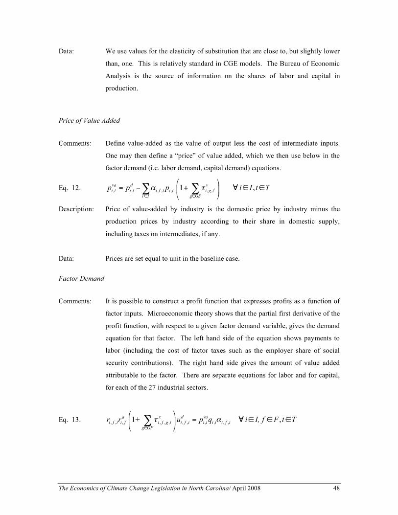
The Economics of Climate Change Legislation in North Carolina/ April 2008 48
Data: We use values for the elasticity of substitution that are close to, but slightly lower
than, one. This is relatively standard in CGE models. The Bureau of Economic
Analysis is the source of information on the shares of labor and capital in
production.
Price of Value Added
Comments: Define value-added as the value of output less the cost of intermediate inputs.
One may then define a “price” of value added, which we then use below in the
factor demand (i.e. labor demand, capital demand) equations.
Eq. 12. , , , , , , ,
1 ,va d v
t i t i t i i t i t g i
i I g GS
p p p i I t T! "# # ##$ $
% &= ' + ( $ $) *
+ ,- -
Description: Price of value-added by industry is the domestic price by industry minus the
production prices by industry according to their share in domestic supply,
including taxes on intermediates, if any.
Data: Prices are set equal to unit in the baseline case.
Factor Demand
Comments: It is possible to construct a profit function that expresses profits as a function of
factor inputs. Microeconomic theory shows that the partial first derivative of the
profit function, with respect to a given factor demand variable, gives the demand
equation for that factor. The left hand side of the equation shows payments to
labor (including the cost of factor taxes such as the employer share of social
security contributions). The right hand side gives the amount of value added
attributable to the factor. There are separate equations for labor and for capital,
for each of the 27 industrial sectors.
Eq. 13. , , , , , , , , , , , ,
1 ,a x d va
t f i t f t f g i t f i t i t i t f i
g GF
r r + u p q i I, f F t T! "#
$ %= & # # #' (
) *+

The Economics of Climate Change Legislation in North Carolina/ April 2008 49
Description: The factor demand at the current intra-industry rental rate (for labor and capital)
times the overall rental rate, including factor taxes is a function of the price of
value-added times the industry domestic supply.
Data: Information on the wage bills comes from the Bureau of Economic Analysis.
The total wage bill is divided by the number of workers (from the Bureau of
Labor Statistics) to get measures of wage rates by industry. The intersectoral
wage differentials are not allowed to vary within the model. The cost of capital
was derived as property-type income divided by the capital stock. The capital
stock was constructed by disaggregating the national aggregate level of capital
using a series of proxy measures; further details of the methodology are provided
in Appendix 2 of the Texas State Tax Analysis Modeling Program: Texas-
STAMP (1999) and although this refers to Texas, the same approach was taken in
computing the capital stock for North Carolina.56
Factor Income
Comments: The total income accruing to factors – i.e. to labor and capital – is computed here.
Eq. 14. , , , , , , , , , , ,
,a d a d
t f t f i t f t f i t f g t f t f g
i I g G
y r r u r r u f F t T! !
= + " ! !# #
Description: The factor income is the sum of factor demand times rental rates, for all
industries and government sectors.
Trade with other States and Countries
From a North Carolina perspective, the “rest of the world” consists of the remainder of the United
States as well as the world outside the U.S. Goods produced in North Carolina are assumed to be
approximate, but not perfect, substitutes for goods produced elsewhere. Thus, if prices rise in
North Carolina, the state’s exports will fall and its imports will rise, but the adjustment need not
be very large. There is no need for trade to be balanced; capital flows simply adjust to cover the
gap between exports and imports. In this section we also develop a measure of the average price 56 David G. Tuerck, Jonathan Haughton, In-Mee Baek, James Connolly and Scott Fontaine, The Texas State Tax Analysis Modeling Program: Methodology and Applications. The Beacon Hill Institute at Suffolk University (February 1999) http://www.beaconhill.org/BHIStudies/TexasSTAMP299/TexasSTAMPFinal19Feb99.pdf.

The Economics of Climate Change Legislation in North Carolina/ April 2008 50
faced by domestic households and firms for goods and services produced by each industry, the
price is a weighted average of the price of locally produced and imported goods.
Demand for Exports Comments: Exports depend on the price of goods within North Carolina relative to the price
outside the state. If the domestic price rises relative to the foreign price, exports
will fall. Note that the elasticity here is negative.
Eq. 15. , ,
, ,
, ,
,1
ei
d w
t i t i
t i t i m
t g i
g G
p pe e i I t T
!
"#
$ %÷& '
= ( # #& '+& ') *+
Description: Current exports are a function of baseline exports adjusted by the change in
domestic prices versus fixed world prices.
Data: The trade data for North Carolina are not particularly reliable; we have used our
judgement, combined with BEA data, to arrive at sensible estimates. The
elasticities we use are similar to those employed by Berck et al.57
Domestic Share of Domestic Consumption
Comments: The demand for imports is handled indirectly, by modeling the share of domestic
consumption that is supplied by domestic firms (d), following the approach
pioneered by Armington.58 This share depends on the domestic price relative to
the price of the same goods in the rest of the world. We ignore import tariffs on
the grounds that they are a tiny fraction (less than 1%) of the value of goods
imported into North Carolina.
57 Berck, et al. “Dynamic Revenue Analysis.” 58 Paul Armington, "A Theory of Demand for Products Distinguished by Place of Production," International Monetary Fund Staff Papers 16 (1969): 159-78.

The Economics of Climate Change Legislation in North Carolina/ April 2008 51
Eq. 16. , ,
, ,
, ,
,1
di
d w
t i t i
t i t i m
t g i
g G
p pd d i I t T
!
"#
$ %÷& '
= ( # #& '+& ') *+
Description: See comments above.
Data: As with export demand we have used our judgement, combined with BEA data,
to arrive at sensible estimates.
Intermediate Demand for Imports
Comments: Imports consist of the share of domestic consumption that is not supplied by
domestic production.
Eq. 17. ( ), , ,1 ,
t i t i t im d x i I t T= ! " # #
Description: See comments above.
Average Prices by Industry
Comments: These aggregated prices are computed for each industry, and are weighted
averages of the domestic price and the import price, with the weights consisting
of the respective shares in consumption. The price is set to unity in the baseline
situation.
Eq. 18. ( ), , , , ,1 ,
d w
t i t i t i t i t ip d p d p i I t T= + ! " # #
Investment
We first constructed a measure of the capital stock for each industrial sector for 2003. This stock,
less depreciation and plus gross investment gives the capital stock for 2004. Gross investment is
determined, sector-by-sector, based on the net of tax rate of return (relative to the return in the

The Economics of Climate Change Legislation in North Carolina/ April 2008 52
base period). For instance, once investment by the agricultural sector has been determined, it is
transformed with the help of the capital coefficient matrix into the demand for goods and services
for each sector in the economy.59
Capital Stock
Comments: The capital stock in time t is the capital stock from the previous period adjusted
for depreciation, and augmented by gross investment.
Eq. 19. ( ), , 1, , , 1- ,
t K i t K i i t iu u n i I t T!"= + # $ $
Description: See comments above.
Data: A complete discussion of the construction of capital stock figures is given in
Texas State Tax Modeling Program: Texas-STAMP (1999); the same approach
and the same data sources are used for North Carolina.60
Gross Investment by Sector of Destination
Comments: The amount of gross investment in any given sector depends on the after-tax rate
of return in that sector relative to the return in the base period. The terminology
here can be confusing; investment destined for agriculture, for instance, consists
of the purchases of goods that will add to the capital stock in the agricultural
sector; the goods themselves will mainly come from other sectors (the sectors of
source).
Eq. 20. , , , , , , ,
, ,
, , , , , , ,
1
,
1
i
x
t K i t g K i t K i
g GK
t i t i
t K i t g K i t K i
g GK
r u
n n i I t T
r u
!
"
"
#
#
$ %& '() *+ ,
- .) *= / # #) *& ') *(+ ,) *- .0 1
2
2
59 The Capital Coefficient Matrix is a matrix of investments by using industries. It contains distribution ratios of new structures and equipment to using industries from the 1992 BEA capital flow tables. 60 Tuerck, et al, Texas STAMP.

The Economics of Climate Change Legislation in North Carolina/ April 2008 53
Description: Gross investment is the baseline gross investment by industry adjusted to the
change in after-tax capital rental rates.
Data: The rate of return is computed as the property-type income for each sector (from
BEA) divided by the capital stock (authors’ computations). Based on the
econometric results from STAMP models estimated for North Carolina and
elsewhere, we estimated the investment demand elasticity to be about 0.3.
Gross Investment by Sector of Source
Comments: Given that investment has been determined for each sector of destination, this
equation allows one to determine who will actually produce the investment
goods. This is done with the help of a capital coefficient matrix.
Eq. 21. , , , , , ' , '
'
1 ,n
t i t g i t i i i t i
g GS i I
p cn n i I t T! "# #
$ %+ = & # #' (
) *+ +
Description: The gross investment by source in after-tax prices is a function of investment by
destination according to the capital coefficient matrix.
Data: Based on the 1992 capital coefficient matrix for the United States from the
BEA/Department of Commerce.61
Government
Government derives income from a wide range of taxes. It purchases goods and services and
makes transfers (such as pensions) to individuals. Some government spending is assumed to
remain unchanged even if tax revenues vary; the rest of spending is endogenous, in that it
responds to the availability of funds. Notionally, most revenues flow into the North Carolina
General Fund; they are then used in part to buy goods and services, but some are also transferred
to local government units.
61 BEA, See footnote 59.

The Economics of Climate Change Legislation in North Carolina/ April 2008 54
Government Income
Comments: This equation adds up government income from multiple sources, including
indirect taxes (sales, motor fuels) and direct taxes (income, franchise tax).
Eq. 22.
0
, , , , , , , , , , , , , ,
, , , , , , , , , , , , , , , , , ,
, , , , , , , ,
v m c
t g t g i t i t i t g i t i t i t g i t i h t i
i I i I h H i I
n g x a d
t g i t i n t i t g i t i g t i t g f i t f i t f t f i
i I i I g G i I f F
x a d
t g f g t f g t f t f g
g G f F
y v p m pw c p
cn p c p r r u
r r u
! ! !
! ! !
!
" " " "
##" " " " "
# # ##" "
= + +
+ + +
+ +
$ $ $$
$ $$ $$
$$ , , , , , ,
, ,,
fh pi hh
t g f t f t h g t h
f F h H
h hh
t h g h
h H
y a
a g G t T
! !
!
" "
"
+
+ % " "
$ $
$
Description: Income by government sector is the sum of taxes on intermediates, imports,
consumption, investment, government consumption, factors, income taxes and
other household taxes.
Government Endogenous Purchases of Goods and Services
Comments: Spending on these items is assumed to take a fixed fraction of total government
receipts (from taxes and net intergovernmental transfers, less government
savings). The endogenous sectors are state spending on education, health, safety,
transport and “other,” and local spending on education and health.
Eq. 23.
, , , , , , , , , , , , , , , , , , ,1
, ,
g n pc
t i t g i t i g i g t g t g g t g g t ussstx g t h g t h t h g t g
g GS g G g G h H
p cg y b b b w a s
i I g GN t T
! " !# ## #$ $ $ $
% & % &+ = + ' + ' '( ) ( )
* + * +
, $ $ $
- - - -
Description: The government spending in after-tax prices computed according to their share of
government income plus net inter-government transfers less government savings

The Economics of Climate Change Legislation in North Carolina/ April 2008 55
and transfer payments. Note that only state and local governments are
endogenous in the model.
Data: The shares of spending going to these sectors are based on a careful analysis of
North Carolina government budget and financial reports.
Government Endogenous Rental of Factors
Comments: As in the case of goods and services, government is also assumed to devote a
fixed share of its total spending to the purchase of labor and capital services for
those sectors considered to be endogenous.
Eq. 24. , , , , , , , , , , , , , , , , , , ,
, ,
d a n pc
t f g t f t f g f g t g t g g t g g t ussstx g t h g t h t h g t g
g G g G h H
u r r y b b b w a s
f F g GN t T
! "# ## #$ $ $
% &= + ' + ' '( )
* +
, $ $ $
- - -
Description: The government factor demand is computed according to the share of each
government in total government spending, including net inter-government
transfers, less savings and transfer payments.
Government Infrastructure Capital Stock
Comments: The government adds to its infrastructure capital stock through its spending on
the government transportation sector, STTRAN.
Eq. 25. ( )
Tt
bbbgkgkGg
gLOTRANt
Gg
STTRANgt
Gg
gSTTRANttt
!"
+#+#= $$$!
+
!
+
!
++ ,,1,,1,,111 %
Description: The infrastructure capital stock for the current year is the infrastructure for the
previous year, less depreciation plus the net spending on transportation by state
and local governments.
Data: The data for government infrastructure capital stock is based on national data
from the BEA.

The Economics of Climate Change Legislation in North Carolina/ April 2008 56
Government Savings
Comments: Government saving is a residual, consisting of revenue less spending.
Eq. 26. , , , , , , , , , , , , , , ,
, , , , ', , , , , '
' '
1 1
+ ,
g d a x
t g t g t i g t i t g i t f g t f g t f t f g g
i I g GS f F g GF
n pc
t h g t h hg t g g t ussstx g t g g
h H g G g G
s y cg p u r r
w a b b b g G t T
! !
!
""# # # #
# # #
$ % $ %= & + & + &' ( ' (
) * ) *
$ %& + + # #' (
) *
, , , ,
, , ,
Description: Government savings is the residual from government income, after spending and
factor rental, transfer payments, plus net inter-governmental transfers.
Distribution of Taxes to Spending and Transfers
Comments: Tax units, in this case those sectors collecting revenue, distribute some of their
receipts to spending units, and others directly in the form of transfers to
households. The matrix IGTD (in the miscellaneous input file) identifies which
units pass on their revenues to other spending units, and the flows are recorded in
this equation.
Eq. 27. , , , , , , , , , , ,
,n pc
t g g t g g t g t h g t h t h g t g
h H
b y w a s g g Gµ !" "#
$ %$ %"= & & ' #( )( )
* +* +,
Description: The intra-fund accounting to distribute the government income, less transfer
payments and savings.
Data: This equation is based on institutional arrangements in place in NC.
Endogenous Distribution of NC Funds
Comments: This equation details the flows from state funds to state spending sectors and
from state spending sectors to local spending sectors.

The Economics of Climate Change Legislation in North Carolina/ April 2008 57
Eq. 28.
Ggg
wwbb ROWSCTgINVESTg
g
ggtggtggt
!"
##$
%&&'
(++= )
',
,','
''
'',',',,',,µ
Description: Some funds are fixed to the original share.
Data: Based on an analysis of the current pattern of spending in NC.
State Personal Income Comments: This equation defines state personal income as earnings (from labor and capital)
plus transfer payments.
Eq.29. !!!" ""
"#+=Hh Gg
pc
gh
n
htght
Hh
ht
s
t Ttawyy,,,,,
$
Description: State personal income is the sum of household income and government transfer
payments.
Model Closure
Labor Market Clearing
Comments: Labor supply equals labor demand. For this to occur, the wage rate must adjust
to bring about this market clearing.
Eq. 30. Ttuat
Zz
d
zLt
Hh
w
ht!"#
$
%&'
(= ))
!!
*,,,
Description: Total working households equals the sum of private employment and government
employment.
Capital Market Clearing
Comments: Capital markets also clear for each sector. In other words, demand for capital by
industries equals supply of capital.
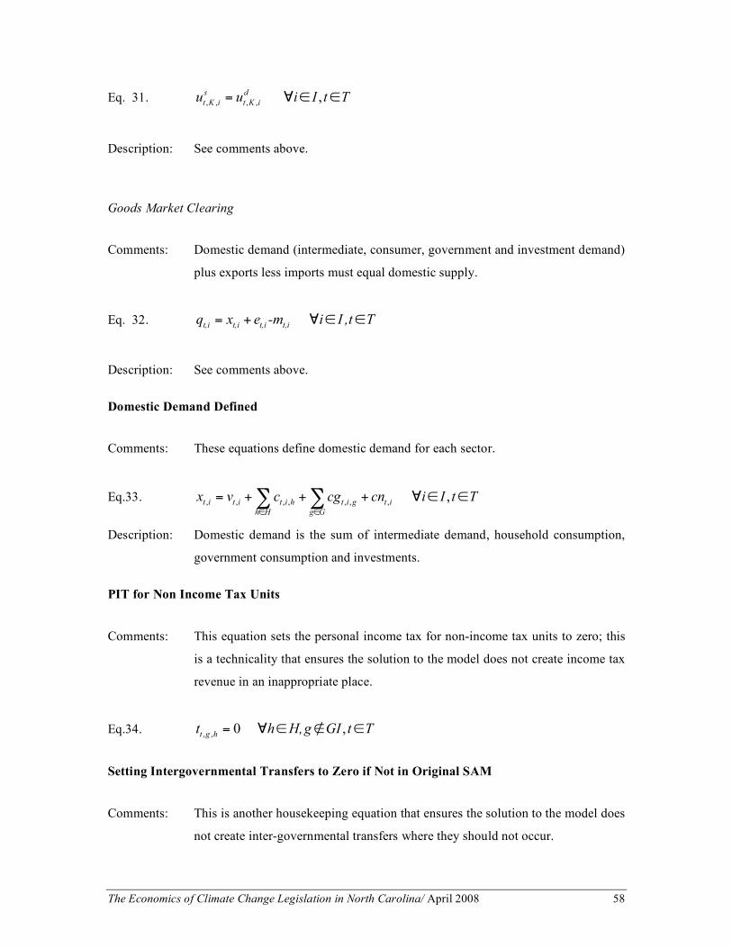
The Economics of Climate Change Legislation in North Carolina/ April 2008 58
Eq. 31. , , , ,
,s d
t K i t K iu u i I t T= ! " "
Description: See comments above.
Goods Market Clearing
Comments: Domestic demand (intermediate, consumer, government and investment demand)
plus exports less imports must equal domestic supply.
Eq. 32. t,i t,i t,i t,i
q x e -m i I ,t T= + ! " "
Description: See comments above.
Domestic Demand Defined
Comments: These equations define domestic demand for each sector.
Eq.33. , , , , , , ,
,t i t i t i h t i g t i
h H g G
x v c cg cn i I t T! !
= + + + " ! !# #
Description: Domestic demand is the sum of intermediate demand, household consumption,
government consumption and investments.
PIT for Non Income Tax Units
Comments: This equation sets the personal income tax for non-income tax units to zero; this
is a technicality that ensures the solution to the model does not create income tax
revenue in an inappropriate place.
Eq.34. , ,
0 ,t g ht h H,g GI t T= ! " # "
Setting Intergovernmental Transfers to Zero if Not in Original SAM
Comments: This is another housekeeping equation that ensures the solution to the model does
not create inter-governmental transfers where they should not occur.
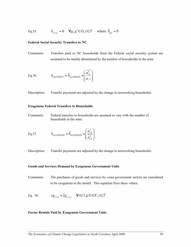
The Economics of Climate Change Legislation in North Carolina/ April 2008 59
Eq.35. , ,
0 , , where 0t g g ggb g g G t T b! !!= " # # =
Federal Social Security Transfers to NC
Comments: Transfers paid to NC households from the Federal social security system are
assumed to be mainly determined by the number of households in the state.
Eq.36. ,
t,h,USSSTX t,h,USSSTX,
n
t h
t h
ab b
a
! "# $= %# $& '
Description: Transfer payments are adjusted by the change in nonworking households.
Exogenous Federal Transfers to Households Comments: Federal transfers to households are assumed to vary with the number of
households in the state.
Eq.37. ,
t,h,USNOND t,h,USNOND
,
n
t h
n
t h
ab b
a
! "# $= %# $& '
Description: Transfer payments are adjusted by the change in nonworking households.
Goods and Services Demand by Exogenous Government Units
Comments: The purchases of goods and services by some government sectors are considered
to be exogenous to the model. This equation fixes these values.
Eq. 38. , , , ,
,t i g t i gcg cg i I,g GX t T= ! " " "
Factor Rentals Paid by Exogenous Government Units

The Economics of Climate Change Legislation in North Carolina/ April 2008 60
Comments: The purchases of the services of labor and capital are considered to be exogenous
to the model. This equation fixes these values.
Eq. 39. , , , ,
,d d
t f g t f gu u f F,g GX t T= ! " " "
Intersectoral Wage Differentials
Comments: Although wage rates differ from sector to sector, these differentials are assumed
to remain fixed, as set by this equation. Household labor supply responds to
overall wage rates, and not to the wage rates in any particular sector.
Eq. 40. , , , ,
,t L i t L i
r r i I t T= ! " "
Government Rental Rate for Capital to Initial Level
Comments: For NC-STAMP, we have set these rental rates to zero, in the absence of viable
information about the rental rates paid by government on the capital that it uses.
However, the relevant equations are included, and so government rental rates
could be incorporated in a future version of the model.
Eq. 41. , , , ,
,t K g t K gr r g G t T= ! " "
Economy Wide Scalar for Capital
Comments: The model allows both for an overall cost of capital, and sector-specific returns.
This equation sets the overall scalar to its original level, so that only the sector-
specific returns vary endogenously.
Eq. 42. , ,
,a a
t K t Kr r f F t T= ! " "
Setting Transfer Payments to Zero

The Economics of Climate Change Legislation in North Carolina/ April 2008 61
Comments: This equation ensures that if transfer payments to households were zero in the
original social accounting matrix, they remain at zero.
Eq. 43. , , , ,
0 , where 0t h g t h gw h H,g GWX t T w= ! " " " =
Objective Function Comments: This equation measures utility over the entire period of the dynamic model as
measured by the sum of state personal income discounted. The variable is of
interest in its own right. However, it is a convenient variable for GAMS to
maximize (or minimize), because it is an unrestricted variable without a
subscript.
Eq. 44. t t
t T
U statey t T!"
= "#
Description: Utility is defined as the net present value of future state personal income levels.
Elasticity Assumptions for NC-STAMP For the model to work, one has to introduce values for the relevant elasticities. These are drawn
from the existing literature, as follows:
ETAM: Import elasticity with respect to domestic price for producers’ purchase of intermediates.
Most of the data on elasticities are taken from Reinert, Roland-Holst, and Shiells. The two most
recent are Reinert and Roland-Holst62 and Roland-Holst, Reinert and Shiells63.
In the first study, the authors estimate an Armington model for 163 mining and manufacturing
sectors. Two-thirds of the elasticities were positive and statistically significant, ranging from a
low of 0.13 for chocolate to 3.49 for wine, brandy and brandy spirits. The second study looked at
the impact of NAFTA. In this study many of the aggregate industries had an elasticity of 1.50.
Since import data for goods between states is almost impossible to obtain, we made some
62Kenneth.A. Reinert and David .W. Roland-Holst, “Armington Elasticities for United States Manufacturing Sectors,” Journal of Policy Modeling 14, no.5 (1992): 631-639. 63 David W. Roland-Holst, Kenneth.A. Reinert and Clinton.R. Shiells, “A General Equilibrium Analysis of North American Economic Integration,” in Modeling Trade Policy: Applied General Equilibrium Assessments of North American Free Trade ed. Clinton .R. Shiells and Joseph F. Francois (New York: Cambridge Univ. Press, 1994), 47-82.

The Economics of Climate Change Legislation in North Carolina/ April 2008 62
assumptions and used 1.50 for most industries and a slightly lower elasticity of 0.50 for a handful
of less traded industries such as service industries.
While these elasticities are slightly higher than the literature on national trade, we believe that
goods in a state are more price-sensitive to goods in the Rest of the World (including other states)
than national goods. Therefore, we converted the elasticities to a domestic share elasticity for
each industry using the following equation. ETAD = ETAM * IMPORT / (DOM. DEMAND *
DOM. SUPPLY SHARE OF DOM. DEMAND). The estimates for this elasticity were taken
from the literature.
ETAE: Export elasticity with respect to domestic price for the sale producers’ goods. Used in the
export demand equation. The NAFTA study was also helpful with exports. We used an elasticity
of 1.65 for industries which had an import elasticity of 1.50 and an export elasticity of 0.65 for
those which had an import elasticity of 0.50.
SIGMA: Elasticity of substitution between capital and labor. Values in the literature range
between 0.15 and 1.809 for industries with the majority close to 1, and we have used values of
0.90 for industries with substantial substitution and 0.8 in other cases (as shown in Table 2). This
measurement is used to calculate RHO, which is the exponent in the production function. The
equation is: RHO = (1- SIGMA)/SIGMA.
The following elasticities are used in household-specific equations:
ETAPIT: Labor supply elasticity with respect to income taxes. This elasticity appears as an
exponent in the labor supply equation. Measurements were based on estimates taken from the
literature. The labor supply elasticities (ETARA) are widely divergent in the literature and suffer
from a lack of disaggregation. They range from close to zero to 2.3 for net wages, with rather
high positive values for women, particularly married woman. This means that the tax elasticities
are negative. There is some evidence of greater (absolute) tax elasticities at higher income levels,
which is why we assume a graduated scale from -0.15 for the lowest income category to -0.35 in
the top category (see Table 10).64
64 Note that ETAPIT = -ETARA (t/(1-t)), where t is the income tax rate.

The Economics of Climate Change Legislation in North Carolina/ April 2008 63
Table 9: Industry Elasticities ETAM ETAE ETAY ETAOP SIGMA AGRICF 1.500000 -1.650000 1.000000 -1.000000 0.900000 MINING 1.500000 -1.650000 1.000000 -1.000000 0.800000 CONSTR 1.500000 -1.650000 1.000000 -1.000000 0.900000 FOODPR 1.500000 -1.650000 1.000000 -1.000000 0.900000 APPARL 1.500000 -1.650000 1.000000 -1.000000 0.900000 MFRCON 1.500000 -1.650000 1.000000 -1.000000 0.800000 PPAPER 1.500000 -1.650000 1.000000 -1.000000 0.800000 CHEMIC 1.500000 -1.650000 1.000000 -1.000000 0.800000 ELECTR 1.500000 -1.650000 1.000000 -1.000000 0.900000 COMPUT 1.500000 -1.650000 1.000000 -1.000000 0.900000 MVOTRA 1.500000 -1.650000 1.000000 -1.000000 0.800000 METALS 1.500000 -1.650000 1.000000 -1.000000 0.800000 MACHIN 1.500000 -1.650000 1.000000 -1.000000 0.900000 MFROTH 1.500000 -1.650000 1.000000 -1.000000 0.900000 TRANSP 1.500000 -1.650000 1.000000 -1.000000 0.900000 INFORM 1.500000 -1.650000 1.000000 -1.000000 0.900000 UTILIT 1.500000 -1.650000 1.000000 -1.000000 0.800000 WHOLSA 0.500000 -0.650000 1.000000 -1.000000 0.900000 RETAIL 0.500000 -0.650000 1.000000 -1.000000 0.900000 BANKNG 1.500000 -1.650000 1.000000 -1.000000 0.900000 INSURS 1.500000 -1.650000 1.000000 -1.000000 0.900000 REALST 1.500000 -1.650000 1.000000 -1.000000 0.900000 PROTEC 1.500000 -1.650000 1.000000 -1.000000 0.800000 MANGAD 1.500000 -1.650000 1.000000 -1.000000 0.800000 HEALTH 0.500000 -0.650000 1.000000 -1.000000 0.800000 ENTRHO 0.500000 -0.650000 1.000000 -1.000000 0.800000 OTHSVC 0.500000 -0.650000 1.000000 -1.000000 0.800000 USNOND 0 0 0 0 0 USDEFF 0 0 0 0 0 STGGSP 0 0 0 0 0 STEDUC 0 0 0 0 0 STHELT 0 0 0 0 0 STPBSF 0 0 0 0 0 STTRAN 0 0 0 0 0 STOTHS 0 0 0 0 0 LOEDUC 0 0 0 0 0 LOHELT 0 0 0 0 0 LOPBSF 0 0 0 0 0 LOTRAN 0 0 0 0 0 LOOTHS 0 0 0 0 0

The Economics of Climate Change Legislation in North Carolina/ April 2008 64
ETATP: Household response to transfer payments. The transfer payment elasticities reflect a
study by Robins on the effects of a negative income tax (NIT).65 It is also a reflection of the
observation that income received by upper income groups is on average largely unaffected by
transfer payments.
ETAYD: Responsiveness of immigration to after tax income. The tying of migration to
disposable income or unemployment finds little support in the economic literature. Studies by
Bartik and others put the range of responses to a change in wage rates at between 0.835 and
2.39.66 We used these as a basis for our after tax earnings elasticities. This elasticity appears in
the population equation.
ETAU: Responsiveness of immigration to unemployment. We made some assumptions based on
the responsiveness to employment elasticities in the literature.
ETAMH: Income elasticity of demand for imports by household. This elasticity appears in the
household import equation.
Table 10 provides elasticities, a summary of set names and a summary of parameter names.
Table 10: Household Related Elasticities
ETAPIT ETATP ETARA ETAYD ETAU ETAMH
LESS10 -0.15 -0.05 0.17 1.30 -0.80 0.70 LESS25 -0.18 -0.05 0.17 1.50 -0.80 0.70 LESS50 -0.20 -0.04 0.20 1.60 -0.80 0.70 LESS75 -0.25 -0.04 0.30 1.80 -0.80 0.70 LES100 -0.25 -0.03 0.40 2.00 -0.80 0.70 LES150 -0.30 -0.03 0.50 2.10 -0.80 0.70 MOR150 -0.35 -0.02 0.50 2.30 -0.80 0.70
65 Phillip K. Robins, “A Comparison of the Labor Supply Findings from the Four Negative Income Tax Experiments.” Journal of Human Resources 20 (1985): 567-82. 66 For one response see Timothy Bartik, Who Benefits from State and Local Economic Development Policy? (Kalamazoo: W.E. Upjohn Institute for Employment Research, 1991).

The Economics of Climate Change Legislation in North Carolina/ April 2008 65
Table 11: Summary of Set Names Sets Dimension Math GAMS Factors 2 f∈F F Governments – All 39 g∈G G Governments - Factor Taxes 6 g∈GF GF Governments - Per Household Taxes 8 g∈GH GH Governments - Income Taxes 2 g∈GI GI Governments - Capital Income Taxes 6 g∈GK GK Governments - Endogenous Spending 16 g∈GN GN Governments - Sales or Excise Taxes 11 g∈GS GS Governments - Endogenous Transfer Payments 1 g∈GWN GWN Governments - Exogenous Transfer Payments 4 g∈GWX GWX Governments - Exogenous Spending 6 g∈GX GX Households 7 h∈H H Industries 27 i∈I or j∈I I All Social Accounting Matrix Accounts 77 z∈Z Z
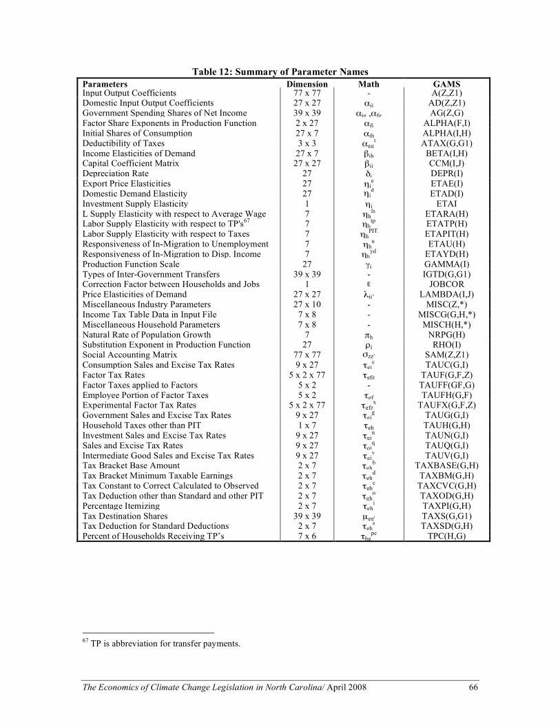
The Economics of Climate Change Legislation in North Carolina/ April 2008 66
Table 12: Summary of Parameter Names Parameters Dimension Math GAMS Input Output Coefficients 77 x 77 - A(Z,Z1) Domestic Input Output Coefficients 27 x 27
αij AD(Z,Z1)
Government Spending Shares of Net Income 39 x 39 αig ,αfg AG(Z,G) Factor Share Exponents in Production Function 2 x 27
αfi ALPHA(F,I)
Initial Shares of Consumption 27 x 7 αih ALPHA(I,H) Deductibility of Taxes 3 x 3 αgg
t ATAX(G,G1) Income Elasticities of Demand 27 x 7 βih BETA(I,H) Capital Coefficient Matrix 27 x 27 βij CCM(I,J) Depreciation Rate 27 δi DEPR(I) Export Price Elasticities 27 ηi
e ETAE(I) Domestic Demand Elasticity 27 ηi
d ETAD(I) Investment Supply Elasticity 1 ηi ETAI L Supply Elasticity with respect to Average Wage 7 ηh
ls ETARA(H) Labor Supply Elasticity with respect to TP's67
7 ηhtp ETATP(H)
Labor Supply Elasticity with respect to Taxes
7 ηhPIT ETAPIT(H)
Responsiveness of In-Migration to Unemployment 7 ηhu ETAU(H)
Responsiveness of In-Migration to Disp. Income 7 ηhyd ETAYD(H)
Production Function Scale 27 γi GAMMA(I) Types of Inter-Government Transfers 39 x 39 - IGTD(G,G1) Correction Factor between Households and Jobs 1 ε JOBCOR Price Elasticities of Demand 27 x 27 λii’ LAMBDA(I,J) Miscellaneous Industry Parameters 27 x 10 - MISC(Z,*) Income Tax Table Data in Input File 7 x 8 - MISCG(G,H,*) Miscellaneous Household Parameters 7 x 8 - MISCH(H,*) Natural Rate of Population Growth 7 πh NRPG(H) Substitution Exponent in Production Function 27
ρi RHO(I)
Social Accounting Matrix 77 x 77 σzz’ SAM(Z,Z1) Consumption Sales and Excise Tax Rates 9 x 27 τgi
c TAUC(G,I) Factor Tax Rates 5 x 2 x 77 τgfz TAUF(G,F,Z)
Factor Taxes applied to Factors 5 x 2 - TAUFF(GF,G) Employee Portion of Factor Taxes 5 x 2 τgf TAUFH(G,F) Experimental Factor Tax Rates 5 x 2 x 77 τgfz
x TAUFX(G,F,Z) Government Sales and Excise Tax Rates 9 x 27 τgi
g TAUG(G,I) Household Taxes other than PIT 1 x 7 τgh TAUH(G,H)
Investment Sales and Excise Tax Rates 9 x 27 τgin TAUN(G,I)
Sales and Excise Tax Rates 9 x 27 τqiq TAUQ(G,I)
Intermediate Good Sales and Excise Tax Rates 9 x 27 τgiv TAUV(G,I)
Tax Bracket Base Amount 2 x 7 τghb TAXBASE(G,H)
Tax Bracket Minimum Taxable Earnings 2 x 7 τghd TAXBM(G,H)
Tax Constant to Correct Calculated to Observed 2 x 7 τghc TAXCVC(G,H)
Tax Deduction other than Standard and other PIT 2 x 7 τgho TAXOD(G,H)
Percentage Itemizing 2 x 7 τghi TAXPI(G,H)
Tax Destination Shares 39 x 39 µgg' TAXS(G,G1) Tax Deduction for Standard Deductions 2 x 7 τgh
s TAXSD(G,H) Percent of Households Receiving TP’s 7 x 6 τhg
pc TPC(H,G)
67 TP is abbreviation for transfer payments.

The Economics of Climate Change Legislation in North Carolina/ April 2008 67
Table 12 (Continued) Variables Dimension Math GAMS Public Consumption 27 x 39 cig CG(I,G) Private Consumption 27 x 7 cih CH(I,H) Gross Investment by Sector of Source 27 cin CN(I) Consumer Price Index 7 ph CPI(H) Exports 27 ei CX(I) Domestic Share of Domestic Consumption 27 di D(I) Domestic Demand 27 xi DD(I) Domestic Supply 27 qi DS(I) Sectoral Factor Demand 2 x 77 ufi
d, ufgd FD(F,Z)
Number of Households 7 ah HH(H) Number of Non-Working Households 7 ah
n HN(H) Number of Working Households 7 ah
w HW(H) Household Out-Migration 7 ah
o MO(H) Household In-Migration 7 ah
i MI(H) Inter-Governmental Transfers 37 x 37 Bgg’ IGT(G,G1) Capital Stock 27 uKi
s KS(I) Imports 27 mi M(I) Gross Investment by Sector of Destination 27 ni N(I) Net Capital Inflow 1 z NKI Aggregate Price 27 pi P(I) Aggregate Price including Sales/Excise Taxes 27 pi
c PC(I) Domestic Producer Price 27 pi
d PD(I) Per Household Personal Income Taxes 2 x 7 tgh PIT(G,H) Producer Price Index 1 p PPI Value Added Price 27 pi
va PVA(I) World Price (Rest of US and Rest of World) 27 pi
w PW(I) Sectoral Factor Rental Rates 2 x 27 rfi, rfg R(F,I) Economy Wide Scalar for Factor Rental Rates 2 rf
a RA(F) Government Savings 39 sg S(G) Private Savings 7 sh S(H) State Personal Income 1 q SPI Transfer Payments 7 x 39 whg TP(H,G) Intermediate Goods 27 vi V(I) Factor Income 2 yf Y(F) Government Income 39 yg Y(G) Household Income 7 yh Y(H) Household after Tax Income including TP’s 7 Yh
d YD(H)

The Economics of Climate Change Legislation in North Carolina/ April 2008 68
Bibliography American Council for Capital Formation and National Association of Manufacturers. Analysis of
Lieberman-Warner Climate Security Act (S. 2191) Using the National Energy Modeling System. (March 13, 2008). http://www.accf.org/pdf/NAM/fullstudy031208.pdf.(accessed April 17, 2008).
America's Climate Security Act of 2007, S 2191, 110th Cong. 1st session, GovTrack.us.
http://www.govtrack.us/congress/bill.xpd?bill=s110-2191. (accessed April 17, 2008). Armington, Paul. "A Theory of Demand for Products Distinguished by Place of Production."
International Monetary Fund Staff Papers 16 (1969): 159-78. Berck, Peter, Elise Golan, and B. Smith, with John Barnhart, and Andrew Dabalen. “Dynamic
Revenue Analysis for California.” University of California at Berkeley and California Department of Finance (1996): 117. http://www.dof.ca.gov. (accessed April 17, 2008). Center for Climate Strategies. Memorandum to North Carolina Climate Action Plan Advisory
Group. February 16, 2006, http://www.ncclimatechange.us/capag.cfm. General Assembly of North Carolina. An Act to Establish the Legislative Commission on Global
Warming, S 1134, Session Law 2005-442 (September 27, 2005). http://www.ncleg.net/gascripts/DocumentSites/browseDocSite.asp?nID=14&sFolderName=\Authorizing%20Legislation.
Harris, John R. and Michael P. Todaro. “Migration, Unemployment and Development: A Two
Sector Analysis.” American Economic Review 40 (1970): 126-42. LaCarpa Associates. Analysis of a Renewable Portfolio Standard for the State of North Carolina
(December, 2006): 61. http://www.ncuc.net/rps/rps.htm. (accessed April 17, 2008). North Carolina Climate Action Plan Advisory Group. “Recommended Mitigation Options for
Controlling Greenhouse Gas Emissions: Draft Final Report.” (October 2007). http://www.ncclimatechange.us/capag.cfm; 1-11. (accessed April 17, 2008).
North Carolina State Energy Office. North Carolina State Energy Plan. (June 2003, Revised
Edition, January 2005): 74 Ponder, David and Jeffry Tiller. “Preliminary Draft Results, Economic Impact Analysis of
Bundled Climate Mitigation Options: Prepared for the North Carolina Climate Action Advisory Group.” October 27, 2007. PowerPoint Presentation.
Reinert, Kenneth A.and David W. Roland-Holst. “Armington Elasticities for United States
Manufacturing Sectors.” Journal of Policy Modeling 14, no.5 (1992): 631-639.

The Economics of Climate Change Legislation in North Carolina/ April 2008 69
Robins, Phillip K. “A Comparison of the Labor Supply Findings from the Four Negative Income Tax Experiments.” Journal of Human Resources 20 (1985): 567-82. Roland-Holst, David W., Kenneth A. Reinert, and Clinton.R. Shiells. “A General Equilibrium
Analysis of North American Economic Integration.” Modeling Trade Policy: Applied General Equilibrium Assessments of North American Free Trade ed. Clinton R. Shiells and Joseph F. Francois. (New York: Cambridge Univ. Press, 1994): 47-82.
Rose, Adam and Dan Wei. “Review of North Carolina Energy Scenario Economic Impact
Model.” Pennsylvania State University (November 29, 2005): 5. Shoven, John B. and John Whalley. “Applied General-Equilibrium Models of Taxation and International Trade: An Introduction and Survey.” Journal of Economic Literature 22 (September, 1984): 1008. Tuerck, David G., Jonathan Haughton, In-Mee Baek, James Connolly, and Scott Fontaine. The
Texas State Tax Analysis Modeling Program: Methodology and Applications. The Beacon Hill Institute at Suffolk University. (February 1999).
U. S. Congress. America's Climate Security Act of 2007, S 2191, 110th Cong. 1st session,
GovTrack.us. http://www.govtrack.us/congress/bill.xpd?bill=s110-2191. (accessed April 17, 2008).
U.S. Department of Commerce, Bureau of Economic Analysis. “Underlying Detail for the
National Income and Product Account Tables.” http://www.bea.doc.gov/, table 7.2.5S. (accessed April 17, 2008).
U.S. Department of Energy, Energy Information Administration. Annual Energy Outlook: 2008
(Early Release). “Table 3. Energy Prices by Sector and Source.” http://www.eia.doe.gov/oiaf/aeo/excel/aeotab_3.xls (accessed April 17, 2008).
_______________________. Energy Information Administration. “Energy Consumption by
Sector and Source” in “Table 2: Energy Price and Expenditure Estimates by Source, 1970-2005, North Carolina.” http://www.eia.doe.gov/oiaf/aeo/excel/aeotab_2.xls. (accessed April 17, 2008).
_______________________. Energy Information Administration. “Forecasts and Analysis,
Alternative Fuels: Ethanol.” http://www.eia.doe.gov/oiaf/ethanol3.html. (accessed April 17, 2008).
________________________. Energy Information Administration. “Table C4: Estimated
Consumption of Alternative Fuels by State and Fuel Type, 2005.” http://www.eia.doe.gov/cneaf/alternate/page/atftables/afvtransfuel_II.html (accessed April 17, 2008).
________________________. Energy Information Administration. “Table 1:
Energy Price and Expenditure Estimates by Source, 1970-2005, North Carolina.” http://www.eia.doe.gov/states/sep_prices/total/pr_tot_nc.html. (accessed April 17, 2008).

The Economics of Climate Change Legislation in North Carolina/ April 2008 70
U.S. Department of Transportation. Bureau of Transportation Statistics. “State Transportation Statistics 2006 in “Table 7-4: Motor Fuel Use: 2005.” http://www.bts.gov/publications/state_transportation_statistics/state_transportation_statistics_2006/html/table_07_04.html. (accessed April 17, 2008).
_________________________. Bureau of Transportation Statistics. “State Transportation
Statistics 2005,” in “Table 5-1: Motor-Vehicle Registrations.” http://www.bts.gov/publications/state_transportation_statistics/state_transportation_statistics_2005/index.html. (accessed April 17, 2008).

The Economics of Climate Change Legislation in North Carolina/ April 2008 71
The Beacon Hill Institute North Carolina-STAMP Development Team
David G. Tuerck is Executive Director of the Beacon Hill Institute for Public Policy Research at Suffolk University where he also serves as Chairman and Professor of Economics. He holds a Ph.D. in economics from the University of Virginia and has written extensively on issues of taxation and public economics. Alfonso Sanchez-Penalver is an Economist at the Beacon Hill Institute. He holds a Master of Science degree in Finance from Boston College, and a BSBA in Finance from Suffolk University. He is currently enrolled in the PhD program in Economics at Suffolk University. He has an extensive career in web programming and project management, as well as in accounting and financial analysis. Vadym Slobodyanyuk is a consulting Economist with the Beacon Hill Institute. He holds a Master of Science in International Economics degree from Suffolk University and a Bachelor of Arts (economics) degree from the University of Kyiv-Mohyla Academy, Ukraine. He has five years experience working closely with the STAMP model. Paul Bachman is Director of Research at BHI. He manages the institute's research projects, including the STAMP model and conducts research on other projects at the BHI. Mr. Bachman has authored research papers on state and national tax policy and on state labor policy and produces the institute’s state revenue forecasts for the Massachusetts legislature. He holds a Master Science in International Economics from Suffolk University. Michael Head is a Research Economist at BHI. He holds a Master of Science in Economic Policy from Suffolk University. The authors would like to thank Frank Conte, BHI Director of Communications, for editorial assistance.

The Economics of Climate Change Legislation in North Carolina/ April 2008 72
The Beacon Hill Institute at Suffolk University in Boston focuses on federal, state and local economic policies as they affect citizens and businesses. The institute conducts research and educational programs to provide timely, concise and readable analyses that help voters, policymakers and opinion leaders understand today’s leading public policy issues.
©April 2008 by the Beacon Hill Institute at Suffolk University
THE BEACON HILL INSTITUTE FOR PUBLIC POLICY RESEARCH
Suffolk University 8 Ashburton Place Boston, MA 02108
Phone: 617-573-8750 Fax: 617-994-4279 [email protected]
http://www.beaconhill.org


![Legislation Review Committee · Parliament. Legislative Assembly. Legislation Review Committee Legislation Review Digest, Legislation Review Committee, Parliament NSW [Sydney, NSW]:](https://static.fdocuments.in/doc/165x107/5f9c6bc6de302b4245453c3b/legislation-review-committee-parliament-legislative-assembly-legislation-review.jpg)