The economic impact of climate change
33
The Economic Impacts of Climate Change: Evidence from Agricultural Output and Random Fluctuations in Weather By OLIVIER DESCHE ˆ NES AND MICHAEL GREENSTONE* This paper measures the economic impact of climate change on US agricultural land by estimating the effect of random year-to-year variation in temperature and precipitation on agricultural profits. The preferred estimates indicate that climate change will increase annual profits by $1.3 billion in 2002 dollars (2002$) or 4 percent. This estimate is robust to numerous specification checks and relatively precise, so large negative or positive effects are unlikely. We also find the hedonic approach—which is the standard in the previous literature—to be unreliable be- cause it produces estimates that are extremely sensitive to seemingly minor choices about control variables, sample, and weighting. ( JEL L25, Q12, Q51, Q54) There is a growing consensus that emissions of greenhouse gases due to human activity will lead to higher temperatures and increased pre- cip itatio n. It is tho ugh t tha t these cha nge s in climate will have an impact on economic well- being. Since temperature and precipitation are direc t input s in agric ultur al produ ction, many believe that the largest effects will be in this sec tor . Pre vious res ear ch on cli mat e cha nge concerning the sign and magnitude of its effect on the value of US agricultural land is incon- clusive (see, for example, Richard M. Adams 1989; Robert Mendelsoh n, Wil lia m D. Nord- haus, and Daigee Shaw 1999; David L. Kelly, Char les D. Kols tad, and Glenn T. Mitchell 2005; Wolfram Schlenker, W. Michael Hane- mann, and Anthony C. Fisher (henceforth, SHF) 2005, 2006) . Most prior research employs either the pro- duction function or hedonic approach to esti- mate the effect of climate change. 1 Due to its exp eri mental des ign , the pro duction fun ction app roa ch pro vides est ima tes of the eff ect of weather on the yields of specific crops that are purged of bias due to determinants of agricul- tur al out put tha t are bey ond farmers’ con trol (e.g., soil quality). Its disadvantage is that these * Desche ˆnes : Department of Ec onomics, Univer sity of Cal- ifornia, Santa Barbara, 2127 North Hall, Santa Barbara, CA 93106 (e-mail: [email protected]); Greenstone: MIT De- partment of Economics, E52-359, 50 Memorial Drive, Cam- brid ge, MA 0214 2-13 47 (e-mail: mgre enst @mit .edu ). We thank the late David Bradford for initiating a conversation that motivated this paper. Our admiration for David’s brilliance as an economist was exceeded only by our admiration for him as a human being. We are grateful for the especially valuable criticisms from David Card and two anonymous referees. Orley Ashenfelter, Doug Bernheim, Hoyt Bleakley, Tim Con- ley, Tony Fisher, Victor Fuchs, Larry Goulder, Michael Hane- mann, Barrett Kirwan, Charlie Kolstad, Enrico Moretti, Marc Nerlove, Jess e Roth stei n, and Wolf ram Schl enke r prov ided insightful comments. We are also grateful for comments from semi nar part icip ants at Corn ell Universi ty, Universi ty of Mary - land, Princeton University, University of Illinois at Urbana- Cham paig n, Stan ford Univ ersi ty, and Yale Univ ersi ty, the NBER Environmental Economics Summer Institute, and the “Conference on Spatial and Social Interactions in Economics” at the University of California-Santa Barbara. Anand Dash, Eliz abet h Gree nwoo d, Ben Hans en, Barr ett Kirwan, Nick Nagle, and William Young provided outstanding research as- sistance. We are indebted to Shawn Bucholtz at the United States Depa rtme nt of Agri cult ure for gene rous ly gene rati ng weather data for this analysis from the Para mete r-elevat ion Regr essi ons on Inde pend ent Slop es Mode l. Fina lly, we ac- knowledge the Vegetation/Ecosystem Modeling and Analysis Project and the Atmosphere Section, National Center for At- mospheric Research, for access to the Transient Climate data- base, whi ch we us ed to obt ain re gio na l cli ma te ch ang e predictions. Greenstone acknowledges generous funding from the Ameri can Bar Fou nda tio n, the Cen ter for Ene rgy and Environmental Policy Research at MIT, and the Center for Labor Economics at UC-Berkeley for hospitality and support whil e work ing on this pape r. Desc he ˆnes than ks the UCSB Academic Senate for financial support and the Industrial Re- lations Section at Princeton University for their hospitality and support while working on this paper. 1 Throughout, “weather” refers to temperature and pre- cipitation at a given time and place. “Climate” or “climate normals” refer to a location’s weather averaged over long periods of time. 354
description
This paper measures the economic impact of climate change on US agriculturalland by estimating the effect of random year-to-year variation in temperature andprecipitation on agricultural profits
Transcript of The economic impact of climate change
7/18/2019 The economic impact of climate change
http://slidepdf.com/reader/full/the-economic-impact-of-climate-change 1/32
The Economic Impacts of Climate Change: Evidence from
Agricultural Output and Random Fluctuations in Weather
By OLIVIER DESCHENES AND MICHAEL GREENSTONE*
This paper measures the economic impact of climate change on US agriculturalland by estimating the effect of random year-to-year variation in temperature and
precipitation on agricultural profits. The preferred estimates indicate that climatechange will increase annual profits by $1.3 billion in 2002 dollars (2002$) or 4
percent. This estimate is robust to numerous specification checks and relatively precise, so large negative or positive effects are unlikely. We also find the hedonicapproach—which is the standard in the previous literature—to be unreliable be-cause it produces estimates that are extremely sensitive to seemingly minor choicesabout control variables, sample, and weighting. ( JEL L25, Q12, Q51, Q54)
There is a growing consensus that emissionsof greenhouse gases due to human activity willlead to higher temperatures and increased pre-cipitation. It is thought that these changes in
climate will have an impact on economic well-being. Since temperature and precipitation aredirect inputs in agricultural production, manybelieve that the largest effects will be in thissector. Previous research on climate changeconcerning the sign and magnitude of its effecton the value of US agricultural land is incon-clusive (see, for example, Richard M. Adams1989; Robert Mendelsohn, William D. Nord-
haus, and Daigee Shaw 1999; David L. Kelly,Charles D. Kolstad, and Glenn T. Mitchell2005; Wolfram Schlenker, W. Michael Hane-mann, and Anthony C. Fisher (henceforth, SHF)2005, 2006).
Most prior research employs either the pro-duction function or hedonic approach to esti-mate the effect of climate change.1 Due to itsexperimental design, the production functionapproach provides estimates of the effect of weather on the yields of specific crops that arepurged of bias due to determinants of agricul-tural output that are beyond farmers’ control(e.g., soil quality). Its disadvantage is that these
* Deschenes: Department of Economics, University of Cal-ifornia, Santa Barbara, 2127 North Hall, Santa Barbara, CA93106 (e-mail: [email protected]); Greenstone: MIT De-partment of Economics, E52-359, 50 Memorial Drive, Cam-bridge, MA 02142-1347 (e-mail: [email protected]). Wethank the late David Bradford for initiating a conversation thatmotivated this paper. Our admiration for David’s brilliance asan economist was exceeded only by our admiration for him asa human being. We are grateful for the especially valuablecriticisms from David Card and two anonymous referees.Orley Ashenfelter, Doug Bernheim, Hoyt Bleakley, Tim Con-ley, Tony Fisher, Victor Fuchs, Larry Goulder, Michael Hane-mann, Barrett Kirwan, Charlie Kolstad, Enrico Moretti, MarcNerlove, Jesse Rothstein, and Wolfram Schlenker providedinsightful comments. We are also grateful for comments fromseminar participants at Cornell University, University of Mary-land, Princeton University, University of Illinois at Urbana-Champaign, Stanford University, and Yale University, theNBER Environmental Economics Summer Institute, and the“Conference on Spatial and Social Interactions in Economics”at the University of California-Santa Barbara. Anand Dash,Elizabeth Greenwood, Ben Hansen, Barrett Kirwan, Nick Nagle, and William Young provided outstanding research as-sistance. We are indebted to Shawn Bucholtz at the UnitedStates Department of Agriculture for generously generatingweather data for this analysis from the Parameter-elevationRegressions on Independent Slopes Model. Finally, we ac-knowledge the Vegetation/Ecosystem Modeling and AnalysisProject and the Atmosphere Section, National Center for At-mospheric Research, for access to the Transient Climate data-base, which we used to obtain regional climate changepredictions. Greenstone acknowledges generous funding fromthe American Bar Foundation, the Center for Energy and
Environmental Policy Research at MIT, and the Center forLabor Economics at UC-Berkeley for hospitality and supportwhile working on this paper. Deschenes thanks the UCSBAcademic Senate for financial support and the Industrial Re-lations Section at Princeton University for their hospitality andsupport while working on this paper.
1 Throughout, “weather” refers to temperature and pre-cipitation at a given time and place. “Climate” or “climatenormals” refer to a location’s weather averaged over longperiods of time.
354

7/18/2019 The economic impact of climate change
http://slidepdf.com/reader/full/the-economic-impact-of-climate-change 2/32
estimates do not account for the full range of compensatory responses to changes in weathermade by profit-maximizing farmers. For exam-ple, in response to a change in climate, farmersmay alter their use of fertilizers, change their
mix of crops, or even decide to use their farm-land for another activity (e.g., a housing com-plex). Since farmer adaptations are completelyconstrained in the production function ap-proach, it is likely to produce estimates of cli-mate change that are biased downward.
The hedonic approach attempts to measuredirectly the effect of climate on land values. Itsclear advantage is that if land markets are op-erating properly, prices will reflect the presentdiscounted value of land rents into the infinite
future. In principle, this approach accounts forthe full range of farmer adaptations. Its validity,however, rests on the consistent estimation of the effect of climate on land values. Since atleast the classic Irving Hoch (1958, 1962) andYair Mundlak (1961) papers, it has been recog-nized that unmeasured characteristics (e.g., soilquality and the option value to convert to a newuse) are important determinants of output andland values in agricultural settings.2 Conse-quently, the hedonic approach may confoundclimate with other factors, and the sign and
magnitude of the resulting omitted variablesbias is unknown.
In light of the importance of the question, thispaper proposes a new strategy to estimate theimpact of climate change on the agriculturalsector. The most well respected climate changemodels predict that temperatures and precipita-tion will increase in the future. This paper’s ideais simple—we exploit the presumably randomyear-to-year variation in temperature and pre-cipitation to estimate whether agricultural prof-
its are higher or lower in years that are warmerand wetter. Specifically, we estimate the im-pacts of temperature and precipitation on agri-cultural profits and then multiply them by thepredicted change in climate to infer the eco-nomic impact of climate change in this sector.
To conduct the analysis, we compiled themost detailed and comprehensive data available
to form a county-level panel on agriculturalprofits and production, soil quality, climate, andweather. These data are used to estimate theeffect of weather on agricultural profits andyields, conditional on county and state by year
fixed effects. Thus, the weather parameters areidentified from the county-specific deviations inweather from the county averages after adjust-ing for shocks common to all counties in a state.Put another way, the estimates are identifiedfrom comparisons of counties within the samestate that had positive weather shocks with onesthat had negative weather shocks, after account-ing for their average weather realization.
This variation is presumed to be orthogonalto unobserved determinants of agricultural prof-
its, so it offers a possible solution to the omittedvariables bias problems that plague the hedonicapproach. The primary limitation to this ap-proach is that farmers cannot implement the fullrange of adaptations in response to a singleyear’s weather realization. Consequently, its es-timates may overstate the damage associatedwith climate change or, put another way, bedownward-biased.
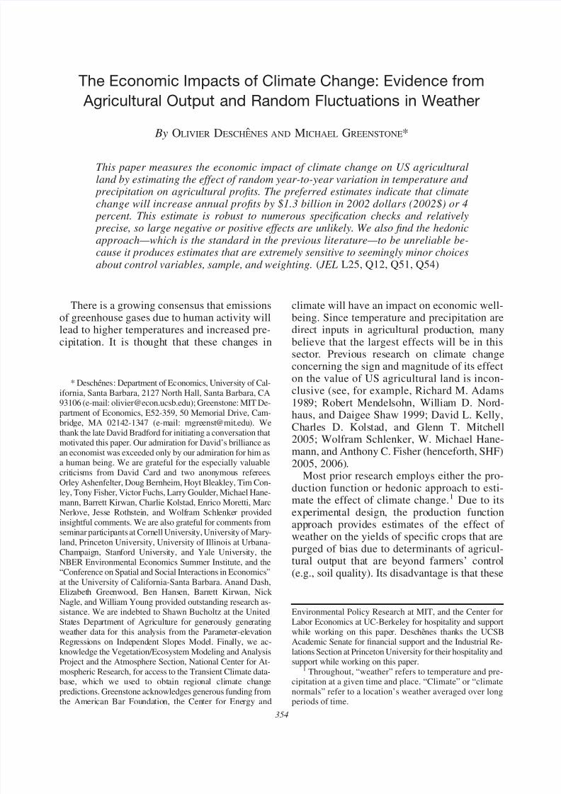
Figures 1A and 1B summarize the paper’sprimary findings. These figures show the fittedquadratic relationships between aggregate agri-
cultural profits, the value of the corn harvest,and the value of the soybean harvest with grow-ing season degree-days (1A) and total precipi-tation (1B). (These measures of temperature andprecipitation are the standard in the agronomyliterature.) The key features of these estimatesare that they are conditioned on county fixedeffects, so the relationships are identified fromthe presumably random variation in weatherwithin a county across years. The estimatingequations also include state by year fixed ef-
fects. The vertical lines correspond to the na-tional averages of growing season degree-daysand precipitation. The average county is pre-dicted to have increases of roughly 1,200degree-days and 3 inches of precipitation duringthe growing season.
The striking finding is that all of the responsesurfaces are flat over the ranges of the predictedchanges in degree-days and inches. If anything,climate change appears to be slightly beneficialfor profits and yields. This qualitative findingholds throughout the battery of tests presentedbelow.
2 Mundlak focused on heterogeneity in the skills of farm-ers, but in Mundlak (2001), he writes, “Other sources of farm-specific effects are differences in land quality, micro-climate, and so on” (9).
355VOL. 97 NO. 1 DESCHE ˆ NES AND GREENSTONE: COST OF CLIMATE CHANGE FOR US AGRICULTURE
7/18/2019 The economic impact of climate change
http://slidepdf.com/reader/full/the-economic-impact-of-climate-change 3/32
Using long-run climate change predictions,the preferred estimates indicate that climatechange will lead to a $1.3 billion (2002$) or4.0-percent increase in annual agriculturalsector profits. The 95-percent confidence in-terval ranges from $0.5 billion to $3.1 bil-lion, so large negative or positive effects are
unlikely. The basic finding of an economi-cally and statistically small effect is robust toa wide variety of specification checks, includ-ing adjustment for the rich set of availablecontrols, modeling temperature and precipita-tion flexibly, estimating separate regressionequations for each state, and implementing a
0
5
10
15
20
25
30
35
40
0 1,000 2,000 3,000 4,000 5,000
Growing season degree-days
B i l l i o n
d o l l a r s
( 2 0 0 2 $ )
Value of corn produced Value of soybeans produced Total profits
FIGURE 1A. FITTED RELATIONSHIP BETWEEN AGGREGATE PROFITS (TOTAL VALUE OF CROPSPRODUCED) AND GROWING SEASON DEGREE-DAYS
0
5
10
15
20
25
30
35
40
0 10 20 30 40 50 60
Growing season precipitation
B
i l l i o n
d o l l a r s ( $ 2 0 0 2 )
Value of corn produced Value of soybeans produced Total profits
FIGURE 1B. FITTED RELATIONSHIP BETWEEN AGGREGATE PROFITS (TOTAL VALUE OF CROPS
PRODUCED) AND GROWING SEASON PRECIPITATION
Notes: Underlying the figure are quadratic regressions of profits per acre and yields per acreplanted on growing season degree-days (A) and total precipitation (B). The crop yield per acrevalues are converted to an aggregate figure by multiplying the regression estimates by the
1987–2002 average crop price per bushel and by the 1987–2002 average aggregate acreageplanted in the relevant crop. The profit per acre values are converted to an aggregate figure bymultiplying the regression estimates by the 1987–2002 average aggregate acreage in farms. Theregressions also include county fixed effects and state by year fixed effects and are weighted byacres of farmland (profits models) or acres planted in the relevant crop (crop yield models).
356 THE AMERICAN ECONOMIC REVIEW MARCH 2007

7/18/2019 The economic impact of climate change
http://slidepdf.com/reader/full/the-economic-impact-of-climate-change 4/32
procedure that minimizes the influence of out-liers. Additionally, the analysis indicates thatthe predicted increases in temperature and pre-cipitation will have virtually no effect on yieldsof the most important crops (i.e., corn for grain
and soybeans). These crop yield findings sug-gest that the small effect on profits is not due toshort-run price increases.
Although the overall effect is small, there isconsiderable heterogeneity across the country.The most striking finding is that California willbe harmed substantially by climate change. Itspredicted loss in agricultural profits is $750million, nearly 15 percent of current annualprofits in California. Nebraska ($670 million)and North Carolina ($650 million) are also
predicted to have big losses, while the two biggestwinners are South Dakota ($720 million) andGeorgia ($540 million). It is important to note thatthese state-level estimates are based on fewer ob-servations than the national estimates and there-fore their precision is less than ideal.
The paper also reexamines the hedonic ap-proach that is predominant in the previous lit-erature. We find that estimates of the effect of the benchmark doubling of greenhouse gases onthe value of agricultural land range from $200billion (2002$) to $320 billion (or 18 percent
to 29 percent), which is an even wider rangethan has been noted in the previous literature.This variation in predicted impacts results fromseemingly minor decisions about the appropri-ate control variables, sample, and weighting.Despite its theoretical appeal, we conclude thatthe hedonic method may be unreliable in thissetting.3
The paper proceeds as follows. Section I pro-vides the conceptual framework for our ap-proach. Section II describes the data sources
and provides summary statistics. Section IIIpresents the econometric approach and SectionIV describes the results. Section V assesses themagnitude of our estimates of the effect of climate change and discusses a number of im-portant caveats to the analysis. Section VI con-cludes the paper.
I. Conceptual Framework
A. A New Approach to Valuing ClimateChange
In this paper, we propose a new strategy toestimate the effects of climate change. We use acounty-level panel data file constructed fromthe Census of Agriculture to estimate the effectof weather on agricultural profits, conditionalon county and state by year fixed effects. Thus,the weather parameters are identified from thecounty-specific deviations in weather about thecounty averages after adjustment for shockscommon to all counties in a state. This variationis presumed to be orthogonal to unobserved
determinants of agricultural profits, so it offers apossible solution to the omitted variables biasproblems that appear to plague the hedonicapproach.
This approach differs from the hedonic one ina few key ways. First, under an additive sepa-rability assumption, its estimated parameters arepurged of the influence of all unobserved timeinvariant factors. Second, it is not feasible to useland values as the dependent variable once thecounty fixed effects are included. This is be-cause land values reflect long-run averages of
weather, not annual deviations from these aver-ages, and there is no time variation in suchvariables.
Third, although the dependent variable is notland values, our approach can be used to ap-proximate the effect of climate change on agri-cultural land values. Specifically, we estimatehow farm profits are affected by increases intemperature and precipitation. We then multiplythese estimates by the predicted changes in cli-mate to infer the impact on profits. If we assume
the predicted change in profits is permanent andmake an assumption about the discount rate, itis straightforward to calculate the change inland values. This is because the value of land isequal to the present discounted stream of rentalrates.
B. The Economics of Using Annual Variationin Weather to Infer the Impacts of Climate
Change
There are two economic issues that couldundermine the validity of using the relationship
3 Recent research demonstrates that cross-sectional he-donic equations appear misspecified in a variety of contexts(Sandra E. Black 1999; Dan A. Black and Thomas J.Kneisner 2003; Kenneth Y. Chay and Michael Greenstone2005; Greenstone and Justin Gallagher 2005).
357 VOL. 97 NO. 1 DESCHE ˆ NES AND GREENSTONE: COST OF CLIMATE CHANGE FOR US AGRICULTURE

7/18/2019 The economic impact of climate change
http://slidepdf.com/reader/full/the-economic-impact-of-climate-change 5/32
between short-run variation in weather and farmprofits to infer the effects of climate change.The first issue is that short-run variation inweather may lead to temporary changes inprices that obscure the true long-run impact of
climate change. To see this, consider the fol-lowing simplified expression for the profits of arepresentative farmer who is producing a givencrop and is unable to switch crops in response toshort-run variation in weather:
(1) pqwqw cqw ,
where p, q, and c denote prices, quantities, andcosts, respectively. Prices and total costs are a
function of quantities. Quantities are a functionof weather, w, because precipitation and tem-perature directly affect yields.
Since climate change is a permanent phe-nomenon, we would like to isolate the long-runchange in profits. Consider how the representa-tive producer’s profits respond to a change inweather:
(2) / w p / qq / wq
p c / qq / w.
The first term is the change in prices due tothe weather shock (through weather’s effect onquantities) multiplied by the initial level of quantities. When the change in weather affectsoutput, the first term is likely to differ in theshort and long run. Consider a weather shock that reduces output (e.g., q / w 0). In theshort run, supply is likely to be inelastic due tothe lag between planting and harvests, so ( p /
q)Short Run 0. This increase in prices helps tomitigate the representative farmer’s losses dueto the lower production. The supply of agricul-tural goods, however, is more elastic in the longrun, as other farmers (or even new farmers) willrespond to the price change by increasing out-put. Consequently, it is sensible to assume that( p / q) Long Run ( p / q)Short Run and is perhapseven equal to zero. The result is that the first termmay be positive in the short run, but in the longrun it will be substantially smaller, or even zero.
The second term in equation (2) is the differ-ence between price and marginal cost multi-
plied by the change in quantities due to thechange in weather. This term measures thechange in profits due to the weather-inducedchange in quantities. It is the long-run effect of climate change on agricultural profits (holding
constant crop choice), and this is the term thatwe would like to isolate.
Although our empirical approach relies onshort-run variation in weather, there are severalreasons it may be reasonable to assume that ourestimates are largely purged of the influence of price changes (i.e., the first term in equation(2)). Most important, we find that the predictedchanges in climate will have a statistically andeconomically small effect on crop yields (i.e.,quantities) of the most important crops. This
finding undermines much of the basis for con-cerns about short-run price changes. Further, thepreferred econometric model includes a full setof state by year interactions, so it nonparametri-cally adjusts for all factors that are commonacross counties within a state by year, such ascrop price levels.4 Thus, the estimates will notbe influenced by changes in state-level agricul-tural prices. Interestingly, the qualitative resultsare similar whether we control for year or stateby year fixed effects.5
The second potential threat to the validity of
our approach is that farmers cannot undertakethe full range of adaptations in response to asinge year’s weather realization. Specifically,permanent climate change might cause them toalter the activities they conduct on their land.
4 If production in individual counties affects the overallprice level, which would be the case if a few countiesdetermine crop prices, or there are segmented local (i.e.,geographic units smaller than states) markets for agricul-tural outputs, then this identification strategy will not holdprices constant. Production of the most important crops isnot concentrated in a small number of counties, so we think this is unlikely. For example, McLean County, Illinois, andWhitman County, Washington, are the largest producers of corn and wheat, respectively, but they account for only 0.58percent and 1.39 percent of total production of these cropsin the United States.
5 We explored whether it was possible to directly controlfor local prices. The United States Department of Agricul-ture (USDA) maintains data files on crop prices at the statelevel, but unfortunately these data files frequently havemissing values and limited geographic coverage. Moreover,the state by year fixed effects provide a more flexible way tocontrol for state-level variation in price, because they con-trol for all unobserved factors that vary at the state by yearlevel.
358 THE AMERICAN ECONOMIC REVIEW MARCH 2007
7/18/2019 The economic impact of climate change
http://slidepdf.com/reader/full/the-economic-impact-of-climate-change 6/32
For example, they might switch crops becauseprofits would be higher with an alternative crop.
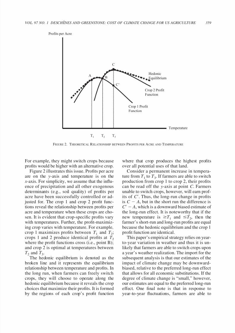
Figure 2 illustrates this issue. Profits per acre
are on the y-axis and temperature is on the x -axis. For simplicity, we assume that the influ-ence of precipitation and all other exogenousdeterminants (e.g., soil quality) of profits peracre have been successfully controlled or ad-
justed for. The crop 1 and crop 2 profit func-tions reveal the relationship between profits peracre and temperature when these crops are cho-sen. It is evident that crop-specific profits varywith temperatures. Further, the profit-maximiz-ing crop varies with temperature. For example,
crop 1 maximizes profits between T 1 and T 2;crops 1 and 2 produce identical profits at T 2
where the profit functions cross (i.e., point B);and crop 2 is optimal at temperatures betweenT 2
and T 3.
The hedonic equilibrium is denoted as thebroken line and it represents the equilibriumrelationship between temperature and profits. Inthe long run, when farmers can freely switchcrops, they will choose to operate along thehedonic equilibrium because it reveals the cropchoices that maximize their profits. It is formedby the regions of each crop’s profit function
where that crop produces the highest profitsover all potential uses of that land.
Consider a permanent increase in tempera-
ture from T 1 to T 3. If farmers are able to switchproduction from crop 1 to crop 2, their profitscan be read off the y-axis at point C . Farmersunable to switch crops, however, will earn prof-its of C . Thus, the long-run change in profitsis C A, but in the short run the difference isC A, which is a downward biased estimate of the long-run effect. It is noteworthy that if thenew temperature is T
1 and T
2, then the
farmer’s short-run and long-run profits are equalbecause the hedonic equilibrium and the crop 1
profit function are identical.This paper’s empirical strategy relies on year-to-year variation in weather and thus it is un-likely that farmers are able to switch crops upona year’s weather realization. The import for thesubsequent analysis is that our estimates of theimpact of climate change may be downward-biased, relative to the preferred long-run effectthat allows for all economic substitutions. If thedegree of climate change is “small,” however,our estimates are equal to the preferred long-runeffect. One final note is that in response toyear-to-year fluctuations, farmers are able to
Temperature
Profits per Acre
T1 T2 T3
Crop 1 Profit
Function
B
C
A
Crop 2 Profit
Function
Hedonic
Equilibrium
C’
FIGURE 2. THEORETICAL RELATIONSHIP BETWEEN PROFITS PER ACRE AND TEMPERATURE
359VOL. 97 NO. 1 DESCHE ˆ NES AND GREENSTONE: COST OF CLIMATE CHANGE FOR US AGRICULTURE

7/18/2019 The economic impact of climate change
http://slidepdf.com/reader/full/the-economic-impact-of-climate-change 7/32
adjust their mix of inputs (e.g., fertilizer andirrigated water usage), so the subsequent esti-mates are preferable to production function es-timates that do not allow for any adaptation.
II. Data Sources and Summary Statistics
To implement the analysis, we collected themost detailed and comprehensive data availableon agricultural production, temperature, precip-itation, and soil quality. This section describesthe data and reports some summary statistics.
A. Data Sources
Agricultural Production.—The data on agri-
cultural production come from the 1978, 1982,1987, 1992, 1997, and 2002 Census of Agricul-ture. The operators of all farms and ranchesfrom which $1,000 or more of agricultural prod-ucts are produced and sold, or normally wouldhave been sold, during the census year are re-quired to respond to the census forms. For con-fidentiality reasons, counties are the finestgeographic unit of observation in these data.
In much of the subsequent regression analy-sis, county-level agricultural profits per acre of farmland is the dependent variable. The numer-
ator is constructed as the difference between themarket value of agricultural products sold andtotal production expenses across all farms in acounty. The production expense informationwas not collected in 1978 or 1982, so the 1987,1992, 1997, and 2002 data are the basis for theanalysis. The denominator includes acres de-voted to crops, pasture, and grazing. The reve-nues component measures the gross marketvalue before taxes of all agricultural productssold or removed from the farm, regardless of
who received the payment. It does not includeincome from participation in federal farm pro-grams,6 labor earnings off the farm (e.g., in-come from harvesting a different field), ornonfarm sources. Thus, it is a measure of therevenue produced with the land.
Total production expenses are the measure of costs. It includes expenditures by landowners,
contractors, and partners in the operation of thefarm business. It covers all variable costs (e.g.,seeds, labor, and agricultural chemicals/fertiliz-ers). It also includes measures of interest paidon debts and the amount spent on repair and
maintenance of buildings, motor vehicles, andfarm equipment used for farm business. Its chief limitation is that it does not account for therental rate of the portion of the capital stock thatis not secured by a loan, so it is only a partialmeasure of farms’ cost of capital. Just as withthe revenue variable, the measure of expenses islimited to those incurred in the operation of thefarm so, for example, any expenses associatedwith contract work for other farms is excluded.7
This measure of profits per acre is a substitute
for the ideal measure of total rent per acre, so itis instructive to compare the two. Since separateinformation on rental land is unavailable in theCensuses, we used tabulations from the 1999Agricultural Economics and Land OwnershipSurvey to estimate the mean rent per acre (cal-culated as the “cash rent for land, buildings, andgrazing” divided by the “acres rented withcash”8) as roughly $35 (2002$). The mean of agricultural profits per acre in the census sam-ple is about $42 (2002$), so agricultural prof-its per acre appear to overstate the rental rate
modestly. Consequently, it may be appropriateto multiply the paper’s estimates of the impactof climate change on profits by 0.83 (i.e., theestimated ratio of rent to profits) to obtain awelfare measure.
In our replication of the hedonic approach,we utilize the variable on the value of land andbuildings as the dependent variable. This vari-able is available in all six Censuses.
6 An exception is that it includes receipts from placingcommodities in the Commodity Credit Corporation loanprogram. These receipts differ from other federal paymentsbecause farmers receive them in exchange for products.
7 The Censuses contain separate variables for subcatego-ries of revenue (e.g., revenues due to crops and dairy sales),but expenditures are not reported separately for these dif-ferent types of operations. Consequently, we cannot provideseparate measures of profits by these categories, and insteadfocus on total agriculture profits.
8 The estimate of acres rented with cash includes someacres where the rent is a combination of cash and a share of the output. Consequently, the measure of rental rate per acreis an underestimate, because the cash rent variable does notaccount for the value of payments in crops. Barrett E.Kirwan (2005) reports that among rental land where at leastpart of the rent is paid in cash, roughly 85 percent of therental contracts are all cash, with the remainder constitutingcash/output share combinations. The point is that this down-ward bias is unlikely to be substantial.
360 THE AMERICAN ECONOMIC REVIEW MARCH 2007
7/18/2019 The economic impact of climate change
http://slidepdf.com/reader/full/the-economic-impact-of-climate-change 8/32
Finally, we use the census data to examinethe relationship between the yields of the twomost important crops (i.e., corn for grain andsoybeans) and annual weather fluctuations.Crop yields are measured as total bushels of
production per acres planted.
Soil Quality Data.—No study of agriculturalproductivity would be complete without data onsoil quality, and we rely on the National Re-source Inventory (NRI) for our measures of these variables. The NRI is a massive survey of soil samples and land characteristics fromroughly 800,000 sites which is conducted incensus years. We follow the convention in theliterature and use a number of soil quality vari-
ables as controls in the equations for land val-ues, profits, and yields, including measures of susceptibility to floods, soil erosion (K-Factor),slope length, sand content, irrigation, and per-meability. County-level measures are calculatedas weighted averages across sites used for agri-culture, where the weight is the amount of landthe sample represents in the county. Althoughthese data provide a rich portrait of soil quality,we suspect that they are not comprehensive.Our approach is motivated by this possibility of unmeasured soil quality and other determinants
of productivity.
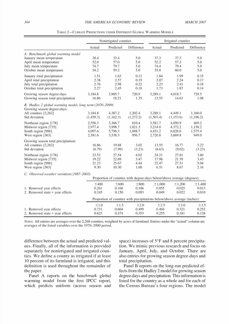
Climate and Weather Data.—The climatedata are derived from the Parameter-ElevationRegressions on Independent Slopes Model(PRISM).9 This model generates estimates of precipitation and temperature at 4 4 kilometergrid cells for the entire United States. The datathat are used to derive these estimates are fromthe National Climatic Data Center’s Summaryof the Month Cooperative Files. The PRISM
model is used by NASA, the Weather Channel,and almost all professional weather services. Itis regarded as one of the most reliable interpo-lation procedures for climatic data on a smallscale.
This model and data are used to developmonth-by-year measures of precipitation andtemperature for the agricultural land in each
county for the 1970–2000 period. This wasaccomplished by overlaying a map of land useson the PRISM predictions for each grid cell andthen by taking the simple average across allagricultural land grid cells. To replicate the
previous literature’s application of the hedo-nic approach, we calculated the climate nor-mals as the simple average of each county’smonthly estimates of temperature and precip-itation for each year between 1970 and twoyears before the relevant census year. Fur-thermore, we follow the convention in theliterature and include the January, April, July,and October mean as independent variables inthe analysis (Mendelsohn, Nordhaus, and Shaw1994, 1999; SHF 2005).
Although the monthly averages may be ap-propriate for a hedonic analysis of propertyvalues, there are better methods for modelingthe effect of weather on annual agriculturalprofits. Agronomists have shown that plantgrowth depends on the cumulative exposureto heat and precipitation during the growingseason. The standard agronomic approach formodeling temperature is to convert daily tem-peratures into degree-days, which representheating units (Thomas Hodges 1991; WilliamGrierson 2002). The effect of heat accumulation
is nonlinear since temperature must be above athreshold for plants to absorb heat and below aceiling as plants cannot absorb extra heat whentemperature is too high. These thresholds orbases vary across crops, but we join SHF (2006)and follow J. T. Ritchie and D. S. NeSmith’s(1991) suggested characterization for the entireagricultural sector and use a base of 46.4° Fahr-enheit (F) and a ceiling of 89.6°F (or 8° and 32°Celsius (C)). Ritchie and NeSmith also discussthe possibility of a temperature threshold at
93.2°F (34°C), above which increases in tem-perature are harmful. We explore this possibil-ity below.
We use daily-level data on temperatures tocalculate growing season degree-days betweenApril 1 and September 30. This period coversthe growing season for most crops, except win-ter wheat (USDA National Agriculture Statis-tics Service (NASS) 1997). The degree-daysvariable is calculated so that a day with a meantemperature below 46.4°F contributes 0 degree-days; between 46.4°F and 89.6°F contributesthe number of degrees above 46.4 degree-days;
9 PRISM was developed by the Spatial Climate AnalysisService at Oregon State University for the National Oceanicand Atmospheric Administration. See http://www.ocs.orst.edu/prism/docs/przfact.html for further details.
361VOL. 97 NO. 1 DESCHE ˆ NES AND GREENSTONE: COST OF CLIMATE CHANGE FOR US AGRICULTURE

7/18/2019 The economic impact of climate change
http://slidepdf.com/reader/full/the-economic-impact-of-climate-change 9/32
above 89.6°F contributes 43.2 degree-days. Thegrowing season degree-day variable is then cal-culated by summing the daily measures over theentire growing season.
Unfortunately, the monthly PRISM data can-
not be used to directly develop a measure of growing season degree-days. To measure thesedegree-day variables, we used daily-level dataon mean daily temperature from the approxi-mately 8,000 operational weather stations lo-cated in the United States during our sampleperiod. These data were obtained from the Na-tional Climatic Data Center “Cooperative Sum-mary of the Day” files. The construction of thesample used is described with more detail in theAppendix. Our use of daily data to calculate
degree-days is an important improvement overprevious work that has estimated growing sea-son degree-days with monthly data and distri-butional assumptions (H. C. S. Thom 1966;SHF 2006). Finally, in the specifications thatuse the degree-day measures of temperature, theprecipitation variable is total precipitation in thegrowing season, which is measured with thePRISM data as the sum of precipitation acrossthe growing season months in the relevant year.
Climate Change Predictions.—We rely on
two sets of predictions about climate change todevelop our estimates of its effects on US agri-cultural land. The first predictions rely on theclimate change scenario from the first Intergov-ernmental Panel on Climate Change (IPCC) re-port associated with a doubling of atmosphericconcentrations of greenhouse gases by the endof the twenty-first century (IPCC 1990; Na-tional Academy of Sciences 1991). This modelassumes uniform increases (across months andregions of the United States and their interac-
tion) of 5°F in temperature and 8 percent inprecipitation and has been used extensively inthe previous literature (Mendelsohn, Nordhaus,and Shaw 1994, 1999; SHF 2005).
The second set of predictions is from the Had-ley Centre’s Second Coupled Ocean-AtmosphereGeneral Circulation Model, which we refer to asHadley 2 (T. C. Johns et al. 1997). This modelof climate is comprised of several individuallymodeled components—the atmosphere, theocean, and sea ice—which are equilibrated us-ing a “spinup” process. The Hadley 2 model andan emissions scenario are used to obtain daily
state-level predictions for January 1994 throughDecember 2099. The emissions scenario as-sumes a 1-percent compounded increase peryear in both carbon dioxide and IS92A sulphateaerosols, which implies an increase in green-
house gas concentrations to roughly 2.5 timescurrent levels by the end of the twenty-firstcentury. This emissions assumption is standardand the climate change prediction is in the mid-dle of the range of predictions. From these dailypredictions, we calculate predicted growing sea-son degree-days and total precipitation usingthe formulas described above (see the DataAppendix (http://www.e-aer.org/data/mar07/ 20040638_data.zip) for further details).10 Wefocus on the “medium-term” and “long-run” ef-
fects on climate, which are defined as averages of growing season degree-days and precipitationover the 2020–2049 and 2070–2099 periods.
B. Summary Statistics
Agricultural Finances, Soil, and Weather Statistics.—Table 1 reports county-level sum-mary statistics from the three data sources for1978, 1982, 1987, 1992, 1997, and 2002. Thesample comprises a balanced panel of 2,268counties.11 Over the period, the number of
farms per county varied between 680 and 800.The total number of acres devoted to farmingdeclined by roughly 7.5 percent. At the sametime, the acreage devoted to cropland wasroughly constant, implying that the declinewas due to reduced land for livestock, dairy,and poultry farming. The mean average valueof land and buildings per acre ranged between$892 and $1,370 (2002$), with the peak and
10 The Hadley Centre has released a third climate model,which has some technical improvements over the second.We do not use it for this paper’s predictions, because dailypredictions are not yet available on a subnational scale overthe course of the entire twenty-first century to make state-level predictions about climate.
11 Observations from Alaska and Hawaii were excluded.We also dropped all observations from counties that hadmissing values for one or more years on any of the soilvariables, acres of farmland, acres of irrigated farmland, percapita income, population density, and latitude at the countycentroid. The sample restrictions were imposed to provide abalanced panel of counties from 1978 to 2002 for thesubsequent regressions.
362 THE AMERICAN ECONOMIC REVIEW MARCH 2007

7/18/2019 The economic impact of climate change
http://slidepdf.com/reader/full/the-economic-impact-of-climate-change 10/32
trough occurring in 1978 and 1992, respec-tively.12 (All subsequent figures are reported in2002 constant dollars, unless noted otherwise.)
The second panel details annual financial in-formation about farms. We focus on the 1987–2002 period, since complete data are availableonly for these four censuses. During this period,the mean county-level sales of agriculturalproducts ranged from $72 million to $80 mil-lion. Although it is not reported here, the shareof revenue from crop products increased from
43.7 percent to 47.9 percent in this period, withthe remainder coming from the sale of livestock and poultry. Farm production expenses grewfrom $57 million to $65 million. The meancounty profits from farming operations were$14.4 million, $14.0 million, $18.6 million,$10.0 million, or $42, $41, $56, and $30 peracre in 1987, 1992, 1997, and 2002, respec-
tively. These profit figures do not include gov-ernment payments, which are listed at thebottom of this panel. The subsequent analysis of profits also excludes government payments.
The third panel lists the means of the avail-able measures of soil quality, which are keydeterminants of lands’ productivity in agricul-ture. These variables are essentially unchangedacross years since soil and land types at a givensite are generally time-invariant. The smalltime-series variation is due to changes in the
composition of land that is used for farming.Notably, the only measure of salinity is from1982, so we use this measure for all years.
Climate Change Statistics.—Panels A and Bof Table 2 report on the predictions of twoclimate change models. All entries are calcu-lated as the weighted average across the fixedsample of 2,268 counties, where the weight isthe number of acres of farmland. The “Actual”column shows the 1970–2000 averages of eachof the listed variables. There are also columnsfor the predicted values of the variables and the
12 All entries are simple averages over the 2,268 counties,except “Average Value of Land/Bldg (1$/acre)” and “Profitper Acre (1$/acre),” which are weighted by acres of farmland.
TABLE 1—COUNTY-LEVEL SUMMARY STATISTICS
1978 1982 1987 1992 1997 2002
FARMLAND AND ITS VALUE
Number of farms 799.3 796.3 745.4 688.3 684.9 766.5
Land in farms (th. acres) 363.7 352.4 345.5 338.4 333.4 336.1Total cropland (th. acres) 158.7 156.0 158.3 155.9 154.1 155.3Avg. value of land & buildings ($1/acre) 1,370.4 1,300.7 907.3 892.2 1,028.2 1,235.6Avg. value of machinery & equipment ($1/acre) — — 126.7 118.8 129.2 145.8ANNUAL FINANCIAL INFORMATION
Profits ($mil.) — — 14.4 14.0 18.6 10.0Profits per acre ($1/acre) — — 41.7 41.3 55.7 29.7Farm revenues ($mil.) 88.7 80.0 71.5 72.9 79.9 74.9Total farm expenses ($mil.) — — 57.2 58.9 61.3 64.9Total government payments ($mil.) — — 4.8 2.3 1.9 2.4MEASURES OF SOIL PRODUCTIVITY
K-Factor 0.30 0.30 0.30 0.30 0.30 0.30Slope length 218.9 218.9 218.3 217.8 218.3 218.3Fraction flood-prone 0.15 0.15 0.15 0.15 0.15 0.15
Fraction sand 0.09 0.09 0.09 0.09 0.09 0.09Fraction clay 0.18 0.18 0.18 0.18 0.18 0.18Fraction irrigated 0.18 0.18 0.18 0.18 0.19 0.19Permeability 2.90 2.90 2.90 2.88 2.88 2.88Moisture capacity 0.17 0.17 0.17 0.17 0.17 0.17Wetlands 0.10 0.10 0.10 0.10 0.10 0.10Salinity 0.01 0.01 0.01 0.01 0.01 0.01
Notes: Averages are calculated for a balanced panel of 2,268 counties. All entries are simple averages over the 2,268 counties,with the exception of “average value of land & buildings (1$/acre)” and “profit per acre (1$/acre),” which are weighted byacres of farmland. All dollar values are in 2002 constant dollars.
363VOL. 97 NO. 1 DESCHE ˆ NES AND GREENSTONE: COST OF CLIMATE CHANGE FOR US AGRICULTURE
7/18/2019 The economic impact of climate change
http://slidepdf.com/reader/full/the-economic-impact-of-climate-change 11/32
difference between the actual and predicted val-ues. Finally, all of the information is providedseparately for nonirrigated and irrigated coun-ties. We define a county as irrigated if at least10 percent of its farmland is irrigated, and thisdefinition is used throughout the remainder of the paper.
Panel A reports on the benchmark globalwarming model from the first IPCC report,which predicts uniform (across season and
space) increases of 5°F and 8 percent precipita-tion. We mimic previous research and focus onJanuary, April, July, and October. There arealso entries for growing season degree-days andtotal precipitation.
Panel B reports on the long-run predicted ef-fects from the Hadley 2 model for growing seasondegree-days and precipitation. This information islisted for the country as a whole and for each of the Census Bureau’s four regions. The model
TABLE 2—CLIMATE PREDICTIONS UNDER DIFFERENT GLOBAL WARMING MODELS
Nonirrigated counties Irrigated counties
Actual Predicted Difference Actual Predicted Difference
A. Benchmark global warming modelJanuary mean temperature 28.4 33.4 5.0 32.3 37.3 5.0April mean temperature 52.0 57.0 5.0 52.2 57.2 5.0July mean temperature 74.7 79.7 5.0 74.4 79.4 5.0October mean temperature 54.2 59.2 5.0 55.0 60.0 5.0
January total precipitation 1.51 1.63 0.12 1.84 1.99 0.15April total precipitation 2.38 2.57 0.19 2.07 2.24 0.17July total precipitation 2.76 2.98 0.22 2.23 2.41 0.18October total precipitation 2.27 2.45 0.18 1.73 1.87 0.14
Growing season degree-days 3,184.8 3,905.7 720.9 3,289.1 4,018.7 729.5Growing season total precipitation 16.86 18.21 1.35 13.55 14.63 1.08
B. Hadley 2 global warming model, long term (2070–2099)Growing season degree-days:
All counties [2,262] 3,184.8 4,387.2 1,202.4 3,289.1 4,449.1 1,160.0Std deviation (1,459.3) (1,162.3) (1,272.2) (1,503.4) (1,153.6) (1,196.2)
Northeast region [178] 2,556.3 3,366.7 810.4 3,581.7 4,050.9 469.2Midwest region [735] 2,977.4 3,998.7 1,021.3 3,214.0 4,372.2 1,158.2South region [986] 4,097.6 5,796.3 1,698.7 4,451.2 6,026.6 1,575.4West region [363] 2,581.6 3,538.3 956.7 2,720.8 3,669.8 949.0
Growing season total precipitation:All counties [2,262] 16.86 19.88 3.02 13.55 16.77 3.22Std deviation (6.79) (7.99) (3.23) (8.63) (9.02) (3.23)
Northeast region [178] 23.52 27.54 4.02 24.21 27.81 3.60Midwest region [735] 19.22 22.69 3.47 17.96 21.39 3.43South region [986] 21.23 25.67 4.44 22.47 27.51 5.04West region [363] 9.30 10.30 1.00 6.51 8.67 2.16
C. Observed weather variation (1987–2002)Proportion of counties with degree-days below/above average (degrees):
400 600 800 1,000 1,200 1,4001. Removed year effects 0.261 0.166 0.106 0.055 0.025 0.0132. Removed state year effects 0.245 0.150 0.093 0.049 0.022 0.010
Proportion of counties with precipitations below/above average (inches):
1.0 1.5 2.0 2.5 3.0 3.51. Removed year effects 0.731 0.604 0.499 0.404 0.321 0.2522. Removed state year effects 0.623 0.474 0.353 0.255 0.181 0.128
Notes: All entries are averages over the 2,268 counties, weighted by acres of farmland. Entries under the “actual” column are
averages of the listed variables over the 1970–2000 period.
364 THE AMERICAN ECONOMIC REVIEW MARCH 2007

7/18/2019 The economic impact of climate change
http://slidepdf.com/reader/full/the-economic-impact-of-climate-change 12/32
predicts a mean increase in degree-days of roughly 1,200 by the end of the century (i.e., the2070 –2099 period). The most striking regionaldifference is the dramatic increase in temperaturein the South. Its long-run predicted increase in
degree-days of roughly 1,700 among nonirrigatedcounties greatly exceeds the approximate in-creases of 810, 1,000, and 960 degree-days in theNortheast, Midwest, and West, respectively. Theoverall average increase in growing season pre-cipitation in the long run is approximately 3.0inches, with the largest predicted increase inthe South and smallest increase in the West.There is also substantial intraregional (e.g., atthe state level) variation in the climate changepredictions, and this variation is used in the
remainder of the paper to infer the economicimpacts of climate change.
Weather Variation Statistics.—In our pre-ferred approach, we aim to infer the effects of weather fluctuations on agricultural profits. Wefocus on regression models that include countyand year fixed effects and county and state byyear fixed effects. It would be ideal if, afteradjustment for these fixed effects, the variationin the weather variables that remains is as largeas those predicted by the climate change models
used in this study. In this case, our predictedeconomic impacts will be identified from thedata, rather than by extrapolation due to func-tional form assumptions.
Panel C reports on the magnitude of the de-viations between counties’ yearly weather real-izations and their long-run averages after takingout year (row 1) and state by year fixed effects(row 2). Therefore, it provides an opportunity toassess the magnitude of the variation in growingseason degree-days and precipitation after ad-
justment for permanent county factors (e.g.,whether the county is usually hot or wet) andnational time varying factors (e.g., whether itwas a hot or wet year nationally) or state-spe-cific, time-varying factors (e.g., whether it wasa hot or wet year in a particular state).
Specifically, the entries report the fraction of county by year observations with deviations atleast as large as the one reported in the columnheading, averaged over the years 1987, 1992,1997, and 2002. For example, the “RemovedState Year Effects” degree-days row indicatethat 24.5 percent, 9.3 percent, and 2.2 percent of
county by year observations had deviationslarger than 400, 800, and 1,200 degree-days,respectively. The corresponding row for grow-ing season precipitation reports that 62.3 per-cent, 35.3 percent, and 18.1 percent of the
county by year observations had deviationslarger than 1.0, 2.0, and 3.0 inches, respectively.
Temperature and precipitation deviations of the magnitudes predicted by the climate changemodels occur in the data. This is especially trueof precipitation where more than 18 percent of county by year observations have a deviationlarger than 3.0 inches, which roughly equals thepredicted increase from the long-run Hadley 2scenario. The impact of the scenario’s meanincrease of about 1,200 degree-days could be
nonparametrically identified, although it wouldcome from just 2.2 percent of observations.However, 5 percent of annual county observa-tions have deviations as large as 1,000 degree-days. Finally, it is noteworthy that differencingout state weather shocks does not substantiallyreduce the frequency of large deviations, high-lighting that there are important regional pat-terns to weather shocks.
III. Econometric Strategy
A. The Hedonic Approach
This section describes the econometricframework that we use to assess the conse-quences of global climate change. We initiallyconsider the hedonic cross-sectional model thathas been predominant in the previous literature(Mendelsohn, Nordhaus, and Shaw 1994, 1999;SHF 2005, 2006). Equation (3) provides a stan-dard formulation of this model:
(3) yct X ct ii f iW ic ct
ct c uct ,
where yct is the value of agricultural land peracre in county c in year t . The t subscript indi-cates that this model could be estimated in anyyear for which data are available. X ct is a vectorof observable determinants of farmland values,some of which are time-varying. The last termin equation (3) is the stochastic error term, ct ,
365VOL. 97 NO. 1 DESCHE ˆ NES AND GREENSTONE: COST OF CLIMATE CHANGE FOR US AGRICULTURE
7/18/2019 The economic impact of climate change
http://slidepdf.com/reader/full/the-economic-impact-of-climate-change 13/32
which comprises a permanent, county-specificcomponent, c, and an idiosyncratic shock, uct .W ic represents a series of climate variables
for county c. We follow Mendelsohn, Nor-dhaus, and Shaw (1994) and let i indicate one of
eight climatic variables. In particular, there areseparate measures of temperature and total pre-cipitation in January, April, July, and October,so there is one month from each quarter of theyear. The appropriate functional form for eachof the climate variables is unknown, but in ourreplication of the hedonic approach, we followthe convention in the literature and model theclimatic variables with linear and quadraticterms. As emphasized by SHF (2005), it isimportant to allow the effect of climate to differ
across nonirrigated and irrigated counties. Ac-cordingly, we include interactions of all theclimate variables and indicators for nonirrigatedand irrigated counties.
The coefficient vector is the “true” effect of climate on farmland values and its estimates areused to calculate the overall effect of climatechange associated with the benchmark 5°F in-crease in temperature and 8 percent increase inprecipitation. Since the total effect of climatechange is a linear function of the components of the vector, it is straightforward to formulate
and implement tests of the effects of alternativeclimate change scenarios on agricultural landvalues.13 We will report the standard errorsassociated with the overall estimate of the effectof climate change. The total effect of climatechange, however, is a function of 32 parameterestimates when the climate variables are mod-eled with a quadratic, so it is not surprising thatstatistical significance is elusive.
Consistent estimation of the vector , andconsequently of the effect of climate change,
requires that E[ f i(W ic)ct X ct ] 0 for each cli-mate variable i. This assumption will be invalidif there are unmeasured permanent (c) and/ortransitory (uct ) factors that covary with the climatevariables. To obtain reliable estimates of , wecollected a wide range of potential explanatory
variables, including all the soil quality variableslisted in Table 1, as well as per capita income andpopulation density.14 We also estimate spec-ifications that include state fixed effects.
There are three further issues about equation
(3) that bear noting. First, it is likely that theerror terms are correlated among nearby geo-graphical areas. For example, unobserved soilproductivity is spatially correlated, so the stan-dard OLS formulas for inference are likely in-correct. In the absence of knowledge on thesources and the extent of residual spatial depen-dence in land value data, we adjust the standarderrors for spatial dependence of an unknownform following the approach of Timothy G.Conley (1999). The basic idea is that the spatial
dependence between two observations will de-cline as the distance between the counties in-creases.15 Throughout the paper, we presentstandard errors calculated with the Eicker-White formula that allows for heteroskedastic-ity of an unspecified nature. In addition, wepresent the Conley standard errors for our pre-ferred fixed-effect models.
Second, it may be appropriate to weight equa-tion (3). Since the dependent variable is county-level farmland values per acre, we think there aretwo complementary reasons to weight by the
square root of acres of farmland. First, the esti-mates of the value of farmland from counties withlarge agricultural operations will be more precisethan the estimates from counties with small oper-ations, and this weight corrects for the heteroske-dasticity associated with the differences in precision.Second, the weighted mean of the dependent vari-able is equal to the mean value of farmland peracre in the country.
13 Since we use a quadratic model for the climate vari-ables, each county’s predicted impact is calculated as thediscrete difference in agricultural land values at the county’spredicted temperatures and precipitation after climatechange and its current climate (i.e., the average over the1970–2000 period).
14 Previous research suggests that urbanicity, populationdensity, the local price of irrigation, and air pollution con-centrations are important determinants of land values (Wil-liam R. Cline 1996; Andrew Plantinga, Ruben Lubowski,and Robert Stavins 2002; SHF 2005, 2006; Chay andGreenstone 2005). Comprehensive data on the price of irrigation and air pollution concentrations are unavailable.
15 More precisely, the Conley (1999) covariance matrixestimator is obtained by taking a weighted average of spatialautocovariances. The weights are given by the product of Bartlett kernels in two dimensions (north/south and east/ west), which decline linearly from 1 to 0. The weights reach0 when one of the coordinates exceeds a prespecified cutoff point. Throughout, we choose the cutoff points to be 7degrees of latitude and longitude, corresponding to dis-tances of about 500 miles.
366 THE AMERICAN ECONOMIC REVIEW MARCH 2007

7/18/2019 The economic impact of climate change
http://slidepdf.com/reader/full/the-economic-impact-of-climate-change 14/32
Mendelsohn, Nordhaus, and Shaw (1994,1999) and SHF (2005) use the square root of thepercent of the county in cropland and the squareroot of total revenue from crop sales as weights.We elected not to report the results based on these
approaches in the main tables, since the motiva-tion for these weighting schemes is less transpar-ent. For example, it is difficult to justify theassumptions about the variance-covariance matrixthat would motivate these weights as a solution toheteroskedasticity. Further, although these weightsemphasize the counties that are most important tototal agricultural production, they do so in an uncon-ventional manner.
B. A New Approach
One of this paper’s primary points is that thecross-sectional hedonic equation is likely to bemisspecified. As a possible solution to thisproblem, we fit
(4) yct c t X ct i
i f iW ict uct .
There are a number of important differencesbetween equations (4) and (3). For starters,equation (4) includes a full set of county fixed
effects, c. The appeal of including the countyfixed effects is that they absorb all unobservedcounty-specific time invariant determinants of the dependent variable.16 The equation also in-cludes year indicators, t , that control for annualdifferences in the dependent variable that arecommon across counties. Our preferred specifi-cation replaces the year fixed effects with stateby year fixed effects ( st ).
The inclusion of the county fixed effects ne-cessitates two substantive differences in equa-
tion (4), relative to (3). First, the dependentvariable, yct , is now county-level agriculturalprofits, instead of land values.17 This is because
land values capitalize long-run characteristicsof sites and, conditional on county fixed effects,annual realizations of weather should not affectland values. Weather does, however, affect farmrevenues and expenditures and their difference
is equal to profits.Second, it is impossible to estimate the effect
of the long-run climate averages in a model withcounty fixed effects, because there is no tempo-ral variation in W ic. Consequently, we replacethe climate variables with annual realizations of weather, W ict . We follow the standard agro-nomic approach and model temperature by us-ing growing season degree-days, defined with abase of 46.4°F and a ceiling of 89.6°F. Simi-larly, we model the effect of precipitation on
agricultural profits per acre by using growingseason precipitation. Once again, we let theeffects of these variables differ across irrigatedand nonirrigated counties. Further, we modelthem with quadratics.
The validity of any estimate of the impact of climate change based on equation (4) rests cru-cially on the assumption that its estimation willproduce unbiased estimates of the vector.Formally, the consistency of each i requiresE[ f i(W ict )uct X ct , c, st ] 0. By conditioningon the county and state by year fixed effects, the
i’s are identified from county-specific devia-tions in weather about the county averages aftercontrolling for shocks common to all countiesin a state. This variation is presumed to beorthogonal to unobserved determinants of agri-cultural profits, so it provides a potential solu-tion to the omitted variables bias problems thatappear to plague the estimation of equation (3).A shortcoming of this approach is that all thefixed effects are likely to magnify the impor-tance of misspecification due to measurement
error, which generally attenuates the estimatedparameters.
IV. Results
This section is divided into three subsec-tions. The first provides some suggestive ev-idence on the validity of the hedonic approach
16 Interestingly, the fixed-effects model was first devel-oped by Hoch (1958, 1962) and Mundlak (1961) to accountfor unobserved heterogeneity in estimating farm productionfunctions.
17 Similarly, Kelly, Kolstad, and Mitchell (2005) esti-mate the cross-sectional relationship between agriculturalprofits and weather realizations for a sample of five USstates (Illinois, Iowa, Kansas, Missouri, and Nebraska).However, they control for climate variables rather thancounty fixed effects so their approach is more restrictive
than the one we use in this paper. Nevertheless their esti-mated impact of climate change on agricultural profits (inpercentage terms) is similar to ours.
367 VOL. 97 NO. 1 DESCHE ˆ NES AND GREENSTONE: COST OF CLIMATE CHANGE FOR US AGRICULTURE
7/18/2019 The economic impact of climate change
http://slidepdf.com/reader/full/the-economic-impact-of-climate-change 15/32
and then presents results from that approach.The second subsection presents results fromthe fitting of equation (4) to estimate theimpact of climate change on the US agricul-tural sector. It also probes the distributionalconsequences of climate change across the
country. The third and final subsection esti-mates the effect of climate change on cropyields for corn for grain, and for soybeans, thetwo most important crops in the agriculturalsector in terms of value.
A. Estimates of the Impact of ClimateChanges from the Hedonic Approach
Does Climate Vary with Observables?—As
the previous section highlighted, the hedonicapproach relies on the assumption that the cli-mate variables are orthogonal to the unobserved determinants of land values. We begin by ex-amining whether these variables are orthogonalto observable predictors of farm values. Whilethis is not a formal test of the identifying as-sumption, there are at least two reasons that itmay seem reasonable to presume that this ap-proach will produce valid estimates of the ef-fects of climate when the observables arebalanced. First, consistent inference will notdepend on functional form assumptions on the
relation between the observable confoundersand farm values. Second, the unobservablesmay be more likely to be balanced (Joseph G.Altonji, Todd E. Elder, and Christopher R.Taber 2000).
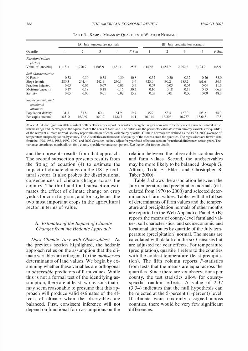
Table 3 shows the association between the
July temperature and precipitation normals (cal-culated from 1970 to 2000) and selected deter-minants of farm values. Tables with the full setof determinants of farm values and the temper-ature and precipitation normals of other monthsare reported in the Web Appendix. Panel A (B)reports the means of county-level farmland val-ues, soil characteristics, and socioeconomic andlocational attributes by quartile of the July tem-perature (precipitation) normal. The means arecalculated with data from the six Censuses but
are adjusted for year effects. For temperature(precipitation), quartile 1 refers to the countieswith the coldest temperature (least precipita-tion). The fifth column reports F -statisticsfrom tests that the means are equal across thequartiles. Since there are six observations percounty, the test statistics allow for county-specific random effects. A value of 2.37(3.34) indicates that the null hypothesis canbe rejected at the 5-percent (1-percent) level.If climate were randomly assigned acrosscounties, there would be very few significantdifferences.
TABLE 3—SAMPLE MEANS BY QUARTILES OF WEATHER NORMALS
Quartile
[A] July temperature normals [B] July precipitation normals
1 2 3 4 F -Stat 1 2 3 4 F -Stat
Farmland values
($1/ac)Value of land/bldg 1,118.3 1,770.7 1,608.9 1,481.1 25.5 1,149.6 1,458.9 2,252.2 2,194.7 148.9
Soil characteristicsK Factor 0.32 0.30 0.32 0.30 10.8 0.32 0.30 0.32 0.26 33.0Slope length 280.3 244.4 242.1 230.1 3.6 323.9 199.2 185.2 161.6 54.7Fraction irrigated 0.05 0.06 0.07 0.06 3.9 0.07 0.05 0.03 0.04 11.6Moisture capacity 0.17 0.18 0.18 0.15 50.7 0.16 0.18 0.19 0.15 106.9Salinity 0.05 0.03 0.01 0.02 15.8 0.05 0.01 0.00 0.00 48.0
Socioeconomic and
locational
attributesPopulation density 31.3 83.8 60.1 64.9 19.7 35.9 53.4 127.0 108.2 54.0Per capita income 16,510 16,369 16,017 14,847 14.1 16,014 16,206 16,777 15,043 17.3
Notes: All dollar figures in 2002 constant dollars. The entries report the results of weighted regressions where the dependent variable is noted in therow headings and the weight is the square root of the acres of farmland. The entries are the parameter estimates from dummy variables for quartilesof the relevant climate normal, so they report the mean of each variable by quartile. Climate normals are defined as the 1970–2000 average of temperature and precipitation, by county. The F -statistics are from tests of equality of the means across the quartiles. The regressions are fit with datafrom the 1978, 1982, 1987, 1992, 1997, and 2002 Censuses, so they adjust for year fixed effects to account for national differences across years. Thevariance-covariance matrix allows for a county-specific variance component. See the text for further details.
368 THE AMERICAN ECONOMIC REVIEW MARCH 2007

7/18/2019 The economic impact of climate change
http://slidepdf.com/reader/full/the-economic-impact-of-climate-change 16/32
It is immediately evident that the observabledeterminants of farmland values are not bal-anced across the quartiles of weather normals:all of the F -statistics markedly reject the nullhypothesis of equality across quartiles. In fact,
in our extended analysis reported in the WebAppendix, the null hypothesis of equality of thesample means of the explanatory variablesacross quartiles can be rejected at the 1-percentlevel in 111 of the 112 cases considered.18
In many cases the differences in the meansare large, implying that rejection of the null isnot simply due to the sample sizes. For exam-ple, the fraction of the land that is irrigated andthe population density (a measure of urbanicityor of the likelihood of conversion to residential
housing) in the county are known to be impor-tant determinants of the agricultural land values,and their means vary dramatically across quar-tiles of the climate variables. In fact, the findingthat population density is associated with agri-cultural land values undermines the validity of the hedonic approach to learn about climatechange because density has no direct impact onagricultural yields. Overall, the entries suggestthat the conventional cross-sectional hedonicapproach may be biased due to incorrect spec-ification of the functional form of the observed
variables and potentially due to unobservedvariables.
Replication of the SHF (2005) Hedonic Ap- proach.—With these results in mind, we imple-ment the hedonic approach outlined in equation(3). We begin by replicating the analysis of SHF(2005) using their data based on the 1982 Cen-sus of Agriculture and their programs, both of which they provided. We follow their proposedapproach and use a quadratic in each of the
eight climate variables.Although the point of their paper is that pool-ing irrigated and nonirrigated counties can leadto biased estimates of climate parameters in
hedonic models, they report only those esti-mates based on specifications that constrain theeffect of climate to be the same in both sets of counties. Based on this approach, the aggregateimpact of the benchmark scenario increases of
5°F in temperatures and 8 percent in precipita-tion on farmland values is $543.7 billion(2002$) with cropland weights or $69.1 billionwith crop revenue weights. Except for a Con-sumer Price Index (CPI) adjustment, these esti-mates are identical to those in SHF (2005).
To probe the robustness of these results, wereestimate the hedonic models using two alterna-tive sets of covariates. The first drops all covari-ates, except the climate variables, while thesecond adds state fixed effects to the specification
used by SHF. The state fixed effects account forall unobserved differences across states (e.g., soilquality and state agricultural programs). The sim-ple specification that controls only for the climatevariables produces an estimate of $98.5 billionwith the cropland weights and $437.6 billion withthe crop revenue weights. The specification thatadds state fixed effects produces estimates of $477.8 billion and $1,034 billion. The latterfigure seems implausible, since it is nearly as largeas the entire value of agricultural land and build-ings in the United States, which was $1,115 bil-
lion in 2002.As discussed previously, our view is that
these two sets of weights have no clear justifi-cation. In our opinion, the appropriate approachis to weight by acres of farmland. Reestimationof the SHF, climate variables only, and SHFplus state fixed effects specifications with thereconstructed version of the SHF data file pro-duces estimates of $225.1 billion, $315.4 bil-lion, and $0.6 billion. Consequently, the SHFfindings also appear to be related to the choice
of weights. It seems reasonable to conclude thatthe application of the hedonic approach to theSHF data fails to produce robust estimates of the impact of climate change, even with a singleyear of data. In our view, the fragility or non-robustness of this approach is not conveyedadequately in their article or in Mendelsohn,Nordhaus, and Shaw (1994).19
18 We also divided the sample into nonirrigated andirrigated counties, where a county is defined as irrigated if at least 10 percent of the farmland is irrigated and the othercounties are labeled nonirrigated. Among the nonirrigated(irrigated) counties, the null hypothesis of equality of thesample means of the explanatory variables across quartilescan be rejected at the 1-percent level for 111 (96) of the 112covariates.
19 Among nonirrigated counties, the same set of esti-mates ranges from $144.2 billion to $396.2 billion, sothe same conclusion applies to nonirrigated counties as
369VOL. 97 NO. 1 DESCHE ˆ NES AND GREENSTONE: COST OF CLIMATE CHANGE FOR US AGRICULTURE

7/18/2019 The economic impact of climate change
http://slidepdf.com/reader/full/the-economic-impact-of-climate-change 17/32
New Hedonic Estimates.—Table 4 further in-vestigates the robustness of the hedonic ap-proach by conducting our own broader analysis.To this end, we assemble our samples from the
1978–2002 Censuses of Agriculture. We main-tain the same quadratic specification in each of the eight climate variables.
There are some important differences be-tween our approach and SHF. First, we fit re-gressions that allow the effects of climate onfarmland values to vary in irrigated and nonir-rigated counties. In addition, the regressions
allow for intercept differences across irrigatedand nonirrigated counties but constrain all otherparameters to be equal in the two sets of coun-ties. Second, we report standard errors for the
estimated impacts. Third, we do not truncate thecounty-specific estimated impacts at zero.The entries in Table 4 report the predicted
changes in land values in billions of 2002 dollars(and their standard errors in parentheses) from thebenchmark increases of five degrees Fahrenheitand 8 percent in precipitation. These predictedchanges are based on the estimated climate pa-rameters from the fitting of equation (3). The 42different estimates of the national impact on landvalues are the result of 7 different data samples, 3specifications, and 2 assumptions about the correctweights. The data samples are denoted in the row
well. Recent research, however, suggests that modelingtemperature with degree-days may reduce the variability of hedonic estimates (SHF 2006).
TABLE 4—HEDONIC ESTIMATES OF IMPACT OF BENCHMARK CLIMATE CHANGE SCENARIO ON AGRICULTURAL LAND VALUES
(IN BILLIONS OF 2002 DOLLARS), 1978–2002
Specification A B C
Weights (0) (1) (0) (1) (0) (1)
Single census year 1978 131.9 131.1 141.2 154.7 321.3 255.6
(35.6) (35.7) (38.0) (31.3) (46.1) (31.8)1982 36.3 36.1 19.2 40.8 203.3 154.6
(28.6) (25.7) (28.7) (24.4) (46.6) (32.2)1987 55.9 9.6 49.3 8.7 45.9 51.3
(25.8) (21.5) (27.5) (20.0) (38.8) (22.6)1992 50.4 23.0 32.9 8.1 22.3 46.4
(35.0) (31.6) (32.5) (24.5) (50.3) (25.2)1997 117.0 55.5 89.0 33.5 25.5 65.8
(32.7) (38.7) (35.3) (31.1) (46.5) (24.1)2002 288.6 139.5 202.1 101.0 8.8 60.9
(59.2) (61.4) (58.4) (49.5) (77.0) (38.7)
Pooled 1978–2002All counties 75.1 16.9 45.6 0.7 95.2 110.8
(28.0) (30.7) (30.6) (26.3) (41.6) (23.4)Nonirrigated counties 63.9 28.6 44.7 10.9 66.1 82.1
(24.3) (28.5) (28.0) (24.6) (35.5) (17.9)Irrigated counties 11.2 11.6 0.9 11.6 29.1 28.6
(13.7) (11.2) (12.2) (9.6) (13.1) (10.4)Soil variables No No Yes Yes Yes YesSocioecon. vars No No Yes Yes Yes YesState fixed-effects No No No No Yes Yes
Notes: All dollar figures in billions of 2002 constant dollars. The entries are the predicted impact on agricultural land valuesof the benchmark uniform increases of five degree Fahrenheit and 8 percent precipitation from the estimation of 56 differenthedonic models, noted as equation (3) in the text. The standard errors of the predicted impacts are reported in parentheses.
The 42 different sets of estimates of the national impact on land values are the result of seven different data samples, threespecifications, and two assumptions about the correct weights. The data samples are denoted in the row headings. There isa separate sample for each of the census years and the seventh is the result of pooling data from the six Censuses. Thespecification details are noted in the row headings at the bottom of the table. The weights used in the regressions are reportedin the top row and are as follows: (0) unweighted; (1) square root of acres of farmland. The estimated impacts are reportedseparately for nonirrigated and irrigated counties for the pooled sample. See the text for further details.
370 THE AMERICAN ECONOMIC REVIEW MARCH 2007
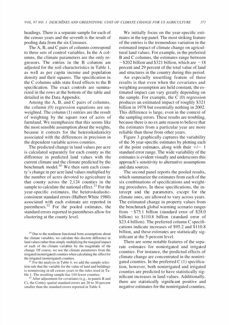
7/18/2019 The economic impact of climate change
http://slidepdf.com/reader/full/the-economic-impact-of-climate-change 18/32
headings. There is a separate sample for each of the census years and the seventh is the result of pooling data from the six Censuses.
The A, B, and C pairs of columns correspondto three sets of control variables. In the A col-
umns, the climate parameters are the only re-gressors. The entries in the B columns areadjusted for the soil characteristics in Table 1,as well as per capita income and populationdensity and their squares. The specification inthe C columns adds state fixed effects to the Bspecification. The exact controls are summa-rized in the rows at the bottom of the table anddetailed in the Data Appendix.
Among the A, B, and C pairs of columns,the column (0) regression equations are un-
weighted. The column (1) entries are the resultof weighting by the square root of acres of farmland. We reemphasize that this seems likethe most sensible assumption about the weights,because it corrects for the heteroskedasticityassociated with the differences in precision inthe dependent variable across counties.
The predicted change in land values per acreis calculated separately for each county as thedifference in predicted land values with thecurrent climate and the climate predicted by thebenchmark model.20 We then sum each coun-
ty’s change in per acre land values multiplied bythe number of acres devoted to agriculture inthat county across the 2,124 counties in thesample to calculate the national effect.21 For theyear-specific estimates, the heteroskedastic-consistent standard errors (Halbert White 1980)associated with each estimate are reported inparentheses.22 For the pooled estimates, thestandard errors reported in parentheses allow forclustering at the county level.
We initially focus on the year-specific esti-mates in the top panel. The most striking featureof the entries is the tremendous variation in theestimated impact of climate change on agricul-tural land values. For example, in the preferred
B and C columns, the estimates range between$202 billion and $321 billion, which are 18percent and 29 percent of the total value of landand structures in the country during this period.
An especially unsettling feature of theseresults is that even when the covariates andweighting assumption are held constant, the es-timated impact can vary greatly depending onthe sample. For example, the C (0) regressionproduces an estimated impact of roughly $321billion in 1978 but essentially nothing in 2002.
This difference is large, even in the context of the sampling errors. These results are troubling,because there is no ex ante reason to believe thatthe estimates from a particular year are morereliable than those from other years.
Figure 3 graphically captures the variabilityof the 36 year-specific estimates by plotting eachof the point estimates, along with their / 1standard error range. The wide variability of theestimates is evident visually and underscores thisapproach’s sensitivity to alternative assumptionsand data sources.
The second panel reports the pooled results,which summarize the estimates from each of thesix combinations of specifications and weight-ing procedures. In these specifications, the in-tercept and the parameters, except for theclimate ones, are allowed to vary across years.The estimated change in property values fromthe benchmark global warming scenario rangesfrom $75.1 billion (standard error of $28.0billion) to $110.8 billion (standard error of $23.4 billion). The preferred column C specifi-
cations indicate increases of $95.2 and $110.8billion, and these estimates are statistically sig-nificant at the 5-percent level.
There are some notable features of the sepa-rate estimates for nonirrigated and irrigatedcounties. For instance, the predicted effects of climate change are concentrated in the nonirri-gated counties. In the preferred C (1) specifica-tion, however, both nonirrigated and irrigatedcounties are predicted to have statistically sig-nificant increases in land values. Additionally,there are statistically significant positive andnegative estimates for the nonirrigated counties,
20 Due to the nonlinear functional form assumptions aboutthe climate variables, we calculate this discrete difference inland values rather than simply multiplying the marginal impactof each of the climate variables by the magnitude of thechange. Of course, we use the climate parameters from theirrigated (nonirrigated) counties when calculating the effect forthe irrigated (nonirrigated) counties.
21 For the analysis in Table 4, we add the sample selec-tion rule that the variable for the value of land and buildingsis nonmissing in all census years to the rules used in Ta-ble 1. The resulting sample has 144 fewer counties.
22 After adjustment for covariates (e.g., in panels B andC), the Conley spatial standard errors are 20 to 30 percentsmaller than the standard errors reported in Table 4.
371VOL. 97 NO. 1 DESCHE ˆ NES AND GREENSTONE: COST OF CLIMATE CHANGE FOR US AGRICULTURE
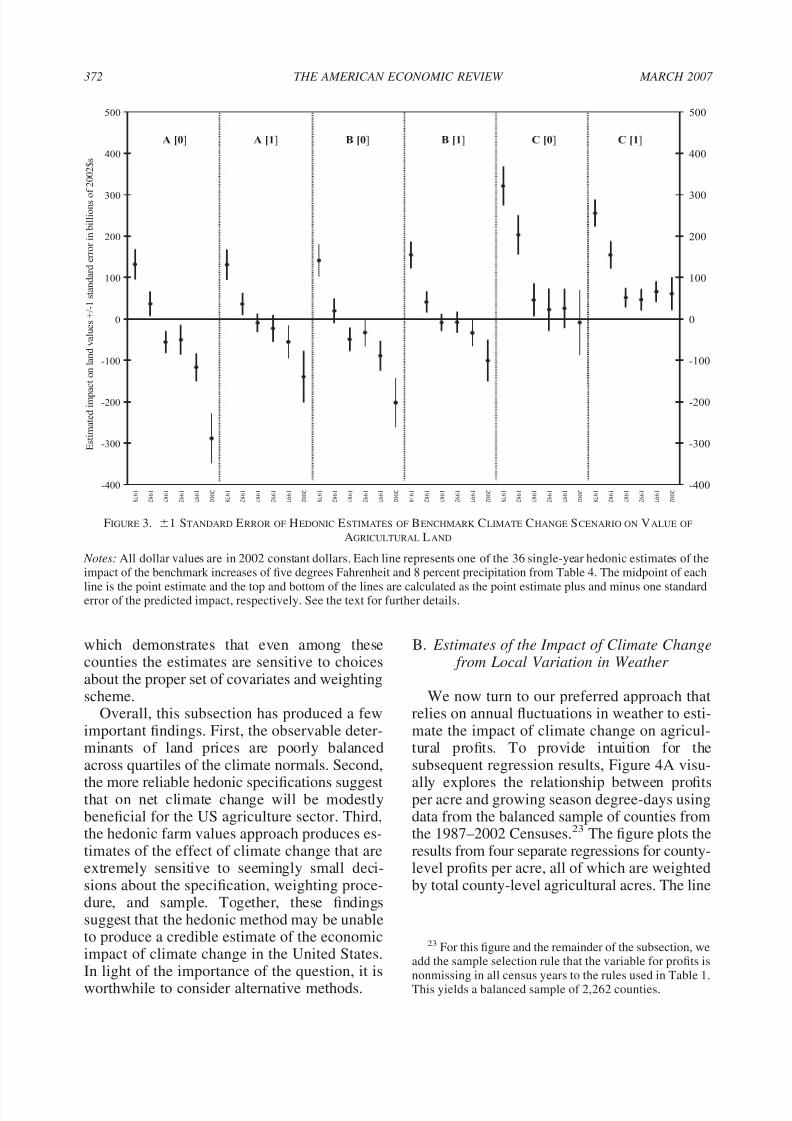
7/18/2019 The economic impact of climate change
http://slidepdf.com/reader/full/the-economic-impact-of-climate-change 19/32
which demonstrates that even among thesecounties the estimates are sensitive to choicesabout the proper set of covariates and weightingscheme.
Overall, this subsection has produced a fewimportant findings. First, the observable deter-minants of land prices are poorly balancedacross quartiles of the climate normals. Second,
the more reliable hedonic specifications suggestthat on net climate change will be modestlybeneficial for the US agriculture sector. Third,the hedonic farm values approach produces es-timates of the effect of climate change that areextremely sensitive to seemingly small deci-sions about the specification, weighting proce-dure, and sample. Together, these findingssuggest that the hedonic method may be unableto produce a credible estimate of the economicimpact of climate change in the United States.In light of the importance of the question, it isworthwhile to consider alternative methods.
B. Estimates of the Impact of Climate Change from Local Variation in Weather
We now turn to our preferred approach thatrelies on annual fluctuations in weather to esti-mate the impact of climate change on agricul-tural profits. To provide intuition for thesubsequent regression results, Figure 4A visu-
ally explores the relationship between profitsper acre and growing season degree-days usingdata from the balanced sample of counties fromthe 1987–2002 Censuses.23 The figure plots theresults from four separate regressions for county-level profits per acre, all of which are weightedby total county-level agricultural acres. The line
23 For this figure and the remainder of the subsection, weadd the sample selection rule that the variable for profits isnonmissing in all census years to the rules used in Table 1.This yields a balanced sample of 2,262 counties.
-400
-300
-200
-100
0
100
200
300
400
500
1 9 7 8
1 9 8 2
1 9 8 7
1 9 9 2
1 9 9 7
2 0 0 2
1 9 7 8
1 9 8 2
1 9 8 7
1 9 9 2
1 9 9 7
2 0 0 2
1 9 7 8
1 9 8 2
1 9 8 7
1 9 9 2
1 9 9 7
2 0 0 2
1 9 7 8
1 9 8 2
1 9 8 7
1 9 9 2
1 9 9 7
2 0 0 2
1 9 7 8
1 9 8 2
1 9 8 7
1 9 9 2
1 9 9 7
2 0 0 2
1 9 7 8
1 9 8 2
1 9 8 7
1 9 9 2
1 9 9 7
2 0 0 2
E s t i m a t e d i m p a c t o n l a n d v a l u e s + / - 1 s t a n d a r d e r r o r i n b i l l i o n s o
f 2 0 0 2 $ s
-400
-300
-200
-100
0
100
200
300
400
500
A [0] C [0]B [1]B [0]A [1] C [1]
FIGURE 3. 1 STANDARD ERROR OF HEDONIC ESTIMATES OF BENCHMARK CLIMATE CHANGE SCENARIO ON VALUE OF
AGRICULTURAL LAND
Notes: All dollar values are in 2002 constant dollars. Each line represents one of the 36 single-year hedonic estimates of theimpact of the benchmark increases of five degrees Fahrenheit and 8 percent precipitation from Table 4. The midpoint of each
line is the point estimate and the top and bottom of the lines are calculated as the point estimate plus and minus one standarderror of the predicted impact, respectively. See the text for further details.
372 THE AMERICAN ECONOMIC REVIEW MARCH 2007
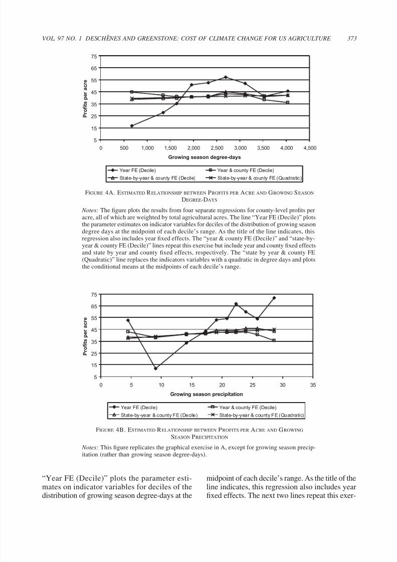
7/18/2019 The economic impact of climate change
http://slidepdf.com/reader/full/the-economic-impact-of-climate-change 20/32
“Year FE (Decile)” plots the parameter esti-mates on indicator variables for deciles of thedistribution of growing season degree-days at the
midpoint of each decile’s range. As the title of theline indicates, this regression also includes yearfixed effects. The next two lines repeat this exer-
5
15
25
35
45
55
65
75
0 5 10 15 20 25 30 35
Growing season precipitation
P r o f i t s p e r a c r e
Year FE (Decile) Year & county FE (Decile)
State-by-year & county FE (Decile) State-by-year & county FE (Quadratic)
FIGURE 4B. ESTIMATED RELATIONSHIP BETWEEN PROFITS PER ACRE AND GROWING
SEASON PRECIPITATION
Notes: This figure replicates the graphical exercise in A, except for growing season precip-itation (rather than growing season degree-days).
5
15
25
35
45
55
65
75
0 500 1,000 1,500 2,000 2,500 3,000 3,500 4,000 4,500
Growing season degree-days
P r o f i t s p
e r a c r e
Year FE (Decile) Year & county FE (Decile)
State-by-year & county FE (Decile) State-by-year & county FE (Quadratic)
FIGURE 4A. ESTIMATED RELATIONSHIP BETWEEN PROFITS PER ACRE AND GROWING SEASON
DEGREE-DAYS
Notes: The figure plots the results from four separate regressions for county-level profits peracre, all of which are weighted by total agricultural acres. The line “Year FE (Decile)” plotsthe parameter estimates on indicator variables for deciles of the distribution of growing seasondegree days at the midpoint of each decile’s range. As the title of the line indicates, thisregression also includes year fixed effects. The “year & county FE (Decile)” and “state-by-year & county FE (Decile)” lines repeat this exercise but include year and county fixed effectsand state by year and county fixed effects, respectively. The “state by year & county FE(Quadratic)” line replaces the indicators variables with a quadratic in degree days and plotsthe conditional means at the midpoints of each decile’s range.
373VOL. 97 NO. 1 DESCHE ˆ NES AND GREENSTONE: COST OF CLIMATE CHANGE FOR US AGRICULTURE

7/18/2019 The economic impact of climate change
http://slidepdf.com/reader/full/the-economic-impact-of-climate-change 21/32
cise but include year and county fixed effects andstate by year and county fixed effects, respec-tively. The final line replaces degree-day decileindicators with a quadratic in degree-days andplots the conditional means at the midpoints of
each decile’s range. It is labeled “State by Year &County FE (Quadratic).”
There are several important findings in thisgraph. First, in the “Year FE” line there istremendous variation in profits per acre. Nota-bly, it peaks in the sixth decile (midpoint 2,697 degree-days), which includes the overallmean of roughly 2,850. Second, the addition of county fixed effects to the specification greatlyreduces the variation in profits per acre. Theinclusion of state by year fixed effects further
mitigates it. This finding is consistent with thehedonic results that temperature is confoundedby many other factors, and a failure to adjust forthem will lead to severely biased estimates of itseffect. Third, the modeling of degree-days witha quadratic provides a good approximation tothe less parametric approach. Fourth, and mostimportant, the adjusted models show that evenrelatively large changes in degree-days willhave modest effects on profits per acre. Thisforeshadows the degree-day results from theestimation of equation (4).
Figure 4B repeats this exercise for precipitationand leads to similar conclusions. After adjustmentfor county fixed effects, the response surfaces arequite flat. They all suggest that the Hadley 2 pre-dicted average increase of three inches of precip-itation will have a small impact on profits per acre.
Table 5 presents estimates of the impact of three climate change scenarios on agriculturalprofits. These results are derived from the esti-mation of four versions of equation (4). Grow-ing season degree-days and precipitation are
both modeled with a quadratic and allowed todiffer in nonirrigated and irrigated counties. Theindividual parameter estimates and their stan-dard errors are presented in the Web AppendixTable 4. Each specification includes a full set of county fixed effects. In columns 1 and 2, thespecification includes unrestricted year effects,and these are replaced with state by year effectsin columns 3 and 4. Additionally, the column 2and 4 specifications adjust for the full set of soilvariables listed in Table 1, while the column 1and 3 estimating equations do not include thesevariables. All equations are weighted by the
square root of total acres of farmland. The speci-fication details are noted at the bottom of the table.
Due to the nonlinear modeling of the weathervariables, each county’s predicted impact is cal-culated as the discrete difference in per acre
profits at the county’s predicted degree-daysand precipitation after climate change and itscurrent climate (i.e., the average over the 1970–2000 period).24 The resulting change in per acreprofits is multiplied by the number of acres of farmland in the county, and then the nationaleffect is obtained by summing across all 2,262counties in the sample. The irrigated (nonirri-gated) weather parameters are used to calculatethe effect for irrigated (nonirrigated) counties.
We focus here on the Hadley 2 long-run
(2070–2099) scenario that allows for state-levelvariation in the change in degree-days and precip-itation. The preferred estimates from the column 4specification with soil controls and state by yearfixed effects suggest that climate change will leadto an increase in agricultural sector profits of roughly $1.3 billion. This estimate is statisticallyindistinguishable from zero with either the Eicker-White (parentheses) or Conley (square brackets)standard errors. With the smaller standard errors,the 95-percent confidence interval ranges fromabout $0.5 billion to $3.1 billion. In the context
of the mean annual profits of $32.3 billion over the1987–2002 period, these estimates imply that it isunlikely that climate change will have large neg-ative or positive impacts on agricultural profits.The qualitative conclusions from the other scenar-ios are identical.
A few other features of the results are note-worthy. First, after adjustment for the state byyear effects, the predicted change in precipita-tion has a statistically significant and positiveimpact on profits. Second when the point esti-
mates are taken literally, the overall effect isalmost entirely concentrated in nonirrigatedcounties.25 Third, the results from all scenariosfollow a similar pattern in that the column 1 and
24 Since the Hadley 2 predictions are at the state level,each county is assigned its state’s prediction.
25 We also estimated “fully interacted” models that al-lowed all parameters (e.g., the year or state by year fixedeffects and soil parameters) to vary across irrigated andnonirrigated counties. The estimated national impact of climate change is virtually unchanged in the column (1)–(4)specifications.
374 THE AMERICAN ECONOMIC REVIEW MARCH 2007
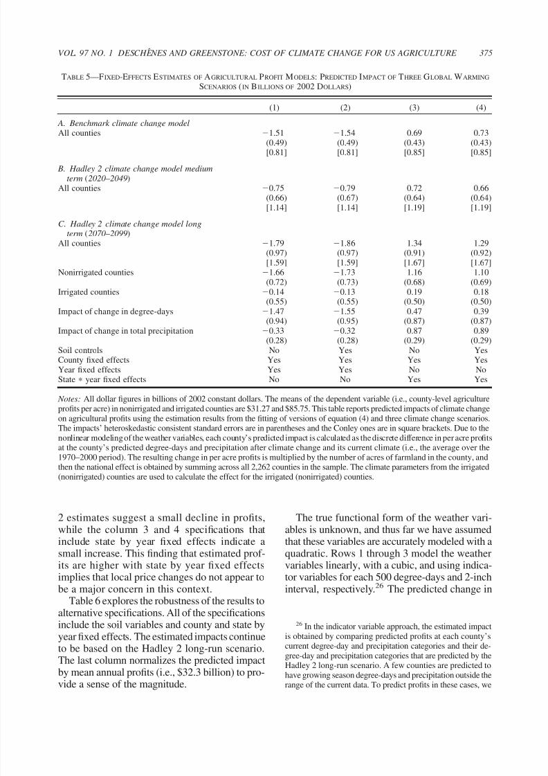
7/18/2019 The economic impact of climate change
http://slidepdf.com/reader/full/the-economic-impact-of-climate-change 22/32
2 estimates suggest a small decline in profits,while the column 3 and 4 specifications that
include state by year fixed effects indicate asmall increase. This finding that estimated prof-its are higher with state by year fixed effectsimplies that local price changes do not appear tobe a major concern in this context.
Table 6 explores the robustness of the results toalternative specifications. All of the specificationsinclude the soil variables and county and state byyear fixed effects. The estimated impacts continueto be based on the Hadley 2 long-run scenario.The last column normalizes the predicted impactby mean annual profits (i.e., $32.3 billion) to pro-vide a sense of the magnitude.
The true functional form of the weather vari-ables is unknown, and thus far we have assumed
that these variables are accurately modeled with aquadratic. Rows 1 through 3 model the weathervariables linearly, with a cubic, and using indica-tor variables for each 500 degree-days and 2-inchinterval, respectively.26 The predicted change in
26 In the indicator variable approach, the estimated impactis obtained by comparing predicted profits at each county’scurrent degree-day and precipitation categories and their de-gree-day and precipitation categories that are predicted by theHadley 2 long-run scenario. A few counties are predicted tohave growing season degree-days and precipitation outside therange of the current data. To predict profits in these cases, we
TABLE 5—FIXED-EFFECTS ESTIMATES OF AGRICULTURAL PROFIT MODELS: PREDICTED IMPACT OF THREE GLOBAL WARMING
SCENARIOS (IN BILLIONS OF 2002 DOLLARS)
(1) (2) (3) (4)
A. Benchmark climate change model
All counties 1.51 1.54 0.69 0.73(0.49) (0.49) (0.43) (0.43)[0.81] [0.81] [0.85] [0.85]
B. Hadley 2 climate change model mediumterm (2020–2049)
All counties 0.75 0.79 0.72 0.66(0.66) (0.67) (0.64) (0.64)[1.14] [1.14] [1.19] [1.19]
C. Hadley 2 climate change model longterm (2070–2099)
All counties 1.79 1.86 1.34 1.29(0.97) (0.97) (0.91) (0.92)[1.59] [1.59] [1.67] [1.67]
Nonirrigated counties 1.66 1.73 1.16 1.10(0.72) (0.73) (0.68) (0.69)
Irrigated counties 0.14 0.13 0.19 0.18(0.55) (0.55) (0.50) (0.50)
Impact of change in degree-days 1.47 1.55 0.47 0.39(0.94) (0.95) (0.87) (0.87)
Impact of change in total precipitation 0.33 0.32 0.87 0.89(0.28) (0.28) (0.29) (0.29)
Soil controls No Yes No YesCounty fixed effects Yes Yes Yes YesYear fixed effects Yes Yes No NoState year fixed effects No No Yes Yes
Notes: All dollar figures in billions of 2002 constant dollars. The means of the dependent variable (i.e., county-level agriculture
profits per acre) in nonirrigated and irrigated counties are $31.27 and $85.75. This table reports predicted impacts of climate changeon agricultural profits using the estimation results from the fitting of versions of equation (4) and three climate change scenarios.The impacts’ heteroskedastic consistent standard errors are in parentheses and the Conley ones are in square brackets. Due to thenonlinear modeling of the weather variables, each county’s predicted impact is calculated as the discrete difference in per acre profitsat the county’s predicted degree-days and precipitation after climate change and its current climate (i.e., the average over the1970–2000 period). The resulting change in per acre profits is multiplied by the number of acres of farmland in the county, andthen the national effect is obtained by summing across all 2,262 counties in the sample. The climate parameters from the irrigated(nonirrigated) counties are used to calculate the effect for the irrigated (nonirrigated) counties.
375VOL. 97 NO. 1 DESCHE ˆ NES AND GREENSTONE: COST OF CLIMATE CHANGE FOR US AGRICULTURE

7/18/2019 The economic impact of climate change
http://slidepdf.com/reader/full/the-economic-impact-of-climate-change 23/32
profits is positive in all three of these approaches,but a zero effect cannot be rejected in any of thecases.
Row 4 considers the possibility of harmful
degree-days. Harmful degree days are calcu-lated by summing each growing season day’sharmful degree-days. The traditional way to cal-culate a day’s harmful degree-days is that a daywith a mean temperature above 93.2°F contrib-utes the difference between the mean and93.2°F, while a day with a mean temperaturebelow 93.2°F contributes zero degree days.There is no empirical support in our data toestimate such effects, however, because the av-erage county in the United States faced 0.2
growing season degree-days of such harmfultemperatures during our sample. Rather thandefining harmful degree-days on the basis of mean daily temperature, we define harmful de-
gree-days using the maximum daily tempera-ture, as suggested by SHF (2006). Although thisalternative measure is not the norm in the agron-omy literature, it greatly increases the number
of harmful degree-days per growing season—from 0.2 to 30 on average per county—so itseffect can be estimated from the data.
In row 4 we follow the specification of SHF(2006) and model the impact of harmful degree-days with a square root, again allowing its effectto vary across irrigated and nonirrigated coun-ties. We also include this measure of harmfuldegree-days in our calculation of the impacts of climate change. The table reveals that the re-sulting estimate of the impact of climate change
on agricultural profits is practically unchangedby the inclusion of controls for damagingdegree-days.
Row 5 explores the possibility that outliersdrive the results in Table 5. Specifically, it pre-sents the results from the “rreg” robust regres-sion routine in STATA (Berk 1990). Thisroutine begins by excluding outliers, defined asobservations with values of Cook’s D 1, andthen weights observations based on absoluteresiduals so that large residuals are down-weighted. The entry indicates that the qualita-tive finding is unchanged.
assign the average change in profits associated with a 1-cate-gory change across the entire range of current data for each 500degree-day or 2-inch category increase. For example, if acounty is currently in the highest 500 degree-day category andmoves up two 500 degree-day categories under the Hadley 2scenario, its predicted increase in profits equals two times theaverage change in profits associated with an increase in a500-degree category over the current range of data.
TABLE 6—ALTERNATIVE FIXED-EFFECTS ESTIMATES OF HADLEY 2 LONG-RUN CLIMATE CHANGE SCENARIO ON
AGRICULTURAL PROFITS
Hadley 2 long run (2070–2099)
Predicted change
(billion dollars)
Standard
error
Percent
effect(1) Model weather variables linearly 1.47 (0.75) 4.6(2) Model weather variables with cubics 3.59 (2.03) 11.1(3) Model weather variables with indicator variables 0.75 (1.34) 2.3(4) Control for harmful degree-days 1.33 (0.93) 4.1(5) Minimize the influence of outliers 0.24 (0.41) 0.7(6) Fully interacted by state 0.17 (11.00) 0.5(7) Irrigation cutoff 5% 1.23 (0.91) 3.8(8) Irrigation cutoff 15% 1.29 (0.97) 4.0(9) Assume equal weather coefficients in nonirrigated and
irrigated counties1.27 (0.99) 3.9
(10) Growing season April–October 0.57 (2.02) 1.8(11) Two growing seasons, April–October and November–March 0.98 (5.04) 3.0(12) Unweighted regression 0.52 (2.46) 1.6
Notes: All dollar figures in billions of 2002 constant dollars. The entries report predicted impacts of climate change onagricultural profits using the estimation results from alternative versions of equation (4) and the Hadley 2 long-run climatechange scenario. All versions of equation (4) include controls for soil productivity and county and state by year fixed effects.The impacts’ heteroskedastic consistent standard errors are in parentheses. The “percent effect” column reports the predictedchange as a percent of mean annual agricultural profits in the 1987–2002 period. See Table 6, as well as the text for furtherdetails.
376 THE AMERICAN ECONOMIC REVIEW MARCH 2007

7/18/2019 The economic impact of climate change
http://slidepdf.com/reader/full/the-economic-impact-of-climate-change 24/32
Row 6 summarizes the results from estimatingseparate versions of equation (4) for each of the 48states. Thus, all the parameters are allowed to varyat the state-level. The effect of the weather vari-ables is allowed to vary across irrigated and non-
irrigated counties within each state. The sum of the state-specific estimates of the impact isroughly $0.2 billion. The heavy demands that thisapproach places on the data are evident in the poorprecision of this estimate.27
The remaining rows lead to the same quali-tative conclusion that climate change will haveonly a modest effect on agricultural profits.Rows 7 through 9 indicate that the results arelargely insensitive to how counties are assignedto the irrigated and nonirrigated categories and
whether the weather parameters are allowed tovary across these groups. In row 10 the growingseason is extended by a month to include Oc-tober, and in row 11 we allow for two growingseasons that cover the entire year to allow forthe effect of the important winter wheat crop.The predicted change remains small and statis-tically insignificant in these rows. In row 12, theregression equation is unweighted, which in-creases the estimated standard error by morethan 250 percent but leaves the qualitative find-ing unaltered.
Table 7 explores the distributional conse-quences of climate change across states. It liststhe predicted impact of the Hadley 2 long-runclimate change scenario on state-level agricul-tural profits. The states are ordered by the im-pact on profits and the percentage change inprofits from largest to smallest in columns 1 and2, respectively. The entries are based on theestimation of a separate version of equation (4)for each state. The sum of these effects is $0.2billion and was reported in row 6 of Table 6.
The most striking finding is that California willbe significantly harmed by climate change. Its lossin agricultural profits is approximately $750 mil-lion, and this is nearly 15 percent of total Califor-nia agricultural profits. To place this estimate infurther context, the remaining 47 states are pre-dicted to have a gain of $930 million. Nebraska
($670 million) and North Carolina ($650 mil-lion) are also predicted to have big losses, whilethe two biggest winners are South Dakota ($720million) and Georgia ($540 million). It would beremiss not to point out that in general these state-
specific predictions are imprecise and the null of zero can be rejected at the 5-percent level or betterfor only eight states (i.e., Montana, Nebraska,New York, North Carolina, North Dakota, SouthCarolina, South Dakota, and Pennsylvania).
Overall, the estimates in this subsection sug-gest that the predicted changes in climate willlead to economically and statistically smallchanges in profits. The preferred estimates sug-gest an increase in profits and have a 95-percentconfidence interval that ranges from a change in
profits of $0.5 billion to $3.1 billion, or 1.5percent to 9.6 percent. Thus, large negative orpositive effects are unlikely.
C. Estimates of the Response of Crop Yieldsto Climate Change
In this subsection, we explore the effect of predicted climate change on crop yields. Largedeclines in yields would suggest that the profitresults may be biased (relative to the preferredlong-run measure) by short-run price increases.
Although farmers cannot switch crops in re-sponse to weather shocks, they are able to un-dertake some adaptations, and in this respectthis approach is preferable to the productionfunction approach.
Table 8 presents the results from the estima-tion of versions of equation (4), where the de-pendent variables are county-level total bushelsof production per acre planted (production/acreplanted) for corn for grain and soybeans. Theindependent variables of interest are growing
season degree-days and precipitation, both of which are modeled with a quadratic and allowedto vary by irrigation status of the county. Theregressions all include controls for soil charac-teristics and county fixed effects and areweighted by the square root of the number of acres planted. The “a” specifications includeyear fixed effects and the “b” ones have state byyear fixed effects. The sample is drawn from the1987, 1992, 1997, and 2002 Censuses, and foreach crop it is limited to the counties withproduction of the crop in each of these years.These two crops account for roughly $39 billion
27 There are a total of 22 parameters, so this model cannotbe estimated separately for the 11 states with fewer than 22counties in our sample. Instead, we group these states togetherin two groups (AZ, NV) and (CT, DE, MA, MD, ME, NH, NJ,RI, VT) and estimate the model separately for each group.
377 VOL. 97 NO. 1 DESCHE ˆ NES AND GREENSTONE: COST OF CLIMATE CHANGE FOR US AGRICULTURE

7/18/2019 The economic impact of climate change
http://slidepdf.com/reader/full/the-economic-impact-of-climate-change 25/32
TABLE 7—FIXED-EFFECTS ESTIMATES OF HADLEY 2 LONG-RUN CLIMATE CHANGE SCENARIO ON AGRICULTURAL PROFITS,BY STATE
Predicted impact on state agricultural profits (largest to smallest)
State
(1a)
Billions of $s
(1b)
Std Error
(1c)
State
(2a)
Percent
(2b)South Dakota 0.72 (0.09) West Virginia 189.6Georgia 0.54 (0.61) Arizona 118.9Arizona 0.49 (0.81) South Dakota 109.2Nevada 0.49 (0.81) South Carolina 102.8Kansas 0.24 (0.15) Georgia 71.7New York 0.23 (0.07) Nevada 69.6South Carolina 0.23 (0.09) Wyoming 45.4Kentucky 0.21 (0.28) New York 43.4Pennsylvania 0.17 (0.06) Louisiana 43.2North Dakota 0.16 (0.07) North Dakota 40.0Louisiana 0.15 (0.42) Kentucky 27.1Missouri 0.10 (0.07) Utah 22.6Oregon 0.10 (0.32) Pennsylvania 20.0West Virginia 0.08 (0.10) Kansas 19.7Wyoming 0.07 (0.09) Oregon 18.3Minnesota 0.07 (0.07) Missouri 13.1Michigan 0.05 (0.05) Michigan 9.3Washington 0.04 (0.85) Indiana 5.9Utah 0.04 (0.19) Minnesota 5.6Indiana 0.04 (0.12) Washington 4.7New Mexico 0.01 (0.15) Virginia 3.0Virginia 0.01 (0.06) New Mexico 2.4Oklahoma 0.00 (0.15) Oklahoma 0.2Idaho 0.00 (0.10) Idaho 0.6Iowa 0.01 (0.07) Iowa 0.9Connecticut 0.03 (0.10) Wisconsin 2.5Delaware 0.03 (0.10) Tennessee 9.2Massachusetts 0.03 (0.10) Texas 10.0Maryland 0.03 (0.10) Ohio 10.2Maine 0.03 (0.10) Illinois 12.1New Hampshire 0.03 (0.10) Maryland 12.7New Jersey 0.03 (0.10) Arkansas 13.0Rhode Island 0.03 (0.10) California 15.0Vermont 0.03 (0.10) New Jersey 18.2Tennessee 0.03 (0.07) Delaware 23.2Wisconsin 0.03 (0.05) Connecticut 25.5Ohio 0.07 (0.08) Massachusetts 28.3Arkansas 0.11 (0.27) Maine 28.3Montana 0.12 (0.06) Florida 28.6Mississippi 0.16 (0.18) Colorado 36.3Texas 0.16 (0.50) Vermont 36.4Illinois 0.18 (0.13) Montana 40.2Colorado 0.21 (0.22) Nebraska 40.8Alabama 0.21 (0.33) Mississippi 42.7Florida 0.45 (0.44) North Carolina 46.0North Carolina 0.65 (0.24) Alabama 46.7Nebraska 0.67 (0.22) Rhode Island 84.9California 0.75 (1.50) New Hampshire 127.4
Notes: All figures in billions of 2002 constant dollars. The entries report state-level predicted impacts of climate change onagricultural profits using the estimation results from state-level versions of equation (4) and the Hadley 2 long-run climatechange scenario. Growing season degree-days and total precipitation are modeled with quadratics, and their effects areallowed to vary in irrigated and nonirrigated counties. The specification also includes controls for soil productivity and countyand year fixed effects. There are a total of 22 parameters, so this model cannot be estimated separately for the 11 states withfewer than 22 counties in our sample. Instead, we group these states together in two groups (AZ, NV) and (CT, DE, MA, MD,ME, NH, NJ, RI, VT) and estimate the model separately for each group. See the text for more details.
378 THE AMERICAN ECONOMIC REVIEW MARCH 2007

7/18/2019 The economic impact of climate change
http://slidepdf.com/reader/full/the-economic-impact-of-climate-change 26/32
of revenues when their output is evaluated at theaverage crop price over these years, which isabout 22 percent of total agricultural revenues.
The second panel reports the predictedchange in national output in billions of bushels
and its standard error under the Hadley 2 long-run scenario. Each county’s predicted change inbushels per acre is calculated as the discretedifference in per acre output at the county’spredicted degree-days and precipitation afterclimate change and its current climate (i.e., theaverage over the 1970–2000 period). The re-sulting change in bushels per acre is multipliedby the number of acres of farmland in thecounty, and then the national effect is obtainedby summing across all counties in the sample.The next row presents this change as a percent-age of the average yield in our balanced sample
of counties. The other rows report the change inbushels in nonirrigated and irrigated countiesand the separate impacts of the predictedchanges in temperature and precipitation.
The results are consistent across the crops.
Specifically, the more robust model with stateby year fixed effects fails to find a statisticallysignificant relationship between climate changeand crop yields for either of the crops. The lessrobust “a” specification finds negative effectsfor corn and soybeans, but they are small inmagnitude.28 In general, the increase in temper-
28 David B. Lobell and Gregory P. Asner (2003a) find anegative relationship between county level corn and soy-bean yield trends and trends in mean temperatures. Thereare a number of differences between Lobell and Asner’sapproach and this paper’s approach that make comparisons
TABLE 8—FIXED-EFFECTS ESTIMATES OF AGRICULTURAL YIELD MODELS
Corn for grain Soybeans
(1a) (1b) (2a) (2b)
US total value (billion dollars) 22.54 22.54 16.32 16.32
County mean of dep. variable 114.77 114.77 36.63 36.63US total production (billion bushels) 8.67 8.67 2.38 2.38
Predicted impact of Hadley 2 long-term(2070–2099) scenario on crop yields
All counties 0.06 0.01 0.05 0.02(0.07) (0.07) (0.02) (0.02)
Percent of US total yield 0.7 0.1 2.0 0.7Nonirrigated counties 0.10 0.00 0.04 0.01
(0.06) (0.05) (0.01) (0.01)Irrigated counties 0.04 0.01 0.01 0.00
(0.03) (0.03) (0.01) (0.01)Impact of change in temperature 0.34 0.16 0.12 0.04
(0.07) (0.06) (0.02) (0.01)
Impact of change in precipitation 0.28 0.17 0.07 0.05(0.03) (0.02) (0.01) (0.01)
Soil controls Yes Yes Yes YesCounty fixed effects Yes Yes Yes YesYear fixed effects Yes No Yes NoState year fixed effects No Yes No Yes
Notes: “US total value” is expressed in billions of 2002 constant dollars. The row “county mean of dependent variable” isexpressed in bushels per acre and “US total yield” is in billions of bushels. The other entries report predicted impacts of climate change on crop output (in billions of bushels) using the estimation results from versions of equation (4) and the Hadley 2long-run climate change scenario. In the versions of equation (4), the dependent variables are county-level total bushels of production per acre planted (production/acre planted) for corn for grain, soybeans, and wheat for grain. The independentvariables of interest are growing season degree-days and precipitation, both of which are modeled with a quadratic andallowed to vary among nonirrigated and irrigated counties. The regressions all include controls for soil characteristics and
county fixed effects and are weighted by the square root of the number of acres planted for the relevant crop. Due to thenonlinear modeling of the weather variables, each county’s predicted change in bushels per acre is calculated as the discretedifference in per acre output at the county’s predicted degree-days and precipitation after climate change and its currentclimate (i.e., the average over the 1970–2000 period). The resulting change in bushels per acre is multiplied by the numberof acres of farmland in the county and then the national effect is obtained by summing across all counties in the sample. Thereare 5,992 observations in columns 1a and 1b and 4,320 in columns 2a and 2b.
379VOL. 97 NO. 1 DESCHE ˆ NES AND GREENSTONE: COST OF CLIMATE CHANGE FOR US AGRICULTURE

7/18/2019 The economic impact of climate change
http://slidepdf.com/reader/full/the-economic-impact-of-climate-change 27/32
ature is harmful for yields and the increase inprecipitation is beneficial. This finding under-scores that it is important to account for both thechange in temperature and precipitation whenassessing the impacts of climate change. In
summary, the small changes in output or quan-tities suggest that it is unlikely that the previoussubsection’s finding that climate change willhave a small effect on agricultural profits is dueto short-run price increases.
V. Interpretation
Optimal decisions about climate change pol-icies require estimates of individuals’ willing-ness to pay to avoid climate change over the
long run. The analysis above has developedmeasures of the impact of climate change on theprofits from agricultural operations that accrueto the owners of land. Since land values ulti-mately reflect the present discounted value of land rents, or profits from land, we use theestimates from the previous section to develop ameasure of the welfare consequences of climatechange. We assume that the predicted increaseof $1.3 billion (from column 4 of Table 5 andthe long-run Hadley 2 model) in annual agricul-tural profits holds for all years in the future, and
we apply a discount rate of 5 percent. Thisimplies that climate change increases thepresent value of the stream of land rents byabout $26 billion. The 95-percent confidenceinterval is $10 billion to $62 billion. Thisrange is much tighter than the range of pointestimates from the hedonic approach, and thatrange would be even wider if it accounted forsampling variability.
There are a number of important caveats tothese calculations and, more generally, to the
analysis. First, some models of climate changepredict increases in extreme events (e.g.,droughts and floods) or the variance of climaterealizations, in addition to any effects on grow-ing season degree-days and precipitation. Our
analysis is uninformative about the economicimpact of these events. If the predictions aboutthese events are correct, a full accounting of thewelfare effects of climate change would have toadd the impacts of these changes to the impacts
presented here. Similarly, it is thought that per-manent changes in climate will disrupt localecosystems and/or change soil quality. Both of these factors may affect agricultural productiv-ity. Since annual fluctuations in climate are un-likely to have the same effect on ecosystemsand soil quality as permanent changes, our es-timates also fail to account for these effects.
Second, as its name suggests, global climatechange will affect agricultural productionaround the globe. It may be reasonable to as-
sume that this will alter the long-run costs of production, and this would cause changes inrelative prices. Since our estimates are based onannual fluctuations in weather and are adjustedfor state by year fixed effects, it is unlikely thatthey fully account for this possibility. It is note-worthy that the hedonic approach is unable toaccount for such changes either, because theland value-climate gradient is estimated overthe existing set of prices.
Third, there is a complex system of govern-ment programs that have an impact on agricul-
tural profits and land values by affectingfarmers’ decisions about which crops to plant,the amount of land to use, and the level of production (Kirwan 2005). Our estimates wouldlikely differ if they were estimated with analternative set of subsidy policies in force. Thiscaveat also applies to the hedonic method.
Fourth, our measure of agricultural profitsdiffers from an ideal one in some importantrespects. In particular, interest payments are theonly measure of the rental cost of capital in the
Censuses. Thus, our measure understates thecost of capital by not accounting for the oppor-tunity cost of the portion of the capital stock thatis not leveraged. Further, our measure of agri-cultural profits does not account for labor coststhat are not compensated with wages (e.g., thelabor provided by the farm owner).
Finally, we discuss two caveats to our ap-proach that would lead to an overstatement of the damage associated with climate change.First, as we have emphasized, our approachdoes not allow for the full set of adaptationsavailable to farmers. In this case, the direction
of the results difficult, including that Lobell and Asner: limitthe sample to counties that exhibit a negative correlationbetween temperature and yields (see Lianhong Gu 2003;Lobell and Asner 2003b); do not adjust their estimates forstate shocks (e.g., by including state fixed effects) orchanges in precipitation; and use mean temperature over thegrowing season, rather than degree-days.
380 THE AMERICAN ECONOMIC REVIEW MARCH 2007

7/18/2019 The economic impact of climate change
http://slidepdf.com/reader/full/the-economic-impact-of-climate-change 28/32
of the bias can be signed, because farmers willundertake these adaptations only if the benefitsexceed the costs.
Second, elevated carbon dioxide (CO2) con-
centrations are known to increase the yield per
planted acre for many plants (see, e.g., F. Migli-etta et al. 1998). Since higher CO
2 concentra-
tions are thought to be a primary cause of climate change, it may be reasonable to assumethat climate change will lead to higher yieldsper acre. The approach proposed in this paperdoes not account for this “fertilizing” effect of increased CO
2 concentrations.
VI. Conclusions
This study proposes and implements a newstrategy to estimate the impact of climate changeon the US agricultural sector. The strategy ex-ploits the presumably random year-to-year varia-tion in temperature and precipitation to estimatetheir effect on agricultural profits. Specifically, weuse a county-level panel data file constructed fromthe Census of Agriculture to estimate the effect of weather on agricultural profits, conditional oncounty and state by year fixed effects.
Using long-run climate change predictions
from the Hadley 2 Model, the preferred estimatesindicate that climate change will lead to a $1.3billion (2002$), or 4.0 percent, increase in annualagricultural sector profits. The 95-percent confi-dence interval ranges from $0.5 billion to $3.1billion, so large negative or positive effects areunlikely. The basic finding of an economicallyand statistically small effect is robust to a widevariety of specification checks, including adjust-ment for the rich set of available controls, model-ing temperature and precipitation flexibly,
estimating separate regression equations for eachstate, and implementing a procedure that mini-mizes the influence of outliers. Although the over-all effect is small, we showed that there isconsiderable heterogeneity in the predicted im-pacts across states. Additionally, the analysis in-dicates that the predicted increases in temperatureand precipitation will have virtually no effecton yields among the most important crops(i.e., corn for grain and soybeans), whichsuggests that the small effect on profits arenot due to short-run price increases.
Finally, we reexamine the hedonic farm value
approach that is predominant in the previous lit-erature. We find that the estimates of the effect of climate change on the value of agricultural landrange from $200 billion (2002$) to $320 billion(or 18 percent to 29 percent), which is an even
wider range than has been noted in the previousliterature. This variation in predicted impacts re-sults from seemingly minor decisions about theappropriate control variables, sample, and weight-ing. Despite its theoretical appeal, we concludethat the hedonic farm value method may be unre-liable in this setting.
There is room for much additional research inthe valuation of climate change. For example,there is an especial need for new research on theimpact of climate change on measures of human
health, particularly mortality rates. More gener-ally, future research should aim to produce esti-mates of the impact of climate change that have asound theoretical basis and are statistically robust.
DATA APPENDIX
I. COVARIATES IN LAND VALUE AND
AGRICULTURAL PROFITS REGRESSIONS
The following are the control variables used in
the land value and agricultural profits regressions.They are listed by the categories indicated in therow headings at the bottom of these tables. All of the variables are measured at the county level.
A. Dependent Variables: 1. Value of Landand Buildings per Acre; 2. Agricultural Profitsper Acre; 3. Bushels per Acre of Corn for Grain;and 4. Bushels per Acre of Soybeans.
B. Soil Variables: 1. K-Factor of Top Soil; 2.Slope Length; 3. Fraction Flood-Prone; 4. Frac-tion Sand; 5. Fraction Clay; 6. Fraction Irri-
gated; 7. Permeability; 8. Moisture Capacity; 9.Wetlands; and 10. Salinity.C. Socioeconomic Variables: 1. Income per
Capita; 2. Income per Capita squared; 3. Popu-lation Density; and 4. Population DensitySquared.
II. DETAILS ON DATA SOURCES
A. Census of Agriculture
The data on number of farms, land in farms,cropland, agricultural profits, and other agriculture
381VOL. 97 NO. 1 DESCHE ˆ NES AND GREENSTONE: COST OF CLIMATE CHANGE FOR US AGRICULTURE
7/18/2019 The economic impact of climate change
http://slidepdf.com/reader/full/the-economic-impact-of-climate-change 29/32
related variables are from the 1987, 1992, 1997,and 2002 Census of Agriculture. The Census of Agriculture has been conducted every five yearsstarting in 1925 and includes as a farm “everyplace from which $1,000 or more of agricultural
products were produced and sold or normallywould have been sold during the census year.”Participation in the Census of Agriculture is man-dated by law: all farmers and ranchers who re-ceive a census report form must respond even if they did not operate a farm or ranch in the censusyear. For confidentiality reasons, the public-usefiles provide only county averages or totals.
The following are definitions for some spe-cific variables that we used in the analysis:
Farm Revenues.—Farm revenues are thegross market value of all agricultural productssold before taxes and expenses in the censusyear, including livestock, poultry, and theirproducts; and crops, including nursery andgreenhouse crops and hay. All sales occurringduring the census year are included, even if thepayment has not been received.
Production Expenditures.—Production ex-penses are limited to those incurred in the op-eration of the farm business. Property taxes paid
by landlords are excluded. Also excluded areexpenditures for nonfarm activities and farm-related activities such as producing and har-vesting forest products, providing recreationalservices, and household expenses. Among theincluded items are: agricultural chemicals, com-mercial fertilizer, machine hire, rental of ma-chinery and equipment, feed for livestock andpoultry, hired farm and ranch labor, interestpaid on debts, livestock and poultry purchased,repairs and maintenance, and seed cost. All
costs incurred during the census year are in-cluded, regardless of whether the payment hasbeen made.
Land in Farms.—The acreage designated as“land in farms” consists primarily of agricul-tural land used for crops, pasture, or grazing.
Value of Land and Buildings.—Respondentswere asked to report their estimate of the currentmarket value of land and buildings owned,rented, or leased from others, and rented orleased to others. Market value refers to the
value the land and buildings would sell forunder current market conditions.
B. National Resource Inventory
County-level data on soils are taken from theNational Resource Inventory (NRI) (http:// www.nrcs.usda.gov/technical/NRI/). The NRIis a statistically based sample of land use andnatural resource conditions and trends on USnonfederal lands. The data have been collectedin approximately 800,000 points during theCensus of Agriculture years, starting in 1982.For example, information on soil permeability,salinity, soil contents (sand and clay), slopelength, K-factor, and fraction of the county ir-
rigated is available.
C. Hadley 2 State-Level and RegionalPredictions on Growing Season Degree-Days
and Precipitation
We downloaded the raw climate data fromthe Vegetation/Ecosystem Modeling and Anal-ysis Project (VEMAP) Transient Climate data-base. VEMAP was established as a project tolearn more about ecosystem dynamics throughmodels and simulations and involved a large
number of American and foreign scientists froma variety of different organizations (T. G. F.Kittel et al. 1995; Kittel et al. 1997; Kittel et al.2000). Phase 2 of VEMAP focused on transientdynamics, and the resulting database containsseveral climate change scenarios for the conti-nental United States, including the predictionsmade by the Hadley 2 Model. The climatevariables included in this dataset are dailyprecipitation and daily minimum and maxi-mum temperature. The data are given from Jan-
uary 1994 to December 2099.VEMAP measures climate data at a set of regular grid points spanning the contiguousUnited States and separated vertically and hor-izontally by 0.5 degrees. Data covering the en-tire grid were downloaded from the VEMAP2Web site. The data portal is available at http:// www.cgd.ucar.edu/vemap/dodsUSday_ds.html.
To obtain predicted impacts on temperatureand precipitation, we assume a 1-percent peryear compounded increase in both carbon di-oxide and IS92A sulphate aerosols, whichimplies that greenhouse gas concentrations
382 THE AMERICAN ECONOMIC REVIEW MARCH 2007
7/18/2019 The economic impact of climate change
http://slidepdf.com/reader/full/the-economic-impact-of-climate-change 30/32
will increase to roughly 2.5 times their cur-rent levels by the end of the twenty-first cen-tury. These assumptions about emissions andresulting climate change predictions are stan-dard assumptions and result in middle-of-the-
range predictions.We then used GIS software to place each of
these gridpoints into US states. With theseplacements, we were able to create the Hadley2 state-level predictions for each day from2020 to 2099. These state-level year by daypredictions are calculated as the simple aver-age across all grid points that fall within eachstate. From these daily predictions, we calcu-late growing season degree-days and totalprecipitation using the formulas described in
the text. These state-level Hadley 2 predic-tions are used to infer the economic costs of climate change throughout this paper. We fo-cus on the “medium-term” and “long-run”effects on climate, which are defined as thetemperature and precipitation averages acrossthe 2020–2049 and 2070–2099 predictions,respectively. The Hadley 2 Model is not pre-cise enough to use at smaller units of aggre-gation than the state.
D. Growing Season Degree-Days
We construct our measure of growing sea-son degree-days using daily data drawn fromthe National Climatic Data Center (NCDC)Summary of the Day Data (TD-3200). Thedata are daily measurements from weatherstations in the United States. In any givenyear in our sample period, there were approx-imately 8,000 stations in operation. The keyvariables used to construct degree-days arethe daily maximum and minimum tempera-
ture from each station. Using the daily mini-mum and maximum temperatures, we definethe mean daily temperature as the simple av-erage of the minimum and maximum temper-ature for a station. We then construct themean daily temperature for a county by takingthe simple average of the mean temperatureacross all stations within a county. For coun-ties without a station, we impute the averagemean temperature from the contiguous coun-ties. The degree-days variable is calculated onthe daily mean temperature for each county,as explained in Section II.
REFERENCES
Adams, Richard M. 1989. “Global ClimateChange and Agriculture: An Economic Per-spective.” American Journal of Agricultural
Economics, 71(5):1272–79.Altonji, Joseph G., Todd E. Elder, and Christo-
pher R. Taber. 2000. “Selection on Observedand Unobserved Variables: Assessing the Ef-fectiveness of Catholic School.” National Bu-reau of Economic Research Working Paper7831.
Berk, Richard A. 1990. “A Primer on RobustRegression.” In Modern Methods of Data
Analysis, ed. John Fox and J. Scott Long,292–324. Newbury Park, London, and New
Delhi: Sage Publications.Black, Dan A., and Thomas J. Kniesner. 2003.“On the Measurement of Job Risk in HedonicWage Models.” Journal of Risk and Uncer-tainty, 27(3): 205–20.
Black, Sandra E. 1999. “Do Better Schools Mat-ter? Parental Valuation of Elementary Edu-cation.” Quarterly Journal of Economics,114(2): 577–99.
Chay, Kenneth Y., and Michael Greenstone.2005. “Does Air Quality Matter? Evidencefrom the Housing Market.” Journal of Polit-
ical Economy, 113(2): 376–424.Cline, William R. 1996. “The Impact of Global
Warming on Agriculture: Comment.” Amer-ican Economic Review, 86(5): 1309–11.
Conley, T. G. 1999. “GMM Estimation withCross Sectional Dependence.” Journal of
Econometrics, 92(1): 1–45.Ekeland, Ivar, James J. Heckman, and Lars
Nesheim. 2004. “Identification and Estima-tion of Hedonic Models.” Journal of Political
Economy, 112(1): S60–109.
Greenstone, Michael, and Justin Gallagher. 2005.“Does Hazardous Waste Matter? Evidencefrom the Housing Market and the SuperfundProgram.” Massachusetts Institute of Tech-nology Department of Economics WorkingPaper 05–27.
Grierson, William. 2002.“Role of Temperaturein the Physiology of Crop Plants: Pre- andPost-Harvest.” In Handbook of Plant and Crop Physiology, ed. Mohammad Pessarakli,13–34. New York: Marcel Dekker.
Gu, Lianhong. 2003. “Comment on ’Climateand Management Contributions to Recent
383VOL. 97 NO. 1 DESCHE ˆ NES AND GREENSTONE: COST OF CLIMATE CHANGE FOR US AGRICULTURE

7/18/2019 The economic impact of climate change
http://slidepdf.com/reader/full/the-economic-impact-of-climate-change 31/32
Trends in U.S. Agricultural Yields’.” Sci-ence, 300(5625): 1505b.
Hoch, Irving. 1958. “Simultaneous EquationsBias in the Context of the Cobb-DouglasProduction Function.” Econometrica, 26(4):
566–78.Hoch, Irving. 1962. “Estimation of Production
Function Parameters Combining Time Seriesand Cross-Section Data.” Econometrica,30(1): 34–53.
Hodges, Thomas. 1991. Predicting Crop Phenol-ogy. Boca Raton: CRC Press.
Houghton, John T., G. J. Jenkins, and J. J.
Ephraums. ed. 1990. Climate Change: The IPCC Scientific Assessment . Cambridge,New York, and Melbourne: Cambridge Uni-
versity Press.Houghton, John T., L. G. Meiro Filho, B. A. Callan-
dar, N. Harris, A. Kattenburg, and K. Maskell.
ed. 1996. Climate Change 1995: The Science of Climate Change. Cambridge, New York, andMelbourne: Cambridge University Press.
Johns, T. C., R. E. Carnell, J. F. Crossley, J. M.
Gregory, J. F. B. Mitchell, C. A. Senior, S. F. B.
Tett, and R. A. Wood. 1997. “The SecondHadley Centre Coupled Ocean-AtmosphereGCM: Model Description, Spinup and Vali-dation.” Climate Dynamics, 13(2): 103–134.
Kelly, David L., Charles D. Kolstad, and Glenn T.
Mitchell. 2005. “Adjustment Costs from En-vironmental Change.” Journal of Environ-mental Economics and Management , 50(3):468–95.
Kirwan, Barrett E. 2005. “The Incidence of U.S.Agriculture Subsidies on Farmland RentalRates.” Unpublished.
Kittel, T. G. F., N. A. Rosenbloom, T. H. Painter,
and D. S. Schimel. 1995. “The VEMAP Inte-grated Database for Modeling United States
Ecosystem/Vegetation Sensitivity to ClimateChange.” Journal of Biogeography, 22(4 –5):857–862.
Kittel, T. G. F., N. A. Rosenbloom, C. Kaufman,
J. A. Royle, C. Daly, H. H. Fisher, W. P. Gib-
son, S. Aulenbach, R. McKeown, and D. S.
Schimel and VEMAP2 Participants. 2000.“VEMAP Phase 2 Historical and Future Sce-nario Climate Database,” available at http:// www.cgd.ucar.edu/vemap from the VEMAPData Group, National Center for AtmosphericResearch, Boulder, CO.
Lobell, David B., and Gregory P. Asner. 2003a.
“Climate and Management Contributions toRecent Trends in U.S. Agricultural Yields.”Science, 299(5609):1032.
Lobell, David B., and Gregory P. Asner. 2003b.
“Response to Comment on ‘Climate and
Management Contributions to RecentTrends in U.S. Agricultural Yields’.” Science,300(5625):1505c.
Mendelsohn, Robert, William D. Nordhaus, and
Daigee Shaw. 1994. “The Impact of GlobalWarming on Agriculture: A Ricardian Anal-ysis.” American Economic Review, 84(4):753–71.
Mendelsohn, Robert, William D. Nordhaus, and
Daigee Shaw. 1999. “The Impact of ClimateVariation on U.S. Agriculture.” In The Im-
pact of Climate Change on the United States Economy, ed. Robert Mendelsohnand James E. Neumann, 55–74. Cambridge,New York, and Melbourne: CambridgeUniversity Press.
Miglietta, F., V. Magliulo, M. Bindi, L. Cerio, F.P.
Vaccari, V. Loduca, and A. Peressotti. 1998.“Free Air CO
2 Enrichment of Potato (Sola-
num tuberosum L.): Development, Growthand Yield.” Global Change Biology, 4(2):163–172.
Mundlak, Yair. 1961. “Empirical Production
Function Free of Management Bias.” Journalof Farm Economics, 43(1): 44–56.
Mundlak, Yair. 2001. “Production and Supply.”In Handbook of Agricultural EconomicsVolume 1A: Agricultural Production, ed.B. L. Gardner and G. C. Rausser, 3–85.Amsterdam, London, and New York: ElsevierScience.
National Academy of Sciences, Committee on
Science Engineering and Public Policy. 1991.Policy Implications of Greenhouse Warm-
ing. Washington, DC: National AcademyPress.Plantinga, Andrew, Ruben Lubowski, and Robert
Stavins. 2002. “The Effects of Potential LandDevelopment on Agricultural Land Prices.”Harvard University Faculty Working PaperRWP02–012.
Richie, J. T., and D. S. NeSmith. 1991. “Temper-ature and Crop Development.” In ModelingPlant and Soil Systems, ed. John Hanks andJ. T. Ritchie, 5–29. Madison: American So-ciety of Agronomy.
Schlenker, Wolfram, W. Michael Hanemann, and
384 THE AMERICAN ECONOMIC REVIEW MARCH 2007

7/18/2019 The economic impact of climate change
http://slidepdf.com/reader/full/the-economic-impact-of-climate-change 32/32
Anthony C. Fisher. 2005. “Will U.S. Agricul-ture Really Benefit from Global Warming?Accounting for Irrigation in the Hedonic Ap-proach.” American Economic Review, 95(1):395–406.
Schlenker, Wolfram, W. Michael Hanemann, andAnthony C. Fisher. 2006. “The Impact of Global Warming on U.S. Agriculture: AnEconometric Analysis of Optimal GrowingConditions.” Review of Economics and Sta-tistics, 88(1): 113–25.
Thom, H.C.S. 1966. “Normal Degree-days
Above Any Base by the Universal TruncationCoefficient.” Monthly Weather Review,94(7): 461–65.
United States Department of Agriculture,
NASS. 1997. “Usual Planting and Harvest-
ing Dates for U.S. Field Crops.” Agricul-tural Handbook Number 628, available athttp://www.usda.gov/nass/pubs/uph97.htm.
White, Halbert. 1980. “A Heteroskedasticity-Consistent Covariance Matrix Estimator anda Direct Test for Heteroskedasticity.” Econo-metrica, 48(4): 817–38.
385VOL. 97 NO. 1 DESCHE ˆ NES AND GREENSTONE: COST OF CLIMATE CHANGE FOR US AGRICULTURE