1

The Economic Impact and Value The Economic Impact and Value of Aviation Infrastructureof Aviation Infrastructure

Mark HansenAviation Economics Short Course

Oct 14, 2004

2

MotivationMotivation

�Continuing pressure to justify investments in R&D and public aviation capital

�Peripheral involvement in some of these episodes

�What do we really know?

3

QuestionsQuestions

�What is the value of our aviation infrastructure?

�Do current studies correctly represent that value?

�What does the aviation infrastructure do that’s worth doing?

4

OutlineOutline

�Economic Impact Studies�Aviation Infrastructure and

Economic Growth�Economic Benefits of Aviation

Infrastructure Investment

5

Economic Impact StudiesEconomic Impact Studies

�Recent examples�Thought experiments�Conclusions

6

AviationAviation’’s Economic Impacts Economic Impact

TOTAL IMPACTS 11.6M Jobs

$1.1 Trillion (~ 10% of GDP)

Earnings $316.6B

From DirectFrom IndirectSubtotal

$337.6386.3

$723.9

$Billions

SECONDARY IMPACTS

DIRECT INDIRECT

Airline Ops.Airport Ops.General AviationAircraft Mfg.Subtotal

$106.415.810.938.6

$172.7

$Billions

$204.53.06.31.5

$215.3

Airline Pass.Gen. Aviat Pass.Travel AgentsOther Gen. Aviat.Subtotal

$Billions

Wilbur Smith Associates, April 2003

PRIMARY IMPACTS

7

PricePrice--rise scenario: GDPrise scenario: GDPAviation Contribution to GDP

1,000

750

500

250

01970 1980 1990 2000 2010 2020

Time (Year)

Aviation contribution to GDP,unrestricted demand

Aviation contribution to GDP,capacity-constrained demand

8

Aviation Economic Impact Aviation Economic Impact (Wilbur Smith Version)(Wilbur Smith Version)

� Primary Direct Impacts: Activity of firms providing aviation services, such as airlines, FBO’s, aircraft manufacturers, flight schools, ATC, etc.

� Primary Indirect Impacts: Activity of firms serving aviation visitors

� Secondary Impacts�Intermediate: Activity of suppliers to firms

providing aviation services or serving aviation visitors

�Activity generated by households who derive income from the primary and secondary impacts

9

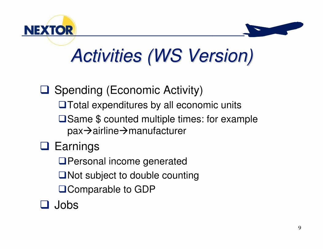
Activities (WS Version)Activities (WS Version)

� Spending (Economic Activity)�Total expenditures by all economic units�Same $ counted multiple times: for example

pax�airline�manufacturer

� Earnings�Personal income generated�Not subject to double counting�Comparable to GDP

� Jobs

10

Aviation Economic Impact (DRIAviation Economic Impact (DRI--McGraw Hill Version)McGraw Hill Version)

11

Economic MultipliersEconomic Multipliers

12

GDP Impacts of Aviation Final GDP Impacts of Aviation Final Demand: A Thought ExperimentDemand: A Thought Experiment� A family spends $2500 on a trip to

Disney world.� That $2500 includes

�$1000 for the air fare�$1500 for hotel, restaurants, rental car,

park admission, etc.

13

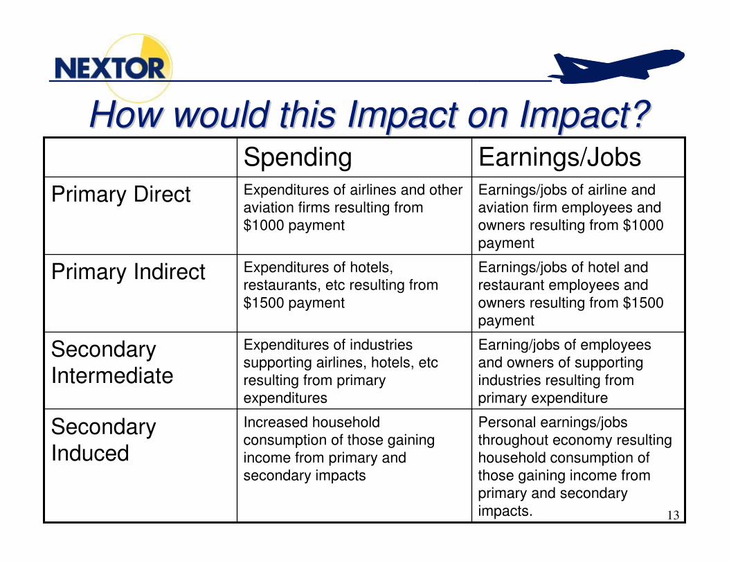
How would this Impact on Impact?How would this Impact on Impact?

Personal earnings/jobs throughout economy resulting household consumption of those gaining income from primary and secondary impacts.

Increased household consumption of those gaining income from primary and secondary impacts

Secondary Induced

Earning/jobs of employees and owners of supporting industries resulting from primary expenditure

Expenditures of industries supporting airlines, hotels, etc resulting from primary expenditures

Secondary Intermediate

Earnings/jobs of hotel and restaurant employees and owners resulting from $1500 payment

Expenditures of hotels, restaurants, etc resulting from $1500 payment

Primary Indirect

Earnings/jobs of airline and aviation firm employees and owners resulting from $1000 payment

Expenditures of airlines and other aviation firms resulting from $1000 payment

Primary Direct

Earnings/JobsSpending

14

What is the Counterfactual?What is the Counterfactual?

� To define impact we must compare two alternative scenarios

� What is the alternative scenario in the previous example?�The household does not make the trip�The money spent on the trip is hidden

under the mattress

15

More Realistic CounterfactualsMore Realistic Counterfactuals

� Some of the $2500 is spent on other consumption (also generates spending, earnings, and jobs)

� Some of the $2500 is invested (also generates spending, earnings, and jobs)

� Lacking the need for the $2500, the household works less (thus generating less spending, earnings, and jobs)

� Some of the time spent for the trip is used to work (thus generating more spending, earnings, and jobs)

16

GDP Implications of GDP Implications of Counterfactual ScenarioCounterfactual Scenario

� GDP=Consumption+Investment+Gvt.Expenditures+Exports-Imports

� Under unchanged earnings scenario� Consumption+Investment unchanged� Imports may increase or decrease� Induced consumption will increase or decrease

� Under changed earnings scenarios� Consumption+Investment may either increase or decrease� Imports may increase or decrease� Induced consumption will increase or decrease

17

ConclusionConclusion

The family trip to Disneyland has no clear implication for aggregate economic activity in terms of spending, earnings, jobs, or GDP.

18

Business TripsBusiness Trips

� GDP includes sum of value added of production units in the economy

� If a $2500 business trip occurs� Total direct and indirect value-added of firms providing

travel and their suppliers will increase $2500� Purchases of intermediate goods by traveler’s firm will

increase at least $2500, reducing the value-added of the firm by $2500

� If trip is successful, $2500 purchase will be more than counteracted by benefits (such as increased sales) resulting in net increase in value-added

� But value-added of competing firms may decrease

19

ConclusionConclusion

The family trip to Disneyland has no clear implication for aggregate economic activity in terms of spending, earnings, jobs, or GDP.

20

OutlineOutline

�Economic Impact Studies�Aviation Infrastructure and

Economic Growth�Economic Benefits of Aviation

Infrastructure Investment

21

Growth TheoryGrowth Theory� Why does the GDP grow?� Classic formulation:

� Actual GDP depends upon� Productive capacity (Potential GDP)� Demand

� If demand < potential GDP� Recession� Labor and capital underutilized� Fiscal policies to encourage growth in demand

� If demand > potential GDP� Demand temporarily satisfied by “overproduction”� Inflation

� Fiscal policies focus on keeping demand close to potential GDP in short run

� Productivity growth and increases in available inputs allow potential GDP to increase in long run

22

Aviation Economic Impact Aviation Economic Impact Studies RevisitedStudies Revisited

� Impact studies focus on the demand side of GDP

� If impacts were real, they have little policy significance�Impacts of policies would be long term�Demand-side issues are short term

� The real question is: how do aviation infrastructure investments affect productive capacity of the economy?

23

Aviation and the Growth of Aviation and the Growth of Potential GDP: Two PerspectivesPotential GDP: Two Perspectives

�Aviation as an input to production

�Aviation as a stimulus to innovation

24

Aviation as an Input to Aviation as an Input to ProductionProduction

� Aviation Infrastructure as social overhead (public) capital

� Studies examine relationship between GDP (output) and inputs including�Labor�Private capital�Public capital

25

Aviation Infrastructure as Aviation Infrastructure as Production Input Production Input

“The ultimate aim as a means of communication must be to reduce not the costs of transport, but the cost of production.” Jules Dupuit, “On the Measurement of Utility in Public Works,” 1844

26

GDP Production FunctionGDP Production Function

γβα LKAKLKKFAY GPGP =⋅= ),,(

Where:Y is GDPKP is private capitalKG is public capitalL is labor

27

AschauerAschauer AnalysisAnalysis

� Time series analysis of post-War US data� Effect of public capital found to be very

strong� $1 of public capital yields $.60 of increased

GDP� Implied underinvestment in public

infrastructure� Spawned much controversy and subsequent

analysis� See FHWA web site for summary

28

IssuesIssues

� Are statistical results realistic?� What is the direction of causality?� Public investment as a stimulus for private

investment.� Heterogeneity of public capital

�Different infrastructures�Good investments and bad investments�No studies specifically look at aviation

infrastructure

29

AviationAviation--Focused Production Function Focused Production Function Study (Gillen and Hansen, 1994)Study (Gillen and Hansen, 1994)

� Used aviation activity variables (passengers and freight enplaned) in state-level production functions

� Found that, all else equal, states with more aviation activity have higher output

� Freight effect is stronger and more statistically significant than passenger effect

30

Aviation as an Impetus to Aviation as an Impetus to Investment (Hansen, 1991)Investment (Hansen, 1991)

� Examined relationship between foreign direct investment in the United States and the initiation of international air service

� Found evidence that foreign direct investment increases after initiation of air service to the investor country

31

Aviation as a Stimulus to Aviation as a Stimulus to InnovationInnovation

� Initial impact of improvements is to do old things better

� Ultimate value rests on combining improved transport with other things�Do old things in new ways�Do new things

� These “companion innovations” by users of transportation systems drive growth and economic benefit

32

ExamplesExamples

� Bi-coastal households and extended families

� Theme parks with nation/international market areas

� One-day meeting� International corporations� Organ donor networks

33

Technological Life CycleTechnological Life Cycle

� System goes through processes of birth, growth, and maturity

� Predominant technology and initial uses of system established during birth phase

� Growth phase features rapid increases in traffic and scaling up of system, accompanied by continued discovery of new uses

� Maturity phase features slowing traffic growth� Uses fully explored and diffused throughout society (stable

demand curve)� Scale and structure makes meaningful innovation and

performance improvement difficult (stable supply curve)

34

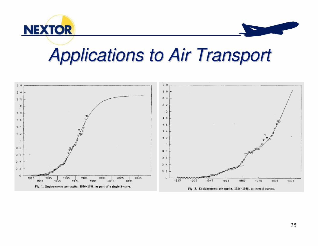
Logistic Curve (SLogistic Curve (S--Curve) Curve) (see (see GrublerGrubler, , The Rise and Fall of Infrastructures)The Rise and Fall of Infrastructures)

� Relates life-cycle to long term evolution of traffic and other system status variables

� Growth in traffic proportional to product of existing traffic and potential additional traffic:

� Solution is Lotka equation:� Interpretation

� K is saturation traffic level� t0 is time when traffic reaches half of K

)( XKXKdt

dX −= α

))(exp(1 0ttK

X−−+

=α

35

Applications to Air TransportApplications to Air Transport

36

OutlineOutline

�Economic Impact Studies�Aviation Infrastructure and

Economic Growth�Economic Benefits of Aviation

Infrastructure Investment

37

WillingnessWillingness--toto--PayPay

� Fundamental concept in assessing benefits� Net benefit of an infrastructure investment is

(arguably) positive if:

� In this case can find way to distribute benefits so that everyone is better off

� Premise for benefit-cost analysis

� >everyone

WTP 0

38

Issues with CBA/WTPIssues with CBA/WTP

� Some WTP’s may be negative� WTP not equal to what is paid� Thus projects with net benefit can be

costly or harmful to some� Best viewed as a “constitutional

principle” that everyone accepts knowing that, over many projects, they will come out ahead

39

WTP, Utility, and DemandWTP, Utility, and Demand

� Consumers and firms acquire goods and services, mostly through purchase

� Derive benefit, welfare, utility … from these goods and services

� Have preferences among different “bundles” of goods and services

40

Trends in Personal ConsumptionTrends in Personal Consumption

41

The 2The 2--Good CaseGood Case

� Assume 2 goods�One specific good that is of interest (air

transport)�One composite good that stands for all

others�Utility function becomes

),( 21 XXUU =

42

Indifference CurvesIndifference Curves

X1

X2

Bundle A

Bundle B

BA ~

43

NonNon--Satiation: More is Preferred to LessSatiation: More is Preferred to Less

X1

X2

B

E

C

D

F

G

BGFEDC �,,,,A

AGFEDC �,,,,

44

Indifference Curve MapIndifference Curve Map

X1

X2

A

B

BA ~

C

D

E

F

DC ~FE ~BC �

CF �

.

.

.

45

Perfect Substitutes and ComplementsPerfect Substitutes and Complements

X1

X2

X1

X2

46

Budget LinesBudget Lines

X1

X2

BXPXP =+ 2211

12 PP−

47

Utility MaximizationUtility MaximizationX1

X2

-P2/P1

� Maximize utility subject to a budget constraint

� Interior solution is point of tangency between budget line and indifference curve

� Corner solution if there is no such point for X1,X2>0

� Solution is unique if indifference curves are convex

X2*

X1*

48

Income EffectIncome Effect----The Engel The Engel CurveCurve

X1

X2

.

.

.

49

Normal and Inferior GoodsNormal and Inferior Goods

� Normal Good--As income (budget) increases, utility maximizing amount increases

� Inferior Good--As income (budget) increases, utility maximizing amount decreases

� Luxury Good—Consumes larger share of budget as income increases

50

Price EffectsPrice EffectsX1

-P2/P1

-P’2/P1

-P’’2/P1

X2* X2*’ X2*’’X2

Y/P1

51

Demand CurveDemand CurveP2

P2’

P2’’

X2* X2*’ X2*’’

Demand curve for good 2 given P1 nominal income Y

52

Compensated Demand CurveCompensated Demand CurveX1

-P2/P1

-P’2/P1

-P’’2/P1X2* X2*’ X2*’’X2

Utility level U

53

Compensated Demand CurveCompensated Demand CurveP2

P2’

P2’’

X2* X2*’ X2*’’

Demand curve for good 2 given P1 and utility level U.

54

Welfare MeasuresWelfare Measures----Equivalent VariationEquivalent VariationX1

X2

Y’/P1

Y/P1

),,(),,'(' 2121 PPUEPPUEYYEV −=−=

U

U’P2/P1

P2’/P1

Income required to yield the same utility gain as a price reduction.

55

Welfare MeasuresWelfare Measures----Compensating VariationCompensating VariationX1

X2

Y’/P1

Y/P1

)',,(),,(' 2121 PPUEPPUEYYCV −=−=

U

U’P2/P1

P2’/P1

Income that could be sacrificed leaving utility same as before price reduction.

56

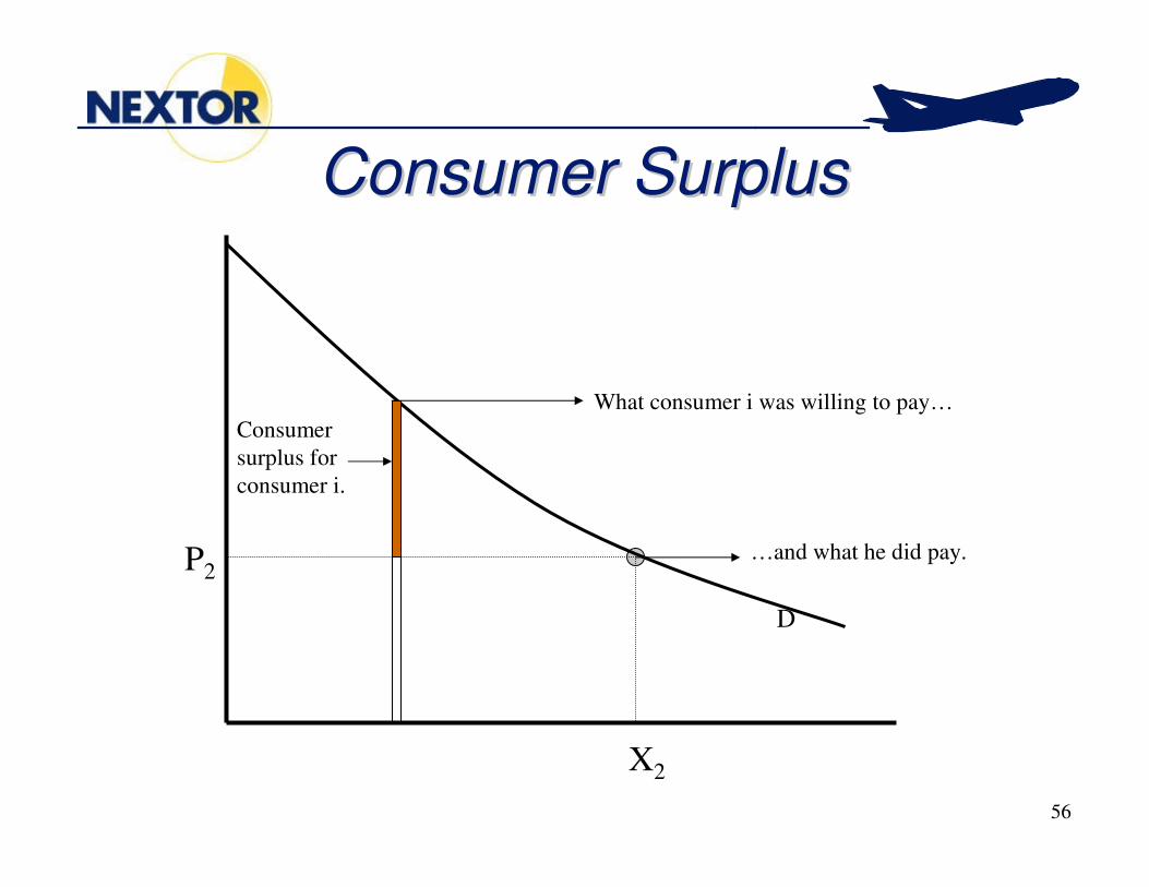
Consumer SurplusConsumer Surplus

P2

X2

What consumer i was willing to pay…

D

…and what he did pay.

Consumer surplus for consumer i.

57

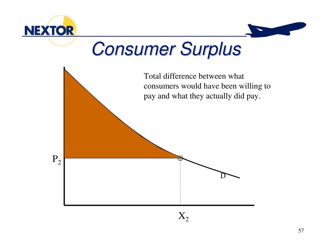
Consumer SurplusConsumer Surplus

P2

X2

D

Total difference between what consumers would have been willing to pay and what they actually did pay.

58

Change in Consumer Surplus Change in Consumer Surplus from a Price Changefrom a Price Change

P2

P2’

X2* X2*’

))(())((

)(

)()(

*22

0

*'22

0

'22

*22

02

*2

*'2

*2

XPdxxPXPdxxP

PPCS

XPdxxPPCS

XX

X

−−−

=→∆

−=

��

�

59

Rule of 1/2Rule of 1/2

� If price changes are moderate, then demand curve can be approximated as straight line between old price and new price.

� Then 2/)')('()'( XXPPPPCS +−=→∆

P

P’

X X’

60

CS,EV, and CVCS,EV, and CV

� Equivalent variation is CS using compensated demand curve at higher utility level

� Compensating variation is CS using compensated demand curve at lower utility level

� CS based on uncompensated demand curve is between EV and CV

61

Implicit Price ChangesImplicit Price Changes

� Change in service level can shift demand curve up or down

� Estimate price change that would produce the same shift

� Estimate benefits from change in service level as equivalent to from this price change

62

Implicit Price ChangeImplicit Price Change

P

P’

X X’D

D’

Shift in demand from D to D’ as a result of service improvement has same benefit as reduction in price from P to P’ on original demand curve.

63

Air Travel Demand Price Air Travel Demand Price ElasticitiesElasticities

� Sensitivity of demand curve to price� Dimensionless and thus insensitive to units

in which price and demand are measured� Assume “all else equal” including incomes,

service quality, and other prices� Two types

�Arc Elasticities�Point Elasticities

qp

PQ

arc ⋅∆∆=η

qp

PQ

point ⋅∂∂=η

64

Summary of Elasticity EstimatesSummary of Elasticity Estimates

2.170.841.39132Income

-0.50-1.46-1.02156Time Series

-0.81-1.52-1.3385Cross-section

-0.88-1.74-1.5219Short-haul Leis.

-0.61-0.80-0.7318Short-haul Bus.

-1.09-2.03-1.269Long-haul Dom. Leis.

-0.84-1.43-1.1526Long-haul Dom. Bus.

-0.54-1.65-0.9955Long-haul Inter. Leis.

-0.20-0.48-0.2616Long-haul Inter. Bus.

-0.85-1.55-1.3441Long-haul Dom.

-0.35-1.40-0.7969Long-haul Inter.

-0.73-1.54-1.15124Short/Med. Haul

-0.50-1.43-0.95105Long-haul

-0.68-1.52-1.15274All

Third Quart.First Quart.MedianNumberCategory

65

Application: Benefits of Application: Benefits of HubbingHubbingto Hub Regionsto Hub Regions

� Hansen (1998) estimates that local traffic has as an elasticity of 0.3 with respect to the hub traffic multiplier (total traffic/local traffic)

� Suppose hub region has originating traffic of 4 million and total traffic of 10 million (multiplier is 2.5)

� Assuming constant elasticity, this means that without hubbing, local traffic would be:

3)5.2/1(4 3.0 =⋅=nohubQ

66

Application (cont.)Application (cont.)

� Suppose average fare per origination is $200

� Using fare elasticity of -1, the fare would have to increase to $267 cause traffic to go from 4 million to 3 million

� By rule of ½, benefit from hubbing is:$67x(4 million+3 million)/2=$234 million

67

Why Do Airlines Hub?Why Do Airlines Hub?

� Logistics Perspective�Link Economies of Scale�Economies of Stage Length�Economies of Integration

� Economics Perspective�Competitive Strategy�Structure-Conduct-Performance Paradigm

68

Link Economies of ScaleLink Economies of Scale

�Elements of total logistics cost (TLC) for airline service�Aircraft operation�Passenger travel time�Schedule delay�Stochastic delay

�Accommodating increased flow on a link�Increase load factor�Increase frequency�Increase aircraft size

69

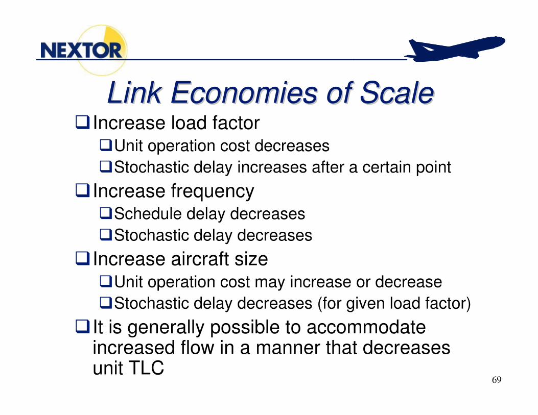
Link Economies of ScaleLink Economies of Scale�Increase load factor

�Unit operation cost decreases�Stochastic delay increases after a certain point

�Increase frequency�Schedule delay decreases�Stochastic delay decreases

�Increase aircraft size�Unit operation cost may increase or decrease�Stochastic delay decreases (for given load factor)

�It is generally possible to accommodate increased flow in a manner that decreases unit TLC

70

Implications of LOSImplications of LOS

��

�������

71

Implications of ESLImplications of ESL

������������ ���

72

Economies of IntegrationEconomies of Integration

� One-airline itineraries better than two-airline itineraries�Transaction costs�Connection costs�Consumer confidence

73

Disaggregate Choice ModelsDisaggregate Choice Models

�Model choices between discrete alternatives at individual level

�Assume choice behavior is utility maximizing

�Early applications in transportation, but now used (and abused) widely

74

UtilityUtility--Based ApproachBased Approach

�Assumes that individuals make rational choices

�Basis for choice is maximization of utility--level of satisfaction the traveler attains

�Utility is function of attributes of alternative, characteristics of choice maker/choice context

75

Decision TreeDecision TreeChoice Maker i

Characteristics Zi

Mode 1Attributes S1i

Mode 2Attributes S2i

Mode mAttributes Smi

U1=U1(Zi,S1i) U2=U2(Zi,S2i) Um=Um(Zi,Smi)

…

76

Aviation Choice AlternativesAviation Choice Alternatives

�Routes�Airline+Route�Airline�Airport�Airport+Airline�etc

77

Characteristics and AttributesCharacteristics and Attributes

� Traveler Characteristics�Income�Trip purpose�Travel party size�Frequent Flier

Affiliation

�Alternative Attributes�Fare�# of stops�Circuity�Frequency�Aircraft Size

78

LogitLogit ModelModel� Utility=Deterministic Utility+Stochastic

Utility

� Where �are independently, identically distributed�have a Gumbel distribution:

imimim SZV ε+= ),(

sim 'ε

)exp()( wim ewP −−=<ε

imimim VU ε+=

79

With these Assumptions:With these Assumptions:

�==

jij

iminiiniim V

VVVUUUP

)exp()exp(

)...)...max(( 11

�==

jij

imini V

VVVmchoicesiP

)exp()exp(

)...'( 1

80

Route Choice ModelRoute Choice Model

81

NAS Equilibrium Flow ModelNAS Equilibrium Flow Model

� Given the OD traffic predict equilibrium�Segment and airport pax flows�Airport delays

� Assess how equilibrium affected by increase in ORD capacity

82

Equilibrium Flow ModelEquilibrium Flow Model

Converge?SegPaxn+1

SegPaxn

Initial Values

DistanceSegPax0=OD Pax

HHIDelay0

Route Choice Model

DistanceSegPaxn

HHIDelayn

Choice Probabilities

Airport OD Traffic

SegPaxn+1 & Airport Traffic

EquilibriumLink & Airport

Traffic

System Update

SegPaxn+1

Delayn+1=f (Airport Pax n+1, Fixed effects)

No

Yes

n=0

n=n+1

Route Traffic

83

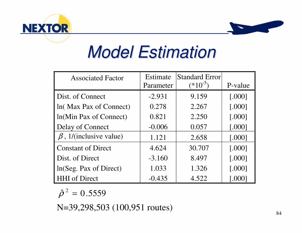
Hub Choice ModelHub Choice Model� Allocates OD Traffic to Segment Traffic—

Route (hub) Choice� Nested Logit Model

�Direct or one-stop connecting�Conditioned on connecting, choose the

connecting airport(hub)� Specification

odododdirect HHIbpaxDbdistDbcV 0302010 )ln( +++=

idioidioidioiod DelaybpaxbpaxbdistCbV 4/3/21, )ln(min)ln(max +++= −−

84

Model EstimationModel Estimation

5559.0ˆ 2 =ρN=39,298,503 (100,951 routes)

Associated Factor Estimate Parameter

Standard Error (*10-5) P-value

Dist. of Connect -2.931 9.159 [.000] ln( Max Pax of Connect) 0.278 2.267 [.000] ln(Min Pax of Connect) 0.821 2.250 [.000] Delay of Connect -0.006 0.057 [.000] β , 1/(inclusive value) 1.121 2.658 [.000] Constant of Direct 4.624 30.707 [.000] Dist. of Direct -3.160 8.497 [.000] ln(Seg. Pax of Direct) 1.033 1.326 [.000] HHI of Direct -0.435 4.522 [.000]

85

Policy ExperimentPolicy Experiment——ORD Delay ImprovementORD Delay Improvement

� Delay:

� Airport fixed delay effect improved:

4923.1' == ATLORD αα

8846.1=ORDα

ititi

iiit PaxCDelay εβαα +++= �=

)ln(**)ln( 1

30

10

86

Policy ExperimentPolicy Experiment——New Equilibrium FlowsNew Equilibrium Flows

� ORD: +998,014

� Other hubs: -728,603

� Net effect on the system: +269,410

� ORD attracts:� ¾ from

competing hubs

� ¼ from “direct”routes

-300

-100

100

300

500

700

900

1100

AT

LB

OS

BW

IC

LTC

VG

DC

AD

EN

DF

WD

TW

EW

RH

NL

IAD

IAH

JFK

LAS

LA

XLG

AM

CO

ME

MM

IAM

SP

OR

DP

HL

PH

XP

ITS

AN

SE

AS

FO

SLC ST

LT

PA

Connecting Airports

Cha

nge

d P

ax (

*100

0)

87

Policy ExperimentPolicy Experiment——New Equilibrium DelaysNew Equilibrium Delays

� ORD delay: reduce 12.0 (Flt/1000 Flt), about 27%

� Delays of other hubs also reduce

-13

-11

-9

-7

-5

-3

-1

1

AT

LB

OS

BW

IC

LTC

VG

DC

AD

EN

DF

WD

TW

EW

RH

NL

IAD

IAH

JFK

LAS

LAX

LGA

MC

OM

EM

MIA

MS

PO

RD

PH

LP

HX

PIT

SA

NS

EA

SF

OS

LC

ST

LT

PA

Connecting Airports

Cha

nge

d D

elay

(F

ligh

ts p

er 1

000

oper

atio

n)

88Q

P

D

S1

q1

p1S2

p2

q2

Effect of improvement at ORD on supply curve.

Depiction with Supply and Depiction with Supply and Demand CurvesDemand Curves

89Q

P

D

S1

q1

p1S2

p2

q2

Effect of improvement at ORD on supply curve.

Benefit from ImprovementBenefit from Improvement

90Q

P

D

S1

q1

p1S2

p2

q2

Effect of improvement at ORD on supply curve.

Benefit Assumed without Benefit Assumed without Demand ResponseDemand Response

91

Losses from Capacity Constraint: Losses from Capacity Constraint: Five Easy PiecesFive Easy Pieces

S’

S

D

Q

P

Potential users priced off system due to congestion.

Congestion costs to existing users.

Additional losses to existing users from failure torealize economies of scale.

Additional losses to users priced off as a result of congestion due to failure to realize economies of scale.

Additional losses to existing users from failure torealize economies of scale.

Potential users priced off system due to failure torealize economies of scale.

92

Optimal Pricing and InvestmentOptimal Pricing and Investment

� Given�Inverse Demand Function—P(Q)�User Cost Function—U(Q,K)�Supplier Cost Function—S(Q,K)

� Find�Optimal Q and K�Optimal user charge

93

Objective FunctionObjective Function

� Total user’s willingness to pay

� Total User Cost:� Total Supplier Cost:

�Q

dqqP0

)(

),( KQUQ ⋅−),( KQSQ ⋅−

94

First Order ConditionsFirst Order Conditions

� The user with the least willingness to pay should be willing to pay the cost his use will impose on other users the supplier, as well as on himself.

� This implies a charge of:� The savings in user cost from the marginal investment

should just offset the increase in supplier cost.

0)(

0),(),()(

),(),()(),(0

=∂∂+

∂∂⋅−=

∂∂

=−∂∂⋅−−

∂∂⋅−=

∂∂

⋅−⋅−= �

KS

KU

QKZ

KQSQS

QKQUQU

QQPQZ

KQSQKQUQdqqPKQZQ

),( KQSQS

QQU

Q +∂∂⋅+

∂∂⋅

95

Special CaseSpecial Case

QbU

KbK

QUKZ

aaUQP

baKQS

UKQU

KUQ

KUQ

KQ

QK

KQ

3/10

3

30

2220

20

20)

2(

Charge0))(1()(

),(

))(1(),(

02

02

��

���

�==+−=∂∂

−==−−+−

+=+=