The Economic Determinants of Crime: an Approach through ...fm · The Economic Determinants of...
32
The Economic Determinants of Crime: an Approach through Responsiveness Scores Giovanni Cerulli 1 , Maria Ventura 2 , and Christopher F Baum 3,4,5 1 CNR–IRCrES 2 STICERD, London School of Economics 3 Department of Economics, Boston College 4 School of Social Work, Boston College 5 Department of Macroeconomics, DIW Berlin Abstract Criminality has always been part of human social interactions, shaping the way peoples have constructed states and legislation. As social order became a greater concern for the public authorities, interest in investigating incentives pushing individuals towards engaging in illegal activities has become a central issue of the political agenda. Building on the existing literature, this paper proposes to focus on a few primary determinants of crime, whose effect is in- vestigated using a Responsiveness Scores (RS) approach performed over 50 US states during the period 2000–2012. The RS approach allows us to account for unit heterogeneous response to each single determinant, thus paving the way to a more in-depth analysis of the relation between crime and its drivers. We attempt to overcome the limitations posed by standard regression methods, which assume a single coefficient for all determinants, thus contributing to the literature in the field with stronger evidence on determinants’ effects and the geographical patterns of responsiveness scores. Keywords: Crime, Incentives, Responsiveness Scores JEL Classification: K42, J24, P46 1
Transcript of The Economic Determinants of Crime: an Approach through ...fm · The Economic Determinants of...

The Economic Determinants of Crime:
an Approach through Responsiveness Scores
Giovanni Cerulli1, Maria Ventura2, and Christopher F Baum3,4,5
1CNR–IRCrES
2STICERD, London School of Economics
3Department of Economics, Boston College
4School of Social Work, Boston College
5Department of Macroeconomics, DIW Berlin
Abstract
Criminality has always been part of human social interactions, shaping the
way peoples have constructed states and legislation. As social order became a
greater concern for the public authorities, interest in investigating incentives
pushing individuals towards engaging in illegal activities has become a central
issue of the political agenda. Building on the existing literature, this paper
proposes to focus on a few primary determinants of crime, whose effect is in-
vestigated using a Responsiveness Scores (RS) approach performed over 50 US
states during the period 2000–2012. The RS approach allows us to account for
unit heterogeneous response to each single determinant, thus paving the way
to a more in-depth analysis of the relation between crime and its drivers. We
attempt to overcome the limitations posed by standard regression methods,
which assume a single coefficient for all determinants, thus contributing to the
literature in the field with stronger evidence on determinants’ effects and the
geographical patterns of responsiveness scores.
Keywords: Crime, Incentives, Responsiveness Scores
JEL Classification: K42, J24, P46
1

1 Introduction
In the last decades, crime has been a critical societal issue in the United States, and
a topic of intensive research both in economics and other social sciences. After a
steady and worrying rise of crime rates between the 1960s and 1980s, trends have
been moving the opposite way since the 1990s (Kearney et al. (2014)).
There is no single cause identifying the different levels of crimes over time, as a
number of determinants, often interacting, contribute to their variations. These may
range from social to geographical and historical causes, and events whose effect is only
indirect, but equally strong. For instance, Levitt & Dubner (2005) argue that the
legalization of abortion throughout the country in 1973 has been critical in reducing
crime rates in the following generation, and attribute this to the decrease in the birth
rates among the most disadvantaged or unstable social categories.
Socioeconomic factors also play a major role by determining, for instance, the
inclusion within one of these social categories, but also, as discussed in this paper,
establishing incentives for engaging in crime. The issue with this type of setting is
that most of the previous literature in the field have mainly analysed each driver
individually, without necessarily providing a global account of the phenomenon. For
instance, Lochner (2004) focused on the role of education, while Fowles & Merva
(1996) focus on the effect of changes in the distribution of wage income. Although an
intensive knowledge of each single factor can definitely offer some critical insight, we
believe that gathering the main determinants and observing how those interact in an
inclusive context should result in more realistic scenarios that would reflect society in
all its aspects. Clearly, performing a multiple regression, with the factors of interest
as independent variables, would be the most common way to proceed in order to
respond to the research question and look at possible causality links. However, this
standard approach contains the obvious limitation of assuming that coefficients are
identical across units and time, thus ignoring potential heterogeneity in the impact
of the factors, whose effects are likely to vary according to the geographical and
historical framework.
Therefore, we choose instead to adopt the method of responsiveness scores, whose
successful application by Cerulli (2014) in the field of technological innovation has
raised the possibility for its use in different fields. Responsiveness scores are based
on an iterated Random Coefficient Regression model (Wooldridge (2010)) for each
unit and for each factor. A more detailed and technical description of the underlying
2

econometrics follows. The main advantage of this technique is that it relaxes the
classic assumption that each observation of the population has the same slope, thus
allowing for idiosyncratic responses. Moreover, among the other features, it makes
it possible to analyze factor accumulation returns, for the investigation on both the
same factor and a cross-partial effect of other determinants. Hence, our aim is to
enhance the existing literature by adding a study of the overall dynamics of the main
drivers of crime, as identified and discussed by other authors, in all their complexity,
heterogeneity, and interaction.
The rest of the paper is organized as follows. Section 2 presents an overview of
the theoretical framework, while Section 3 presents a brief explanation of the method
of responsiveness scores and describes the data. Section 4 shows the main results and
provides a rationale, based on past research, for the obtained outcomes while Section
5 concludes.
2 Theoretical background of the determinants of
crime
The causes of crime have been widely studied by social sciences, with economic deter-
minants acquiring greater relevance during the last decades. Although the analysis
of the effect of income on delinquency was not new to the field (e.g., Fleisher (1966)),
this stream of modern literature was pioneered by Becker (1968). In his seminal pa-
per, he presents the criminal’s choice, intended as the main trigger of the “supply of
offenses,” as a standard microeconomic problem of expected utility: the individual
chooses whether to commit a crime by comparing its expected benefits with its costs,
which also can include the loss of an outside option, usually represented by income
from a legal, and less risky, activity. He also introduces the theme of punishment
of crime, which enters the problem both in the forms of probability of being caught
and magnitude of the penalty. Ehrlich (1973) refines and extends this model, and
gives a greater twist to the discussion of the responsiveness of individuals to economic
incentives and to their interaction. In this context, many other factors besides indi-
vidual income can be included in the analysis of the determinants of crime, as they
modify people opportunities in legal activities, and therefore their expected returns
from engaging in offenses. Here, we choose to consider six main drivers analyzed in
previous studies which are likely to be correlated to other omitted factors. They are:
3

• Educational attainment;
• Employment level;
• Wage income;
• Income inequality;
• Public expenditure on police;
• The presence of foreign born population.
We proceed by discussing some of the related literature for each of these factors.
Education can impact the incidence of crimes in several ways. Machin et al.
(2011), among others, extensively discuss three main channels. Through income ef-
fects, education increases expected wages, and therefore the returns from legitimate
work, increasing the opportunity cost of crime. Following this idea, most scholars
would predict a decrease in criminal activity for an increase in education, although
Levitt & Lochner (2001) find that certain mechanical knowledge and related disci-
plines can improve chances in the criminal world. Resources allocated to education
also create time constraints that should work in keeping teenagers away from com-
mitting offenses. Witte & Tauchen (1994) find that greater time spent in school is
correlated with a lower probability of criminal activity. Moreover, a stream of liter-
ature also associates greater education with higher life satisfaction, as in Oreopoulos
(2007) and Lochner (2004) finding that higher levels of education increase patience
and risk aversion, thus lowering crime.1 Usher (1997) considers a fourth channel, a
civic externality of education, which is assumed to affect one’s willingness to com-
mit an offense. In general, we would therefore expect a negative relation between
educational attainment and crime.
Labor market conditions have also been widely used to motivate different incidence
of crime. Although employment status has been prevalent in the early literature, with
Fleisher (1963) establishing a positive effect of unemployment on delinquency, modern
works have rather focused on the pecuniary aspect of labor market. Gould et al. (2002)
remark that, as employment is highly cyclical, it can hardly explain a long-term trend
in crime, as observed in the United States. Moreover, Gumus (2003) distinguishes
between short-term and long-term effects of unemployment, and concludes that while
1The attitude toward risk is a factor that Becker (1968) also takes into consideration in his model.
4

after being unemployed for a short period people tend to look for another job, a long
spell of unemployment increases the likelihood of criminal activity. The wage from
legal activities matters both as a component of income, and as the opportunity cost of
criminal actions. Concerning the first aspect, Buonanno (2003) highlights that both
the income of the offender and that of the victim represent relevant factors, as the
first is a cost while the second an incentive to commit crimes, thus leading to expect
opposite signs of their effects.
Different studies have also led to believe that income inequality plays a critical
role in determining crime levels. Buonanno (2003) highlights that income inequality
can be thought as a measure of the differential between legal and illegal payoffs
and Imrohoroglu et al. (2006) identify it as one of the variables having the greatest
effect on the crime rate. As explained by Kelly (2000), the direct effect of inequality
is to juxtapose those with low returns from their legal activities and people with
considerably higher wealth. A second consequence of inequality is explicated by the
strain theory of Merton (1938), who argues that because of the same juxtaposition
of social classes, frustration of the poorest individuals could represent a triggering
motive for criminal activity. In both cases, the impact of inequality should then lead
to higher crime rates.
Police presence and public expenditure in protection has also claimed a relevant
impact on crime. The topic is extensively discussed by Levitt & Dubner (2005):
although recognizing that there may be simultaneity bias, as police presence action
affects crime trends, but also a higher crime rate will call for higher police protection.
They provide some interesting evidence of an inverse effect of police on crime by
using exogenous changes in the number of police around the time of elections to find
that additional police can lower the crime rate. On the other hand, by looking at
the significant crime decline of the 1990s in the United States, they also show that
innovative police strategies had a more limited effect. Draca & Machin (2015) note
that the effect of policing is oriented towards a deterrence mechanism, which enters
the framework outlined in Becker (1968) by decreasing the expected returns from
crime. Di Tella & Schargrodsky (2002) partly confirm this suspected negative effect
by using a natural experiment to find the effect of larger police forces on car theft.
Finally, Buonanno (2003) highlights the importance of social interactions and
social networks among the determinants of crime. This raises the issue of immigra-
tion, whose link with criminality has always been rather controversial. Camarota
5
& Vaughan (2009) stress several problems in terms of data collection and contrary
results in the previous literature. Also, the answer to this question is likely to change
according to the geographical area, its economic characteristics, the composition of its
immigration pool, and their integration with the native population. Due to all these
challenges, the literature on migration and crime is not as extensive as on the other
determinants. Nevertheless, at least in the United States, racial inequality is still a
dominant feature, and it has been widening with the Great Recession (Kochhar &
Fry (2014)). This suggests an intrinsic disadvantage of being “different” that, again
as in Merton (1938), might be manifested as a higher propensity to engage in criminal
activities.
3 Data and methodology
3.1 Data and variables description
The dataset is a panel constructed for 50 US states2 for the period 2000–2012. Data
for the demographic and microeconomic variables are an elaboration from the Amer-
ican Community Survey (ACS) microdata available from IPUMS USA, and we used
the 2010 Consumer Price Index to deflate nominal measures. Measures of public
expenditure on police forces have been retrieved from the US Census Bureau Govern-
ment Finances section, and the Gini Index for the states is calculated by the Economic
Department of Houston State University. The outcome variable is represented by a
crime rate of a state s in a given year t. This is constructed as
crimest =V Cst + PCst
Popst
where V Cst is the number of violent crimes3 for the unit observation and PCst the
number of property crimes4 for the same, and the denominator Popst the total pop-
ulation of the state at that time. Data on crime in the US is available through the
FBI Uniform Crime Reporting System database, and it has been aggregated from
2Hawaii is not included as it doesn’t participate to the FBI Uniform Crime Reporting Program.We include the District of Columbia (DC).
3The FBI UCR program defines “Violent crimes” as “those offenses which involve force or threatof force”, including murder and nonnegligent manslaughter, forcible rape, robbery, and aggravatedassault (U.S. Federal Bureau of Investigation (2016b)).
4“Property crimes” are those with the object of “taking of money or property, but there is noforce or threat of force against the victims”, and include burglary, larceny-theft, motor vehicle theft,and arson (U.S. Federal Bureau of Investigation (2016a)).
6

the agency level data. For each state and year of observation, we consider six factor
variables in order to construct responsiveness scores:
• Education: average school attainment for the population;
• Employment : employment rate calculated as ratio of employed workers over
working age population (15–65 years old);
• Police: total amount of state government expenditure in police protection;
• Inequality : as represented by the Gini coefficient of income inequality;
• Wage: average wage and salary income for the population;
• Foreign born: ratio of foreign born over total population.
All the factor variables have been lagged one year, in order to account for possible
delayed effects. Moreover, an indicator for the political orientation of the state (red or
blue) is used as a control variable. Later in the analysis, measures of total household
income, and a diversity index constructed as in Ottaviano & Peri (2006)5 are also
used in order to rank the states and investigate the aforementioned effects for given
categories.
3.2 The responsiveness scores approach
As explained above, the investigation of the socioeconomic determinants of crime is
not new to the literature. In this paper, however, we propose a new type of analysis
based on the Responsiveness Scores technique as proposed by Cerulli (2014, 2017).
The main advantage of this approach is that it allows for heterogeneous responses of
the macro units of observation to the factor variables. In what follows, we set out a
concise methodological account of this method.
5The index is constructed as the probability that two individuals that are randomly drawn from
the population of the state are born in the same country: DIst = 1−M∑i=1
(CoBist
TPst
)2, where CoBist
is the number of residents born in country i ; TPst is the total population of the state; and M is thenumber of different cultural groups that are potentially present in the state.
7

Responsiveness scores (RS) measure the change of a given outcome y when a given
factor xj, (j = 1, . . . , Q) changes, conditional on the other (Q− 1) factors:
x−j = [x1, . . . , xj−1, xj+1, . . . , xQ]. (1)
Algebraically, it is the derivative of y on xj, given x−j, when one allows for each
observation to have its own responsiveness score. We assume that x−j is a vector of
all exogenous variables. RS are obtained by an iterated random–coefficient regression
(RCR), whose basic econometrics can be found in (Wooldridge 2010, pp. 141–145).
The calculation of RS follows this simple protocol:
1. Define y, the outcome (or response) variable.
2. Define a set of Q factors thought of as affecting y, and indicate the generic
factor with xj.
3. Define a RCR model linking y to the various xj, and extract a unit–specific
responsiveness effect of y to all set of factors xj, with j = 1, . . . , Q.
4. For the generic unit i and factor j, indicate such effect as bij and collect all of
them in a matrix B.
5. Finally, aggregate by unit (row) and/or by factor (column) the E(bij|xi,−j) thus
getting synthetic unit and factor responsiveness measures.
Analytically, a RS is the “partial effect” of a factor x in a RCR (Wooldridge, 1997;
2003; 2004). Indeed, for each j = 1, . . . , Q, define a RCR model of this kind:yi = aij + bijxij + ei
aij = γ0 + xi,−jγ + uij
bij = δ0 + xi,−jδ + vij
(2)
where ei, uij and vij are freely correlated error terms with:
E(ei|xi,−j;xij) = E(uij|xi,−j;xij) = E(vij|xi,−j;xij) = 0 (3)
It is easy to see that the regression parameters, aij and bij, are both non-constant
as they depend on all the other inputs x except xj due to the definition of the vector
8

xi,−j). Observe that δ0 and γ0 are, on the contrary, constant parameters. According
to this model, we can define the regression line as:
E(yi|xij,xi,−j) = E(aij|xi,−j) + xij · E(bij|xi,−j) (4)
Given this, we define the responsiveness effect of xij on yi as the derivative of yi
respect to xij, that is:
∂
∂xij[E(yi|xij,xi,−j)] = E(bij|xi,−j) (5)
where E(bij|xij,xi,−j) is the partial effect of xij on yi. We can repeat the same
procedure for each xij (with j = 1, ..., Q) – so that it is eventually possible to define,
for each unit i=1,..., N and factor j = 1, ..., Q, the N × Q matrix B of the partial
effects as follows:
B =
E(b11|xi,−j) . . . E(b1Q|xi,−j)
... E(bij|xi,−j)...
E(bN1|xi,−j) · · · E(bNQ|xi,−j)
(6)
If all variables are standardized with zero mean and unit variance, partial effects are
beta–coefficients, thus independent of the unit of measurement. As such, they can be
compared with each other and summed6.
In a cross–section data setting, Ordinary Least Squares (OLS) provides consistent
estimation of each bij within this regression7
yi = γ0 + xi,−jγ + (δ0 + x−jδ)xij + xij(xi,−j − x−j)δ + ηi
ηi = uij + xijvij + ei(7)
where x−j is the vector of the sample means of xi,−j.
6As beta-coefficients are measured in standard deviation units, they can be compared. Themeaning of a beta-coefficient is straightforward: suppose that in a regression of y on x the betais found to be equal to 0.3, then it means that one standard deviation increase in x leads to a 0.3standard deviation increase in the predicted y with all the other variables in the model held constant.
7Indeed, OLS estimates are consistent as for each j = 1, . . . , Q we have E(ηi|xij) = E(uij |xij) +xij ·E(vij |xij) +E(ei|xij) = 0. However, as ηi is clearly heteroskedastic, a robust VCE is necessaryto produce consistent standard errors.
9
Once these regression parameters are estimated, we can obtain an estimate of the
partial effect of factor xj on y for unit i as:
E(bij|xi,−j) = δ0 + xi,−j δ (8)
By repeating this procedure for each unit i and factor j, we can finally obtain B, i.e.
the estimation of matrix B.
When a longitudinal dataset is available, the estimation of B can be obtained
either by using random-effects or fixed-effects estimation of the following panel data
regression:
yit = γ0 + xi,−j,tγ + (δ0 + x−j,tδ)xijt + xijt(xi,−j,t − x−j,t)δ + αi + ηit (9)
where the added parameter αi represents a unit–specific effect accounting for unob-
served heterogeneity. In particular, fixed–effect estimation, by allowing for arbitrary
correlation between αi and ηit, can mitigate a potential endogeneity bias due to mis-
specification of previous equation and measurement errors in the variables considered
in the model (Wooldridge 2010, pp. 281–315). As such, a panel dataset may allow
for more reliable estimates of the responsiveness scores than OLS estimates on a
cross-section.
If the variables are standardized, eq. (9) becomes:
yit = γ0 + xi,−j,tγ + δ0xijt + xijt · xi,−j,tδ + αi + ηit (10)
which simplifies the formula.
Finally, following Eq. (8), the variance of the propensity score can be found to be
equal to:
V ar[E(bij|xi,−j)
]= V ar(δ0) + x2
i,−jV ar(δ) + 2 · xi,−j · Cov(δ0; δ) (11)
that allows us to compute, for each single score, the statistical significance at the
three commonly considered levels of 1% , 5%, and 10%. For the sake of simplicity, we
report here for each factor just a “rate of significance”, i.e. the share of responsiveness
scores significant at least at the 10% level.
10

4 Results
Table 1 shows that the R-squared statistic is particularly high for all factors, ranging
from 0.69 to 0.73, with a mean of 0.71. The same is true for the category of property
crimes, although the average R-squared drops to about 0.49 when using the ratio of
violent crimes over population as the dependent variable. Nevertheless, this shows
a reasonable goodness of fit, so we are confident that our coefficients take account
of important correlations in the data. Moreover, the significance rate is particularly
high (93%) for the factor Police and around 50% for Education, Foreign born and
Inequalities. On the other hand, the factors Employment and Wage exhibit lower
shares of scores significant at least at the 10% threshold (23% and 29% respectively).
When separately analyzing the two types of crimes, significance rates are not dissim-
ilar from the aggregate ones in the case of Police and Foreign born, while generally
more elevated for violent crimes rather than property crimes (with the exception of
Inequality).
Dependent variable Mean R2 Factors Significance rate
Total crime 0.71
Education 0.55Employment 0.23
Police 0.93Inequality 0.47
Wage 0.28Foreign born 0.54
Violent crime 0.49
Education 0.62Employment 0.39
Police 0.92Inequality 0.33
Wage 0.42Foreign born 0.54
Property crime 0.71
Education 0.55Employment 0.19
Police 0.92Inequality 0.47
Wage 0.31Foreign born 0.52
Table 1: Summary table for the R-squared statistics and the Significance rate.
We proceed by presenting our results in the following order. First, we comment
on the distribution of the responsiveness scores and on some descriptive statistics;
second, we move to a graphical study of the factor returns, in order to assess whether
11

01
23
4
-1 -.5 0 .5 1 1.5
Education Employment
Police Inequalities
Wage Foreign born
Figure 1: Distribution of the responsiveness scores over the period 2000-2012.
different levels of a factor can influence the responsiveness of crime rates. Third, we
perform a brief analysis by aggregating our observations in sub–national units; and
finally, we disaggregate our crime measure in order to account for differential effects
depending on the type of crime (i.e., property and violent).
4.1 Distribution of the responsiveness scores
The responsiveness scores approach allows to perform a series of additional analyses,
ranging from the representation of their distributions and basic descriptive statistics
to the study of the single idiosyncratic responses to the factors. Figure 1 shows the
first analysis, regarding the distribution of the responsiveness scores for the different
factors, while Figure 2 shows the time trends for the annual scores averages. The
former allows us to rank the factors according to the magnitude of their effects. We
can also assess the volatility of this effect by looking at the standard deviation.
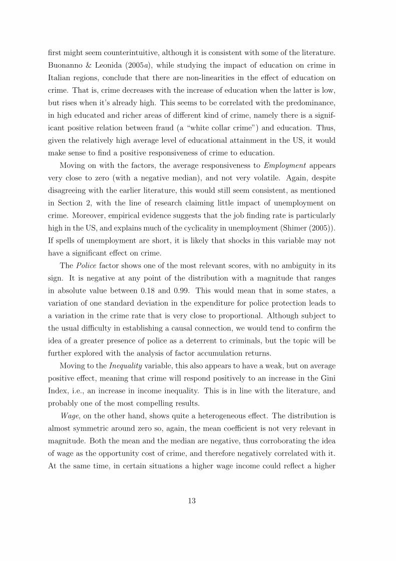
We find that Education has, on average, a weak but clearly positive effect. This at
12
first might seem counterintuitive, although it is consistent with some of the literature.
Buonanno & Leonida (2005a), while studying the impact of education on crime in
Italian regions, conclude that there are non-linearities in the effect of education on
crime. That is, crime decreases with the increase of education when the latter is low,
but rises when it’s already high. This seems to be correlated with the predominance,
in high educated and richer areas of different kind of crime, namely there is a signif-
icant positive relation between fraud (a “white collar crime”) and education. Thus,
given the relatively high average level of educational attainment in the US, it would
make sense to find a positive responsiveness of crime to education.
Moving on with the factors, the average responsiveness to Employment appears
very close to zero (with a negative median), and not very volatile. Again, despite
disagreeing with the earlier literature, this would still seem consistent, as mentioned
in Section 2, with the line of research claiming little impact of unemployment on
crime. Moreover, empirical evidence suggests that the job finding rate is particularly
high in the US, and explains much of the cyclicality in unemployment (Shimer (2005)).
If spells of unemployment are short, it is likely that shocks in this variable may not
have a significant effect on crime.
The Police factor shows one of the most relevant scores, with no ambiguity in its
sign. It is negative at any point of the distribution with a magnitude that ranges
in absolute value between 0.18 and 0.99. This would mean that in some states, a
variation of one standard deviation in the expenditure for police protection leads to
a variation in the crime rate that is very close to proportional. Although subject to
the usual difficulty in establishing a causal connection, we would tend to confirm the
idea of a greater presence of police as a deterrent to criminals, but the topic will be
further explored with the analysis of factor accumulation returns.
Moving to the Inequality variable, this also appears to have a weak, but on average
positive effect, meaning that crime will respond positively to an increase in the Gini
Index, i.e., an increase in income inequality. This is in line with the literature, and
probably one of the most compelling results.
Wage, on the other hand, shows quite a heterogeneous effect. The distribution is
almost symmetric around zero so, again, the mean coefficient is not very relevant in
magnitude. Both the mean and the median are negative, thus corroborating the idea
of wage as the opportunity cost of crime, and therefore negatively correlated with it.
At the same time, in certain situations a higher wage income could reflect a higher
13

-.6-.4
-.20
.2.4
2001 2004 2007 2010 2013
Education Employment
Police Inequality
Income Foreign population
Figure 2: Timepaths of the responsiveness scores for the period 2000–2012.
household income, or income per capita. In this case, as explained by Buonanno
(2003), there could be a higher potential gain (the victims’ income) from certain
kinds of crime, and specifically property crime (Fleisher (1966)).
Finally, crime has a predominantly positive responsiveness to the share of Foreign
born. Although this is true on average, and for most of the observations, for a small
part of them the opposite is true. We conclude that the direction of the impact of
immigrants on crime critically depends on the level of immigrants’ integration among
the native population. This, on turn, could reflect different levels of education and
income within the foreign community. Moreover, as mentioned in Section 2, a big
part of the story may be the dominant incidence of poverty among immigrants, and
especially non-white. This inevitably brings us back to the issue of income inequality,
to which this share of the population tends to be the most affected.
14

4.2 Returns to scale
We move now to a deeper analysis of the phenomenon, using a particular feature
enabled by the use of the responsiveness scores approach. One useful aspect is the
investigation of factor accumulation returns, which produces some interesting results.
As shown in Figure 3, where the responsiveness score for the first factor is plotted
-.50
.5R
S fo
r 'E
duca
tion'
12 13 14 15Education
-.50
.5R
S fo
r 'E
duca
tion'
0 .1 .2 .3 .4 .5Diversity Index
Figure 3: Factor accumulation returns for Education.
over the average years of schooling and the diversity index for each state, Education
shows stable returns for the intermediate range, while decreasing at the extremes.
This would suggest that an increase in the average level of education, when this is
relatively low, brings a less than proportional increase in crime, while implying a
decrease in the crime rate for very high levels of education. With reference to the
above mentioned work by Buonanno & Leonida (2005b), this suggests a further non-
linearity in the responsiveness to the education level. What is even more striking is
the result achieved from plotting the responsiveness to Education and a measure of
cultural diversity (Ottaviano & Peri (2006)). To investigate this, we check whether
15

different levels of diversity interact with the responsiveness to education. The relation
is unambiguously negative, with the effect of education on crime decreasing and soon
becoming negative for higher levels of the diversity index. At the same time, if
the diversity index only proxies for the amount of foreign born, this could also be
a sign of the higher level of schooling attainment among the most disadvantaged
social categories (which, as mentioned before, often happen to be the non-whites):
increased education for this share of the population, where the initial level would most
likely be lower than average, and which, because of its economic condition, might be
particularly engaged in illegal activities, could therefore lead to reduced crime rates.
-.4-.2
0.2
.4.6
RS
for '
Em
ploy
men
t rat
e'
.6 .65 .7 .75 .8 .85Employment rate
-.4-.2
0.2
.4.6
RS
for '
Em
ploy
men
t rat
e'
.5 .55 .6 .65 .7Inequalities
Figure 4: Factor accumulation returns for Employment.
The representation of the returns for Employment (Figure 4), which appear to
be bell-shaped, is also of interest. The responsiveness score stays negative for most
of the levels of the employment rate, but begins with increasing returns, reaches a
peak where employment actually seems to increase crime, and then decreases again
to negative values.
16

Therefore, the greatest effects in reducing crime rates appear to be concentrated
where employment is low, and thus an increase brings a sensible change in the op-
portunity cost of crime, or where this is particularly high: probably high enough to
dissuade criminal activity. We explore a different side of the story by plotting the
responsiveness to Employment on the levels of income inequality, as expressed by
the Gini coefficient. This time, the relation is clearly positive, implying a greater
responsiveness to the employment rate with the increase of inequality. More specifi-
cally, the effect of employment on crime is negative but decreasing in absolute value
for low levels of income inequality, but it becomes positive and increasing for higher
values of the Gini index. When wealth is unevenly distributed within the society,
even increases in employment do not benefit the poor as much as they benefit the
rich, therefore triggering social tensions and incentives for criminality.
Accumulation returns of Police are not readily interpreted, but they nevertheless
present the relevant feature of being increasing (or, in absolute value, decreasing)
after a certain threshold. The first panel of Figure 5 is telling us that, although a
higher presence of police has a negative impact on crime rate (as specified above,
along the whole distribution), the responsiveness still suffers from decreasing returns
to scale. Crime rates decrease less than proportionally with higher expenditures on
police protection. Interestingly, this is not the case for the lowest level of expenditure
where returns are increasing in magnitude, therefore suggesting that the presence of
police is still so low that even a slight increment has a strong negative effect on crime.
Overall, this seem to be a reassuring result. As pointed out by Levitt & Dubner
(2005), higher expenditures on police protection can lower criminality, but if this is
not paired with other complementary measures, this turns not to be necessarily the
most efficient way to foster social order.
The graphs for the returns of Inequality and Wage (Figure 5) do not tell us that
much: they are generally stable and flat, with the exception of a decreasing range for
Inequality and a slight bump in the responsiveness to Wage for higher values.
Finally, the responsiveness score to the Foreign born (Figure 5) variables also
shows relevant behavior. This stays very stable and close to zero when the share
of foreign population stays below 20%, but it grows steeply until values of one and
beyond when Foreign born overtakes this threshold. The fact suggests that integra-
tion is not playing a strong role in this model. Consequently, a higher percentage
of immigrants tends to exacerbate crime, with changes in responsiveness that are
17

more than proportional. Again, the fact that foreign born population is on average
more economically disadvantaged brings us back to the economic components of the
analysis, which in turn might make the foreign born more prone to engage in crime.
-1-.8
-.6-.4
-.2R
S fo
r 'po
lice'
0 5000000 1.00e+07 1.50e+07Police expenditure
-.6-.4
-.20
.2.4
RS
for '
Gin
i ind
ex'
.5 .55 .6 .65 .7Gini Index
-.4-.2
0.2
.4R
S fo
r 'W
age'
150000 200000 250000 300000Wage Income
-.50
.51
1.5
RS
for '
Fore
ign
born
'
0 .1 .2 .3Foreign born
Figure 5: Factor accumulation returns for Police, Wage, Inequality and Foreign born.
4.3 Geographical patterns
Another interesting feature that we can employ by working with responsiveness scores
is the possibility of using the idiosyncratic effect of the factor variables on the inde-
pendent one at the individual unit (or state) level. This allows us to investigate
connections and interactions among factors through different aggregations of these
units. We performed a geographical analysis by dividing our sample into the four
Census regions (West, Midwest, Northeast and South) thus evaluating their average
responsiveness scores over the sample period contrasted with the overall mean for the
US. As we can see in Figure 6, the subsets present behavior that are very similar to
the macro trends except for two considerable outliers. First of all, we can easily see
18
from the graph that the Midwest area, with its particularly high responsiveness score
for Education, is the one raising the average and making the overall effect positive,
as it otherwise would be negative for the other regions). Second, the West has a clear
spike at the Foreign born corner, that points to a much greater response of crime
to immigrants for this area. The questions that comes naturally is: what might be
creating these anomalies?
Exploring our data, we find that 75% of the states in the Midwest are ranked
below average when units are ordered according to their average Gini coefficient,
i.e. income tends to be more fairly distributed. On the basis of the literature, a
possible hypothesis would therefore be that, suffering less from inequalities, crimes
that are mainly due to resentment and social tensions (Merton (1938)), as violent
crimes, are less common, with possibly more property crime. According to Buonanno
& Leonida (2005b) and Abdullah et al. (2015) education has the effect of reducing
income inequality. Thus, a lower Gini index could be signalling for higher education
level, which in turn points to a greater likelihood of committing property crimes.
As for the case of the West region, performing a similar exercise, all of the eleven
states in the subsample appear in the second half of the ranking, with eight being
among the lowest ten. It is clear that we are now considering the poorest units of the
sample: we could for instance presume a hostile attitude of the natives, because of
the adverse economic situation, towards immigrants, that makes crime more reactive
to the share of foreign born. Another possibility, is that being the states relatively
poor, new immigrants will more likely be poor as well, and typically poorer than the
natives, thus triggering social conflict and then crime.
As a last step, we also report the same kind of results for the ten states with the
highest crime rate (Figure 7) as well as for the lowest ten (Figure 8). Except for a few
states departing from the mean, the two graphs are characterized by distinct shapes.
For the units with the highest crime rates, the values are very similar to those of the
overall US average, with a particular high incidence of the Foreign born factor. On the
other hand, for the states with low crime rates, the responsiveness to Education and
Inequality is on average extremely high, while the effect of Police tends to be lower
in magnitude. While the first fact could be explained through economic differences,
the second set of findings is less comprehensible. We could suppose that, where the
crime level is low, changes in Education and Inequality produce a greater shock to the
dependent variable, thus causing responsiveness to be higher. At the same time, as
19

Figure 6: Incidence of factors by regions.
illegal activities are not predominant, an increase in the expenditure for police does
not cause crime to fall as much as it would be in higher crime contexts. Moreover,
the crime rate could already be low because of the prevalence of policing which lowers
the effect of additional units of the same factor.
Figure 7: Incidence of factors in the highest 10 crime rate states.
4.4 Violent vs. Property crimes
We move now to testing whether our hypotheses on the existence of different effect
depending on the type of crime are actually confirmed by the data. The FBI Uniform
20

Figure 8: Incidence of factors in the lowest 10 crime rate states.
Crime Reports program (U.S. Federal Bureau of Investigation (2010b,a)) only distin-
guishes crimes according to the type of offense: violent crime or property crime. For
the rest of the analysis, we will assume that the category of “white collar crimes” are
mostly included in property crimes8.
We define two new variables vcrimest and pcrimest, which will be our outcomes
of interest in this section. They follow the same construction of the previous crimest
such that:
crimest = vcrimest + pcrimest =V Cst
Popst+PCst
Popst(12)
We proceed by performing the same type of analysis with regard to the aggregate
variable. The distributions of responsiveness scores look quite different for the two
variables, as shown in Figure 13 in the Appendix, with the one for property crime
generally much more volatile than for violent crimes. As a matter of fact, most of
the factors’ responsiveness scores are centered around zero for violent crimes, which
can be thought as less likely to be responsive to economic conditions. On the other
hand, property crime exhibits a positive correlation with education, confirming the
intuition explained above for white collar crimes, as well as an inverse relation with
employment.
Time trends (Figure 9) also shows peculiar paths when differentiating the two
8“White collar crimes” are defined (U.S. Federal Bureau of Investigation (2010c)) as ”thoseillegal acts which are characterized by deceit, concealment, or violation of trust and which are notdependent upon the application or threat of physical force or violence” and specifies that “individualsand organizations commit these acts to obtain money, property, or services; to avoid the paymentor loss of money or services; or to secure personal or business advantage.”
21

aspects. While property crimes’ responsiveness scores generally appear to have an
almost constant mean over time, violent crime varies more across years. In particular,
all factors but employment show decreasing trends. Moreover, responsiveness scores
for violent crime are in general smaller in absolute value.
-.50
.5
2001 2004 2007 2010 2013
A
-.50
.5
2001 2004 2007 2010 2013
B
Education Employment
Police Inequality
Income Foreign population
Figure 9: Time trends for (a) violent crime; (b) property crime.
We also repeated the exercise on both variables for the factor returns analysis.
First, we look at the Education factor, whose graphical representation is in Figure
10. Plotting the responsiveness scores for Education over the average years of the same
factors produces graphs that are similar in their slightly decreasing shape, but that
also present a crucial difference. For violent crimes, responsiveness is always negative
and increasing in absolute value for the highest levels of education. However, they
turn from positive to negative in the case of property crimes. In other words, in the
case of property crime, increasing education from a low level of schooling increases
crime, while moving to higher average education the effect has the opposite sign.
Again, this could be taken as evidence of the presence of white collar crimes within
22

our broader category: skills acquired through education are initially complementary
to crimes as fraud or embezzlement. However, the benefits that very high levels
of education can provide increase the opportunity cost of committing crime, thus
inverting the tendency.
Moreover, when we examine the relationship between scores for education and
cultural diversity for the two categories of crime, it is clear that the overall decreasing
correlation shown in Section 4.2 is mainly driven by violent crimes. This clear pattern
would suggest that, for increasing levels of cultural diversity, raising education has a
greater effect on reducing violent crime, while its impact on property crime is smaller.
-1-.5
0.5
RS
for '
Edu
catio
n'
12 13 14 15Education
A
-1-.5
0.5
RS
for '
Edu
catio
n'
12 13 14 15Education
B
-1-.5
0.5
RS
for '
Edu
catio
n'
0 .1 .2 .3 .4 .5Diversity Index
-1-.5
0.5
RS
for '
Edu
catio
n'
0 .1 .2 .3 .4 .5Diversity Index
Figure 10: Factor accumulation returns for Education.
Moving now to the returns for Employment, Figure 11 presents us with a few
points of interest, although the differences are not as significant as for Education.
The inverse U-shaped relation we have seen above is now particularly evident in the
case of property crimes, suggesting an increase in responsiveness due to the presence
of more skilled and able workers, and a following reduction, possibly connected to a
23
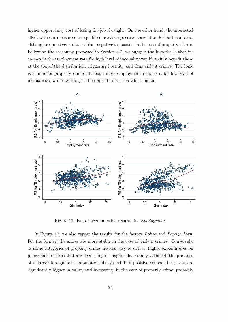
higher opportunity cost of losing the job if caught. On the other hand, the interacted
effect with our measure of inequalities reveals a positive correlation for both contexts,
although responsiveness turns from negative to positive in the case of property crimes.
Following the reasoning proposed in Section 4.2, we suggest the hypothesis that in-
creases in the employment rate for high level of inequality would mainly benefit those
at the top of the distribution, triggering hostility and thus violent crimes. The logic
is similar for property crime, although more employment reduces it for low level of
inequalities, while working in the opposite direction when higher.
-.4-.2
0.2
.4.6
RS
for '
Em
ploy
men
t rat
e'
.6 .65 .7 .75 .8 .85Employment rate
A
-.4-.2
0.2
.4.6
RS
for '
Em
ploy
men
t rat
e'
.6 .65 .7 .75 .8 .85Employment rate
B
-.4-.2
0.2
.4.6
RS
for '
Em
ploy
men
t rat
e'
.5 .55 .6 .65 .7Gini Index
-.4-.2
0.2
.4.6
RS
for '
Em
ploy
men
t rat
e'
.5 .55 .6 .65 .7Gini Index
Figure 11: Factor accumulation returns for Employment.
In Figure 12, we also report the results for the factors Police and Foreign born.
For the former, the scores are more stable in the case of violent crimes. Conversely,
as some categories of property crime are less easy to detect, higher expenditures on
police have returns that are decreasing in magnitude. Finally, although the presence
of a larger foreign born population always exhibits positive scores, the scores are
significantly higher in value, and increasing, in the case of property crime, probably
24

signaling the less favorable economic conditions of this share of the population.
-1-.8
-.6-.4
-.20
RS
for '
polic
e'
0 5000000 1.00e+07 1.50e+07Police expenditure
A
-1-.8
-.6-.4
-.20
RS
for '
polic
e'
0 5000000 1.00e+07 1.50e+07Police expenditure
B-.4
-.20
.2.4
RS
for '
Wag
e'
150000 200000 250000 300000Wage income
-.4-.2
0.2
.4R
S fo
r 'W
age'
150000 200000 250000 300000Wage income
Figure 12: Factor accumulation returns for Police and Foreign born.
We report the graphs for the two residual factors, Inequality and Wage in Figure
14 of the Appendix, as they do not present relevant discrepancies from the analysis
performed at the aggregate level.
5 Conclusions
This paper investigates how the level of engagement in illegal activities responds to
six of the main socioeconomic factors identified in previous literature in 50 US states.
The analysis of the state level idiosyncratic effects of these considered determinants
is made possible by the use of responsiveness scores (Cerulli (2017)). We assess the
magnitude of their effect of these six factors in each state for each year. Moreover,
we have distinguished between two relevant categories of crime, and found differen-
tial behaviors in trends and factor returns for their responsiveness to the considered
factors. This approach obviously presents some limitations and the numbers we have
25

obtained should indeed be read as scores, i.e., descriptive measures of the level of
responsiveness. Moreover, although we have chosen to work with state level data, an
analysis at a more micro level could possibly reveal some more interesting results.
Nevertheless, we believe that this paper and its new empirical approach, adds to
our understanding of the factors related to crime in at least three significant ways.
First of all, we are able to relax the assumption of coefficients being constant over
observations. This allows us to estimate the impact of each determinant individually,
perform geographical analysis and aggregate units according to different principles
and ranking in order to have a better understanding of the phenomenon. Secondly,
given that all the values are standardized, we can establish a unequivocal ordering of
the factors in terms of their importance in affecting crime. Finally, the paper provides
an example of the plausibility of the method of responsiveness scores in the field of
economics of crime, as our results match and provide confirmation for the findings in
most of the main theories. Further works should try to verify the robustness of these
outcomes, for instance through the use of different measure of the same factors, and
open up the investigation to the possibility of contributions from different factors,
paving the way for a greater analysis on their causal connections to crime.
26

References
Abdullah, A., Doucouliagos, H. & Manning, E. (2015), ‘Does education reduce income
inequality? a meta-regression analysis’, Journal of Economic Surveys 29(2), 301–
316.
Becker, G. S. (1968), Crime and punishment: An economic approach, in ‘The eco-
nomic dimensions of crime’, Springer, pp. 13–68.
Buonanno, P. (2003), ‘The socioeconomic determinants of crime. A review of the lit-
erature’, Working Paper Dipartimento di Economia Politica, Universita di Milano
Bicocca; 63 .
Buonanno, P. & Leonida, L. (2005a), ‘Criminal activity and education: evidence from
italian regions’.
Buonanno, P. & Leonida, L. (2005b), ‘Non-linearity between crime and education:
Evidence from italian regions’, University of Milano-Bicocca, Department of Eco-
nomics .
Camarota, S. A. & Vaughan, J. M. (2009), ‘Immigration and crime’, Center for
Immigration Studies .
Cerulli, G. (2014), ‘The impact of technological capabilities on invention: an investi-
gation based on country responsiveness scores’, World Development 59, 147–165.
Cerulli, G. (2017), ‘Estimating responsiveness scores using rscore’, Stata Journal
17(2), 422–441.
Di Tella, R. & Schargrodsky, E. (2002), ‘Using a terrorist attack to estimate the effect
of police on crime’.
Draca, M. & Machin, S. (2015), ‘Crime and economic incentives’, economics 7(1), 389–
408.
Ehrlich, I. (1973), ‘Participation in illegitimate activities: A theoretical and empirical
investigation’, Journal of Political Economy 81(3), 521–565.
Fleisher, B. M. (1963), ‘The effect of unemployment on juvenile delinquency’, Journal
of Political Economy 71(6), 543–555.
27

Fleisher, B. M. (1966), ‘The effect of income on delinquency’, American Economic
Review 56(1/2), 118–137.
Fowles, R. & Merva, M. (1996), ‘Wage inequality and criminal activity: An extreme
bounds analysis for the united states, 1975–1990’, Criminology 34(2), 163–182.
Gould, E. D., Weinberg, B. A. & Mustard, D. B. (2002), ‘Crime rates and local labor
market opportunities in the United States: 1979–1997’, Review of Economics and
Statistics 84(1), 45–61.
Gumus, E. (2003), Crime in Urban Areas: An Empirical Investigation, MPRA Paper
42106, University Library of Munich, Germany.
URL: https://ideas.repec.org/p/pra/mprapa/42106.html
Imrohoroglu, A., Merlo, A. & Rupert, P. (2006), ‘Understanding the determinants of
crime’, Journal of Economics and Finance 30(2), 270–284.
Kearney, M. S., Harris, B. H., Jacome, E. & Parker, L. (2014), Ten economic facts
about crime and incarceration in the United States, Hamilton Project, Brookings.
Kelly, M. (2000), ‘Inequality and crime’, Review of Economics and Statistics
82(4), 530–539.
Kochhar, R. & Fry, R. (2014), ‘Wealth inequality has widened along racial, ethnic
lines since end of great recession’, Pew Research Center 12, 1–15.
Levitt, S. D. & Dubner, S. (2005), ‘Freaknomics’, New York: William Morrow .
Levitt, S. D. & Lochner, L. (2001), The determinants of juvenile crime, in ‘Risky be-
havior among youths: An economic analysis’, University of Chicago Press, pp. 327–
374.
Lochner, L. (2004), ‘Education, work, and crime: A human capital approach’, Inter-
national Economic Review 45(3), 811–843.
Machin, S., Marie, O. & Vujic, S. (2011), ‘The crime reducing effect of education’,
The Economic Journal 121(552), 463–484.
Merton, R. K. (1938), ‘Social structure and anomie’, American Sociological Review
3(5), 672–682.
28

Oreopoulos, P. (2007), ‘Do dropouts drop out too soon? wealth, health and happiness
from compulsory schooling’, Journal of Public Economics 91(11), 2213–2229.
Ottaviano, G. I. & Peri, G. (2006), ‘The economic value of cultural diversity: evidence
from us cities’, Journal of Economic Geography 6(1), 9–44.
Shimer, R. (2005), ‘The cyclical behavior of equilibrium unemployment and vacan-
cies’, American Economic Review pp. 25–49.
U.S. Federal Bureau of Investigation (2010a), Property Crime in the United States,
Technical report.
URL: https://ucr.fbi.gov/crime-in-the-u.s/2010/crime-in-the-u.s.-2010/property-
crime
U.S. Federal Bureau of Investigation (2010b), Violent Crime in the United States,
Technical report.
URL: https://ucr.fbi.gov/crime-in-the-u.s/2010/crime-in-the-u.s.-2010/violent-
crime
U.S. Federal Bureau of Investigation (2010c), White-Collar Crime, Technical report.
URL: https://www.fbi.gov/investigate/white-collar-crime
U.S. Federal Bureau of Investigation (2016a), Property Crime in the United States,
Technical report.
URL: https://ucr.fbi.gov/crime-in-the-u.s/2016/crime-in-the-u.s.-2016/topic-
pages/property-crime
U.S. Federal Bureau of Investigation (2016b), Violent Crime in the United States,
Technical report.
URL: https://ucr.fbi.gov/crime-in-the-u.s/2016/crime-in-the-u.s.-2016/topic-
pages/violent-crime
Usher, D. (1997), ‘Education as a deterrent to crime’, Canadian Journal of Economics
pp. 367–384.
Witte, A. D. & Tauchen, H. (1994), Work and Crime: An Exploration Using Panel
Data, NBER Working Papers 4794, National Bureau of Economic Research, Inc.
URL: https://ideas.repec.org/p/nbr/nberwo/4794.html
29

Wooldridge, J. M. (2010), Econometric analysis of cross section and panel data, MIT
press.
30

Appendix0
24
6
-1 -.5 0 .5 1 1.5
A
02
46
-1 -.5 0 .5 1 1.5
B
Education Employment
Police Inequalities
Wage Foreign born
Figure 13: Distribution of responsiveness scores for (a) violent crime; (b) propertycrime.
31

-.6-.4
-.20
.2.4
RS
for '
Ineq
ualit
ies'
.5 .55 .6 .65 .7Gini index
A
-.6-.4
-.20
.2.4
RS
for '
Ineq
ualit
ies'
.5 .55 .6 .65 .7Gini index
B
-.50
.51
1.5
RS
for '
Fore
ign
born
'
0 .1 .2 .3Foreign born
-.50
.51
1.5
RS
for '
Fore
ign
born
'
0 .1 .2 .3Foreign born
Figure 14: Factor accumulation returns for Employment.
32