Upjohn Institute Working Papers Upjohn Research home page

9-10-2020

The Earned Income Tax Credit and Maternal Time Use: More Time The Earned Income Tax Credit and Maternal Time Use: More Time

Working and Less Time with Kids? Working and Less Time with Kids?

Jacob Bastian Rutgers University - Newark, jacob.bastian@rutgers.edu

Lance J. Lochner University of Western Ontario, LLOCHNER@UWO.CA

Upjohn Institute working paper ; 20-333

Follow this and additional works at: https://research.upjohn.org/up_workingpapers

Part of the Labor Economics Commons

Citation Citation Bastian, Jacob and Lance J. Lochner. 2020. "The Earned Income Tax Credit and Maternal Time Use: More Time Working and Less Time with Kids?" Upjohn Institute Working Paper 20-333. Kalamazoo, MI: W.E. Upjohn Institute for Employment Research. https://doi.org/10.17848/wp20-333

This title is brought to you by the Upjohn Institute. For more information, please contact repository@upjohn.org.

Upjohn Institute working papers are meant to stimulate discussion and criticism among the policy research community. Content and opinions are the sole responsibility of the author.

The Earned Income Tax Credit and Maternal Time Use: More Time Working and Less Time with Kids?

Upjohn Institute Working Paper 20-333

Jacob Bastian Rutgers University

Email: jacob.bastian@rutgers.edu

Lance Lochner University of Western Ontario

Email: llochner@uwo.ca

September 2020

ABSTRACT

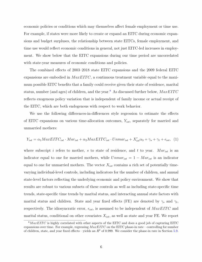
Parents spend considerable sums investing in their children’s development, with their own time among the most important forms of investment. Given well-documented effects of the Earned Income Tax Credit (EITC) on maternal labor supply, it is natural to ask how the EITC affects other time allocation decisions, especially time with children. We use the American Time Use Surveys to study the effects of EITC expansions since 2003 on time devoted to a broad array of activities, with considerable attention to the amount and nature of time spent with children. Our results confirm prior evidence that the EITC increases maternal work and reduces time devoted to home production and leisure. More novel, we show that the EITC also reduces time spent with children; however, almost none of the reduction comes from time devoted to “investment” activities. Effects are concentrated among socioeconomically disadvantaged mothers, especially those that are unmarried. Results are also most apparent for mothers of young children. Altogether, our results suggest that the increased work associated with EITC expansions over time has done little to reduce the time mothers devote to active learning and development activities with their children.

JEL Classification Codes: D13, H24, H31, H53, I31, I38, J13, J22

Key Words: EITC, tax policy, time use, child investment, female labor supply

Acknowledgments: We would like to thank Elira Kuka, Brenden Timpe, and Riley Wilson for comments and Gabe Goodspeed and Qian Liu for excellent research assistance. This research was funded by the Smith Richardson Foundation and the Upjohn Institute.

1. Introduction

A growing literature documents the importance of family investments for child develop-

ment (e.g., see surveys by Cunha et al., 2006; Heckman and Mosso, 2014; Kalil, 2015), with

parental time becoming an increasingly important form of investment (e.g., Lee and Bowen,

2006; Del Boca et al., 2014; Carneiro et al., 2015; Caucutt et al., 2020). Caucutt et al. (2020)

document that more than two-thirds of all family expenditures on child development (for

children ages 12 or younger) come in the form of parental time investments.

It is tempting to assume that the more time mothers spend working, the less they must

spend with their children. Yet, such an assumption is clearly at odds with the time series

for female labor supply and time with children, which have both increased substantially

in recent decades.1 Cross-sectional relationships are also at odds with a direct trade-off.

For example, Guryan et al. (2008) show that more-educated parents both work more and

spend more time with their children compared to less-educated parents. Clearly, parents

devote time to many leisure and home production activities besides child care (Becker, 1965;

Kooreman and Kapteyn, 1987; Aguiar and Hurst, 2007), and these activities trade off with

work.

Understanding parental (especially maternal) time allocation decisions is critical for un-

derstanding the impacts of tax and transfer policies, including many welfare-to-work initia-

tives, on investments in children and child development. The Earned Income Tax Credit

(EITC), the focus of our study, is one of the most significant tax/transfer policies in the

United States, impacting millions of low- to middle-income families. Dahl and Lochner

(2012, 2017), Chetty et al. (2011), Bastian and Michelmore (2018), Manoli and Turner

(2018) and Agostinelli and Sorrenti (2018) estimate positive impacts of expansions in the

EITC on test scores, educational attainment, employment, and earnings of economically dis-

advantaged children.2 These studies emphasize the increase in financial resources for families1See, e.g., Bryant and Zick (1996), Gauthier et al. (2004), Sayer et al. (2004), Bianchi and Robinson

(1997), Craig (2006), Kimmel and Connelly (2007), Guryan et al. (2008), and Kalil et al. (2012) for evidenceon growing parental time with children, while Costa (2000), Goldin (2006), Fernández (2013), and Bastian(2020) document the substantial increase in female labor supply over time.

2Hoynes et al. (2015), Averett and Wang (2018), and Braga et al. (2019) show that the EITC also improveschildren’s health.

1

that benefit from EITC expansions, with much of the increase in family income coming from

greater labor force participation and higher pre-tax family earnings.3 However, Agostinelli

and Sorrenti (2018) and Bastian and Michelmore (2018) also examine concerns that the addi-

tional time mothers spend working could offset the benefits associated with greater financial

resources. Indeed, several studies estimate negative effects of full-time maternal employment

on child development (Brooks-Gunn et al., 2002; Ruhm, 2004; Bernal, 2008).4

Even if the EITC increases maternal labor supply by increasing net-of-tax wages for

low-income families, it need not reduce parental time investments in children. The positive

income effects from higher wages can create incentives to increase overall investments in

children. As shown by Caucutt et al. (2020), if all investment inputs are sufficiently comple-

mentary, families may wish to increase all types of investments, including time investments,

despite the increase in their opportunity costs. Thus, higher wages may cause parents to

substitute leisure and home production for time at work with little, or even positive, effects

on time spent with children. Indeed, Kooreman and Kapteyn (1987) and Kimmel and Con-

nelly (2007) estimate that increases in maternal wages lead to reductions in time devoted to

leisure and home production but much weaker or even modest positive effects on child care.

Looking more directly at impacts of the EITC, studies spanning three decades of re-

search have consistently concluded that it raises employment among single mothers (Hoffman

and Seidman, 1990; Eissa and Liebman, 1996; Meyer and Rosenbaum, 2001; Grogger, 2003;

Hoynes and Patel, 2018; Bastian, 2020).5 Much less is known about changes in other uses

of time. Looking at a broader set of tax policies, Gelber and Mitchell (2012) estimate that

policies that encourage maternal labor supply also reduce time spent on home production.

In their analysis of the EITC using data from the Panel Study of Income Dynamics, Bas-

tian and Michelmore (2018) estimate modest and statistically insignificant effects of EITC

expansions on the time parents spend with their children; however, their sample size is small

and estimates imprecise.3For these mothers, the EITC also improves health (Evans and Garthwaite, 2014), reduces stress and

financial insecurity (Mendenhall et al., 2012; Jones and Michelmore, 2016), and reduces poverty (Hoynes andPatel, 2018).

4Using family and child fixed effects approaches, Heiland et al. (2017) estimate that mothers who work10 hours more per week spend about 3-4 percent less time with their children.

5Recently, Kleven (2019) has challenged this conclusion.

2

In this paper, we use the 2003-2018 American Time Use Surveys (ATUS) to study, in

detail, the time allocation responses of mothers to state and federal expansions in the EITC

with an emphasis on time spent with children. More specifically, our main (differences-in-

differences style) approach estimates the effects of changes in the maximum EITC benefit

level on time spent in different activities, accounting for basic family demographic char-

acteristics, state and time fixed effects (both interacted with marital status and mothers’

educational attainment), and time-varying state-specific measures of economic conditions

and welfare/tax policies. Because ATUS contains detailed information on respondent activ-

ities and who they were with during each activity, we are able to estimate the same basic

specifications for a variety of time allocation activities, with and without children.

We begin by estimating impacts of the EITC on mothers’ labor supply over the 2003–

2018 period, noting that most previous research examines earlier expansions (especially the

major expansion from 1993 to 1996). There is some disagreement on the impacts of EITC

expansions after the mid-1990s, with Bastian and Michelmore (2018) and Bastian and Jones

(2019) estimating moderate positive effects (consistent with the previous literature) and

Kleven (2019) finding more modest effects of the 2009 federal expansion and no effects of

state expansions. Our approach is more similar to that taken by Bastian and Michelmore

(2018) and Bastian and Jones (2019),6 reaching similar conclusions: expansions of the EITC

since 2003 have led to increased labor force participation, time spent working, and earnings

among unmarried mothers. We also find suggestive evidence that federal EITC expansions

had larger effects on labor supply—and on other categories of time use—than state EITC

expansions. This result could reflect differences in public awareness of smaller state vs. larger

federal expansions, a general issue highlighted in Chetty et al. (2013).

Next, we show that the increased time working comes at the expense of both leisure

and home production activities. Decomposing single mothers’ time use into time with and

without children, we estimate reductions in home production and leisure time with children,

but no decrease in these activities without children.

Finally, we closely examine how time with children changes, exploring impacts on “in-6Kleven (2019) takes an event-study approach that does not leverage differences in the magnitude of

different expansions for identification.

3

vestment” (e.g., reading, playing, helping with homework, providing medical care) vs. “non-

investment” activities. Our estimates suggest no effect of the EITC on total investment time

for families with children of all ages. Reductions in time with children are almost exclusively

observed for passive non-investment activities like mothers’ own personal care, housework,

and errands. One interesting exception is that both married and unmarried mothers respond

to EITC expansions by spending less time providing or obtaining medical care for their chil-

dren, which may be due to general improvements in children’s health as estimated by Hoynes

et al. (2015), Averett and Wang (2018), and Braga et al. (2019). We also observe modest

increases in the time both single and married mothers play with their children, consistent

with increases in family income if play time is a luxury for parents.

2. Federal and State EITC Policy Details

The EITC distributes over $65 billion a year to almost 30 million low-income families,

lifting 6 million people out of poverty (Center on Budget and Policy Priorities, 2019). Total

EITC benefits are determined by annual earnings, number of children, state of residence,

and marital status. Figure 1 shows the relationship between EITC benefits and household

earnings by the number of children and marital status for 2018. As is clear from the figure,

the EITC contains a phase-in region, where benefits increase with earnings; a plateau region,

where benefits do not change with earnings; and a phase-out region, where benefits decrease

with earnings. Households that earn beyond this phase-out region are not eligible for the

EITC. In 2018, federal EITC benefits were worth over $6,000 for households with 3 or

more children earning between about $14,000 and $24,000. Maximum possible benefits

available to households with 0, 1, and 2 children were approximately $500, $3,500, and

$5,500, respectively.

Figure 2 shows the evolution of maximum benefits by number of children over time.

The largest EITC expansion occurred between 1993 and 1996, which increased benefits

dramatically for those with at least 2 children. Our analysis covers the years 2003–2018.

The only change in the federal EITC schedule during this period occurred in 2009, when the

maximum credit available to families with 3 or more children increased by about $1,000.

4

As of 2018, 29 states had their own EITC as well. State EITC benefits generally “top-up”

federal EITC benefits by a fixed percent, varying from about 3 to 40 percent (for values up

to $220 to $2,800). Combined, the federal and state EITC can amount to over $9,000 per

year, with the average recipient receiving over $2,500 a year. Figure 3 shows a map of state

EITC rates (as a fraction of federal benefits) in 2000, 2005, 2010, and 2017. Figure A.1

shows the maximum possible federal plus state EITC benefits over time: there is substantial

variation in EITC policy across states within each year.

We combine state and federal annual maximum EITC benefit amounts (based on state of

residence, marital status, number and ages of children by year) into the variable,MaxEITC,

which we measure in thousands of real 2018 dollars.7 Panel A in Figure 4 shows the dis-

tribution of MaxEITC for women with 0, 1, 2, and 3 or more children based on our main

sample of women ages 18–49 in the 2003–2018 ATUS. Panel B in Figure 4 shows the dis-

tribution of MaxEITC before and after the 2009 federal EITC expansion. Together, these

figures illustrate the type of EITC variation over time and across states that we exploit for

identification.

EITC-eligible children must be age 18 or younger, age 19–23 and a full-time student, or

any age and disabled. However, incorporating these older children could introduce endogene-

ity and we avoid this concern by defining EITC-eligible dependents as age 18 or younger.

3. Empirical Strategy

Although the largest EITC expansion occurred in the 1990s, our time-use data only goes

back to 2003. Fortunately, during our sample period, there is substantial identifying variation

across states and years generated by state EITC policy changes and the 2009 federal EITC

expansion, as well as variation within states and years generated by the large difference in

EITC benefits by number of children (see Figures 3 and 4). EITC policy variation allows us

to compare outcomes for women within states and across years, as well as across states and

within years.

An identifying assumption is that EITC policy expansions are not correlated with other7We use the Consumer Price Index for all Urban Consumers to adjust for inflation.

5

economic policies or conditions which may themselves affect female employment or time use.

For example, if states were more likely to create or expand an EITC during economic expan-

sions and budget surpluses, the relationship between state EITCs, female employment, and

time use would reflect economic conditions in general, not just EITC-led increases in employ-

ment. We show below that the EITC expansions during our time period are uncorrelated

with state-year measures of economic conditions and policies.

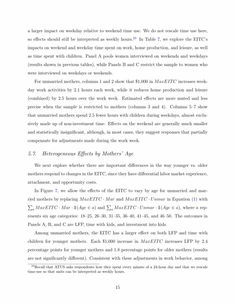
The combined effects of 2003–2018 state EITC expansions and the 2009 federal EITC

expansions are embodied in MaxEITC, a continuous treatment variable equal to the maxi-

mum possible EITC benefits that a family could receive given their state of residence, marital

status, number (and ages) of children, and the year.8 As discussed further below,MaxEITC

reflects exogenous policy variation that is independent of family income or actual receipt of

the EITC, which are both endogenous with respect to work behavior.

We use the following differences-in-differences style regression to estimate the effects

of EITC expansions on various time-allocation outcomes, Yist, separately for married and

unmarried mothers:

Yist = α1MaxEITCist ·Marist + α2MaxEITCist · Unmarist +X ′istα3 + γs + γt + εist, (1)

where subscript i refers to mother, s to state of residence, and t to year. Marist is an

indicator equal to one for married mothers, while Unmarist = 1 −Marist is an indicator

equal to one for unmarried mothers. The vector Xist contains a rich set of potentially time-

varying individual-level controls, including indicators for the number of children, and annual

state-level factors reflecting the underlying economic and policy environment. We show that

results are robust to various subsets of these controls as well as including state-specific time

trends, state-specific time trends by marital status, and interacting annual state factors with

marital status and children. State and year fixed effects (FE) are denoted by γs and γt,

respectively. The idiosyncratic error, εist, is assumed to be independent of MaxEITC and

marital status, conditional on other covariates Xist, as well as state and year FE. We report8MaxEITC is highly correlated with other aspects of the EITC and does a good job of capturing EITC

expansions over time. For example, regressingMaxEITC on the EITC phase-in rate—controlling for numberof children, state, and year fixed effects—yields an R2 of 0.999. We consider the phase-in rate in Section 5.9.

6

standard errors that are robust to heteroskedasticity and clustered at the state level.9 ATUS

weights are used in all specifications.

We also explore whether the effects vary by other family characteristics conditional on

marital status, estimating equations of the form

Yist =MaxEITCist·Marist·Z ′istβ1+MaxEITCist·Unmarist·Z ′

istβ2+X′istβ3+γs+γt+εist, (2)

where Zist reflects a vector of indicator variables for mothers’ race, educational attainment,

or predicted probability of low income (as described below).

4. Data from the American Time Use Surveys

We use the 2003–2018 Bureau of Labor Statistics’ American Time Use Survey Data

(ATUS). ATUS is the “nation’s first federally administered, continuous survey on time use in

the United States. The goal of the survey is to measure how people divide their time among

life’s activities” (U.S. Bureau of Labor Statistics, 2019).10 ATUS data are linked to the

Current Population Survey (CPS) and contain rich demographic and geographic information.

We keep all women ages 18–49 in the main sample, 58,090 observations. Of these women,

43,685 are mothers and 14,940 are unmarried mothers.

With the use of time diaries, ATUS asks respondents how they spent every minute of a 24-

hour day, also recording with whom they spent their time. We scale reported time use so that

units can be interpreted as weekly hours. We divide time use into three broad categories: paid

work activities (including work, commuting, job search, and job-related socializing); home

production; and leisure.11 All time unaccounted for by these categories can be classified as

schooling, sleep, and “uncategorized.”12 We also determine whether time in each activity was

spent with children, creating our measure of “time with children.” Additionally, we create9Alternate clustering and standard error specifications yield similar results, as does restricting the sample

to unmarried mothers (available upon request).10Time-use data exists for earlier years, but these samples are relatively small (generally 2,000–4,000

observations per year, compared to 10,000–20,000 per year for 2003–2018) and contain fewer covariates.11Home production includes cooking and meal preparation, housework, car maintenance, taking care of

garden or pets, travel related to household activities, other household management, taking care of childrenor other household members, and shopping. Leisure time includes exercise and sports, games, watching TVor movies, computer activity, socializing, talking on the phone or communicating, reading, listening to musicor the radio, arts and entertainment, hobbies educational activities, and own medical care.

12The mean value of uncategorized time is only 1.36 hours, out of 168 weekly hours.

7

a measure of “investment” time, a subset of leisure and home production activities in which

the mother was with her child. Investment time includes activities like doing homework

and children’s education, providing and obtaining medical care, playing games or sports,

doing crafts, or attending museums or events together. See the Data Appendix for complete

details.

To measure labor supply, we have a few options available, some based on ATUS time-

diary data and others based on linked CPS data. Our preferred measures are labor force

participation (LFP, an indicator equal to one if employed or unemployed) and hours worked

last week, both from CPS survey data. We use these CPS-based measures unless otherwise

specified; however, results are qualitatively similar across measures.13

For time-use activities not specifically related to time with children (e.g., working, home

production, leisure), we often study the full sample of women, since the largest incentive

differences from EITC changes are between women with and without children. Between

these two groups, the EITC’s effect on labor supply and time-use will be most detectable.

For outcomes related to spending time with children, we focus exclusively on mothers with

children in the household.

Table 1 reports summary statistics for all women, all mothers, and unmarried women ages

18–49 (using ATUS weights). On average, women have 1.2 children, are 33.8 years old, 52

percent are married, 89 and 33 percent finished high school and college, 13 and 17 percent are

black or Hispanic, and have $26,000 and $66,000 in individual and total household earnings.

Average MaxEITC is $3,337, while the average EITC benefits women are actually eligible

for is $668, with 24 percent receiving some benefits.14 Compared to the sample of all women,

mothers are on average older, are more likely to be married, have lower education, are more

likely to be nonwhite, are less likely to be employed, and have lower individual earnings

but similar levels of household earnings. Compared to all mothers, unmarried mothers are

on average more socially and economically disadvantaged: younger with lower education,13As already discussed, ATUS also asks about time spent on work activities, but this measure is noisier,

since it is based on a 24-hour period, which may occur on a weekend day. Other available measures of laborsupply in the CPS include employed and usual weekly work hours.

14EITC benefits imputed from NBER’s TAXSIM (Feenberg and Coutts, 1993). Details here: https://www.nber.org/taxsim/.

8

more likely to be nonwhite, eligible for more EITC benefits ($1,525 vs. $1,079), and more

likely to be eligible for at least some benefits (51 vs. 35 percent). We also report summary

statistics for the state-year variables we control for in our analysis (discussed in Section 5.1):

state GDP growth rate, state per capita GDP, state unemployment rate, minimum wage,

maximum welfare benefits for a family with 1, 2, 3, or 4 children.

Table 2 uses the sample of mothers and reports summary statistics for time-use variables.

Among all mothers, average weekly hours (from CPS) are 21.6 for work, 46.5 for home

production, 33.4 for leisure, 38.7 for time with children, and 6.0 for investment into children.

Table 2 also shows that mothers with more children spend less time on work and leisure,

while they spend more time on home production, with children, and investing in children.15

Figure 5 shows how weekly hours spent working, with children, and investing in children

vary with children’s ages. On average, mothers with infants work 15 hours per week, and

work hours steadily increase with a child’s age, reaching 20 hours by age 6 and 25 hours by

age 17. By contrast, maternal time with children monotonically decreases with a child’s age:

mothers spend about 60 hours per week with infants, falling to 40 hours by age 8 and 20

hours at age 17. We also observe a steady decline in investment time as children age, falling

from about 10 hours per week for infants to 8 hours per week at age 4, to 2 hours per week

at age 17. Figure 5 also displays the 25th and 75th percentiles for hours with children and

investing in children by age of child.

5. Results

In this section, we first establish the exogeneity of state EITC changes. We then examine

effects of the EITC on maternal labor supply before turning to impacts on other uses of

time, including home production, leisure, and time with children. We decompose time with

children into “investment” and “non-investment” activities to better understand how changes

in the EITC might impact child development via time-use decisions. We also study whether

time-use effects of the EITC differ on weekdays vs. weekends, and whether there are differ-15In the Online Appendix, we also show the full distribution for each category of time use by number

of children. Appendix Figures A.2, A.3, and A.4 show the distribution of hours worked last week (CPSmeasure), home production, and leisure. Appendix Figures A.5 and A.6 show the distribution of total hourswith children and investment hours in children.

9

ential effects based on age of the mother or on the ages of children in the household. Finally,

we explore the robustness of our estimates to different sets of controls and specifications that

leverage variation from state vs. federal EITC expansions.

5.1. Exogeneity of State EITCs

To examine whether EITC policy expansions are correlated with other state policies or

economic conditions, we regress measures of state EITCs on several state-year characteristics,

including GDP, unemployment rate, the top marginal income tax rate, the minimum wage,

welfare generosity for families with 1, 2, or 3 or more children, and sales tax rates. We also

include lags of each of these variables along with state and year FE.

In Table 3, we find that across four specifications and dozens of variables, only two

estimates are significant at the 10 percent level. The four specifications are combinations of

using the sample of all states or states that ever had a state EITC, and of using maximum

state EITC benefits or the state EITC rate as outcomes. Testing for the joint significance

of these state-level traits yields p-values between 0.85 and 0.95.16 Although we find little

evidence that these traits are associated with state EITCs, we control for these state-level

traits throughout our analysis.

5.2. Labor Supply

We begin our analysis of time allocation decisions by studying the impact of the EITC

on labor supply, earnings, and family resources.

Among all women, Table 4 Panel A shows that a $1,000 increase in MaxEITC increases

average labor force participation (1.7 percentage points), weekly work hours (0.74), earnings

($1,166), and EITC benefits ($245). Here, work hours refers to hours worked last week, as

reported in CPS data. By marital status, Table 4 Panel B shows larger estimated effects

among unmarried women on LFP (3 percentage points), weekly work hours (1.2), earnings

($1,597), EITC benefits ($301), and the probability of being eligible for any EITC benefits

(1.9 percentage points). Among married women, we find insignificant effects, except on16Contrary to these results, there is some evidence that state economic conditions or policies were associ-

ated with state EITC expansions in the 1990s (e.g., Hoynes and Patel (2018)).

10

EITC benefits ($188).17 These differences by marital status are all statistically significant

(p-values < 0.001) and are largely consistent with previous evidence on how the EITC affects

unmarried and married mothers (Eissa and Hoynes, 2006; Bastian and Jones, 2019).18

Restricting the sample to mothers, estimates in Table 4 Panel C are very similar to

(though less precise than) estimates in Panel B based on all women. For unmarried moth-

ers, each $1,000 increase in MaxEITC raises LFP (2.4 percentage points), hours worked

last week (0.83), earnings ($1,222), and EITC benefits ($361). For married mothers, re-

sults are all insignificant, except for EITC benefits ($238). Appendix Table A.1, presents

a similar pattern of results for subgroups of mothers by marital status interacted with race

or educational attainment (based on estimating equation (2)). Impacts are generally larger

and often significant for unmarried mothers, regardless of race and education, while impacts

are mostly small and statistically insignificant for all types of married mothers (except for

positive effects on EITC benefits).

The labor supply results presented thus far are based on CPS data on LFP and hours

worked last week. Appendix Table A.2 shows that results are robust to studying other

measures of labor supply from the CPS (usual weekly work hours, employed, and non-

self-employed LFP) or from time diary data from ATUS (weekly work hours, working > 0

hours/week, working ≥ 20 hours/week, and working ≥ 40 hours/week).

In Appendix Table A.3 we isolate the effects of state EITC expansions by limiting the

sample to years before or after the 2009 federal EITC expansion. In these specifications,

variation in MaxEITC comes exclusively from state EITC expansions. We find that both

before and after 2009, EITC expansions are associated with increases in LFP and weekly

hours worked among unmarried mothers, while effects for married mothers are much weaker

and mostly insignificant. These results also highlight that our estimates are not driven by

changes in labor supply associated with the Great Recession.17Increases in EITC benefits are due to a mechanical and behavioral component. Even with no change in

labor supply, increases in MaxEITC will lead to increased EITC benefits by those already receiving it.18Our study implictly addresses Kleven (2019) and his claim that the EITC does not impact labor supply

in two main ways: one, we focus on 2003–2018, well after welfare reform, ensuring that our EITC estimatesare not confounded with the simultaneity of 1990s EITC expansions and welfare reform; and two, by usingtime-use outcomes, we provide an alternate approach to testing whether the EITC impacted mothers.

11

5.3. Effects on Broad Categories of Time Allocation

Based on the labor supply results in Table 4, we expect to find that the EITC led to

reductions in the amount of time unmarried mothers spend on non-work activities and that

the EITC had little effect on the time-use of married mothers. In Table 5, we divide each

woman’s 168 weekly hours into home production, leisure, work activities, school, sleep, and

“uncategorized” using the ATUS time diary activity data.

For unmarried women, Panel A shows that $1,000 inMaxEITC reduces home production

and leisure (1.04 and 0.74 hours), increases work activities (1.50 hours), and has little effect

on school, sleep, and uncategorized time. For married mothers, whose labor supply is largely

unaffected by the EITC, we see insignificant effects on other uses of time as well.

Panel B reveals similar patterns for the sample of mothers; however, estimated effects

on work activities are muted for unmarried mothers relative to all unmarried women. Con-

sequently, we also estimate more muted impacts on their other uses of time. Among single

mothers, a $1,000 increase in MaxEITC increases work activities by 0.63 hours per week

and reduces home production by 0.91 hours per week and leisure by 0.40 hours per week.

For married mothers, all impacts are statistically and economically insignificant.

5.4. Time with Children and Parental Time Investment in Children

We now look specifically at how mothers spend their time with children. Table 5 Panel

B decomposes home production and leisure into time with and without children.19 Among

unmarried mothers, each $1,000 in MaxEITC reduces home production and leisure time

with children (−1.17 and −0.53 hours per week) but has small and insignificant effects on

home production and leisure time without children (0.26 and 0.12 hours per week).

Tables A.6 and A.7 decompose the reduction in home production and leisure time with

children (for unmarried mothers) into eight subcategories. Table A.6 shows that $1,000 in

MaxEITC leads to statistically significant reductions in personal care (0.11 hours), house-

work (0.23 hours), and traveling/errands (0.19 hours). Reductions in waiting and shopping19Time with children is not a mutually exclusive category, but rather overlaps with the other categories

shown in Table 5. We do not decompose work, school, sleep, or uncategorized time into with/withoutchildren, because time with children is negligible for these activities and pre-2010 ATUS did not collect “withwho” information when respondents reported sleeping, grooming, personal/private activities, or working.

12

(0.19 hours) are also substantial, though statistically insignificant. (We estimate negligible

effects on all remaining home production subcategories.) Table A.7 shows that the entire

reduction in leisure time with children comes from time spent socializing and relaxing.

Since the EITC reduces time that mothers spend with their children, it is natural to worry

about impacts for parental time investments (e.g., reading together, help with homework,

playing, doctor visits) and child development. Of course, reductions in time mothers spend

with children may not have much of an effect on child development if this time would have

been spent watching television, cleaning the house, etc. To investigate this issue, Table 6

decomposes maternal time spent with children into investment and non-investment activities.

Each $1,000 in MaxEITC reduces total time unmarried mothers spend with children by

1.61 hours per week, but this decrease is explained completely by non-investment time, which

declines by 1.56 hours per week. This reduction in non-investment time with children comes

more out of home production time (0.9 hours per week) than leisure (0.75 hours per week),

but reductions in both are significant.

Although changes in total time spent on investment are negligible, this does not necessar-

ily mean that mothers do not adjust their time across different types of investment activities.

Given the changes in family income induced by EITC expansions, parents may adjust the

types of investment activities they engage in depending on the income elasticities of the

activities. These elasticities may differ, for example, because of different complementarities

with purchased goods and services or due to heterogeneous parental preferences for different

types of activities (e.g., parents may enjoy some activities more than others).

We consider the impacts of EITC expansions on the investment subcategories of aca-

demic, health, and “other” investment time. Table 6 shows very small and insignificant

effects of MaxEITC on academic investment time, modest but statistically significant re-

ductions in health investment time, and offsetting (but mostly insignificant) increases in

“other” investment time. Appendix Table A.8 shows that the reductions in health invest-

ment reflect less time spent providing and obtaining medical care for children. This may

reflect improvements in health that have previously been attributed to the EITC (Hoynes

et al., 2015; Averett and Wang, 2018; Braga et al., 2019) such that children require less

13

medical attention.20 Appendix Table A.8 also shows that increases in “other” investment

time are entirely explained by increases in time spent playing (0.24 and 0.16 hours per week

for unmarried and married mothers, respectively). The sizeable impacts on play time for

married mothers suggests that these responses may be due to the increased family income

associated with EITC expansions. This might be expected if parents view time spent playing

with children as a luxury.21

5.5. EITC Effects on the Distribution of Time Use

We now briefly consider the impacts of EITC expansions on the distributions of weekly

hours of work, home production, leisure, time with children, and time investing in children.

Specifically, we estimate the effects of the EITC on the probability that unmarried mothers

spend more than x hours per week on an activity using the following specification:

1(Yist > x) = δ1MaxEITCist ·Marist+δ2MaxEITCist ·Unmarist+X ′istδ3+γs+γt+εist. (3)

In Figure 6, we restrict the sample to mothers. Panels A–D show that an increase in

MaxEITC raises the probability of working up to—but not above—40 hours per week.

Thus, the EITC draws women into the labor market but does not increase work beyond full

time. An increase in MaxEITC significantly reduces home production time in the 50–90

hours per week range, while it only reduces leisure time at the low end of the distribution

(10–20 hours per week). The EITC reduces time spent with children throughout much of

the distribution; however, investment time decreases most for the 1–30 hours range, while

effects are negligible for mothers who spend more than 40 hours per week on investment.22

5.6. Weekends vs. Weekdays

Because the EITC increases work among unmarried mothers, these mothers must reallo-

cate the rest of their time accordingly. Since most jobs are Monday to Friday, we may expect20For example, increases in family income or employment may lead to improvements in health insurance.21Indeed, Krueger et al. (2009) find that parents enjoy time spent playing with their children relative to

nearly any other activity they study. The larger increase in time spent playing for married mothers is alsoconsistent with modest negative impacts of the EITC on their labor supply. While we do not find a negativeeffect on the average labor supply of married mothers, we do find a decrease among younger married mothersin Section 5.7, lining up with previous studies (Eissa and Hoynes, 2004; Bastian and Jones, 2019).

22Appendix Figure A.7 shows very similar effects on the distribution of hours of work, home production,and leisure for the sample of all women.

14

a larger impact on weekday relative to weekend time use. We do not rescale time use here,

so effects should still be interpreted as weekly hours.23 In Table 7, we explore the EITC’s

impacts on weekend and weekday time spent on work, home production, and leisure, as well

as time spent with children. Panel A pools women interviewed on weekends and weekdays

(results shown in previous tables), while Panels B and C restrict the sample to women who

were interviewed on weekdays or weekends.

For unmarried mothers, columns 1 and 2 show that $1,000 inMaxEITC increases week-

day work activities by 2.1 hours each week, while it reduces home production and leisure

(combined) by 2.5 hours over the work week. Estimated effects are more muted and less

precise when the sample is restricted to mothers (columns 3 and 4). Columns 5–7 show

that unmarried mothers spend 2.5 fewer hours with children during weekdays, almost exclu-

sively made up of non-investment time. Effects on the weekend are generally much smaller

and statistically insignificant, although, in most cases, they suggest responses that partially

compensate for adjustments made during the work week.

5.7. Heterogeneous Effects by Mothers’ Age

We next explore whether there are important differences in the way younger vs. older

mothers respond to changes in the EITC, since they have differential labor market experience,

attachment, and opportunity costs.

In Figure 7, we allow the effects of the EITC to vary by age for unmarried and mar-

ried mothers by replacing MaxEITC ·Mar and MaxEITC · Unmar in Equation (1) with∑aMaxEITC ·Mar · 1(Age ∈ a) and

∑aMaxEITC · Unmar · 1(Age ∈ a), where a rep-

resents six age categories: 18–25, 26–30, 31–35, 36–40, 41–45, and 46–50. The outcomes in

Panels A, B, and C are LFP, time with kids, and investment into kids.

Among unmarried mothers, the EITC has a larger effect on both LFP and time with

children for younger mothers. Each $1,000 increase in MaxEITC increases LFP by 2.4

percentage points for younger mothers and 1.8 percentage points for older mothers (results

are not significantly different). Consistent with these adjustments in work behavior, among23Recall that ATUS asks respondents how they spent every minute of a 24-hour day and that we rescale

time-use so that units can be interpreted as weekly hours.

15

younger mothers we observe reductions of over two hours per week spent with children and

insignificant effects on child investment. Among older mothers, effects on time with children

are smaller and close to zero for mothers over age 40. While statistically insignificant, we

find a small increase in investment among older mothers, consistent with positive income

effects and no offsetting reduction in their non-work time budget.

The effects for married mothers reveals an interesting pattern: for young married mothers

under age 25, the EITC has a negative effect on LFP and a positive effect on time with—

and investment into—children; while the EITC has a marginally significant effect on those

aged 26-30 and null effects on those over age 30. The effects on younger married mothers

are consistent with previous research finding small negative effects on the labor supply of

married mothers (Eissa and Hoynes, 2004; Bastian and Jones, 2019).

5.8. Heterogeneous Effects by Children’s Age

Since mothers typically spend progressively more time working and less time with children

as their children grow older (see Figure 5), we next explore whether responses to EITC

expansions depend on children’s ages. To do so, we consider the effects of total time spent

with children in age group a (i.e., ages 0–2, 3–5,..., 18–20, 21–22), Y aist, by estimating separate

regressions for different age groups as follows:

Y aist = φa

1MaxEITCist ·Marist + φa2MaxEITCist · Unmarist +X ′

istφa3 + γas + γat + εaist. (4)

Here, φa1 and φa

2 reflect the impact of a $1,000 increase in the maximum EITC benefit on

hours with (or investing in) children who are in age group a for married and unmarried

mothers, respectively. By definition, these effects reflect impacts for mothers with at least

one child in age group a.24 Most children older than 18 are not EITC-eligible, unless they are

full-time students or disabled. However, we consider children up through age 22 as quasi-

placebo tests, since any effects for these (mostly ineligible) children would likely indicate

spurious effects of unmeasured factors.

Figure 8 reports the effects of MaxEITC on time spent with and investing in children

of each age. A $1,000 increase in the maximum EITC benefit significantly increases mar-24Each regression uses the full sample of mothers with Y a

ist = 0 for mothers with no children in age groupa. Xist contains the full set of controls.

16

ried mothers’ time spent with and investing in children ages 3–11: time spent with these

young children increases by 0.6–1.3 hours per week (Panel A), while time spent investing

increases by about one-third of an hour (Panel B). The same increase in MaxEITC signifi-

cantly reduces the time unmarried mothers spend with children ages 6–14 by about an hour

(Panel A); however, it has no significant effects on their investment time with children of

any age (Panel B). Finally, we note that effects on time spent with (or investing in) children

ages 21–22 are both negligible and insignificant, consistent with their ineligibility for EITC

(in most cases).

5.9. Robustness

In this section, we examine whether our results are robust to alternate sets of controls,

alternate measures of the EITC, and whether mothers with the highest predicted probability

of having low income are most affected by EITC policy changes.25

Alternate Controls: In Tables 8 and 9, we test whether our main results are robust

to various sets of controls. Columns 1–3 progressively add year, state, and number of kids

FE; demographic traits; whether the time-use data was collected on a weekend or weekday;

and measured state-year factors (e.g., unemployment rate, minimum wage). Column 3 is

the full set of controls used for all results above. Columns 4–6 examine whether the results

are robust to progressively adding controls for state-specific time trends, state-specific time

trends interacted with an indicator for unmarried, and state-year factors interacted with

indicators for unmarried and having any children. These controls account for general trends

in unobserved state-specific factors by marital status and allow for measured state policies

and economic conditions to differentially affect time allocation decisions by marital status

and children in the household. Finally, column 7 adds state × year FE, which largely

absorbs variation in state EITC expansions and identifies the impact of the 2009 federal

EITC expansion, while column 8 adds year × number of children FE, largely absorbing

variation in the federal expansion (and other nationwide trends that differentially affect

families of different sizes), identifying the impact of state EITC expansions.

Table 8 uses the sample of all women and examines the following outcomes: LFP, weekly25When we separately estimate effects of the EITC by month, we find similar results across months.

17

work hours, and home production plus leisure hours. Across controls, the estimated effect

on LFP for unmarried women ranges from 3.0 to 3.9 percentage points; estimated effect on

weekly work hours ranges from 0.9 to 1.6; and the effect on home production and leisure

ranges from −1.6 to −2.2 hours. Among married mothers, all specifications show consistent

evidence that the EITC has little impact on labor supply, while there is a modest reduction

in home production and leisure time.

Table 9 uses the sample of mothers and examines the same three outcomes from Table 8,

as well as time with children and time investing in children. Results for the first three out-

comes are similar to but more muted and less precise than those in Table 8. For unmarried

mothers, the estimated effects on time with children range from −1.2 to −2.2 hours per

week across all specifications, while estimated effects on time investing in children are con-

sistently very small and statistically insignificant. Among married mothers, all estimates are

insignificant.

Comparing columns 7 and 8 in both Tables 8 and 9 suggests that the 2009 federal EITC

expansion had larger effects on labor supply, home production and leisure, and time with

children than did state EITC expansions (for unmarried mothers).

Alternate Measures of the EITC: Table A.5 shows that results are robust to alternate

measures of EITC expansions, specifically the EITC phase-in rate.26 We find consistent

evidence that EITC expansions lead to increases in LFP and work hours, coupled with

reductions in home production and leisure time, for unmarried women and mothers. The

expansions also cause unmarried mothers to reduce their total time with children but have

little impact on their investment time with children. Among married women and mothers,

our estimates suggest no effect of changes in EITC phase-in rates on their time allocation.

Subgroups Based on Predicted Household Income: We have shown how the

EITC’s impact varies by marital status, race, and education. In general, more economi-

cally disadvantaged mothers (e.g., unmarried, nonwhite, less educated) are more responsive

to changes in the EITC. To better examine the role of economic disadvantage, we now take26Notice that if the federal phase in rate is 40 percent and the state EITC matches 20 percent of the

federal EITC, then the total phase-in rate is 0.40(1+0.20)=0.48. MaxEITC and phase-in rate are highlycorrelated; see footnote 8.

18

into account several (exogenous) demographic factors to predict which mothers are most

likely to have low household income (i.e., income less than $20,000 in 2017 dollars).27 These

women are most likely to find themselves on the phase-in or plateau regions of the EITC

schedule, encouraging their labor supply. Dividing mothers into terciles based on their pre-

dicted probability of low income, we estimate Equation (2) using these predicted probability

terciles as Zist variables interacted with MaxEITC and marital status. (Results are simi-

lar if we estimate a specification that only interacts the predicted probability terciles with

MaxEITC, estimating an average effect across married and unmarried mothers.)28

Table 10 shows consistent evidence that mothers with the highest predicted probability

of having low household income are most affected by changes in the EITC. For unmarried

mothers, we estimate positive effects on LFP and negative effects on time with children and

time spent in home production or leisure for each tercile, with consistently larger effects for

mothers that are more likely to be economically disadvantaged. Among unmarried mothers

that are most likely to have low household income, each $1,000 increase in maximum EITC

benefits raises LFP by 3 percentage points, while it lowers home production and leisure

combined by 2.0 hours per week and reduces time with children by 2.1 hours per week.

Importantly, none of our subgroups of unmarried mothers respond by reducing investment

time with their children (results are negative, but small and insignificant).

Among married mothers, we find little evidence of any effects, except for a modest increase

in investment time with children among those least likely to be of low income. Altogether,

these results suggest that marital status is important even when conditioning on predicted

household income.27Specifically, we use OLS to estimate the probability that mothers have household income less than

$20,000 (in 2017 dollars) controlling for number of children FE, four categories of mothers’ educationalattainment (<12, =12, 13–15, and >16), race, age, and birth year, as well as year and state FE. While wedo not use marital status to predict low income, it is strongly correlated with other traits associated witheconomic disadvantage. As such, we find that 44 percent of unmarried mothers vs. 25 percent of marriedmothers are in the high-predicted-probability tercile.

28Women with the lowest predicted probability of low household income have less than a 0.12 probability,while those in the highest tercile have a probability greater than 0.24. We note that results are similar whenusing alternate sets of controls and other low-income cutoffs, or when using probit or logit estimators toestimate the predicted probability of low income.

19

6. Conclusions

Using data from the 2003–2018 ATUS, we study the effect of the 2009 federal EITC

expansion and several state EITC expansions on maternal time allocation decisions. Our

results provide strong evidence that recent expansions in the EITC increase maternal work

time, while reducing time allocated to home production and leisure activities. These impacts

are concentrated among unmarried and otherwise economically disadvantaged women, with

our results on labor supply largely confirming the prior literature that considered earlier

expansions of the EITC.

Our more novel contribution lies in our analysis of maternal time allocation at home, in

particular time spent with children. We find robust evidence that unmarried mothers respond

to increases in the EITC by scaling back time with their children, especially primary-school-

aged children. In particular, unmarried mothers spend less time engaging in activities like

personal care, housework, and relaxing when with their children. Importantly, they do not

devote less time to active learning and development activities like reading or helping with

homework, and they spend more time playing with their children. Among all the investment-

related activities we examine, only time spent providing and obtaining medical care declines

in response to EITC expansions. We suspect that this reflects diminished need for medical

services due to health benefits associated with higher incomes and/or greater health care

access (Hoynes et al., 2015; Braga et al., 2019; Averett and Wang, 2018).

Since labor supply among all but young (ages 18–25) married mothers is not impacted by

the EITC expansions we study, it is no surprise that their time devoted to other activities also

remains largely unaffected. That said, we observe modest increases in time spent with young

children. Modest (though statistically insignificant) increases in their time spent playing with

children are largely offset by reductions in time devoted to medical care, further suggesting

that these same effects for unmarried mothers may be driven by improvements in family

finances. If true, policies or economic changes that directly impact family resources may

lead to important reallocations of parental time within the household even if they do not

affect the amount of time parents spend outside of the home.

Altogether, our results suggest that while expansions of the EITC draw single mothers

20

into the labor market and away from their children, the adverse developmental consequences

of this are likely to be quite limited, since reductions in time spent with children do not

appear to be very investment-oriented. Indeed, as several studies document (Dahl and

Lochner, 2012, 2017; Chetty et al., 2011; Bastian and Michelmore, 2018; Manoli and Turner,

2018; Agostinelli and Sorrenti, 2018), the benefits for children from greater financial resources

appear to dominate any potential adverse impacts of reductions in non-investment time.

21

ReferencesF. Agostinelli and G. Sorrenti. Money vs. time: Family income, maternal labor supply, and child

development. Technical report, 2018.M. Aguiar and E. Hurst. Measuring trends in leisure: The allocation of time over five decades. The

Quarterly Journal of Economics, 122(3):969–1006, 2007.S. Averett and Y. Wang. Effects of higher EITC payments on children’s health, quality of home

environment, and noncognitive skills. Public Finance Review, 46(4):519–557, 2018.J. Bastian. The Rise of Working Mothers and the 1975 Earned Income Tax Credit. American

Economic Journal: Economic Policy, 2020.J. Bastian and M. R. Jones. Do EITC Expansions Pay for Themselves? Effects on Tax Revenue

and Public Assistance Spending. Working Paper, 2019.J. Bastian and K. Michelmore. The long-term impact of the Earned Income Tax Credit on children’s

education and employment outcomes. Journal of Labor Economics, 36(4):1127–1163, 2018.G. S. Becker. A theory of the allocation of time. The Economic Journal, 75(299):493–517, 1965.R. Bernal. The effect of maternal employment and child care on children’s cognitive development.

International Economic Review, 49(4):1173–1209, 2008.S. M. Bianchi and J. Robinson. What did you do today? children’s use of time, family composition,

and the acquisition of social capital. Journal of Marriage and the Family, pages 332–344, 1997.B. Braga, F. Blavin, and A. Gangopadhyaya. The Long-Term Effects of Childhood Exposure to

the Earned Income Tax Credit on Health Outcomes. 2019.J. Brooks-Gunn, W.-J. Han, and J. Waldfogel. Maternal employment and child cognitive outcomes

in the first three years of life: The NICHD study of early child care. Child Development, 73(4):1052–1072, 2002.

W. K. Bryant and C. D. Zick. An examination of parent-child shared time. Journal of Marriageand the Family, pages 227–237, 1996.

P. Carneiro, K. V. Løken, and K. G. Salvanes. A flying start? Maternity leave benefits and long-runoutcomes of children. Journal of Political Economy, 123(2):365–412, 2015.

E. Caucutt, L. Lochner, J. Mullins, and Y. Park. Child skill production: Accounting for parentaland market-based time and goods investments. Technical report, 2020.

Center on Budget and Policy Priorities. Policy Basics: The Earned Income Tax Credit. 2019.R. Chetty, J. Friedman, and J. Rockoff. New Evidence on the Long-Term Impacts of Tax Credits.

IRS Statistics of Income White Paper, 2011.R. Chetty, J. Friedman, and E. Saez. Using Differences in Knowledge Across Neighborhoods to

Uncover the Impacts of the EITC on Earnings. American Economic Review, 103(7):2683–2721,2013.

D. Costa. From Mill Town to Board Room: The Rise of Women’s Paid Labor. Journal of EconomicPerspectives, 14(4):101–122, 2000.

L. Craig. Does father care mean fathers share? A comparison of how mothers and fathers in intactfamilies spend time with children. Gender & Society, 20(2):259–281, 2006.

F. Cunha, J. J. Heckman, L. Lochner, and D. V. Masterov. Interpreting the evidence on life cycleskill formation. Handbook of the Economics of Education, 1:697–812, 2006.

G. Dahl and L. Lochner. The Impact of Family Income on Child Achievement: Evidence from theEarned Income Tax Credit. American Economic Review, 102(5):1927–1956, 2012.

G. B. Dahl and L. Lochner. The Impact of Family Income on Child Achievement: Evidence fromthe Earned Income Tax Credit: Reply. American Economic Review, 107(2):629–31, February2017. doi: 10.1257/aer.20161329. URL http://www.aeaweb.org/articles?id=10.1257/aer.20161329.

D. Del Boca, C. Flinn, and M. Wiswall. Household choices and child development. Review ofEconomic Studies, 81(1):137–185, 2014. ISSN 1467937X. doi: 10.1093/restud/rdt026.

N. Eissa and H. Hoynes. Taxes and the Labor Market Participation of Married Couples: TheEarned Income Tax Credit. Journal of Public Economics, 88(9):1931–1958, 2004.

N. Eissa and H. Hoynes. The Hours of Work Response of Married Couples: Taxes and the EarnedIncome Tax Credit. Tax Policy and Labor Market Performance, pages 187–228, 2006.

N. Eissa and J. Liebman. Labor Supply Response to the Earned Income Tax Credit. QuarterlyJournal of Economics, 111(2):605–637, 1996.

W. Evans and C. Garthwaite. Giving Mom a Break: The Impact of Higher EITC Payments on

22

Maternal Health. American Economic Journal: Economic Policy, 6(2):258–290, 2014.D. Feenberg and E. Coutts. An Introduction to the TAXSIM Model. Journal of Policy Analysis

and Management, 12(1):189–194, 1993.R. Fernández. Cultural change as learning: The evolution of female labor force participation over

a century. American Economic Review, 103(1):472–500, 2013.A. H. Gauthier, T. M. Smeeding, and F. F. Furstenberg Jr. Are parents investing less time in

children? trends in selected industrialized countries. Population and development review, 30(4):647–672, 2004.

A. M. Gelber and J. W. Mitchell. Taxes and time allocation: Evidence from single women andmen. The Review of Economic Studies, 79(3):863–897, 2012.

C. Goldin. The Quiet Revolution That Transformed Women’s Employment, Education, and Family.American Economic Review, 96(2):1–21, 2006.

J. Grogger. The Effects of Time Limits, the EITC, and Other Policy Changes on Welfare Use,Work, and Income Among Female-Headed Families. Review of Economics and Statistics, 85(2):394–408, 2003.

J. Guryan, E. Hurst, and M. Kearney. Parental education and parental time with children. Journalof Economic Perspectives, 22(3):23–46, 2008.

J. J. Heckman and S. Mosso. The economics of human development and social mobility. AnnualReview of Economics, 6(1):689–733, 2014.

F. Heiland, J. Price, and R. Wilson. Maternal employment and time investments in children.Review of Economics of the Household, 15(1):53–67, 2017.

S. Hoffman and L. Seidman. The Earned Income Tax Credit. Upjohn Press, 1990.H. Hoynes and A. Patel. Effective policy for reducing poverty and inequality? The Earned Income

Tax Credit and the distribution of income. Journal of Human Resources, 53(4):859–890, 2018.H. Hoynes, D. Miller, and D. Simon. Income, the Earned Income Tax Credit, and Infant Health.

American Economic Journal: Economic Policy, 7(1):172–211, 2015.L. Jones and K. Michelmore. Timing is Money: Does Lump-Sum Payment of Tax Credits Induce

High-Cost Borrowing? Working Paper, 2016.A. Kalil. Inequality begins at home: The role of parenting in the diverging destinies of rich and

poor children. In Families in an Era of Increasing Inequality, pages 63–82. Springer, 2015.A. Kalil, R. Ryan, and M. Corey. Diverging destinies: Maternal education and the developmental

gradient in time with children. Demography, 49(4):1361–1383, 2012.J. Kimmel and R. Connelly. Mothers’ time choices caregiving, leisure, home production, and paid

work. Journal of Human Resources, 42(3):643–681, 2007.H. Kleven. The EITC and the Extensive Margin: A Reappraisal. Working Paper, 2019.P. Kooreman and A. Kapteyn. A disaggregated analysis of the allocation of time within the

household. Journal of Political Economy, 95(2):223–249, 1987.A. B. Krueger, D. Kahneman, D. Schkade, N. Schwarz, and A. A. Stone. National time accounting:

The currency of life. In Measuring the subjective well-being of nations: National accounts of timeuse and well-being, chapter 1, pages 9–86. University of Chicago Press, 2009.

J.-S. Lee and N. K. Bowen. Parent involvement, cultural capital, and the achievement gap amongelementary school children. American Educational Research Journal, 43(2):193–218, 2006.

D. Manoli and N. Turner. Cash-on-Hand and College Enrollment: Evidence from Population TaxData and the Earned Income Tax Credit. American Economic Journal: Economic Policy, 2018.

R. Mendenhall, K. Edin, S. Crowley, J. Sykes, L. Tach, K. Kriz, and J. R. Kling. The Role of EITCin the Budgets of Low-Income Households. Social Service Review, 86(3):367–400, 2012.

B. Meyer and D. Rosenbaum. Welfare, the Earned Income Tax Credit, and the Labor Supply ofSingle Mothers. Quarterly Journal of Economics, 116(3):1063–1114, 2001.

C. J. Ruhm. Parental employment and child cognitive development. Journal of Human Resources,39(1):155–192, 2004.

L. C. Sayer, S. M. Bianchi, and J. P. Robinson. Are parents investing less in children? Trends inmothers’ and fathers’ time with children. American Journal of Sociology, 110(1):1–43, 2004.

U.S. Bureau of Labor Statistics. American Time Use Survey User’s Guide, 2019. https://www.bls.gov/tus/atususersguide.pdf.

23

Table 1: Summary Statistics

Sample: All All UnmarriedWomen Mothers Mothers

Mean S.D. Mean S.D. Mean S.D.(1) (2) (3) (4) (5) (6)

Children 1.20 1.25 1.96 1.03 1.85 1.08Age 33.78 9.26 34.39 8.52 30.23 9.29Birth Year 1976.5 10.5 1975.9 9.7 1980.3 10.4Married 0.52 0.50 0.63 0.48 0.00 0.00HS Graduate 0.89 0.32 0.86 0.35 0.80 0.40Some College 0.63 0.48 0.59 0.49 0.47 0.50College Graduate 0.33 0.47 0.30 0.46 0.13 0.33Black 0.13 0.34 0.14 0.34 0.25 0.43Hispanic 0.17 0.38 0.21 0.41 0.23 0.42Employed 0.71 0.45 0.66 0.47 0.67 0.47Individual Earnings (2018 $) 25,783 30,627 23,286 30,168 18,538 23,147Household Earnings (2018 $) 65,848 48,216 65,920 48,463 46,315 41,475Maximum Possible EITC 3,337 2,468 5,106 1,364 4,861 1,377EITC Benefit Eligibility 668 1,521 1,079 1,827 1,525 1,959EITC Eligible 0.24 0.43 0.35 0.48 0.51 0.50State GDP Growth Rate 4.03 2.82 4.05 2.87 4.01 2.78State GDP (billions of 2018 $) 13.18 0.96 13.19 0.96 13.20 0.95State Unemployment Rate 6.21 2.10 6.22 2.09 6.28 2.11State Minimum Wage (2018 $) 8.05 1.12 8.04 1.11 8.05 1.11Max TANF 1 Kid 409.8 166.1 408.9 167.4 401.6 166.9Max TANF 2 Kids 506.1 206.4 504.6 207.8 496.7 208.0Max TANF 3 Kids 597.3 243.8 595.3 245.3 586.5 246.9Observations 58,090 43,685 14,940

Notes: 2003–2018 ATUS data. Sample includes all women aged 18–49. EITC datafrom NBER and IRS. EITC benefits calculated using TAXSIM. Unemployment ratesfrom BLS. GDP from BEA regional data. Minimum wage from the Tax Policy Cen-ter’s Tax Facts. Welfare benefits from the Urban Institute’s Welfare Rules Database.

24

Table 2: Weekly Hours Spent on Different Activities, by Number of Children

All Mothers Mothers MothersMothers with 1 with 2 with 3+

Child Children Children

Mean S.D. Mean S.D. Mean S.D. Mean S.D.Activity (1) (2) (3) (4) (5) (6) (7) (8)Work (CPS) 21.6 19.5 23.9 19.5 21.8 19.4 16.9 18.8Home Production 46.5 23.7 41.3 22.2 48.2 23.3 53.3 25.0with Children 22.0 21.0 15.4 17.9 24.6 20.6 30.4 23.1Not with Children 24.4 18.1 26.0 18.8 23.6 17.3 22.9 17.6

Leisure 33.4 22.1 34.7 22.8 32.7 21.5 32.1 21.5with Children 15.6 18.4 13.2 18.0 16.7 18.3 18.3 18.7Not with Children 17.8 19.5 21.6 21.4 16.0 17.7 13.8 17.0

Total Hours with Children 38.7 31.7 29.3 30.0 42.5 30.5 50.2 31.7Investment into Children 6.0 10.1 4.3 9.0 6.9 10.5 7.9 11.1

Observations 43,685 17,012 17,144 9,529

Notes: 2003–2018 ATUS data. Sample includes all mothers aged 18–49. All measuresbased on ATUS time-diary data except work hours, which are based on hours worked lastweek in CPS.

25

Table 3: Testing the Exogeneity of State EITCsSample: All States Ever Had a State EITC

Outcome: Max State State EITC Max State State EITCEITC Benefits Rate EITC Benefits Rate

(1) (2) (3) (4)State Min Wage (2017 $) -0.0043 -0.00020 0.0028 0.00098

(0.015) (0.0023) (0.022) (0.0037)Lag State Min Wage 0.0070 0.0025 0.0077 0.0024

(0.018) (0.0028) (0.024) (0.0039)State Unemp Rate 0.00057 -0.00032 0.0073 0.00092

(0.019) (0.0031) (0.034) (0.0055)Lag State Unemp Rate -0.0076 -0.00051 -0.0049 0.000094

(0.022) (0.0035) (0.038) (0.0063)State GDP Growth Rate -0.0031 -0.00071 -0.022 -0.0037

(0.0054) (0.00089) (0.016) (0.0027)Lag State GDP Growth Rate -0.00028 -0.00017 -0.0026 -0.00065

(0.0027) (0.00044) (0.0060) (0.0010)Log State GDP 0.23 0.023 2.25 0.32

(0.41) (0.066) (1.62) (0.27)Lag Log State GDP -0.41 -0.045 -2.41 -0.34

(0.47) (0.075) (1.79) (0.30)Max TANF with 1 Child -0.0034 -0.00064* -0.0065 -0.0012

(0.0022) (0.00037) (0.0044) (0.00076)Lag Max TANF with 1 Child -0.0018 -0.00023 -0.00078 -0.00000075

(0.0017) (0.00027) (0.0020) (0.00034)Max TANF with 2 Children 0.0037 0.00064* 0.0061 0.0011

(0.0025) (0.00038) (0.0042) (0.00071)Lag Max TANF with 2 Children 0.0030 0.00046 0.0030 0.00041

(0.0020) (0.00030) (0.0019) (0.00031)Max TANF with 3 Children -0.00081 -0.00013 -0.00067 -0.000071

(0.00090) (0.00013) (0.0013) (0.00022)Lag Max TANF with 3 Children -0.0012 -0.00019 -0.0018 -0.00029

(0.00096) (0.00014) (0.0012) (0.00018)

Testing Joint Significance (p-val.) 0.947 0.897 0.935 0.852R-squared 0.950 0.953 0.921 0.924Observations 761 761 404 404Mean Dep Var 0.44 0.073 0.82 0.14State, Year FE X X X XState Time Trends X X X X

Notes: EITC data from NBER and IRS. Unemployment rates from BLS. GDP from BEA regional data.Minimum wage from the Tax Policy Center’s Tax Facts. Welfare benefits from the Urban Institute’sWelfare Rules Database. Robust standard errors in parentheses. *** p<0.01, ** p<0.05, * p<0.1.

26

Table 4: Labor Supply, Earnings, and EITC Benefits

Outcome: LFP Weekly EITC Any Earnings EarningsWork Benefits EITC and EITCHours

(1) (2) (3) (4) (5) (6)Panel A: Average Effects (Sample of All Women, N=58,090)

MaxEITC 0.017** 0.74** 244.7*** 0.0042 1166.4** 1411.2***(0.0081) (0.35) (49.3) (0.010) (385.4) (379.6)

R-squared 0.099 0.158 0.330 0.320 0.238 0.229Panel B: Effects by Marital Status (Sample of All Women, N=58,090)

MaxEITC × 0.0050 0.27 188.2*** -0.010 732.4* 920.6**Married (0.0086) (0.35) (47.5) (0.011) (396.2) (384.2)

MaxEITC × 0.030*** 1.20*** 300.9*** 0.019** 1597.3*** 1898.2***Unmarried (0.0073) (0.35) (44.0) (0.0088) (386.6) (379.0)

R-squared 0.104 0.161 0.337 0.326 0.239 0.230Eq. Eff. (p-val.) 0.000 0.000 0.000 0.000 0.000 0.000

Panel C: Effects by Marital Status (Sample of Mothers, N=43,685)MaxEITC × -0.0060 -0.24 238.0*** 0.0052 423.4 661.4Married (0.011) (0.44) (36.2) (0.0092) (538.7) (532.1)

MaxEITC × 0.024** 0.83** 360.6*** 0.020** 1222.0** 1582.6***Unmarried (0.0093) (0.37) (35.0) (0.0089) (511.0) (514.8)

R-squared 0.093 0.131 0.284 0.291 0.213 0.200Eq. Eff. (p-val.) 0.000 0.000 0.000 0.000 0.000 0.000Mean Dep Var (All Women) 0.78 23.2 668.0 0.24 25782.9 26450.8Mean Dep Var (Mothers) 0.74 21.6 1021.9 0.34 23514.9 24536.9

Notes: 2003–2018 ATUS data. Sample includes all women aged 18–49. Full set of controls fromTable 8 column 3 used in each regression. Outcomes are based on CPS data. Standard errors arerobust to heteroskedasticity and clustered at the state level. *** p<0.01, ** p<0.05, * p<0.1.

27

Table 5: The EITC and Decomposing All 168 Weekly Hours of Time Use

Outcome: Home Production Leisure Work School Sleep Uncat.

With Children? Yes No Yes No(1) (2) (3) (4) (5) (6) (7) (8) (9) (10)

Panel A: Effects by Marital Status (Sample of All Women, N=58,090)MaxEITC × -0.47 -0.45 0.77 0.084 -0.024 0.096Married (0.49) (0.38) (0.46) (0.29) (0.28) (0.069)MaxEITC × -1.04** -0.74* 1.50*** 0.021 0.20 0.062Unmarried (0.47) (0.42) (0.46) (0.27) (0.32) (0.081)

R-squared 0.158 0.105 0.173 0.118 0.094 0.011Eq. Eff. (p-val.) 0.006 0.104 0.134 0.464 0.115 0.941Mean Dep. Var. 41.7 34.2 26.1 3.10 61.4 1.36

Panel B: Effects by Marital Status (Sample of Mothers, N=43,685)MaxEITC × -0.33 -0.023 -0.31 -0.069 -0.15 0.084 0.055 0.10 0.23 0.010Married (0.61) (0.40) (0.38) (0.51) (0.37) (0.45) (0.72) (0.27) (0.36) (0.086)MaxEITC × -0.91* -1.17*** 0.26 -0.40 -0.53 0.12 0.63 0.18 0.49 0.014Unmarried (0.51) (0.34) (0.35) (0.56) (0.36) (0.54) (0.61) (0.29) (0.48) (0.11)

R-squared 0.117 0.222 0.077 0.111 0.144 0.141 0.157 0.133 0.112 0.024Eq. Eff. (p-val.) 0.007 0.000 0.002 0.132 0.007 0.862 0.045 0.470 0.081 0.937Mean Dep Var 46.5 22.0 24.4 33.4 15.6 17.8 23.5 2.18 60.9 1.49

Notes: 2003–2018 ATUS data. Sample includes all women aged 18–49. Standard errors are robustto heteroskedasticity and clustered at the state level. The six categories are mutually exclusive andadd to 168 weekly hours. Work, school, sleep, and uncategorized time are not decomposed intowith/without children, since most of this time is not with children and since pre-2010 ATUS didnot collect “with who” information when respondents reported sleeping, grooming, personal/privateactivities, or working. Full set of controls from Table 8 column 3 used in each regression. *** p<0.01,** p<0.05, * p<0.1.

28

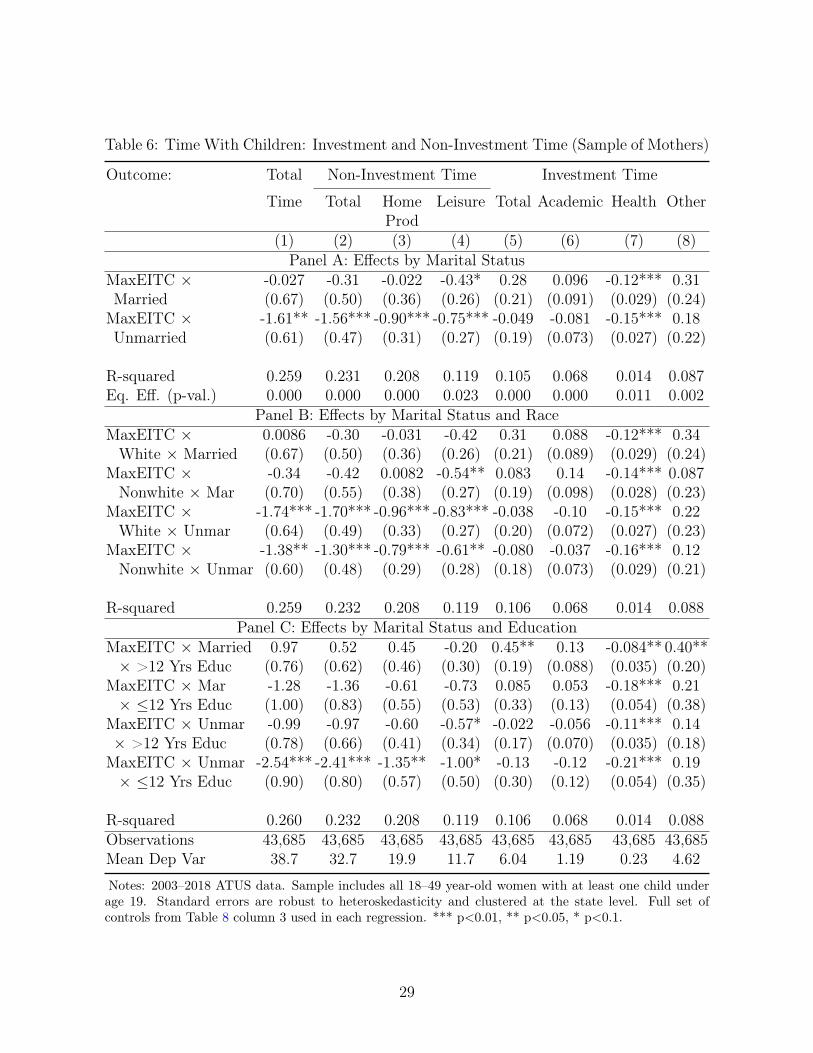
Table 6: Time With Children: Investment and Non-Investment Time (Sample of Mothers)

Outcome: Total Non-Investment Time Investment Time

Time Total Home Leisure Total Academic Health OtherProd

(1) (2) (3) (4) (5) (6) (7) (8)Panel A: Effects by Marital Status

MaxEITC × -0.027 -0.31 -0.022 -0.43* 0.28 0.096 -0.12*** 0.31Married (0.67) (0.50) (0.36) (0.26) (0.21) (0.091) (0.029) (0.24)MaxEITC × -1.61** -1.56*** -0.90*** -0.75*** -0.049 -0.081 -0.15*** 0.18Unmarried (0.61) (0.47) (0.31) (0.27) (0.19) (0.073) (0.027) (0.22)

R-squared 0.259 0.231 0.208 0.119 0.105 0.068 0.014 0.087Eq. Eff. (p-val.) 0.000 0.000 0.000 0.023 0.000 0.000 0.011 0.002

Panel B: Effects by Marital Status and RaceMaxEITC × 0.0086 -0.30 -0.031 -0.42 0.31 0.088 -0.12*** 0.34White × Married (0.67) (0.50) (0.36) (0.26) (0.21) (0.089) (0.029) (0.24)

MaxEITC × -0.34 -0.42 0.0082 -0.54** 0.083 0.14 -0.14*** 0.087Nonwhite × Mar (0.70) (0.55) (0.38) (0.27) (0.19) (0.098) (0.028) (0.23)

MaxEITC × -1.74*** -1.70*** -0.96*** -0.83*** -0.038 -0.10 -0.15*** 0.22White × Unmar (0.64) (0.49) (0.33) (0.27) (0.20) (0.072) (0.027) (0.23)

MaxEITC × -1.38** -1.30*** -0.79*** -0.61** -0.080 -0.037 -0.16*** 0.12Nonwhite × Unmar (0.60) (0.48) (0.29) (0.28) (0.18) (0.073) (0.029) (0.21)

R-squared 0.259 0.232 0.208 0.119 0.106 0.068 0.014 0.088Panel C: Effects by Marital Status and Education

MaxEITC × Married 0.97 0.52 0.45 -0.20 0.45** 0.13 -0.084** 0.40**× >12 Yrs Educ (0.76) (0.62) (0.46) (0.30) (0.19) (0.088) (0.035) (0.20)

MaxEITC × Mar -1.28 -1.36 -0.61 -0.73 0.085 0.053 -0.18*** 0.21× ≤12 Yrs Educ (1.00) (0.83) (0.55) (0.53) (0.33) (0.13) (0.054) (0.38)

MaxEITC × Unmar -0.99 -0.97 -0.60 -0.57* -0.022 -0.056 -0.11*** 0.14× >12 Yrs Educ (0.78) (0.66) (0.41) (0.34) (0.17) (0.070) (0.035) (0.18)MaxEITC × Unmar -2.54*** -2.41*** -1.35** -1.00* -0.13 -0.12 -0.21*** 0.19× ≤12 Yrs Educ (0.90) (0.80) (0.57) (0.50) (0.30) (0.12) (0.054) (0.35)

R-squared 0.260 0.232 0.208 0.119 0.106 0.068 0.014 0.088Observations 43,685 43,685 43,685 43,685 43,685 43,685 43,685 43,685Mean Dep Var 38.7 32.7 19.9 11.7 6.04 1.19 0.23 4.62

Notes: 2003–2018 ATUS data. Sample includes all 18–49 year-old women with at least one child underage 19. Standard errors are robust to heteroskedasticity and clustered at the state level. Full set ofcontrols from Table 8 column 3 used in each regression. *** p<0.01, ** p<0.05, * p<0.1.

29

Table 7: Time-Use Effects: Weekends vs Weekdays

Sample: All Women All Mothers

Outcome: Work Home Prod. Work Home Prod. With Children+ Leisure + Leisure

Total InvestHours Hours

(1) (2) (3) (4) (5) (6)Panel A: Full Sample, Includes Weekends and Weekdays

MaxEITC × 0.77 -0.92* 0.055 -0.40 -0.027 0.28Married (0.46) (0.53) (0.72) (0.80) (0.67) (0.21)MaxEITC × 1.50*** -1.78*** 0.63 -1.32* -1.61** -0.049Unmarried (0.46) (0.51) (0.61) (0.71) (0.61) (0.19)

R-squared 0.184 0.159 0.157 0.122 0.259 0.105Observations 58,090 58,090 43,685 43,685 43,685 43,685Mean Dep Var 26.1 76.0 23.5 79.9 38.7 6.04

Panel B: Restricting Sample to Weekdays (Monday–Friday)MaxEITC × 0.99 -1.32 -0.36 -0.27 -0.46 0.28Married (0.73) (0.80) (1.07) (1.20) (0.77) (0.26)MaxEITC × 2.11*** -2.54*** 0.51 -1.59 -2.52*** -0.18Unmarried (0.70) (0.73) (0.89) (1.11) (0.76) (0.26)

R-squared 0.121 0.115 0.098 0.087 0.245 0.121Observations 28,690 28,690 21,608 21,608 21,608 21,608Mean Dep Var 32.8 70.7 29.6 75.5 35.2 5.91

Panel C: Restricting Sample to Weekends (Saturday–Sunday)MaxEITC × -0.15 0.47 0.55 0.021 1.10 0.32Married (0.48) (0.60) (0.60) (0.70) (1.07) (0.29)MaxEITC × -0.28 0.50 0.59 0.017 0.56 0.28Unmarried (0.53) (0.62) (0.66) (0.63) (0.98) (0.23)

R-squared 0.023 0.068 0.021 0.066 0.240 0.089Observations 29,400 29,400 22,077 22,077 22,077 22,077Mean Dep Var 9.51 88.9 8.49 91.0 47.7 6.35

Notes: 2003–2018 ATUS data. Sample includes all women aged 18–49. Standarderrors are robust to heteroskedasticity and clustered at the state level. Full set ofcontrols from Table 8 column 3 used in each regression. *** p<0.01, ** p<0.05, *p<0.1.

30

Table 8: Estimates Robust to Various Sets of Controls, Sample of All Women

(1) (2) (3) (4) (5) (6) (7) (8)Panel A: Outcome = Labor Force Participation (Mean = 0.78)

MaxEITC × 0.0071 0.0047 0.0050 0.0060 0.0065 0.0080 0.013 0.0070Married (0.0091) (0.0090) (0.0086) (0.0079) (0.0080) (0.0088) (0.0095) (0.013)MaxEITC × 0.031*** 0.030*** 0.030*** 0.031*** 0.031*** 0.033*** 0.039*** 0.032**Unmarried (0.0077) (0.0076) (0.0073) (0.0069) (0.0069) (0.0083) (0.0087) (0.013)

R-squared 0.090 0.103 0.104 0.105 0.106 0.107 0.125 0.108Panel B: Outcome = Weekly Work Hours (Mean = 23.2)

MaxEITC × 0.30 0.27 0.27 0.44 0.46 0.38 0.71* -0.012Married (0.38) (0.36) (0.35) (0.34) (0.34) (0.37) (0.42) (0.38)MaxEITC × 1.19*** 1.20*** 1.20*** 1.37*** 1.38*** 1.30*** 1.63*** 0.90**Unmarried (0.37) (0.37) (0.35) (0.35) (0.35) (0.36) (0.41) (0.38)

R-squared 0.149 0.160 0.161 0.162 0.163 0.164 0.181 0.165Panel C: Outcome = Weekly Home Production + Leisure Hours (Mean = 75.9)

MaxEITC × -0.69 -0.79 -0.92* -1.08** -1.01* -1.10** -1.38** -0.80Married (0.62) (0.62) (0.53) (0.52) (0.51) (0.54) (0.54) (0.62)MaxEITC × -1.56** -1.64*** -1.78*** -1.94*** -1.87*** -1.96*** -2.20*** -1.67**Unmarried (0.60) (0.60) (0.51) (0.49) (0.49) (0.55) (0.53) (0.63)

R-squared 0.149 0.159 0.159 0.161 0.162 0.163 0.182 0.164ControlsYear FE, State FE,#Kids FE X X X X X X X XDemographics X X X X X X X X(Ed FE, Mar) × (St FE, Yr FE) X X X X X X XState-Year Factors X X X X X XState Trend X X X X XState Trend × Unmarried X X X XState-Year Factors × (Kids, Unmarried) X X XState FE × Year FE XYear FE × #Kids FE XObservations 58,090 58,090 58,090 58,090 58,090 58,090 58,090 58,090

Notes: 2003–2018 ATUS data. Sample includes all women aged 18–49. LFP and weekly work hours fromCPS survey data, home production and leisure hours from time-use ATUS data. Standard errors are robust toheteroskedasticity and clustered at the state level. *** p<0.01, ** p<0.05, * p<0.1.

31

Table 9: Estimates Robust to Various Sets of Controls, Sample of Mothers

(1) (2) (3) (4) (5) (6) (7) (8)Panel A: Outcome = Labor Force Participation (Mean = 0.74)

MaxEITC × -0.0050 -0.0077 -0.0060 -0.0054 -0.0056 -0.0096 0.0094 -0.0039Married (0.013) (0.012) (0.011) (0.011) (0.011) (0.011) (0.013) (0.018)MaxEITC × 0.021** 0.022** 0.024** 0.024** 0.024** 0.020* 0.039*** 0.026Unmarried (0.010) (0.0099) (0.0093) (0.010) (0.010) (0.011) (0.012) (0.018)

R-squared 0.079 0.093 0.093 0.095 0.097 0.098 0.121 0.100Panel B: Outcome = Weekly Work Hours (Mean = 21.6)

MaxEITC × -0.25 -0.25 -0.24 0.0087 0.0016 -0.023 0.61 0.16Married (0.46) (0.45) (0.44) (0.44) (0.44) (0.43) (0.58) (0.60)MaxEITC × 0.74* 0.82** 0.83** 1.07*** 1.08*** 1.06*** 1.67*** 1.24**Unmarried (0.40) (0.38) (0.37) (0.39) (0.39) (0.39) (0.49) (0.53)R-squared 0.116 0.131 0.131 0.133 0.134 0.135 0.157 0.137Panel C: Outcome = Weekly Home Production + Leisure Hours (Mean = 79.9)

MaxEITC × -0.11 -0.20 -0.40 -0.62 -0.54 -0.27 -0.65 -0.36Married (0.96) (0.93) (0.80) (0.80) (0.79) (0.74) (0.85) (0.81)MaxEITC × -1.00 -1.12 -1.32* -1.52** -1.45** -1.18* -1.50* -1.29Unmarried (0.87) (0.82) (0.71) (0.72) (0.71) (0.68) (0.76) (0.79)R-squared 0.109 0.121 0.122 0.123 0.125 0.126 0.150 0.128

Panel D: Outcome = Weekly Hours With Children (Mean = 38.7)MaxEITC × 0.068 0.12 -0.027 -0.016 -0.033 -0.16 -0.68 0.30Married (0.73) (0.75) (0.67) (0.68) (0.67) (0.69) (0.91) (0.80)MaxEITC × -1.53** -1.45** -1.61** -1.59** -1.61** -1.70** -2.21** -1.23Unmarried (0.68) (0.68) (0.61) (0.62) (0.62) (0.64) (0.83) (0.77)

R-squared 0.248 0.259 0.259 0.261 0.262 0.262 0.278 0.264Panel E: Outcome = Investment Hours With Children (Mean = 6.0)

MaxEITC × 0.35 0.30 0.28 0.35 0.34 0.33 0.22 0.46Married (0.24) (0.24) (0.21) (0.21) (0.22) (0.23) (0.27) (0.32)MaxEITC × 0.0026 -0.031 -0.049 0.017 0.0065 -0.0071 -0.11 0.13Unmarried (0.23) (0.22) (0.19) (0.19) (0.19) (0.20) (0.23) (0.29)

R-squared 0.098 0.105 0.105 0.107 0.108 0.108 0.127 0.109Controls in Columns 1–8 Are Identical to Those in Table 8Observations 43,685 43,685 43,685 43,685 43,685 43,685 43,685 43,685

Notes: 2003–2018 ATUS data. Sample includes all mothers aged 18–49. LFP and weekly workhours from CPS survey data; home production and leisure hours, hours with children, and invest-ment with children from time-use ATUS data. Standard errors are robust to heteroskedasticityand clustered at the state level. *** p<0.01, ** p<0.05, * p<0.1.

32

Table 10: EITC Effects by Predicted Probability of Low Income

Outcome: LFP Hours with Hours Hours HomeChildren Investing Production

in Children and Leisure(1) (2) (3) (4)

MaxEITC × Low -0.0043 0.33 0.40* -0.28× Married (0.010) (0.74) (0.24) (0.82)MaxEITC × Med -0.0070 -0.30 0.25 -0.42× Married (0.011) (0.70) (0.22) (0.87)MaxEITC × High -0.0010 -0.82 0.069 -1.33*× Married (0.015) (0.78) (0.27) (0.99)MaxEITC × Low 0.018** -1.44** -0.13 -1.00× Unmarried (0.0076) (0.66) (0.18) (0.70)MaxEITC × Med 0.021** -2.14*** -0.21 -1.47*× Unmarried (0.0095) (0.67) (0.21) (0.74)MaxEITC × High 0.030** -2.07*** -0.10 -2.04**× Unmarried (0.013) (0.69) (0.24) (0.91)

R-squared 0.093 0.260 0.106 0.122Observations 43,685 43,685 43,685 43,685

Notes: 2003–2018 ATUS data. Sample includes all mothers aged 18–49. Tocreate terciles (Low, Med, High) for predicted probability of low earnings, wefirst regress an indicator for household earnings less than $20,000 on a set ofcontrols (year FE, state FE, number of kids FE, 4 education categories, black,hispanic, age, and birth year) using ATUS weights. Then, the predicted prob-abilities are used to categorize individuals into terciles, where the cutoffs areprobabilities 0.12 and 0.24. Among married mothers, 40, 35, and 25 percentare in terciles 1, 2, and 3, respectively. Among unmarried mothers, 25, 32, and44 percent are in terciles 1, 2, and 3, respectively. The outcome regressionscontrol for predicted probability tercile FE and the full set of controls from Ta-ble 8 column 4. Standard errors are robust to heteroskedasticity and clusteredat the state level. *** p<0.01, ** p<0.05, * p<0.1.

33

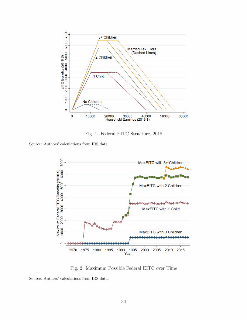
Fig. 1. Federal EITC Structure, 2018

Source: Authors’ calculations from IRS data.

Fig. 2. Maximum Possible Federal EITC over Time

Source: Authors’ calculations from IRS data.

34

Fig. 3. State EITC Rates (as a Fraction of Federal Benefits) over Time

Notes: Authors’ calculations from NBER data. https://users.nber.org/~taxsim/state-eitc.html.Although CA has a high match rate, it only matches up to half of the maximum federal EITC benefit, so inour regressions we divide the CA state EITC rate by two.

35

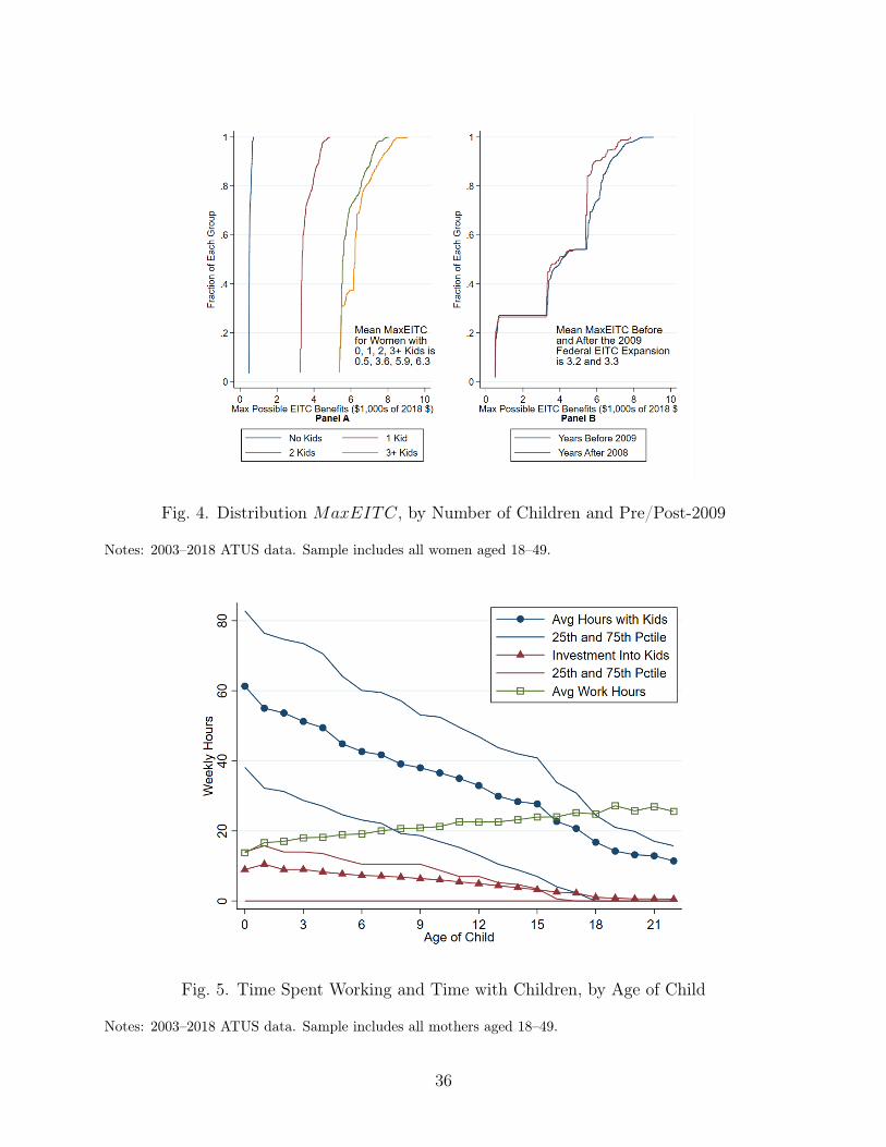
Fig. 4. Distribution MaxEITC, by Number of Children and Pre/Post-2009

Notes: 2003–2018 ATUS data. Sample includes all women aged 18–49.

Fig. 5. Time Spent Working and Time with Children, by Age of Child

Notes: 2003–2018 ATUS data. Sample includes all mothers aged 18–49.

36

Fig. 6. Effect of the EITC on Time-Use among Unmarried Mothers: Prob(Hours > X)

Notes: 2003–2018 ATUS data. Sample includes all mothers aged 18–49. Each estimate comes from a separateregression using equation (3). Work hours in Panel A come from CPS survey data; outcomes in Panels B–Dcome from ATUS data, which asks about time-use in a single day and we scale these to weekly hours. Full setof controls from Table 8 column 3 used in each regression. Standard errors are robust to heteroskedasticityand clustered at the state level.

37

Fig. 7. EITC Effect on LFP and Time Spent with Children, by Mothers’ Age

Notes: 2003–2018 ATUS data. Sample includes all mothers aged 18–49. Each estimate comes from asingle regression resembling equation (1), except “MaxEITC × Unmarried” and “MaxEITC × Married” areinteracted with six binary age categories of the mother. Full set of controls from Table 8 column 3 used ineach regression. Standard errors are robust to heteroskedasticity and clustered at the state level.

38

Fig. 8. Effects of the EITC on Time with Children, by Age of Children

Notes: 2003–2018 ATUS data. Sample includes all mothers aged 18–49. Estimates from equation (4). Fullset of controls from Table 8 column 3 used in each regression. Standard errors are robust to heteroskedasticityand clustered at the state level.

39

Appendix A: Additional Tables and Figures

1

Table A.1: Labor Supply, Earnings, and EITC Benefits, by Race and Education

Outcome: LFP Weekly EITC Any Earnings EarningsWork Benefits EITC and EITCHours

(1) (2) (3) (4) (5) (6)Panel A: Effects by Marital Status and Race

MaxEITC × -0.0054 -0.26 233.1*** 0.0041 421.9 655.0White × Married (0.011) (0.45) (36.1) (0.0096) (545.9) (537.7)

MaxEITC × -0.0081 -0.049 262.1*** 0.0099 539.1 801.2Nonwhite × Married (0.0097) (0.42) (36.9) (0.0090) (533.4) (537.2)

MaxEITC × 0.028*** 0.99*** 338.3*** 0.014 1449.2*** 1787.4***White × Unmarried (0.0094) (0.37) (35.2) (0.0098) (509.1) (509.9)

MaxEITC × 0.016 0.54 401.8*** 0.031*** 822.7 1224.5**Nonwhite × Unmarried (0.010) (0.39) (37.1) (0.0090) (536.4) (543.3)

R-squared 0.094 0.132 0.285 0.292 0.213 0.201Eq. Eff. (p-val.) 0.000 0.000 0.000 0.000 0.000 0.000

Panel B: Effects by Marital Status and EducationMaxEITC × Married -0.0095 -0.59 89.7** -0.0049 951.7 1041.3× >12 Yrs Educ (0.010) (0.37) (43.2) (0.0088) (780.5) (795.8)

MaxEITC × Married -0.00051 0.21 427.3*** 0.017 -255.2 172.1× ≤12 Yrs Educ (0.021) (0.77) (64.4) (0.021) (546.6) (526.0)

MaxEITC × Unmarried 0.016 0.53 251.1*** 0.018** 1634.6** 1885.7**× >12 Yrs Educ (0.012) (0.37) (43.6) (0.0080) (785.0) (802.9)MaxEITC × Unmarried 0.032* 1.24* 518.0*** 0.025 640.1 1158.0**× ≤12 Yrs Educ (0.018) (0.69) (62.1) (0.020) (472.0) (465.1)

R-squared 0.093 0.131 0.287 0.292 0.213 0.200Eq. Eff. (p-val.) 0.000 0.000 0.000 0.000 0.000 0.000Observations 43,685 43,685 43,685 43,685 43,685 43,685Mean Dep Var 0.74 21.6 1021.9 0.34 23514.9 24536.9

Notes: 2003–2018 ATUS data. Sample includes all mothers aged 18–49. Outcomes are based onCPS data. Standard errors are robust to heteroskedasticity and clustered at the state level. Fullset of controls from Table 8 column 3 used in each regression. *** p<0.01, ** p<0.05, * p<0.1.

2

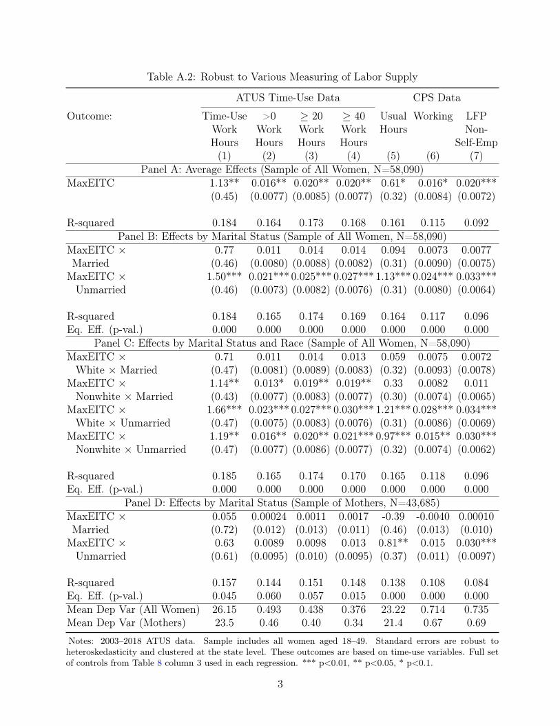
Table A.2: Robust to Various Measuring of Labor Supply

ATUS Time-Use Data CPS Data

Outcome: Time-Use >0 ≥ 20 ≥ 40 Usual Working LFPWork Work Work Work Hours Non-Hours Hours Hours Hours Self-Emp(1) (2) (3) (4) (5) (6) (7)

Panel A: Average Effects (Sample of All Women, N=58,090)MaxEITC 1.13** 0.016** 0.020** 0.020** 0.61* 0.016* 0.020***

(0.45) (0.0077) (0.0085) (0.0077) (0.32) (0.0084) (0.0072)

R-squared 0.184 0.164 0.173 0.168 0.161 0.115 0.092Panel B: Effects by Marital Status (Sample of All Women, N=58,090)

MaxEITC × 0.77 0.011 0.014 0.014 0.094 0.0073 0.0077Married (0.46) (0.0080) (0.0088) (0.0082) (0.31) (0.0090) (0.0075)MaxEITC × 1.50*** 0.021*** 0.025*** 0.027*** 1.13*** 0.024*** 0.033***Unmarried (0.46) (0.0073) (0.0082) (0.0076) (0.31) (0.0080) (0.0064)

R-squared 0.184 0.165 0.174 0.169 0.164 0.117 0.096Eq. Eff. (p-val.) 0.000 0.000 0.000 0.000 0.000 0.000 0.000

Panel C: Effects by Marital Status and Race (Sample of All Women, N=58,090)MaxEITC × 0.71 0.011 0.014 0.013 0.059 0.0075 0.0072White × Married (0.47) (0.0081) (0.0089) (0.0083) (0.32) (0.0093) (0.0078)

MaxEITC × 1.14** 0.013* 0.019** 0.019** 0.33 0.0082 0.011Nonwhite × Married (0.43) (0.0077) (0.0083) (0.0077) (0.30) (0.0074) (0.0065)

MaxEITC × 1.66*** 0.023*** 0.027*** 0.030*** 1.21*** 0.028*** 0.034***White × Unmarried (0.47) (0.0075) (0.0083) (0.0076) (0.31) (0.0086) (0.0069)

MaxEITC × 1.19** 0.016** 0.020** 0.021*** 0.97*** 0.015** 0.030***Nonwhite × Unmarried (0.47) (0.0077) (0.0086) (0.0077) (0.32) (0.0074) (0.0062)

R-squared 0.185 0.165 0.174 0.170 0.165 0.118 0.096Eq. Eff. (p-val.) 0.000 0.000 0.000 0.000 0.000 0.000 0.000

Panel D: Effects by Marital Status (Sample of Mothers, N=43,685)MaxEITC × 0.055 0.00024 0.0011 0.0017 -0.39 -0.0040 0.00010Married (0.72) (0.012) (0.013) (0.011) (0.46) (0.013) (0.010)MaxEITC × 0.63 0.0089 0.0098 0.013 0.81** 0.015 0.030***Unmarried (0.61) (0.0095) (0.010) (0.0095) (0.37) (0.011) (0.0097)

R-squared 0.157 0.144 0.151 0.148 0.138 0.108 0.084Eq. Eff. (p-val.) 0.045 0.060 0.057 0.015 0.000 0.000 0.000Mean Dep Var (All Women) 26.15 0.493 0.438 0.376 23.22 0.714 0.735Mean Dep Var (Mothers) 23.5 0.46 0.40 0.34 21.4 0.67 0.69

Notes: 2003–2018 ATUS data. Sample includes all women aged 18–49. Standard errors are robust toheteroskedasticity and clustered at the state level. These outcomes are based on time-use variables. Full setof controls from Table 8 column 3 used in each regression. *** p<0.01, ** p<0.05, * p<0.1.

3

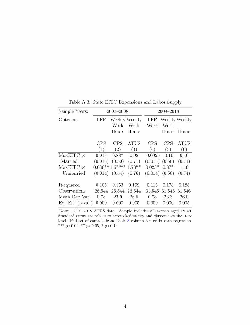
Table A.3: State EITC Expansions and Labor Supply

Sample Years: 2003–2008 2009–2018

Outcome: LFP Weekly Weekly LFP WeeklyWeeklyWork Work Work WorkHours Hours Hours Hours

CPS CPS ATUS CPS CPS ATUS(1) (2) (3) (4) (5) (6)

MaxEITC × 0.013 0.88* 0.98 -0.0025 -0.16 0.46Married (0.013) (0.50) (0.71) (0.015) (0.50) (0.71)MaxEITC × 0.036** 1.67*** 1.73** 0.023* 0.87* 1.16Unmarried (0.014) (0.54) (0.76) (0.014) (0.50) (0.74)

R-squared 0.105 0.153 0.199 0.116 0.178 0.188Observations 26,544 26,544 26,544 31,546 31,546 31,546Mean Dep Var 0.78 23.9 26.5 0.78 23.3 26.0Eq. Eff. (p-val.) 0.000 0.000 0.005 0.000 0.000 0.005

Notes: 2003–2018 ATUS data. Sample includes all women aged 18–49.Standard errors are robust to heteroskedasticity and clustered at the statelevel. Full set of controls from Table 8 column 3 used in each regression.*** p<0.01, ** p<0.05, * p<0.1.

4

Table A.4: The EITC and Decomposing All Time-Use (168 Weekly Hours)

Outcome: Home Production Leisure Work School Sleep Uncat.

With Children? Yes No Yes No(1) (2) (3) (4) (5) (6) (7) (8) (9) (10)

Panel A: Effects by Marital Status and RaceMaxEITC × -0.37 -0.036 -0.33 0.018 -0.11 0.13 0.030 0.11 0.20 0.011White × Married (0.61) (0.40) (0.38) (0.51) (0.37) (0.45) (0.73) (0.27) (0.36) (0.086)

MaxEITC × -0.16 0.033 -0.20 -0.66 -0.48 -0.18 0.34 0.087 0.40 0.0034Nonwhite × Married (0.60) (0.41) (0.39) (0.51) (0.38) (0.46) (0.69) (0.27) (0.37) (0.087)

MaxEITC × -1.11** -1.25*** 0.14 -0.39 -0.58 0.19 0.87 0.17 0.45 0.011White × Unmarried (0.51) (0.37) (0.34) (0.54) (0.37) (0.52) (0.62) (0.30) (0.49) (0.11)

MaxEITC × -0.55 -1.02*** 0.47 -0.47 -0.46 -0.011 0.23 0.20 0.57 0.017Nonwhite × Unmarried (0.54) (0.31) (0.38) (0.60) (0.35) (0.59) (0.64) (0.30) (0.47) (0.11)

R-squared 0.117 0.222 0.077 0.113 0.144 0.141 0.158 0.133 0.113 0.024Panel B: Effects by Marital Status and Education

MaxEITC × Married -0.26 0.49 -0.75** 0.16 0.20 -0.046 -0.90 0.54** 0.38 0.077× >12 Yrs Educ (0.60) (0.55) (0.34) (0.50) (0.36) (0.47) (0.84) (0.23) (0.38) (0.096)

MaxEITC × Married -0.45 -0.67 0.22 -0.35 -0.59 0.24 1.35 -0.52 0.048 -0.074× ≤12 Yrs Educ (1.00) (0.57) (0.60) (1.07) (0.71) (0.79) (1.32) (0.47) (0.48) (0.14)

MaxEITC × Unmarried -0.68 -0.83 0.15 -0.28 -0.36 0.085 -0.45 0.81*** 0.53 0.057× >12 Yrs Educ (0.56) (0.51) (0.35) (0.59) (0.37) (0.55) (0.95) (0.28) (0.48) (0.10)MaxEITC × Unmarried -1.16 -1.68*** 0.52 -0.61 -0.81 0.20 2.00* -0.58 0.40 -0.051× ≤12 Yrs Educ (0.93) (0.56) (0.56) (1.06) (0.66) (0.87) (1.12) (0.47) (0.57) (0.17)

Observations 43,685 43,685 43,685 43,685 43,685 43,685 43,685 43,685 43,685 43,685Mean Dep Var (Mothers) 46.5 22.0 24.4 33.4 15.6 17.8 23.5 2.18 60.9 1.49

Notes: 2003–2018 ATUS data. Sample includes all mothers aged 18–49. Standard errors are robust to heteroskedas-ticity and clustered at the state level. The six categories are mutually exclusive and sum to 168 weekly hours. TablesA.6 and A.7 further decompose home production and leisure with children from columns 2 and 5. Full set of controlsfrom Table 8 column 3 used in each regression. *** p<0.01, ** p<0.05, * p<0.1.

5

Table A.5: Outcomes Robust to EITC Definition

Outcome: LFP Work Home Prod. Time with InvestingHours and Leisure Children in Children

Hours Hours Hours(1) (2) (3) (4) (5)

Panel A: Sample = All WomenEITC Phase-In Rate 0.0020 0.064 -1.08× Married (0.012) (0.47) (0.80)

EITC Phase-In Rate 0.037*** 1.41*** -2.26***× Unmarried (0.010) (0.48) (0.77)

R-squared 0.103 0.160 0.159Observations 58,090 58,090 58,090

Panel B: Sample = All MothersEITC Phase-In Rate -0.019 -0.81 -0.27 0.49 0.47× Married (0.015) (0.60) (1.21) (0.89) (0.31)

EITC Phase-In Rate 0.033*** 1.18** -1.62 -2.92*** -0.21× Unmarried (0.012) (0.53) (1.10) (0.78) (0.28)

R-squared 0.093 0.131 0.122 0.260 0.105Observations 43,685 43,685 43,685 43,685 43,685

Notes: 2003–2018 ATUS data. Sample includes all women or all mothers aged 18–49. Units are10 percentage points. The following example illustrates the phase-in rate: if the federal phase-in rate is 40 percent and the state EITC matches 20 percent of the federal EITC, then thetotal phase-in rate is 0.40(1+0.20)=0.48. Standard errors are robust to heteroskedasticity andclustered at the state level. Full set of controls from Table 8 column 3 used in each regression.*** p<0.01, ** p<0.05, * p<0.1.

6

Table A.6: Decomposing Home Production with Kids (from Table 5 Column 2)

Outcome: Personal House- Food Waiting, Caring Civic Eating Errands,Care work Prep Shop- for Travel

ping Others(1) (2) (3) (4) (5) (6) (7) (8)

MaxEITC × -0.069* 0.042 0.025 -0.087 0.024 -0.0074 0.11 -0.044Married (0.035) (0.16) (0.041) (0.30) (0.046) (0.0066) (0.091) (0.061)MaxEITC × -0.11** -0.23* 0.029 -0.19 -0.0034 -0.0069 -0.015 -0.19***Unmarried (0.049) (0.15) (0.040) (0.29) (0.026) (0.0057) (0.088) (0.046)

R-squared 0.019 0.082 0.013 0.158 0.014 0.020 0.156 0.059Eq. Eff. (p-val.) 0.257 0.000 0.683 0.036 0.404 0.841 0.011 0.001Full Controls X X X X X X X XObservations 43,685 43,685 43,685 43,685 43,685 43,685 43,685 43,685Mean Dep Var 0.24 3.48 0.11 6.48 0.12 0.013 4.09 2.85

Notes: 2003–2018 ATUS data. Sample includes all 18–49 year-old mothers. Standard errors arerobust to heteroskedasticity and clustered at the state level. Full set of controls from Table 8column 3 used in each regression. *** p<0.01, ** p<0.05, * p<0.1.

Table A.7: Decomposing Leisure with Kids (from Table 5 Column 5)

Outcome: Activities Educ Socializing Sports ReligiousVolunteer Phone Travelwith & Relaxing

Children(1) (2) (3) (4) (5) (6) (7) (8)

MaxEITC × 0.13 0.0037 -0.43* 0.053 -0.013 0.0025 0.055*** 0.043Married (0.17) (0.0081) (0.25) (0.052) (0.047) (0.042) (0.020) (0.035)MaxEITC × 0.094 0.0030 -0.58** 0.038 -0.051 -0.074 0.039** 0.0035Unmarried (0.17) (0.0085) (0.25) (0.051) (0.049) (0.055) (0.017) (0.036)

R-squared 0.087 0.011 0.097 0.024 0.055 0.016 0.022 0.050Eq. Eff. (p-val.) 0.456 0.756 0.202 0.468 0.028 0.001 0.053 0.004Full Controls X X X X X X X XObservations 43,685 43,685 43,685 43,685 43,685 43,685 43,685 43,685Mean Dep Var 2.98 0.017 10.2 0.63 0.52 0.33 0.14 0.78

Notes: 2003–2018 ATUS data. Sample includes all 18–49 year-old mothers. Standard errors are robust toheteroskedasticity and clustered at the state level. Full set of controls from Table 8 column 3 used in eachregression. *** p<0.01, ** p<0.05, * p<0.1.

7

Table A.8: Decomposing Health and “Other” Investment in Kids” (Table 6 columns 7 and 8)

Health Investment Other Investment

Provide Obtain Arts Talk Organize Look AttendMedical Medical Play and Sports and and After EventsCare Care Crafts Listen Plan Kids(1) (2) (3) (4) (5) (6) (7) (8) (9)

MaxEITC × -0.068** -0.055* 0.16 0.0022 0.051 -0.040 0.0069 0.085 0.041Married (0.023) (0.028) (0.15) (0.013) (0.052) (0.038) (0.012) (0.075) (0.062)MaxEITC × -0.085*** -0.068** 0.24** 0.0049 0.032 -0.064* -0.0016 0.026 -0.051Unmarried (0.022) (0.026) (0.14) (0.013) (0.051) (0.038) (0.012) (0.083) (0.046)

R-squared 0.010 0.016 0.082 0.013 0.020 0.037 0.016 0.029 0.029Eq. Eff. (p-val.) 0.013 0.253 0.067 0.678 0.326 0.044 0.049 0.005 0.000Unmarried vs Mar -0.017** -0.012 0.076* 0.0027 -0.019 -0.024** -0.0085** -0.059*** -0.092***Difference (0.0070) (0.011) (0.041) (0.0064) (0.019) (0.012) (0.0043) (0.021) (0.020)

Observations 43,685 43,685 43,685 43,685 43,685 43,685 43,685 43,685 43,685Mean Dep Var 0.11 0.12 2.28 0.075 0.56 0.41 0.078 0.60 0.63

Notes: 2003–2018 ATUS data. Sample includes all 18–49 year-old mothers. Standard errors are robust to het-eroskedasticity and clustered at the state level. Full set of controls from Table 8 column 3 used in each regression.*** p<0.01, ** p<0.05, * p<0.1.

8

Fig. A.1. Maximum Possible Federal + State EITC over Time

Source: Authors’ calculations from IRS and NBER data. Each point denotes a state by year value.

Fig. A.2. CDF of Weekly Work Hours, by Number of Children

Notes: 2003–2018 ATUS data. Sample includes all women aged 18–49. Weekly work hours from CPS hoursworked last week.

9

Fig. A.3. CDF of Home-Production Hours, by Number of Children

Notes: 2003–2018 ATUS data. Sample includes all women aged 18–49. Home production hours from ATUSdata, which asks about time-use in a single day (scaled to weekly hours).

Fig. A.4. CDF of Weekly Leisure Hours, by Number of Children

Notes: 2003–2018 ATUS data. Sample includes all women aged 18–49. Leisure hours comes from ATUSdata, which asks about time-use in a single day (scaled to weekly hours).

10

Fig. A.5. CDF of Weekly Hours with Children, by Number of Children

Notes: 2003–2018 ATUS data. Sample includes all women aged 18–49. Time with kids comes from ATUSdata, which asks about time-use in a single day (scaled to weekly hours).

Fig. A.6. CDF of Weekly Hours Invested in Children, by Number of Children

Notes: 2003–2018 ATUS data. Sample includes all women aged 18–49. Investment hours comes from ATUSdata, which asks about time-use in a single day (scaled to weekly hours).

11

Fig. A.7. EITC Effect on Time-Use by Unmarried Women: Prob(Hours > X)

Notes: 2003–2018 ATUS data. Sample includes all women aged 18–49. Figure identical to Figure 6 PanelsA-D except the sample includes all women. Standard errors are robust to heteroskedasticity and clusteredat the state level. Full set of controls from Table 8 column 3 used in each regression.

12

Data Appendix: ATUS Data Activity Lexicon (2003)

This appendix provides a detailed description of how we categorized all ATUS time-useactivities.

The American Time Use Survey (ATUS) is a comprehensive survey of time use in theU.S. and has been administered annually since 2003. The ATUS sample is drawn from theCurrent Population Surveys (CPS), covering the population of non-institutionalized civiliansat least 15 years old. Typical sample sizes have been about 26,000 respondents since 2004with surveys administered evenly throughout the year. We use sample weights designed toadjust for stratified sampling, non-response, and to get a representative measure for eachday of the year.

The survey asks individuals detailed information about all of their activities over theprevious day, including who they were with at the time. The survey also collects informationabout the respondent and household. It can be linked with the CPS data. Our analysiscombines data from the 2003–2018 surveys.

The following provides a detailed breakdown of how we categorized all ATUS time-useactivities based on the 2003 ATUS Data Activity Lexicon.

HOME PRODUCTION:01 Personal Care

01.02 Grooming - all01.03 Health-related Self Care - all01.05 Personal Care Emergencies - all01.99 Personal Care, n.e.c* - all

02 Household Activities02.01 Housework - all02.02 Food and Drink Preparation, Presentation, and Clean-up - all02.03 Interior Maintenance, Repair, and Decoration - all02.04 Exterior Maintenance, Repair, and Decoration - all02.05 Lawn, Garden, and Houseplants - all02.06 Animals and Pets - all02.07 Vehicles - all02.08 Appliances and Tools - all02.09 Household Management - all02.99 Household Activities, n.e.c* - all

03 Caring For and Helping Household Members03.01 Caring For and Helping Household Children

03.01.01 Physical care for household children03.01.06 Talking with/listening to household children03.01.07 Helping/teaching household children (not related to education)03.01.08 Organization and planning for household children03.01.09 Looking after household children (as a primary activity)03.01.10 Waiting for/with household children03.01.11 Picking up/dropping off household children (as a primary activity)

13

03.01.99 Caring for and helping household children, n.e.c.*03.02 Activities Related to household Children’s Education - all03.03 Activities Related to household Children’s Health - all03.04 Caring for Household Adults - all03.05 Helping Household Adults - all03.99 Caring for and Helping Household Members, n.e.c.* - all

04 Caring For and Helping Nonhousehold Members04.01 Caring For and Helping nonhousehold Children

04.01.01 Physical care for nonhousehold children04.01.06 Talking with/listening to nonhousehold children04.01.07 Helping/teaching nonhousehold children (not related to education)04.01.08 Organization and planning for nonhousehold children04.01.09 Looking after nonhousehold children (as primary activity)04.01.11 Waiting for/with nonhousehold children

07 Consumer Purchases - all08 Professional and Personal Care Services - all09 Household Services - all10 Government Services and Civic Obligations - all11 Eating and Drinking - all16 Telephone Calls

16.01 Telephone Calls (to or from)16.01.03 Telephone calls to/from education services providers16.01.04 Telephone calls to/from salespeople16.01.05 Telephone calls to/from professional or pers. care svcs providers16.01.06 Telephone calls to/from household services providers16.01.07 Telephone calls to/from paid child or adult care providers16.01.08 Telephone calls to/from government officials

16.99 Telephone Calls, n.e.c* - all17 Traveling

17.01 Travel Related to Personal Care - all17.02 Travel Related to Household Activities - all17.03 Travel Related to Caring For and Helping household Members - all17.04 Travel Related to Caring For and Helping Nonhousehold Members - all17.07 Travel Related to Consumer Purchases - all17.08 Travel Related to Using Professional and Personal Care Services - all17.09 Travel Related to Using Household Services - all17.10 Travel Related to Using Government Services and Civic Obligations - all17.11 Travel Related to Eating and Drinking - all17.16 Travel Related to Telephone Calls - all17.17 Security Procedures Related to Traveling - all17.99 Travel n.e.c.* - all

14

SCHOOL:06 Education

06.01 Taking Class06.01.01 Taking class: degree06.01.03 Waiting associated with taking classes06.01.04 Security procedures related to taking classes06.01.99 Taking class, n.e.c.*

06.03 Research/Homework06.03.01 Research/homework: class for degree06.03.03 Waiting associated with research/homework06.03.99 Research/homework n.e.c*

06.04 Registration/Administrative Activities06.04.01 Administrative activities: class for degree06.04.03 Waiting associated with administrative activities (education)06.04.99 Administrative for education, n.e.c*

06.99 Education, n.e.c* - all17 Traveling

17.06 Travel Related to Education - all

WORK:05 Working and Work-Related Activities - all17 Traveling

17.05 Travel Related to Work - all

LEISURE:01 Personal Care

01.04 Personal Activities - all03 Caring For and Helping Household Members

03.01 Caring For and Helping Household Children03.01.02 Reading to/with household children03.01.03 Playing with household children, not sports03.01.04 Arts and crafts with household children03.01.05 Playing sports with household children03.01.10 Attending household children’s events

04 Caring For and Helping Nonhousehold Members04.01 Caring For and Helping nonhousehold Children

04.01.02 Reading to/with nonhousehold children04.01.03 Playing with nonhousehold children04.01.04Arts and crafts with nonhousehold children04.01.05 Playing sports with nonhousehold children04.01.10 Attending nonhousehold children’s events04.01.12 Dropping off/picking up nonhousehold children

15

04.01.99 Caring for nonhousehold children n.e.c.*04.02 Activities Related to Nonhousehold Children’s Education - all04.03 Activities Related to Nonhousehold Children’s Health - all04.04 Caring For Nonhousehold Adults - all04.05 Helping Nonhousehold Adults - all04.99 Caring for and Helping Nonhousehold Members, n.e.c.* - all

06 Education06.01 Taking Class

06.01.02 Taking class: personal interest06.02 Extracurricular School Activities (Except Sports) - all06.03 Research/Homework

06.03.02 Research/homework: class for personal interest06.04 Registration/Administrative Activities

06.04.02 Administrative activities: class for personal interest12 Socializing, Relaxing, and Leisure - all13 Sports, Exercise, and Recreation - all14 Religious and Spiritual Activities - all15 Volunteer Activities - all16 Telephone Calls

16.01 Telephone Calls (to or from)16.01.01 Telephone calls to/from family members16.01.21 Telephone calls to/from friends, neighbors, or acquaintances

17 Traveling17.12 Travel Related to Socializing, Relaxing, and Leisure - all17.13 Travel Related to Sports, Exercise, and Recreation - all17.14 Travel Related to Religious/Spiritual Activities - all17.15 Travel Related to Volunteer Activities - all

UNCATEGORIZED:01 Personal Care

01.01 Sleeping - all50 Data Codes - all

INVESTMENT TIMEOur measure of child time investment sums all of the time parents report spending with

children in each of the following activities (each categorized as either home production orleisure as above):

(03.01) Caring For and Helping Household Children: (03.01.02) Reading to/with householdchildren; (03.01.03) Playing with household children, not sports; (03.01.04) Arts and craftswith household children; (03.01.05) Playing sports with household children; (03.01.06) Talk-ing with/listening to household children; (03.01.07) Helping/teaching household children(not related to education); (03.01.08) Organization and planning for household children;

16

(03.01.09) Looking after household children (as a primary activity; (03.01.10) Attendinghousehold children’s events.

(03.02) Activities Related to Household Children’s Education: (03.02.01) Homework (house-hold children); (03.02.02) Meetings and School Conferences (household children); (03.02.03)Home schooling of household children.

(03.03) Activities Related to Household Children’s Health: (03.03.01) Providing medical careto household children; (03.03.02) Obtaining medical care for household children.

(12.03) Relaxing and Leisure: (12.03.07) Playing games; (12.03.09) Arts and crafts as ahobby.

(12.04) Arts and Entertainment (other than sports): (12.04.01) Attending performing arts;(12.04.02) Attending museum; (12.04.03) Attending movies/film.

(13.01) Participating in Sports, Exercise, and Recreation: all subcategories.

17