The E3-India Model Manual: Volume 3 - Cambridge …€¦ · · 2017-08-11series covering the...

This volume (3) is part of an 9-volume

series covering the E3-India model

manual

June

2017

Cambridge Econometrics

Cambridge, UK

[email protected]

www.camecon.com

The Regulatory Assistance Project

The E3-India Model Technical model manual, Volume 3:

Data and Model Validation

The E3-India Model Manual: Volume 3

2 Cambridge Econometrics

Cambridge Econometrics’ mission is to provide rigorous, accessible and relevant independent

economic analysis to support strategic planners and policy-makers in business and government, doing

work that we are interested in and can be proud of.

Cambridge Econometrics Limited is owned by a charitable body,

the Cambridge Trust for New Thinking in Economics.

www.neweconomicthinking.org

http://www.neweconomicthinking.org/

Authorisation and Version History

Version Date Authorised

for release by

Description

1.0 17/06/17 Hector Pollitt First version, volume 3.



Contents

Page

1 Model Inputs and Outputs 5

1.1 Introduction 5

1.2 Data inputs 5

1.3 Econometric parameters 10

1.4 Baseline forecast 11

1.5 Other model inputs 12

1.6 Model outputs 14



1 Model Inputs and Outputs

1.1 Introduction

This volume describes E3-India’s main model inputs and outputs. The following

sections describe the main inputs that the model relies on, including data and

econometric parameters. The final part of Chapter 1 describes the format of the

main model outputs.

Chapter 2 in this volume describes the intensive model validation exercise that

has been undertaken. The appendices provide a list of model inputs, outputs

and classifications.

1.2 Data inputs

The data are the most important single input to E3-India. A lot of effort is put

into ensuring that the model data are accurate and consistent to the maximum

degree possible.

The following databanks are used to store the data:

• T – historical time-series data

• F – processed baseline forecast (see Section 4)

• X – cross-section data, including input-output tables and equation

parameters

• E – energy balances, prices and emissions

• U – classification titles

One other databank is used for model operation:

• S – holds the calibration factors to match the baseline forecast (see section

4)

E3-India’s data requirements are extensive and specific. All data must be

processed so that they are in the correct classifications and units. Gaps in the

data must be filled (see below). All data processing is carried out using the

Oxmetrics software package.

It is a substantial exercise to create and maintain the time series of economic

data. The main dimensions involved are:

• indicator

• states

• sector

• time period (annually from 1993)

In addition, indicators that are expressed in monetary units have constant and

current price versions. Cambridge Econometrics therefore puts a large amount

of resources into processing the time-series data.

Introduction to the model databanks

Time-series economic data

http://www.oxmetrics.net/pages/software.html



The raw data are gathered from the sources described below and stored on the

T databank. The model uses official sources as much as possible. It is often

necessary to combine data sets to fill out gaps in the data and to estimate

remaining missing values (see below).

A ‘V’ at the start of the name indicates a current price value; otherwise the

indicator is expressed in constant prices (2010 rupees). The main indicators

with full sectoral disaggregation are:

• QR/VQR – output (constant and current price bases)

• YVM/VYVM, YVF/VYVF – GVA at market prices and factor cost

• KR/VKR – investment

• CR/VCR – household expenditure (by product)

• GR/VGR – government final consumption (by category)

• QRX/VQRX – exports

• QRM/VQRM – imports

• YRE – employment

• YRLC – labour costs (current prices)

There are also time series for population (DPOP) and labour force (LGR),

disaggregated by age and gender.

In addition, there are several macro-level time series that are used in the

modelling. These include GDP, household incomes, tax and interest rates and

the unemployment rate. They are also collected on an annual basis, starting

from 1993.

Table 1-1 gives a summary of the data sources for economic variables used in

the E3-India model.

The data must be consistent across states and in the same units. For monetary

data, the rupee is used.

Table 1-1: E3-India data sources for economic variables

Variable Source

Population Census of India

MOSPI Net State domestic product series

Unemployment and labour

participation rates

NSSO Employment and Unemployment in India

Surveys

NSSO Employment and Unemployment Situation in

India Surveys

NSSO Household expenditure and Employment

Situation in India Surveys

Employment NSSO Employment and Unemployment in India

Surveys

NSSO Employment and Unemployment Situation in

India Surveys

The main

indicators

Data sources for

E3-India’s

economic data



NSSO Household expenditure and Employment

Situation in India Surveys

Gross output and value added MOSPI Gross State domestic product 1993-2006,

1999-2010, 2004-14

MOSPI Gross State value added 2011-2015

MOSPI Mining production by state and product 2009-

13

Own estimation using information from national total

Consumer expenditure NSSO Household Consumer Expenditure in India

NSSO Household Consumer Expenditure and

Employment situation

NSSO Key Indicators of Household Consumer

Expenditure in India

NSSO Level and Pattern of Consumer Expenditure

E3 India state rural and urban population

Government spending Reserve Bank of India State Finances: A Study of

Budgets

India Ministry of Finance Union Budgets

E3 India Population

Own estimation using information from national total

Investment Own estimation using information from national total

(share of investment in national accounts)

External trade Own estimation using information from national total

(share of trade in national accounts)

Total gross disposable income Own estimation using information from national total

(ratio of gross disposable income and total wages and

salaries in national accounts)

MOSPI – Indian Ministry of Statistics and Programme Implementation NSSO – Indian National Sample survey reports

The general principle adopted in E3-India is that variables are defined in the

currency unit appropriate for the use of the variable. This usually means that the

units of measurement follow those in the data source. The principle of

comparability is taken to imply that most current values are measured in millions

of rupees and most constant values in millions of rupees at 2010 prices.

The price indices are calculated by dividing current by constant values in

rupees.

By cross-sectional data we mean data that are not usually available in time-

series format. Historically, this has meant input-output tables. Other cross-

sectional data include converters between model classifications that do not

normally change over time.

Input-output data in E3-India remains a key challenge as state-level input-output

tables are not generally available. India’s input-output table from the OECD

database has been used in all states but there is an adjustment to make sure

that economic input-output relationships are consistent with the energy

balances in physical terms at state level.

Values and price

indices in E3-

India

Cross-sectional data

Input-output

tables in E3-India



Input-output flows are converted to coefficients by dividing the columns by

industry output. These coefficients give the number of units of input required to

produce one unit of output.

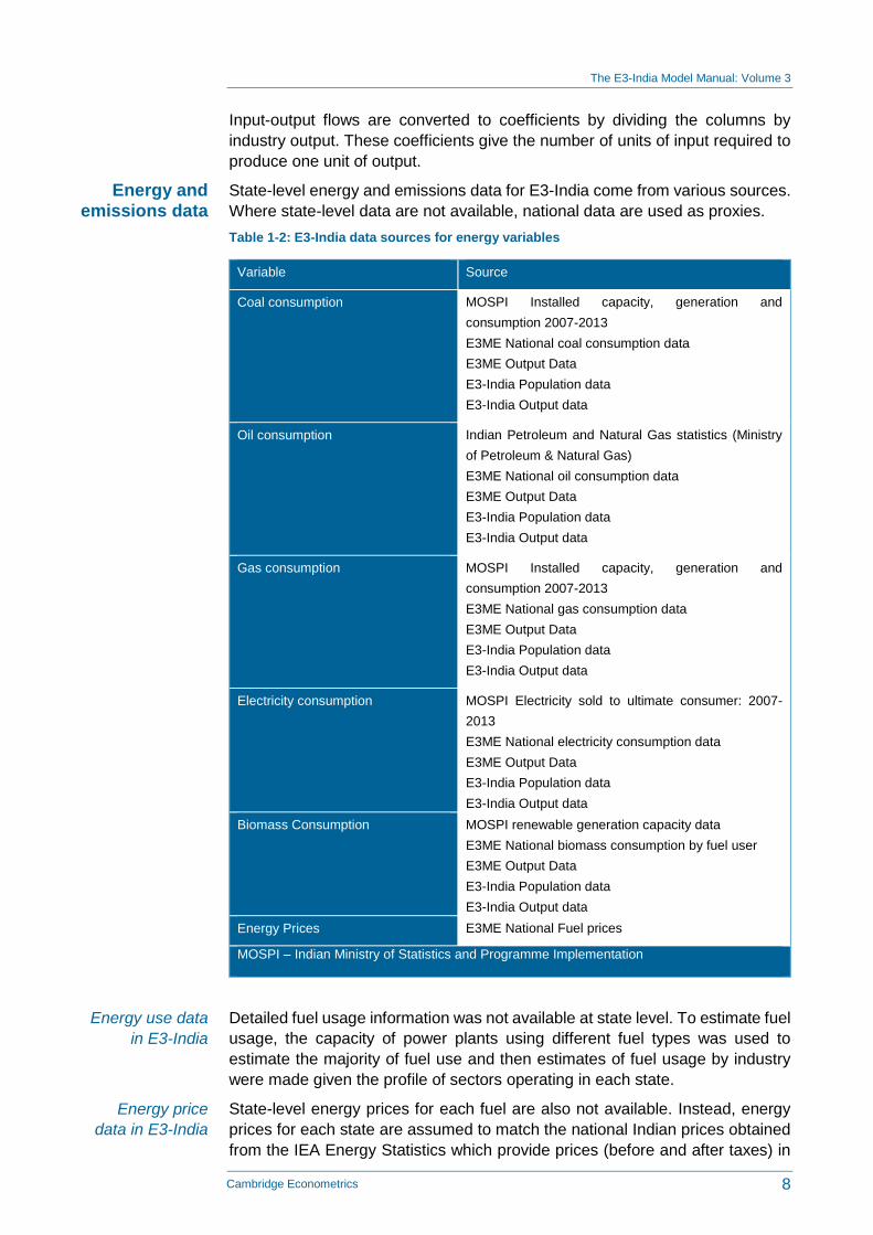
State-level energy and emissions data for E3-India come from various sources.

Where state-level data are not available, national data are used as proxies.

Table 1-2: E3-India data sources for energy variables

Variable Source

Coal consumption MOSPI Installed capacity, generation and

consumption 2007-2013

E3ME National coal consumption data

E3ME Output Data

E3-India Population data

E3-India Output data

Oil consumption Indian Petroleum and Natural Gas statistics (Ministry

of Petroleum & Natural Gas)

E3ME National oil consumption data

E3ME Output Data



Gas consumption MOSPI Installed capacity, generation and

consumption 2007-2013

E3ME National gas consumption data

E3ME Output Data



Electricity consumption MOSPI Electricity sold to ultimate consumer: 2007-

2013

E3ME National electricity consumption data

E3ME Output Data



Biomass Consumption MOSPI renewable generation capacity data

E3ME National biomass consumption by fuel user

E3ME Output Data



Energy Prices E3ME National Fuel prices

MOSPI – Indian Ministry of Statistics and Programme Implementation

Detailed fuel usage information was not available at state level. To estimate fuel

usage, the capacity of power plants using different fuel types was used to

estimate the majority of fuel use and then estimates of fuel usage by industry

were made given the profile of sectors operating in each state.

State-level energy prices for each fuel are also not available. Instead, energy

prices for each state are assumed to match the national Indian prices obtained

from the IEA Energy Statistics which provide prices (before and after taxes) in

Energy and emissions data

Energy use data

in E3-India

Energy price

data in E3-India



USD per tonne of oil equivalent by country and by fuel. Global fossil fuel price

data for oil, coal and gas also come from the IEA.

Time-series data for CO2 emissions, disaggregated by energy user, are

calculated using national emission coefficients.

The team at Cambridge Econometrics has developed a software package to fill

in gaps in any of the E3-India time series. The approach uses growth rates and

shares between sectors and variables to estimate missing data points, both in

cases of interpolation and extrapolation. Some time series have specific rules

for filling gaps in the data, but the general procedures are described here.

The most straightforward case is when the growth rates of a variable are known

and so the level can be estimated from these growth rates, as long as the initial

level is known. Sharing is used when the time-series data of an aggregation of

sectors are available but the individual time series is not. In this case, the

sectoral time series can be calculated by sharing the total, using either actual

or estimated shares.

In the case of extrapolation, it is often the case that aggregate data are available

but sectoral data are not; for example, government expenditure is a good proxy

for the total growth in education, health and defence spending. A special

procedure has been put in place to estimate the growth in more disaggregated

sectors so that the sum of these matches the known total, while the individual

sectoral growth follows the characteristics of each sector. Interpolation is used

when no external source is available, to estimate the path of change during an

interval, at the beginning and end of which data are available.

Under different assumptions, time-series forecasts are created for each country

and each aggregated variable: consumption, employment, GDP, trade and

investment (see Section 4).

E3-India’s software limits model variables to four character names. These

characters are typically used to identify first the dimensions of the variable

(excluding time, which is a dimension for all the variables) and then the indicator.

In particular, Q indicates disaggregation by product, Y by industry, F by energy

(fuel) user and R by region. If a variable name starts with P then it usually

indicates a price. S and 0 can be used to identify sums.

These conventions are used in the data processing and in the model itself.

Some examples of common variables names are provided below:

• QR: (Gross) output by product and by region

• YR: (Gross) output by industry and region

• YRE: Employment by industry and region

• YRW: Wage rates by industry and region

• YRVA: Gross value added by industry and region

• CR: Consumption by consumption category and region

• PCR: Consumption prices by category and region

• RSC: Total consumption by region

• PRSC: Aggregate consumer price by region

CO2 emissions in

E3-India

Correcting for missing data

points

Naming conventions



• KR: Investment by investment category and region

• FR0: Total energy consumption by energy user and region

• FRET: Electricity consumption by energy user and region

• FCO2: CO2 emissions by energy user and region

• RCO2: CO2 emissions by region

1.3 Econometric parameters

The econometric techniques used to specify the functional form of the equations

are the concepts of cointegration and error-correction methodology, particularly

as promoted by Engle and Granger (1987) and Hendry et al (1984).

In brief, the process involves two stages. The first stage is a levels relationship,

whereby an attempt is made to identify the existence of a cointegrating

relationship between the chosen variables, selected on the basis of economic

theory and a priori reasoning, e.g. for employment demand the list of variables

contains real output, real wage costs, hours-worked, energy prices and the two

measures of technological progress.

If a cointegrating relationship exists then the second stage regression is known

as the error-correction representation, and involves a dynamic, first-difference,

regression of all the variables from the first stage, along with lags of the

dependent variable, lagged differences of the exogenous variables, and the

error-correction term (the lagged residual from the first stage regression). Due

to limitations of data size, however, only one lag of each variable is included in

the second stage.

Stationarity tests on the residual from the levels equation are performed to

check whether a cointegrating set is obtained. Due to the size of the model, the

equations are estimated individually rather than through a cointegrating VAR.

For both regressions, the estimation technique used is instrumental variables,

principally because of the simultaneous nature of many of the relationships, e.g.

wage, employment and price determination.

E3-India’s parameter estimation is carried out using a customised set of

software routines based in the Ox programming language (Doornik, 2007). The

main advantage of using this approach is that parameters for all sectors and

countries may be estimated using an automated approach.

The estimation produces a full set of standard econometric diagnostics,

including standard errors and tests for endogeneity.

A list of equation results can be made available on request and parameters are

stored on the X databank. For each equation, the following information is given:

• summary of results

• full list of parameter results

• full list of standard deviations

Software used

Estimation results



1.4 Baseline forecast

The E3-India model can be used for forming a set of projections but it is usually

used only for policy analysis. Policy analysis is carried out in the form of a

baseline with additional policy scenarios, with the differences in results between

the scenarios and the baseline being attributed to the policy being assessed.

This section describes how the baseline is formed.

Usually results from E3-India scenarios are presented as (percentage)

difference from base, so at first it may appear that the actual levels in the

baseline are not important. However, analysis has shown that the values used

in the baseline can be very important in determining the outcomes from the

analysis. For example:

• If a scenario has a fixed emission target (e.g. 20% below 2005 levels) then

the baseline determines the amount of work that must be done in the

scenario to meet the target.

• If a scenario adds a fixed amount on to energy prices, then baseline energy

prices determine the relative (percentage) impact of that increase.

It is therefore important to have a baseline that does not introduce bias into the

scenario results. A common requirement of E3-India analysis is that the

baseline is made to be consistent with official published forecasts. Since we do

not have access to state-level economic and energy projections, the E3-India

baseline is calibrated to national projections from the World Energy Outlook

(IEA, 2015). State-level projections have been set to match.

The first stage in matching the E3-India projections to a published forecast is to

process these figures into a suitable format. This means that the various

dimensions of the model must be matched, including:

• geographical coverage (i.e. each state and territory)

• annual time periods

• sectoral coverage (including fuels and fuel users)

• National Accounts entries

CE uses the Ox software for carrying out this process, and saves the results on

to the forecast databank, F.db1.

The next stage is to solve the model to match the results on the forecast

databank. This is referred to as the ‘calibrated forecast’. In this forecast, the

model solves its equations and compares differences in results to the figures

that are saved on the databank. The model results are replaced with the

databank values but, crucially, the differences are stored and saved to another

databank, S.db1. These are referred to as ‘residuals’ although the meaning is

slightly different to the definition used in econometric estimation.

The final stage is the ‘endogenous solution’ in which the model equations are

solved but the residuals are added on to these results. In theory, the final

outcome should be the same as for the calibrated forecast, although in practice

there are calibration errors so it is not an exact match.

The key difference, however, is that inputs to the endogenous baseline may be

changed in order to produce a different outcome (as opposed to the calibrated

forecast where the model would still match databank values). The final outcome

Overview

Role of the

baseline

Methodology for calibrating

Endogenous

baseline and

scenarios



is thus a baseline forecast that matches the published projections, but which

can also be used for comparison with scenarios.

Consider an example for the aggregate consumption equation. If in the first year

of forecast, E3-India predicts a value of 100bn rupees but the published forecast

suggests 101bn rupees then the calibrated forecast will estimate a residual of

1.01 (i.e. 101/100).

If we then test a scenario in which consumption increases by 2% in this year,

the model results will be 100bn rupees (endogenous baseline) and 102bn

rupees (scenario). These will be adjusted (multiplied) by the residual to become

101bn rupees and 103.02bn rupees.

When these results are presented as percentage difference from base, the

figure that is reported is still 2% (103.02/101), so the calibration does not affect

directly the conclusions from the model results.

In this example, there is no impact on the results relative to baseline from the

calibration exercise. This is typically true for any log-linear relationship within

the model structure, as the calibration factors are cancelled out when calculating

differences from base.

However, there are relationships in the model that are not log-linear, most

commonly simple linear factors. These include the construction of energy prices

but also identities for GDP and for (gross) output, and the calculation for

unemployment (as labour supply minus demand).

For example, if the calibration results in higher trade ratios in a certain country,

then the effects that trade impacts have on GDP will increase in the scenarios.

It is therefore important that the baseline provides a reasonable representation

of reality, otherwise it is possible to introduce bias into the results.

1.5 Other model data inputs

In the current version of the model there are two additional text files that are

used as inputs (asides from the instruction file, see Volume 2). These are the

assumptions file and the scenario file, both of which can be modified by the

model user.

The reason for having these inputs as text files rather than databank entries is

that it allows easy manipulation, including through the Manager software (see

Volume 2, Section 2.). No programming expertise is therefore required to make

the changes.

The assumptions file contains basic economic information that is necessary for

any model run. It consists mainly of exogenous model variables that are set by

the model user.

The nature of the Fortran read commands means that the structure of the

assumptions text files is very rigid, for example with the right number of white

spaces (not tabs) and decimal places required for each entry.

The assumptions files cover the period 2000 to 2050 although historical values

will get overwritten by the data stored on the model databanks and the last year

of the model is 2035.

Operational example

When are results

influenced by

calibration?

Assumptions file



At the top of the assumption file is a set of global commodity prices, with a focus

on the energy groups that are covered by the model classifications. The figures

are annual growth rates, in percentage terms.

Also at the top of the assumption file there is a set of twelve other countries’

GDP assumptions that form demand for Indian exports. The E3-India model

assumes that rates of growth in the rest of the world are exogenous, matching

the numbers in the assumptions file. The figures are annual growth rates, in

percentage terms.

This is followed by a set of assumptions that are specific to each state. They

are:

• Market exchange rate (not used)

• Long-run interest rate

• Short-run interest rate (only used for comparative purposes)

• Change in government final consumption, year on year

• % of government consumption spent on defence, education and health

• Standard VAT rate

• Aggregate rate of direct taxes

• Average indirect tax rates

• Ratio of benefits to wages (giving implicit rate)

• Employees’ social security rate

• Employers’ social security rate

The scenario file contains a set of policy inputs that relate to basic model

scenarios (see examples in Volume 2, Section 4). It can also be modified

through the model Manager. Most of the policies in the scenario files are absent

in the baseline. Policy inputs in the scenario file are categorised to three main

groups: CO2 emissions policies, energy policies and options to recycle the

revenue generated from market-based instruments.

The following CO2 emissions policies are available in the scenarios file:

• annual CO2 tax rate, rupees per tonne of carbon

• switches to include different energy users in the policies

• switches to include different fuel types in the policies

The following energy policies are available in the scenario file:

• annual energy tax rate, rupees per toe

• switches to include different users in policies

• switch to include different fuel types in policies

• households implied price of electricity subsidies (see Volume 5, Section 3)

The scenario file includes options to recycle automatically the revenues

generated from carbon taxes and energy taxes (so that government balances

Commodity

prices

Other world

economies

National and

regional

assumptions

Scenarios file

CO2 emissions

policies

Energy policies

Revenue

recycling options



remain unchanged). There are three options in the scenario file for how the

revenues are recycled:

• to lower employers’ social security contributions, switch 0<X<1: 1=all, 0=

none

• to lower income tax rates, switch 0<X<1: 1=all, 0=none

• to lower VAT rates, switch 0<X<1: 1=all, 0= none

These revenue recycling options do not differentiate sources of revenues. The

model automatically sets the revenues to be recycled from the policies so that

they are overall ‘revenue neutral’. Specific values for offsetting tax reductions

can be entered through the assumption file discussed above.

1.6 Model outputs

The model produces relatively few results automatically. It instead stores results

internally so that they can be accessed separately. The separation of model

solution, (1) writing the results year by year to a large file (the ‘dump’), and then

(2) accessing this file to generate time series of results, is necessary because

of software constraints and the logic of the model.

Because of the scale of the solution, the model does not hold all the time series

of each variable, but only the current and past values necessary for the current

year's solution; this reduces the storage requirements dramatically (one year

plus lags instead of up to 50 years of values). At the completion of each year's

solution, the solved values of most variables are written to the dump where they

may be later accessed.

The files that access the model results are called data analysis files. They are

instruction files that are run after the model has finished solving (see Volume 2).

The file produced contains matrix output. These files are designed as inputs to

further processing, for example by other programming languages, or

interpretation by the model manager software (see Volume 2, Section 2). They

appear in the output directory with a ‘.MRE’ extension.

The data analysis files must start with a RESTART command with a year that

matches the PUT ALL statement in the IDIOM instruction file (usually the first

year of solution). A SELECT command then determines the output stream and

format:

• SELECT OUTPUT 7 CARDS – MRE output

The syntax is then relatively straight forward. The VALUE command is followed

by the variable name, start year and end year to give a table in time series

format. The CHANGE command gives the equivalent output as annual growth

rates. For variables with two dimensions (excluding time) it is necessary to say

which column is required. So, for example, the command:

• VALUE CR(?:03) 2013 2020

would give a time series for household consumption in Assam (region 3)

between 2013 and 2020. The following command will print out results for all

states:

Overview

Data analysis files



• VALA CR(?:01) 2013 2020

The other model outputs are created for diagnostic purposes. A small text file

(diagnostics.mre) is created automatically, which contains summary information

about whether the model has solved and, if not, which equation caused the

breakdown in solution. A longer ‘verification’ text file contains automatically

generated outputs from the model, including warnings and possible non-

convergences in the solution (see Volume 2, Section 4), which can be returned

to Cambridge Econometrics to assist with problems in solution. The verification

files are by convention given names that start with the letter Q and are stored in

the verification folder in the output directory.

Other model outputs



2 Model Validation

2.1 Introduction

Validation is an important part of the model-building process and especially so

for a tool as large and complex as E3-India. There are several steps to the

validation process:

• reviewing model data and the gaps in the data that have been filled out

• assessing the results of the econometric estimation

• validating the model as a system against the historical data

• running test scenarios and comparing results with expectations

Each of these steps is described in the following sections.

2.2 Reviewing model data

Compiling the E3-India database was an extensive exercise that included

many checking phases along the way. Standard checks were carried out on

the time series, for example to identify breaks in the series.

The review of the data focused more on how the different series fit together,

which is less easy to identify from simple plots of the data. Examples include

cases where output appears to be different from the sum of its component

parts. While the data would not be expected to match up exactly, large

discrepancies could be the source of bias in the results.

The model itself provides a useful framework with which to carry out these

tests, as it reports some of the key differences. Where large discrepancies

were found, the team went back to assess the original data. For example, one

instance of two states being entered in the wrong order was found.

The data in the E3-India database are also fully available to anyone who uses

the model. Individuals with expertise on particular sectors or states are

therefore able to further assess the data, and send any queries to the team.

This part of the validation is especially important where gaps in the data have

been estimated, as the software algorithms that are used may not always take

into account local context.

2.3 Assessing the results of the econometric estimation

Our estimation system is using the AIC to select the most appropriate set of

significant parameters in each equation. The explanatory factors in each

equation are selected based on the specification in the E3ME model. Outputs

from the estimation include the usual R-squared tests and tests of

significance. The more difficult bit to the evaluation is aggregating the tests

over equations that are estimated for each state and sector, i.e. managing the

amount of information that comes out of the estimation process.

The data as part of a system

External reviewing



We face two issues in the estimation – a lack of degrees of freedom, and a

data set that covers a period of transition and change in India. The estimation

results reflect both of these factors, although we anticipate that over time the

time series for estimation will be extended to improve the basis for the

estimation.

Three types of restrictions are placed on the coefficients that are estimated:

• Theoretical constraints – In a few cases restrictions are added to the

equations for theoretical reasons, e.g. to ensure a one-to-one relationship.

• ‘Right sign’ – For example, price elasticities are not allowed to be positive.

• Model stability – Maximum values are set to ensure the model remains

operable.

If the econometric estimation yields results that are overly constrained by

these restrictions then it could be an indication of issues in the data.

Figure 2.1 shows an example of a set of estimation results, from the equations

for employment (long-run part only, wages shown on an inverted scale). The

chart shows that 525 equations were estimated (x axis); that is all

sectors/states where there is employment. In around 50 cases no significant

relationship between wage rates and employment was found, and in around

100 cases no significant relationship between output and employment was

found.

At the other end of the scale, around 25 cases were found where the

relationship between output and employment was greater than one (i.e. a 1%

increase in output leads to more than a 1% increase in employment). For

wages, slightly more instances were found.

However, for the large majority of equations estimated, a relationship between

zero and one was found in both cases, giving impacts both in line with

expectations and stable enough to use in modelling.

Restrictions on the estimated

parameters

0.0

0.5

1.0

1.5

2.0

1 101 201 301 401 501

Co

effi

cien

t

Output Wages

Figure 2.1: Example estimation results (long-run employment equation)



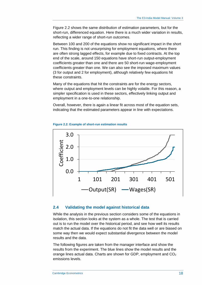
Figure 2.2 shows the same distribution of estimation parameters, but for the

short-run, differenced equation. Here there is a much wider variation in results,

reflecting a wider range of short-run outcomes.

Between 100 and 200 of the equations show no significant impact in the short

run. This finding is not unsurprising for employment equations, where there

are often strong lagged effects, for example due to fixed contracts. At the top

end of the scale, around 150 equations have short-run output-employment

coefficients greater than one and there are 50 short-run wage-employment

coefficients greater than one. We can also see the imposed maximum values

(3 for output and 2 for employment), although relatively few equations hit

these constraints.

Many of the equations that hit the constraints are for the energy sectors,

where output and employment levels can be highly volatile. For this reason, a

simpler specification is used in these sectors, effectively linking output and

employment in a one-to-one relationship.

Overall, however, there is again a linear fit across most of the equation sets,

indicating that the estimated parameters appear in line with expectations.

Figure 2.2: Example of short-run estimation results

2.4 Validating the model against historical data

While the analysis in the previous section considers some of the equations in

isolation, this section looks at the system as a whole. The test that is carried

out is to run the model over the historical period, and see how well its results

match the actual data. If the equations do not fit the data well or are biased on

some way then we would expect substantial divergence between the model

results and the data.

The following figures are taken from the manager interface and show the

results from the experiment. The blue lines show the model results and the

orange lines actual data. Charts are shown for GDP, employment and CO2

emissions levels.

0.0

1.0

2.0

3.0

1 101 201 301 401 501

Co

effi

cien

t

Output(SR) Wages(SR)



Figure 2.3: Historical validation, national level



Solving the model over the historical period is a considerable exercise, as in

general the model is designed to reproduce historical data rather than solve

the equations. In some cases the discrepancies reported may reflect

limitations in how the model solves historically rather than issues with model

equations but this section reports results as they are.

Overall, the model matches GDP closely but the chart shows a bigger

discrepancy for employment, led by differences in 1997-1999. The overall

difference amounts to about 10%. For CO2, the model results are also

consistently higher and again the difference is around 10%.

One important point to note for CO2, however, is that the power sector is not

included in the historical analysis, as the FTT model cannot be run over

history. FTT has its own structural validation, which is described in Mercure

(2012).

In general, however, results are encouraging in that they show some

differences (as expected) but no persistent bias. It is clear that there are some

developments just before 2000 that the model has not accounted for as well

as changes in other time periods but the general directions of the relationships

are consistent.

Figure 2.4 shows the pattern across states in terms of absolute difference

between model result and actual data. A few states stand out, which can

usually be traced to individual equations but the results are generally

consistent with those found at national level.

Figure 2.4: Historical validation - GDP at state level



2.5 Validating the model with residual corrections

The final test compares model results against actual data if we account for the

errors in the individual equations. The errors, which are referred to as

residuals, in the model interface are stored and added back into the

endogenous model solution; this is the same mechanism that is used by the

model to match baseline forecasts.

If the errors from the equations are large, then this approach could introduce

bias into the modelling, but this would have been picked up in the tests in the

previous section. This final test is more an assessment of the model’s

mechanics; we would expect it to very closely match the actual data. However,

the test is also important, because this is the closest approximation to how the

model is used for analysis.

Figure 2.5 confirms that this is the case, with no difference at all in the GDP

(and employment) results and only a very small difference in emissions.

Figure 2.5: Historical validation, including residual correction



Similar results were found at state level, with the discrepancies between

model results and actual data being only a fraction of a percent. These small

differences are likely due to rounding errors in the model solution process and

not an indication of issues in the underlying data and equations.

2.6 Running test scenarios

The final stage of the testing is for the model to be used as widely as possible

by individuals with a range of expertise to consider a range of different

policies. This part of the validation is still ongoing and we anticipate that some

of the exercises will be added as case studies to Volume 8 of this manual. Any

issues that are uncovered in this process will be investigated by the modelling

team.

2.7 Summary

In conclusion, extensive testing has been carried out as part of the model

validation and is still ongoing through an interactive process. Several issues,

relating to both data and features of the model code, have been identified

along the way and have been addressed.

The results presented in this chapter summarise the main findings of the

validation. While there is still work to be done in some of the individual

equations, we expect this to move forward over time as additional data

become available. Longer time series should improve the accuracy of the

parameter estimation and may allow for additional explanatory variables to be

added to the equations, without reducing degrees of freedom too much.

The focus now is on developing additional test scenarios to continuously

further model validation.



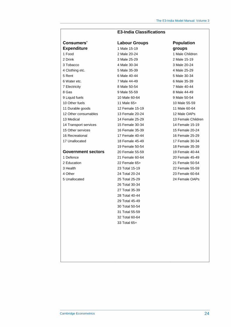
Appendix A Model Classifications

Regions

1 Andhra Pradesh

2 Arunachal Pradesh

3 Assam

4 Bihar

5 Chhattisgarh

6 Gujarat

7 Haryana

8 Himachal Pradesh

9 Goa

10 Jammu & Kashmir

11 Jharkhand

12 Karnataka

13 Kerala

14 Madhya Pradesh

15 Maharashtra

16 Manipur

17 Meghalaya

18 Mizoram

19 Nagaland

20 Orissa

21 Punjab

22 Rajasthan

23 Sikkim

24 Tamil Nadu

25 Tripura

26 Uttar Pradesh

27 Uttarakhand

28 West Bengal

29 Andaman & Nicobar

30 Chandigarh

31 Delhi

32 Puducherry

E3-India Classifications

Sectors

1 Agriculture

2 Forestry & Logging

3 Fishing

4 Coal Extraction

5 Oil Extraction

6 Gas Extraction

7 Non-Energy Mining

8 Manufacturing

9 Electricity

10 Gas

11 Water

12 Construction

13 Transport & Storage

14 Communication

15 Trade, Hotels & Restaurants

16 Banking & Insurance

17 Real Estate

18 Other Business Services

19 Public Administration

20 Other Services

Fuel Users

1 Power generation

2 Other transformation

3 Manufacturing

4 Transport

5 Households

6 Services

7 Agriculture

8 Non-energy used

Fuels

1 Coal

2 Oil

3 Natural Gas

4 Electricity

5 Biomass



Consumers’

Expenditure

1 Food

2 Drink

3 Tobacco

4 Clothing etc.

5 Rent

6 Water etc.

7 Electricity

8 Gas

9 Liquid fuels

10 Other fuels

11 Durable goods

12 Other consumables

13 Medical

14 Transport services

15 Other services

16 Recreational

17 Unallocated

Government sectors

1 Defence

2 Education

3 Health

4 Other

5 Unallocated

E3-India Classifications

Labour Groups

1 Male 15-19

2 Male 20-24

3 Male 25-29

4 Male 30-34

5 Male 35-39

6 Male 40-44

7 Male 44-49

8 Male 50-54

9 Male 55-59

10 Male 60-64

11 Male 65+

12 Female 15-19

13 Female 20-24

14 Female 25-29

15 Female 30-34

16 Female 35-39

17 Female 40-44

18 Female 45-49

19 Female 50-54

20 Female 55-59

21 Female 60-64

22 Female 65+

23 Total 15-19

24 Total 20-24

25 Total 25-29

26 Total 30-34

27 Total 35-39

28 Total 40-44

29 Total 45-49

30 Total 50-54

31 Total 55-59

32 Total 60-64

33 Total 65+

Population

groups

1 Male Children

2 Male 15-19

3 Male 20-24

4 Male 25-29

5 Male 30-34

6 Male 35-39

7 Male 40-44

8 Male 44-49

9 Male 50-54

10 Male 55-59

11 Male 60-64

12 Male OAPs

13 Female Children

14 Female 15-19

15 Female 20-24

16 Female 25-29

17 Female 30-34

18 Female 35-39

19 Female 40-44

20 Female 45-49

21 Female 50-54

22 Female 55-59

23 Female 60-64

24 Female OAPs



Appendix B Model Inputs and Outputs

B.1 Model inputs

In the assumptions file there are two types of inputs, commodity prices and

GDP in other parts of the world. Both are expressed as annual growth rates.

The categories are:

• 02 CPRICE_FOOD_FEED – prices for food and animal feed

• 03 CPRICE_WOOD – prices for wood as a raw material

• 04 CPRICE_CONS_MIN – prices for aggregates and other construction

minerals

• 05 CPRICE_IND_MIN – prices for minerals used for industrial purposes

• 06 CPRICE_FER_ORES – prices for ferrous ores

• 07 CPRICE_NFER_ORES – prices for non-ferrous ores

• 08 CPRICE_COAL – coal prices

• 09 CPRICE_BRENT_OIL – oil prices

• 10 CPRICE_GAS – natural gas prices

• 11 CPRICE_OTHERS – prices for other commodities

The countries for which GDP growth can be adjusted are India’s main trading

partners. Other countries are included in the final rest of world category.

The inputs in the scenarios file are:

Input Units Dimensions Definition

RTEA Rup/toe State x Year Energy tax levied on energy

consumption

RTCA Rup/tC State x Year Carbon tax levied on CO2

emissions

FEDS Share Fuel User x

State

Exemptions from RTCA and

RTEA, 0 = exempt

JEDS Share Fuel x State Exemptions from RTCA and

RTEA, 0 = exempt

RRTE % State x Year Carbon/energy tax revenues

used to reduce employers’

social contributions

RRTR % State x Year Carbon/energy tax revenues

used to reduce income taxes

RRVT % State x Year Carbon/energy tax revenues

used to reduce VAT

PESH Share Income Group

x State

Implied subsidies to each

group (1 = none)

Assumptions file

Scenarios file



Additional flexibility is added when using the instructions files. Some of the

most commonly used inputs here are shown below.

• FRCH (fuel user by state) – exogenous reduction in coal consumption, in

thousands of tonnes of oil equivalent.

• FROH, FRGH, FREH – exogenous reductions in oil, gas and electricity

consumptions (same dimensions and units).

• KRX (sector by state) – exogenous increase in investment, millions of

rupees at 2010 prices.

Almost all the variables in E3-India can be shocked exogenously. For further

information on this please contact the modelling team.

Other inputs (through the instructions

files)



B.2 Model outputs

The interface provides a long list of potential outputs (and more can be

added). The key ones are listed here.

Output Units Dimensions Definition

RGDP mR (2010) State GDP at market prices

RSC mR (2010) State Household consumption

RSK mR (2010) State Investment (GFCF)

RSX mR (2010) State Export volumes

RSM mR (2010) State Import volumes

PRSC 2010=1.0 State Consumer price index

RRPD mR (2010) State Real household incomes

CR mR (2010) Product x state Disaggregated consumption

KR mR (2010) Sector x state Investment

QRX mR (2010) Sector x state Exports

QRM mR (2010) Sector x state Imports

PYH 2010=1.0 Sector x state Domestic production prices

PQRD 2010=1.0 Sector x state Domestic consumption prices


YRE thousands Sector x state Employment

YRW thR/year Sector x state Wage rates (current price)

RWPP thousands State Labour supply

RUNE thousands State Unemployment

RUNR % State Unemployment rate

Economic outputs

Labour market outputs




FR0 th toe Fuel user x state Energy consumption

FRCT th toe Fuel user x state Coal consumption

FROT th toe Fuel user x state Oil consumption

FRGT th toe Fuel user x state Gas consumption

FRET th toe Fuel user x state Electricity consumption

PFR0 R / toe Fuel user x state Aggregate energy price

PFRC R / toe Fuel user x state Coal prices

PFRO R / toe Fuel user x state Oil prices

PFRG R / toe Fuel user x state Gas prices

PFRE R / toe Fuel user x state Electricity prices

MEWG GWh Technology x state Electricity generation

MEWK GWh Technology x state Electricity capacity


RCO2 th tC State CO2 emissions

FCO2 th tC Fuel user x state CO2 emissions

RCTT mR State Carbon tax revenues

Energy system outputs

Emissions outputs

The E3-India Model Manual: Volume 3 - Cambridge …€¦ · · 2017-08-11series covering the...

Documents

Transcript of The E3-India Model Manual: Volume 3 - Cambridge …€¦ · · 2017-08-11series covering the...